Evaluation of Page

Replacement Algorithms in a Geographic

Information System

D A N I E L H U L T G R E N

Master of Science Thesis Stockholm, Sweden 2012

Evaluation of Page

Replacement Algorithms in a Geographic

Information System

D A N I E L H U L T G R E N

DD221X, Master’s Thesis in Computer Science (30 ECTS credits) Degree Progr. in Computer Science and Engineering 300 credits Master Programme in Computer Science 120 credits Royal Institute of Technology year 2012 Supervisor at CSC was Alexander Baltatzis Examiner was Anders Lansner TRITA-CSC-E 2012:073 ISRN-KTH/CSC/E--12/073--SE ISSN-1653-5715 Royal Institute of Technology School of Computer Science and Communication KTH CSC SE-100 44 Stockholm, Sweden URL: www.kth.se/csc

AbstractCaching can improve computing performance significantly. In this paperI look at various page replacement algorithms in order to make a cachein two levels – one in memory and one on a hard drive. Both levelspresent unique limitations and possibilities: the memory is limited insize but very fast while the hard drive is slow and so large that memoryindexing often is not feasible.

I also propose several hard drive based algorithms with varying lev-els of memory consumption and performance, allowing for a trade-offto be made. Further, I propose a variation for existing memory algo-rithms based on the characteristics of my test data. Finally, I choosethe algorithms I consider best for my specific case.

ReferatUtvärdering av cachningsalgoritmer i ett geografiskt

informationsystem

Cachning av data kan förbättra datorers prestanda markant. I den härrapporten undersöker jag ett antal cachningsalgoritmer i syfte att skapaen cache i två nivåer – en minnescache och en diskcache. Båda nivåernahar unika begränsningar och möjligheter: minnet är litet men väldigtsnabbt medan hårddisken är långsam och så stor att minnesindexeringofta inte är rimligt.

Jag utvecklar flera hårddiskbaserade algoritmer med varierande gradav minneskonsumption och prestanda, vilket innebär att man kan väljaalgoritm baserat på klientens förutsättningar. Vidare föreslår jag en va-riation till existerande algoritmer baserat på min testdatas egenskaper.Slutligen väljer jag de algoritmer jag anser bäst för mitt specifika fall.

Contents

1 Introduction 11.1 Problem statement . . . . . . . . . . . . . . . . . . . . . . . . . . . . 11.2 Goal . . . . . . . . . . . . . . . . . . . . . . . . . . . . . . . . . . . . 11.3 About Carmenta . . . . . . . . . . . . . . . . . . . . . . . . . . . . . 2

2 Background 32.1 What is a cache? . . . . . . . . . . . . . . . . . . . . . . . . . . . . . 32.2 Previous work . . . . . . . . . . . . . . . . . . . . . . . . . . . . . . . 3

2.2.1 In page replacement algorithms . . . . . . . . . . . . . . . . . 42.2.2 Why does LRU work so well? . . . . . . . . . . . . . . . . . . 52.2.3 In map caching . . . . . . . . . . . . . . . . . . . . . . . . . . 6

2.3 Multithreading . . . . . . . . . . . . . . . . . . . . . . . . . . . . . . 62.3.1 Memory . . . . . . . . . . . . . . . . . . . . . . . . . . . . . . 62.3.2 Hard drive . . . . . . . . . . . . . . . . . . . . . . . . . . . . 72.3.3 Where is the bottleneck? . . . . . . . . . . . . . . . . . . . . 7

2.4 OGC – Open Geospatial Consortium . . . . . . . . . . . . . . . . . . 8

3 Testing methodology 93.1 Aspects to test . . . . . . . . . . . . . . . . . . . . . . . . . . . . . . 9

3.1.1 Hit rate . . . . . . . . . . . . . . . . . . . . . . . . . . . . . . 93.1.2 Speed . . . . . . . . . . . . . . . . . . . . . . . . . . . . . . . 93.1.3 Hit rate over time . . . . . . . . . . . . . . . . . . . . . . . . 10

3.2 The chosen algorithms . . . . . . . . . . . . . . . . . . . . . . . . . . 103.2.1 First In, First Out (FIFO) . . . . . . . . . . . . . . . . . . . . 103.2.2 Least Recently Used (LRU) . . . . . . . . . . . . . . . . . . . 103.2.3 Least Frequently Used (LFU) and modifications . . . . . . . 103.2.4 Two Queue (2Q) . . . . . . . . . . . . . . . . . . . . . . . . . 113.2.5 Multi Queue (MQ) . . . . . . . . . . . . . . . . . . . . . . . . 113.2.6 Adaptive Replacement Cache (ARC) . . . . . . . . . . . . . . 113.2.7 Algorithm modifications . . . . . . . . . . . . . . . . . . . . . 11

3.3 Proposed algorithms . . . . . . . . . . . . . . . . . . . . . . . . . . . 113.3.1 HDD-Random . . . . . . . . . . . . . . . . . . . . . . . . . . 123.3.2 HDD-Random Size . . . . . . . . . . . . . . . . . . . . . . . . 12

3.3.3 HDD-Random Not Recently Used (NRU) . . . . . . . . . . . 123.3.4 HDD-Clock . . . . . . . . . . . . . . . . . . . . . . . . . . . . 133.3.5 HDD-True Random . . . . . . . . . . . . . . . . . . . . . . . 133.3.6 HDD-LRU with batch removal . . . . . . . . . . . . . . . . . 143.3.7 HDD-backed memory algorithm . . . . . . . . . . . . . . . . 14

4 Analysis of test data 174.1 Data sources . . . . . . . . . . . . . . . . . . . . . . . . . . . . . . . 174.2 Pattern analysis . . . . . . . . . . . . . . . . . . . . . . . . . . . . . . 174.3 Locality analysis . . . . . . . . . . . . . . . . . . . . . . . . . . . . . 184.4 Access distribution . . . . . . . . . . . . . . . . . . . . . . . . . . . . 194.5 Size distribution . . . . . . . . . . . . . . . . . . . . . . . . . . . . . 20

5 Results 235.1 Memory cache . . . . . . . . . . . . . . . . . . . . . . . . . . . . . . . 23

5.1.1 The size modification . . . . . . . . . . . . . . . . . . . . . . 245.1.2 Pre-population . . . . . . . . . . . . . . . . . . . . . . . . . . 245.1.3 Speed . . . . . . . . . . . . . . . . . . . . . . . . . . . . . . . 27

5.2 Hard drive cache . . . . . . . . . . . . . . . . . . . . . . . . . . . . . 275.3 Conclusion . . . . . . . . . . . . . . . . . . . . . . . . . . . . . . . . 285.4 Future work . . . . . . . . . . . . . . . . . . . . . . . . . . . . . . . . 29

Bibliography 31

Chapter 1

Introduction

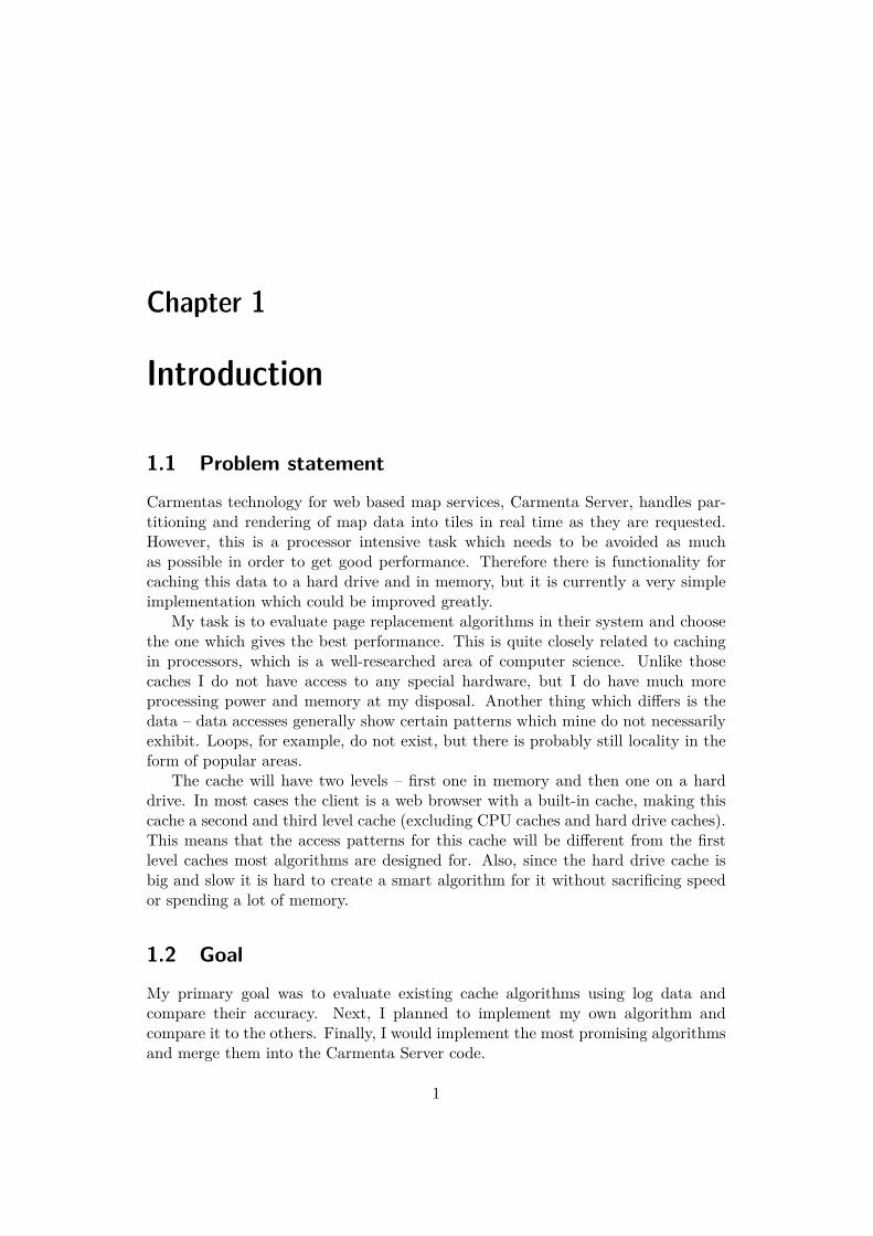
1.1 Problem statement

Carmentas technology for web based map services, Carmenta Server, handles par-titioning and rendering of map data into tiles in real time as they are requested.However, this is a processor intensive task which needs to be avoided as muchas possible in order to get good performance. Therefore there is functionality forcaching this data to a hard drive and in memory, but it is currently a very simpleimplementation which could be improved greatly.

My task is to evaluate page replacement algorithms in their system and choosethe one which gives the best performance. This is quite closely related to cachingin processors, which is a well-researched area of computer science. Unlike thosecaches I do not have access to any special hardware, but I do have much moreprocessing power and memory at my disposal. Another thing which differs is thedata – data accesses generally show certain patterns which mine do not necessarilyexhibit. Loops, for example, do not exist, but there is probably still locality in theform of popular areas.

The cache will have two levels – first one in memory and then one on a harddrive. In most cases the client is a web browser with a built-in cache, making thiscache a second and third level cache (excluding CPU caches and hard drive caches).This means that the access patterns for this cache will be different from the firstlevel caches most algorithms are designed for. Also, since the hard drive cache isbig and slow it is hard to create a smart algorithm for it without sacrificing speedor spending a lot of memory.

1.2 Goal

My primary goal was to evaluate existing cache algorithms using log data andcompare their accuracy. Next, I planned to implement my own algorithm andcompare it to the others. Finally, I would implement the most promising algorithmsand merge them into the Carmenta Server code.

1

CHAPTER 1. INTRODUCTION

1.3 About CarmentaCarmenta is a software/consulting company working with geographic informationsystems (GIS). The company was founded in 1985 and has about 60 employees.They have two main products: Carmenta Engine and Carmenta Server. CarmentaEngine is the system core which focuses on visualizing and processing complexgeographical data. It has functionality for efficiently simulating things such as lineof sight and thousands of moving objects.

Carmenta Server is an abstraction layer used to simplify distribution of mapsover intranets and the internet. It is compliant with several open formats makingit easy to create custom-made client applications, and there are also several opensource applications which can be used directly.

Carmentas technology is typically used by customers who require great controlover the way they present and interact with their GIS. For example, the Swedishmilitary uses Carmenta Engine for their tactical maps and SOS Alarm uses it tooverlay their maps with various information and images useful for the rescue work-ers.

2

Chapter 2

Background

In this chapter I give a short presentation of what a cache is, why caching is impor-tant and some previous work in the area.

2.1 What is a cache?

In short, a cache is a component which transparently stores data in order to accesssaid data faster in the future. For example, if a program repeats a calculation severaltimes the result could be stored in a cache (cached) after the first calculation andthen retrieved from there the next time the program needs it. This has potential tospeed up program execution greatly. The exact numbers vary between systems, butseeking on a hard drive takes roughly 10ms and referencing data in the L1 cacheroughly 0.5ns. Thus, caching data from the hard drive in the L1 cache could intheory speed up the next request 2 × 107 times!

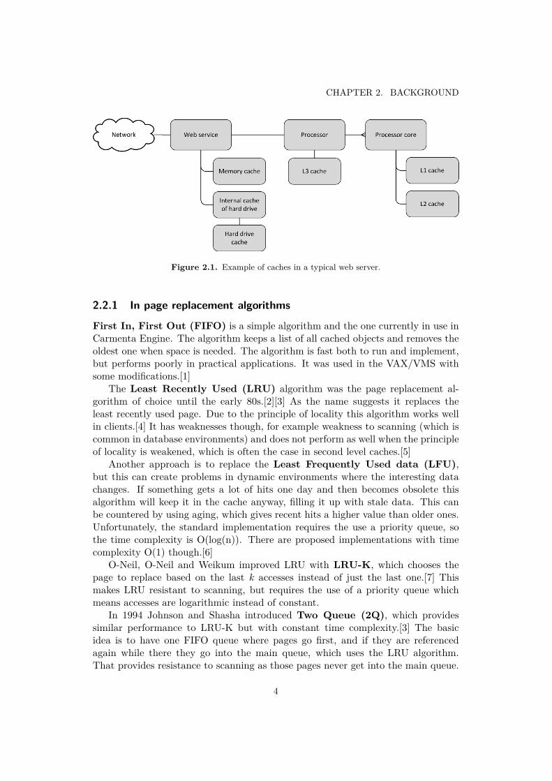
There are caches on many different levels in a computer. For example, modernprocessors contain three cache levels, named L1-L3. L1 is closest to the processorcore and L3 is shared among all cores. The closer they are to the core, the smallerand faster they are. Operating systems and programs typically cache data in mem-ory as well. While the processor caches are handled by hardware, this caching isdone in software and the cached data is chosen by the programmer. Also, harddrives typically have caches to avoid having to move the read heads when com-monly used data is requested. Finally, programs can use the hard drive to cachedata which would be very slow to get, for example data that would need substantialcalculations or network requests.

2.2 Previous work

Page replacement algorithms have long been an important area of computer science.I will mention a few algorithms which are relevant to this paper but there are manymore, and several variations of them.

3

CHAPTER 2. BACKGROUND

Figure 2.1. Example of caches in a typical web server.

2.2.1 In page replacement algorithms

First In, First Out (FIFO) is a simple algorithm and the one currently in use inCarmenta Engine. The algorithm keeps a list of all cached objects and removes theoldest one when space is needed. The algorithm is fast both to run and implement,but performs poorly in practical applications. It was used in the VAX/VMS withsome modifications.[1]

The Least Recently Used (LRU) algorithm was the page replacement al-gorithm of choice until the early 80s.[2][3] As the name suggests it replaces theleast recently used page. Due to the principle of locality this algorithm works wellin clients.[4] It has weaknesses though, for example weakness to scanning (which iscommon in database environments) and does not perform as well when the principleof locality is weakened, which is often the case in second level caches.[5]

Another approach is to replace the Least Frequently Used data (LFU),but this can create problems in dynamic environments where the interesting datachanges. If something gets a lot of hits one day and then becomes obsolete thisalgorithm will keep it in the cache anyway, filling it up with stale data. This canbe countered by using aging, which gives recent hits a higher value than older ones.Unfortunately, the standard implementation requires the use a priority queue, sothe time complexity is O(log(n)). There are proposed implementations with timecomplexity O(1) though.[6]

O-Neil, O-Neil and Weikum improved LRU with LRU-K, which chooses thepage to replace based on the last k accesses instead of just the last one.[7] Thismakes LRU resistant to scanning, but requires the use of a priority queue whichmeans accesses are logarithmic instead of constant.

In 1994 Johnson and Shasha introduced Two Queue (2Q), which providessimilar performance to LRU-K but with constant time complexity.[3] The basicidea is to have one FIFO queue where pages go first, and if they are referencedagain while there they go into the main queue, which uses the LRU algorithm.That provides resistance to scanning as those pages never get into the main queue.

4

2.2. PREVIOUS WORK

Megiddo and Modha introduced the Adaptive Replacement Cache (ARC)which bears some similarities to 2Q.[8] Just like 2Q it is composed of two mainqueues, but where 2Q requires that the user tunes the size of the different queuesmanually ARC uses so called ghost lists to dynamically adapt their sizes dependingon the workload. More details can be found in their paper. This allows ARC toadapt better than 2Q, which further improves hit rate. However, IBM has patentedthis algorithm, which might cause problems if it is used in commercial applications.Megiddo and Modha also adapted Clock with adaptive replacement[9], but theperformance is similar to ARC and it is also patented, so it will not be evaluated.

In a slightly different direction, Zhou and Philbin introduced Multi-Queue(MQ), which aims to improve cache hit rate in second level buffers.[5] The previousalgorithms mentioned in this paper were all aimed at first level caches, so this cachehas different requirements. Accesses to a second level cache are actually misses fromthe first level, so the access pattern is different. In their report they show that theprinciple of locality is weakened in their traces and that frequency is more importantthan recency. Their algorithm is based around multiple LRU queues. As pages arereferenced they get promoted to queues with other highly referenced pages. Whenpages need to be removed they are taken from the lesser referenced queues, andthere is also an aging mechanism to remove stale pages. This strengthens frequencybased choice while still having an aspect of recency. This proved to work well forsecond level caches and is interesting for my problem.

Another notable page replacement algorithm is Bélády’s algorithm, also knownas Bélády’s optimal page replacement policy.[10] It works by always removing thepage whose next use will occur farthest in the future. This will always yield optimalresults, but is generally not applicable in reality since it needs to know exactly whatwill be accessed and in which order. It is however used as an upper bound of howgood hit rate an algorithm can have.

We have a large number of page replacement algorithms, all with differentstrengths and weaknesses. It is hard to pinpoint the best one as that dependson how it will be used. Understanding access patterns is integral to designing orchoosing the best cache algorithm, and that will be dealt with later in this paper.

2.2.2 Why does LRU work so well?

As explained in Chapter 2.2.1 there are a lot of page replacement algorithms basedaround LRU. This is because of a phenomenon known as locality of reference. It iscomposed of several different kinds of locality, but the most important are spatialand temporal locality.[4] These laws state that if a memory location is referencedat a particular time it is likely that it or a nearby memory location will be refer-enced in the near future. This is because of how computer programs are written –they will often loop over arrays of data which are near each other in memory andaccess the same or nearby elements several times. With the rise of object orientedprogramming languages and more advanced data structures such as heaps, treesand hash tables locality of reference has been weakened somewhat, but it is still

5

CHAPTER 2. BACKGROUND

important to consider.[11]Locality of reference is further weakened for caches in server environments that

are not first level caches. This was explored by Zhou and Philbin and their MQalgorithm is the only one in the previous part that is made for server use.[5] Theyfound that the close locality of reference was very weak since they had already beentaken care of by previous caches. This depends heavily on the environment thecache is used in and does not necessarily apply to my situation.

2.2.3 In map caching

Generally, caches are placed in front of the application server. They take the re-quests from the clients and relay only the requests they cannot fulfill from the cache.Then they transparently save the data they get from the application server beforethey send it to the client. This makes the cache completely transparent to the ap-plication server, but means it needs to provide a full interface towards the client.Also, unless the server also provides the same interface it will not be possible toturn it off.

There are several free, open source alternatives that handle caching for WMS-compatible servers. Examples include GeoWebCache, TileCache and MapCache.They are all meant to be placed in front of the server and handle caching trans-parently. They aim at handling things like coordinating information from multiplesources (something made possible and smooth by WMS, which I will mention later)rather than being smooth so set up. They also often allow for several different cachemethods: MapCache can not only use a regular disk cache but also memcached,GoogleDisk, Amazon S3 and SQLite caches.[12] This makes them very flexible, butwhat Carmenta wants is a specific solution that is easy to set up.

Carmentas cache is optional, so it is currently a slave of Carmenta Server. Thissimplifies things, but since even cached requests have to go through the engine itreduces performance slightly. The cache works the same though, the only differenceis that requests come from the server instead of the client, and the server calls astore routine when the data is not in the cache.

2.3 MultithreadingMultithreading could potentially improve program throughput, and in this sectionI explore the possibilities of multithreading memory and hard drive accesses.

2.3.1 Memory

Modern memory architectures have a bus wide enough to allow for several memoryaccesses in parallel. This means that in order to get the full bandwidth from thememory several accesses need to run in parallel. Logically, this would mean thata multithreaded approach would run faster, but modern processors have alreadysolved that for us. Not only do they reorder operations on the fly but they also

6

2.3. MULTITHREADING

access memory in an asynchronous fashion, meaning that a single thread can runseveral accesses in parallel.

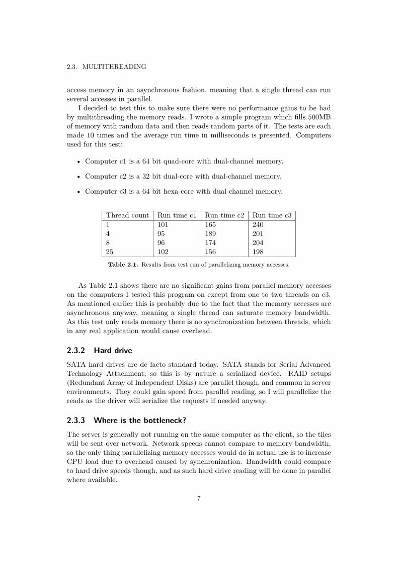
I decided to test this to make sure there were no performance gains to be hadby multithreading the memory reads. I wrote a simple program which fills 500MBof memory with random data and then reads random parts of it. The tests are eachmade 10 times and the average run time in milliseconds is presented. Computersused for this test:

• Computer c1 is a 64 bit quad-core with dual-channel memory.

• Computer c2 is a 32 bit dual-core with dual-channel memory.

• Computer c3 is a 64 bit hexa-core with dual-channel memory.

Thread count Run time c1 Run time c2 Run time c31 101 165 2404 95 189 2018 96 174 20425 102 156 198Table 2.1. Results from test run of parallelizing memory accesses.

As Table 2.1 shows there are no significant gains from parallel memory accesseson the computers I tested this program on except from one to two threads on c3.As mentioned earlier this is probably due to the fact that the memory accesses areasynchronous anyway, meaning a single thread can saturate memory bandwidth.As this test only reads memory there is no synchronization between threads, whichin any real application would cause overhead.

2.3.2 Hard driveSATA hard drives are de facto standard today. SATA stands for Serial AdvancedTechnology Attachment, so this is by nature a serialized device. RAID setups(Redundant Array of Independent Disks) are parallel though, and common in serverenvironments. They could gain speed from parallel reading, so I will parallelize thereads as the driver will serialize the requests if needed anyway.

2.3.3 Where is the bottleneck?The server is generally not running on the same computer as the client, so the tileswill be sent over network. Network speeds cannot compare to memory bandwidth,so the only thing parallelizing memory accesses would do in actual use is to increaseCPU load due to overhead caused by synchronization. Bandwidth could compareto hard drive speeds though, and as such hard drive reading will be done in parallelwhere available.

7

CHAPTER 2. BACKGROUND

When the cache misses the tile needs to be re-rendered. This should be avoidedas much as possible, as re-rendering can easily be slower than the network con-nection. As such, the key to good cache performance is getting a good hit rate.Multithreading is not needed for the memory part but is worth implementing ifthere are heavy calculations involved. However, reading from disk and from mem-ory should naturally be done in parallel.

2.4 OGC – Open Geospatial ConsortiumThe Open Geospatial Consortium is an international industry consortium that de-velops open interfaces for location-based services. Using an OGC standard meansthat the program becomes interoperable with several other programs on the mar-ket, making it more versatile. Carmenta is a member of OGC and Carmenta Serverimplements a standard called WMS, which ”specifies how individual map serversdescribe and provide their map content”.[13] The exact specification can be foundon their web page, but most of it is out of scope for this paper. In short, the clientcan request a rectangle of any size from any location of the map, with any zoomlevel, any format, any projection and a few other parameters.

The large amount of parameters create a massive amount of possible combina-tions which makes this data hard and inefficient to cache. To counter this an un-official standard has been developed: WMS-C.[14] In order to reduce the possiblecombinations the arguments are reduced, only one output format and projection isspecified, clients can only request fixed size rectangles from a given map grid amongother restrictions.

Carmenta uses WMS-C in their clients, and this is the usage I will be developingthe cache algorithm for.

8

Chapter 3

Testing methodology

In this chapter I discuss which aspects of the caches to test and present the algo-rithms I will test.

3.1 Aspects to testThere are two main aspects of a cache that are testable: speed and hit rate. Thesecould both be summarized into a single measurement: throughput. The problemwith that in my environment is that the time it takes to render a new tile differsgreatly depending on how the maps are configured. I decided to measure themseparately and weight them mostly based on hit rate. In the end their run timesended up very similar anyway, except for LFU.

3.1.1 Hit rate

The primary objective for this cache is to get a good hit rate. Hit rate is comparedat a specific cache size and a specific trace. In order to know where the cache foundits data I simply added a return parameter which told the test program where thedata was found.

3.1.2 Speed

Speed is harder to test than hit rate for several reasons:

• The hard drive has a cache.

• The operating system maintains its own cache in memory.

• The CPU has several caches.

• JIT compilation and optimization can cause inconsistent results.

• The testing hardware can work better with specific algorithms.

9

CHAPTER 3. TESTING METHODOLOGY

Focus for this cache is on hit rate, but I have run some speed tests as well. Whendoing speed tests I took several precautions to get as good results as possible:

• Hard drive cache and Carmenta Engine are not used for misses. Instead, Igenerate random data of correct size for the tiles.

• The tests are run several times before the timed run to make sure any JIT isdone before the actual run.

• I did not run any speed test on the hard drive caches.

Also, since the bottleneck is the memory rather than the CPU I ran some testswith it downclocked to the point where it was the bottleneck. The cache is generallyrun on the same machine as Carmenta Engine whose bottleneck is the CPU, so itmakes sense to measure speed as CPU time consumed.

3.1.3 Hit rate over timeWhen testing hit rate I display the average hit rate over the entire test. However,it is also interesting to see how quickly the cache reaches that hit rate and howwell it sustains it. Also, this is an excellent way to show how the pre-populationmechanism works.

3.2 The chosen algorithmsThe goal is to find the very best so I have tested all the most promising algorithmsand a few classic ones as well. In cases where the caches have required tuning Ihave tested with several different parameter values and chosen the best results.

3.2.1 First In, First Out (FIFO)A classic and very simple algorithm, and also the algorithm Carmenta had in theirbasic implementation of the cache. I use this as a baseline to compare other cacheswith.

3.2.2 Least Recently Used (LRU)LRU is a classic algorithm and one of the most important page replacement algo-rithms of all time. The performance is also impressive, especially for such an oldand simple algorithm.

3.2.3 Least Frequently Used (LFU) and modificationsLFU is the last traditional page replacement algorithm I have tested. It has tradi-tionally been good in server environments, and since this is a second level cache itshould perform well. I also added aging to it and a size modification which I willdescribe later.

10

3.3. PROPOSED ALGORITHMS

3.2.4 Two Queue (2Q)2Q is said to have a hit rate similar to that of LRU-2[3], which in turn is considerablybetter than the original LRU.[7]

3.2.5 Multi Queue (MQ)MQ is the only tested algorithm that is actually developed for second level caches,and as such a must to include. According to Zhou and Philbin’s paper it alsooutperforms all the previously mentioned algorithms on their data, which should besimilar to mine.[5]

3.2.6 Adaptive Replacement Cache (ARC)An algorithm developed for and patented by IBM, which according to Megiddo andModha’s article outperforms all the previously mentioned algorithms significantlywith their data.[15] I have added this for reference; I will not actually be able tochoose it due to the patent.

3.2.7 Algorithm modificationsAs previously mentioned, my data mostly differs from regular cache data in thatthere are significant size differences. Since the cache is limited by size rather thanthe amount of tiles it makes sense to give the smaller tiles some kind of priority,especially since one big tile can take as much room as fifty small. The way I choseto do it for the frequency-based algorithms I implemented it on (MQ and LFU) wasto increase the access count by a bit less for big tiles and more for small tiles. Itested various formulas and constants for the increase as well. This modification isexplained in detail in Chapter 5.1.1.

3.3 Proposed algorithmsI found no previous work for non solid-state drives (SSDs), and the ones for SSDsdeal specifically with the strengths and limitations of SSDs and are not applicableto regular hard drives (HDDs). Instead, I had to consider what I had access to:

• A natural ordering with a folder structure and file names.

• The last write time.

• The last read time.

• The cache already groups the files into a simple folder system based on variousparameters.

For Carmenta Engine, the overhead is a key aspect in choosing a good diskalgorithm. Until now, it has not been possible to set a size limit to the disk cache

11

CHAPTER 3. TESTING METHODOLOGY

and it has worked, so sacrificing some hit rate for lower overhead is a good choicehere. However, mobile systems have different limitations, so even high overheadalgorithms could be a good choice. Specifically, their secondary storage (which isgenerally flash based) is much smaller but also faster, and their memory is oftenvery small and better utilized by other programs. These limitations make combinedmemory and hard drive algorithms much more feasible than they are in regularsystems. The following subsections are listed in order of memory overhead, smallestfirst.

3.3.1 HDD-Random

The folder structure created by Carmenta Engine puts the tiles into a structurebased on various parameters which will sort files into different folders based on mapsand settings, and more importantly based on zoom and x/y-coordinates. In theend, the folder structure will look like this: .../<zoom level>/<x-coordinate>/<y-coordinate>/<x>_<y>.<file type>, where the x- and y-coordinates which createfolders are more coarse than the ones creating the file name.

This algorithm starts at the cache root level and then picks a random folder(with uniform probabilities) until it has reached a leaf folder. Then it picks arandom file, again with uniform probabilities, and deletes it. This does not giveuniform probabilities for all files, but unlike a truly random algorithm it has nooverhead.

3.3.2 HDD-Random Size

The size modification of this algorithm uses another random aspect: once a filehas been picked there is only a certain probability it will be removed. This chancedepends on how large the file is compared to the average – it gets larger if the fileis larger. The idea is very much the same as the size modifications for the memoryalgorithms: by giving smaller files a larger chance to stay the cache will be able tokeep more files, resulting in a higher hit rate. This means the cache might need totry several times before actually deleting a file, but a higher hit rate could be worthit. However, this gave a slightly lower hit rate than the original algorithm so I didnot even include it in the final comparison.

3.3.3 HDD-Random Not Recently Used (NRU)

HDD-Clock attempts to remove only objects which have not been accessed recently(more details in Chapter 3.3.4). By adding this aspect to HDD-Random it shouldbe possible to improve hit rate at the cost of (relatively high) overhead. However,as seen in the results the performance was not very impressive and does not warrantthe overhead.

12

3.3. PROPOSED ALGORITHMS

3.3.4 HDD-Clock

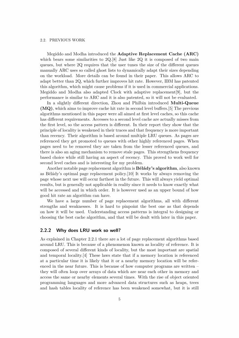
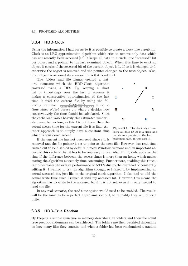
Using the information I had access to it is possible to create a clock-like algorithm.Clock is an LRU approximation algorithm which tries to remove only data whichhas not recently been accessed.[16] It keeps all data in a circle, one ”accessed” bitper object and a pointer to the last examined object. When it is time to evict anobject it checks if the accessed bit of the current object is 1. If so it is changed to 0,otherwise the object is removed and the pointer changed to the next object. Also,if an object is accessed its accessed bit is 0 it is set to 1.

Figure 3.1. The clock algorithmkeeps all data (A-J) in a circle andmaintains a pointer to the lastexamined data, in this case B.

The folders and file names created a nat-ural structure which the HDD-Clock algorithmtraversed using a DFS. By keeping a shortlist of timestamps over the last k accesses itmakes a conservative approximation of the lasttime it read the current file by using the fol-lowing formula: <cache size>

<approximate tile size>×k × c× <time since oldest access >, where c decides howconservatively the time should be calculated. Sincethe cache load varies heavily this estimated time willalso vary, but as long as this t is not lower than theactual access time for the current file it is fine. An-other approach is to simply have a constant timewhich is considered recent.

If the current file has not been read since t it isremoved and the file pointer is set to point at the next file. However, last read timeturned out to be disabled by default in most Windows versions and an important as-pect of this cache is that it has to be very easy to use. Also, NTFS only updates thetime if the difference between the access times is more than an hour, which makestesting the algorithm extremely time-consuming. Furthermore, enabling this times-tamp decreases the overall performance of NTFS due to the overhead of constantlyediting it. I wanted to try the algorithm though, so I faked it by implementing anactual accessed bit, just like in the original clock algorithm. I also had to add theactual write time since I ruined it with my accessed bit. However, this means thealgorithm has to write to the accessed bit if it is not set, even if it only needed toread the file.

In any real scenario, the read time option would need to be enabled. The resultswill be the same as for a perfect approximation of t, so in reality they will differ alittle.

3.3.5 HDD-True Random

By keeping a simple structure in memory describing all folders and their file counttrue pseudo-randomness can be achieved. The folders are then weighted dependingon how many files they contain, and when a folder has been randomized a random

13

CHAPTER 3. TESTING METHODOLOGY

file is removed in the same fashion as HDD-Random. Another way of achievingthis is to simply store all the files in a single folder, but this can cause seriousperformance issues as well as making it hard to manually browse the files. Thisalgorithm was mostly created because I was curious how the skewed randomness ofHDD-Random affected the hit rate.

3.3.6 HDD-LRU with batch removal

If the system has the last access time enabled (iOS and Android both do per default,Windows does not) the algorithm could be entirely hard drive-based until it is timeto remove data. When more room is needed it could load the last access time of allfiles in the cache, order them and remove the x% least recently accessed files, wherex can be configured to taste. For extra performance, it could also pre-emptivelydelete some files if the cache is almost full and the system is not used, for exampleat night. This will have a slightly lower hit rate than LRU, due to the fact that thecache on average will not be entirely full. When testing this I deleted 10% of thecache contents when it was full. Since this algorithm needs to read the metadata ofall files in the cache it is not suitable for large caches.

3.3.7 HDD-backed memory algorithm

Pick a memory algorithm of choice, but save only the header for each tile in memory.The data is instead saved on disk and a pointer to it is maintained in memory. Thisapproach can create huge memory overhead for regular systems due to their immensestorage capabilities, but for a mobile system it is not as big a problem. Also, sincetheir secondary storage is much faster they can use this single, unified cache insteadof two separate ones. MQ would be an excellent pick for this algorithm, but withoutthe ghost list as it is suddenly just as expensive (in terms of memory) to keep aghost as it is to keep a normal data entry.

This will have the slightly lower hit rate than the memory algorithm on mostfile systems due to file sizes being rounded up to the nearest cluster size, but otherthan that it will work just like the regular algorithm. For my tiles and partitioning,the hard drive part is approximately 100 times larger than the memory part if MQis used.

One problem with this kind of cache is how to keep the data when the cache isrestarted. One could traverse the entire cache directory and load only the metadatarequired (generally filename, size and last write time), but this is going to be veryslow for larger caches. Another option is to write a file with the data to load, justlike pre-loading is done in Chapter 5.1.2, but this is also slow for big caches. A thirdoption is to not populate the memory part with anything, but instead load the datafrom the disk when it is accessed but not available in memory. This algorithmis more complex and sensitive, but for larger caches or when a very fast start isrequired this algorithm might be the best solution. In order to get this to workproperly the algorithm for choosing which file is removed has to be modified slightly:

14

3.3. PROPOSED ALGORITHMS

before deleting files which have memory metadata the cache folder is traversed (justlike HDD-Clock in Chapter 3.3.4, except instead of the Accessed bit it checks thememory cache) and files which are not in the memory index are deleted. Once theend is reached the normal deletion algorithm takes over and the cache does not haveto check the hard drive every time it thinks it does not contain a file. For the test Iimplemented the first version, but as long as they are all loaded in the same orderthey will get the same hit rate. Version one and three will be in the same order, butby making version two preserve the LRU order it could get a very small increase inhit rate.

15

Chapter 4

Analysis of test data

In this chapter I put my test data through some tests to see if it exhibits any of thetypical patterns for cache traces.

4.1 Data sources

I have two proper data sources: the first is 739 851 consecutive accesses from hitta.se(hitta). They provide a service which allows anyone to search for people or busi-nesses and display them on a map, or just browse the map. The second is 452 104consecutive accesses from Ragn-Sells, who deliver recycling material (ragnsells).This is a closed service and the trucks move along predetermined paths. I also use asubset of Ragn-Sells, consisting of 100 000 accesses (ragn100) to test how the cachebehaves in short term usage.

4.2 Pattern analysis

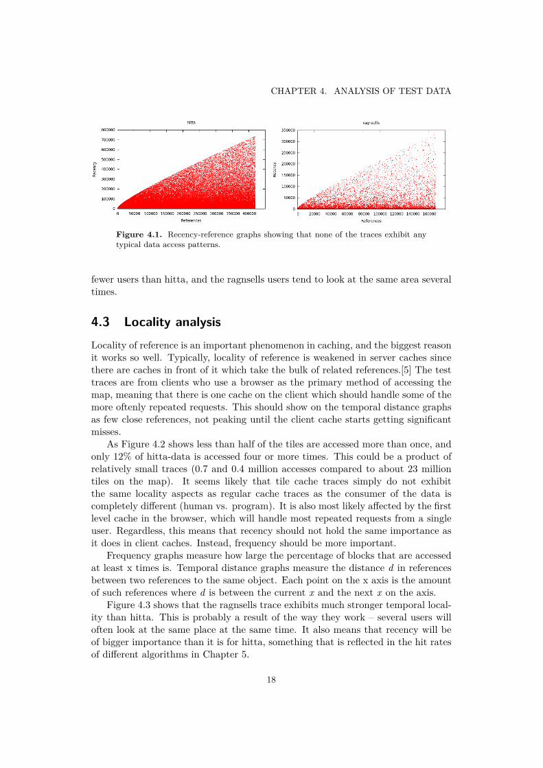
In classic caching, loops and scans are a typical component of any real data set.However, map lookups do not exhibit the same patterns as programs do. It wouldmake sense to see some scanning patterns though, when users look around on themap. I’ve made recency-reference graphs for the data. This type of graph is made byplotting how many other references are made between references to the same objectover time. Also, very close references seldom give any important information sothe most recent 1000 references are ignored. Horizontal lines in the graphs indicatestandard loops. Steep upwards diagonals are objects re-accessed in the oppositeorder, also common in loops. Both of these could also appear if a user scanned aportion of the map and then went back to scan it again.

As the scatter plots in Figure 4.1 show the data contains no loops and showno distinct access patterns. Interestingly though, the low density in the upper partof the plot show that the ragnsells trace exhibits stronger locality than the hittatrace. This is probably because the ragnsells was gathered over longer time with

17

CHAPTER 4. ANALYSIS OF TEST DATA

Figure 4.1. Recency-reference graphs showing that none of the traces exhibit anytypical data access patterns.

fewer users than hitta, and the ragnsells users tend to look at the same area severaltimes.

4.3 Locality analysisLocality of reference is an important phenomenon in caching, and the biggest reasonit works so well. Typically, locality of reference is weakened in server caches sincethere are caches in front of it which take the bulk of related references.[5] The testtraces are from clients who use a browser as the primary method of accessing themap, meaning that there is one cache on the client which should handle some of themore oftenly repeated requests. This should show on the temporal distance graphsas few close references, not peaking until the client cache starts getting significantmisses.

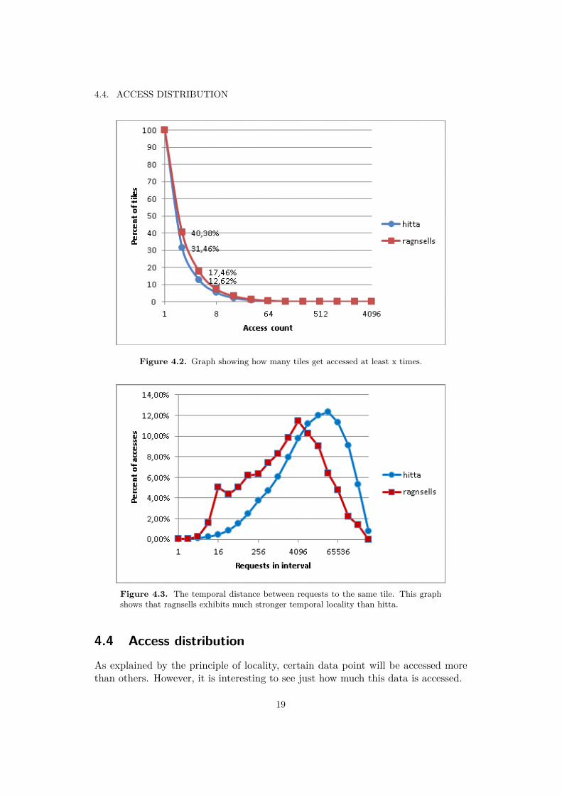
As Figure 4.2 shows less than half of the tiles are accessed more than once, andonly 12% of hitta-data is accessed four or more times. This could be a product ofrelatively small traces (0.7 and 0.4 million accesses compared to about 23 milliontiles on the map). It seems likely that tile cache traces simply do not exhibitthe same locality aspects as regular cache traces as the consumer of the data iscompletely different (human vs. program). It is also most likely affected by the firstlevel cache in the browser, which will handle most repeated requests from a singleuser. Regardless, this means that recency should not hold the same importance asit does in client caches. Instead, frequency should be more important.

Frequency graphs measure how large the percentage of blocks that are accessedat least x times is. Temporal distance graphs measure the distance d in referencesbetween two references to the same object. Each point on the x axis is the amountof such references where d is between the current x and the next x on the axis.

Figure 4.3 shows that the ragnsells trace exhibits much stronger temporal local-ity than hitta. This is probably a result of the way they work – several users willoften look at the same place at the same time. It also means that recency will beof bigger importance than it is for hitta, something that is reflected in the hit ratesof different algorithms in Chapter 5.

18

4.4. ACCESS DISTRIBUTION

Figure 4.2. Graph showing how many tiles get accessed at least x times.

Figure 4.3. The temporal distance between requests to the same tile. This graphshows that ragnsells exhibits much stronger temporal locality than hitta.

4.4 Access distributionAs explained by the principle of locality, certain data point will be accessed morethan others. However, it is interesting to see just how much this data is accessed.

19

CHAPTER 4. ANALYSIS OF TEST DATA

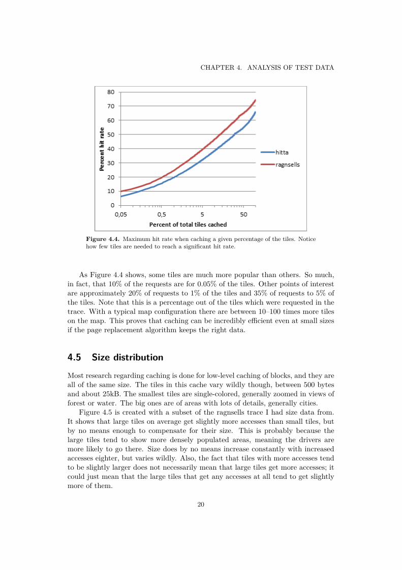
Figure 4.4. Maximum hit rate when caching a given percentage of the tiles. Noticehow few tiles are needed to reach a significant hit rate.

As Figure 4.4 shows, some tiles are much more popular than others. So much,in fact, that 10% of the requests are for 0.05% of the tiles. Other points of interestare approximately 20% of requests to 1% of the tiles and 35% of requests to 5% ofthe tiles. Note that this is a percentage out of the tiles which were requested in thetrace. With a typical map configuration there are between 10–100 times more tileson the map. This proves that caching can be incredibly efficient even at small sizesif the page replacement algorithm keeps the right data.

4.5 Size distribution

Most research regarding caching is done for low-level caching of blocks, and they areall of the same size. The tiles in this cache vary wildly though, between 500 bytesand about 25kB. The smallest tiles are single-colored, generally zoomed in views offorest or water. The big ones are of areas with lots of details, generally cities.

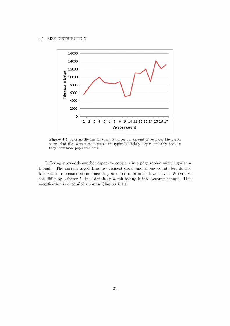
Figure 4.5 is created with a subset of the ragnsells trace I had size data from.It shows that large tiles on average get slightly more accesses than small tiles, butby no means enough to compensate for their size. This is probably because thelarge tiles tend to show more densely populated areas, meaning the drivers aremore likely to go there. Size does by no means increase constantly with increasedaccesses eighter, but varies wildly. Also, the fact that tiles with more accesses tendto be slightly larger does not necessarily mean that large tiles get more accesses; itcould just mean that the large tiles that get any accesses at all tend to get slightlymore of them.

20

4.5. SIZE DISTRIBUTION

Figure 4.5. Average tile size for tiles with a certain amount of accesses. The graphshows that tiles with more accesses are typically slightly larger, probably becausethey show more populated areas.

Differing sizes adds another aspect to consider in a page replacement algorithmthough. The current algorithms use request order and access count, but do nottake size into consideration since they are used on a much lower level. When sizecan differ by a factor 50 it is definitely worth taking it into account though. Thismodification is expanded upon in Chapter 5.1.1.

21

Chapter 5

Results

In this chapter I present the test results and discuss the implications they have.

5.1 Memory cache

Size (MB) 10 50 100 150 250 500 1000hitta (max 66.04% hit rate)

LRU 8.21 20.17 28.55 34.30 42.26 53.55 62.71MQ 10.95 24.69 33.05 38.69 46.10 55.20 62.27MQ-S 10.02 23.68 32.08 37.76 45.24 54.48 61.81ARC 12.54 25.66 34.25 40.24 48.08 56.59 63.45FIFO 7.18 18.09 25.69 31.01 38.50 49.33 59.40LFU 10.00 18.65 25.85 33.39 41.42 53.18 62.55LFU-A 8.96 22.80 30.00 35.03 41.90 53.37 62.10LFU-S-A 9.57 20.63 28.00 33.18 40.60 52.41 62.442Q 10.54 22.46 30.46 35.89 43.18 52.30 56.89

ragnsells (max 74.49% hit rate)LRU 26.05 47.21 58.12 63.86 69.18 73.39 74.49MQ 27.92 47.52 57.18 62.56 67.82 72.72 74.49MQ-S 27.93 47.89 57.37 62.68 67.66 72.58 74.49ARC 10.93 28.06 56.23 61.07 68.97 73.27 74.49FIFO 24.48 44.07 54.72 60.71 66.66 72.39 74.49LFU 5.83 9.87 16.48 32.65 54.01 66.97 74.46LFU-A 11.55 26.74 26.30 35.02 54.55 67.68 74.46LFU-S-A 3.38 10.65 14.67 22.08 42.60 63.71 74.492Q 26.44 46.81 55.53 60.41 65.23 68.39 70.03

Table 5.1. Results from the memory tests. The best results are in bold.

For hitta, these results mirror the ones Megiddo and Modha received in their

23

CHAPTER 5. RESULTS

tests[15], though the 2Q algorithm performs under expectations. I suspect thisis either due to different configuration of the constants (I used the constants theauthors recommended) or simply due to differences in data.

The ragnsells trace gives more interesting results with big differences between thealgorithms. There are two very noticeable groupings in there: group 1 containingthe LFU based algorithms and for smaller sizes ARC, and group 2 with LRU,MQ, MQ-S, 2Q and FIFO. My hypothesis is that the reason for this is the strongtemporal locality in the ragnsells trace. All algorithms in group 2 have strongrecency aspects: FIFO and LRU are built around recency and MQ depends highlyon recency. Especially so at small sizes, simply because it will not contain tileslong enough for them to get many hits. The LFU based algorithms in group 1 arealmost purely frequency dependent and will miss a lot because of this. ARC ismore recency-based and does join group 2 for cache sizes ≥ 100MB, but the lowperformance at smaller sizes is unexpected. Ragnsells has both strong temporallocality and some tiles with a lot of hits, and this probably confuses the adaptionalgorithm at small cache sizes, increasing the size of the second queue when it shouldhave done the opposite.

Interestingly, the classic LRU algorithm which was shadowed by more advancedalgorithms for the hitta trace shines here. This goes to show just how important theenvironment is for the algorithm choice, and that even a simple algorithm such asLRU can still compete with more modern algorithms under the right circumstances.

5.1.1 The size modification

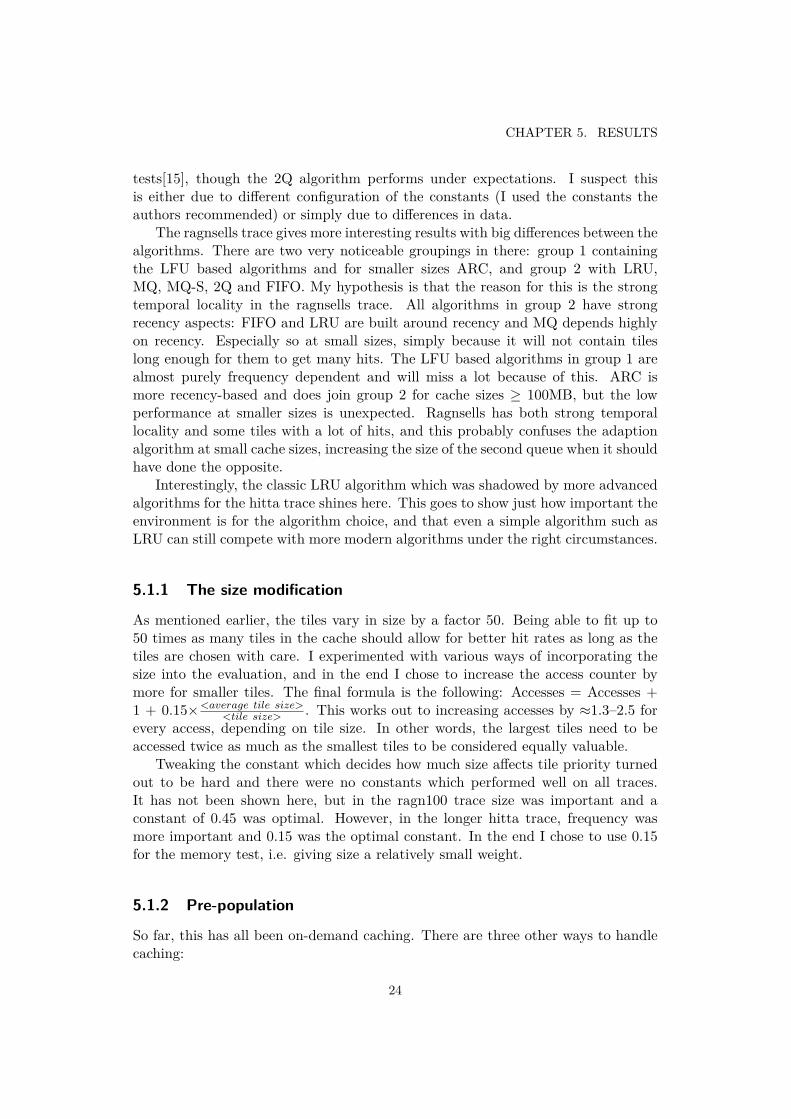
As mentioned earlier, the tiles vary in size by a factor 50. Being able to fit up to50 times as many tiles in the cache should allow for better hit rates as long as thetiles are chosen with care. I experimented with various ways of incorporating thesize into the evaluation, and in the end I chose to increase the access counter bymore for smaller tiles. The final formula is the following: Accesses = Accesses +1 + 0.15×<average tile size>

<tile size> . This works out to increasing accesses by ≈1.3–2.5 forevery access, depending on tile size. In other words, the largest tiles need to beaccessed twice as much as the smallest tiles to be considered equally valuable.

Tweaking the constant which decides how much size affects tile priority turnedout to be hard and there were no constants which performed well on all traces.It has not been shown here, but in the ragn100 trace size was important and aconstant of 0.45 was optimal. However, in the longer hitta trace, frequency wasmore important and 0.15 was the optimal constant. In the end I chose to use 0.15for the memory test, i.e. giving size a relatively small weight.

5.1.2 Pre-population

So far, this has all been on-demand caching. There are three other ways to handlecaching:

24

5.1. MEMORY CACHE

• Pre-populating it with objects which are thought to be important. This isoften done in a static fashion – the starting population of the cache is con-figured to values which are known to be good. If the cache always keeps thisstatic data it is called static caching. This can give good results for very smallcaches which would otherwise throw away good data too fast.

• Predict which objects will be loaded ahead of time. This can waste a lotof time if done wrong, but if the correct data is loaded response time candecrease greatly. Also, if objects are loaded during times when the load islow, throughput can be increased during high load times thanks to higher hitrate.

• Pre-populating with objects based on some dynamic algorithm which takesrecent history into account.

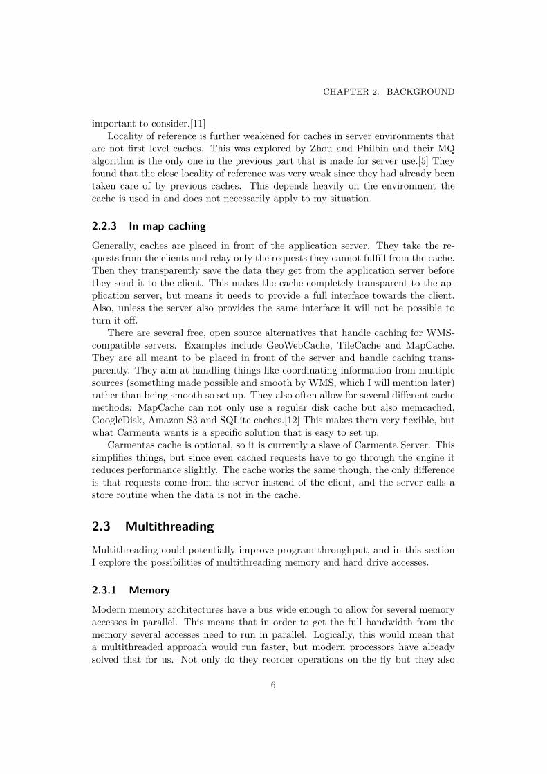
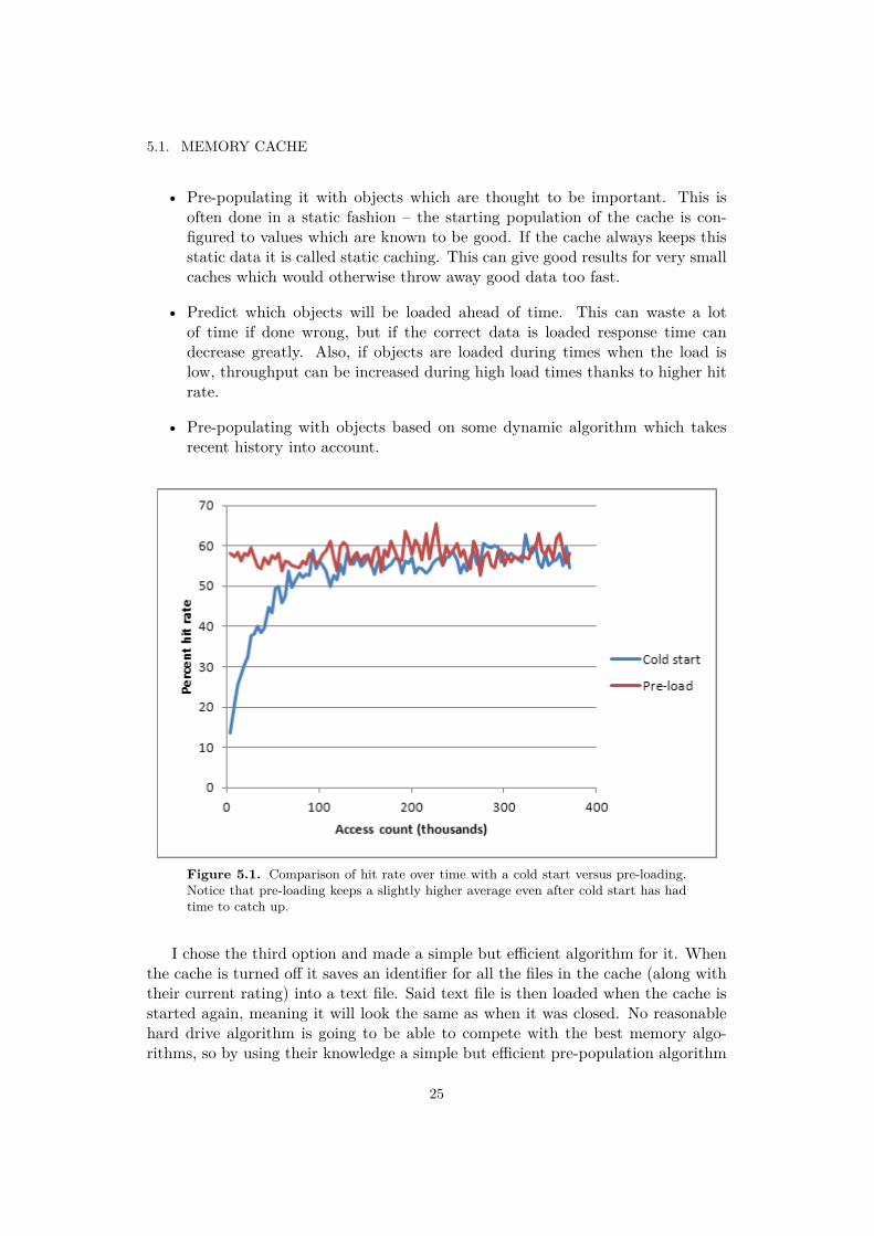
Figure 5.1. Comparison of hit rate over time with a cold start versus pre-loading.Notice that pre-loading keeps a slightly higher average even after cold start has hadtime to catch up.

I chose the third option and made a simple but efficient algorithm for it. Whenthe cache is turned off it saves an identifier for all the files in the cache (along withtheir current rating) into a text file. Said text file is then loaded when the cache isstarted again, meaning it will look the same as when it was closed. No reasonablehard drive algorithm is going to be able to compete with the best memory algo-rithms, so by using their knowledge a simple but efficient pre-population algorithm

25

CHAPTER 5. RESULTS

is achieved. The biggest downside with this algorithm is that it does not work thefirst time around. In order to have it work the first time the first option needs tobe used – static caching. It requires more configuration though, and I do not feel itis worth it for the small performance increase.

For Figure 5.1, I split hitta into two equal halves. The reason I did this is becausein a real world situation the same long trace is extremely unlikely to be repeated,and it would give the algorithm an unrealistic advantage since it knows beforehandwhich tiles are often accessed. Their max hit rate are 59.04% for the cold startversion and 57.88% for the pre-loaded one, so the hit rates are comparable.

As expected, the hit rate for pre-loading starts off approximately where it leftoff. However, it also continues to have a slightly higher hit rate on average throughthe entire trace. At around 25% cold start has caught up with pre-loading, buteven then hit rate is still slightly lower – 56.23% on average from 25% – 100% ofthe trace compared to 58.20% for the pre-loaded one (total averages are 52.64% forcold start and 57.79% for pre-loading). The pre-loaded one won despite having aworse max hit rate than the cold start trace – it even achieved a hit rate higherthan the max theorical limit for a cold start since it did not have to miss every tilebefore loading it.

26

5.2. HARD DRIVE CACHE

5.1.3 Speed

All algorithms are O(1) except LFU and its variations, which are O(log(n)). Thismeans speeds should be similar, but some algorithms are definitely more complexthan others which could result in higher constants. When running the tests I tookall the precautions mentioned in Chapter 3.1.2 and also ran the test on both Inteland AMD, but all the graphs looked the same. The only thing that differed wasthe magnitude of the run times, otherwise memory-limited Intel, processor-limitedIntel and memory-limited AMD are all almost identical.

Figure 5.2. Result of speed run where the CPU was the limiting factor. There areobviously no big constants hidden in the Ordo notation.

All algorithms except LFU are remarkably close in execution time; the differenceis only a few seconds. In other words, there are no huge hidden constants in theOrdo notation.

5.2 Hard drive cache

As Table 5.2 shows, performance follows overhead pretty closely and the differencesare overall very small. HDD-Random performs surprisingly well – it is almost asgood as memory FIFO (see Table 5.1). This is impressive, especially consideringthat the hard drive algorithms have to deal with cluster size overhead. 4kB clustersize is the default for modern NTFS drives, meaning that file sizes are rounded upto the nearest 4kB. This gives an overhead of approximately 20% with the currenttiles.

27

CHAPTER 5. RESULTS

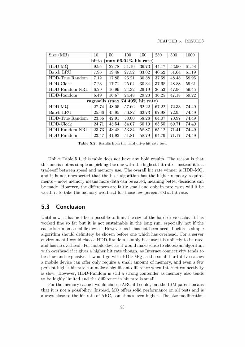
Size (MB) 10 50 100 150 250 500 1000hitta (max 66.04% hit rate)

HDD-MQ 9.95 22.78 31.10 36.73 44.17 53.90 61.58Batch LRU 7.96 19.48 27.52 33.02 40.62 51.64 61.19HDD-True Random 7.12 17.85 25.21 30.38 37.59 48.48 58.95HDD-Clock 7.23 17.71 25.04 30.34 37.68 48.88 59.61HDD-Random NRU 6.29 16.99 24.32 29.19 36.53 47.96 59.45HDD-Random 6.49 16.67 24.48 29.23 36.25 47.18 59.22

ragnsells (max 74.49% hit rate)HDD-MQ 27.74 48.05 57.66 62.22 67.22 72.33 74.49Batch LRU 25.66 45.95 56.82 62.73 67.98 72.95 74.49HDD-True Random 23.56 42.91 53.00 58.28 64.07 70.97 74.49HDD-Clock 24.71 43.54 54.07 60.10 65.55 69.71 74.49HDD-Random NRU 23.73 43.48 53.34 58.87 65.12 71.41 74.49HDD-Random 23.47 41.93 51.81 58.79 64.79 71.17 74.49

Table 5.2. Results from the hard drive hit rate test.

Unlike Table 5.1, this table does not have any bold results. The reason is thatthis one is not as simple as picking the one with the highest hit rate – instead it is atrade-off between speed and memory use. The overall hit rate winner is HDD-MQ,and it is not unexpected that the best algorithm has the higher memory require-ments – more memory means more data can be saved, meaning better decisions canbe made. However, the differences are fairly small and only in rare cases will it beworth it to take the memory overhead for those few percent extra hit rate.

5.3 ConclusionUntil now, it has not been possible to limit the size of the hard drive cache. It hasworked fine so far but it is not sustainable in the long run, especially not if thecache is run on a mobile device. However, as it has not been needed before a simplealgorithm should definitely be chosen before one which has overhead. For a serverenvironment I would choose HDD-Random, simply because it is unlikely to be usedand has no overhead. For mobile devices it would make sense to choose an algorithmwith overhead if it gives a higher hit rate though, as Internet connectivity tends tobe slow and expensive. I would go with HDD-MQ as the small hard drive cachesa mobile device can offer only require a small amount of memory, and even a fewpercent higher hit rate can make a significant difference when Internet connectivityis slow. However, HDD-Random is still a strong contender as memory also tendsto be highly limited and the difference in hit rate is small.

For the memory cache I would choose ARC if I could, but the IBM patent meansthat it is not a possibility. Instead, MQ offers solid performance on all tests and isalways close to the hit rate of ARC, sometimes even higher. The size modification

28

5.4. FUTURE WORK

of MQ happened to beat both MQ and ARC in the small ragnsells tests, but overallit is not as good as regular MQ.

5.4 Future workThe size modification mentioned in Chapter 5.1.1 uses a constant which is hard totweak without knowing the exact environment the algorithm will be used in. Also,the hit rate can probably be improved by changing this value over time. MQ usesa ghost list which gives information on which tiles have been deleted – it could beused in a manner similar to how ARC uses it to tweak this constant.

29

Bibliography

[1] G. Gagne A. Silberschatz, P. B. Galvin. Operating Systems Concepts. Seventhedition, 2005.

[2] A. S. Tanenbaum. Modern Operating System. Prentice-Hall, 1992.

[3] T. Johnson and D. Shasha. 2q: A low overhead high performance buffer man-agement replacement system, 1994.

[4] P. J. Denning. The locality principle. Communication Networks and ComputerSystems, pages 43–67, 2006.

[5] Y. Zhou and J. F. Philbin. The multi-queue replacement algorithm for secondlevel buffer caches, 2001.

[6] D. Matani K. Shah, A. Mitra. An o(1) algorithm for implementing the lfucache eviction scheme, 2010.

[7] G. Weikum E. J. O’Neil, P. E. O’Neill. The lru-k page replacement algorithmfor database disk buffering, 1993.

[8] N. Megiddo and D. Modha. Arc: A self-tuning, low overhead replacementcache, 2003.

[9] N. Megiddo and D. Modha. Car: Clock with adaptive replacement, 2004.

[10] L. A. Bélády. A study of replacement algorithms for a virtual-storage computer,1966.

[11] M. Snir and J. Yu. On the theory of spatial and temporal locality, 2005.

[12] Thomas Bonfort. Cache types for mapcache(http://mapserver.org/trunk/mapcache/caches.html). Accessed 2012-05-16.

[13] Opengis web map service (wms) implementation specification, 2006.

[14] Wms tile caching (http://wiki.osgeo.org/wiki/wms_tile_caching). Accessed2012-03-02.

31

BIBLIOGRAPHY

[15] N. Megiddo and D. Modha. Outperforming lru with an adaptive replacementcache algorithm. IEEE Computer Magazine, pages 58–65, 2004.

[16] F. J. Corbato. A paging experiment with the multics system, 1969.

32

TRITA-CSC-E 2012:073 ISRN-KTH/CSC/E--12/073-SE

ISSN-1653-5715

www.kth.se