Evaluation of Numerical Variable ... - ubibliorum.ubi.pt§ão... · UNIVERSIDADE DA BEIRA INTERIOR...
123
UNIVERSIDADE DA BEIRA INTERIOR Engenharia Evaluation of Numerical Variable Density Approach to Cryogenic Jets Eduardo Luís Santos Farias Antunes Dissertação para obtenção do Grau de Mestre em Engenharia Aeronáutica (2º ciclo de estudos) Orientador: Professor Doutor Jorge Manuel Martins Barata Covilhã, Junho de 2011
Transcript of Evaluation of Numerical Variable ... - ubibliorum.ubi.pt§ão... · UNIVERSIDADE DA BEIRA INTERIOR...

UNIVERSIDADE DA BEIRA INTERIOR Engenharia
Evaluation of Numerical Variable Density
Approach to Cryogenic Jets
Eduardo Luís Santos Farias Antunes
Dissertação para obtenção do Grau de Mestre em
Engenharia Aeronáutica (2º ciclo de estudos)
Orientador: Professor Doutor Jorge Manuel Martins Barata
Covilhã, Junho de 2011

Eduardo Luís Santos Farias Antunes
ii
Evaluation of Numerical Variable Density Approach to Cryogenic Jets
iii
Agradecimentos
Quero agradecer ao meu orientador, Professor Doutor Jorge Manuel Martins Barata, pelas excelentes aulas de Propulsão 1 onde aprendi muito e ganhei ainda maior paixão pela área, pela oportunidade que me deu de trabalhar com ele e pelo enorme conhecimento, ajuda e encorajamento que me prestou. Quero agradecer ao Professor Doutor André Resende Rodrigues da Silva, pela ajuda e apoio que me prestou durante a execução desta tese principalmente na documentação e apoio bibliográfico. Quero agradecer ao Engenheiro Fernando Manuel Silva Pereira Neves pela disponibilidade,
apoio e encorajamento que me prestou principalmente durante a minha fase de
aprendizagem.
Quero agradecer a todos os meus amigos e colegas, pelo apoio moral, encorajamento e
conhecimento que me prestaram durante todo o meu percurso académico.
Por último, mas não menos importante, quero agradecer a toda a minha família, em especial,
aos meus pais e irmã por sempre me terem apoiado e acreditado em mim
incondicionalmente.
Eduardo Antunes
Covilhã 2011

Eduardo Luís Santos Farias Antunes
iv
Evaluation of Numerical Variable Density Approach to Cryogenic Jets
v
Resumo
O presente trabalho dedica-se ao estudo de jactos de azoto líquido criogênico em condições
subcríticas perto do ponto crítico. A injecção de combustível é um dos maiores desafios
actuais na engenharia de motores diesel, turbinas de gás e motores de foguete, com a
complexidade extra de nestes últimos se combinar também a injecção de comburente. É
amplamente conhecido que o aumento das pressões e temperaturas de operação aumenta a
eficiências dos motores e reduz o consumo específico. Assim, existe a tendência de um
aumento generalizado das pressões de operação em motores modernos. No entanto elevadas
pressões de operação na câmara de combustão têm como consequência a exposição dos
fluidos a condições que excedem os valores críticos. Vários autores concluíram que nestas
condições os fluidos injectados sofrem variações nas suas propriedades que levam a que os
modelos tradicionais de escoamentos com duas fases não consigam modelar correctamente o
comportamento do jacto, assim são precisos novos modelos computacionais para estas
condições específicas. Barata et al. [18] realizaram uma investigação numérica com o intuito
de avaliar a aplicabilidade do modelo de gases de densidade variável em jactos líquidos em
condições sub e supercríticas. Os resultados de Barata et al. [18] revelaram uma boa
concordância com os dados experimentais, mas apenas foram consideradas razões de
densidade intermédias de 0.05 a 0.14. O objectivo do presente trabalho é o de estender as
investigações de Ref. 18 a razões de densidades mais baixas entre 0.025 e 0.045 que
correspondem a casos de pressões subcríticas da câmara de injecção e determinar o limite de
aplicabilidade do modelo de gases de densidade variável. Os resultados obtidos estão em
concordância com os dados experimentais e numéricos obtidos por Chehroudi et al.
apresentados em Ref. 18. Neste trabalho verificou-se também que o modelo computacional
usado não oferece resultados validos para razões de densidade abaixo de 0.025 identificando-
se assim o limite de aplicabilidade do modelo de gases de densidade variável.
Palavras-chave
Injecção de combustível; ponto crítico; condições supercríticas; motores foguete; motores diesel; razão de densidades; jactos; densidade variável.

Eduardo Luís Santos Farias Antunes
vi

Evaluation of Numerical Variable Density Approach to Cryogenic Jets
vii
Resumo alargado
A injecção de combustível apresenta-se como um dos maiores desafios actuais da
engenharia em motores diesel, turbinas de gás e foguetes, sendo que neste ultimo caso se
acrescenta ainda a complexidade extra da injecção combinada de oxidante. Estudos
experimentais e numéricos efectuados para vários tipos de motores têm vindo a demonstrar
que o aumento da pressão de funcionamento dos mesmos aumenta bastante a sua eficiência e
reduz o consumo específico. Assim antevê-se que seja de todo o interesse a continuação do
aumento das pressões de operação dos motores, o que, com o aparecimento de materiais
inovadores mais resistentes, faz crescer ainda mais esta tendência.
No entanto, o aumento da pressão de funcionamento leva a que se atinjam e se
ultrapassem os pontos críticos de pressão e temperatura dos líquidos e gases envolvidos.
Como exemplos, a câmara de combustão do motor principal do Space Shuttle atinge uma
pressão de 22.3 MPa enquanto no motor Vulcain, usado no Ariane 5, se registou um valor
recorde de 28.2 MPa [1]. Em qualquer dos casos as pressões na câmara de combustão
ultrapassam a pressão critica de Pcr = 5.043 MPa para o oxigénio liquido e Pcr = 1.28 MPa do
hidrogénio liquido. Também em motores diesel a câmara combustão pode em alguns casos
atingir o dobro da pressão crítica. Para aplicações em motores foguete a temperatura inicial
do oxigénio injectado está abaixo do valor crítico (Tcr = 154.58 K), mas assim que este entra
na câmara de combustão passa por uma transição na qual atinge temperaturas supercríticas.
Nestas condições diz-se que o combustível (ou comburente líquido) está em condições
supercríticas e o seu estado físico passa a ser denominado de estado fluido [1]. Á medida que
o fluido alcança condições de pressão e temperatura que ultrapassam os valores críticos, o
fluido passa por alterações significativas nas suas propriedades. A difusibilidade mássica
efectiva, a tensão superficial e o calor latente do líquido desaparecem em condições
supercríticas. Por outro lado, o calor específico a pressão constante, Cp, a compressibilidade
isentrópica, κs, e a condutividade térmica, λ, tornam-se infinitos [2]. Estas mudanças de
comportamento do fluido fazem com que os tradicionais modelos de escoamentos com duas
fases não possam ser aplicados em injecções de combustível em condições supercríticas.
Desta forma, nasce a necessidade de desenvolver novos modelos computacionais que possam
ser correctamente aplicado à injecção de combustível em condições supercríticas.
Vários autores investigaram a injecção de combustível em condições supercríticas tanto
experimentalmente como numericamente [3-22]. As primeiras investigações experimentais
realizadas tinham como principal objectivo o estudo da estrutura visual do jacto, sem a
obtenção de quaisquer resultados quantitativos [1, 6]. Estas investigações verificaram que a
estrutura do jacto se alterava significativamente com o aumento da pressão. Primeiro a
redução da tensão superficial leva à formação de ligamentos no jacto e de gotas de fluido que
se separam da estrutura principal do jacto, um aumento maior da pressão da câmara de
injecção para condições supercríticas conduz a uma estrutura do jacto semelhante àquela que

Eduardo Luís Santos Farias Antunes
viii
seria visível numa injecção de um gás num ambiente também gasoso. Trabalhos
experimentais mais recentes levaram a cabo estudos quantitativos nos quais foram obtidos
resultados sobre o ângulo de abertura do jacto, densidade e temperatura [4, 7, 15, 16]. Estes
resultados quantitativos experimentais permitem a comparação com os resultados obtidos em
estudos numéricos e através da comparação é feita a validação destes mesmos modelos
numéricos [17-22].
Barata et al. [18] realizou uma investigação inicial com o objectivo de avaliar as
capacidades de um modelo computacional desenvolvido para escoamentos incompressíveis
mas com densidade variável quando aplicado a condições supercríticas. Os resultados
alcançados mostram ser concordantes com os dados experimentais, no entanto, nesta
investigação apenas foram considerados razões de densidade intermédias de 0.05 a 0.14.
O presente trabalho teve como principal objectivo estender a investigação da Ref. 18 a
menores razões de densidade e definir qual o limite mínimo de razão de densidade para o
qual se podia aplicar o modelo de escoamento incompressível mas com densidade variável.
Para isso testaram-se diferentes razões de densidades abaixo de 0.05. Testaram se as razões
de densidade ω = 0.010, 0.015, 0.020, 0.025, 0.035 e 0.045. Para estas razões de densidades
obtiveram-se os campos escalares e da velocidade, gráficos da variação axial da densidade na
linha central, do decaimento axial de velocidade na linha central e finalmente da metade da
largura do meio da velocidade máxima (HWHMV) o qual permitiu determinar a tangente do
ângulo de abertura do jacto.
A analise dos gráficos permitiu concluir que o modelo de gases de densidade variável
resultados bastante concordantes com outros trabalhos para razões de densidades de 0.025 a
0.045. No entanto definiu-se que o modelo deixa de ser aplicável para razões de densidade
inferiores a 0.025.
Um breve estudo, sobre a influência da velocidade de injecção sobre o comportamento
obtido para o jacto no presente modelo, concluiu que a velocidade de injecção influência os
resultados obtidos sobre o comportamento do jacto e desta forma deve ser um parâmetro a
ter em conta.
Evaluation of Numerical Variable Density Approach to Cryogenic Jets
ix
Abstract
The present work is devoted to study cryogenic nitrogen jets in high subcritical conditions.
Fuel injection is one of the great challenges in engineering of diesel engines, gas turbines and
rocket engines, combining in the last one also the injection of oxidizer. It is widely known
that the increase of operation pressures and temperatures increases engine efficiency and
reduces fuel specific consumption. Thus, it is a general trend in modern engines the operation
in increasingly higher pressures. However at higher chamber pressures the injected fluids may
experience ambient conditions exceeding the critical values. Several authors stated that at
these conditions the injected fluids suffers a change of its properties, and the traditional two-
phase flow models cannot correctly predict the jet behavior at these conditions, thus new
computational models are needed for these specific conditions. Barata et al. [18] performed
a numerical investigation aimed to evaluate the applicability of an incompressible but
variable density model in liquid jets under sub-to-supercritical conditions. The results
achieved agree well with the experimental data but they only considered intermediate
density ratios from 0.05 to 0.14. The objective of the present work was to extend the
investigation of Ref. 18 to lower density ratios from 0.025 to 0.045 which correspond to cases
with subcritical chamber pressures. The obtained results agree well with the experimental
and numerical data of Chehroudi et al. presented in Ref. 18. It was also found in this work
that the computational model does not offers valid results for density ratios bellow 0.025,
thus identifying the limit of applicability of model.
Keywords
Fuel injection; critical point; supercritical conditions; rocket engines; diesel engines; density ratio; jets; variable density.

Eduardo Luís Santos Farias Antunes
x
Evaluation of Numerical Variable Density Approach to Cryogenic Jets
xi
Index
Agradecimentos ............................................................................................................. iii
Resumo ............................................................................................................................. v
Resumo alargado .......................................................................................................... vii
Abstract .......................................................................................................................... ix
Index ................................................................................................................................ xi
Figures list .................................................................................................................... xiii
Tables list ...................................................................................................................... xv
Nomenclature ............................................................................................................. xvii
X/D = axial distance normalized by injector diameter .................................... xvii
Acronyms List ............................................................................................................... xix
Chapter 1 ......................................................................................................................... 1
Introduction .................................................................................................................... 1
Chapter 2 ....................................................................................................................... 19
Mathematical Model .................................................................................................... 19
2.1 Governing Equations ......................................................................................... 19
2.2 Numerical Method ............................................................................................. 21
2.3 Boundary Conditions ......................................................................................... 21
Chapter 3 ....................................................................................................................... 23
Results and Discussion ................................................................................................. 23
Introduction .............................................................................................................. 23
3.1 Study of the density ratio influence .............................................................. 24
3.1.1 Velocity and scalar fields for ω = 0.025, 0.035 and 0.045 ................. 26
3.1.2 Axial variation of centerline density for ω = 0.025, 0.035 and 0.045
................................................................................................................................ 33
3.1.3 Centerline velocity decay for ω = 0.025, 0.035 and 0.045 ................ 37
3.1.4 Half width of half maximum of the velocity for ω = 0.025, 0.035 and
0.045 ....................................................................................................................... 42
3.1.5 Centerline velocity and density decay rate at various chamber-to-
injectant density ratios ....................................................................................... 46
3.1.6 Tangent of the spreading angle at various chamber-to-injectant
density ratios ........................................................................................................ 47

Eduardo Luís Santos Farias Antunes
xii
3.2 Study of the injection velocity influence ...................................................... 50
3.2.1 Velocity and scalar fields for Uin = 5, 10 and 20 m.s-1 ........................ 51
3.2.2 Axial variation of the centerline velocity for Uin = 3, 5, 10 and 20
m.s-1 ........................................................................................................................ 55
3.2.3 Centerline velocity decay for Uin = 3, 5, 10 and 20 m.s-1 ................... 56
3.2.4 Half width of half maximum of the velocity for Uin = 3, 5, 10 and 20
m.s-1 ........................................................................................................................ 58
Chapter 4 ....................................................................................................................... 61
Conclusion ...................................................................................................................... 61
References ..................................................................................................................... 63
Attachment 1.....................................................................................................................
Attachment 2.....................................................................................................................
Attachment 3.....................................................................................................................
Evaluation of Numerical Variable Density Approach to Cryogenic Jets
xiii
Figures list
Figure 1– LN2 injection in GN2 at a) 4.0, b) 3.0 and c) 2.0 MPa [6]. .................................. 9
Figure 2 - Software magnified images of the jet at its outer boundary showing the transition
to the gas-jet like appearance, starting at just below the critical pressure of the injected
fluid. Images are at a fixed supercritical chamber temperature of 300 K [1]. ................... 11
Figure 3 - Flow configuration .............................................................................. 22
Figure 4 - Velocity and scalar fields of the jet with a density ratio of ω = 0.025 and a chamber
pressure of Pr = 0.583, (a) Velocity vectors, (b) Mixture fraction contours, (c) Density
contours. ...................................................................................................... 26
Figure 5 - Velocity and scalar fields of the jet with a density ratio of ω = 0.035 and a chamber
pressure of Pr = 0.642, (a) Velocity vectors, (b) Mixture fraction contours, (c) Density
contours. ...................................................................................................... 28
Figure 6 - Velocity and scalar fields of the jet with a density ratio of ω = 0.045 and a chamber
pressure of Pr = 0.825, (a) Velocity vectors, (b) Mixture fraction contours, (c) Density
contours. ...................................................................................................... 30
Figure 7 - Axial variation of the centerline density with a density ratio of ω = 0.025 and a
chamber pressure of Pr = 0.583. .......................................................................... 33
Figure 8 - Axial variation of the centerline density with a density ratio of ω = 0.035 and a
chamber pressure of Pr = 0.642. .......................................................................... 34
Figure 9 - Axial variation of the centerline density with a density ratio of ω = 0.045 and a
chamber pressure of Pr = 0.825. .......................................................................... 35
Figure 10 - Axial variation of the centerline density in a logarithmic scale for the cases 1, 2
and 3. .......................................................................................................... 36
Figure 11 - Centerline velocity decay for a density ratio of ω = 0.025 and a chamber pressure
of Pr = 0.583. ................................................................................................. 37
Figure 12 Centerline velocity decay for a density ratio of ω = 0.035 and a chamber pressure of
Pr = 0.642. .................................................................................................... 38
Figure 13 Centerline velocity decay for a density ratio of ω = 0.045 and a chamber pressure of
Pr = 0.825. .................................................................................................... 39
Figure 14 - Centerline velocity decay for the cases 1, 2 and 3 of Table 1. ....................... 41
Figure 15 - Half width of half maximum of the velocity for a density ratio of ω = 0.025 and a
chamber pressure of Pr = 0.583. .......................................................................... 42
Figure 16 - Half width of half maximum of the velocity for a density ratio of ω = 0.035 and a
chamber pressure of Pr = 0.642. .......................................................................... 43
Figure 17 - Half width of half maximum of the velocity for a density ratio of ω = 0.045 and a
chamber pressure of Pr = 0.825. .......................................................................... 44
Figure 18 - Half width of half maximum of the velocity for the cases 1, 2 and 3 of Table 1. . 46

Eduardo Luís Santos Farias Antunes
xiv
Figure 19 – Decay rate of the centerline velocity and density. ..................................... 47
Figure 20 - Tangent of the spreading angle versus the chamber-to-injectant density ratio. .. 48
Figure 21 - Tangent of the spreading angle versus the chamber-to-injectant density ratio and
representation if limit of applicability of the Variable Density approach. ........................ 49
Figure 22 - Velocity and scalar fields of the jet with a density ratio of ω = 0.025 and an
injection velocity of Uin = 5 m.s-1, (a) Velocity vectors, (b) Mixture fraction contours, (c)
Density contours. ............................................................................................ 51
Figure 23 - Velocity and scalar fields of the jet with a density ratio of ω = 0.025 and an
injection velocity of Uin = 10 m.s-1, (a) Velocity vectors, (b) Mixture fraction contours, (c)
Density contours. ............................................................................................ 52
Figure 24 - Velocity and scalar fields of the jet with a density ratio of ω = 0.025 and an
injection velocity of Uin = 20 m.s-1, (a) Velocity vectors, (b) Mixture fraction contours, (c)
Density contours. ............................................................................................ 53
Figure 25 - Axial variation of the centerline density for the cases 4, 5, 6 and 7 of the Table 2.
.................................................................................................................. 55
Figure 26 - Centerline velocity decay for the cases 4, 5, 6 and 7 of the Table 2. ............... 56
Figure 27 - Half width of half maximum of the velocity for the cases 4, 5, 6 and 7 of the Table
2. ............................................................................................................... 58

Evaluation of Numerical Variable Density Approach to Cryogenic Jets
xv
Tables list
Table 1. Summary of test conditions ..................................................................... 22
Table 2. Summary of test conditions for the injection velocity study ............................. 22

Eduardo Luís Santos Farias Antunes
xvi
Evaluation of Numerical Variable Density Approach to Cryogenic Jets
xvii
Nomenclature
B = transfer number
βv = evaporation rate
Cμ = coefficient in turbulence model
d0 = initial droplet diameter
d = droplet diameter
D = injector diameter [m], normalized droplet diameter (d(t) / d0)
ε = dissipation rate of turbulent energy
f = mixture fraction
F = mean mixture fraction
i = axial direction index
j = radial direction index
k = turbulent kinetic energy
ϕ = generalized variable
ω = chamber-to-injection fluid density ratio (ρ∞/ρ0)
Pcr = critical pressure [MPa]
P∞ = chamber ambient pressure [MPa]
Pr = reduced pressure (P∞/Pcr)
ρ = density [kg.m-3]
ρ0 = injected fluid density [kg.m-3]
ρ∞ = injection chamber’s fluid density [kg.m-3]
r = radial coordinate [m]
R/D = radial distance normalized by injector diameter
Rdiam = injector radius [m]
Re = Reynolds Number
Sϕ = source term
t = time [s]
T = temperature [K]
u = axial velocity [m.s-1]
U = mean axial velocity [m.s-1]
Uin = injection axial velocity [m.s-1]
v = radial velocity [m.s-1]
vt = turbulent kinematic viscosity
V = mean radial velocity [m.s-1]
X = axial coordinate [m]
X/D = axial distance normalized by injector diameter

Eduardo Luís Santos Farias Antunes
xviii

Evaluation of Numerical Variable Density Approach to Cryogenic Jets
xix
Acronyms List
NIST National Institute of Standards and Techonology
SPT Standard conditions for temperature and pressure

Eduardo Luís Santos Farias Antunes
xx

Evaluation of Numerical Variable Density Approach to Cryogenic Jets
1
Chapter 1
Introduction
Fuel injection presents itself as one of the great challenges in engineering of diesel
engines, gas turbines and rocket engines, combining in the last one also the injection of
oxidizer. It is widely known that the increase of operating pressure and temperatures in
combustion chamber, or thrust chamber in rocket engines, leads to an increase of engine
efficiency, reducing this way the fuel consumption.
Thereby is a general trend in new engine designs to operate in increasingly higher
chamber pressures and temperatures. Also the appearance of new and more resistant
materials is other reason that could make grow this tendency. As a result of these
increasingly higher pressures, the injected fluids may experience ambient conditions
exceeding the critical values. As an example of particular interest in rocket engines, the
liquid-H2/liquid-O2 space shuttle main engine combustion chamber pressure is about 22.3
MPa, while the combustion chamber pressure for the Vulcain engine (used on the Ariane 5)
with the same propellants can reach up to a record value of 28.2 MPa [1]. Both these pressure
values are well above of the Hydrogen and Oxygen critical values, which for comparison are:
H2 (32.94K; 1.28Mpa) and O2 (154.6K; 5.04Mpa). Also in diesel engines the combustion
chamber can in some cases achieve a pressure twice the critical value. At these conditions
the liquid fuel is on supercritical conditions and its physical state is named generally as "fluid"
[2].
Several studies about the behaviour of fluid injection have been conducted and verified
that the behaviour of liquids in critical, transcritical and supercritical conditions is not the
same that is verified in more generic subcritical case, which was exhaustively treated and
reported in existing, extensive literature. In this manner it seems of great interest the
experimental and computational treatment of the supercritical case with the objective of
understand, simulate and predict, in the most correct manner, the behaviour of injected fuel
in surrounding environments where the pressure and temperature conditions are greater than
the critical values for the injected fuel.
The main objective of the present work is to evaluate the performance of conventional
computational methods for the prediction of single phase jets in supercritical conditions and
the hypotheses of treating them as variable density gaseous jets instead of droplet sprays
valid for subcritical conditions. This work is mostly dedicated for application on the analysis
of the fuel injection process in liquid rocket engines.
In order to analyse the injection process in critical, transcritical and supercritical
conditions is important to understand physical properties linked to these states and so, in the

Eduardo Luís Santos Farias Antunes
2
present revision will be given some emphasis to the understanding of behaviour of liquids and
droplets evaporation prior to the treatment of the supercritical injection’s itself.
Supercritical conditions are defined as the ones which the values of pressure or
temperature, or even the junction of both, are greater that the critical values for a liquid or
gas.
The critical point is described as a thermodynamic singularity, in this conditions the fluids
characteristics suffers a significant change. The effective mass diffusivity, the surface tension
and the latent heat of the liquid all vanish in critical conditions. On the other hand, the heat
capacity at constant pressure, Cp, the isentropic compressibility, κs, and the thermal
conductivity, λ , all become infinite [2]. The fact of the non existence of latent heat causes
that, to vaporize the liquid no heat needs to be added, and thus, there isn’t vaporization
heat. This conclusion was also defended by Yang [3]. Bellan [2] considers that it is incorrect
to talk about vaporization with values of pressure and temperature above the critical ones,
and suggests the term of "emission". She also considers in his work that what truly defines the
supercritical state is the impossibility of a two-phase region. In these conditions there is no
separation between the liquid and the gas, and the substance should be named as fluid, as
also argued by Segal and Polikhov [4]. Oschwald M et al. [5] considers in their work that, in
supercritical conditions, the addition of more heat does not conduct to a temperature
augmentation, instead, all heat is converted in a rise of specific volume. An experimental
work on injection of cryogenic fluids in hot fire conditions and could-flow conditions
performed by Mayer et al. [6] concludes that increasing pressure at first reduces surface
tension and a further increase in pressure through critical condition causes a complete vanish
of the surface tension. Also the experimental work conducted by Chehroudi B et al. [7]
reaches the conclusion that is evident the reduction of surface tension and enthalpy of
vaporization as the critical pressure is achieved.
Another observation made by Bellan [2] is that the Navier–Stokes equations become
increasingly invalid as the critical point is approached, and therefore any model of the
critical/transcritical regime using the Navier–Stokes equations must be carefully scrutinized
for inconsistencies.
In supercritical conditions, a clear bound between the injected liquid and the surrounding
gas [4] vanishes, but the values of density to distinguish between injected liquid and the
surrounding gas, it’s of maximum relevance for supercritical models [5].
Evaluation of Numerical Variable Density Approach to Cryogenic Jets
3
In the study of liquid droplets under supercritical conditions it is important to understand
individually the effects of supercritical conditions in fluid properties by facilitating the
distinction between the effects caused by supercritical conditions, and those due to other
causes not necessarily linked to the supercritical state.
One of the most commonly studied cases for supercritical condition is the one of
evaporation and emission of single liquid droplets. This kind of studies has the objective of
determinate the processes that a liquid droplet encounter when mixing with the ambient gas
and also to determine the mixing rate. Knowing the evaporation/emission rate of a liquid
droplet is a very important information because this allows to determinate the droplet
lifetime, the travelled distance for example in a combustion chamber, the time of the
combustion and also the ignition delay, and all of this information is of the most relevance in
the project of combustion chambers for engines and their respective injection systems.
Givler S.D. and Abraham J. [8] elaborated a revision about the several studies, conducted
in the subjects of vaporization and droplets combustion under supercritical conditions, in
which they describe the various conclusions achieved. One of the reached conclusions is that,
despite its enormous importance for the modeling of combustion in sprays, until the paper’s
date (1996) there was not any published study about the interaction effects of multiple
droplets in supercritical regime combustion. The same thing is not valid for the study of single
droplets. A comparison is made in this work between the subcritical and the supercritical
case. One of the conclusions achieved is that the droplet mixture process goes through two
different stages. One initial transient stage in which the fluid droplet undergoes a
temperature increase resulting from the fact of being in a higher temperature environment.
The second stage of the process is one where the droplet temperature is constant and
uniform, having reached the thermal equilibrium. At this stage the droplet is in quasi-steady
regime at a temperature slightly below the boiling point and all the heat transferred to the
droplet will be associated with the evaporation of more fluid quantity from the droplet.
These two stages described before are always seen in the subcritical case. It was also
verified that in the subcritical case, especially under low pressure conditions, the transient
stage has a significantly small duration when compared with the quasi-steady stage. At these
conditions, by neglecting the transient stage, the droplet evaporation rate obeys to the
square diameter evaporation law, often simply referred as “D2 Law”, and is correctly
described by the next expression:
(1)
Where d0 is the initial droplet diameter, t is the time and is the evaporation rate constant
which may be shown to be:

Eduardo Luís Santos Farias Antunes
4
With: ρ = density;
D = normalized droplet diameter (d(t) / d0);
B = transfer number.
During these quasi-steady conditions the droplet is referred as being in a “wet-bulb
state”. The subcritical evaporation at low temperature is correctly described by the previous
expression, as mentioned before. However, when ambient conditions approach critical values
of pressure and temperature is observed that the transient stage suffers an increase in
duration. In addition it is also observed that the evaporation begins to occur in this stage and
not only in the quasi-steady stage. In the opposite to what happens in the quasi-steady stage,
in the transient stage the droplet temperature is neither constant nor uniform and the D2 Law
can’t be applied. Therefore, this law doesn't describe the first stage of the evaporation
process and can only be used to describe the second stage. This leads to values increasingly
deviating from the experimental values when ambient conditions approach the critical
conditions. As a consequence, many works described by Givler and Abraham [8] focused on
the study of evaporation/emission to the transcritical and supercritical cases. In this kind of
studies it becomes important to distinguish between those performed in normal gravity
conditions and others performed in micro-gravity conditions. The gravity is an important
factor for the evaporation/emission studies because it is responsible for the buoyancy and
convective effects. These effects have great influence in droplets evaporation/emission rate
leading to its rise, and it becomes more difficult to conclude which physical phenomena are
effectively responsible to an evaporation/emission rate variation and the way how it happens.
Thus, it’s interesting to conduct studies in microgravity conditions where the buoyancy and
convective effects are minimized and it is easier to observe the direct changes in
evaporation/emission rate caused by ambient pressure and temperature variations [2, 8].
With microgravity conditions Bellan [2] refers that higher pressures leads to a duration
increase of the heating transient stage, which leads to a deviation from the D2 linear model.
In order to explain this deviation, several studies cited by Bellan [2] were performed with the
objective of determining the droplet lifetime. These studies concluded that the temperature
rise leads always to a decrease in the droplet lifetime. This is a logic and easy to understand
conclusion, but the dependence of the droplet lifetime with pressure variations is not so
easily understandable. It was found that the dependence relatively to the pressure varies

Evaluation of Numerical Variable Density Approach to Cryogenic Jets
5
with the temperature. So, for a temperature above about 1.2 times the critical temperature
( ) the pressure rise leads to a monotonous decrease of the droplet lifetime. As for
temperatures below about 0.8 times the critical pressure ( ) the droplet lifetime
increases with the pressure increase. Some authors also suggest that there might be a
temperature at which the droplets lifetime is independent of pressure (see Bellan [2]).
However, it should be pointed out that the studies done in microgravity conditions must be
carefully analyzed since, even with gravity values as low as 10-2 in parabolic flights and 10-3
for experiences performed in drop towers, the buoyancy and convective effects are still
present. Givler and Abraham [8] refer in their work that the experimental observations under
conditions of microgravity are inconclusive, but their work was performed 5 years earlier that
the one made by Bellan [2].
Zhang et al. [9] made a computational work using a numerical model that include the high
pressure transient effects, temperature and pressure dependent variable thermo-physical
properties in the gas and the liquid phases and the solubility of inert species in the liquid
phase, for a moving n-heptane droplet evaporation in a zero-gravity nitrogen environment.
The unsteady equations of mass, species, momentum and energy conservation in
axisymmetric spherical coordinates are solved using the finite-volume and SIMPLEC methods.
The axisymmetric numerical model has been thoroughly validated against the extensive
microgravity experimental data of Nomura et al. [10], in a work also referenced by Bellan [2]
and Givler and Abraham [8].
In this work [10] it was noted that in high pressure environments the droplet is at a
transient phase during all its lifetime, never reaching the quasi-steady phase of constant and
uniform temperature. It was also verified that the increase of pressure is responsible for a
decrease of droplet penetration distance and a rise in evaporation/emission rate.
As previously referred, studies of droplets evaporation/emission at normal gravity
conditions have reported a problem of convection and buoyancy phenomena interference on
the analysis of the direct effects of pressure and temperature on the evaporation/emission
rate. However, smaller technical difficulties in the execution of these studies lead to more
consistent results between different experiences. Studies reviewed by Bellan [2] indicate that
for low pressure environments the emission rate obeys to the D2Law. However, as the
pressure increases, it becomes more difficult to fit the obtained experimental results in the
D2Law. It is known that the convection effects increase with the pressure and it becomes
difficult to understand if the observed variation in emission rate comparatively to the D2Law
is due to the thermodynamic mechanisms, to the fluids mechanic (through convective effects)
or to the combination of both.
Givler and Abraham [8] also refer that Tsue et al. [11] had conducted one of the most
remarkable experimental investigations about droplets supercritical vaporization, by
achieving in all ambient conditions quasi-steady droplets vaporization. In agreement with
previous studies, they concluded that the vaporization rate increases with ambient pressure.
It is however concluded that the vaporization rate achieves a maximum and then decreases

Eduardo Luís Santos Farias Antunes
6
with further increases in ambient pressure. The experimental studies conducted with normal
gravity by Givler and Abraham [8] agree that a higher ambient pressure corresponds to a
vaporization rate increase. The final conclusions of the previous authors indicate that for
subcritical and supercritical conditions with normalized pressure and temperature below to 2,
both transient and quasi-steady phases exist, indicating that for some supercritical conditions
the quasi-steady model may be acceptable. However, for supercritical conditions where
normalized pressure and temperature are above 2 all the emission process is made at the
transient phase and in this situation the quasi-steady model is not applicable. Finally, it is
concluded that for supercritical pressure and temperature the droplet lifetime decreases
when the temperature increases.
A numerical investigation of n-heptane droplet evaporation in nitrogen under transient
and supercritical conditions, performed by Zhu and Aggarwal [13] reached similar conclusions.
It was used a Lagrangian-Eulerian numerical method and were measured the density, latent
heat, mole fraction, gas compressibility factor and the droplet lifetime. They concluded that
droplet heat up time increases and becomes a more significant part of the droplet lifetime
when the ambient pressure rises. As the droplet surface reaches a critical mixing point the
latent heat of vaporization decreases and drops to zero. They also concluded that the droplet
lifetime behavior it’s not linear, and at low and moderate ambient temperature the droplet
lifetime increases with pressure. However, at higher pressures, for temperatures of 500 and
700K, the droplet lifetime decrease with pressure. With higher temperatures the droplet
lifetime also decreases with pressure. Finally Zhu and Aggarwal [13] concluded that when the
droplet surface approaches the critical mixing state, the difference between the gas and
liquid phases disappears.
Fieberg et al. [12] conducted an experimental and numerical work about fuel droplet
evaporation under high pressure and temperature. They studied temperatures between 300K
and 500K and the pressures between 0.1MPa and 3.7MPa. For the experimental work the
Phase Doppler Anemometry (PDA) technique was used and for the numerical work the FLUENT
6.0 CFD program. They measured the evaporation time, the surface temperature, the droplet
diameter and the drag coefficient. It was also taken into account the effects of interaction
between droplets in droplet chains. The conclusions reached in this work are that during the
evaporation, the boundary layers increase because of the rapid diameter reduction and the
exchange process between droplet surface and the adjacent gas phase slows down. Droplet
deceleration in a droplet chain is much smaller compared to a single droplet, indicating that
when injecting a group of droplets the penetration length should be much bigger than when
injecting only one droplet. However, the burning rate of a single droplet is higher because of
the existence of more available oxygen. For the experimental conditions the numerical
results show that evaporation calculations in engine applications using quasi-steady modelling
of the gas phase are valid even for supercritical conditions and produce acceptable errors
compared to a fully transient calculation agreeing this way with the conclusions achieved by
Givler and Abraham [8] that for some supercritical conditions the quasi-steady model is still

Evaluation of Numerical Variable Density Approach to Cryogenic Jets
7
valid. Since the evaporation takes place in a spray plume, the surrounding gas is cooled below
the critical temperature and only a small number of droplets evaporate under supercritical
conditions. The effect on the whole spray is thus further reduced.
The study of sprays and jet injection into gaseous environments at high pressure is
considered as one of the most interesting subjects because it is the scientific basis for
understanding the fuel injection process in diesel engines, gas turbines and rocket engines.
In this study it is given the jet denomination when the study of the disintegration of the
fluid column injected is considered, the term spray is used when studying the path followed
by the parcels of fluid (droplets) that have been separated from the injected fluid column
[2]. In a spray there is always a separation process of the injected jet in several fluid parcels
of different sizes which can occur in two different ways: by atomization or by disintegration.
The former is a purely subcritical process, since it implies the existence of a superficial
tension that must be broken. The last process only requires the existence of a boundary that
hasn’t necessarily to be a tangible surface. Hence, it is also concluded that the existence of a
spray implies necessarily the existence of a separation between two phases, because only this
way makes sense to speak of a boundary. So, the injection of a gas into an also gaseous
environment will never lead to the existence of a spray.
The liquid jet injection in a gaseous environment under subcritical conditions represents a
case of study treated by several authors and for which an extensive literature exists. Under
subcritical conditions the injected liquid always has surface tension, meaning that the liquid
will separate by atomization. When it contacts with the gaseous environment with a relative
speed, the liquid will suffer the action of friction forces in excess of their surface tension and
the surface segregation of liquid/gas will break down, resulting in smaller droplets which
remain cohesive by creating a new surface in the gas separation. Due to their smaller
surface/volume ratio, the smaller droplets momentum decreases faster when compared with
the bigger ones. This implies that large droplets travel a greater distance [14]. Adding to this
the fact that the evaporation process takes more time for bigger droplets, as these have a
bigger transient phase and also a greater volume to evaporate, the travelled distance
difference between the large and the small droplets is further amplified.
Several research teams investigated the liquid jet injection at diverse conditions ranging
from subcritical condition to supercritical. These investigations are both in experimental as in
numerical environments. The objective of these investigations is to determinate the influence
of pressure and temperature in the jet behaviour.
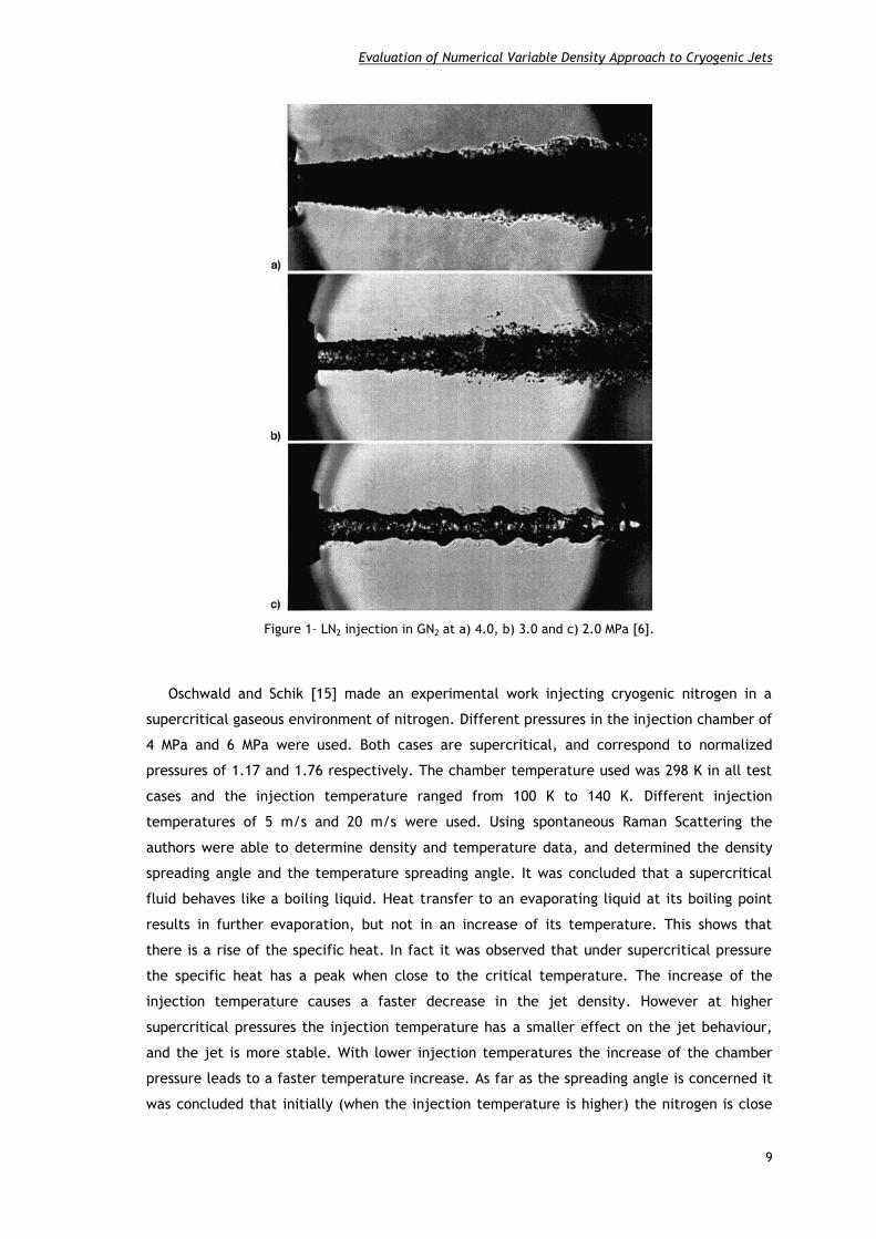
Mayer et al. [6] conducted an experimental study on the injection of cryogenic fluids in
hot fire (with combustion) and cold-flow conditions. The experiments were performed both
for single jets as for coaxial jets. In the latter case the application was the injection of fuel
and oxidizer on rocket engines. The chamber pressure employed for this study range from 1
MPa to 10 MPa. For the hot fire conditions only coaxial jets of gaseous hydrogen and liquid
oxygen (LOX) were used. At these conditions, when ignited, the flow shows no droplets which

Eduardo Luís Santos Farias Antunes
8
is attributed to rapid vaporization and to the decrease of aerodynamic forces between the
LOX and the H2 due to the reduction of density in the 3500K hot reaction zone. It was
expected that a decreased H2 injection temperature would lead to an increase of H2 density
that would intensify the mixing process. However, it was found that increasing chamber
pressure has a greater effect in intensified the mixing process, due to an increase in H2
density, than a decrease in H2 injection temperature. On cold-flow conditions both coaxial
jets and singles jets were used. Liquid nitrogen was used instead of liquid oxygen, and the
gaseous hydrogen was in some cases replaced by gaseous helium. The reason for these
substitutions was to prevent combustion. The visualizations reveal that increasing the
pressure reduces surface tension, which leads to an easier breakup of the jet and a formation
of small droplets. It is also important to notice that the average diameter of formed droplets
decreases as the ambient pressure rises, because the reduced surface tension is not strong
enough to allow the existence of large droplets. A further pressure increase causes a
complete vanish of the surface tension that leads to the disappearance of droplets formation.
At Reynolds numbers exceeding 10,000 and for pressures higher than 70% of the critical
pressure, the structure of the interface was dominated by turbulence at reduced surface
tension, and did not depend on whether the pressure was supercritical or subcritical, when at
a pressure of 6 MPa, fully under supercritical conditions, mixing is more like that between a
dense and a light liquid in a turbulent shear layer and not more a liquid/gas mixing as in
subcritical conditions. Finally, it was concluded that under certain conditions, often called
transient conditions, the nature of the jet breakup process can be extremely sensitive to
small perturbations in pressure, temperature, local mixture concentrations, and initial jet
conditions, changing extremely fast from a liquid/gas behaviour to a gas/gas behaviour and
vice versa. This study only reports qualitative results. Figure 1 shows the difference of the
injection behaviour for supercritical, transcritical and subcritical conditions, evidencing the
main conclusions reached in this work.
Evaluation of Numerical Variable Density Approach to Cryogenic Jets
9
Figure 1– LN2 injection in GN2 at a) 4.0, b) 3.0 and c) 2.0 MPa [6].
Oschwald and Schik [15] made an experimental work injecting cryogenic nitrogen in a
supercritical gaseous environment of nitrogen. Different pressures in the injection chamber of
4 MPa and 6 MPa were used. Both cases are supercritical, and correspond to normalized
pressures of 1.17 and 1.76 respectively. The chamber temperature used was 298 K in all test
cases and the injection temperature ranged from 100 K to 140 K. Different injection
temperatures of 5 m/s and 20 m/s were used. Using spontaneous Raman Scattering the
authors were able to determine density and temperature data, and determined the density
spreading angle and the temperature spreading angle. It was concluded that a supercritical
fluid behaves like a boiling liquid. Heat transfer to an evaporating liquid at its boiling point
results in further evaporation, but not in an increase of its temperature. This shows that
there is a rise of the specific heat. In fact it was observed that under supercritical pressure
the specific heat has a peak when close to the critical temperature. The increase of the
injection temperature causes a faster decrease in the jet density. However at higher
supercritical pressures the injection temperature has a smaller effect on the jet behaviour,
and the jet is more stable. With lower injection temperatures the increase of the chamber
pressure leads to a faster temperature increase. As far as the spreading angle is concerned it
was concluded that initially (when the injection temperature is higher) the nitrogen is close

Eduardo Luís Santos Farias Antunes
10
to the critical temperature and the specific heat is very high, causing an initial smaller
expansion and smaller spreading angle when compared with the cases with lower injection
temperature. However, as the temperature rises, the case with a higher injection
temperature departs from the critical temperature and the specific heat decreases leading to
a higher expansion and higher spreading angle. In their work the authors also refer that in
high pressure rocket engines the role of surface tension in the jet disintegration and mixing
process is varying locally and equilibrium thermodynamics may be not adequate to describe
the phenomena.
Chehroudi et al. [1, 7] also performed experimental studies of cryogenic jet injection
under subcritical and supercritical pressures. In these studies quantitative results were
obtained by measuring the jet growth rate/angle and the spreading rate of the mixing layer.
They injected liquid N2, at a temperature between 99 K and 110 K, in gaseous N2 at an
ambient temperature of 300 K. The critical pressure of N2 is 3.39 MPa and the ambient
pressures used in the studies range from the reduced values of 0.91 to 2.71, the critical
temperature of N2 is 126.2 K. Using photography techniques, shadowgraphy and Raman
scattering they were able to reach conclusions about supercritical injection, some of them
agreeing with Mayer et al. [6]. Figure 2 reveals that when the chamber pressure is subcritical,
the jet has a classic liquid-like appearance, but as the critical conditions are achieved the jet
seems more like a gas/gas injection and the dark core of the jet appears to vanish and
becomes less distinguishable from the ambient gas. These observations are validated by a
quantitative agreement of the jet growth rate measurements with those predicted by the
theoretical equations for incompressible variable-density gaseous jets, showing this way that
besides having the appearance it has also the behaviour of a gaseous jet. Injection of liquid
N2 in gaseous N2 at supercritical ambient temperature but at sub to supercritical pressure
shows two structural transitions. One is when the intact jet with irregularly looking surface
waves transforms into a diverging jet with ligaments and many small droplets, indicative of
the second wind-induced atomization regime. The other is when the latter structure changes,
not into the full atomization, but into a (single phase) gas/gas jet appearance slightly below
the critical pressure. As pressure is increased, the jet width increases and the structure of
the shear region changes from being dominated by ligaments and droplets to being dominated
by finger-like structures, the major structural and interfacial changes occurred at Pr = 1.03.
Above this Pr, drops are no longer detected and regular finger-like entities are observed at
the interface. They concluded that the change in the morphology of the mixing layer in
supercritical conditions is evidently due to the combined effects of reductions in the surface
tension and enthalpy of vaporization as the critical pressure is exceeded because of this
transition. It was observed that at supercritical conditions the atomization regime is fully
suppressed and they suggest that at these conditions cryogenic jet can indeed be treated like
variable density gas jets as most of results obtained are similar to these ones. Finally,
Chehroudi et al. [1] concluded that at critical and supercritical conditions, small changes in

Evaluation of Numerical Variable Density Approach to Cryogenic Jets
11
temperature at fixed pressure cause wide variations of density, thermal conductivity and
mass diffusivity. This conclusion is also shared by Mayer et al. [6].
Figure 2 - Software magnified images of the jet at its outer boundary showing the transition to the gas-
jet like appearance, starting at just below the critical pressure of the injected fluid. Images are at a
fixed supercritical chamber temperature of 300 K [1].
Mayer and Telaar [16] have made one experimental work investigating the injection of
cryogenic nitrogen in a gaseous nitrogen environment and the nitrogen/helium coaxial
injection. Unlike the previous work of Mayer et al. [6] which only obtained qualitative results,
this work obtained also quantitative results by the evaluation of the jet spreading angle using
the shadowgraphy technique. For this experiment the injected nitrogen was at a temperature
of approximately 100 K and the ambient gaseous nitrogen at a temperature of 300 K. The
chamber pressure used range from 1 MPa to 6 MPa, encompassing this way both subcritical
and supercritical pressure conditions. These authors firstly studied the nitrogen properties
around the critical point. They conclude that at the critical point the densities of the gas and
the liquid phase become the same, also the fluid properties vary remarkably around the
critical point, with the specific heat experiencing a peak near this point and the surface
tension decreasing as the pressure and temperature rise approaching critical values, this
conclusion was also achieved by Chehroudi et al. [7]. The surface tension totally disappears
when both pressure and temperature are supercritical and there is no longer phase
equilibrium. However it’s important to note that even above the critical pressure, surface
tension is still present as long as the critical mixing temperature is not exceeded. The
interpretation of the images obtain by the shadowgraphy technique in the cryogenic nitrogen
injection led to the conclusion that at subcritical conditions the flow is controlled by
aerodynamic and capillary forces, showing a wavy surface and droplet detachment. As the
pressure rise in the subcritical range there are an increased number of droplets formed due to
Eduardo Luís Santos Farias Antunes
12
the decreased surface tension. At supercritical conditions shear forces exceed the capillary
forces, which eventually disappear, and the flow start to be dominated by shear forces and
the jet expansion, in fact in the trans- and supercritical regime, the surface tension plays
only an initial role when the fluid is still below the critical mixing temperature. Finally, it was
concluded that cryogenic jets in the supercritical regime, well above the critical point, show
a purely gas-like behaviour.
Another experimental work on subcritical and supercritical liquid/gas mixing was
performed by Segal and Polikhov [4]. In their work they injected a liquid into a gaseous
nitrogen environment with reduced temperatures ranging from 0.68 to 1.28 and reduced
pressures ranging from 0.2 to 2.2, the injection speed ranged from 7 m/s to 25 m/s having
the jet a Reynolds number between 11000 and 42000. The injected fluid chosen was FK-5-1-
12 [CF3CF2C(O)CF(CF3)2] for its good thermal stability, good spectroscopic properties, and the
relatively low critical point, pc =18.4 atm, Tc=441 K. It was used the technique of planar laser
induced fluorescence (PLIF) to measure the density and the density gradients. By the analysis
of the results it was concluded that surrounding gas inertia and surface tension forces
dominate the mixing process in the subcritical case, pronounced ligament formation was
observed at these conditions when the density gradient tends to be the highest. However, as
transcritical conditions are achieved it is apparent a decrease importance of surface tension
which manifests through the smoothening of the liquid-gas interface. Ligaments formation
tends to significantly decrease. The ligament shape is similar to descriptions available in
literature described before as finger-like structures or clusters. Packets of liquid continued to
detach from the injected fluid and the density-gradient value decreased. With increased
pressure and temperature above the critical conditions, the jet behaviour changed again:
density-gradient values drastically decreased and approached values characteristic for a
laminar jet at STP conditions, this type of a liquid/gas interface behaviour was described in
previous computational results referred by authors but not seen in previous experiments. At
supercritical conditions the mixing process is described as being controlled by vaporization
rate of the injected fluid. The transitional mixing is defined as a domain when both
subcritical and supercritical mixing types can be present, both droplet formation and
irregularly shaped material broke from the injected fluid. This type of mixing is observed
when only one thermodynamic variable exceeds its critical value or when either the pressure
or the temperature was slightly below the critical value, thus supercritical mixing is possible
even when only one thermodynamic variable exceeds its critical value.
It was observed in several experimental works that the processes which control the
injection mechanism in the subcritical case are different from the ones that control it in the
supercritical case. Thus it is important to find theories and computational models which can
better predict the fluid behaviour under supercritical conditions. Several experimental works

Evaluation of Numerical Variable Density Approach to Cryogenic Jets
13
suggested that under supercritical conditions the liquid jet has a gas-like behaviour, this way,
using variable density gas models to study supercritical jets is one possible approach to this
problem. The variable density effects in axisymmetric isothermal turbulent jets for sub-
critical conditions were studied by Sanders et al. [17]. These authors used the standard "k-ε"
model and the second order Reynolds stress model with first- and second-order turbulence
models to obtain velocities, dissipation rate, spreading rate, turbulence kinetic energy,
velocity decay on the centreline and unmixedness and then compare the results obtain for
both model with the experimental results obtain by other authors. The governing equation
are solved using an algorithm similar to the TEACH code. It was concluded that the influence
of varying density is not considered to be dependent on the precise value of the spreading
rate, thus there is no significant influence of density ratio on the spreading rates in both
models, as also observed in some experimental works. The influence of including buoyancy in
the calculations with a density ratio above 1 is to decrease the spreading rates. However,
without buoyancy it was observed a slower velocity decay and faster mixture fraction decay
in the far field region. Finally the authors concluded that the "k-ε" model cannot adequately
simulate the buoyancy turbulence production and, although the differences are small, the
Reynolds stress model showed better results than the "k-ε" model. This work had not the aim
of study supercritical conditions, but only the effects of variable density in turbulent jets.
A different hypothesis was formulated by Barata et al. [18]. Starting from the
experimental evidence that supercritical jets behave as gaseous jets, they used the algorithm
of Sanders et al. [17] to simulate sub- and supercritical conditions of a nitrogen jet injected
in a nitrogen ambient. In their work they simulated the experimental conditions of Chehroudi
et al. [7] with a chamber temperature of 300 K and an injection temperature ranging from
100 K to 110 K. The chamber normalized pressure was ranging from 0.91 to 2.71, thus having
both subcritical and supercritical pressure conditions, and the injection velocity was ranging
from 1.71 m/s to 3.12 m/s. The results obtained in this work were the dense core length and
thickness, velocity field and centreline velocity decay, scalar fields of density and mixture
fraction, jet growth rate and the axial variation of centreline density. These results were
then compared with theories and experimental work of other authors. It was observed that
the length and thickness of the dense core decreases as the chamber pressure increases and
approaches the values observed for a pure gaseous jet. Concerning the velocity decay along
the centreline it increases when the normalized pressure increases. Despite the
computational code was not written for the studied case, the numerical results of the
spreading angle showed a good agreement with the experimental values obtained by
Chehroudi et al. [7] and also with other theoretical works. However, when the density ratio
decreases below the transition value, some small disagreements with experimental data are
observed, since the jets approach the spray behaviour. This numerical work reached the
conclusion that gaseous numerical models can indeed be used in the simulations of jets under
supercritical conditions with a good degree of concordance.

Eduardo Luís Santos Farias Antunes
14
Zong et al. [19] performed a numerical work investigating cryogenic nitrogen injection and
mixing into supercritical gaseous nitrogen. The nitrogen injection simulation was conducted
through a circular duct with an inner diameter of 0.254 mm. The injected cryogenic nitrogen
was at a temperature of 120 K and gaseous nitrogen in the chamber was at a temperature of
300 K while the chamber pressure was ranging from 42 atm to 93 atm. The fluid was injected
at 15 m/s, as reference the critical pressure and temperature of nitrogen are 34 atm and 126
K respectively so all the tested cases are at supercritical conditions. The model used in this
work accommodates full conservation laws, real-fluid thermodynamics and transport
phenomena over the entire range of fluid states of concern. For turbulent closure was used a
large-eddy simulation technique. This work was very comprehensive in terms of obtained
results being presented the density and density gradient, specific heat, temperature,
vorticity fields, velocity, kinematic viscosity, thermal diffusivity and other variables. An
important conclusion this work was that due to the continuous variation of fluid properties
through the jet and surrounding ambient, conventional treatment of fluid jets at low
pressures in which the liquid and gas phases are solved separately and then matched at the
interfaces often leads to erroneous results. The problem becomes even more exacerbated
when the fluid approaches its critical state, around which fluid properties exhibit anomalous
sensitivities with respect to local temperature and pressure variations. Thus, a prerequisite of
any realistic treatment of supercritical fluid behavior lies in the establishment of a unified
property evaluation scheme valid over the entire thermodynamic regime. The authors also
claim that in the vicinity of the critical point a scaled equation of state must be used.
Concerning the numerical results obtained for the fluid properties it was observed a sharp
decrease of the density near the critical point as the temperature increases, it was also
observed that the temperature sensitivity of the specific heat depends strongly on pressure.
It increases rapidly as the fluid state approaches the critical point, and theoretically becomes
infinite exactly at the critical point, this observation was also made in some experimental
studies described before [15, 16]. However, at very supercritical conditions (9.4 MPa) the
fluid shows a change in its behavior, the specific heat displays a very small variation through
the critical temperature and the density shows a smooth transition as the temperature
increases. The results obtained for the jet injection behaviour show the appearance of large-
scales instability waves near the injector in higher ambient pressures, also thread-like
entities emerge from the jet surface at these pressures (9.4 MPa). It was also seen that high
ambient pressures facilitate the entrainment of ambient gaseous nitrogen into the cold jet
fluid which increases the mixing process. Other reason for the increase of the mixing process
in high ambient pressure is the decreasing of the density stratification at these pressures, the
density stratification is responsible for inhibit of the formation of instability waves which
accelerate the mixing process.
Sierra-Palares et al. [20] made a numerical investigation with the propose of assess
turbulence models and discern which is the most suitable to use when dealing with
supercritical fluids. Unlike the majority of the studies of this subject this work had not as

Evaluation of Numerical Variable Density Approach to Cryogenic Jets
15
motivation combustion chamber applications but the application in chemical reaction
chambers. In this investigation a cryogenic nitrogen jet was injected into a pressurized
reservoir of nitrogen at ambient temperature of approximately 300 K and at a pressure of 4
MPa was simulated. The cryogenic nitrogen was injected at a temperature ranging from 118 K
to 140 K and with a velocity of 5 m/s, having this way a Reynolds number ranging from 115000
to 126000. The objective of this work was to find the best model to deal with supercritical
fluids, and several different "k-ε" and "k-ω" turbulence models were used. In order to evaluate
the performance of the various models used the dimensionless density and temperature
profiles were compared between each other and with the experimental values. Also the
residence time distribution results were compared between the models used and with other
previous work. By the comparison of the overall results the authors claim that the "k-ε
realizable" model is the one that shows the better results by having a deviation of
approximately 16% from the experimental test cases while all the other models show are
clearly less approximate with deviations above 20%. Nevertheless, the authors consider that
the other "k-ε" models show also low deviations from the experimental results. The model
could predict very well the residence time distribution even without any empirical
information. However, the authors considered that because the actual turbulent models are
not prepared to deal with the special characteristics of the supercritical turbulence, more
improvements and adaptations are still needed in the model.
Another numerical work about jet injection was performed by Schimtt et al. [21]. These
authors investigated the injection of a round nitrogen jet into a reservoir with supercritical
pressure and also the injection of a coaxial hydrogen/oxygen jet with combustion. The
objective of this numerical study was to build a real gas Large-Eddy Simulation solver that can
compute large configurations with intricate geometries. Thus an unstructured explicit solver
AVBP (which is a parallel CFD code that solves the three-dimensional compressible Navier-
Stokes on unstructured and hybrid grids) was used to compute the compressible Navier–Stokes
equations for a multispecies gas. The variables obtained in this work were the density and
density field, the temperature and the OH mass fraction field, this last only for the
investigation of the hydrogen/oxygen injection. In this work the authors describe the pseudo-
boiling temperature as the temperature at which, for a given pressure, the heat capacity at
constant pressure reaches its maximum. Two cases with different injections temperatures
were tested for the investigation of the nitrogen injection: the first case at a temperature
slightly below the pseudo-boiling temperature while the second case was at a temperature
slightly higher than the pseudo-boiling temperature. The pseudo-boiling temperature for this
investigation was 129.5 K at a reservoir pressure of 39.7 bar. The injection temperature was
126.9 K for the first case and 137 K for the second case. One of the first conclusions achieved
in this study was that at the pseudo-boiling temperature the specific heat experience a peak,
this conclusion is also shared with previous experimental and numerical studies [15, 16, 19].
It was observed that in the vicinity of the critical temperature there is a strong dependence
of the injection temperature, small changes in temperature cause big behaviour variations

Eduardo Luís Santos Farias Antunes
16
and this sensitivity to the temperature was also referred by other authors. The results for the
flow visualisation showed that when the temperature is slightly below the pseudo-boiling
temperature the jet shows ligament structures. However, for the second case of study, with
the injection temperature only 10 K higher, the jet behaviour is completely different. The
length of the dense core in the higher temperature case is smaller than in the case with lower
injection temperature and jet growth angle is higher for the high injection temperature.
Finally, it was concluded that the numerical results agree well with experimental data when
the temperature is slightly below the pseudo-boiling temperature. Nevertheless, with a
temperature slightly higher than pseudo-boiling temperature the numerical and experimental
data show discrepancies.
Recently, Kim et al. [22] performed a numerical work about supercritical nitrogen
injection. These researchers simulate the injection of liquid nitrogen with a temperature
ranging from 128.7 K to 137.0 K in a chamber at a temperature of 278 K and a pressure
ranging from 4.0 MPa to 5.98 MPa. The supercritical mixing processes were simulated by
Large-Eddy Simulation based real-fluid models, the turbulence is generated by a "k-ε"
turbulence model and were used modified CHEMKIN packages. For this work were adopted a
modified "Soave Redlich Kwong" (SRK) equation of state and a "Peng–Robinson" (PR) equation
of state, both these equation were compared between each other and also with a model using
an ideal-gas equation of state having as reference the experimental data achieved in previous
works. The Reynolds number for this work ranged from 160 000 to 200 000 and the injector
diameter was 2.2 mm. Density, temperature, turbulent viscosity, turbulent kinetic energy,
normalized axial velocity and specific heat were the obtain results used to establish the
comparison between the models and the experimental result. By the analysis of the numerical
results for the fluid properties, it was concluded that concerning the density the PR equation
shows a better agreement with the NIST data in the higher pressure case, also in the cases
with lower pressures and relatively low injection temperature the PR equation shows better
agreement. The SRK equation shows a better agreement only in the case with lower pressure
and relatively high injection temperature. Concerning the constant-pressure specific heat
both equations of state agree well with NIST data for all temperature ranges except for a
temperature of 129.5 K at near critical pressure. For the injection numerical results in the
case with higher pressure the ideal-gas model erroneously underestimates the density level in
the cold near-injector core region while the PR equation model slightly overestimate the
density level in the same region, the SRK model is the more accurate, however for axial
positions more downstream the PR equation starts to show a better agreement with the
experimental data. In the case with lower chamber pressure and relatively lower temperature
the PR equation has a better agreement with experimental data in both studied axial
positions. For the case with relatively lower pressure but higher temperature the SRK
equation shows a better agreement than PR equation. Finally, and agreeing with several other
work it was conclude that near the critical pressure the fluid properties are very sensitive to
small temperature variations it was also seen that when the pressure is equal to the critical
Evaluation of Numerical Variable Density Approach to Cryogenic Jets
17
value, there is a temperature where the constant-pressure specific heat becomes infinite,
this temperature is called the as the pseudo-boiling temperature. If the pressure is slightly
different from the critical value the pseudo-boiling temperature does not correspond to an
infinite value of the constant-pressure specific heat but only to a maximum. At supercritical
conditions, at the pseudo-boiling temperature, heat transfer to the nitrogen does not
increase its temperature but merely increases its specific volume. It was also concluded that
an increase in the pseudo-boiling strength might result in an increase of the cold core length.
In the present investigation, the work of Barata et al. [18] is extended to lower density
ratios, corresponding to subcritical pressures, and the limits of application of the variable
density approach to supercritical jets is investigated.

Eduardo Luís Santos Farias Antunes
18

Evaluation of Numerical Variable Density Approach to Cryogenic Jets
19
Chapter 2
Mathematical Model
2.1 Governing Equations
The method to solve variable density jet flows is based on the solution of the conservation
equations for momentum and mass. Turbulence is modeled with the “k~” turbulence model.
A similar method has been used for three-dimensional or axisymmetric flows and only the
main features are summarized here.
In the conservation equations, mass weighted averaging is applied to avoid the
appearance of many terms involving density fluctuations for which additional models are
needed. A mass averaged quantity is defined as
~
. (3)
For the governing equations the standard parabolic truncation is employed. The mass
averaged partial differential equations governing the steady, variable density axisymmetric
flow may be written in cylindrical polar coordinates as
r
vur
rx
p
r
UVr
rx
UU
''11~
(4)
r
ww
r
vvr
rx
p
r
VVr
rx
UV ''''11~~
(5)
and the continuity equation as
01
r
Vr
rx
U (6)
To describe mixing of gases, the mixture fraction F, that represents the mass fraction
of the nozzle fluid, is introduced. It obeys a convection-diffusion equation of the form

Eduardo Luís Santos Farias Antunes
20
r
fvr
rr
VFr
rx
UF
''11~
(7)
In “k~” turbulence model, the Reynolds stresses are expressed in terms of the local
strain rate:
j
j
tij
i
j
j
it
x
uk
x
u
x
uj
ui
u~
3
2~~
''~
(8)
with
2kCt (9)
The scalar flux in equation (7) is approximated with a gradient transport assumption
if
t
x
Ff
iu
''
~
(10)
From the foregoing we can deduced the parabolized set of equations in cylindrical
coordinates where the generalized equation is
S
drDr
rrr
rrU
x
~
1~1~ (11)
where ~
may stand for any of the velocities, turbulent kinetic energy, dissipation, or scalar
property, and S take on different values for each particular ~
, described in detail by
Sanders et al [17].
The mean density can be obtained from the mean mixture fraction using the equation
state. With constant pressure this leads to
FF
o
11 (12)
where density fluctuations have been neglected. This is allowed in isothermal jets because
the instantaneous density, for which equation (12) is exact, is approximately a linear function
of the instantaneous mixture fraction [18].

Evaluation of Numerical Variable Density Approach to Cryogenic Jets
21
2.2 Numerical Method
The governing equations are solved using a parabolized marching algorithm which
resembles the (elliptic) TEACH code [17]. The computations are performed by using the
continuity equation to obtain the radial velocity (V). Using the radial momentum equation for
V and solving a pressure correction equation for V in radial direction did not show any
difference with the use of the continuity equation [17]. In this approach the numerical model
was applied to variable density jets and for the present case it was used for the study of
liquid cryogenic jets under
In order to determine the tangent of the jet spreading angle is used the Half Width of Half
Maximum of the Velocity (HWHMV), this routine has the function of determine the radial
distance from the centerline (r) at which the axial mean velocity (U) is half of the maximum
velocity localized in the centerline. This routine analysis all the points in the radial direction
comparing them with half of the centerline velocity, when the routine finds a point bellow
this value it saves the point before that.
2.3 Boundary Conditions
There are four boundaries in the computational domain, in these boundaries dependent
variables are specified: an inlet and outlet plane, a symmetry axis and a free boundary
parallel to the axis. The sensitivity of the solutions to the locations of the boundaries was
investigated in previous works, and their final position is sufficiently far away from the jet so
that the influence on the computed results is negligible [18]. At the inlet boundary the 1/7th
power law turbulent velocity profile, represented in equation (13), was used for the axial
velocity at the jet exit.
The radial velocity is zero at the jet exit and in ambient. The mixture fraction is one at
the jet exit and zero in the ambient. On the symmetry axis, the normal velocity vanishes, and
the normal derivatives of the other variables are zero. At the outflow boundary, the gradients
of dependent variables in the axial direction are set to zero.
The flow configuration can be observed in Figure 3. The injector nozzle has a diameter of
2.54×10⁻⁴ m while the domain of study has an axial length of 1.77×10⁻² m and a radial length
of 3.49×10⁻³ m. The test conditions for the present study of different densities ratios are
presented in Table 1.
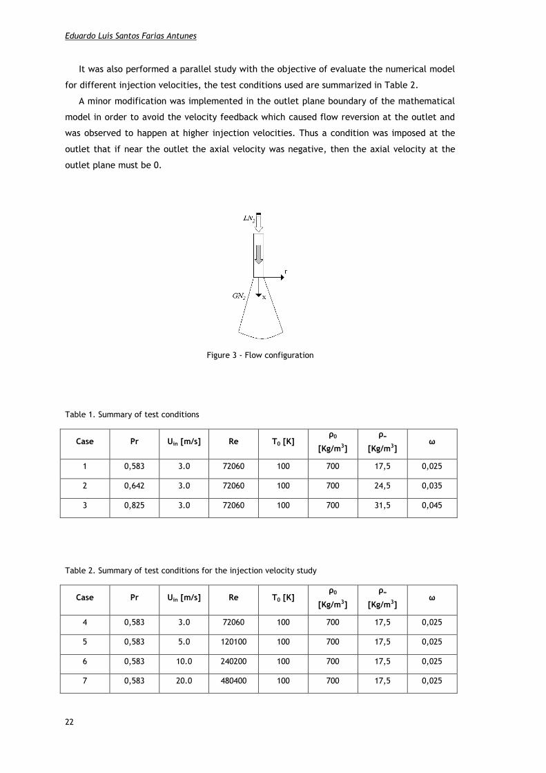
Eduardo Luís Santos Farias Antunes
22
It was also performed a parallel study with the objective of evaluate the numerical model
for different injection velocities, the test conditions used are summarized in Table 2.
A minor modification was implemented in the outlet plane boundary of the mathematical
model in order to avoid the velocity feedback which caused flow reversion at the outlet and
was observed to happen at higher injection velocities. Thus a condition was imposed at the
outlet that if near the outlet the axial velocity was negative, then the axial velocity at the
outlet plane must be 0.
Figure 3 - Flow configuration
Table 1. Summary of test conditions
Case Pr Uin [m/s] Re T0 [K] ρ0
[Kg/m3]
ρ∞
[Kg/m3] ω
1 0,583 3.0 72060 100 700 17,5 0,025
2 0,642 3.0 72060 100 700 24,5 0,035
3 0,825 3.0 72060 100 700 31,5 0,045
Table 2. Summary of test conditions for the injection velocity study
Case Pr Uin [m/s] Re T0 [K] ρ0
[Kg/m3]
ρ∞
[Kg/m3] ω
4 0,583 3.0 72060 100 700 17,5 0,025
5 0,583 5.0 120100 100 700 17,5 0,025
6 0,583 10.0 240200 100 700 17,5 0,025
7 0,583 20.0 480400 100 700 17,5 0,025

Evaluation of Numerical Variable Density Approach to Cryogenic Jets
23
Chapter 3
Results and Discussion
Introduction
In this chapter the numerical results achieved in the present work will be presented and
discussed.
The first subchapter includes the study of the influence of the ratio between the injected
fluid density and the chamber pressure density in the several variables analyzed. The study
was performed for three different density ratios, ω = 0.025, 0.035 and 0.045. For these 3 test
cases were obtained results over the Half Width of Half Maximum Velocity (HWHMV) which
was used to perform the calculation of the jet spreading angle. Results are shown about the
axial variation of the centerline density and the centerline velocity decay for each studied
case. In this chapter, the velocity field and the scalar fields of density and mixture fraction
also presented and analyzed for all three cases. The results of the axial variation of the
centerline density, centerline velocity decay and the half width of half maximum velocity are
then compared between each other by the presentation, for each variable, of a graphic
including the three studied cases. The results of the centerline density decay rate as well as
the results of the centerline velocity decay rate are shown in a single graphic as a function to
the density ratio.
Finally, the jet spreading angle results are condensed in a single graphic as a function of
the density ratio, together with several other theoretical, experimental and numerical
results. In this graphic is also shown the limit of application of the variable density approach.
The second subchapter presents the study of the influence of the injection velocity in the
results achieved by the numerical model. In this study four different injection velocities, Uin =
3, 5, 10 and 20 m.s-1, were used with a density ratio of ω = 0.025. The axial variation of the
centerline density, centerline velocity decay and half width of half maximum velocity were
obtain for the four cases and compared between each other. Also the velocity and scalar
fields of mixture fraction and are shown for the cases 5, 6 and 7 of Table 2 in this subchapter
with the purpose of visualize the jet structure. The objective of this second part of the work
was not to compare the obtained results with previous works, but instead to get a better
understanding of the behavior of the numerical model.

Eduardo Luís Santos Farias Antunes
24
3.1 Study of the density ratio influence
The study of the density ratio influence in the injection behavior is the main objective of
the present work.
Barata et al.18 performed an initial investigation aimed to evaluate the capabilities of a
computational method developed for incompressible but variable density flows when applied
to supercritical conditions. Their results have shown a good agreement with the experimental
data, but they only considered intermediate density ratios from 0.05 to 0.14. The present
work extends the investigation of Ref. 18 to much lower density ratios and investigates the
limits of application of the variable density approach to supercritical jets. For this objective
the same computational model is used in sub-near critical conditions that are beyond the
conditions for which the computational model was initially developed. In the present
investigation several different density ratios were tested in order to define the limits of
applicability of the numerical model. After the limit of applicability of the variable density
model has been found, three different conditions were studied in detail within the range of
applicability. The results achieved for these three conditions are shown in the present
subchapter. The conditions outside the limit of applicability of the variable density model
were not subjected to further studies, since it was verified that the numerical model does not
work properly at those conditions.
Figures 4, 5 and 6 show the graphics of the velocity, mixture fraction and density fields for
the density ratios of ω = 0.025, 0.030 and 0.045 respectively. In these graphics the horizontal
axis represents the axial distance to the injector (X) while the vertical axis represents the
radial distance to the centerline of the jet flow (r). In the graphics of the velocity field, the
velocity is represented by a vector for each point of the domain where the length of the
vector represents the magnitude of the velocity. The mixture fraction and density scalar
fields are represented by colored contours and with a color legend to allow the identification
of the mixture fraction and density values in the graphic. The mixture fraction is zero when
all fluid is chamber fluid and has the value 1 when is injected fluid. These graphics allow the
visualization of the main structure of the jet.
Figures 7, 8 and 9 show the axial variation of the centerline density for the density ratios
of ω = 0.025, 0.030 and 0.045 respectively. The horizontal axis represents the axial distance
to the injector, normalized by the injector diameter, while the vertical axis represents the
density expressed in kg.m-3. These graphics allow the determination of the dense core length
and this way helping to know the jet penetration. The Figure 10 shows the same results of
Figures 7 to 9 but in the same graphic and in a logarithmic scale to facilitate the comparison
between each other.
Figures 11, 12 and 13 show the centerline velocity decay for the density ratios of ω =
0.025, 0.030 and 0.045 respectively. The horizontal axis represents the axial distance to the
injector, normalized by the injector diameter, while the vertical axis represents axial velocity
at the injector divided by the centerline axial velocity. These graphics, like the axial

Evaluation of Numerical Variable Density Approach to Cryogenic Jets
25
variation of the centerline density, is useful to determinate the jet penetration. The three
obtained results are presented in the same graphic to allow the comparison between each
other in the Figure 14.
The Half Width of Half Maximum Velocity (HWHMV) is shown in Figures 15, 16 and 17 for
the density ratios of ω = 0.025, 0.030 and 0.045 respectively. In these graphics the horizontal
axis represents the axial distance to the injector while the vertical axis represents the radial
distance to the centerline normalized by the injector diameter. These graphics show the
radial distance at which the flow axial velocity is half the value of the axial velocity at the
centerline. The point at which the axial velocity has this value is interpreted, in the present
work, as the limit of the jet and is this way used to determine the jet spreading angle. To
allow a better comparison between the results of the HWHMV the results of the three density
ratios are shown in Figure 18.
Figure 19 shows the decay rate of the velocity and density in order to the chamber-to-
injectant density ratio for the three studied cases. This graphic summarizes the conclusions
also observed in graphics 7 to 14.
Finally the Figure 20 shows the tangent of the spreading angle versus the chamber-to-
injectant density ratio. This is the same graphic present by Barata et al.18 in their numerical
work but with the inclusion of the six more density ratios studied in the present work, of this
six studied density ratios only three are valid for the mathematical model and presented in
detail in this subchapter. Thus, Figure 21 shows the same results that are presented in Figure
20 but without the three non valid results and with the inclusion of the representation of the
variable density applicability limit. These graphics also allow the comparison between the
results obtained in the present work and the results obtained by other authors.
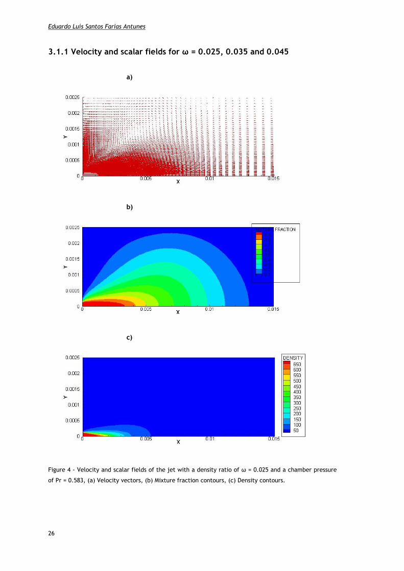
Eduardo Luís Santos Farias Antunes
26
3.1.1 Velocity and scalar fields for ω = 0.025, 0.035 and 0.045
a)
b)
c)
Figure 4 - Velocity and scalar fields of the jet with a density ratio of ω = 0.025 and a chamber pressure
of Pr = 0.583, (a) Velocity vectors, (b) Mixture fraction contours, (c) Density contours.

Evaluation of Numerical Variable Density Approach to Cryogenic Jets
27
Figure 4 shows the velocity, mixture fraction and density fields for the Case 1 described in
Table 1.
Figure 4-a) shows the velocity field within the studied domain. Close to the east boundary
and at the injector exit it is observed that the velocity obeys to the 1/7 power law turbulent
velocity profile having this way the maximum value at the centerline and then decreasing
until the injector limit. The flow velocity above the injector nozzle shows a radial component
of the velocity pointing at the centerline, this is due to the low pressures caused by the jet
flow. As the jet progress it starts to drag the surrounding fluid giving it an axial component of
the velocity. The two velocity components, imposed to the chamber fluid by the jet flow, are
called as “entrainment” and, when combined, cause the formation of a vortex with the
center localized approximately at an axial distance from the injector of X = 4.4 mm and a
radial distance from the centerline of Y = 1.4 mm. Downstream the of the center of the
vortex there is a greater divergence in the jet velocity with an increment of the radial
velocity towards the north boundary. After an axial length of approximately X = 10 mm the
radial velocity starts to decrease as the flow leaves the vortex influence zone, and at a length
of around X = 13 mm the flow has only axial velocity.
Figure 4-b) shows the mixture fraction scalar field for the domain of study. From the
injector until an axial distance of around X = 3.3 mm, close to the centerline, the mixture
fraction has a value above 0.9 indicating that there was almost no mixture of the injected
fluid with the chamber fluid. However the jet starts to mix with the chamber fluid in the
radial direction, indicating an expansion of the injected fluid. Close to the centerline, at an
axial length of approximately X = 7.2 mm, the mixture fraction reaches a value of 0.5 which
means that the injected fluid is fully mixed with the chamber fluid at this axial length.
The Figure 4-c) shows the density scalar field for the studied domain. It is observed a fast
decrease of the density just after the injector. Close to the centerline the jet density goes
from 700 kg.m-3 to 350 kg.m-3 in just approximately X = 2.3 mm. Comparing the density
evolution with the mixture fraction evolution it is possible to conclude that while the mixture
fraction at a axial distance of X = 3.3 mm at the centerline is still 0.9, at the same length,
the density close to the centerline is just 144 kg.m-3, this is, approximately 20.6 % of the
initial density. This means that the decrease of density is not caused by the mixture of
injected fluid with chamber fluid, but instead caused by the large expansion of the injected
fluid when within the injection chamber. The dense core (or dark core [4]), which can be
defined as the jet central region of high density [4], has a very small length with just
approximately 1.5 mm, this result gives even more emphases to the rapid structural change
experimented by the jet.

Eduardo Luís Santos Farias Antunes
28
a)
b)
c)
Figure 5 - Velocity and scalar fields of the jet with a density ratio of ω = 0.035 and a chamber
pressure of Pr = 0.642, (a) Velocity vectors, (b) Mixture fraction contours, (c) Density contours.
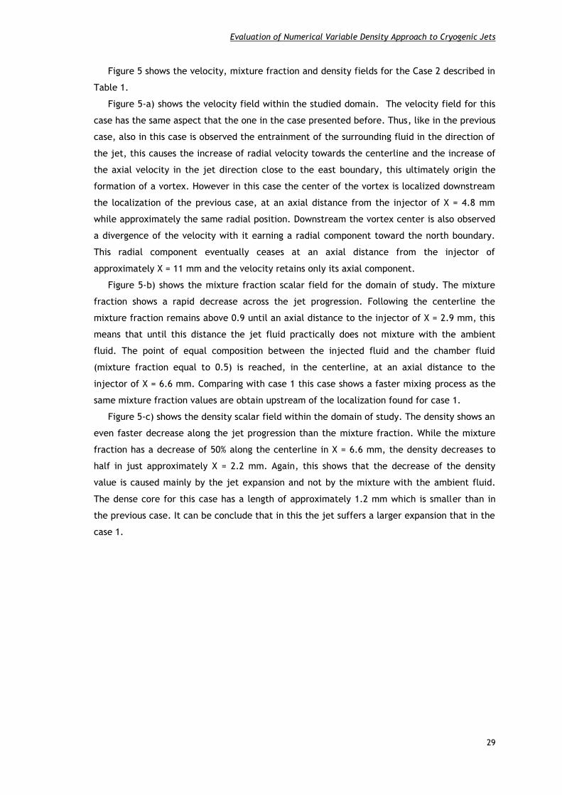
Evaluation of Numerical Variable Density Approach to Cryogenic Jets
29
Figure 5 shows the velocity, mixture fraction and density fields for the Case 2 described in
Table 1.
Figure 5-a) shows the velocity field within the studied domain. The velocity field for this
case has the same aspect that the one in the case presented before. Thus, like in the previous
case, also in this case is observed the entrainment of the surrounding fluid in the direction of
the jet, this causes the increase of radial velocity towards the centerline and the increase of
the axial velocity in the jet direction close to the east boundary, this ultimately origin the
formation of a vortex. However in this case the center of the vortex is localized downstream
the localization of the previous case, at an axial distance from the injector of X = 4.8 mm
while approximately the same radial position. Downstream the vortex center is also observed
a divergence of the velocity with it earning a radial component toward the north boundary.
This radial component eventually ceases at an axial distance from the injector of
approximately X = 11 mm and the velocity retains only its axial component.
Figure 5-b) shows the mixture fraction scalar field for the domain of study. The mixture
fraction shows a rapid decrease across the jet progression. Following the centerline the
mixture fraction remains above 0.9 until an axial distance to the injector of X = 2.9 mm, this
means that until this distance the jet fluid practically does not mixture with the ambient
fluid. The point of equal composition between the injected fluid and the chamber fluid
(mixture fraction equal to 0.5) is reached, in the centerline, at an axial distance to the
injector of X = 6.6 mm. Comparing with case 1 this case shows a faster mixing process as the
same mixture fraction values are obtain upstream of the localization found for case 1.
Figure 5-c) shows the density scalar field within the domain of study. The density shows an
even faster decrease along the jet progression than the mixture fraction. While the mixture
fraction has a decrease of 50% along the centerline in X = 6.6 mm, the density decreases to
half in just approximately X = 2.2 mm. Again, this shows that the decrease of the density
value is caused mainly by the jet expansion and not by the mixture with the ambient fluid.
The dense core for this case has a length of approximately 1.2 mm which is smaller than in
the previous case. It can be conclude that in this the jet suffers a larger expansion that in the
case 1.

Eduardo Luís Santos Farias Antunes
30
a)
b)
c)
Figure 6 - Velocity and scalar fields of the jet with a density ratio of ω = 0.045 and a chamber
pressure of Pr = 0.825, (a) Velocity vectors, (b) Mixture fraction contours, (c) Density contours.

Evaluation of Numerical Variable Density Approach to Cryogenic Jets
31
Figure 6 shows the velocity, mixture fraction and density fields for the Case 3 described in
Table 1.
Figure 6-a) represents the velocity field within the studied domain. It is observed like in
other cases that the ambient fluid next to the east wall and above the injector gains a radial
component of velocity towards the jet centerline (“entrainment” phenomena). The
surrounding fluid is also entrained in the direction of the jet and a vortex appears with its
center at an axial distance from the injector of X = 4.8 mm and a radial distance from the
centerline of Y = 1.4 mm, approximately the same position that it was on case 2. The jet
velocity then gains a radial component towards the north wall after the center of the vortex.
This radial component of the velocity starts to decrease at an axial distance of approximately
X = 8 mm and eventually becomes close to zero at an axial distance of approximately X = 11
mm.
The Figure 6-b) shows the mixture fraction scalar field for the domain of study. The jet
mixture fraction shows a rapid decrease along the centerline. In this case the jet remains
almost unmixed (with a mixture fraction value above 0.9) until an axial distance of X = 2.6
mm and then it starts to mix with the ambient fluid reaching a 0.5 mixture fraction on the
centerline at an axial distance of approximately X = 6.1 mm. In the centerline, at an axial
distance to the injector of approximately X = 12.7 mm, the mixture fraction is below 0.1
indicating that after this point injected fluid is fully dispersed into the ambient fluid,
comparing this with the velocity field at the same distance, can be stated that the jet does
not exist anymore after this point. Comparing with the previous cases, it is possible to
conclude that for this case the mixture fraction decreases faster than in previous studied
cases with lower chamber pressures.
Figure 6-c) shows the density scalar field within the domain of study. The jet shows a very
fast decrease of the density along the centerline with the value of the density in the
centerline decreasing by half in less than 2.2 mm from the injector. When compared with the
mixture fraction which is half of its initial value at an axial distance from the injector of X =
6.1 mm, this show that the density decrease of the jet fluid is not caused by the mixing of the
jet fluid with the less dense ambient fluid, because at the point that the density is half the
initial density the mixture fraction is still above 0.9 indicating that almost no mixing with the
ambient fluid has already happen at this point. So the decrease in density must be caused by
the rapid expansion of the jet fluid as it enters in the injection chamber. The jet dense core
in this case has a length in the centerline of approximately 1.2 mm.
Comparing the velocity and scalar fields for the three studied cases it is possible to
conclude that in general the jet behavior is very similar between each other. This was
expected because all the test cases are in the subcritical range with just only slightly
increments of pressure from case to case. However, some differences can be noted between
the test cases, for example in the velocity field is observed that at an axial length of X = 15
mm the flow has a greater velocity for the case with lower pressure and density ratio (case 1)
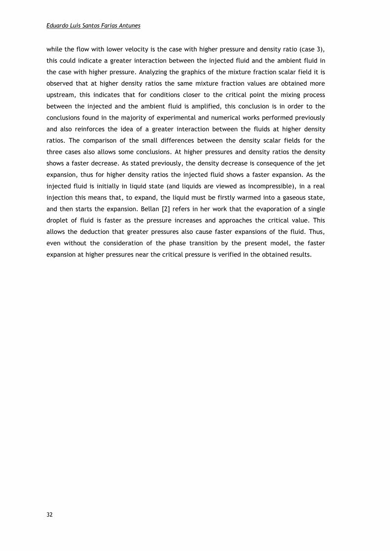
Eduardo Luís Santos Farias Antunes
32
while the flow with lower velocity is the case with higher pressure and density ratio (case 3),
this could indicate a greater interaction between the injected fluid and the ambient fluid in
the case with higher pressure. Analyzing the graphics of the mixture fraction scalar field it is
observed that at higher density ratios the same mixture fraction values are obtained more
upstream, this indicates that for conditions closer to the critical point the mixing process
between the injected and the ambient fluid is amplified, this conclusion is in order to the
conclusions found in the majority of experimental and numerical works performed previously
and also reinforces the idea of a greater interaction between the fluids at higher density
ratios. The comparison of the small differences between the density scalar fields for the
three cases also allows some conclusions. At higher pressures and density ratios the density
shows a faster decrease. As stated previously, the density decrease is consequence of the jet
expansion, thus for higher density ratios the injected fluid shows a faster expansion. As the
injected fluid is initially in liquid state (and liquids are viewed as incompressible), in a real
injection this means that, to expand, the liquid must be firstly warmed into a gaseous state,
and then starts the expansion. Bellan [2] refers in her work that the evaporation of a single
droplet of fluid is faster as the pressure increases and approaches the critical value. This
allows the deduction that greater pressures also cause faster expansions of the fluid. Thus,
even without the consideration of the phase transition by the present model, the faster
expansion at higher pressures near the critical pressure is verified in the obtained results.

Evaluation of Numerical Variable Density Approach to Cryogenic Jets
33
3.1.2 Axial variation of centerline density for ω = 0.025, 0.035 and 0.045
The Figure 7 shows the axial variation of the centreline density for the Case 1 described in
Table 1.
Figure 7 - Axial variation of the centerline density with a density ratio of ω = 0.025 and a chamber
pressure of Pr = 0.583.
The density remains approximately its initial value of ρ = 700 kg.m-3 until an axial distance
of X/D = 3 diameters, which corresponds to the potential core. After this point, the density
starts an accentuated decrease which corresponds to the jet rapid expansion. The density
decrease starts to slows down at an axial distance of X/D = 15 diameters, at this point the
centerline density has a value of approximately ρ = 100 kg.m-3. After this point the centerline
density decreases at a slower rate, reaching a value of around ρ = 20 kg.m-3 at an axial
distance of X/D = 50 diameters. Comparing this graphic with Figure 4-c) it is possible to see
that the start of the accentuated decrease of the centerline density is close to the point at
which the jet dense core disappears.
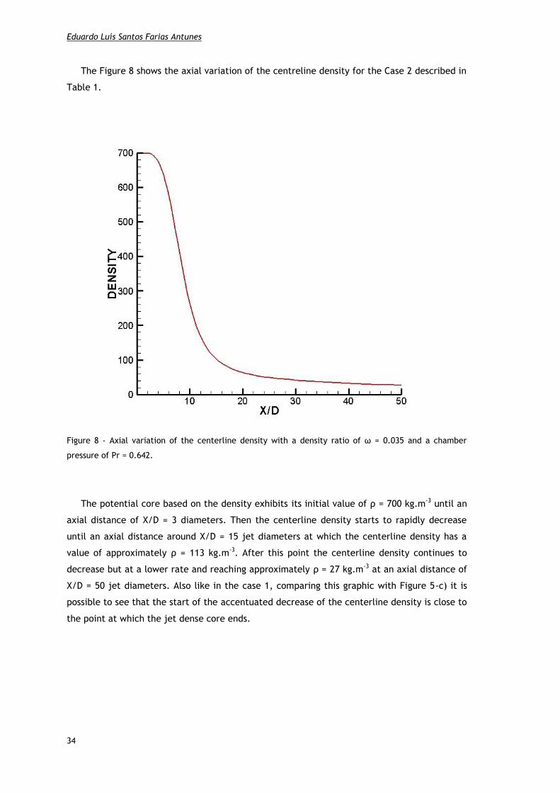
Eduardo Luís Santos Farias Antunes
34
The Figure 8 shows the axial variation of the centreline density for the Case 2 described in
Table 1.
Figure 8 - Axial variation of the centerline density with a density ratio of ω = 0.035 and a chamber
pressure of Pr = 0.642.
The potential core based on the density exhibits its initial value of ρ = 700 kg.m-3 until an
axial distance of X/D = 3 diameters. Then the centerline density starts to rapidly decrease
until an axial distance around X/D = 15 jet diameters at which the centerline density has a
value of approximately ρ = 113 kg.m-3. After this point the centerline density continues to
decrease but at a lower rate and reaching approximately ρ = 27 kg.m-3 at an axial distance of
X/D = 50 jet diameters. Also like in the case 1, comparing this graphic with Figure 5-c) it is
possible to see that the start of the accentuated decrease of the centerline density is close to
the point at which the jet dense core ends.

Evaluation of Numerical Variable Density Approach to Cryogenic Jets
35
The Figure 9 shows the axial variation of the centreline density for the Case 3 described in
Table 1.
Figure 9 - Axial variation of the centerline density with a density ratio of ω = 0.045 and a chamber
pressure of Pr = 0.825.
Observing the graphic it is concluded that it is very similar to the graphics for cases 1 and
2. The centerline density for this case also remains approximately at its initial value of ρ =
700 kg.m-3 until approximately an axial distance of X/D = 3 diameters, again corresponding to
the potential core size. Then it undergoes into an accentuated decrease, which corresponds
to the jet rapid expansion, until approximately an axial length of X/D = 15 diameters at which
the centerline density has approximately the value of ρ = 108 kg.m-3. After this, the
centerline density continues to decrease, at a lower rate, reaching a value of approximately ρ
= 35 kg.m-3 at X/D = 50 jet diameters of axial distance. Again, comparing this graphic with
Figure 6-c) it is possible to see that the start of the accentuated decrease of the centerline
density is close to the point at which the jet dense core disappears.
There are no big differences between the axial variation of the centerline density for the
three studied cases, with the graphics being very similar for all, and revealing a potential
core size of 3 diameters. However, looking to Figure 10, which represent the results shown

Eduardo Luís Santos Farias Antunes
36
above, in the same graphic and in a logarithmic scale, is possible to notice some small
differences and take some conclusions from them. The accentuated decrease of the
centerline density starts at the same axial length for all the studied cases. However, in the
cases with higher chamber pressure and density ratio the decrease happens at a slightly
higher rate, indicating this way a faster expansion despite the pressure gradient, between the
injection pressure and the chamber pressure, is lower in these cases. As the ambient fluid
density is higher in the cases with higher pressure, after the jet expansion, the density
decrease rate slows down faster for the cases with higher chamber pressure and the final jet
centerline density is higher for these cases. A final conclusion is that the length and thickness
of the dense core slightly decrease as the chamber pressure increases, this conclusion was
also achieved by the analysis of Figures 4-c), 5-c) and 6-c) in the last section.
Figure 10 - Axial variation of the centerline density in a logarithmic scale for the cases 1, 2 and 3.

Evaluation of Numerical Variable Density Approach to Cryogenic Jets
37
3.1.3 Centerline velocity decay for ω = 0.025, 0.035 and 0.045
The Figure 11 shows the centerline velocity decay for the case 1 described in Table 1.
Figure 11 - Centerline velocity decay for a density ratio of ω = 0.025 and a chamber pressure of Pr =
0.583.
This graphic show, at each point, how many times the centerline velocity has decreased
from its initial injection value. Analyzing the graphic it can be seen that the centerline
velocity slightly decreases until an axial length of approximately X/D = 15 injector diameters
at which the velocity is 1.27 times lower than the initial velocity. After this axial length the
velocity decay rate starts to rise and the velocity experiences a faster decrease, at this stage
the velocity decay is almost linear with a rate of α = 0.35280. Comparing with Figure 4-a), it
is possible to see that this increase of the centerline velocity decay correspond approximately
to the axial localization of the center of the vortex. This suggests that the vortex can be
responsible for the dissipation of a large part of the jet energy. The centerline velocity
decreases by half in an axial length of approximately X/D = 24 injector diameters. The rate of
the centerline velocity decay starts to slow down at a length of 45 diameters and at X/D = 50
diameters the centerline velocity has decayed approximately 7.9 times.

Eduardo Luís Santos Farias Antunes
38
By the analysis of the present graphic it is possible to determine the potential core size
based on the velocity decay. In this investigation it is considered the existence of the
potential core until a velocity decay of 10%, thus it was conclude that the potential core
based on the centerline velocity decay has a size of X/D = 8.30 diameters.
The Figure 12 shows the centerline velocity decay for the case 2 described in Table 1.
Figure 12 Centerline velocity decay for a density ratio of ω = 0.035 and a chamber pressure of Pr =
0.642.
By the analysis of the graphic it is observed that, like in the previous case, the centerline
velocity decay initially rises at a slow rate and then, after a length of approximately X/D = 15
diameters, at which the velocity has decayed 1.35 times, the rate of the centerline velocity
decay starts to rise. Again the bigger rise of the velocity decay’s rate is verified close to the
distance at which, in Figure 5-a), is seen the center of the vortex. At this stage, the velocity
decay is almost linear with a decay’s rate of α = 0.48244. The centerline velocity has half the
value of the initial velocity at an axial distance of approximately X/D = 22.5 injector
diameters. The rate of velocity decay starts to decrease at around X/D = 46 diameters and at
a length of X/D = 50 diameters the centerline velocity has decayed approximately 10.7 times.
The 10% decay of the centerline velocity is achieved after an axial length of approximately
X/D = 7.84 diameters which corresponds to the potential core size.
Evaluation of Numerical Variable Density Approach to Cryogenic Jets
39
The Figure 13 shows the centerline velocity decay for the case 3 described in Table 1.
Figure 13 Centerline velocity decay for a density ratio of ω = 0.045 and a chamber pressure of Pr =
0.825.
Observing the graphic can be seen that the centerline velocity slightly decreases until an
axial length of approximately X/D = 15 injector diameters at which the velocity is 1.43 times
lower than the initial velocity. Then, like in previously analyzed cases, the centerline velocity
decay rate starts to rise and the velocity experiences a faster decrease, also in this case the
greater variation in the centerline velocity decay rate is observed at the same length of the
center of the vortex seen on Figure 6-a). The centerline velocity decay has the value equal to
2, which corresponds to a decrease in the centerline velocity by half, at an axial distance of
approximately X/D = 21.6 diameters. The centerline velocity decay continues to rise at a fast,
almost constant, rate of α = 0.62668, until an axial distance of 48 diameters. Finally at a
length of X/D = 50 diameters the centerline velocity has decayed approximately 13.3 times.
The potential core based on the centerline velocity decay has a length of approximately
X/D = 7.47 diameters.

Eduardo Luís Santos Farias Antunes
40
The kind of evolution of the centerline velocity decay is very similar for the three studied
cases, as described above. However at higher density ratios is observed a greater increase of
the centerline velocity decay than for lower density ratios. As can be observed in Figure 14,
which combines the three results presented above in a single graphic for an easier comparison
between each other, the velocity decay is almost equal for the three cases until an axial
distance of approximately X/D = 10 diameters. Then the higher pressure cases starts to have a
slightly higher increase which, as the axial distance to the injector increases, becomes a
bigger difference. These results complement the conclusions achieved in the join analysis of
the Figures 4-a), 5-a) and 6-a) that at higher chamber pressures the jet experiences a major
loss of velocity and indicates that the greater loss of velocity happens as the jet passes at the
same length of the vortex center, suggesting this way that a great part of the kinetic energy
loss by the jet is dissipated by the formed vortex.
One interesting result is the potential core sized based on the centerline velocity decay
which is different to the density based potential core size obtained previously. The density
based potential core has almost the same size of X/D = 3 diameters for the three test cases,
however, when based in the centerline velocity decay the potential core has a bigger size and
is different for the three test cases. It is also observed that the potential core size based on
the centerline velocity decay slightly decreases as the density ratio increases. These results
are different from the ones obtained for the one-phase flow where usually the potential core
based on the centerline density and on the centerline velocity decay have approximately the
same value.
The difference between the potential core based on the centerline density and the one
based on the centerline velocity decay together with the evidences of the jet expansion,
reached in section 3.1.1, suggest that the fluid expansion after injection may contribute with
kinetic energy to the flow reducing the centerline velocity decay, and this way increasing the
jet potential core based on the centerline velocity decay.
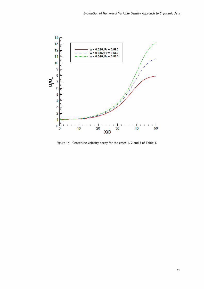
Evaluation of Numerical Variable Density Approach to Cryogenic Jets
41
Figure 14 - Centerline velocity decay for the cases 1, 2 and 3 of Table 1.

Eduardo Luís Santos Farias Antunes
42
3.1.4 Half width of half maximum of the velocity for ω = 0.025, 0.035 and
0.045
The Figure 15 shows the half width of half maximum of the velocity for the case 1
described in Table 1.
Figure 15 - Half width of half maximum of the velocity for a density ratio of ω = 0.025 and a chamber
pressure of Pr = 0.583.
The radial distance to the centerline normalized by the injector diameter, at which the
axial velocity is half of the centerline axial velocity, is represented in this graphic. The radial
distance where the axial velocity is half of the maximum is used to determinate the jet
growth. Thus, it can be observed in the graphic that the half width of half maximum of the
velocity has two different types of progression. One almost linear which lasts from the
injector until an axial length of approximately X/D = 34 injector diameters, and other non
linear after this length. The linear part of the graphic can be defined by a straight line from
which it is possible to determinate the slope. In the non linear part of the graphic, the
definition by a straight line is not so easy. For the present work the interest lies in the linear

Evaluation of Numerical Variable Density Approach to Cryogenic Jets
43
section of the graphic and its slope is calculated using two points. The points used were
P1:[X/D = 10.050, R1/2(U)/D = 1.6168] and P2:[X/D = 30.062, R1/2(U)/D = 3.8701]. Thus the
slope of the straight line which represents the tangent of the spreading angle of the jet is tan
= 0.11261.
The Figure 16 shows the half width of half maximum of the velocity for the case 2
described in Table 1.
Figure 16 - Half width of half maximum of the velocity for a density ratio of ω = 0.035 and a chamber
pressure of Pr = 0.642.
By the analysis of the graphic it is possible to indentify an almost linear evolution of the
half width of half maximum of the velocity that extends since the injector until an axial
distance of approximately X/D = 36 injector diameters and after this point until the end of
the graphic a non linear evolution. Choosing two points in the almost linear part of the
graphic, P1:[X/D = 10.050, R1/2(U)/D = 1.5206] and P2:[X/D = 30.062, R1/2(U)/D = 3.7244], it is
possible to draw a straight line with a slope of 0.11016. Again, the straight line’s slope
represents the tangent of the spreading rate of the jet. The non linear evolution of the half

Eduardo Luís Santos Farias Antunes
44
width of half maximum of the velocity is made at a bigger rate that the linear part, this is
probably caused by the lower velocity in the jet centerline at this part of the domain, this
way the half velocity of the centerline is only found at greater radial distances and eventualy,
as the jet centerline velocity decays to lower values, becomes impossible to find within the
domains of study, a point were the velocity is half of the centerline velocity. After this
distance the half width of half maximum of the velocity is no more applicable to study the jet
growth.
The Figure 17 shows the half width of half maximum of the velocity for the case 3
described in Table 1.
Figure 17 - Half width of half maximum of the velocity for a density ratio of ω = 0.045 and a chamber
pressure of Pr = 0.825.
In this graphic, like in Figures 15 and 16, there are also two different parts, one almost
linear part from which is possible to draw a straight line, and one non linear part. The almost
linear part of the graphic extends from the injector until approximately a distance of X/D =
37 injector diameters, after this the graphic enter in the non linear part. To draw the straight
line that best reflects the half width of half maximum of the velocity in the linear part were

Evaluation of Numerical Variable Density Approach to Cryogenic Jets
45
choosen to different point of the graphic, P1:[X/D = 10.050, R1/2(U)/D = 1.4598] and P2:[X/D =
30.062, R1/2(U)/D = 3.6326]. The calculated slope of the straight line is 0.10857. As said
before, the slope of the straight line represents the jet growth.
Figure 18 includes the results shown above in a single graphic to allow a better comparison
between each other. The behavior of the half width of half maximum of the velocity is very
similar for the three cases. In all of theme there are one linear and other non linear part.
However it is possible to verified that, in the almoast linear zone, the HWHMV slope slightly
decreases as the chamber pressure rises indicating that is slightly higher at lower pressures.
This result was not expected because in several investigations performed previously it was
verified that the spreading rate increased with the increase of the chamber pressure. It can
also be verified that for the three cases, the end of the linear zone approximately
corresponds, in the graphic of the centerline velocity decay, to the axial distance where the
rate of velocity decay is more accentuated. On the other hand, was concluded in the analysis
of the centerline velocity decay that the increase of its rate happened after the vortex center
and this way could be cause by the vortex existence. Thus, one possible conclusion is that the
appearance of the non linear zone of the half width of half maximum of the velocity could be
caused by the vortex existence. At the non linear zone the evolution of the HWHMV still
remains similar in the three cases but there is an amplification of the HWHMV difference
between the cases. Finally it is possible to see that in all cases the HWHMV has a bigger
increase in the non linear zone, indicating a bigger spreading rate. The graphic not shows the
domain after X/D = 50 diameters, this is because the HWHMV algorithm only functions in a
domain were a point with half the centerline velocity can be found. After an axial distance of
X/D = 50 diameters the axial velocity is shows a small variation across the radial section and
centerline velocity has experienced a high decay (Figures 11, 12, 13 and 14), this way it
becomes difficult to find, within the domain, a point with half the velocity of the centerline.
Comparing the half width of half maximum of the velocity graphics with the centerline
velocity decay it’s possible to observe that, at each case, the jet growth rate has a different
value from the centerline velocity decay rate. Also the influence of the chamber pressure
variation is different for the two variables. While for the jet growth rate obtained by the
HWHMV the pressure change has little effect, with only a slight decrease of the jet growth
rate, for the centerline velocity decay rate the increase of the chamber pressure has a
greater effect of increasing its value.

Eduardo Luís Santos Farias Antunes
46
Figure 18 - Half width of half maximum of the velocity for the cases 1, 2 and 3 of Table 1.
3.1.5 Centerline velocity and density decay rate at various chamber-to-
injectant density ratios
Figure 19 shows the decay rates of velocity and density after the potential core for the
cases of Table 1 summarizing this way some of the information already shown in figures 7 to
14. The centerline velocity decay rate is calculated using a similar method used for the
tangent of the spreading rate. For the centerline density decay were chosen two points in the
almost linear part of the graphic of the centerline density variation, the initial centerline
density was divided by density at each point and then was made the difference between the
two obtained values and divided by the axial distance between the two values. For both
velocity and density an increase in the injection chamber pressure has as result an increase of
the decay rate which is in agreement with previous works from other authors, however this
effect is more pronounced in the velocity decay. The velocity also shows for the three cases a
higher decay rate then the density although is important to remember that the density decay
starts earlier then the velocity decay due to the longer potential core obtained for the
velocity.

Evaluation of Numerical Variable Density Approach to Cryogenic Jets
47
Figure 19 – Decay rate of the centerline velocity and density.
3.1.6 Tangent of the spreading angle at various chamber-to-injectant
density ratios
Figure 20 shows the tangent of the jet spreading angle calculated by the half width of half
maximum of the velocity in order to the density ratio. In addition to the three cases studied
previously in the present subchapter the graphic contains three more cases with different
density ratios also study in the present work, but for which no detaild results are presented,
and results obtained by other authors in previous investigations including the results of Barata
et al. [18], the investigation which the present work pretends to extend. The results achieved
in the present work are represented in red while those achieved by other authors are
represented in black.
The three other cases tested in this work had density ratio values of ω = 0.010, 0.015 and
0.020. This cases were not presented in detail at the present work due to the fact that no
valid results were found for these cases, as shown in the graphic. The spreading rates for this
cases were calculed using the half width of half maximum of the velocity like in the cases
presented above but the results obtained are too low in order to be considered valid. The

Eduardo Luís Santos Farias Antunes
48
analysis of the other results obtained for these cases also shown not to be congruent with any
theorys or experimental and numerical results obtained by other authors. Thus these results
were simply ignored in the detailed analysis presented previously for the cases 1, 2 and 3 of
the present work. However, the results obtained for the density ratios of ω = 0.010, 0.015
and 0.020 were essencial to achieved an important conclusion of the present work. By the
analysis of the results obtained for the lower density ratios it is possible to conclude that the
present numerical model can not be applied for conditions at which the density ratio between
ambient fluid and the injection fluid is bellow approximately ω = 0.025.
Figure 20 - Tangent of the spreading angle versus the chamber-to-injectant density ratio.
Figure 21 also shows the tangent of the jet spreading angle in order to the density ratio
for the cases 1, 2 and 3 studied in the present work and for results of other athors. This
graphic is similar to the graphic presented by Barata et al. [18] and to the graphic of Figure
19. But instead of present the results obtained in this investigation for the lower density
ratios, like in Figure 20, it presents the limit of applicability of the variable density approach
used in the present work. As verified in Figure 20, conditions below a density ratio of ω =
0.025 can not be predited by the present numerical model, in fact, the numerical model
shown not be able to give valid results below this density ratio. Thus, it was established as a
limit of applicability of the variable density approach a minimum value of ω = 0.025. This
limit is represented in Figure 21 by the red vertical line with a black arrow on the rigth.

Evaluation of Numerical Variable Density Approach to Cryogenic Jets
49
The three studied cases are represented in red at the graphic while the results of other
author are again represeted in black. It is possible to verified that the results obtain are very
close to the experimental results of Chehroudi et al. and also with the modelling of the same
authors. However some discrepancies are observed when comparing with results from other
authors. While all the other authores have results that show an increase the divergence angle
as the density ratio increases, in the present work that does not happens, in fact, the
divergence angle shows a sligth decrease as the density ratio increases.
Figure 21 - Tangent of the spreading angle versus the chamber-to-injectant density ratio and
representation if limit of applicability of the Variable Density approach.

Eduardo Luís Santos Farias Antunes
50
3.2 Study of the injection velocity influence
The study of the injection velocity (Uin) influence in the jet behavior is performed in the
present investigation with the main purpose of characterize the mathematical model. This
study has a smaller relevance in the present work and therefore it will be not treated as
extensively as the density ratio influence study presented in the previous subchapter. The
test cases analyzed in this subchapter are presented in Table 2. For this study all the cases
have the same chamber-to-injector fluid density ratio of ω = 0.025, but the injection
velocities are ranging from 3 to 20 m.s-1. It is important to refer that the case 4 of Table 2 has
exactly the same conditions that the case 1 of Table 1 and so, no more graphics and analysis
will be present for this case and it will be only compared with the other cases at the present
subchapter. For the other cases will be presented the results obtained by the mathematical
model.
In this study no comparisons will be made with theories or results obtained by other
authors as the main objective is to identify the behavior change of the mathematical model
at different injection velocities.
Figures 22, 23 and 24 show the graphics of the velocity, mixture fraction and density fields
for the injection velocities of Uin = 5, 10 and 20 m.s-1 respectively. In these graphics the
horizontal axis represents the axial distance to the injector (X) while the vertical axis
represents the radial distance to the centerline of the jet flow (r). In the graphics of the
velocity field, the velocity is represented by a vector for each point of the domain where the
length of the vector represents the magnitude of the velocity. The mixture fraction and
density scalar fields are represented by colored contours and with a color legend to allow the
identification of the mixture fraction and density values in the graphic. The mixture fraction
is zero when all fluid is chamber fluid and has the value 1 when is injected fluid. These
graphics allow the visualization of the main structure of the jet.
Figure 25 shows the axial variation of the centerline density for the four test cases of
Table 2. The horizontal axis represents the axial distance to the injector, normalized by the
injector diameter, while the vertical axis represents the density expressed in kg.m-3. These
graphics allow the determination of the dense core length and this way helping to know the
jet penetration.
Figure 26 shows the centerline velocity decay for the four test cases of Table 2. The
horizontal axis represents the axial distance to the injector, normalized by the injector
diameter, while the vertical axis represents axial velocity at the injector divided by the
centerline axial velocity. These graphics, like the axial variation of the centerline density, is
useful to determinate the jet penetration.
Finally Figure 27 shows the Half Width of Half Maximum Velocity (HWHMV) for the four
test cases of Table 2. In these graphics the horizontal axis represents the axial distance to the
injector while the vertical axis represents the radial distance to the centerline normalized by
the injector diameter. This graphic allows the determination of the jet spreading angle.
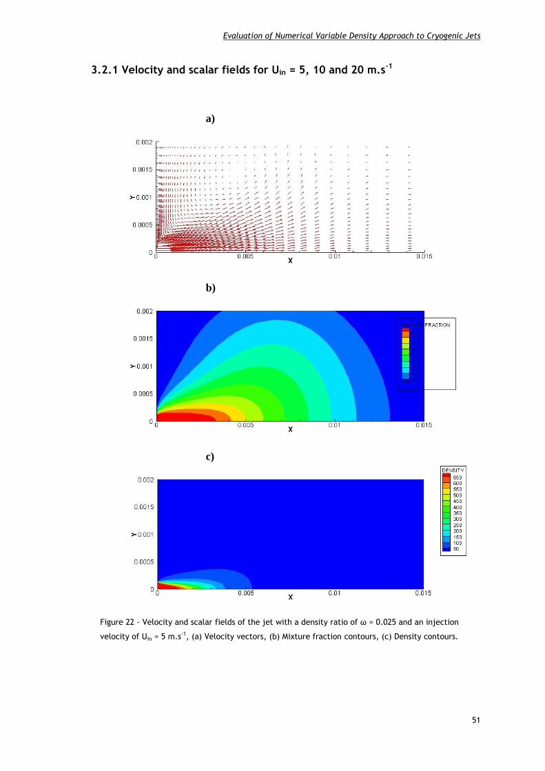
Evaluation of Numerical Variable Density Approach to Cryogenic Jets
51
3.2.1 Velocity and scalar fields for Uin = 5, 10 and 20 m.s-1
a)
b)
c)
Figure 22 - Velocity and scalar fields of the jet with a density ratio of ω = 0.025 and an injection
velocity of Uin = 5 m.s-1, (a) Velocity vectors, (b) Mixture fraction contours, (c) Density contours.

Eduardo Luís Santos Farias Antunes
52
a)
b)
c)
Figure 23 - Velocity and scalar fields of the jet with a density ratio of ω = 0.025 and an injection
velocity of Uin = 10 m.s-1, (a) Velocity vectors, (b) Mixture fraction contours, (c) Density contours.

Evaluation of Numerical Variable Density Approach to Cryogenic Jets
53
a)
b)
c)
Figure 24 - Velocity and scalar fields of the jet with a density ratio of ω = 0.025 and an injection
velocity of Uin = 20 m.s-1, (a) Velocity vectors, (b) Mixture fraction contours, (c) Density contours.

Eduardo Luís Santos Farias Antunes
54
Figures 22-a), 23-a) and 24-a) show the velocity field for the cases 5, 6 and 7 of Table 2
respectively. Comparing these graphics between each other and with Figure 4-a), case 4, can
be concluded that the velocity field for all the injection velocities have the same kind of
structure found for an injection velocity of Uin = 3 m.s-1 (case 4). Figures 22-a), 23-a) and 24-
a) show the existence of the entrainment phenomena also found in the case 4. The
appearance of a vortex above the jet flow approximately at the same location that in case 4
is visible in Figure 21-a) for the case with a injection velocity of Uin = 5 m.s-1. For the cases 6
and 7 is also observed the appearance of a vortex above the jet flow, however in these cases
the vortex has its location further downstream that in cases 4 and 5, with its center at an
axial position of approximately X = 5.8 mm and X = 6.7 mm respectively for cases 6 and 7.
The mixture fraction scalar field is shown in Figures 22-b), 23-b) and 24-b). The case with
an injection velocity of Uin = 5 m.s-1 has almost the same mixture fraction evolution obtained
for an injection velocity of Uin = 3 m.s-1. Increasing the injection velocity to Uin = 10 m.s-1 the
mixture fraction field shows a slower change of the mixture fraction value, thus pointing to a
poorer mixing process between the injected and the ambient fluid. A further increase in the
injection velocity to Uin = 20 m.s-1 causes an even poorer mixing process that the one shown in
the case with an injection velocity of Uin = 10 m.s-1, with the mixture fraction at the
centerline maintaining a value above 0.9 after an axial length of X = 5 mm.
Figures 22-c), 23-c) and 24-c) show the density scalar field for the cases 5, 6 and 7 of
Table 2 respectively. Looking to the Figure 21-c) and comparing it with Figure 4-c) is verified
that both are very similar, this way an increment of the injection velocity to Uin = 5 m.s-1 does
not have any visible influence in the jet density scalar field. The same does not happens when
the injection velocity increases to Uin = 10 m.s-1, with this injection velocity the dense core
increases and jet expansion becomes slower. A further increase in the injection velocity to Uin
= 20 m.s-1 is responsible for an even greater length of the dense core and a slower jet
expansion. These results suggest that despite the increase of the injection velocity Uin the
rate of the fluid expansion doesn’t increases in the same order and this way the injected fluid
shows a smaller interaction with the chamber fluid close to the injector.
The velocity and scalar fields are very similar for the two lower injection velocities.
However, as the injection velocity increases for values above Uin = 10 m.s-1 the velocity and
scalar field experienced some changes. So, the injection velocity must be considered as a
variable which affects the result obtained for the velocity and scalar field of density and
mixture fraction in the application of the mathematical model used in the present work.

Evaluation of Numerical Variable Density Approach to Cryogenic Jets
55
3.2.2 Axial variation of the centerline velocity for Uin = 3, 5, 10 and 20
m.s-1
Figure 25 - Axial variation of the centerline density for the cases 4, 5, 6 and 7 of the Table 2.
The Figure 25 shows the axial variation of centerline density for the studied cases. Having
the case 4 as reference, by the observation of the graphic it is possible to see that an initial
increase of the injection velocity to Uin = 5 m.s-1 causes the centerline density to decrease at
a slower rate. The case 5 also shows a longer potential core based on the density with a
length of X/D = 6.36 diameters when compared with the X/D = 5.16 diameters found in case
4, for this study the potential core based on the density is calculated by the axial distance
where the density has decayed 10%. At an axial length of around 15 diameters the density
decrease rate starts to slow down and at a length of approximately X/D = 30 diameters the
centerline density becomes almost constant until a length of X/D = 50 injector diameters
were the density has a value around 60 kg.m-3, much higher than in the other cases. In case 6
the centerline density starts to have a lower decrease rate than the case 5, however at a
length of 15 diameters continues to decrease at a higher rate that the previous case and after
an axial length of around X/D = 21 diameters the centerline density for an injection velocity
of Uin = 10 m.s-1 is lower that for Uin = 5 m.s-1. For the case 6 the potential core shows a

Eduardo Luís Santos Farias Antunes
56
length of X/D = 8.11 diameters. Finally the test case 7, with an injection velocity of Uin = 20
m.s-1, the centerline density shows a lower decrease rate than in the previous case following
a similar difference from case 6 that this case had to the case 5. It is also observable in this
case a bigger potential core than in the previous cases with a length of approximately X/D =
10.0 diameters. At an axial length of X/D = 50 diameters the value centerline density for case
7 reaches approximately the same value observed in cases 4 and 6.
Here is seen that the centerline density evolution can be highly affected by the injector
velocity, having the tendency to follows a slower evolution with the increase of the injection
velocity, so, it must be taken in consideration when the objective is to study the density
variation.
3.2.3 Centerline velocity decay for Uin = 3, 5, 10 and 20 m.s-1
Figure 26 - Centerline velocity decay for the cases 4, 5, 6 and 7 of the Table 2.
The Figure 26 shows the centerline velocity decay for the studied cases. It is observed that
the case with higher velocity decay is the one with lower injection velocity, Uin = 3 m.s-1. A

Evaluation of Numerical Variable Density Approach to Cryogenic Jets
57
small increase on the injection velocity to Uin = 5 m.s-1 causes the centerline velocity decay at
a length of X/D = 50 diameters to decrease from around 7.9 to 2.4, which represents a
decrease of approximately 70%. A further increase in the injection velocity to U in = 10 m.s-1 is
responsible for an increase in 170% of the centerline velocity decay comparatively to the case
5, reaching a value of 6.5 at an axial length of X/D = 50 injector diameters. In the case with
higher injection velocity, Uin = 20 m.s-1, the centerline velocity decay at an axial length of
X/D = 50 injector diameters reaches a value of approximately 5.1 which, compared with the
previous case corresponds to a decrease of approximately 22%.
By the analysis of the graphic it is possible to calculate the potential core based on the
velocity decay as well as the rate of the centerline velocity decay in the almost linear part
for the four studied cases. Case 5 shows a bigger potential core with a length of X/D = 9.40
diameters when compared with case 4 which has a potential core of X/D = 8.30 diameters.
This trend of an increase of the potential core with the increase of the injection velocity
happen in both other cases is also verified cases 6 and 7 with potential core lengths of
respectively X/D = 11.5 diameters and X/D = 14.02 diameters. On the other hand the rate of
the centerline velocity decay in the almost linear part follows the opposite trend. The case 4
has a rate of velocity decay of approximately α = 0.353, in case 5 it is not possible to identify
an almost linear part of the graphic, using the same point used in case 4 is possible to
achieved a rate of α = 0.0715 which is a value quite different from the values achieved for
other injections velocities, finally cases 6 and 7 show a rate of velocity decay of respectively
α = 0.319 and α = 0.251.
Was demonstrated by the present graphic that the injection velocity has influence in the
centerline velocity decay. The general trend observed is that an increase of the injection
velocity causes a decrease of the centerline velocity decay, however it is observed that the
case 5 with an injection velocity of Uin = 5 m.s-1 does not fallows this trend. Thus, the
injection velocity influence must be taken into account when studying the centerline velocity
decay.
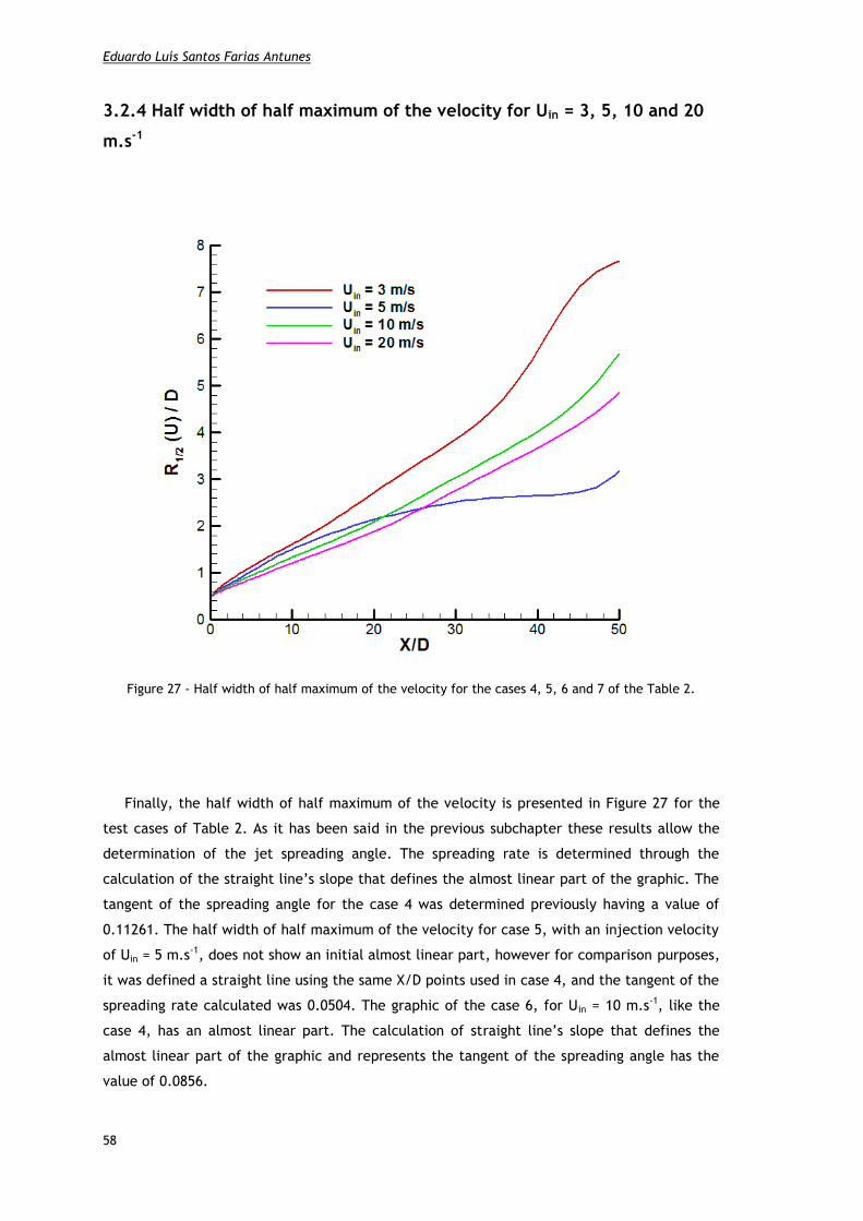
Eduardo Luís Santos Farias Antunes
58
3.2.4 Half width of half maximum of the velocity for Uin = 3, 5, 10 and 20
m.s-1
Figure 27 - Half width of half maximum of the velocity for the cases 4, 5, 6 and 7 of the Table 2.
Finally, the half width of half maximum of the velocity is presented in Figure 27 for the
test cases of Table 2. As it has been said in the previous subchapter these results allow the
determination of the jet spreading angle. The spreading rate is determined through the
calculation of the straight line’s slope that defines the almost linear part of the graphic. The
tangent of the spreading angle for the case 4 was determined previously having a value of
0.11261. The half width of half maximum of the velocity for case 5, with an injection velocity
of Uin = 5 m.s-1, does not show an initial almost linear part, however for comparison purposes,
it was defined a straight line using the same X/D points used in case 4, and the tangent of the
spreading rate calculated was 0.0504. The graphic of the case 6, for Uin = 10 m.s-1, like the
case 4, has an almost linear part. The calculation of straight line’s slope that defines the
almost linear part of the graphic and represents the tangent of the spreading angle has the
value of 0.0856.

Evaluation of Numerical Variable Density Approach to Cryogenic Jets
59
The case 7 with an injection velocity of Uin = 20 m.s-1, follows the same trend observed for
case 6, and the graphic has the same evolution however with a lower value of the jet
spreading rate. The tangent of the spreading angle calculated for this case was 0.0790.
As for the results presented above, the injection velocity is one variable that shows to
have a strong influence in the half width of half maximum of the velocity. Analyzing the
Figure 27, manly cases 4, 6 and 7, we can conclude that this influence is made in the way of
reducing the jet spreading angle as the injection velocity increases. Like in the previous two
graphics the case 5 with an injection velocity of Uin = 5 m.s-1 shows not follow the same trend
observed in the other cases.
The analysis of the results obtained in the injection velocity study allows the conclusion
that in fact injection velocity influences the behavior of the jet. In general the increase of
the injection velocity causes a slower change of the jet properties across the axial direction.
Both dense and potential core of the jet growth and the rates of density and velocity decay as
well as the jet spreading rate decrease. One possible explication for this behavior can be the
fact that despite the increase of the injection velocity, the rate of change of the jet
properties does not increase in the temporal reference in the same way that the velocity, and
so, the same values of the jet properties are obtained further downstream as the jet fluid
travels a greater distance in the same length of time.
The case 5 of Table 2 with an injection velocity of Uin = 5 m.s-1 appears in this study as an
exception or an anomaly.

Eduardo Luís Santos Farias Antunes
60

Evaluation of Numerical Variable Density Approach to Cryogenic Jets
61
Chapter 4
Conclusion
The present chapter exhibits the main conclusions achieved in this thesis.
Barata et al. [18] had concluded that the variable density mathematical model could be
successfully used in the study of cryogenic jets injected initially at subcritical temperatures
into an environment at a supercritical temperature over a range of subcritical and
supercritical pressures [18]. The objective of the present work was to extend the study
performed by Barata et al. [18] to lower chamber-to-injection fluid density ratios. Like in
Barata et al. [18], for this investigation an injection of cryogenic liquid nitrogen into a
gaseous nitrogen environment was simulated.
The major parameter of comparison between the results obtained in this work and others
experimental and numerical works was the jet growth rate. It is important to refer that the
computation model was not written for the study of liquid injections into gaseous ambient,
but instead to study incompressible variable density gaseous jets. The test conditions imposed
in the present work are completely outside of the range of application for which the
computational model was though. However, it was conclude that for the three test cases the
jet spreading angle obtained by the variable density approach are in general agreement with
the experimental and modeling result of Chehroudi et al.[23]. These results show the
capability of the incompressible variable density computational model to study cryogenic
jets, injected initially at subcritical temperatures into an environment at a supercritical
temperature over a range of subcritical pressures.
The study of conditions with lower density ratios allowed finding the limit of applicability
of the incompressible variable density approach. It was verified that for density ratios bellow
ω = 0.025 the computational model shows a dramatic change in the jet behavior and the
results obtained for these conditions not fit with any experimental or numerical results
obtained by other authors. This was the major conclusion achieved in the present thesis.
The study of the injection velocity in the jet behavior, despite being an investigation with
less relevance in the present thesis, also allowed some interesting conclusions. It was found
that for this computational model, a change in the injection velocity produces some
differences in jet behavior. Moreover, it was verified a general trend that an increase in the
injection velocity is responsible slower variation of the jet properties across the domain of
study, however this conclusion is not observable in all the studied injection velocities. A
further more complete analysis of the jet injection velocity influence in the jet behavior
could be an interesting subject for a future investigation.

Eduardo Luís Santos Farias Antunes
62
Evaluation of Numerical Variable Density Approach to Cryogenic Jets
63
References
[1] - Chehroudi, B., Cohn, R., and Talley, D., “Visual Characteristics and Initial Growth Rates
of Round Cryogenic Jets at Subcritical and Supercritical Pressures,” Physics of Fluids, Vol. 14,
No. 2, 2002, pp. 850-861.
[2] - Bellan, J., “Supercritical (and Subcritical) Fluid Behavior and Modeling: Drops, Streams,
Shear and Mixing Layers, Jets and Sprays,” Progress in Energy and Combustion Science, Vol.
26, Issues 4-6, 2000, pp. 329-366.
[3] - Yang, V., “Modeling of Supercritical Vaporization, Mixing, and Combustion Processes in
Liquid-Fueled Propulsion Systems,” Proceedings Of the Combustion Institute, Vol. 28, 2000,
pp. 925-942.
[4] – Segal, C., and Polikhov, S.A., “Subcritical to Supercritical Mixing,” Physics of Fluids, Vol.
20, Issue 5, 2008, pp. 052101-1-052101-7.
[5] – Oschwald, M., Smith, J. J., Branam, R., Hussong, J., Schik, A., Chehroudi, B. and Talley,
D. (2006) “Injection of Fluids into Supercritcal Environments,” Combustion Science and
Technology, Vol. 178, No. 1-3, 2006, pp. 49-100.
[6] - Mayer, W.O.H., Schick, A. H. A., Vielle, B., Chauveau, C., Gökalp, I., Talley, D.G., and
Woodward, R.D., “Atomization and Breakup of Cryogenic Propellants under High-Pressure
Subcritical and Supercritical Conditions,” Journal of Propulsion and Power, Vol.14, No.5,
1998, pp.835-842.
[7] - Chehroudi, B., Cohn, R., and Talley, D., “Cryogenic Shear Layers: Experiments and
Phenomenological Modeling of the Initial Growth Rate under Subcritical and Supercritical
Conditions,” International Journal of Heat and Fluid Flow, Vol. 23, Issue 5, 2002, pp. 554-
563.
[8] – Givler, S.D., John Abraham, J., “Supercritical Droplet Vaporization and Combustion
Studies,” Progress in Energy and Combustion Science, Vol. 22, Issue 1, 1996, pp. 1-28.
[9] – Zhang, H., Raghavan, V., Gogos, G., “Subcritical and Supercritical Droplet Evaporation
within a Zero-Gravity Environment: Low Weber Number Relative Motion,” International
Communications in Heat and Mass Transfer, Vol. 35, Issue 4, 2008, pp. 385–394.

Eduardo Luís Santos Farias Antunes
64
[10] – Nomura, H., Ujiie, Y., Rath, H.J., Sato, J., Kono, M., “Experimental Study of High-
Pressure Droplet Evaporation using Microgravity Conditions,” Twenty-Sixth Symposium
(International) on Combustion/The Combustion Institute, 1996, pp. 1267–1273.
[11] – Tsue, M., Nomur, H., Niwa, M., Miyano, H., Sato, J., Kono, M., “Evaporation of a Fuel
Droplet in a High Pressure High Temperature Atmosphere,” Japan Society for Aeronautical
and Space Sciences, Journal (ISSN 0021-4663), Vol. 37, No. 420, 1989, pp. 21-28.
[12] – Fieberg, C., Reichelt, L., Martin, D., Renz, U., and Kneer, R., “Experimental and
Numerical Investigation of Droplet Evaporation under Diesel Engines Conditions,”
International Journal of Heat and Mass Transfer, Vol. 52, Issues 15-16, 2009, pp. 3738-3746.
[13] - Zhu, G.S., and Aggarwal, S.K., “Transient Supercritical Droplet Evaporation with
emphasis on the Effects of Equation of State”, International Journal of Heat and Mass
Transfer, Vol. 43, Issue 7, 2000, pp. 1157-1171.
[14] – Emekwuru, N.G., Watkins, P., “Analysis of a Two-Fluid Sprayer and its Use to Develop
the Number Size Distribution Moments Spray Model Part II: Computational Analysis,”
Atomization and Sprays, Vol. 20, Issue 8, 2010, pp. 653-672.
[15] - Oschwald, M., and Schik, A., “Supercritical Nitrogen Free Jet Investigated by
Spontaneous Raman Scattering,” Experiments in Fluids, Vol. 27, No. 6, 1999, pp. 497-506.
[16] – Mayer, W., and Telaar, J., “Investigation of Breakup of Turbulent Cryogenic Variable-
Density Jets,” Atomization and Sprays, Vol. 12, Issue 5-6, 2002, pp. 651-666.
[17] - Sanders, J. P. H., B. Sarh, B., Gokalp, I., “Variable Density Effects in Axisymmetric
Isothermal Turbulent jets: a Comparison Between a First- and a Second-order Turbulence
Model,” Int. J. Heat Mass Transfer. Vol. 40, No. 4, 1997, pp. 823-842.
[18] – Barata, J.M.M., Gokalp, I., Silva, A.R.R., “Numerical Study of Cryogenic Jets under
Supercritical Conditions,” Journal of Propulsion and Power, Vol. 19, No.1, 2003, pp. 142-147.
[19] - Zong, N., Meng, H., Hsieh, S., and Yang, V., “A Numerical Study of Cryogenic Fluid
Injection and Mixing under Supercritical Conditions,” Physics of Fluids, Vol. 16, No. 12, 2004,
pp. 4248-4261.
[20] - Sierra-Pallares, J., Parra-Santos, M.T., García-Serna, J., Castro, F., Cocero, M.J.,
“Numerical Analysis of High-pressure Fluid Jets: Application to RTD Prediction in Supercritical
Reactors,” Journal of Supercritical Fluids, Vol. 49, Issue 2, 2009, pp. 249-255.

Evaluation of Numerical Variable Density Approach to Cryogenic Jets
65
[21] - Schmitt, T., Selle, L., Cuenot, B., and Poinsot, T., “Large-Eddy Simulation of
Transcritical Flows,” Comptes Rendus Mécanique, Vol. 337, Issues 6-7, June-July 2009, pp.
528-538.
[22] – Kim, T., Kim, Y., Kim, S., “Numerical study of cryogenic liquid nitrogen jets at
supercritical pressures,” The Journal of Supercritical Fluids, Vol. 56, Issue 2, 2011, pp. 152-
163.
[23] – Chehroudi, B., Cohn, R., and Talley, D., “Spray/Gas Behaviour of Cryogenic Fluids
under Sub- and Supercritical Conditions,” Eighth International Conference on Liquid
Atomization & Sprays Systems, ICLASS-2000, Pasadena, California, USA, July 16-20, 2000.

Eduardo Luís Santos Farias Antunes
66

Attachment 1
Extended Abstract send to AIAA

American Institute of Aeronautics and Astronautics
1
Evaluation of Numerical Variable Density Approach to
Cryogenic Jets
Eduardo L.S.F. Antunes1, André R. R. Silva
2, Jorge M. M. Barata
3
Universidade da Beira Interior, Covilhã, 6201-1, Portugal
Abstract Fuel injection presents itself as one of the great challenges in engineering of diesel engines, gas
turbines and rocket engines, combining in the last one also the injection of oxidizer. It is widely known
that the increase of operating pressure and temperatures in combustion chamber, or thrust chamber in
rocket engines, leads to an increase of engine efficiency, reducing this way the fuel consumption. Thereby
is a general trend in new engine designs to operate with higher chamber pressures and temperatures. Also
the appearance of new and more resistant materials is other reason that could make grow this tendency.
As a result of these increasingly higher pressures, the injected fluids may experience ambient conditions
exceeding the critical values. The Space Shuttle Main Engine and the Vulcain with thrust chamber
pressures of respectively 22.3 MPa and 28.2 MPa are both examples of engines in which the chamber
pressure exceeds the critical pressure of Pcr = 5.043 MPa for liquid oxygen and Pcr = 1.28 MPa for liquid
hydrogen1. In these application, the initial temperature of the oxygen can initially be below the critical
temperature of the oxygen (Tcr = 154.58 K) but it then undergoes to a transition, when in the combustion
chamber, reaching supercritical temperatures. At these conditions the liquid fuel is on supercritical
conditions and its physical state is named as fluid. As the fluid reach pressure and temperature values
exceeding the critical ones it suffers significantly changes in its properties. The effective mass diffusivity,
the surface tension and the latent heat of the liquid all vanish in critical conditions. On the other hand, the
heat capacity at constant pressure, Cp, the isentropic compressibility, κs, and the thermal conductivity, λ ,
all become infinite [2]. These changes in the fluid behaviour cause the inapplicability of the traditional
two-phase flow models used in fuel injection under subcritical conditions, thus there is a need to develop
new models with can correctly be applied to supercritical fuel injection.
Several authors investigated the fuel injection in supercritical condition both in experimentally and
numerically3-22
. The first experimental investigations performed had as principal objective the study of the
visual structure of the jet without obtaining any quantitative result1, 6
, these investigations observed that
the jet structure suffers significantly changes as the pressure increases, firstly the surface tension
reduction leads to the formations of jet ligaments and droplets that detach from the main jet structure and
a further increase of the chamber pressure into supercritical conditions leads to gas-gas like structure of
the jet. More recent experimental work made quantitative studies in which results like the jet spreading
angle, density and temperature were obtained4,7,15,16
. These quantitative experimental results allowed the
comparison with the results obtained in numerical studies and this way validate the numerical models17-22
.
Barata et al.18
performed an initial investigation aimed to evaluate the capabilities of a computational
method developed for incompressible but variable density flows when applied to supercritical conditions.
Their results have show a good agreement with the experimental data, but they only considered
intermediate density ratios from 0.05 to 0.14. The present work extend the investigation of Ref. 18 to
much lower density ratios and investigates the limits of application of the variable density approach to
supercritical jets.
The flow configuration is the same used before experimentally1,7
and numerically18
and is shown in
Figure 1. A cryogenic nitrogen jet (LN2) is injected initially at subcritical temperature of 100-110 K into
an environment at an ambient temperature (300 K) gaseous nitrogen (GN2) but in this work is only over a
range of subcritical pressures close to the critical value.
The reduced pressure Pr which is defined as the ratio of the chamber pressure to the critical pressure
(Pcritical = 3.39 Mpa; Tcritical = 126.2 K) in this work is change between Pr = 0.583 and Pr = 0.825.
The computational method was developed to solve variable density jet flows, and is based on the
solution of the conservation equations for momentum and mass. Turbulence is modelled with the “k~”
turbulence model. In the conservation equations, mass weighted averaging is applied to avoid the
appearance of many terms involving density fluctuations for which additional models are needed. To
describe mixing of gases, the mixture fraction F, which represents the mass fraction of the nozzle fluid, is
1 MEng Student, Aerospace Sciences Department, Rua Marques Avila e Bolama.
2 Assistant Professor, Aerospace Sciences Department, AIAA Member.
3 Full Professor, Aerospace Sciences Department, Associate Fellow of AIAA.

American Institute of Aeronautics and Astroneutics
2
introduced. The approach adopted here has been applied to variable density jets and its performance and
limits of applicability are evaluated for lower density ratios.
The typical velocity and scalar field of the jet for lower density ratios are shows in Figure 2. For this
figure was chosen the case with a density ratio of ω = 0.025 which is the studied case with the lower
density ratio. This case corresponds to a liquid nitrogen injection at a temperature of 100K into an
environment at a pressure of 0.583Pcr and a temperature of 300K. The velocity field shows the formation
of a vortex above the jet and some divergence of the jet is visible after a length of approximately 0.004 m
due to the vortex. The density suffers a rapid decrease near the injector with the jet reaching the ambience
density in a very small length, the mixture fraction also shows a rapid decrease, although slower than the
density decrease.
The Figure 3 shows the axial velocity for the tree different chamber pressures, it is observed bigger
velocity decay for de case with higher chamber pressure, this can indicate a smaller jet penetration in the
case with higher pressure.
The jet spreading is determined by the full width at half maximum of velocity profile and it is showed
in Figure 4. Numerical results show a slightly decrease of the jet spreading angle as the pressure increases
in the subcritical pressure ranges.
Figure 5 shows the influence of the chamber-to-injectant density ratio into jet spray or mixing layer
divergence angle. The results obtained agree relatively well with both the experimental measurements for
the LN2 injection into GN2 environment. The present results are also shown in Figure 5, and revel that the
variable density approach does not offers valid data for density ratios below ω = 0.025.
References 1Chehroudi, B., Cohn, R., and Talley, D., “Visual Characteristics and Initial Growth Rates of Round Cryogenic
Jets at Subcritical and Supercritical Pressures,” Physics of Fluids, Vol. 14, No. 2, 2002, pp. 850-861. 2Bellan, J., “Supercritical (and Subcritical) Fluid Behavior and Modeling: Drops, Streams, Shear and Mixing
Layers, Jets and Sprays,” Progress in Energy and Combustion Science, Vol. 26, Issues 4-6, 2000, pp. 329-366. 3Yang, V., “Modeling of Supercritical Vaporization, Mixing, and Combustion Processes in Liquid-Fueled
Propulsion Systems,” Proceedings Of the Combustion Institute, Vol. 28, 2000, pp. 925-942. 4Segal, C., and Polikhov, S.A., “Subcritical to Supercritical Mixing,” Physics of Fluids, Vol. 20, Issue 5, 2008,
pp. 052101-1-052101-7. 5Oschwald, M., Smith, J. J., Branam, R., Hussong, J., Schik, A., Chehroudi, B. and Talley, D. (2006)
“INJECTION OF FLUIDS INTO SUPERCRITICAL ENVIRONMENTS”, Combustion Science and Technology,
178: 1, 49-100. 6Mayer, W.O.H., Schick, A. H. A., Vielle, B., Chauveau, C., Gökalp, I., Talley, D.G., and Woodward, R.D.,
“Atomization and Breakup of Cryogenic Propellants under High-Pressure Subcritical and Supercritical Conditions,”
Journal of Propulsion and Power, Vol.14, No.5, 1998, pp.835-842. 7Chehroudi, B., Cohn, R., and Talley, D., “Cryogenic Shear Layers: Experiments and Phenomenological
Modeling of the Initial Growth Rate under Subcritical and Supercritical Conditions,” International Journal of Heat
and Fluid Flow, Vol. 23, Issue 5, 2002, pp. 554-563. 8Givler, S.D., John Abraham, J., “Supercritical Droplet Vaporization and Combustion Studies,” Progress in
Energy and Combustion Science, Vol. 22, Issue 1, 1996, pp. l-28. 9Zhang, H., Raghavan, V., Gogos, G., “Subcritical and Supercritical Droplet Evaporation within a Zero-Gravity
Environment: Low Weber Number Relative Motion,” International Communications in Heat and Mass Transfer,
Vol. 35, Issue 4, 2008, pp. 385–394. 10Nomura, H., Ujiie, Y., Rath, H.J., Sato, J., Kono, M., “Experimental Study of High-Pressure Droplet
Evaporation using Microgravity Conditions,” Twenty-Sixth Symposium (International) on Combustion/The
Combustion Institute, 1996, pp. 1267–1273. 11Tsue, M., Nomur, H., Niwa, M., Miyano, H., Sato, J., Kono, M., “Evaporation of a Fuel Droplet in a High
Pressure High Temperature Atmosphere,” Japan Society for Aeronautical and Space Sciences, Journal (ISSN 0021-
4663), Vol. 37, No. 420, 1989, pp. 21-28. 12Fieberg, C., Reichelt, L., Martin, D., Renz, U., and Kneer, R., “Experimental and Numerical Investigation of
Droplet Evaporation under Diesel Engines Conditions,” International Journal of Heat and Mass Transfer, Vol. 52,
Issues 15-16, 2009, pp. 3738-3746.
13Zhu, G.S., and Aggarwal, S.K., “Transient Supercritical Droplet Evaporation with emphasis on the Effects of
Equation of State”, International Journal of Heat and Mass Transfer, Vol. 43, Issue 7, 2000, pp. 1157-1171.
14Emekwuru, N.G., Watkins, P., "Analysis of a Two-Fluid Sprayer and its Use to Develop the Number Size
Distribution Moments Spray Model Part II: Computational Analysis," Atomization and Sprays, Vol. 20, Issue 8,
2010, pp. 653-672.
15Oschwald, M., and Schik, A., “Supercritical Nitrogen Free Jet Investigated by Spontaneous Raman Scattering,”
Experiments in Fluids, Vol. 27, No. 6, 1999, pp. 497-506.
16Mayer, W., and Telaar, J., “Investigation of Breakup of Turbulent Cryogenic Variable-Density Jets,”
Atomization and Sprays, Vol. 12, Issue 5-6, 2002, pp. 651-666.
17Sanders, J. P. H., B. Sarh, B., Gokalp, I., “Variable Density Effects in Axisymmetric Isothermal Turbulent jets:
a Comparison Between a First- and a Second-order Turbulence Model,” Int. J. Heat Mass Transfer. Vol. 40, No. 4,
1997, pp. 823-842.

American Institute of Aeronautics and Astronautics
3
18Barata, J.M.M., Gokalp, I., Silva, A.R.R., “Numerical Study of Cryogenic Jets under Supercritical Conditions,”
Journal of Propulsion and Power, Vol. 19, No.1, 2003, pp. 142-147. 19Zong, N., Meng, H., Hsieh, S., and Yang, V., “A Numerical Study of Cryogenic Fluid Injection and Mixing
under Supercritical Conditions,” Physics of Fluids, Vol. 16, No. 12, 2004, pp. 4248-4261. 20Sierra-Pallares, J., Parra-Santos, M.T., García-Serna, J., Castro, F., Cocero, M.J., “Numerical Analysis of High-
pressure Fluid Jets: Application to RTD Prediction in Supercritical Reactors”, Journal of Supercritical Fluids, Vol.
49, 2009, pp. 249-255. 21Schmitt, T., Selle, L., Cuenot, B., and Poinsot, T., “Large-Eddy Simulation of Transcritical Flows”, Comptes
Rendus Mécanique, Vol. 337, Issues 6-7, June-July 2009, pp. 528-538. 22Kim, T., Kim, Y., Kim, S., “Numerical study of cryogenic liquid nitrogen jets at supercritical pressures,” The
Journal of Supercritical Fluids, Vol. 56, Issue 2, 2011, pp. 152-163.
Figure 1. Flow configuration

American Institute of Aeronautics and Astroneutics
4
a)
b)
c)
Figure 2. Velocity and scalar fields of the jet with a density ratio of ω = 0.025 and a chamber
pressure of Pr = 0.583, (a) Velocity vectors, (b) Mixture fraction contours, (c) Density contours.

American Institute of Aeronautics and Astronautics
5
Figure 3. Non-dimensional profile of the mean axial velocity, U.
Figure 4. Full width at half maximum of velocity profile.
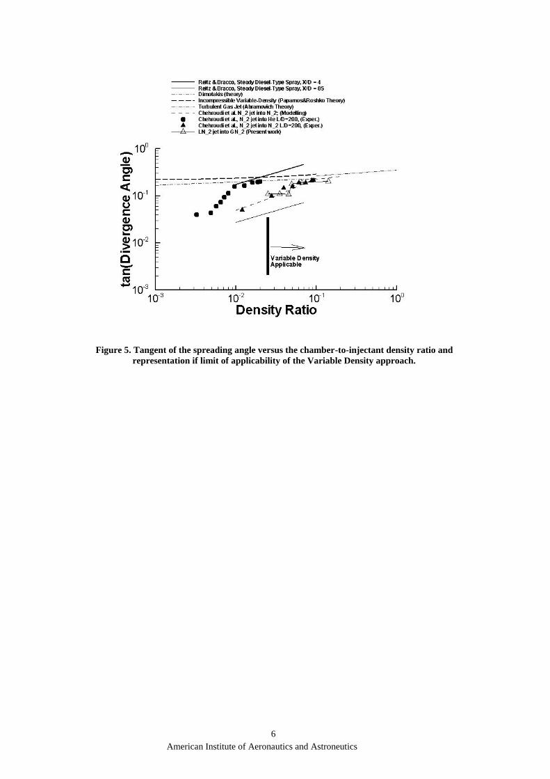
American Institute of Aeronautics and Astroneutics
6
Figure 5. Tangent of the spreading angle versus the chamber-to-injectant density ratio and
representation if limit of applicability of the Variable Density approach.

Attachment 2
Paper send to the International Conference on Engineering UBI2011


1
Application of a Numerical Variable Density Method to cryogenic jets
E.L.S.F. Antunes1, A. R. R. Silva2, J. M. M. Barata3
Universidade da Beira Interior, 6200-001 Covilhã, Portugal
Conference Topic – CT 1
Abstract
The present work is devoted to study cryogenic nitrogen jets in high subcritical conditions. It is a general trend in modern engines the operation in increasingly higher pressures which enhance efficiency. However at higher chamber pressures the injected fluids may experience ambient conditions exceeding the critical values and changing their properties, thus requiring new computational models. Barata et al. [18] performed a numerical investigation evaluating the applicability of an incompressible but variable density model in liquid jets under sub-to-supercritical conditions. The results achieved agree well with the experimental data but they only considered intermediate density ratios. This work extends the investigation of Ref. 18 to lower density ratios. The obtained results agree well with the experimental and numerical data of Chehroudi et al. presented in Ref. 18. It was also found in this work that the computational model does not offers valid results for density ratios below ω = 0.025.
Keywords: Fuel injection; critical point; supercritical conditions; rocket engines; diesel engines; density ratio; jets; variable density.
Nomenclature
B = transfer number βv = evaporation rate Cμ = coefficient in turbulence model d0 = initial droplet diameter d = droplet diameter D = injector diameter [m], normalized
droplet diameter (d(t) / d0) ε = dissipation rate of turbulent energy f = mixture fraction F = mean mixture fraction i = axial direction index j = radial direction index k = turbulent kinetic energy ϕ = generalized variable ω = chamber-to-injection fluid density
ratio (ρ∞/ρ0) Pcr = critical pressure [MPa] P∞ = chamber ambient pressure [MPa] Pr = reduced pressure (P∞/Pcr) ρ = density [kg.m-3] ρ0 = injected fluid density [kg.m-3] ρ∞ = injection chamber’s fluid density
[kg.m−3] r = radial coordinate [m] _____________________________ 1 MEng Student, Aerospace Sciences Department, Rua Marques Avila e Bolama. 2 Assistant Professor, Aerospace Sciences Department, AIAA Member.
3 Full Professor, Aerospace Sciences Department, AIAA Associate Fellow.
Rdiam = injector radius [m] R/D = radial distance normalized by injector diameter Re = Reynolds Number Sϕ = source term t = time [s] T = temperature [K] u = axial velocity [m.s-1] U = mean axial velocity [m.s-1] Uin = injection axial velocity [m.s-1] v = radial velocity [m.s-1] vt = turbulent kinematic viscosity V = mean radial velocity [m.s-1] X = axial coordinate [m] X/D = axial distance normalized by injector diameter
Introduction
Fuel injection presents itself as one of the great challenges in engineering of diesel engines, gas turbines and rocket engines, combining in the last one also the injection of oxidizer. It is widely known that the increase of operating pressure and temperatures in combustion chamber, or thrust chamber in rocket engines, leads to an increase of engine efficiency, reducing this way the fuel consumption. Thereby is a general trend in new engine designs to operate with higher chamber pressures and temperatures. Also the appearance of new and more resistant materials is other reason that could make grow this tendency. As a

result of these increasingly higher pressures, the injected fluids may experience ambient conditions exceeding the critical values. The Space Shuttle Main Engine and the Vulcain with thrust chamber pressures of respectively 22.3 MPa and 28.2 MPa are both examples of engines in which the chamber pressure exceeds the critical pressure of Pcr = 5.043 MPa for liquid oxygen and Pcr = 1.28 MPa for liquid hydrogen1. In these application, the initial temperature of the oxygen can initially be below the critical temperature of the oxygen (Tcr = 154.58 K) but it then undergoes to a transition, when in the combustion chamber, reaching supercritical temperatures. At these conditions the liquid fuel is on supercritical conditions and its physical state is named as fluid. As the fluid reach pressure and temperature values exceeding the critical ones, it suffers significantly changes in its properties. The effective mass diffusivity, the surface tension and the latent heat of the liquid all vanish in critical conditions. On the other hand, the heat capacity at constant pressure, Cp, the isentropic compressibility, κs, and the thermal conductivity, λ, all become infinite [2]. These changes in the fluid behavior cause the inapplicability of the traditional two-phase flow models used in fuel injection under subcritical conditions, thus there is a need to develop new models with can correctly be applied to supercritical fuel injection. Several authors investigated the fuel injection in supercritical condition both in experimentally and numerically3-22. The first experimental investigations performed used techniques like photography and shadowgraphy, and had as principal objective the study of the visual structure of the jet without obtaining any quantitative result1,6, these investigations observed that the jet structure suffers significantly changes as the pressure increases, firstly the surface tension reduction leads to the formations of jet ligaments and droplets that detach from the main jet structure and a further increase of the chamber pressure into supercritical conditions leads to gas-gas like structure of the jet. In more recent experimental works, along with qualitative characterization, were made quantitative studies in which results like the jet spreading angle, density and temperature were obtained4,7,15,16. These quantitative experimental results allowed the comparison with the results obtained in numerical studies and this way validate the numerical models17-22.
Barata et al.18 performed an initial investigation aimed to evaluate the capabilities of a computational method developed for incompressible but variable density flows when applied to supercritical conditions. Their results have show a good agreement with the experimental data, but they only considered intermediate density ratios from 0.05 to 0.14. The present work extends the investigation of Ref. 18 to lower density ratios, corresponding to sub/near-critical conditions, and investigates the limits of application of the variable density approach to supercritical jets. An injection velocity study was also performed in the present work with intend of better characterize the variable density approach.
Mathematical Model
Governing Equations
The method to solve variable density jet
flows is based on the solution of the
conservation equations for momentum and
mass. Turbulence is modeled with the “k~”
turbulence model. A similar method has been
used for three-dimensional or axisymmetric
flows and only the main features are
summarized here.
In the conservation equations, mass
weighted averaging is applied to avoid the
appearance of many terms involving density
fluctuations for which additional models are
needed. A mass averaged quantity is defined
as
~
. (1)
For the governing equations the
standard parabolic truncation is employed.
The mass averaged partial differential
equations governing the steady, variable
density axisymmetric flow may be written in
cylindrical polar coordinates as
r
vur
rx
p
r
UVr
rx
UU
''11~
(2)
r
ww
r
vvr
rx
p
r
VVr
rx
UV ''''11~~
(3)

3
and the continuity equation as
01
r
Vr
rx
U (4)
To describe mixing of gases, the
mixture fraction F, that represents the mass
fraction of the nozzle fluid, is introduced. It
obeys a convection-diffusion equation of the
form
r
fvr
rr
VFr
rx
UF
''11~
(5)
In “k~” turbulence model, the
Reynolds stresses are expressed in terms of
the local strain rate:
j
j
tij
i
j
j
it
x
uk
x
u
x
uj
ui
u~
3
2~~
''~
(6)
with
2kC
t (7)
The scalar flux in equation (5) is
approximated with a gradient transport
assumption
if
t
x
Ff
iu
''
~
(8)
From the foregoing we can deduced
the parabolized set of equations in
cylindrical coordinates where the
generalized equation is
S
dr
~
Drrr
~r
rr
~U
x
11
(9)
where ~
may stand for any of the
velocities, turbulent kinetic energy,
dissipation, or scalar property, and S take
on different values for each particular ~
,
described in detail by Sanders et al17.
The mean density can be obtained from the
mean mixture fraction using the equation
state. With constant pressure this leads to
FF
o
11 (10)
where density fluctuations have been neglected. This is allowed in isothermal jets because the instantaneous density, for which equation (10) is exact, is approximately a linear function of the instantaneous mixture fraction18.
Numerical Method
The governing equations are solved using a parabolized marching algorithm which resembles the (elliptic) TEACH code [17]. The computations are performed by using the continuity equation to obtain the radial velocity (V). Using the radial momentum equation for V and solving a pressure correction equation for V in radial direction did not show any difference with the use of the continuity equation [17]. In this approach the numerical model was applied to variable density jets and for the present case it was used for the study of liquid cryogenic jets under In order to determine the tangent of the jet spreading angle is used the Half Width of Half Maximum of the Velocity (HWHMV), this routine has the function of determine the radial distance from the centerline (r) at which the axial mean velocity (U) is half of the maximum velocity localized in the centerline. This routine analysis all the points in the radial direction comparing them with half of the centerline velocity, when the routine finds a point bellow this value it saves the point before that.
Boundary Conditions There are four boundaries in the computational domain, in these boundaries dependent variables are specified: an inlet and outlet plane, a symmetry axis and a free boundary parallel to the axis. The sensitivity of the solutions to the locations of the boundaries was investigated in previous works, and their final position is sufficiently far away from the jet so that the influence on the computed results is negligible [18]. At the inlet boundary the 1/7th power law turbulent velocity profile was used for the axial velocity at the jet exit.
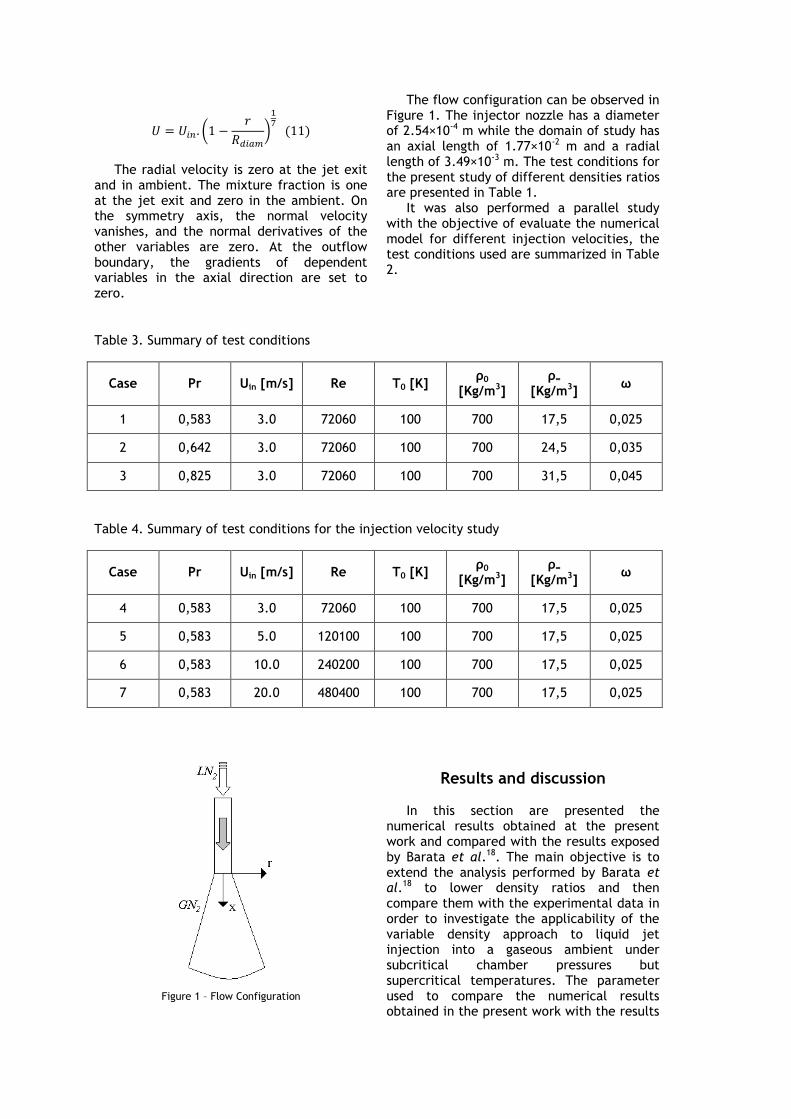
The radial velocity is zero at the jet exit and in ambient. The mixture fraction is one at the jet exit and zero in the ambient. On the symmetry axis, the normal velocity vanishes, and the normal derivatives of the other variables are zero. At the outflow boundary, the gradients of dependent variables in the axial direction are set to zero.
The flow configuration can be observed in Figure 1. The injector nozzle has a diameter of 2.54×10⁻⁴ m while the domain of study has an axial length of 1.77×10⁻² m and a radial length of 3.49×10⁻³ m. The test conditions for the present study of different densities ratios are presented in Table 1. It was also performed a parallel study with the objective of evaluate the numerical model for different injection velocities, the test conditions used are summarized in Table 2.
Table 3. Summary of test conditions
Case Pr Uin [m/s] Re T0 [K] ρ0
[Kg/m3] ρ∞
[Kg/m3] ω
1 0,583 3.0 72060 100 700 17,5 0,025
2 0,642 3.0 72060 100 700 24,5 0,035
3 0,825 3.0 72060 100 700 31,5 0,045
Table 4. Summary of test conditions for the injection velocity study
Case Pr Uin [m/s] Re T0 [K] ρ0
[Kg/m3] ρ∞
[Kg/m3] ω
4 0,583 3.0 72060 100 700 17,5 0,025
5 0,583 5.0 120100 100 700 17,5 0,025
6 0,583 10.0 240200 100 700 17,5 0,025
7 0,583 20.0 480400 100 700 17,5 0,025
Figure 1 – Flow Configuration
Results and discussion In this section are presented the numerical results obtained at the present work and compared with the results exposed by Barata et al.18. The main objective is to extend the analysis performed by Barata et al.18 to lower density ratios and then compare them with the experimental data in order to investigate the applicability of the variable density approach to liquid jet injection into a gaseous ambient under subcritical chamber pressures but supercritical temperatures. The parameter used to compare the numerical results obtained in the present work with the results

5
Figure 2 - Velocity and scalar fields of the jet with a density ratio of ω = 0.025 and a chamber pressure of Pr = 0.583, (a) Velocity vectors, (b) Mixture fraction contours, (c) Density contours.

Figure 3 - Velocity and scalar fields of the jet with a density ratio of ω = 0.035 and a chamber pressure of Pr = 0.642, (a) Velocity vectors, (b) Mixture fraction contours, (c) Density contours.

7
exposed in Ref. 18 is the jet growth rate. The jet growth rate is calculated by the tangent of the half with of half maximum of the velocity (HWHMV), this parameter is given by the calculation at each axial point of the radial distance to the centerline at which the axial velocity (U) is half of the velocity at the centerline. However other parameters were used in the characterization of the jet allowing also some interesting conclusions and are shown in the present paper. Figures 2 and 3 show the typical velocity and scalar fields of the jet for test conditions 1 (Figure 2) and 3 (Figure 3) of Table 1. In both cases the jet structure is very similar, in the velocity field is visible the appearance of the entrainment phenomena close to the injector, with the jet fluid dragging the ambient fluid. This phenomenon causes the appearance of a vortex above the jet. It appears that the position of the center of the vortex is influenced by the density ratio, when the density ratio increases the vortex center moves downstream. The mixture fraction and density scalar field show the rapid change of the jet structure at the injector exit. The density scalar field shows a faster decrease after the injector than the mixture fraction scalar field. This suggests that the density rapid decreased is not caused by the mixture of the injected fluid with the less dense ambient fluid but indeed by a rapid expansion that the injected fluid may experiences as it exits the injector.
Figure 4 – Axial variation of the centerline density.
Figure 4 shows the axial variation of the centerline density in a logarithmic scale for cases 1 to 3 of Table 1. It is visible that the centerline density has a very similar behavior
for the three cases with a first stage of almost constant density followed by a stage with a fast decrease of the centerline density and then stabilization around the ambient density value. A closer look to the graphic allows however to perceive that the case with a higher ambient pressure has a slightly higher decrease rate which is in agreement with the density scalar field observed in Figures 2 and 3. The length of the potential core based on the density is defined by the initial, almost constant, stage of the axial variation of the centerline density which lasts until an approximately length of X/D = 3 diameters for the three studied cases.
Figure 5 – Centerline velocity decay.
The centerline velocity decay is shown in Figure 5 for the cases 1, 2 and 3. The velocity decay has a similar profile for the three cases with a first stage with almost no decay followed by a stage with a higher rate of decay and finally a stabilization like observed in Figure 4 for the variation of density. A higher rate of velocity decay is observed for the cases with higher ambient pressure indicating a greater interaction between the injection and ambient fluids. The length of the potential core based on the velocity decay is defined in the present work by the axial distance to the injector at which the centerline velocity has decayed 10%. The length of the potential core is between X/D = 7.9 and X/D = 7.47 diameters respectively for cases 1 and 3. Thus it is verified that the length of the potential core based on centerline velocity decay has a substantially different value that the approximately X/D = 3 diameters found for the potential core based on the centerline density. This is an

Figure 6 – Half width of half maximum of the velocity.
Figure 7 – Decay rate of the centerline velocity and density.

9
interesting result, as in previous works the length of the potential core based on the density has approximately the same value as the one based on the velocity decay, and hypothesizes that the injected, possibly identify by the observation of the scalar fields, may contribute with kinetic energy to the jet. Figure 6 shows the half width of the half maximum of the velocity (HWHMV) for the cases 1, 2 and 3 of Table 1. The three cases have a similar evolution of the HWHMV across the domain of study with an almost linear first stage and a second non linear stage. The tangent of the slope of the almost linear stage corresponds to the jet growing rate. Observing the graphic it is possible to conclude that the jet growing rate is very similar for the three studied cases with only
a slightly decrease as the chamber pressure increases. This was however not an expected result as in several previous work the increase of the chamber pressure causes an increase in the jet growing rate. In Figure 7 are shown the decay rates of velocity and density after the potential core for the cases of Table 1. For both velocity and density an increase in the injection chamber pressure has as result an increase of the decay rate which is in agreement with previous works from other authors, however this effect is more pronounced in the velocity decay. The velocity also shows for the three cases a higher decay rate then the density although is important to remember that the density decay starts earlier then the velocity decay due to the longer potential core obtained for the velocity.
Figure 8 - Tangent of the spreading angle versus the chamber-to-injectant density ratio and representation if limit of applicability of the Variable Density approach.

Figure 8 is similar to the graphic presented by Barata et al.18 and shows the tangent of the jet spreading angle, calculated by the half width of half maximum of the velocity, in order to the density ratio. In addition to the three cases of Table 1 the graphic contains also results obtained by other authors in previous investigations including the results of Barata et al.18, the investigation which the present work pretends to extend. The results achieved in the present work are represented in red while those achieved by other authors are represented in black. Obversing the graphic it is visible that the result obtained for a density ratio of ω = 0.025 agree very well with the experimental result obtained by Chehroudi et al.23, the result obtained for a density ω = 0.035 is in total agreement with the modeling results of the same author. The ω = 0.045 density ratio case shows a slight divergence from previous result but is still very close to the modeling result of Chehroudi et al.23. The test of the present variable density approach to lower density ratios, which are not presented here, allow the conclusion that the density ratio of ω = 0.025 is the lowest value liable to be modeled by the present mathematical model. This conclusion is represented in Figure 8 by the vertical red line that marks the limit of applicability of the variable density approach. The influence of the injection velocity in jet behavior was also subject of analysis at the present investigation. The objective was to perform a better characterization of the mathematical model. In order to achieve this objective the variable density approach was tested for different injection velocities as presented in Table 2. Figure 9 shows the velocity and scalar fields for the test case 7 of Table 2. It is visible that the jet has the same structure found in Figure 2 corresponding to the case 4 of Table 2. It’s however possible to verify that the vortex center appears in localization further downstream, also the mixture fraction and density show a slower evolution across the centerline when compared with the case with slower injection velocity. The axial variation of the centerline density shown in Figure 10 corroborates the observation stated above. The centerline density shows a slower decrease for higher injection velocities. One interesting observation is the increase of the potential core based on density as the injection velocity increases. Similar observations are made for the centerline velocity decay. As
the injection velocity increases the potential core based on the velocity decay increases and the centerline velocity shows a lower rate of decay, this is somehow contrary to the expected since an increase in the injection velocity should lead to an increase of drag forces between the injected and the ambient fluid and this way increase the velocity decay rate. Like in the axial variation of the centerline also for the centerline velocity decay the case 5 with an injection velocity of Uin = 5 m.s-1 shows a behavior different from the tendency followed by the other three cases. The half width of half maximum of the velocity is shown in Figure 11. Again the case 4 of Table 2 shows a different HWHMV structure then the other three cases not having an almost linear stage. By the observation of the graphic can be concluded that an increase of the injection velocity causes a decrease in the jet spreading angle.
Conclusions Barata et al. [18] had concluded that the variable density mathematical model could be successfully used in the study of cryogenic jets injected initially at subcritical temperatures into an environment at a supercritical temperature over a range of subcritical and supercritical pressures [18]. The objective of the present work was to extend the study performed by Barata et al. [18] to lower chamber-to-injection fluid density ratios. Like in Barata et al. [18], for this investigation an injection of cryogenic liquid nitrogen into a gaseous nitrogen environment was simulated. In the analysis of the obtained result were identified some interesting new results. The fastest mixture fraction scalar field evolution when compared with the density scalar field together with the difference between the potential core based on density and the one based on velocity decay, suggests that a vigorous expansion of the injected fluid happens as it enters the injection chamber. And the longer potential core based on the velocity decay indicated that expansion may somehow contribute with kinetic energy to the jet. The results of the half with of half maximum of the velocity allowed the determination of the jet growth rate with are in general agreement with the results obtained by Chehroudi et al.23 described in Ref. 18. By the analysis of the results of the HWHMV obtained to density ratios lower than

11
ω = 0.025, it was concluded that below this value no more agreement was found with previous experimental and numerical results. This establishes the limit of applicability of the variable density approach to cryogenic liquid jet into a supercritical temperature and subcritical pressure ambient.
References
1Chehroudi, B., Cohn, R., and Talley, D., “Visual
Characteristics and Initial Growth Rates of Round Cryogenic Jets at Subcritical and Supercritical Pressures,” Physics of Fluids, Vol. 14, No. 2, 2002, pp. 850-861.
2Bellan, J., “Supercritical (and Subcritical) Fluid Behavior and Modeling: Drops, Streams, Shear and Mixing Layers, Jets and Sprays,” Progress in Energy and Combustion Science, Vol. 26, Issues 4-6, 2000, pp. 329-366.
3Yang, V., “Modeling of Supercritical Vaporization, Mixing, and Combustion Processes in Liquid-Fueled Propulsion Systems,” Proceedings Of the Combustion Institute, Vol. 28, 2000, pp. 925-942.
4Segal, C., and Polikhov, S.A., “Subcritical to Supercritical Mixing,” Physics of Fluids, Vol. 20, Issue 5, 2008, pp. 052101-1-052101-7.
5Oschwald, M., Smith, J. J., Branam, R., Hussong, J., Schik, A., Chehroudi, B. and Talley, D. (2006) “INJECTION OF FLUIDS INTO SUPERCRITICAL ENVIRONMENTS”, Combustion Science and Technology, 178: 1, 49-100.
6Mayer, W.O.H., Schick, A. H. A., Vielle, B., Chauveau, C., Gökalp, I., Talley, D.G., and Woodward, R.D., “Atomization and Breakup of Cryogenic Propellants under High-Pressure Subcritical and Supercritical Conditions,” Journal of Propulsion and Power, Vol.14, No.5, 1998, pp.835-842.
7Chehroudi, B., Cohn, R., and Talley, D., “Cryogenic Shear Layers: Experiments and Phenomenological Modeling of the Initial Growth Rate under Subcritical and Supercritical Conditions,” International Journal of Heat and Fluid Flow, Vol. 23, Issue 5, 2002, pp. 554-563.
8Givler, S.D., John Abraham, J., “Supercritical Droplet Vaporization and Combustion Studies,” Progress in Energy and Combustion Science, Vol. 22, Issue 1, 1996, pp. l-28.
9Zhang, H., Raghavan, V., Gogos, G., “Subcritical and Supercritical Droplet Evaporation within a Zero-Gravity Environment: Low Weber Number Relative Motion,” International Communications in Heat and Mass Transfer, Vol. 35, Issue 4, 2008, pp. 385–394.
10Nomura, H., Ujiie, Y., Rath, H.J., Sato, J., Kono, M., “Experimental Study of High-Pressure Droplet Evaporation using Microgravity Conditions,” Twenty-Sixth Symposium (International) on Combustion/The Combustion Institute, 1996, pp. 1267–1273.
11Tsue, M., Nomur, H., Niwa, M., Miyano, H., Sato, J., Kono, M., “Evaporation of a Fuel Droplet in a High Pressure High Temperature Atmosphere,” Japan Society for Aeronautical and Space Sciences, Journal (ISSN 0021-4663), Vol. 37, No. 420, 1989, pp. 21-28.
12Fieberg, C., Reichelt, L., Martin, D., Renz, U., and Kneer, R., “Experimental and Numerical Investigation of Droplet Evaporation under Diesel Engines Conditions,” International Journal of Heat and Mass Transfer, Vol. 52, Issues 15-16, 2009, pp. 3738-3746.
13Zhu, G.S., and Aggarwal, S.K., “Transient Supercritical Droplet Evaporation with emphasis on the Effects of Equation of State”, International Journal of Heat and Mass Transfer, Vol. 43, Issue 7, 2000, pp. 1157-1171.
14Emekwuru, N.G., Watkins, P., "Analysis of a Two-Fluid Sprayer and its Use to Develop the Number Size Distribution Moments Spray Model Part II: Computational Analysis," Atomization and Sprays, Vol. 20, Issue 8, 2010, pp. 653-672.
15Oschwald, M., and Schik, A., “Supercritical Nitrogen Free Jet Investigated by Spontaneous Raman Scattering,” Experiments in Fluids, Vol. 27, No. 6, 1999, pp. 497-506.
16Mayer, W., and Telaar, J., “Investigation of Breakup of Turbulent Cryogenic Variable-Density Jets,” Atomization and Sprays, Vol. 12, Issue 5-6, 2002, pp. 651-666.
17Sanders, J. P. H., B. Sarh, B., Gokalp, I., “Variable Density Effects in Axisymmetric Isothermal Turbulent jets: a Comparison Between a First- and a Second-order Turbulence Model,” Int. J. Heat Mass Transfer. Vol. 40, No. 4, 1997, pp. 823-842.
18Barata, J.M.M., Gokalp, I., Silva, A.R.R., “Numerical Study of Cryogenic Jets under Supercritical Conditions,” Journal of Propulsion and Power, Vol. 19, No.1, 2003, pp. 142-147.
19Zong, N., Meng, H., Hsieh, S., and Yang, V., “A Numerical Study of Cryogenic Fluid Injection and Mixing under Supercritical Conditions,” Physics of Fluids, Vol. 16, No. 12, 2004, pp. 4248-4261.
20Sierra-Pallares, J., Parra-Santos, M.T., García-Serna, J., Castro, F., Cocero, M.J., “Numerical Analysis of High-pressure Fluid Jets: Application to RTD Prediction in Supercritical Reactors”, Journal of Supercritical Fluids, Vol. 49, 2009, pp. 249-255.
21Schmitt, T., Selle, L., Cuenot, B., and Poinsot, T., “Large-Eddy Simulation of Transcritical Flows”, Comptes Rendus Mécanique, Vol. 337, Issues 6-7, June-July 2009, pp. 528-538.
22Kim, T., Kim, Y., Kim, S., “Numerical study of cryogenic liquid nitrogen jets at supercritical pressures,” The Journal of Supercritical Fluids, Vol. 56, Issue 2, 2011, pp. 152-163.
23Chehroudi, B., Cohn, R., and Talley, D., “Spray/Gas Behaviour of Cryogenic Fluids under Sub- and Supercritical Conditions”, Eighth International Conference on Liquid Atomization & Sprays Systems, ICLASS-2000, Pasadena, California, USA, July 16-20, 2000.


Attachment 3
Paper send to AIAA


1
American Institute of Aeronautics and Astronautics
EVALUATION OF NUMERICAL VARIABLE DENSITY APPROACH TO CRYOGENIC JETS
E.L.S.F. Antunes1, A. R. R. Silva
2, J. M. M. Barata
3
Universidade da Beira Interior, 6200-001 Covilhã, Portugal
The present work is devoted to study cryogenic nitrogen jets in high subcritical conditions. Fuel injection is
one of the great challenges in engineering of diesel engines, gas turbines and rocket engines, combining in the
last one also the injection of oxidizer. It is widely known that the increase of operation pressures and
temperatures increases engine efficiency and reduces fuel specific consumption. Thus, it is a general trend in
modern engines the operation in increasingly higher pressures. However at higher chamber pressures the
injected fluids may experience ambient conditions exceeding the critical values. Several authors stated that at
these conditions the injected fluids suffers a change of its properties, and the traditional two-phase flow models
cannot correctly predict the jet behavior at these conditions, thus new computational models are needed for
these specific conditions. Barata et al. [18] performed a numerical investigation aimed to evaluate the
applicability of an incompressible but variable density model in liquid jets under sub-to-supercritical
conditions. The results achieved agree well with the experimental data but they only considered intermediate
density ratios from 0.05 to 0.14. The objective of the present work was to extend the investigation of Ref. 18 to
lower density ratios from 0.025 to 0.045 which correspond to cases with subcritical chamber pressures. The
obtained results agree well with the experimental and numerical data of Chehroudi et al. presented in Ref. 18.
It was also found in this work that the computational model does not offers valid results for density ratios.
Nomenclature
B = transfer number
βv = evaporation rate
Cμ = coefficient in turbulence model
d0 = initial droplet diameter
d = droplet diameter
D = injector diameter [m], normalized
droplet diameter (d(t) / d0)
ε = dissipation rate of turbulent energy
f = mixture fraction
F = mean mixture fraction
i = axial direction index
j = radial direction index
k = turbulent kinetic energy
ϕ = generalized variable
ω = chamber-to-injection fluid density ratio
(ρ∞/ρ0)
Pcr = critical pressure [MPa]
P∞ = chamber ambient pressure [MPa]
Pr = reduced pressure (P∞/Pcr)
ρ = density [kg.m-3
]
ρ0 = injected fluid density [kg.m-3
]
ρ∞ = injection chamber’s fluid density
[kg.m−3
]
r = radial coordinate [m]
_____________________________ 1 MEng Student, Aerospace Sciences Department,
Rua Marques Avila e Bolama. 2 Assistant Professor, Aerospace Sciences
Department, AIAA Member. 3 Full Professor, Aerospace Sciences Department, AIAA
Associate Fellow.
R/D = radial distance normalized by injector
diameter
Rdiam = injector radius [m]
Re = Reynolds Number
Sϕ = source term
t = time [s]
T = temperature [K]
u = axial velocity [m.s-1
]
U = mean axial velocity [m.s-1
]
Uin = injection axial velocity [m.s-1
]
v = radial velocity [m.s-1
]
vt = turbulent kinematic viscosity
V = mean radial velocity [m.s-1
]
X = axial coordinate [m]
X/D = axial distance normalized by injector
diameter
Introduction
Fuel injection presents itself as one of the great
challenges in engineering of diesel engines, gas
turbines and rocket engines, combining in the last
one also the injection of oxidizer. It is widely
known that the increase of operating pressure and
temperatures in combustion chamber, or thrust
chamber in rocket engines, leads to an increase of
engine efficiency, reducing this way the fuel
consumption. Thereby is a general trend in new
engine designs to operate with higher chamber
pressures and temperatures. Also the appearance of
new and more resistant materials is other reason
that could make grow this tendency. As a result of
these increasingly higher pressures, the injected
fluids may experience ambient conditions
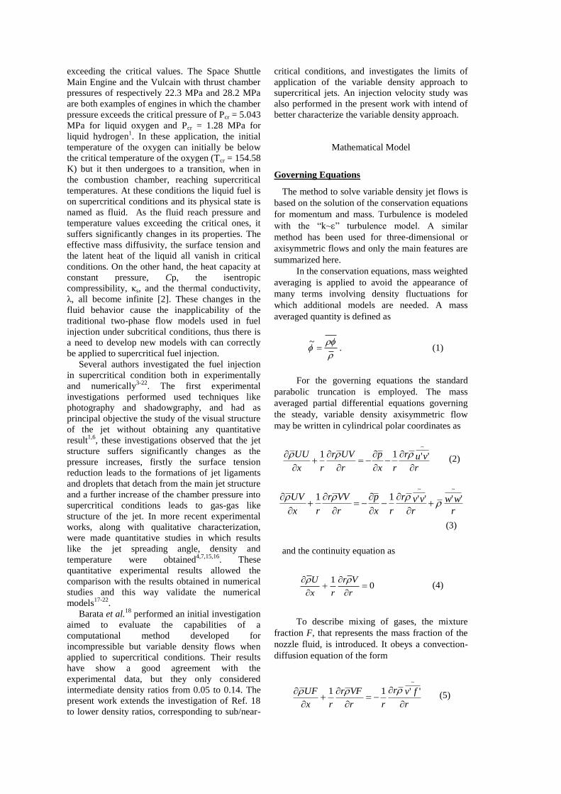
exceeding the critical values. The Space Shuttle
Main Engine and the Vulcain with thrust chamber
pressures of respectively 22.3 MPa and 28.2 MPa
are both examples of engines in which the chamber
pressure exceeds the critical pressure of Pcr = 5.043
MPa for liquid oxygen and Pcr = 1.28 MPa for
liquid hydrogen1. In these application, the initial
temperature of the oxygen can initially be below
the critical temperature of the oxygen (Tcr = 154.58
K) but it then undergoes to a transition, when in
the combustion chamber, reaching supercritical
temperatures. At these conditions the liquid fuel is
on supercritical conditions and its physical state is
named as fluid. As the fluid reach pressure and
temperature values exceeding the critical ones, it
suffers significantly changes in its properties. The
effective mass diffusivity, the surface tension and
the latent heat of the liquid all vanish in critical
conditions. On the other hand, the heat capacity at
constant pressure, Cp, the isentropic
compressibility, κs, and the thermal conductivity,
λ, all become infinite [2]. These changes in the
fluid behavior cause the inapplicability of the
traditional two-phase flow models used in fuel
injection under subcritical conditions, thus there is
a need to develop new models with can correctly
be applied to supercritical fuel injection.
Several authors investigated the fuel injection
in supercritical condition both in experimentally
and numerically3-22
. The first experimental
investigations performed used techniques like
photography and shadowgraphy, and had as
principal objective the study of the visual structure
of the jet without obtaining any quantitative
result1,6
, these investigations observed that the jet
structure suffers significantly changes as the
pressure increases, firstly the surface tension
reduction leads to the formations of jet ligaments
and droplets that detach from the main jet structure
and a further increase of the chamber pressure into
supercritical conditions leads to gas-gas like
structure of the jet. In more recent experimental
works, along with qualitative characterization,
were made quantitative studies in which results
like the jet spreading angle, density and
temperature were obtained4,7,15,16
. These
quantitative experimental results allowed the
comparison with the results obtained in numerical
studies and this way validate the numerical
models17-22
.
Barata et al.18
performed an initial investigation
aimed to evaluate the capabilities of a
computational method developed for
incompressible but variable density flows when
applied to supercritical conditions. Their results
have show a good agreement with the
experimental data, but they only considered
intermediate density ratios from 0.05 to 0.14. The
present work extends the investigation of Ref. 18
to lower density ratios, corresponding to sub/near-
critical conditions, and investigates the limits of
application of the variable density approach to
supercritical jets. An injection velocity study was
also performed in the present work with intend of
better characterize the variable density approach.
Mathematical Model
Governing Equations
The method to solve variable density jet flows is
based on the solution of the conservation equations
for momentum and mass. Turbulence is modeled
with the “k~” turbulence model. A similar
method has been used for three-dimensional or
axisymmetric flows and only the main features are
summarized here.
In the conservation equations, mass weighted
averaging is applied to avoid the appearance of
many terms involving density fluctuations for
which additional models are needed. A mass
averaged quantity is defined as
~
. (1)
For the governing equations the standard
parabolic truncation is employed. The mass
averaged partial differential equations governing
the steady, variable density axisymmetric flow
may be written in cylindrical polar coordinates as
r
vur
rx
p
r
UVr
rx
UU
''11~
(2)
r
ww
r
vvr
rx
p
r
VVr
rx
UV ''''11~~
(3)
and the continuity equation as
01
r
Vr
rx
U (4)
To describe mixing of gases, the mixture
fraction F, that represents the mass fraction of the
nozzle fluid, is introduced. It obeys a convection-
diffusion equation of the form
r
fvr
rr
VFr
rx
UF
''11~
(5)
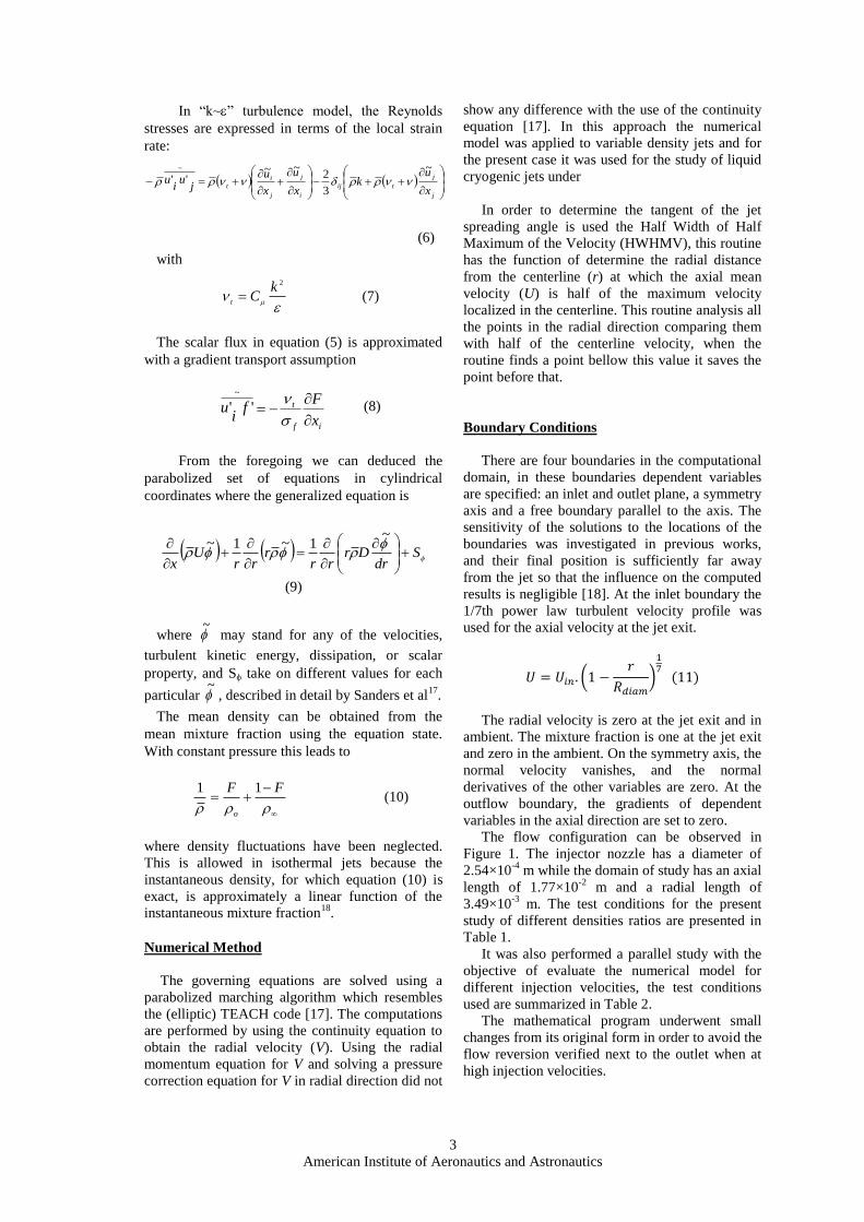
3
American Institute of Aeronautics and Astronautics
In “k~” turbulence model, the Reynolds
stresses are expressed in terms of the local strain
rate:
j
j
tij
i
j
j
it
x
uk
x
u
x
uj
ui
u~
3
2~~
''~
(6)
with
2kC
t (7)
The scalar flux in equation (5) is approximated
with a gradient transport assumption
if
t
x
Ff
iu
''
~
(8)
From the foregoing we can deduced the
parabolized set of equations in cylindrical
coordinates where the generalized equation is
S
dr
~
Drrr
~r
rr
~U
x
11
(9)
where ~
may stand for any of the velocities,
turbulent kinetic energy, dissipation, or scalar
property, and S take on different values for each
particular ~
, described in detail by Sanders et al17
.
The mean density can be obtained from the
mean mixture fraction using the equation state.
With constant pressure this leads to
FF
o
11 (10)
where density fluctuations have been neglected.
This is allowed in isothermal jets because the
instantaneous density, for which equation (10) is
exact, is approximately a linear function of the
instantaneous mixture fraction18
.
Numerical Method
The governing equations are solved using a
parabolized marching algorithm which resembles
the (elliptic) TEACH code [17]. The computations
are performed by using the continuity equation to
obtain the radial velocity (V). Using the radial
momentum equation for V and solving a pressure
correction equation for V in radial direction did not
show any difference with the use of the continuity
equation [17]. In this approach the numerical
model was applied to variable density jets and for
the present case it was used for the study of liquid
cryogenic jets under
In order to determine the tangent of the jet
spreading angle is used the Half Width of Half
Maximum of the Velocity (HWHMV), this routine
has the function of determine the radial distance
from the centerline (r) at which the axial mean
velocity (U) is half of the maximum velocity
localized in the centerline. This routine analysis all
the points in the radial direction comparing them
with half of the centerline velocity, when the
routine finds a point bellow this value it saves the
point before that.
Boundary Conditions
There are four boundaries in the computational
domain, in these boundaries dependent variables
are specified: an inlet and outlet plane, a symmetry
axis and a free boundary parallel to the axis. The
sensitivity of the solutions to the locations of the
boundaries was investigated in previous works,
and their final position is sufficiently far away
from the jet so that the influence on the computed
results is negligible [18]. At the inlet boundary the
1/7th power law turbulent velocity profile was
used for the axial velocity at the jet exit.
The radial velocity is zero at the jet exit and in
ambient. The mixture fraction is one at the jet exit
and zero in the ambient. On the symmetry axis, the
normal velocity vanishes, and the normal
derivatives of the other variables are zero. At the
outflow boundary, the gradients of dependent
variables in the axial direction are set to zero.
The flow configuration can be observed in
Figure 1. The injector nozzle has a diameter of
2.54×10⁻⁴
m while the domain of study has an axial
length of 1.77×10⁻²
m and a radial length of
3.49×10⁻³
m. The test conditions for the present
study of different densities ratios are presented in
Table 1.
It was also performed a parallel study with the
objective of evaluate the numerical model for
different injection velocities, the test conditions
used are summarized in Table 2.
The mathematical program underwent small
changes from its original form in order to avoid the
flow reversion verified next to the outlet when at
high injection velocities.

Table 5. Summary of test conditions
Case Pr Uin [m/s] Re T0 [K] ρ0
[Kg/m3]
ρ∞
[Kg/m3]
ω
1 0,583 3.0 72060 100 700 17,5 0,025
2 0,642 3.0 72060 100 700 24,5 0,035
3 0,825 3.0 72060 100 700 31,5 0,045
Table 6. Summary of test conditions for the injection velocity study
Case Pr Uin [m/s] Re T0 [K] ρ0
[Kg/m3]
ρ∞
[Kg/m3]
ω
4 0,583 3.0 72060 100 700 17,5 0,025
5 0,583 5.0 120100 100 700 17,5 0,025
6 0,583 10.0 240200 100 700 17,5 0,025
7 0,583 20.0 480400 100 700 17,5 0,025
Figure 1 – Flow Configuration
Results and discussion
In this section are presented the numerical
results obtained at the present work and compared
with the results exposed by Barata et al.18
. The
main objective is to extend the analysis performed
by Barata et al.18
to lower density ratios and then
compare them with the experimental data in order
to investigate the applicability of the variable
density approach to liquid jet injection into a
gaseous ambient under subcritical chamber
pressures but supercritical temperatures. The
parameter used to compare the numerical results
obtained in the present work with the results
exposed in Ref. 18 is the jet growth rate. The jet
growth rate is calculated by the tangent of the half
with of half maximum of the velocity (HWHMV),
this parameter is given by the calculation at each
axial point of the radial distance to the centerline at
which the axial velocity (U) is half of the velocity
at the centerline. However other parameters were
used in the characterization of the jet allowing also
some interesting conclusions and are shown in the
present paper.
Figures 2 and 3 show the typical velocity and
scalar fields of the jet for test conditions 1 (Figure
2) and 3 (Figure 3) of Table 1. In both cases the jet
structure is very similar, in the velocity field is
visible the appearance of the entrainment
phenomena close to the injector, with the jet fluid
dragging the ambient fluid. This phenomenon
causes the appearance of a vortex above the jet. It
appears that the position of the center of the vortex
is influenced by the density ratio, when the density
ratio increases the vortex center moves
downstream. The mixture fraction and density
scalar field show the rapid change of the jet
structure at the injector exit. The density scalar
field shows a faster decrease after the injector than
the mixture fraction scalar field. This suggests that

5
American Institute of Aeronautics and Astronautics
the density rapid decreased is not caused by the mixture of the injected fluid with the less dense
Figure 2 - Velocity and scalar fields of the jet with a density ratio of ω = 0.025 and a chamber
pressure of Pr = 0.583, (a) Velocity vectors, (b) Mixture fraction contours, (c) Density contours.

Figure 3 - Velocity and scalar fields of the jet with a density ratio of ω = 0.035 and a chamber
pressure of Pr = 0.642, (a) Velocity vectors, (b) Mixture fraction contours, (c) Density contours.

7
American Institute of Aeronautics and Astronautics
ambient fluid but indeed by a rapid expansion that
the injected fluid may experiences as it exits the
injector.
Figure 4 shows the axial variation of the
centerline density in a logarithmic scale for cases 1
to 3 of Table 1. It is visible that the centerline
density has a very similar behavior for the three
cases with a first stage of almost constant density
followed by a stage with a fast decrease of the
centerline density and then stabilization around the
ambient density value. A closer look to the graphic
allows however to perceive that the case with a
higher ambient pressure has a slightly higher
decrease rate which is in agreement with the
density scalar field observed in Figures 2 and 3.
The length of the potential core based on the
density is defined by the initial, almost constant,
stage of the axial variation of the centerline density
which lasts until an approximately length of X/D =
3 diameters for the three studied cases.
Figure 4 – Axial variation of the centerline
density.
The centerline velocity decay is shown in
Figure 5 for the cases 1, 2 and 3. The velocity
decay has a similar profile for the three cases with
a first stage with almost no decay followed by a
stage with a higher rate of decay and finally a
stabilization like observed in Figure 4 for the
variation of density. A higher rate of velocity
decay is observed for the cases with higher
ambient pressure indicating a greater interaction
between the injection and ambient fluids. The
length of the potential core based on the velocity
decay is defined in the present work by the axial
distance to the injector at which the centerline
velocity has decayed 10%. The length of the
potential core is between X/D = 7.9 and X/D =
7.47 diameters respectively for cases 1 and 3. Thus
it is verified that the length of the potential core
based on centerline velocity decay has a
substantially different value that the approximately
X/D = 3 diameters found for the potential core
based on the centerline density. This is an
interesting result, as in previous works the length
of the potential core based on the density has
approximately the same value as the one based on
the velocity decay, and hypothesizes that the
injected, possibly identify by the observation of
the scalar fields, may contribute with kinetic
energy to the jet.
Figure 5 – Centerline velocity decay.
Figure 6 shows the half width of the half
maximum of the velocity (HWHMV) for the cases
1, 2 and 3 of Table 1. The three cases have a
similar evolution of the HWHMV across the
domain of study with an almost linear first stage
and a second non linear stage. The tangent of the
slope of the almost linear stage corresponds to the
jet growing rate. Observing the graphic it is
possible to conclude that the jet growing rate is
very similar for the three studied cases with only a
slightly decrease as the chamber pressure
increases. This was however not an expected result
as in several previous work the increase of the
chamber pressure causes an increase in the jet
growing rate.
In Figure 7 are shown the decay rates of
velocity and density after the potential core for the
cases of Table 1. For both velocity and density an
increase in the injection chamber pressure has as
result an increase of the decay rate which is in
agreement with previous works from other authors,
however this effect is more pronounced in the
velocity decay. The velocity also shows for the
three cases a higher decay rate then the density
although is important to remember that the density

decay starts earlier then the velocity decay due to
the longer potential core obtained for the velocity.
Figure 6 – Half width of half maximum of the velocity.
Figure 7 – Decay rate of the centerline velocity and density.

9
American Institute of Aeronautics and Astronautics
Figure 8 - Tangent of the spreading angle versus the chamber-to-injectant density ratio and
representation if limit of applicability of the Variable Density approach.
Figure 8 is similar to the graphic presented by
Barata et al.18
and shows the tangent of the jet
spreading angle, calculated by the half width of
half maximum of the velocity, in order to the
density ratio. In addition to the three cases of Table
1 the graphic contains also results obtained by
other authors in previous investigations including
the results of Barata et al.18
, the investigation
which the present work pretends to extend. The
results achieved in the present work are
represented in red while those achieved by other
authors are represented in black. Obversing the
graphic it is visible that the result obtained for a
density ratio of ω = 0.025 agree very well with the
experimental result obtained by Chehroudi et al.23
,
the result obtained for a density ω = 0.035 is in
total agreement with the modeling results of the
same author. The ω = 0.045 density ratio case
shows a slight divergence from previous result but
is still very close to the modeling result of
Chehroudi et al.23
. The test of the present variable
density approach to lower density ratios, which are
not presented here, allow the conclusion that the
density ratio of ω = 0.025 is the lowest value liable
to be modeled by the present mathematical model.
This conclusion is represented in Figure 8 by the
vertical red line that marks the limit of
applicability of the variable density approach.
The influence of the injection velocity in jet
behavior was also subject of analysis at the present
investigation. The objective was to perform a
better characterization of the mathematical model.
In order to achieve this objective the variable
density approach was tested for different injection
velocities as presented in Table 2.
Figure 9 shows the velocity and scalar fields for
the test case 7 of Table 2. It is visible that the jet
has the same structure found in Figure 2
corresponding to the case 4 of Table 2. It’s
however possible to verify that the vortex center
appears in localization further downstream, also
the mixture fraction and density show a slower
evolution across the centerline when compared
with the case with slower injection velocity. The
axial variation of the centerline density shown in
Figure 10 corroborates the observation stated

Figure 9 - Velocity and scalar fields of the jet with a density ratio of ω = 0.025 and an injection velocity of Uin
= 20 m.s-1, (a) Velocity vectors, (b) Mixture fraction contours, (c) Density contours.

11
American Institute of Aeronautics and Astronautics
above. The centerline density shows a slower
decrease for higher injection velocities. One
interesting observation is the increase of the
potential core based on density as the injection
velocity increases. Similar observations are made
for the centerline velocity decay. As the injection
velocity increases the potential core based on the
velocity decay increases and the centerline velocity
shows a lower rate of decay, this is somehow
contrary to the expected since an increase in the
injection velocity should lead to an increase of
drag forces between the injected and the ambient
fluid and this way increase the velocity decay rate.
Like in the axial variation of the centerline also for
the centerline velocity decay the case 5 with an
injection velocity of Uin = 5 m.s-1
shows a behavior
different from the tendency followed by the other
three cases.
Figure 10 - Axial variation of the centerline density
for the cases 4, 5, 6 and 7 of the Table 2.
Figure 11 - Centerline velocity decay for the cases 4,
5, 6 and 7 of the Table 2.
The half width of half maximum of the velocity
is shown in Figure 11. Again the case 4 of Table 2
shows a different HWHMV structure then the
other three cases not having an almost linear stage.
By the observation of the graphic can be concluded
that an increase of the injection velocity causes a
decrease in the jet spreading angle.
Figure 12 - Half width of half maximum of the
velocity for the cases 4, 5, 6 and 7 of the Table 2.
Conclusions
Barata et al. [18] had concluded that the
variable density mathematical model could be
successfully used in the study of cryogenic jets
injected initially at subcritical temperatures into an
environment at a supercritical temperature over a
range of subcritical and supercritical pressures
[18]. The objective of the present work was to
extend the study performed by Barata et al. [18] to
lower chamber-to-injection fluid density ratios.
Like in Barata et al. [18], for this investigation an
injection of cryogenic liquid nitrogen into a
gaseous nitrogen environment was simulated.
In the analysis of the obtained result were
identified some interesting new results. The fastest
mixture fraction scalar field evolution when
compared with the density scalar field together
with the difference between the potential core
based on density and the one based on velocity
decay, suggests that a vigorous expansion of the
injected fluid happens as it enters the injection
chamber. And the longer potential core based on
the velocity decay indicated that expansion may
somehow contribute with kinetic energy to the jet.
The results of the half with of half maximum of
the velocity allowed the determination of the jet
growth rate with are in general agreement with the
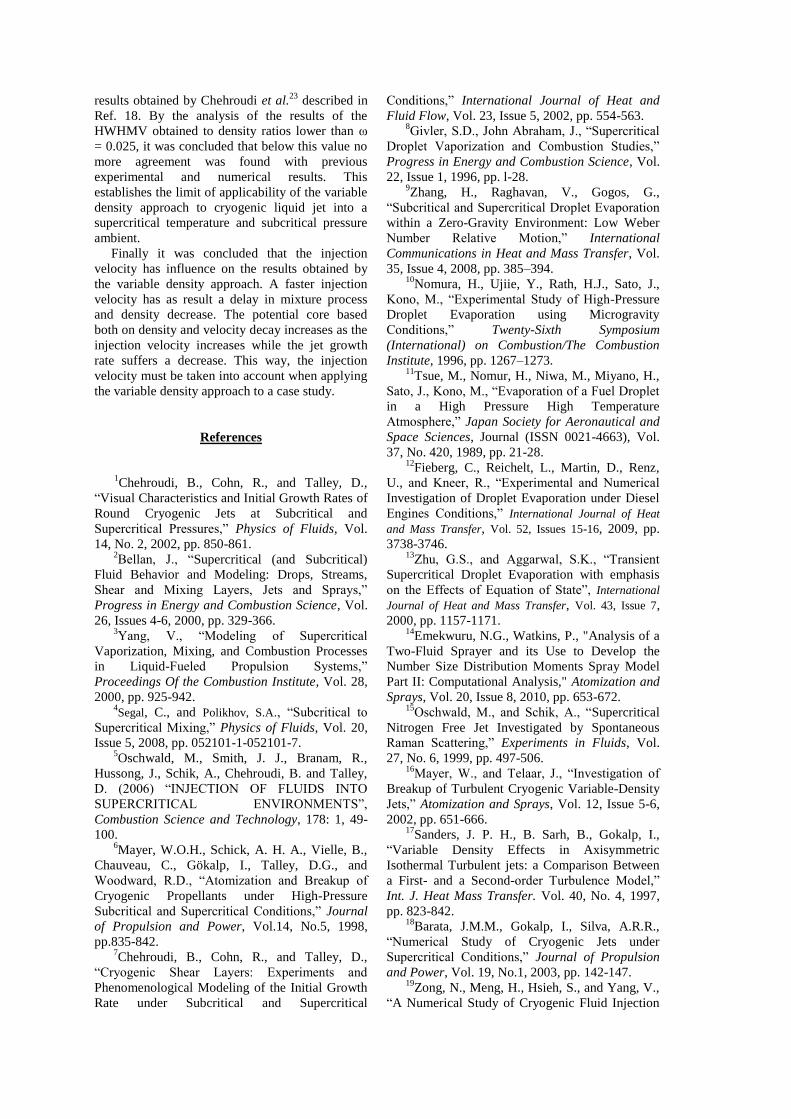
results obtained by Chehroudi et al.23
described in
Ref. 18. By the analysis of the results of the
HWHMV obtained to density ratios lower than ω
= 0.025, it was concluded that below this value no
more agreement was found with previous
experimental and numerical results. This
establishes the limit of applicability of the variable
density approach to cryogenic liquid jet into a
supercritical temperature and subcritical pressure
ambient.
Finally it was concluded that the injection
velocity has influence on the results obtained by
the variable density approach. A faster injection
velocity has as result a delay in mixture process
and density decrease. The potential core based
both on density and velocity decay increases as the
injection velocity increases while the jet growth
rate suffers a decrease. This way, the injection
velocity must be taken into account when applying
the variable density approach to a case study.
References
1Chehroudi, B., Cohn, R., and Talley, D.,
“Visual Characteristics and Initial Growth Rates of
Round Cryogenic Jets at Subcritical and
Supercritical Pressures,” Physics of Fluids, Vol.
14, No. 2, 2002, pp. 850-861. 2Bellan, J., “Supercritical (and Subcritical)
Fluid Behavior and Modeling: Drops, Streams,
Shear and Mixing Layers, Jets and Sprays,”
Progress in Energy and Combustion Science, Vol.
26, Issues 4-6, 2000, pp. 329-366. 3Yang, V., “Modeling of Supercritical
Vaporization, Mixing, and Combustion Processes
in Liquid-Fueled Propulsion Systems,”
Proceedings Of the Combustion Institute, Vol. 28,
2000, pp. 925-942. 4Segal, C., and Polikhov, S.A., “Subcritical to
Supercritical Mixing,” Physics of Fluids, Vol. 20,
Issue 5, 2008, pp. 052101-1-052101-7. 5Oschwald, M., Smith, J. J., Branam, R.,
Hussong, J., Schik, A., Chehroudi, B. and Talley,
D. (2006) “INJECTION OF FLUIDS INTO
SUPERCRITICAL ENVIRONMENTS”,
Combustion Science and Technology, 178: 1, 49-
100. 6Mayer, W.O.H., Schick, A. H. A., Vielle, B.,
Chauveau, C., Gökalp, I., Talley, D.G., and
Woodward, R.D., “Atomization and Breakup of
Cryogenic Propellants under High-Pressure
Subcritical and Supercritical Conditions,” Journal
of Propulsion and Power, Vol.14, No.5, 1998,
pp.835-842. 7Chehroudi, B., Cohn, R., and Talley, D.,
“Cryogenic Shear Layers: Experiments and
Phenomenological Modeling of the Initial Growth
Rate under Subcritical and Supercritical
Conditions,” International Journal of Heat and
Fluid Flow, Vol. 23, Issue 5, 2002, pp. 554-563. 8Givler, S.D., John Abraham, J., “Supercritical
Droplet Vaporization and Combustion Studies,”
Progress in Energy and Combustion Science, Vol.
22, Issue 1, 1996, pp. l-28. 9Zhang, H., Raghavan, V., Gogos, G.,
“Subcritical and Supercritical Droplet Evaporation
within a Zero-Gravity Environment: Low Weber
Number Relative Motion,” International
Communications in Heat and Mass Transfer, Vol.
35, Issue 4, 2008, pp. 385–394. 10
Nomura, H., Ujiie, Y., Rath, H.J., Sato, J.,
Kono, M., “Experimental Study of High-Pressure
Droplet Evaporation using Microgravity
Conditions,” Twenty-Sixth Symposium
(International) on Combustion/The Combustion
Institute, 1996, pp. 1267–1273. 11
Tsue, M., Nomur, H., Niwa, M., Miyano, H.,
Sato, J., Kono, M., “Evaporation of a Fuel Droplet
in a High Pressure High Temperature
Atmosphere,” Japan Society for Aeronautical and
Space Sciences, Journal (ISSN 0021-4663), Vol.
37, No. 420, 1989, pp. 21-28. 12
Fieberg, C., Reichelt, L., Martin, D., Renz,
U., and Kneer, R., “Experimental and Numerical
Investigation of Droplet Evaporation under Diesel
Engines Conditions,” International Journal of Heat
and Mass Transfer, Vol. 52, Issues 15-16, 2009, pp.
3738-3746.
13Zhu, G.S., and Aggarwal, S.K., “Transient
Supercritical Droplet Evaporation with emphasis
on the Effects of Equation of State”, International
Journal of Heat and Mass Transfer, Vol. 43, Issue 7,
2000, pp. 1157-1171.
14Emekwuru, N.G., Watkins, P., "Analysis of a
Two-Fluid Sprayer and its Use to Develop the
Number Size Distribution Moments Spray Model
Part II: Computational Analysis," Atomization and
Sprays, Vol. 20, Issue 8, 2010, pp. 653-672.
15Oschwald, M., and Schik, A., “Supercritical
Nitrogen Free Jet Investigated by Spontaneous
Raman Scattering,” Experiments in Fluids, Vol.
27, No. 6, 1999, pp. 497-506.
16Mayer, W., and Telaar, J., “Investigation of
Breakup of Turbulent Cryogenic Variable-Density
Jets,” Atomization and Sprays, Vol. 12, Issue 5-6,
2002, pp. 651-666.
17Sanders, J. P. H., B. Sarh, B., Gokalp, I.,
“Variable Density Effects in Axisymmetric
Isothermal Turbulent jets: a Comparison Between
a First- and a Second-order Turbulence Model,”
Int. J. Heat Mass Transfer. Vol. 40, No. 4, 1997,
pp. 823-842.
18Barata, J.M.M., Gokalp, I., Silva, A.R.R.,
“Numerical Study of Cryogenic Jets under
Supercritical Conditions,” Journal of Propulsion
and Power, Vol. 19, No.1, 2003, pp. 142-147. 19
Zong, N., Meng, H., Hsieh, S., and Yang, V.,
“A Numerical Study of Cryogenic Fluid Injection
13
American Institute of Aeronautics and Astronautics
and Mixing under Supercritical Conditions,”
Physics of Fluids, Vol. 16, No. 12, 2004, pp. 4248-
4261. 20
Sierra-Pallares, J., Parra-Santos, M.T.,
García-Serna, J., Castro, F., Cocero, M.J.,
“Numerical Analysis of High-pressure Fluid Jets:
Application to RTD Prediction in Supercritical
Reactors”, Journal of Supercritical Fluids, Vol.
49, 2009, pp. 249-255. 21
Schmitt, T., Selle, L., Cuenot, B., and
Poinsot, T., “Large-Eddy Simulation of
Transcritical Flows”, Comptes Rendus Mécanique,
Vol. 337, Issues 6-7, June-July 2009, pp. 528-538. 22
Kim, T., Kim, Y., Kim, S., “Numerical study
of cryogenic liquid nitrogen jets at supercritical
pressures,” The Journal of Supercritical Fluids,
Vol. 56, Issue 2, 2011, pp. 152-163. 23
Chehroudi, B., Cohn, R., and Talley, D.,
“Spray/Gas Behaviour of Cryogenic Fluids under
Sub- and Supercritical Conditions”, Eighth
International Conference on Liquid Atomization &
Sprays Systems, ICLASS-2000, Pasadena,
California, USA, July 16-20, 2000.