Evaluation of joint probability density function models ... · Evaluation of joint probability...

Center for 7"urbulence ResearchProceedings o/ the Summer Program 1996

167

Evaluation of joint probability densityfunction models for turbulent nonpremixed

combustion with complex chemistry

By N. S. A. Smith 1, S. M. Frolov 2 AND C. T. Bowman :_

Two types of mixing sub-models are evaluated in connecti()n with a joint-scalar

probability density flmction method for turbulent nonprenfixed combustion. M()(lcl

calculations are lnade and compared to simulation resuhs for homogeneously dis-

tributed methane-air reaction zones, mixing and reacting in decaying turbulence

within a two-dimensional enclosed domain. The comparison is arranged to ensure

that both the simulation and model calculations a) make use of exactly the same

chemical mechanism, b) do not involve non-unity Lewis number transport of species,

and c) are free from radiation loss. The modified Cm'l mixing sub-model was found

to provide sut)erior predictive accuracy over the simple relaxation-to-mean sub-

model in the case studied. Accuracy to within 10 - 20% was found for global means

of major species and temperature; however, nitric oxide prediction accuracy was

lower and highly det)endent on the choice of mixing sub-model. Both mixing sub-

models were found to produce non-t)hysical mixing behavior for mixture fractions

removed from the immediate reaction zone. A suggestion for a further modified

Curl mixing sub-model is made in connection with earlier work done in the field.

1. Introduction

A large number of practical combustion systems can |)e said to operate in a

nonpremixed turbulent regime. Under these conditions, tirol and oxidizer react

concurrently as they are mixed together through the cascade of scales from turbulent

stirring down to molecular diffusion. The nont)remixed mode of combustion is

distinct from the premixed mode in that the propagation of reaction fronts through

a flammable mixture is not encountered. This is by virtue of the concurrence of

mixing of reactants to a flammable state, and reaction.

When put in the context of the partially premixed flame studies discussed else-

where in this volume, nonpremixed combustion refers to all the t)henomena that

occurs after the passage of any initial igniting flame fronts. The bulk of chemical

activity in gas turbine combustors, compression ignition internal combustion en-

gines, and a great many other classes of devices, occurs downstream of stabilizing

flow structures in a purely nonpremixed mode.

1 Center for Turbulence Research

2 N. N. Semenov Institute for Chemical Physics, Moscow, Russia

3 Stanford University

https://ntrs.nasa.gov/search.jsp?R=19970014662 2020-01-16T21:25:39+00:00Z

168 N. S. A. Smith, S. M. Frolov _t C. T. Bowman

The critical design issues facing gas turbine combustor and diesel engine designers

at present center on reducing pollutant formation in order to meet present and

future emission regulations. In order to understand and be able to predict the

occurrence of unwanted byproducts, such as oxides of nitrogen (NOx) and soot,

it is essential that allowances be made for the interactions which occur between

finite rate chemical reactions and turbulent mixing processes. Nitric oxide (NO) is

a species whose formation in flames is limited by chemical kinetic rates which are

slow in comparison to typical mixing rates, and thus cmmot be adequately predicted

using a model assulnption of mixing-limited chemistry.

Many methods have boon proposed which seek to accurately predict the inter-

action of finite rate chomistry and turbulent mixing. One of the most promising

groups is the Joint Probability Density Function (JPDF) methods as employed by

Pope (1981, 1985, 1990) and others (see Chen & Kolhnann 1988, 1992, 1994). Thevariants of the JPDF lnethod have been used to successfully predict nitric oxide

h)rmation in turbulent jet diffusion flames of hydrogen (Chen & Kollmann 1992,

Chen et al. 1995, Smith ct al. 1993). The effectiveness of the JPDF model in these

experimental comparisons for hydrogen and other tvsts involving hydrocarbon fuels

(Chen 1996) make it a prime candidate for incorporation in design tools for use

with more practical combustion systems.

Correa and Pope (1992) have already begun to take steps towards implement-

ing JPDF inethods in a computational framework Inore suited to practical calcula-

tions. They showed reasonable agreexnent between the predictions of a hybrid JPDF

method in an elliptic flow solver, with experimental data gathered behind a bluff

body stabilized flame. One difficulty with the experimental comparison of Correa

and Pope (1992) and those of the jet flame experiments described above is that

there are a number of other models and approximations that nmst be incorporated

in order to produce usefill predictions, but these other models make it difficult to

ascertain the inhorent accuracy of the JPDF method.

Where only a .scalar JPDF method is employed (as in the studies cited), a tur-

bulence model must be used to solve for the turbulent flow field. In the jet flame

studies, radiation modeling can be problematic (Smith et al. 1993, 1996) and thus

make it difficult to evaluate the performance of the JPDF model directly. Further,

since the JPDF model cmmot be easily employed with large chemical reaction mech-

anisms, due to conlputational constraints, it is often necessary to employ reduced

chemical descriptions of the filll reaction set. This modeled ahbreviation of a chem-

ical system also introduces uncertainty when comparing with physical experiments.

Extraneous modeling issues can be swept aside if direct numerical simulation

(DNS) is used as an evaluation tool. With DNS it is possible to construct an

idealized numerical experiment where unwanted physical effects can be excluded by

design. For the case of mixing and reaction of filel and oxidizer pockets in decaying

isotropic turbulence, the flow field is at its simplest, radiation losses can be dropped

from consideration, and connnonality between the modeled and simulated chemical

reaction schemes can be (,nsured.

The purpose of this study was to compare JPDF model predictions with DNS

PDF modcl_ for turbulent combu._tion 169

observations for the nonpremixed combustion of methane and air in decaying tur-

bulence. Tile chemical mechanisnl employed in both the DNS and in the JPDF

model calculations included prompt and thermal NO fl)rmation pathways and so

allowed an evaluation of the model's NO prediction capabilities to be made.

2. Joint scalar PDF equations

Given a chemical system of N species it. is possible to construct a chemical coml)o-

sition vector, where each coordinate correst)onds to a possible species mass fraction.

It is then possible to define the probability F that t h(, instantaneous compositi()n

vector at a tinle t at a sample point is in the immediate vicinity of _/._2"

F(_'l ..... _/'x:t) -- Prob{_?l < 01 __ t/'l 4-dl./!'l,... ,t/'N _. ON _ _!"._' JFd(_"N} (1)

The density-weighted joint scalar I)robability density flmction, J:, in composition

space is then defined as the partial derivative with respect to the sl)ecies dimensions.

](_'1,-.. _'._') = O(_:''l .... '_%') O"F (2)' < p > 0¢1...00N

For homogeneous flows, the evolution of the joint scalar PDF is then given by the

following (see Chen and Kollnmnn 1994), where 01,- is the instantaneous reaction

rate of the kth species at time 1, and \k.l is the joint scalar dissipation rate for the

kt.h and/th species.

+ ((_k])- OCztOc)t(\t,,/) (3)

The influence of chemical reactions on the temporal evolution of the joint scalar

PDF is similar to a convective velocity field in composition space. Dissit)ation

of scalar fluctuations through mixing, as represented by the second right hand

side term, lead to reductions in the variances and covariances of the species and a

sharpening of the joint PDF at the mean composition.

As chemical systems of practical interest can have an extremely large number of

important species, the dimensionality of the joint PDF can also be large. Stochastic

methods recommend themselves as the solution method of choice in these cases

(Pope 1981 ).In a Monte Carlo approach, a large number of stochastic particles are operated

upon by model processes in a Lagrangian frame of reference. The model processes

are designed in such a way as to cause the joint PDF of all the particles to behave

according to the evolution equation above.

Each stochastic particle has a definite location in composition space at any given

time. The evolution of the ith chemical component of the jth stochastic particle

can be expressed in terms of a chemical reaction source term, 0i, and molecular

mixing term, ri_, as given below.

170 N. S. A. Smith, S. M. Frolov _t C. T. Bowman

-_ = Q, + m i (4)

A significant advantage of the JPDF method over other models is that the chem-

ical source terms Q_ can be evaluated exactly without need for a model. The

difl:iculty with the Lagrangian formulation lies with the treatment of tile molecular

mixing terms _h_.

2. I Molecular mixing models

A wide variety of molecular mixing models have been prot)osed for 7h i in the

past (see Pope 1981, Chen and Kollmann 1994). The simplest useful model is a

deterministic relaxation-to-the-mean (RTM) expression as given below, where _'

denotes a turbulent mixing frequency.

¢, > (5)

The deterministic RTM model has the advantage of being simple to implement

within a complex practical calculation and allows the mixing and reaction terms of

the stochastic equations to t)e solved simultaneously. All particles are operated on

by both the molecular mixing and reaction models at all stages of tile computation.

A disadvantage of the RTM model is that it does not predict the correct mixing

behavior of two fluids in an isotropically decaying turbulent field. Instead of causing

a mixture fraction PDF to tend towards a Gaussian distribution with increasingtime. the RTM model allows the flatness of the PDF to increase without bound.

More sophisticated mixing models have been derive(l from the Curl coalescence-

dispersion models for droplet, mixing. Vv'hereas the original Curl mixing model gives

rise to discontinuous joint PDFs, the modified Curl model proposed t)y Janicka et

al. (1979), and Dopazo (1979), yields the desired continuous joint PDFs. Mixing

is modeled by ot)erating on a small number of particles at each time step of the

calculation. Particle pairs are chosen at random from the comt)lete particle ensem-

ble, and are caused to mix with one another to a randomly varying degree a. The

resultant comt)ositions of the jth and/cth particle after mixing interaction are given

by the following.

_*= a¢_ + ._(i- a)(_ + 0_) (6)

1 jO_* = a¢_ + _(1 - a)(O)' + 0,) (7)

The number of random particle pair selections that must be made per timestep

of the calculation is given by the following (see Pope 1982), where B is a con-

stant number that depends on the pair selection scheme, and _(_t is the timestep

nondimensionalized by the mixing frequency.

PDF rnodeI._ for t'tLrb'ulent combustion 171

Tile use of ran(lonl particle interaction (tlPI) models provides a framework for

the implementation of schemes that reflect more of the physical nature of mixing.

An example of the benefit that can be derived from RPI models can be found in

the "particle age" modification suggested by Pope (1982). This model can be tuned

to enforce asymptotic Gaussianity on conserved scalar PDFs in decaying isotropicturbulence.

One potential drawback incurred in using particle interaction models is that the

mixing process can then no longer be solved simultaneously with the chemical re-

action process. The two processes nmst be decoupled, and this can cause problems

where the rates of mixing and reaction are both very large relative to the inverse

of the timestep. Such problems are likely to occur when combustion occurs in the

flamelet regime (see Anand & Pope 1987).

Both the RPI model and the simple RTM model were employed in JPDF cal-

culations against the DNS data. The results of this comparison are presented inSection 4.

3. Simulation conditions

Due to resource and time constraints, the direct numerical simulation was limited

to a two-dimensional calculation of nonpremixed combustion in a decaying turbulentfield.

As the JPDF method is inherently statistical in nature, it was desirable to max-

imize the number of DNS data points in the domain that could be included in a

single statistical set. To this end, the simulation was performed with an initially

isotropic turbulent velocity field and distribution of fltel and oxidizer pockets. The

initial distril)ution of chenfical species was determined from a phase scrmnbled E -k

spectrum for a conserved scalar, known as mixture fraction _ (see Fig. 1).

Mixture fraction is a normalized scalar that is equal to unity where all of the

local has mass originated from the nominal fuel source, irrespective of its reacted

state, and zero where all the local mass has originated from the oxidizer source.

Given the distribution of the conserved scalar, mixture fraction ({), reactive scalar

profiles were mapped onto the domain according to adiabatic equilibrium profiles

in mixture fraction space (see Fig. 2).

Zones on the domain with a stoichiometric mixture fraction (_ = 0.055) were thus

assigned a species and temperature composition corresponding to adiabatic equi-

librium conditions at stoichiometric. Domain regions with higher or lower mixture

fraction values were given correspondingly richer or leaner blends of equilibratedfluid.

Note that the richest mixture fraction allowed in the initialization of the simula-

tion domain was < { >= 0.18. This mixture fraction is beyond the rich flammabil-

it 3, limit of methane-air mixtures at standard temperature and pressure. Of all the

species present in the simulation, only nitric oxide (NO) was initialized as beingzero at. all mixture fractions.

By initializing the simulation using the method described above, the flame zones

were effectiw,ly ignited simultaneously, albeit artificially, prior to run t.ime. This

172 N. S. A. Smith, S. M. Frolov _J C. T. Bowman

Y

x

FIGURE 1. Initial distribution of the conserved scalar. Dark regions denote fuel

rich zones ( = 1 while light regions denote fuel lean zones _ = 0.

0.25

i,_ 0.15-

°'tr_ 005(J]

/

//

0 0.0_ 0.1 0.15

Mixture fraction

FIGURE 2. Adiabatic equilibrium species mass fraction profiles in mixture fraction

space. Symbol key : + - O2, x - CO, o - COz, /X - H20.

was done to avoid a potentially long transient period where (presumably) triple

flames would propagate along the unburnt flammable ribbons between the fuel and

oxidizer pockets away from the ignition points.

In order to avoid the establishment of intense pressure waves as a result of map-

ping flame zone temperatures onto an initial cold flow field, the local densities were

adjusted everywhere to maintain a uniform initial pressure field. The existence

of large density gradients after initialization caused a short period where the flow

field reorganized to preserve continuity. It is difficult to draw a parallel in behavior

between the decay of turbulent motions in the reacting case and the well known

trends in inert grid turbulence. The former case is subject to dilatation, variable

PDF models for turbulent combustion 173

FIGURE 3.

c¢

1.l

0.2

Pressure [atm] ,

0 00014 000279

Time (msec)

Variation in sinmlated global mean quantities with calculation time.

viscosity, and baroclinic torque effects that are absent in the latter.

Unfortunately, it was further found that it was not possible to perform simulations

with a combination of periodic boundary conditions and the initialization technique

described above. No satisfactory explanation for this restriction has been found.

It was found, however, that the calculation could proceed without hindrance if the

domain was instead bounded by adiabatic slip walls encompassing a small filter

zone with initially damped wall-normal velocity.

Under the sinmlation conditions described above, the flow and mixing fields on a

central portion of the grid (2102 ) were found to be statistically homogeneous. All

of these points were then used in each of the statistical samples taken periodically

throughout the temporal evolution of the simulation. With the passage of time, tur-

bulent motions caused parcels of fllel and oxidizer to be convected into close prox-

imity while molecular diffusion fed the reaction zones present at the fuel/oxidizerinterfaces.

Unmixedness, U, is defined here as the global variance of mixture fraction nor-

realized by the maximum possible variance, which is given by the product of the

differences between the global mean and the maximum and mininmm possible val-

ues of conserved scalar. Unmixedness is thus equal to unity when no mixed fluid is

present, and zero when all fluid has been mixed to a uniform state. The gradual de-

cay in the unmixedness of the conserved scalar is plotted along with nondimensional

scalar dissipation rate and mean pressure in Fig. 3.

It is evident that the molecular mixing processes promoted by turbulent stirring

rapidly mixed the conserved scalar tmvards uniformity, but that at the end of the

simulation the unmixedness was still substantial at approximately U = 0.3. As a

result of the increase in the characteristic turbulent time scale and the decrease in

local conserved scalar gradients, the scalar dissipation rate can be seen to decreasewith time.

The simulation was carried out using a Fickian assumption for the molecular

174 N. S. A. Smith, S. M. Frolov _'4 C. T. Bourne, an

transport of the species, as traces, in a background gas (N2). All st)ecies were

assigned uniform Lewis Immbers of unity in order to allow a fair conll)arison with

the JPDF model predictions. The JPDF model is not strictly valid where significant

differential nloleeular diffusion between the species is present.

As the reactions proceeded, more and more fuel and oxidizer were consumed and

progressively more sensible enthalpy was released int() the system. The release of

heat in the confined systenl caused the mean t)ressure in the domain to double over

the course of the simulati(m (see Fig. 3). The change in global mean si)ecics Inass

fl'actions during the course of the sinmlation can be seen in Fig. 4.

FIGURE 4.

lation time.

,..b-,0 055. "-

o ooo_4 o ,oo_7._

Time (msec)

Variation in simulated glol)al mean species mass fi'actions with calcn-

The turbulent Reynolds number determined use ()f the mean molecular viscosity

(recall that the local temperature variations giw' rise to a seven-fold variation in

local dynamic viscosity) slowly from approxinmtely 30 down to 20 over the durationof the simulation.

The simulation conditions correspond physically t() a small area of intensely mixed

fluid of the order of 3 millimeters on each side. In some ways the sinmlation con-

ditions may be analogous to the kind of conditions experienced inside high power-

density combustion devices of practical interest. The DNS (lomaill might be thought

of as representing a single computational cell in a much larger grid used in a prac-tical model calculation. In this sense it is of some interest to observe how well the

JPDF model performs in this single cell, as it could well haw' implications for use

of the model in a large nmhi-cellular calculation.

With the assumption of isotropy, the JPDF model reduces to a (limensionaliy

degenerate case devoid of mean gradients. The case is similar to those studied

by Correa (1993) an(1 Chen (1993), except that it is unsteady, whereas the earlier

studies were for stead)' combustion.


g.1 Chemical reaction mechanism

An eight step reduced chemical mechanism for methane combustion was provided

by Frolov (1996) for use in both the DNS and JPDF calculations. The mechanism

consists of global steps which do not make explicit use of any radical species, such as

hydroxyl (OH), methyl (CH3), and so on, but instead employs tuning factors for thefuel oxidation and prompt NO_ steps. These tuning factors are incorporated into

the pre-exponential coefficients in the Arrhenius expressions and make allowance for

variations in local equivalence ratio, fuel species, and pressure. The tuning constants

were derived by Frolov (1996) from comparison of the reduced mechanism with fullmechanism calculations in counterflow laminar premixed flames.

CH4 + 1.502 _ CO + 2H20

CO + H20 _ C02 + H2

C02 + H2 _ CO + 1t20

2H2 + 02 _ 2H20

2C0 + 02 _ 2C02

CH4 + 02 + N2 _ CH4 + 2NO

N2 + 02 _ 2NO

NO + NO _ N2 + 02

(I)

(IIf)

(IIb)

(III)

(IV)

(v)

(VIf)

(VIb)

The Arrhenius rate constants corresponding to the above reaction steps are given

below where Ai, ni and Ei denote the pre-exponential factor, temperature index,

and activation energy for reaction number i, and p is the local pressure in bar.

No. Ai( mol, L, s) ni Ei( kcal /mol)

I A1/p 0.0 50.0

IIf 1.0 x 1012/p 0.0 41.5IIb 3.1 x 1013/p 0.0 49.1

III 7.0 x 1013/p 2 0.0 21.0

IV 8.5 x 1012/p 2 0.0 21.0

V A_/p 2 0.0 50.0VIf 1.7 x 1017 -0.5 136.0VIb 4.1 x 10a_ -0.5 93.3

The pre-exponential factors for reactions I and V are functions of the local equiv-

alence ratio/3. Frolov (1996) determined the appropriate values of A1 and A5 at

a range of equivalence ratios from/3 = 0.67 up to /3 = 1.54. The pre-exponentialfactors vary nonlinearly over the range such that the lean limit values are orders

of magnitude greater than the rich limit values. The values under stoichiometricconditions for each is A1 = 2.57 x 1015L/(mol •s) and As = 7.03 x 1013L2/(mo12s).

176 N. S. A. Smith, S. M. Frolov _'4 C T. Bowman

At the suggestion of Frolov (1996), linear interpolation between the known values

for Al and A5 was used to determine values for intermediate mixing states.

At this stage there are some questions as to the a('cm'acy of the chemical mech-

anism described above, since it appears to give quantitatively inaccurate values

for unstrained laminar flame speed and extinction strain rate. However, as both

the DNS and JPDF computations employed the same chemical mechanism, the

quantitatiw, accuracy of the mechanism is not an issue in comparing one with theother.

4. Comparison of predictions and simulation data

The JPDF model calculations were in each cas(, initializ(,d directly from the (l()-

main of the DNS data base. Each of the' 2,000 st_wlmstic particles used in the

model were assigned compositions selected at random from the domain. Special

care was taken to ensure that the initial t)article distribution in composition space

gave rise to the same statistics as was found in th_ simulation. As the partich_s

used in the model were of equal mass, this required that ttl(' mnnber of potential

particle assignments for each domain cell be proportional to the local fluid density.

An assignment table was constructed for the purl)oS¢ of partich, initialization,

where there was an equal probability of a particle b_'ing; assigned the' composition

of any entry in the table. The ntmlber and compositi(m of the table entries was

determined from the' sinmlation domain, such that a v,_ry h_w density cell would

only provide a single entry whereas a high density c_'ll would provide a number of

repeated entries, each with the same composition as the originating cell. As the

central portion of the simulation domain consisted of approxinmtely 45,000 cells

and the ratio of the mean cell density to the Ininimum cell density was of order

2 - 3, this gawr rise to a table containing around 10(I, (}00 entries. Of that IlUlllber,

2,000 were selected at random, without replacement, for particle assigmnent.

Model calculations were then allowed to proceed according to Eq. 3, with a

revised m_,an pressure calculated after every time st,'p. Mixing time scah.s weredrawn fl'om the DNS for use in the model calculation.

_.1 Global mean behavior

Global mean species yMds and pressure were predicted using 1RTM and RPI

mixing sub-models (see Section 2.1) within the .IPDF model.

Typical model predictions for mean pressure, initializ_'d fi'om the initial DNS

data, are plotted in comparison with the DNS pressure record in Fig. 5. The I/TM

prediction displays too slow an initial pressure rise, indicating a too modest sensible

energy release rate. Towards the end of the sinmlati_m period, the RTM-modeled

mean pressure rises at a rate greater than that seen in the DNS.

The random particle interaction model prediction tends to lie substantially closer

to the DNS curve than do the predictions of the RTM model. At its worst the 12TM

model exhibits an approximate 20% discrepancy below the' DNS curve, while the

1qPI model exhibits a maximum underprediction on the order of 10_,.

The model predictions fi)r mean carbon dioxide (CO,) mass fl'action forlnation

reflect the predicted mean pressure behavior (see Fig. 61. Carbon dioxide is one of


2e+05

_._ 1.5e+05

le+'O_

0.0007 0_0014 0.0021 0,0028

FIGURE 5. Comparison of simulated and predicted mean pressure rise. chemical

description of H2/N2-_fir combustion. Symbol key : + - JPDF-RTM, x - JPDF-

RPI, o - DNS.

0.09'

0,06"

0.0,':

0 0.0_ 0.00 L4 0.0021 O.O02B

FIGURE 6. Comparison of simulated and predicted overall mean C02 production.

Symbol key : + - JPDF-RTM, x - JPDF-RPI, o - DNS.

the principal exothermic products of hydrocarbon combustion, with the release of

sensible energy being closely linked to its oxidation from carbon monoxide (CO).

The carbon dioxide mass fraction curve predicted by the RTM mixing model

displays the same tendency as the corresponding mean pressure curve. The initial

formation of COs proceeds at a slow rate before sharply increasing towards the endof the simulation.

As was the case for the mean pressure, the RPI prediction for COs formation

does not display this kind of sharp increase. Instead the curve has the same kind

of gradual decrease in slope that can be seen in the simulation data.

178 N. S. A. Smith, S. M. Frolov _ C. T. Bowman

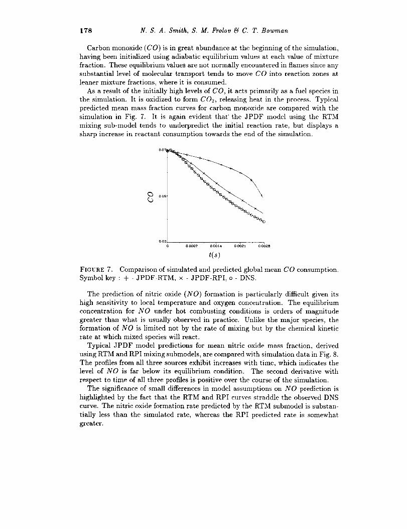
Carbon monoxide (CO) is in great abundance at the beginning of the simulation,

having been initialized using adiabatic equilibrium values at each value of mixture

fraction. These equilibrium values are not normally encountered in flames since any

substantial level of molecular transport tends to move CO into reaction zones at

leaner mixture fractions, where it is consumed.

As a result of the initially high levels of CO, it acts primarily as a fuel species in

the simulation. It is oxidized to form C02, releasing heat in the process. Typical

predicted mean mass fraction curves for carbon monoxide are compared with the

simulation in Fig. 7. It is again evident that' the JPDF model using the RTM

mixing sub-model tends to underpredict the initial reaction rate, but displays a

sharp increase in reactant consumption towards the end of the simulation.

ooz

0 05

003

oooo? ooG14 ooG2, 00028

FIGURE 7. Comparison of simulated and predicted global mean CO consumption.


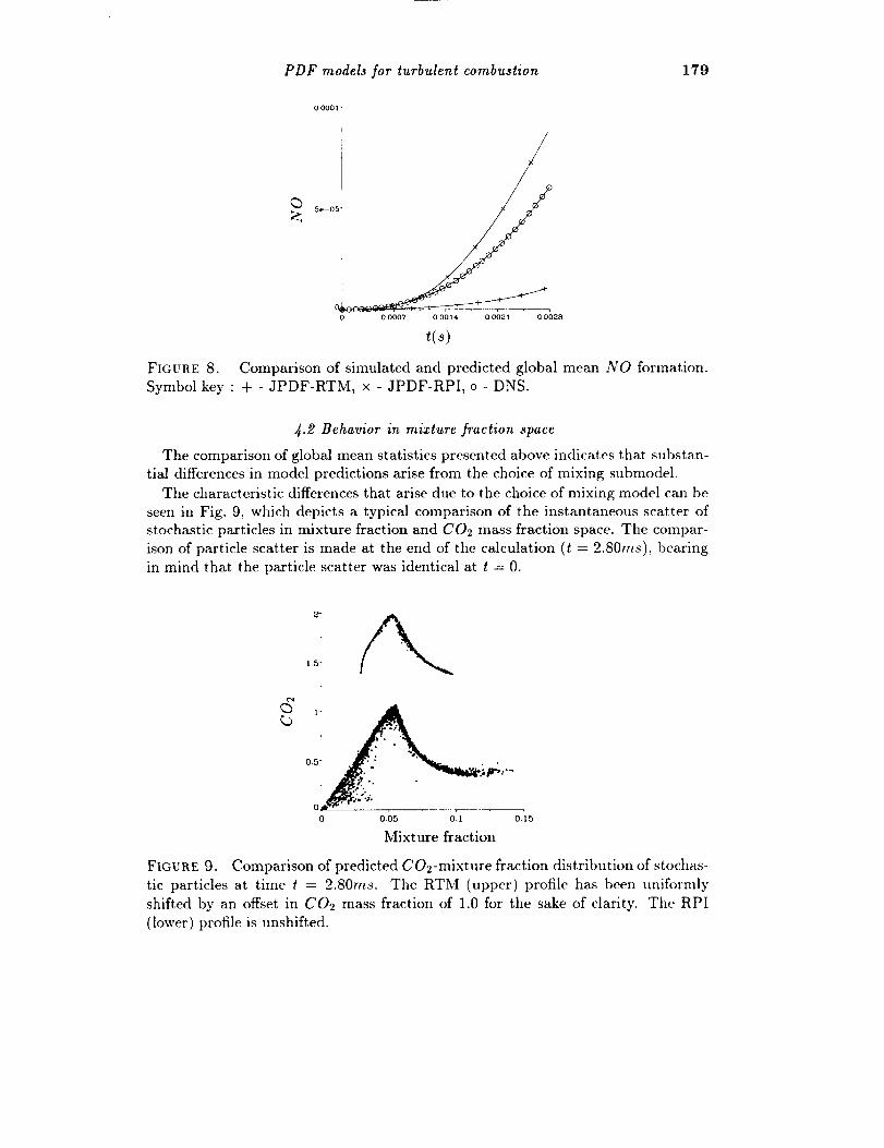
The prediction of nitric oxide (NO) formation is particularly difficult given its

high sensitivity to local temperature and oxygen concentration. The equilibrium

concentration for NO under hot combusting conditions is orders of magnitude

greater than what is usually observed in practice. Unlike the major species, the

formation of NO is limited not by the rate of mixing but by the chemical kinetic

rate at which mixed species will react.

Typical JPDF model predictions for mean nitric oxide mass fraction, derived

using RTM and RPI mixing submodels, are compared with simulation data in Fig. 8.

The profiles from all three sources exhibit increases with time, which indicates the

level of NO is far below its equilibrium condition. The second derivative with

respect to time of all three profiles is positive over the course of the simulation.

The significance of small differences in model assumptions on NO prediction is

highlighted by the fact that the RTM and RPI curves straddle the observed DNS

curve. The nitric oxide formation rate predicted by the RTM submodel is substan-

tially less than the simulated rate, whereas the RPI predicted rate is somewhat

greater.


O0001"

5e-05"

...... . , r ,

00007 0 O014 00021 0-0028

_(_)

FIGURE 8. Comparison of simulated and predicted global mean NO formation.


4.2 Behavior in mixture fraction space

The comparison of global mean statistics presented above indicates that substan-

tial differences in model predictions arise from the choice of mixing submodel.

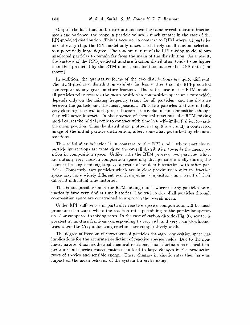
The characteristic differences that arise due to the choice of mixing model can be

seen in Fig. 9, which depicts a typical comparison of the instantaneous scatter of

stochastic particles in mixture fraction and CO: mass fraction space. The compar-

ison of particle scatter is made at the end of the calculation (t = 2.80ms), bearing

in mind that the particle scatter was identical at t = 0.

0.5

0.

0 0,05 Ol 0.15

Mixture fraction

FIGURE 9. Comparison of predicted CO2-mixture fraction distribution of stochas-

tic particles at time t = 2.80ms. The RTM (upper) profile has been uniformly

shifted by an offset in C02 mass fraction of 1.0 for the sake of clarity. The RPI

(lower) profile is unshifted.

180 N. S. A. Smith, S. M. Frolov _ C. T. Bowman

Despite the fact that both distributions have the same overall mixture fraction

mean and variance, the range in particle values is nmch greater in the case of the

RPI-modeled distribution. This is because, in contrast to YtTM where all particles

mix at every step, the RPI model only mixes a relatively small random selection

to a potentially large degree. The random nature of the RPI mixing model allows

unselected particles to remain far from the mean of the distribution. As a result,

the kurtosis of the RPI-predicted mixture fraction distribution tends to be higher

than that predicted by the RTM model, and for that matter the DNS data (not

shown).

In addition, the qualitative forms of the two distributions are quite different.

The RTM-predicted distribution exhibits far less scatter than its RPI-predicted

counterpart at any given mixture fraction. This is because in the RTM model,

all particles relax towards the mean position in composition space at a rate which

depends only on the mixing frequency (same for all particles) and the distance

between the particle and the mean position. Thus two particles that are initially

very close together will both proceed towards the global mean composition, though

they will never interact. In the absence of chemical reactions, the RTM mixing

model causes the initial profile to contract with time in a self-similar fashion towards

the mean position. Thus the distribution plotted in Fig. 9 is virtually a contracted

image of the initial particle distribution, albeit somewhat perturbed by chemicalreactions.

This self-similar behavior is in contrast to the RPI model where particle-to-

particle interactions are what drive the overall distribution towards the mean po-

sition in composition space. Unlike with the RTM process, two particles which

are initially very close in composition space may diverge substantially during the

course of a single mixing step, as a result of random interaction with other par-

ticles. Conversely, two particles which are in close proximity in mixture fraction

space may have widely different reactive species compositions as a result of theirdifferent individual time histories.

This is not possible under the RTM mixing model where nearby particles auto-

matically have very similar time histories. The trajectories of all particles through

composition space are constrained to approach the overall mean.

Under ttPI, differences in particular reactive species compositions will be most

pronounced in zones where the reaction rates pertaining to the particular species

are slow compared to mixing rates. In the case of carbon dioxide (Fig. 9), scatter is

greatest at mixture fractions corresponding to very rich and w_ry lean stoichiome-

tries where the CO_-influencing reactions are comparatively weak.

The degree of freedom of movement of particles through composition space has

implications for the accurate prediction of reactiw_ species yields. Due to the non-

linear nature of non-isothermal chemical reactions, small fluctuations in local tem-

perature and species concentrations can lead to large changes in the production

rates of species and sensible energy. These changes in kinetic rates then have an

impact on the mean behavior of the system through mixing.


10

6.67

C)

3.33

. v

0 0.04 0.08

Mixture fraction

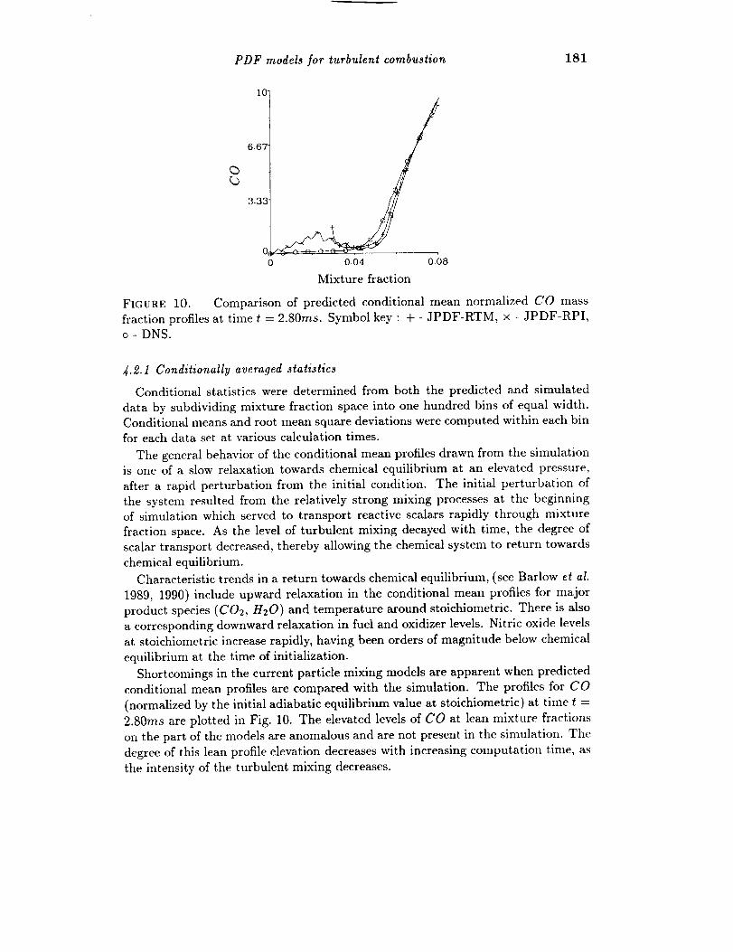
Comparison of predicted conditional mean normalized CO mass× - JPDF-RPI,

FIGURE 10.

fraction profiles at time t = 2.80ms. Symbol key : + - JPDF-RTM,

o - DNS.

4.2.1 Conditionally averaged statistics

Conditional statistics were determined from both the predicted and simulated

data by subdividing mixture fraction space into one hundred bins of equal width.

Conditional means and root mean square deviations were computed within each bin

for each data set at various calculation times.

The general behavior of the conditional mean profiles drawn from the simulationis one of a slow relaxation towards chemical equilibrium at an elevated pressure,

after a rapid perturbation from the initial condition. The initial perturbation of

the system resulted from the relatively strong mixing processes at the beginning

of simulation which served to transport reactive scalars rapidly through mixture

fraction space. As the level of turbulent mixing decayed with time, the degree of

scalar transport decreased, thereby allowing the chemical system to return towards

chemical equilibrium.

Characteristic trends in a return towards chemical equilibrium, (see Barlow et al.

1989, 1990) include upward relaxation in the conditional mean profiles for major

product species (C02, H20) and temperature around stoichiometric. There is also

a corresponding downward relaxation in fuel and oxidizer levels. Nitric oxide levels

at stoichiometric increase rapidly, having been orders of magnitude below chemical

equilibrium at the time of initialization.

Shortcomings in the current particle mixing models are apparent when predicted

conditional mean profiles are compared with the simulation. The profiles for CO

(normalized by the initial adiabatic equilibrium value at stoichiometric) at time t =

2.80ms are plotted in Fig. 10. The elevated levels of CO at lean mixture fractions

on the part of the models are anomalous and are not present in the simulation. The

degree of this lean profile elevation decreases with increasing computation time, as

the intensity of the turbulent mixing decreases.

182 N. S. A. Smith, S. M. Frolov 64 C. T. Bowman

0.6

J

0i0 0.04 0.08

Mixture fraction

FIGURE 11. Comparison of predicted conditional mean normalized temperature

profiles at time t = 2.80r_s. Symbol key : + - JPDF-RTM, x - JPDF-RPI, o -DNS.

The equations for the diffusive transport of reactive scalar mass fractions in mix-

ture fraction space (see Klimenko 1990) indicate that the negative curvature of the

conditional mean CO profile in mixture fraction space must result in a local de-

crease in the CO mass fraction profile. Similarly, chemical reactions should drive

conditional mean CO levels downward. There is no obvious physical explanation

as to how the observed elevated profiles could have been produced from the initialcondition.

A similar anomalous effect can be seen in the normalized conditional mean tem-

perature profiles in Fig. 11, where the modeled mixing processes have caused the

lean portion of the temperature profile to be depressed below the expected equi-

librium line. The temperature depression is more substantial at earlier times and

seems to be responsible for the early underprediction of mean pressure rise seen in

Fig. 5.

It is evident that the profile deviations are due to shortcomings in both the RPI

and RTM mixing models. In effect, the models allow particles to mix towards a

mean position that can be very far from their local region of composition space.

Thus, in the case of the RPI model, particles at very lean mixture fractions are

just as likely to mix with other particles at very rich mixture fractions as those

immediately adjacent to themselves. The RTM model effectively allows the same

interaction by constraining particles to mix along trajectories towards the overall

mean position.

In reality, a fluid parcel is not free to mix with any other fluid parcel; it is instead

bound to interact with those in its immediate vicinity in composition space. Parcels

in a fluid continuum cannot jump between separated locations in composition space,

given a certain time step, without having an impact upon the intervening composi-

tions. In the case of the conditional mean CO profile of Fig. 10, the elevated levels

on the lean side of the reaction zone can only exist if the CO values at stoichiometric


500-

250

O,0 0.04 0.08

Mixture fraction

FIGURE 12. Comparison of predicted conditional mean NO mass fraction [ppm]

profiles at time t = 2.80ms. Symbol key : + - JPDF-RTM, x - JPDF-RPI, o -DNS.

are more elevated still. There is no possibility of counter-gradient transport in the

simulation given the assumptions employed.

Turning to the prediction of nitric oxide (NO) formation, a comparison of condi-

tional mean profiles from the models and the simulation can be made from Fig. 12.It is clear that in all cases the formation of NO is strongly centered on the high

temperature reaction zones around stoichiometric. Of the two predictions, those of

the RPI model seem to best match the simulation profile at lean and rich mixture

fractions in capturing the transport of NO to inert zones in mixture fraction space.

An explanation for the significant discrepancy between the two model predictionsfor NO can be found in the difference between the conditional mean and variance

profiles of temperature. Throughout the calculations, the particles in the vicinity

of the reaction zone have a slightly higher conditional mean temperature under the

RPI model than the RTM model. Further, the level of conditional variance in the

temperature under the RPI model is many times greater than what is observed

under the RTM model.

The RPI model predicts a slightly higher conditional temperature variance than

the simulation, around stoichiometric, while having conditional mean temperature

values similar to the prediction. Given the high nonlinear sensitivity of NO forma-

tion to temperature, it is reasonable to speculate that this difference in conditional

variance may be the cause of the observed NO discrepancy.

5. Discussion

It is reasonable to assert that the RPI mixing model as described above seems to

perform better than the RTM mixing model under the conditions examined. The

overall prediction of mean species yields by the RPI-JPDF combination is superior

to that seen for the RTM-JPDF combination in the tests conducted.

184 N. S. A. Smith, S. M. Frolov _4 C. T. Bowman

The RPI model seems to incorporate significant conditional root mean square

deviations ill reactive species levels in mixture fraction space. This in turn may

allow better prediction the formation of thermochemicalty sensitive species such as

NO. Indeed, in cases where highly nonlinear phenomena such as extinction behavior

is to be predicted, the RTM approach would be unable to capture the significant

contributions made by particles that are far from the conditional mean profiles.

Both models, however, seem to suffer from a "long range mixing" problem. That

is to say that particles are allowed to freely mix with other particles that are far

removed in mixture fraction space, without having any effect at all oil particles that

lie in the intervening space.

The Kolmogorov _calar scale (Tlk), defined below (where rk is the Kolmogorov

time scale, and _ is the mean scalar dissipation rate), describes the characteristic

fluctuations in a conserved scalar which are present at the smallest eddy sizes, i.e.

the level of scalar fluctuations which are diminished by molecular diffusion alone.

,k -(X_rk) '/_ (9)

After making an assumption about the relationship between the scalar dissipation

rate, the scalar variance, and the turbulent time scale, it is possible to express qk

approximately as given below.

_k (X< _,2 >1/2 /Rc_/4 (10)

As the turbulent Reynolds number (Ret) in the simulation performed in this

study was rather low, the Kolmogorov scalar scale was on the order of one fifth

of the entire range of mixture fraction space. In practical turbulent reactors, one

might expect this value to be substantially lower.

Using the Kolmogorov scalar scale as a guide for the case studied here, it seems

unlikely that any particle would be able to mix on a molecular level with any other

particle that is any further than Ar/ = 0.03 distant.

It may be appropriate to attempt to modify the RPI mixing model presented here

so as to limit the range in mixture fraction space over which particles are allowed

to interact. In so doing, a greater number of particle interactions would be required

in each time step so as to correctly model the overall d('cay rate in mixture fractionvariance.

Chen and Kollmann (1994) suggest a modified RPI model which better represents

molecular diffusion by limiting the range over which particles can interact. No men-

tion of a criteria for this critical range was mentioned, but perhaps the Kolmogorov

scalar scale could be used in this capacity. To the best of the authors' knowledge,

this scheme has yet to be implemented for testing.

6. Comments

This preliminary work has served to illustrate the effective differences between

different mixing sub-models employed in a scalar JPDF model for nonprelnixedturbulent combustion.


The simulation conditions were admittedly difficult to model, given that the non-

premixed reaction zones were initially quite thin compared to both the physical and

mixture fraction scales of the domain. Nevertheless, practical multi-cellular calcu-

lations using JPDF methods will likely involve discretizations with cell Reynolds

and DamkShler numbers of the same order as that encountered in the simulation.

In that regard, the insight obtained here could be of some use in selecting a mixing

sub-model for practical usage.

It would seem that of the two mixing sub-models tested, the Random-Particle-

Interaction (RPI) model proved both to be more accurate in prediction, and also

to exhibit more of the qualitative characteristics of the mixing processes observed

in the simulation. Both mixing sub-models were found to exhibit non-physical

behavior in the sense that particles were free to interact over too wide a range in

mixture fraction space.The RPI model seems to be best suited for modification to include some limitation

on mixing interaction distances in mixture fraction space. The implementation and

testing of this modification as described in the discussion and by Chen and Kollmann

(1994) is a project for future work in this area.

Further, as computational resources become available it would be valuable to

simulate a ttlree dixnensional case of the conditions studied here. This would be done

to determine if important effects have been neglected in the current simulation and

would have the advantage of carrying a much larger number of statistical sample

points in the analysis.

REFERENCES

ANAND, M. S., & POPE, S. B. 1987 Calculations of premixed turbulent flames

by pdf methods. Combu_t. Flame. 67, 127-142.

BARLOW, R. S., DIBBLE R. W., & FOURGETTE D. C. 1989 Departure from

chemical equilibrium in a lifted hydrogen flame. Sandia Report SAND89-8627.

BAHLOW, R. S., DIBBLE, R. W., CHEN, J.-Y., & LUCHT, R. P. 1990 Effect of

DamkShler number on super-equilibrium OH concentration in turbulent non-

premixed jet flames.. Combust. Flame. 82,235.

CHEN, J.-Y. 1993 Stochastic Modeling of Partially Stirred Reactors. Presented at

the Fall Meeting of the Western States Section of the Combustion Institute.

Menlo Park, California.

CHEN, J.-Y. 1996 Private communication.

CHEN, J.-Y., CHANG, W.-C., & KOSZYKOWSKI, M. L. 1995 Numerical Simula-

tion and Scaling of NOx Emissions from Turbulent Hydrogen Jet Flames with

Various Amounts of Helium Dilution. Combust. Sci. Tech. 110, 505.

CIJEh', J.-Y. & KOLLMANN, W. 1988 PDF Modeling of Chemical Nonequilib-

rium Effects in Turbulent Nonpremixed Hydrocarbon Flames. Proceeding_ of

the Twenty-Second Symposium (International) on Combustion. The Combus-

tion Institute. 645-653.

186 N. S. A. Smith, S. M. Frolov gfl C. T. Bowman

CIIEN, J.-Y. & KOLLMANN, W. 1992 PDF Modeling and Analysis of Thermal

NO Formation in Turbulent Nonpremixed Hydrogen-Air Jet Flames. Combust.

Flame. 88, 397-412.

CHEN, J.-Y. & KOLLMANN, W. 1994 Comparison of prediction and measurement

in nonpremixed turbulent flames, in Turbulent Reacting Flows, F. A. Williams

& P. A. Libby (eds), Academic Press Ltd. 211-308

CORREA, S. M. 1993 Turbulence-Chemistry Interactions in the Intermediate Regime

of Premixed Combustion. Combust. Flame. 93, 41-60.

COaaEa, S. M., & POPE, S. B. 1992 Comparison of a Monte Carlo PDF/Finite

Volume Mean Flow Model with Bluff-Body Raman Data. Proceedings of the

Twenty-Fourth Symposium (International) on Combustion. The CombustionInstitute. 279-285.

DOPAZO, C. 1975 Probability function approach for a turbulent axisymmetric

heated jet: centerline evolution. Phys. Fluids. 18, 397.

DOPAZO, C. 1979 On conditioned averages for intermittent turbulent flows. J.

Fluid Mech. 81,433.

FrtOLOV, S. M. 1996 Private communication.

JANICKA, J., KOLBE W., _ KOLLMANN W. 1979 Closure of the transport equa-

tion for the probability density of function of scalar fields. J. Nonequilib. Ther-

modyn. 4, 27.

JAN1CKA, J., & KOLLMANN, W. 1978 A Two-Variables Formalism for the Treat-

ment of Chemical Reactions in Turbulent He-Air Diffusion Flames. ProceedingL,

of the Seventeenth Symposium (International) on Combustion. The Combustion

Institute. 421-430.

KLIMENKO, A. Yu. 1990 Multicomponent diffusion of various admixtures in tur-

bulent flow. Fluid Dynamics. 25, 327-334.

POPE, S. B. 1981 A Monte Carlo Method for the PDF Equations of Turbulent

Reactive Flow. Combust. Sci. Tech. 25, 159-174.

POPE, S. B. 1982 An improved turbulent mixing model. Comb. Sci. Tech. 28, 131.

POPE, S. B. 1985 PDF Methods for Turbulent Flows. Prog. Energy Sci. Comb.

11, 119-192.

POPE, S. B. 1990 Computations of Turbulent Combustion: Progress and Chal-

lenges. Proceedings of the Twenty-Third Symposium (International) on Com-bustion. The Combustion Institute. 591-612.

SMITH, N. $. A., BILGErt, R. W., CANTER, C. D., BARLOW, R. $., & CHEN,

J.-Y. 1993 A Comparison of CMC and PDF Modelling Predictions with

Experimental Nitric Oxide LIF/Raman Measurements in a Turbulent H2 Jet

Flame. Combust. Sci. Tech. 105, 357-375.

SMITH, N. S. A., BILGErt, R. W., CARTEr(, C. D., BAaLOW, R. S., & CHEN J.-

Y. 1996 Radiation Effects on Nitric Oxide Formation in Turbulent Hydrogen

Jet Flames Diluted with Helium. Submitted to Combustion and Flame.

Evaluation of joint probability density function models ... · Evaluation of joint probability...

Documents

Transcript of Evaluation of joint probability density function models ... · Evaluation of joint probability...