Evaluation of Geometric Accuracy and Image Quality

of an On-Board Imager (OBI)

Master of Science Thesis in Medical Radiation Physics

Milos Djordjevic

Supervisor: Bruno Sorcini, PhD

Stockholm University and Karolinska Institute

2

ABSTRACT In this project several tests were performed to evaluate the performance of an On-Board Imager® (OBI) mounted on a clinical linear accelerator. The measurements were divided into three parts; geometric accuracy, image registration and couch shift accuracy, and image quality. A cube phantom containing a radiation opaque marker was used to study the agreement with treatment isocenter for both kV-images and cone-beam CT (CBCT) images. The long term stability was investigated by acquiring frontal and lateral kV images twice a week over a 3-month period. Stability in vertical and longitudinal robotic arm motion as well as the stability of the center-of-rotation was evaluated. Further, the agreement of kV-image and CBCT center with MV image center was examined. A marker seed phantom was used to evaluate and compare the three applications in image registration; 2D/2D, 2D/3D and 3D/3D. Image registration using kV-kV image sets were compared with MV-MV and MV-kV image sets. Further, the accuracy in 2D/2D matches with images acquired at non-orthogonal gantry angles was evaluated. The image quality in CBCT images was evaluated using a Catphan® phantom. Hounsfield unit (HU) uniformity and linearity was compared with planning CT. HU accuracy is crucial for dose verification using CBCT data. The geometric measurements showed good long term stability and accurate position reproducibility after robotic arm motions. A systematic error of about 1 mm in lateral direction of the kV-image center was detected. A small difference between kV and CBCT center was observed and related to a lateral kV detector offset. The vector disagreement between kV- and MV-image centers was > 2 mm at some gantry angles. Image registration with the different match applications worked sufficiently. 2D/3D match was seen to correct more accurately than 2D/2D match for large translational and rotational shifts. CBCT images acquired with full-fan mode showed good HU uniformity but half-fan images were less uniform. In the soft tissue region the HU agreement with planning CT was reasonable while a larger disagreement was observed at higher densities. This work shows that the OBI is robust and stable in its performance. With regular QC and calibrations the geometric precision of the OBI can be maintained within 1 mm of treatment isocenter. Key-words: Image-guided radiotherapy, Cone-beam CT, OBI, Quality Assurance.

3

CONTENTS List of abbreviations 5 1 INTRODUCTION 6 2 MATERIAL AND METHODS 9

2.1 THE ON-BOARD IMAGER SYSTEM 9 2.1.1 Cone Beam CT 11 2.1.2 Image registration 12

2.2 GEOMETRIC ACCURACY OF THE OBI 15 2.2.1 Isocentric setup verification of the OBI 16

2.2.1.a Frontal and lateral kV images set ................................................................................. 17 2.2.1.b Accuracy and stability during gantry rotation.............................................................. 18 2.2.1.c MV and kV image center agreement............................................................................ 18 2.2.1.d Linearity of vertical kV-detector arm motion .............................................................. 19

2.2.2 Magnification accuracy in kV images 19 2.2.3 CBCT reconstruction center 19

2.3 IMAGE REGISTRATION AND COUCH SHIFT ACCURACY 20 2.3.1 Translational phantom displacements 21 2.3.2 Combined rotational and translational shifts 22

2.4 IMAGE QUALITY 23 2.4.1 kV image QA 23 2.4.2 CBCT image QA 23

2.4.2.a HU uniformity and stability.......................................................................................... 25 2.4.2.b HU Linearity ................................................................................................................ 26 2.4.2.c In-slice Geometry ......................................................................................................... 27 2.4.2.d Image slice width ......................................................................................................... 27 2.4.2.e Spatial resolution and image contrast........................................................................... 28 3 RESULTS AND DISCUSSION 29

3.1 GEOMETRIC ACCURACY OF THE OBI 29 3.1.1 Isocentric setup verification of the OBI 29

3.1.1.a Frontal and lateral kV images set ................................................................................. 29 3.1.1.b Accuracy and stability during gantry rotation.............................................................. 31 3.1.1.c MV and kV image center agreement............................................................................ 36 3.1.1.d Linearity of vertical detector arm motion .................................................................... 37

3.1.2 Magnification accuracy in kV images 38 3.1.3 CBCT reconstruction center 39

3.2 IMAGE REGISTRATION AND COUCH SHIFT ACCURACY 41 3.2.1 2D/2D match application 41

3.2.1.a AP and RL kV images.................................................................................................. 41 3.2.1.b MV-MV and MV-kV images....................................................................................... 44 3.2.1.c 2D/2D match with kV images acquired at oblique angles ........................................... 44

3.2.2 Marker Match application 45 3.2.3 3D/3D match application 48 3.2.4 Physical couch shift 48

3.3 IMAGE QA 49 3.3.1 kV image quality 49 3.3.2 CBCT image QA 50

3.3.2.a HU uniformity and stability.......................................................................................... 51 3.3.2.b HU Linearity ................................................................................................................ 53 3.3.2.c In-slice Geometry ......................................................................................................... 55

4

3.3.2.d Image Slice Width........................................................................................................ 56 3.3.2.e Spatial Resolution......................................................................................................... 56 3.3.2.f Low contrast resolution................................................................................................. 57 4 CONCLUSIONS 60 ACKNOWLEDGEMENTS 62 REFERENCES 63 APPENDIX 65

5

List of abbreviations

AP Anterior-Posterior

ART Adaptive Radiation Therapy

BB Ball Bearing

CBCT Cone-beam Computed Tomography

COR Center of Rotation

CT Computed Tomography

DRR Digitally Reconstructed Radiograph

FF Full-Fan

FOV Field of View

HF Half-Fan

HU Hounsfield Unit

IGRT Image Guided Radiation Therapy

kV Kilo-voltage

kVD Kilo-voltage Detector

kVS Kilo-voltage Source

Lat Lateral

Lng Longitudinal

MV Megavoltage

MVD Megavoltage Detector

OBI On-Board Imager

PTV Planning Target Volume

CTV Clinical Target Volume

QA Quality Assurance

QC Quality Control

RL Right-Left lateral

ROI Region of Interest

SAD Source-Axis Distance

SID Source-Imager Distance

SNR Signal to Noise Ratio

SSD Source Surface Distance

Vrt Vertical

6

1 INTRODUCTION The objective of radiation therapy is to accomplish tumor control while sparing the normal

tissue from radiation induced complications. Modern techniques, such as 3D conformal and

intensity modulated radiotherapy (3D-CRT, IMRT), manage to shape radiation doses to

closely conform the tumor volume, reducing the dose to critical structures. These techniques

may allow dose escalation to the target increasing the probability of tumor control (Zelefsky

et al 2002). Clinical use of more precise radiotherapy machines and more accurate dose

planning algorithms require, however, an exact knowledge of the target position, not only at

the planning stage but also at the actual treatment times. Conventionally, the tumor position is

determined at one single time during treatment planning using computed tomography (CT)

images. This information may not be accurate during treatment delivery due to patient setup

errors and organ motion (Balter et al 1995). The treatment is usually delivered in 20 to 40

fractions, allowing for inter-fractional motions. The result is an inherent geometric

uncertainty, limiting the probability of achieving an accurate radiation treatment (Hector et al

2000, Webb et al 2006). To compensate for this uncertainty additional margins are added to

the clinical target volume (CTV) to form the planning target volume (PTV) (ICRU report 50

1993, ICRU report 62 1999). These margins result in increased normal tissue irradiation. By

localizing the target position before each treatment fraction, it may be possible to reduce the

margins. In IMRT the radiation is delivered with steep dose gradients allowing smaller

margins to be used if target position is verified on-line. Significant dose escalations may be

possible if geometric uncertainties can be reduced from current levels of 5-10 mm to 3 mm

(Jaffray and Siewerdsen 2000). In regions with significant organ motion this is only possible

if the target is localized before each treatment session (Martinez et al 2001). The vital need of

accurate target positioning has resulted in vast advances and increased research in the field of

image guided radiation therapy (IGRT) (Mackie et al 2003, Mohan et al 2005, McBain et al

2006, Sorcini and Tilikidis 2006, Sorcini 2006). Conventionally the patient setup has been

verified using megavoltage (MV) radiographs acquired with the linear accelerator. With a

kilo-voltage (kV) x-ray source mounted on-board a linear accelerator, e.g. an On-Board

Imager (OBI), an increase in bony structure contrast enables more reliable setup corrections

(Schewe et al 1998, Jaffray et al 1999). Still, 2-dimensional (2D) radiographic projections do

not provide adequate soft-tissue contrast to localize the tumor itself. The new techniques of

7

acquiring cone-beam CT (CBCT) images by rotating an x-ray system with the gantry allow

soft tissue visibility (Jaffray et al 2000, Jaffray et al 2002, Oldham et al 2005, Li et al 2006a).

In April 2004 an On-Board Imager® system (Varian Medical Systems, Inc., Palo Alto, CA,

USA) was installed on one of the linear accelerators at the Karolinska University Hospital,

Stockholm, Sweden. The OBI system is used to correct for patient setup errors and inter- and

intra-fractional organ motion. Both radiographic projections and volumetric CBCT images

can be acquired with the OBI. CBCT data may be used for patient dose verification and inter-

fractional treatment re-planning, correcting for organ movement and deformation (Lo et al.

2005, Xing et al 2006, Yang et al 2007). Adjusting the treatment plan to anatomical changes

during the treatment course is referred to as adaptive radiotherapy (ART).

In this thesis, the performance of the OBI is evaluated in terms of its geometric accuracy,

algorithm accuracy and image quality. The main focus is on the parameters determining the

accuracy when correcting the target position. This includes the mechanical precision of the

OBI and the accuracy in mechanical couch correction, as well as the implementation of the

match applications provided by the OBI system. Further, the CBCT image quality and

Hounsfield unit (HU) accuracy is evaluated. HU accuracy is crucial if CBCT data shall be

used in ART (Yang et al 2007). Several of the tests performed in this paper are aimed to be

used in a quality assurance (QA) program. The new technology introduced by the OBI

requires a comprehensive QA program to maintain the requirements of the system established

at the time of commissioning. Quality control (QC) tests should be reasonable, simple and fast

to perform, yet reliable to confirm consistency in the performance of the OBI. QC tests for the

OBI should include: safety and functionality, geometric accuracy, and image quality.

Additional dose measurements of the CBCT should be performed when used clinically at

every treatment session. Safety and functionality tests should be performed daily and may be

combined with the x-ray tube warm-up in the mornings. Appropriate tests are described in the

maintenance manual [Maintenance Manual On-Board Imager (OBI) (Varian medical systems,

Inc., Palo Alto, CA , 2006)] and are not discussed further in this thesis. QC tests concerning

the geometric accuracy are the most critical part as the OBI is used to correct patient position

and these should be performed frequently until confidence in the stability is achieved. A

simple phantom containing one radio opaque marker, a cube phantom, was used to estimate

both the accuracy and stability of the OBI. Initially, image quality tests have to be frequent.

8

Once consistency in imaging performance has been verified, the tests may be performed less

frequently.

The measurements in this thesis are divided in three parts; geometric accuracy of the OBI,

image registration, and image quality. The two first parts evaluate both mechanical

parameters as well as some software functionalities, e.g. the accuracy of the different match

applications and the CBCT reconstruction center. The image quality is evaluated for the

radiographic and the CBCT modes.

9

2 MATERIAL AND METHODS 2.1 THE ON-BOARD IMAGER SYSTEM

The OBI is an imaging device mounted on the linear accelerator used to verify treatment

position on-line or off-line. The OBI consists of two robotic arms, called ExactArms, one

holding an x-ray source, i.e. kilo-voltage source (kVS), and the other one holding an

amorphous silicon (a-Si) flat panel detector, i.e. kilo-voltage detector (kVD). The ExactArms

are mounted perpendicular to the gantry of the linear accelerator, figure 1. The OBI system is

rotated with the gantry. Linear motion of the ExactArms is allowed in longitudinal and

vertical directions. In addition the kVD can be moved laterally. The direction of motion of the

OBI ExactArms should be distinguished from the directions defining the couch position.

Position values for the ExactArms are relative the MV beam path; vertical motion means

towards or away from the MV beam axis and lateral motion of the kVD is motion parallel to

the MV beam, see figure 1(b) and (c).

The Exactarm is constructed in similar way as the human arm; a hand holding the kVS or

kVD, a forearm and an upper arm, connected with a wrist, an elbow joint and a shoulder joint.

The position of the ExactArms can be changed with the hand pendants in the treatment room

or remotely in the operator room with the OBI control console. The ExactArms are equipped

with collision detectors and interlock systems. The kVS consists of x-ray tube and collimator.

The possible tube voltages are 40 kV to 150 kV. The travel ranges of the collimator blades are

50 mm to 250 mm. The target angle, i.e. anode angle, is 14° and two possible focal spot

values, 0.4 mm and 0.8 mm, are possible.

The kVD unit consists of a flat panel imager with an anti-scatter grid (PaxScan 4030CB,

Varian Medical Systems, Inc., Palo Alto, CA). The active imaging area is approximately 40 ×

30 cm2 and consists of a 2048 × 1536 matrix of a-Si thin-film transistors and photodiodes in

combination with a luminescent phosphor, i.e. scintillating material. In most applications the

so-called half resolution mode (2 × 2 binning) is used resulting in 1024 × 768 logical pixels.

The phosphor layer consists of Tl doped CsI and acts as an intensifying screen by absorbing

incident x-rays and emitting visible light that is detected by the photodiodes in the a-Si panel.

This type of digital detector is often referred to as an indirect detection flat panel system

10

(Bushberg 2002). The detector is enclosed in a plastic cover to protect the detector in case of

collision. The possible source-to-imager distances (SID) are 100.0 cm to 182.5 cm.

(a) (b)

(c)

Figure 1. (a) Varian clinical linear accelerator with an On-Board Imager® (OBI) consisting of two robotic arms; one holding an x-ray source (kVS) and one holding a flat panel imager (kVD). The mega voltage detector (MVD) is also extracted. (b) The coordinate system for couch/patient position: Lat = +Right/-Left, Vrt = +Ant/-Post and Lng = +Inf/-Sup. (c) Lateral and vertical motion of the kVD are relative the MV beam axis.

The OBI provides three different imaging modes; 2-D radiographic acquisition, fluoroscopic

image acquisition and 3-D cone-beam computed tomography (CBCT). There are two modes

for 2D digital radiography; single standard and single high quality. 2D radiographs acquired

with the OBI are called kilo voltage, kV, images to distinguish from mega voltage, MV,

images acquired with the accelerator. kV images and CBCT images are used to correct for

setup errors and inter-fractional organ motion. CBCT data may also be used to recalculate the

patient dose at the corrected position and even be used for inter-fractional treatment re-

planning, i.e. ART. The fluoroscopic imaging mode is used for pre-treatment setup

verification of the respiratory gating system (RPMTM, Varian Medical Systems, Inc., Palo

Alto, CA), i.e. to validate gating thresholds. The gating system is used to account for intra-

fractional respiratory motion.

11

2.1.1 Cone Beam CT

A conventional third generation CT (Bushberg 2002), uses a fan beam and image projections

are acquired on single rows of detector elements during a scan. The beam is rotated once for

each slice. Modern multi-slice CT uses several rows, up to 64 rows, of detector elements in

each rotation. A cone-beam CT uses a cone shaped beam and acquires projections onto a 2D

detector. All slices within the selected scan width are reconstructed from one single gantry

rotation. When the OBI is used as a cone beam CT 675 projections are acquired over one

gantry rotation. The 2D projected images are reconstructed into a 3D volumetric data set

using a filtered back-projection technique. During the scan every 10th projection is displayed

on the monitor. The CBCT allows two different acquisition geometries, full-fan (FF) or

half-fan (HF) depending on the size of the treatment site, figure 2. With FF mode a maximum

field-of-view (FOV) of 24 cm is possible at SID = 150 cm. This geometry is mainly used on

skull and head and neck patients. HF mode is used for body scans and allows a maximum

reconstructed FOV of about 45 cm at SID = 150 cm. When a FOV larger than 24 cm is

selected, the CBCT acquisition is automatically switched to HF mode. When HF geometry is

used, the kVD is shifted 15 cm laterally with the blades in the kVS cutting off approximately

half of the beam aligning the beam axis at one edge of the detector. During the scan each part

of the image is seen only once, except a small volume at the center of the FOV. Bowtie filters

are used to compensate for the smaller thickness at the edges of the target volume compared

with the central part. Different bowtie filters are used for the two geometries. The two

scanning modes are calibrated separately. The maximum longitudinal scan width is 15.5 cm

and 13.7 cm for FF and HF geometry respectively. Slice thicknesses between 1.0 mm and 5.0

mm in 0.5 mm increments can be reconstructed. Three options for the resolution of the

reconstructed volume are available; 128 × 128 pixels, 256 × 256 pixels and 512 × 512 pixels.

The scan time equals the time for one gantry rotation, approximately one minute. The

additional time for reconstruction depends on the reconstruction parameters (slice-width, scan

range, FOV, number of pixels etc.) and can be up to 3 minutes. To acquire a CBCT image the

ExactArms are extracted and rotated 185° to start position followed by the scan. After the

scan the gantry is rotated back to 0° and the arms are retracted. The total time for acquisition,

reconstruction, registration (3D/3D image match) and correction of couch position will add up

to 10 minutes to the treatment time. Scans can be acquired in both directions; clock-wise and

counter clock-wise.

12

Figure 2. The two geometries for a CBCT scan; (a) full-fan and (b) half-fan. The kVD is shifted when using half fan. Different bowtie filters are used with the two geometries.

2.1.2 Image registration

The treatment plan is based on images acquired with a conventional CT. If the target volume

shall receive the planned dose the target has to be positioned according to the plan at the time

of treatment. Images acquired with the OBI just prior to treatment are used to verify the target

position. Tumor motion and errors in patient setup can be corrected for by matching the

acquired images with reference images. The image registration can be performed either

according to anatomical structures or using seed implants, i.e. radio opaque markers. The

different match applications allow both automatic and manual matches. Once the images

coincide, the amount of couch adjustment in lateral, vertical, longitudinal directions as well as

couch rotation needed are displayed as couch shift values, see figure 3. The couch shift values

are rounded off to nearest integer millimeter. When the shift values are downloaded to the

accelerator the couch is moved remotely to adjust the patient position. There are three

different match applications available; 2D/2D match, MarkerMatch (2D/3D) and 3D/3D

match.

13

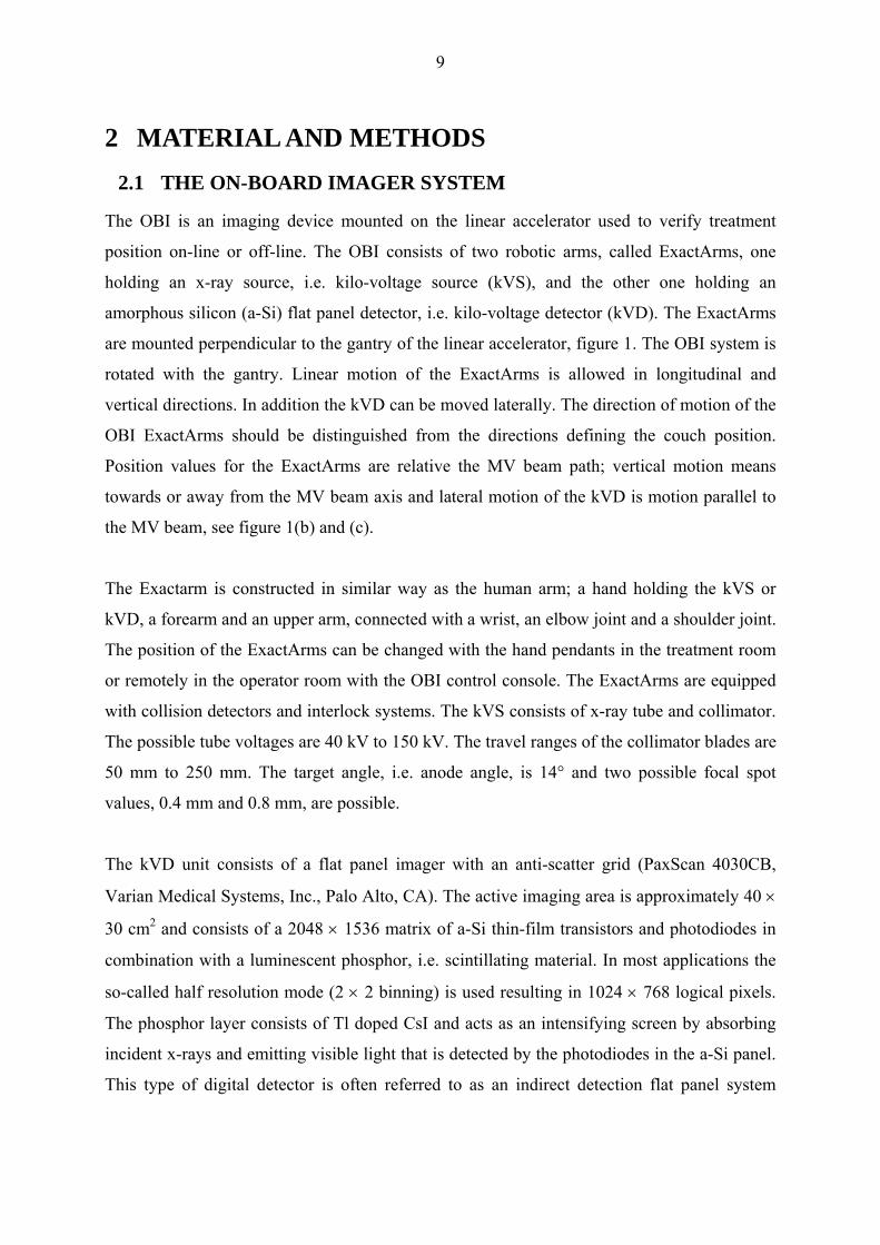
Figure 3. A CBCT image (in blue) is matched with the reference CT (in orange). The upper-right view shows only the reference CT. The amounts of couch corrections needed in the different directions are displayed below the images.

The 2D/2D match application uses two images acquired in the treatment room and two

reference images, digital reconstructed radiographs (DRRs) or simulator radiographs. DRRs

are created from the planning CT images. To match the two set of images independently, they

should be perpendicular to each other. Usually anterior-posterior (AP) images and right-left

(RL) images are used. The AP image set gives the deviation in lateral and longitudinal couch

position and the RL image set gives the deviation in vertical and longitudinal couch position.

Images may be acquired with the OBI system only, i.e. kV images, to perform a kV-kV

match, or with the Linear accelerator, i.e. MV images, to perform a MV-MV match or one

image with each modality to perform a MV-kV match. When performing a MV-kV 2D/2D

match an AP MV-image and a RL kV-image are generally used. At image registration the

acquired images are superimposed onto the reference images. A green digital graticule can be

displayed showing the treatment planning origin in the reference image. A red digital

graticule can be displayed showing the center of the acquired image. The two graticules will

14

initially coincide. The reference images are moved to match corresponding structures in the

acquired images. When the match is complete the distance between the two graticules will

correspond to the displacement of the images. The amount of couch shift needed will be

displayed on the monitor. The application includes automatic match algorithms for several

anatomical structures. The automatic matching process is based on mutual information

techniques. However, if 2D/2D match is used to match marker implants manual match must

be used, to avoid matching bone structures in anatomy.

The Marker Match application makes use of fiducial markers to detect and correct target

movements. Implanted gold markers are used as surrogate for the tumor due to limited soft

tissue visibility in kV images. At least three radio opaque markers have to be implanted in the

target to make use of the Marker Match algorithm. When using the Marker Match application

the reference images have to be CT data sets. The CT reference images are used to localize

the markers relative treatment planning isocenter (reference origin). By acquiring an

orthogonal image set with the OBI the markers can be localized at each treatment session.

When performing the match, the coordinates of the markers in the kV images are compared

with the coordinates of the markers in the reference CT. The markers are first detected in the

reference CT and then digital cross-marks are displayed in the two kV images at the

corresponding coordinates. The digital cross-marks are then matched individually with the

marker seeds in the acquired images. As when performing a 2D/2D match the acquired

images may be kV images or MV images or one of each. As radiographic 2D-projections are

matched with a 3D CT set Marker Match is also referred to as 2D/3D match. When using the

automatic match application it is important to choose region of interest carefully to include all

markers both in the reference image and in the acquired radiographs. The detection of the

markers in the reference CT will not be saved for subsequent session and therefore the

procedure has to be repeated each treatment session. The time to perform image registration

with the automatic Marker Match application is about 1 min.

With the 3D/3D match application a CBCT scan acquired with the OBI is matched with the

planning CT. The CBCT images are superimposed onto the planning CT images in three

different views; transversal, sagittal and coronal views. A fourth window will display only the

reference CT set. The images can be displayed in grayscale or in colors. When displaying in

colors the CBCT images will be blue and the reference images red. When performing the

match the CBCT images are moved to match with the structures in the reference images. The

15

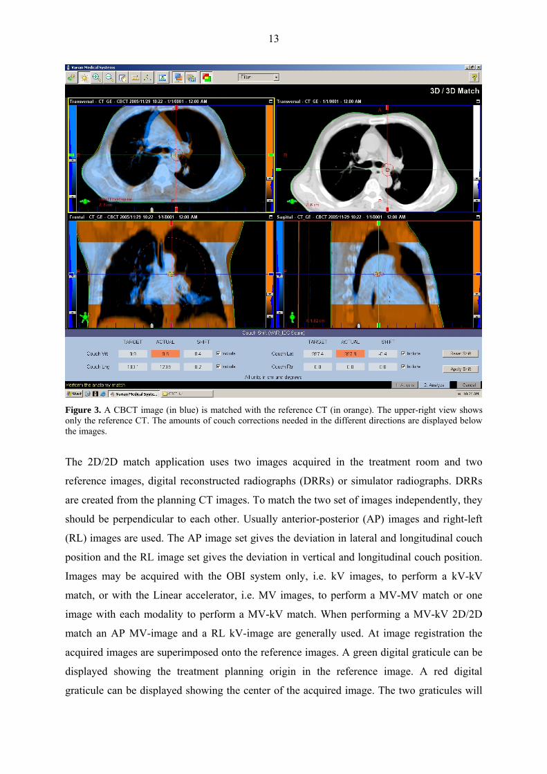
images are matched in all three views. Both manual and automatic match options are

available. Figure 4 illustrates the three different match applications used in image registration.

Figure 4. Schematic figure of the three different match applications available with the OBI system.

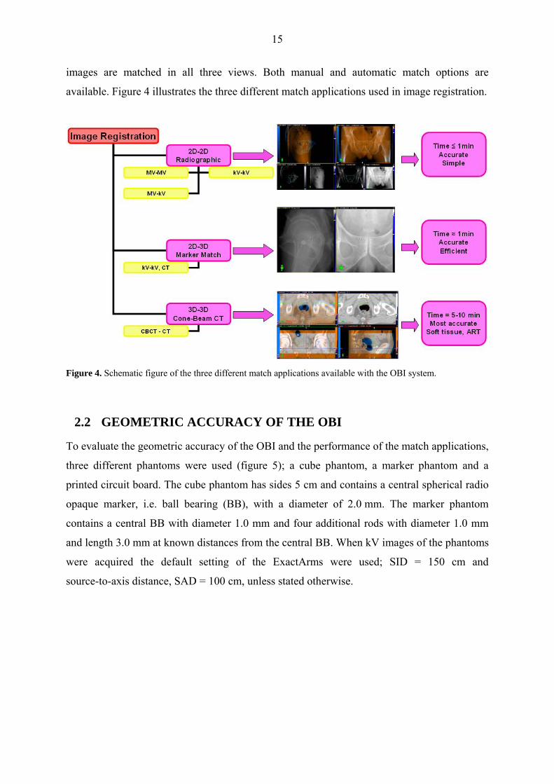
2.2 GEOMETRIC ACCURACY OF THE OBI

To evaluate the geometric accuracy of the OBI and the performance of the match applications,

three different phantoms were used (figure 5); a cube phantom, a marker phantom and a

printed circuit board. The cube phantom has sides 5 cm and contains a central spherical radio

opaque marker, i.e. ball bearing (BB), with a diameter of 2.0 mm. The marker phantom

contains a central BB with diameter 1.0 mm and four additional rods with diameter 1.0 mm

and length 3.0 mm at known distances from the central BB. When kV images of the phantoms

were acquired the default setting of the ExactArms were used; SID = 150 cm and

source-to-axis distance, SAD = 100 cm, unless stated otherwise.

16

Figure 5. Three phantoms used to verify the geometric accuracy of the OBI; (a) a cube phantom, (b) a marker phantom and (c) a printed circuit board phantom.

2.2.1 Isocentric setup verification of the OBI

In radiation therapy treatment with an OBI one has to distinguish between at least the

isocenter of the planning CT, the linear accelerator, the lasers and the OBI. When using the

CBCT mode, the reconstructed CBCT image center should further agree with treatment

isocenter. For the linear accelerator, one has to distinguish between gantry isocenter and the

actual treatment beam isocenter. If the gantry rotation is circular symmetric the gantry

isocenter will coincide with the axis-of-rotation, i.e. SAD is constant with gantry angle. In

general, SAD will vary slightly with gantry angle. Further, the agreement of the treatment

beam isocenter with the gantry isocenter will depend on the beam collimation. Thus, the

treatment isocenter might not be a well defined point. However, the intersections of the beam

axis at different gantry angles should be confined within an acceptable volume (Podgorsak

2003). With an OBI the treatment beam isocenter, the gantry isocenter, the calibrated

treatment isocenter (lasers), the OBI isocenter as well as the reconstructed CBCT isocenter

should all be confined within a sphere with an acceptable diameter. Figure 6 shows an

illustration of different isocenters involved in radiation therapy treatment.

The OBI system is used for on-line corrections of the patient position to accurately target the

tumor. A digital graticule generated by the OBI application can be displayed showing the kV

image center which is assumed to coincide with the treatment isocenter. When a 2D/2D match

is performed, the center of the graticule is superimposed onto the reference origin (treatment

planning isocenter). Then, a successful match will result in correct treatment position

according to the plan only if the kV image center agrees with the treatment isocenter. This

requires that the OBI is isocentric, i.e. that the kV beam axis and the kVD imaging center

coincides with treatment isocenter. The isocenter agreement can be tested by positioning a

17

radio opaque marker in the calibrated treatment isocenter, i.e. the intersections of the wall

lasers, and acquire kV images. In the image the marker should coincide with the center of the

digital graticule. This test relies on accurately calibrated wall lasers. In all tests performed in

this thesis the position of any phantom used has also been verified using the field light

crosshair of the accelerator. The field light crosshair has been assumed to agree with the

treatment beam axis. Further, it is assumed that the wall lasers and the field light crosshair are

independently checked and accurately represent the treatment isocenter. The geometric QA

tests evaluate the accuracy in the isocentric setup of the OBI and the stability of the

ExactArms over time. Most of these tests can be performed with the cube phantom or the

marker phantom, or any phantom containing a radio opaque marker.

Figure 6. A schematic illustration of different possible isocenter motion trajectories involved in radiotherapy

treatment with an OBI. The calibrated isocenter is the intersection of the wall lasers.

2.2.1.a Frontal and lateral kV images set

This test was performed to evaluate the agreement between the digital graticule displayed in

the OBI application and the calibrated treatment isocenter for AP and RL images, that are

most commonly used when performing 2D/2D match. The center of the cube phantom was

positioned in the treatment isocenter using wall lasers and the field light crosshair and AP and

RL images were acquired. In the OBI console the BB was zoomed in and the digital graticule

was displayed. The vector displacement of the BB from the center of the digital graticule was

measured as well as its x- and y-components, see figure 7. These measurements were repeated

18

twice a week during September through December, 2006. Once a week additional

measurements were performed with kV images acquired in Posterior-Anterior (PA) and Left-

Right (LR) directions.

Figure 7. The x-component of the vector displacement is the projected transverse displacement and the y-component is the axial displacement, i.e. longitudinal direction.

2.2.1.b Accuracy and stability during gantry rotation

In this assessment the accuracy and stability of the ExactArms during gantry rotation were

examined. The agreement between the kV image center and the treatment isocenter, at any

gantry angle, will depend on; (1) the agreement of the kV beam isocenter with the treatment

isocenter and (2) the kVD position relative the kV beam axis. kV images of the cube phantom

were acquired in 15° intervals over one gantry rotation. This was repeated once a week for

nine weeks with two imager positions; SID = 150 cm and SID = 140 cm.

2.2.1.c MV and kV image center agreement

In this test the kV image center is compared with the MV image center. The advantage of this

test is that the difference in image position will be independent of phantom position. If the

MV detector (MVD) is accurately calibrated this can be seen as a direct comparison of the kV

image center and the actual treatment beam isocenter. However, due to the uncertainty in

accuracy of the MVD position, this should be seen merely as a test of agreement between the

two imaging systems. By acquiring both kV and MV images over a full gantry rotation any

instability of the ExactArms may be distinguished from gantry instabilities. The alignment of

the cube phantom was first checked with a kV image set and then with a MV image set by

measuring the displacement of the BB from the digital graticules in both image sets. The

19

difference in the displacement was recorded. This was repeated once a week for ten weeks.

Additional measurements were done with PA images and LR images. Three measurements

were done over full gantry rotation acquiring kV and MV images at 30° intervals.

2.2.1.d Linearity of vertical kV-detector arm motion

This test was done to see whether a change of vertical detector position, i.e. change in SID,

has any lateral or longitudinal components. The printed circuit board phantom, figure 5 (c),

was placed on the treatment couch and centered at the isocenter with the field light crosshair.

AP images were acquired with source-to-surface distance, SSD = 100 cm and SID varying

between 130 cm and 170 cm in 10 cm intervals. The image displacements at the different

kVD positions were compared. By moving the kVD back and forth between the different

positions we could also see if the same position was reproduced after a vertical kVD motion.

2.2.2 Magnification accuracy in kV images

To evaluate the magnification accuracy in kV images the printed circuit board was used with

the same setup and vertical kVD positions as in section 2.2.1.d. At each SID, with

SSD = 100 cm, the lengths of the sides of the 10 cm × 10 cm square in the printed circuit

board, as well as the diagonals, were measured. The measured distances were recorded and

compared with the expected distances. This was repeated with the couch moved ± 10 cm in

vertical direction, i.e with SSD = 110 cm and SSD = 90 cm. The measured distances were

compared with the expected distances corrected for beam divergence.

2.2.3 CBCT reconstruction center

To study the CBCT reconstruction isocenter (CBCT center) the cube phantom was positioned

with the BB in the calibrated treatment isocenter. CBCT scans were acquired with both FF

and HF mode using a slice width of 1.0 mm. In the analyze environment of the 3D/3D match

application the CBCT images are superimposed on the reference CT images. Reference CT

images of the cube phantom had been prepared in the treatment planning system (Eclipse,

Varian medical systems, Inc., Palo Alto, CA) with the BB centered at the planning treatment

isocenter (see section 2.3). The following investigations were performed to study the

20

agreement between CBCT center and (a) the calibrated treatment isocenter, (b) the kV image

center, and (c) the MV image center.

(a) To estimate the CBCT center accuracy, the vector distance between the BB and the

planning isocenter (center of reference image) as well as the lateral and vertical components

were measured in the transversal view. The lateral and vertical components of the

displacement were also measured in the coronal and sagittal views, respectively. The

longitudinal displacement component was measured in the frontal and sagittal views.

(b) Orthogonal kV images were acquired to compare the CBCT center used in 3D/3D

matches with the kV image center used in 2D/2D matches. The alignment of the BB in the kV

images was compared with the alignment in the CBCT images. At five occasions kV

projections were acquired at 30° intervals over one gantry rotation to compare the CBCT

reconstruction center with the center of rotation of the OBI, i.e. mean kV isocenter.

(c) Orthogonal MV images were also acquired to compare the CBCT center with the MV

image center.

2.3 IMAGE REGISTRATION AND COUCH SHIFT ACCURACY

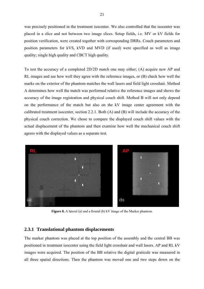
The marker phantom (figure 5b) was used to examine the accuracy of the three different

match applications. Figure 8 shows an AP and a RL kV radiograph of the marker phantom.

The marker phantom is held by an assembly with three steps. From the top position on the

assembly it can be shifted 2.0 cm and 3.5 cm in the superior (S), posterior (P) and right (R)

directions.

CT images of the marker phantom were acquired with the planning CT. The transversal CT

slices were then used to construct a 3D volume planning image in Eclipse. The center marker

in the 3D volume reference image was relocated to the treatment isocenter. This was done by

adjusting the user origin to the center of the center marker in the 3D image. When treatment

fields are created the isocenter of the fields will be in the position of the initial user origin and

the coordinates of the isocenter will be relative the new users origin. We repositioned the

treatment isocenter to the new user origin by setting the coordinates of the isocenter to x = 0

cm, y = 0 cm and z = 0 cm. In this way, the center marker in the 3D image of the phantom

21

was precisely positioned in the treatment isocenter. We also controlled that the isocenter was

placed in a slice and not between two image slices. Setup fields, i.e. MV or kV fields for

position verification, were created together with corresponding DRRs. Couch parameters and

position parameters for kVS, kVD and MVD (if used) were specified as well as image

quality; single high quality and CBCT high quality.

To test the accuracy of a completed 2D/2D match one may either; (A) acquire new AP and

RL images and see how well they agree with the reference images, or (B) check how well the

marks on the exterior of the phantom matches the wall lasers and field light crosshair. Method

A determines how well the match was performed relative the reference images and shows the

accuracy of the image registration and physical couch shift. Method B will not only depend

on the performance of the match but also on the kV image center agreement with the

calibrated treatment isocenter, section 2.2.1. Both (A) and (B) will include the accuracy of the

physical couch correction. We chose to compare the displayed couch shift values with the

actual displacement of the phantom and then examine how well the mechanical couch shift

agrees with the displayed values as a separate test.

RL AP

(a) (b)

Figure 8. A lateral (a) and a frontal (b) kV image of the Marker phantom.

2.3.1 Translational phantom displacements

The marker phantom was placed at the top position of the assembly and the central BB was

positioned in treatment isocenter using the field light crosshair and wall lasers. AP and RL kV

images were acquired. The position of the BB relative the digital graticule was measured in

all three spatial directions. Then the phantom was moved one and two steps down on the

22

assembly, i.e. 2.0 cm and 3.5 cm in the S, P, and R directions. This was repeated with the

marker phantom shifted in opposite directions by starting at the lowest and mid positions on

the assembly, i.e. 2.0 cm and 3,5 cm in the left (L), anterior (A) and inferior (I) directions.

The assembly was also rotated 180° and the phantom shifted in the L, P and I directions. At

the new position new AP and RL images were acquired. The displacement of the BB was

measured in the second image set. The differences in the displacements in the two image sets

were recorded and compared with the expected shifts. A 2D/2D match was performed and the

couch shift values generated by the OBI application were compared with the actual shift of

the phantom. The couch shift values were further compared with the distances measured with

the measuring tool in the second image set. The shift was then reset and a Marker Match was

performed (this was not done with all phantom shifts). The couch shift values of the Marker

Match were compared with those of the 2D/2D match and the expected couch shift. 2D/2D

matches were also performed with MV images (MV-MV match) and with one MV image and

one kV image (MV-kV match). Further, 2D/2D matches with kV images acquired at other

gantry angles than AP and RL projections were performed. To compare the different match

applications CBCT images were also acquired and 3D/3D matches performed.

The shift reproducibility was evaluated by measuring the physical shift of the couch and

comparing with the displayed values. The agreement was recorded separately. The change in

position of the couch was measured using measuring devises with 0.05 mm accuracy.

2.3.2 Combined rotational and translational shifts

The marker phantom was positioned with the center marker in the calibrated treatment

isocenter. The couch was manually rotated ±1°, ±2°, ±4°, ±6° and ±10°. At the new position

the phantom was adjusted so that the field light crosshair matched the cross-marks on the top

side of the phantom. Then the couch was rotated back to the initial position. Thus the

phantom was rotated the desired amount relative the field light crosshair and the couch. AP

and RL kV-images were acquired followed by a 2D/2D match and a Marker Match. Then a

CBCT scan was acquired followed by a 3D/3D match. The couch shift values for the three

match types were recorded. Matches with combined rotational and translational shifts were

also performed. The phantom was rotated ±2° and ±5° and translated ±1.0 cm in lateral,

vertical and longitudinal directions.

23

2.4 IMAGE QUALITY

Image QA measurements were performed to evaluate the quality of kV images and CBCT

images, to find suitable tests for regular QA and to establish required limits in imaging

performance. The main issue in image QA is to verify consistency in image quality.

2.4.1 kV image QA

To investigate the spatial resolution and contrast resolution in kV images different Leeds

phantoms (Leeds test objects Ltd, North Yorkshire, UK, www.leedstestobjects.com) were

used. To monitor the spatial resolution a HUTTNER type 18 phantom was used. This is a

rectangular, 55 mm × 45 mm, 0.1 mm thick lead brick with 21 groups of bar patterns ranging

from 0.5 line pairs per mm (lp/mm) to 5 lp/mm. A NOISE TO.N3 low contrast sensivity

phantom was used to monitor the contrast resolution. The phantom is a circular plate, 180

mm in diameter, containing 19 details with 11 mm diameters with nominal contrast ranging

from 16 % to 0.7 %. An additional phantom, TO.10., was used for overall contrast detail

detect ability. This phantom contains 108 details, 12 different sizes ranging from 11 mm to

0.25 mm in diameter with 9 different contrasts.

The single high quality mode was used for radiographic image quality tests. The OBI

application offers approximately 20 preset x-ray techniques for different anatomical sites,

patient sizes and beam directions (AP or RL). The preset techniques can be manually

adjusted. Most preset techniques uses 70 kVp to 80 kVp while the mAs value varies more

extensively. The largest patient group that the OBI is used on is prostate patients. Therefore

we used the option; pelvis, AP, medium size for spatial resolution and pelvis, AP, small size

for contrast resolution. These options use the following x-ray techniques; 75 kVp, 80 mA and

40 ms respectively 30 ms. 1.0 mm copper was used as scattering material and placed in front

of the kVS. The phantoms were placed on the kVD and AP images were acquired with

SID = 150 cm.

2.4.2 CBCT image QA

CBCT imaging is a trade-off between image quality, patient dose and scanning time. CBCT is

aimed to be used for two main purposes; treatment position verification and treatment dose

verification/reconstruction. Image contrast, resolution and geometry are important parameters

24

for accurate image registration. To perform dose calculations with the CBCT requires

agreement between Hounsfield unit (HU) and relative electron density (Dong et al 2006, Lo et

al 2005, Yang et al 2007). Therefore HU stability, uniformity and linearity were investigated

and compared with planning CT.

A Catphan® 504 phantom (The Phantom Laboratory Inc., Greenwich, NY,

www.phantomlab.com) was used to evaluate overall CBCT image quality (figure 9). The

Catphan phantom is cylindrical with an outer diameter of 20 cm and an inner diameter of

15 cm. The phantom is divided in several sections or modules; each module containing

different test objects. The box supplied with the phantom was positioned on the couch and the

phantom was suspended over one edge. With help of the lasers the phantom was leveled. The

phantom needed to be scanned only once for a given CBCT protocol to perform the different

tests in the modules. Measurements were done with both FF mode and HF mode, using

different slice thicknesses raging from the smallest possible, 1.0 mm, to 5.0 mm. 1.0 mm and

2.5 mm slices were used as standard protocols to check performance stability of the CBCT.

The X-ray tube current was 80 mA and the generator energy was 125 kV, which is the

standard setting. We used the largest number of pixels possible for the reconstruction matrix,

512×512 pixels. The scan ranges used were 15.5 cm for FF mode and 13.7 cm for HF mode,

which are the maximum widths for each mode. The standard FOVs used was 24 cm for the FF

mode, and 25 cm for HF mode, which are the maximum and minimum FOV for respective

mode. These FOVs were selected to minimize the influence of pixel size when comparing the

two modes. The larger pixel size with increasing FOV will decrease the spatial resolution and

increase the low contrast resolution, i.e. increase signal-to-noise ration (SNR) in each voxel.

With these FOVs the pixel size was approximately 0.5 mm with both modes. Measurements

with HF mode were also performed with maximum reconstruction FOV, 45 cm, which is

clinically more relevant for body scans. Additional measurements were performed with other

scan ranges, pixel numbers and FOVs.

The different investigations performed with the Catphan phantom were; HU stability and

uniformity, HU linearity, in-slice geometry, slice thickness, spatial resolution and low contrast

resolution. Additional tests for the HF mode were done with an RMI® phantom

(Gammex-RMI Ltd, Nottingham, UK, www.gammex.com), consisting of a Solid Water®

cylinder with a diameter of 33 cm, approximating the size of an average pelvis.

25

Figure 9. The Catphan® 504 phantom containing several modules used in CT image QA is shown to the left. A

schematic of the phantom is shown to the right [Catphan® 504 manual insert, (Greenwich, NY, The Phantom

Laboratory)].

2.4.2.a HU uniformity and stability

The HU, i.e. CT number, is a value assigned to a pixel corresponding to the radiodensity

relative water in the corresponding voxel. The HU is defined as, (Bushberg 2002):

SFyx

yxHUw

w ×−

=μ

μμ ),(),( (1)

where ),( yxμ is the mean attenuation value in the voxel corresponding to pixel (x,y) and wμ

is an estimated attenuation value of water at the effective energy of the beam used. SF = 1000

is a scale factor.

The CTP 486 module in the Catphan phantom contains a uniform material that is designed to

have HU values within 2 % (20 HU) of water’s density at standard scanning protocols

[Catphan®500 and 600 Manual (Greenwich, NY, The Phantom Laboratory, Inc. 2004,

www.phantomlab.com)]. The area profile tool in the CBCT application was used to measure

the mean HU in a region of interest (ROI). One ROI was selected at the center of the image

slice and four ROIs were located at peripheral positions symmetrically around the center, see

figure 10a. The sizes of the ROIs were 10 × 10 mm2, covering approximately 400 pixels. The

26

mean value and standard deviation in each ROI was recorded. The spatial uniformity (SU) can

be defined as the HU difference between the maximum and minimum measured mean HU

value, or as a percentage difference in apparent linear attenuation coefficient relative the

attenuation in water:

100(min)(max)×

−=

SFHUHUSU (2)

The variation in HU values between the ROIs should be within ±20 HU, [CBCT on OBI:

Customer Acceptance Procedure, CAP (2.2.3), (Varian medical systems, Inc., Palo Alto, CA,

2005)]. In-slice line profiles were also measured in horizontal, vertical and diagonal

directions. Further, the mean of the five mean HU values in the ROIs was calculated to

evaluate the HU stability over several measurements. The mean HU value in each ROI was

also measured in neighbouring slices to check for any inter-slice variation.

The standard deviation (σ) of the pixel values in each ROI was used to estimate the quantum

noise, i.e. stochastic fluctuation of HU value within the ROI. The relative noise can be

expressed as fluctuations in apparent linear attenuation coefficient relative that of water:

100×=SF

Noise σ (3)

2.4.2.b HU Linearity

The radiodensity at standard temperature and pressure (STP) is defined as zero HU for

distilled water and as -1000 HU for air. The relationship between electron density and HU for

biological tissue has been expressed as two linear regions; air to water and water to bone

(Parker et al 1979) (Sage et al 1998). The Catphan phantom is recommended by Varian to be

used when calibrating HU linearity for the CBCT. The CTP 404 module contains seven

different cylindrical high contrast targets with known electron densities, see figure 10b. The

diameter of the targets is 12 mm. The area profile tool was used to measure the mean HU

value in each target. A ROI size of 5×5 mm2 was used which covers about 100 pixels and is

small enough to not be close to the interface between target and background. In conventional

CT images ROIs covering > 25 pixels are usually considered enough to avoid influence of

27

statistical fluctuations between pixels. The measured values were compared with the expected

[Catphan®500 and 600 Manual (Greenwich, NY, The Phantom Laboratory, Inc. 2004.)]. The

HU values should be within ± 40 HU of the expected values [CBCT on OBI: Customer

Acceptance Procedure, CAP (2.2.3)].

2.4.2.c In-slice Geometry

The CTP 404 module contains four 3 mm diameter holes, one with a Teflon pin, which are

positioned 50 mm apart (figure 10b). The distances between the centers of the holes were

measured to verify the magnification accuracy and circular symmetry in the CBCT images.

The circular symmetry of the image may also be tested by comparing the lengths of the

diameter of the inner cylinder of the phantom when measured along the vertical (y-) axis and

when measured along the horizontal (x-) axis. The diameter should be 150 mm. Any

measurement should fall within an accuracy of 1 % of the actual distance [CBCT on OBI:

Customer Acceptance Procedure, CAP (2.2.3)].

2.4.2.d Image slice width

The CTP404 module contains two pair of wire ramps inclined 23° relative the axial plane.

The projection of the wires in the transversal images will be parallel to the x-respective y-axis

(figure 10b). The image slice width, Z, can thus be estimated as the length of the wire as

measured in the transversal image multiplied by tan(23°). The estimated length of the wire in

the transversal image is the FWHM of the CT number (HU) peak of the wire, [Catphan®500

and 600 Manual (Greenwich, NY, The Phantom Laboratory, Inc. 2004.)]. Thus:

Z = FWHM × tan(23°) (4)

An alternative way to estimate the slice thickness is to measure the increment between the

center of two adjacent slices. This can be estimated from the difference in position of the wire

in the transversal view in two adjacent slices multiplied by tan(23°). The slice increment can

also be directly measured in the sagittal or coronal views by zooming in the voxels. This

length should preferably agree with the estimated image slice width using equation 4.

28

(a) (b)

Figure 10. Transversal CBCT slices of (a) the CTP486 and (b) the CTP404 modules. Five ROIs in the CTP486 module are used to verify HU uniformity. The CTP404 module is used to verify in-slice geometry, slice thickness and HU linearity.

2.4.2.e Spatial resolution and image contrast

The CTP528 module containing a high contrast resolution gauge ranging from 1 through 21

line pair per cm (lp/cm) was used for visual evaluation of the spatial resolution. A bar pattern

may be considered resolved if the bars can be perceived with some discernible spacing or

lowering in density between them. In case of ambiguity the line profile tool was used. To

examine the low contrast resolution the CTP515 module was used. This module contains

three groups of supra-slice targets that are 40 mm in length with diameters ranging from

2.0 mm to 15.0 mm in 1 mm steps. The three groups have nominal target contrast levels of

0.3 %, 0.5 % and 1.0 %. There are three groups of sub-slice targets with lengths 3 mm, 5 mm

and 7 mm, respectively, all with nominal target contrast of 1.0 %. The diameter of the sub-

slice targets ranges from 3.0 mm to 9.0 mm in 2 mm steps. When evaluating low contrast

resolution the window width and level has to be carefully set, a narrow window width should

be used for optimal image contrast. The spatial resolution should be greater than 6 lp/cm and

at least the 7 mm 1 % supra-slice disc (#4) in the low contrast module should be visible

[CBCT on OBI: Customer Acceptance Procedure (CAP) (2.2.3)].

29

3 RESULTS AND DISCUSSION

3.1 GEOMETRIC ACCURACY OF THE OBI

3.1.1 Isocentric setup verification of the OBI

3.1.1.a Frontal and lateral kV images set

The displacement of the BB relative the digital graticule in AP and RL kV images are shown

in figure 11 for a total of 34 measurements during a 3-month period. No geometric

calibrations of the system were performed during this period. The longitudinal displacements

in the figure are those measured in the AP images. The mean displacement and one standard

deviation (σ) for the different directions are shown in table 1. A systematic error in lateral

position of the kV image center relative the calibrated treatment isocenter of almost 1 mm was

seen in the AP images. The measurements showed stability of the OBI over the four month

period. The lateral and vertical displacement depends both on lateral ExactArm position. The

smaller variation from measurement to measurement in longitudinal position may be

explained by a better stability of the ExactArms in longitudinal direction than in lateral

direction. However, it may also be explained by the accuracy in positioning the phantom in

the different directions. The treatment couch was slightly tilted in right-left direction making

it more difficult to match the lasers with the marks on both sides of the phantom for vertical

position. When performed as a QC test we suggest an action level of ± 1.5 mm in any

direction, as the shift values in the match applications are rounded off to nearest integer

millimeter. Alternatively, only the vector displacement in the two images may be measured in

frequent QC tests. Then we suggest an action level of 2 mm. Initially, tests of kV image

center accuracy in AP and RL images should be performed frequently, e.g. weekly.

Table 1: Mean displacement of the BB in the cube phantom in 34 measurements over the period September to December, 2006.

Mean displacement ±1σ [mm]

AP radiographs RL radiographs

Lat Lng Vrt Lng

0.9 ± 0.3 -0.4 ± 0.2 0.2 ± 0.4 -0.2 ± 0.2

30

Figure 11. Long term stability of the OBI. The marker position relative the digital graticule in AP and RL images were measured twice a week over a three month period; Vrt: +Ant/-Post, Lng: +Inf/-Sup, Lat: +R/-L. The longitudinal displacement in the figure is that measured in the AP images.

To examine the reproducibility of the source and detector position when retracting and

extracting the ExactArms as well as after gantry rotation, the displacement of the BB was

measured in a series of 12 RL and AP images, acquired with the phantom in the same position

(figure 12). The OBI was rotated 90° between each acquisition and the ExactArms were

retracted and extracted after each set of acquisitions. The error bars are the estimated

uncertainty in each measurement; ± 0.15 mm (half a pixel size). The OBI system was seen to

be stable in reproducing position after gantry rotation and longitudinal motion of the

ExactArms (1σ < 0.02 mm in all directions, variation < 0.3 mm from measurement to

measurement).

In the work of Yoo et al (2006), a collaborated study of four institutions, a QA test for OBI

isocenter accuracy has been performed suggesting using only one image projection, AP or

RL. We find it incorrect to draw any conclusions about the accuracy of the OBI from images

acquired at only one gantry angle. Only if there is a complete agreement between the kV

beam isocenter and the treatment isocenter one gantry angle is enough to determine the

accuracy in kVD position. In general the OBI isocenter accuracy is determined by the

accuracy in calibration of both the kVS and the kVD. At certain gantry angles, the vector sum

31

of a kV beam isocenter offset and a kVD offset may add up to zero giving a false reliability

on the precision of the OBI. AP and RL images are most commonly used when verifying

patient position with the 2D/2D match application. It is therefore important to regularly check

the image center agreement at these gantry angles. These tests should not be seen as tests of

isocenter agreement, but tests of the accuracy and reproducibility at these specific gantry

angles.

Figure 12. A series of twelve AP and RL projections of the cube phantom to test the accuracy in repositioning of the OBI after gantry rotation and longitudinal motion of the ExactArms. The ExactArms were retracted and extracted after each set of images. The longitudinal position is that measured in the AP images. The error bars

show the estimated uncertainty in each measurement.

3.1.1.b Accuracy and stability during gantry rotation

Examples of four images acquired at gantry angles 0°, 90°, 180° and 270° are shown in

figure 13. The mean vector displacement of the BB and its x- and y-components in kV images

acquired at gantry angles 90°, 180°, 270° and 0° are shown in table 2. The y-component is the

axial displacement and corresponds always to the longitudinal displacement. The

x-component is the projected transverse displacement and corresponds to lateral displacement

for AP and PA images and to vertical displacement for RL and LR images. Figure 14 shows:

(a, b) the vector displacements R, (c) the x-component and (d) the y-component at the

different gantry angles for the 3-month period. The sum of the x-position in AP and PA

images, and in RL and LR images (e) and the difference between the y-position in AP and PA

32

images, and in RL and LR images (f) are also plotted. Figure 14(e) and (f) demonstrate the

center of rotation (COR) stability from measurement to measurement independent of phantom

position.

Figure 13. Right-left lateral (RL), anterior-posterior (AP), left-right lateral (LR) and posterior-anterior (PA) kV-images of the center BB in the cube phantom. Table 2: Mean vector displacement (R) of the BB from the digital graticule and its x- and y-components at different gantry angles, n = 12. Mean displacement ± 1σ [mm]

Projection Gantry angle kVS angle R x y

AP 90° 0° 1.0 ± 0.3 -0.9 ± 0.4 0.4 ± 0.2

LR 180° 90° 1.2 ± 0.3 -1.2 ± 0.3 0.1 ± 0.2

PA 270° 180° 0.3 ± 0.3 -0.1 ± 0.4 -0.1 ± 0.2

RL 0° 270° 0.3 ± 0.3 0.1 ± 0.3 0.2 ± 0.3

The axial position was seen accurate for lateral (both RL and LR) images and least accurate

for AP images. The variation in accuracy in axial position with gantry orientation was stable

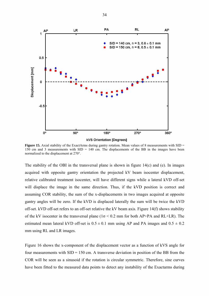
from measurement to measurement (figure 14(d) and (f)). Figure 15 shows the relative mean

axial displacement as a function of kVS angle with SID = 150 cm, n = 8, and with

SID = 140 cm, n = 3. The values have been normalized to the displacements at 270°. The

mean variation in position during gantry rotation was 0.5 ± 0.1 mm with SID = 150 cm and

0.6 ± 0.1 mm with SID = 140 cm.

33

(a) (b)

(c) (d)

(e) (f)

Figure 14. Measured displacement of the BB at four orthogonal gantry angles over a 3-month period. (a) Schematic image showing the directions in an image, (b) the vector displacements, (c) the x-components and (d) the y-components. (e) The sum of x-displacements in images acquired at opposite gantry angles to evaluate center-of-rotation stability and kVD offset. (f) Difference in y-displacements in images acquired at opposite gantry angles show long term stability but a small variation in axial position during gantry rotation.

34

Figure 15. Axial stability of the ExactArms during gantry rotation. Mean values of 8 measurements with SID = 150 cm and 3 measurements with SID = 140 cm. The displacements of the BB in the images have been normalized to the displacement at 270°.

The stability of the OBI in the transversal plane is shown in figure 14(c) and (e). In images

acquired with opposite gantry orientation the projected kV beam isocenter displacement,

relative calibrated treatment isocenter, will have different signs while a lateral kVD off-set

will displace the image in the same direction. Thus, if the kVD position is correct and

assuming COR stability, the sum of the x-displacements in two images acquired at opposite

gantry angles will be zero. If the kVD is displaced laterally the sum will be twice the kVD

off-set. kVD off-set refers to an off-set relative the kV beam axis. Figure 14(f) shows stability

of the kV isocenter in the transversal plane (1σ < 0.2 mm for both AP+PA and RL+LR). The

estimated mean lateral kVD off-set is 0.5 ± 0.1 mm using AP and PA images and 0.5 ± 0.2

mm using RL and LR images.

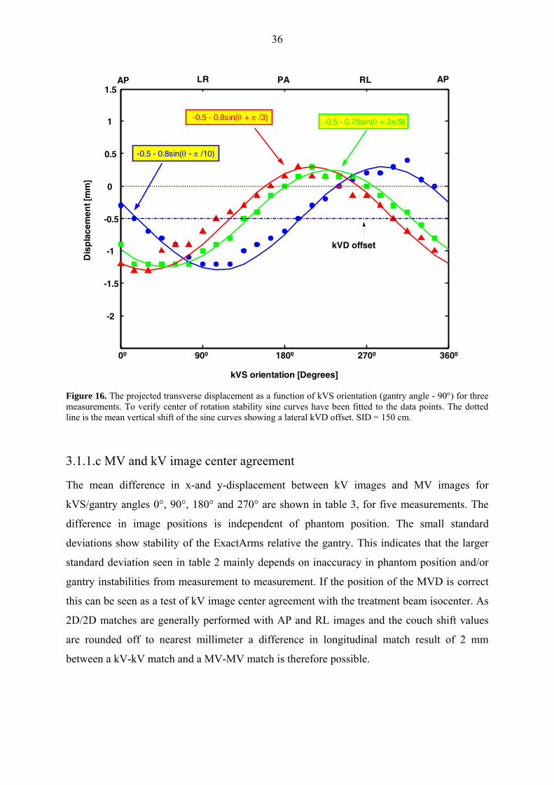
Figure 16 shows the x-component of the displacement vector as a function of kVS angle for

four measurements with SID = 150 cm. A transverse deviation in position of the BB from the

COR will be seen as a sinusoid if the rotation is circular symmetric. Therefore, sine curves

have been fitted to the measured data points to detect any instability of the Exactarms during

35

gantry rotation. In a few measurements the initial x-position was not regained after gantry

rotation, i.e. corkscrew motion. However the deviation from the initial position after

completed rotation in any measurement was ≤ 0.3 mm. Nine measurements were done with

SID = 150 cm and three with SID = 140 cm. No regular instabilities at specific gantry angles

were observed but minor variations in the smoothness of the curves were seen from

measurement to measurement. In all measurements a vertical shift of the sine curve was

observed indicating a lateral misalignment of the kVD relative the kV beam. As both the kVS

and the kVD rotates with the gantry a lateral error in kVD position should be seen as a

constant offset, i.e. a vertical shift of the sine curves. The offset was stable from measurement

to measurement with a mean of 0.5 ± 0.1 mm, in agreement with above. As the COR was seen

stable and the vertical shift of the curves independent of phantom position, the lateral kVD

off-set can be estimated from only one measurement over a gantry rotation.

The amplitude of the fitted sine curve estimates the transverse vector displacement of the BB

from the COR in the axial plane. At the angle where the sine curve has its maximum

respective minimum the kV beam is perpendicular to the transverse displacement vector

component. The mean amplitude of the fitted sine curves was 0.8 ± 0.2 mm estimating the

transverse vector displacement of the kV beam isocenter from the calibrated treatment

isocenter. The displacement of the kV beam isocenter can however not be estimated from

only one measurement due to the uncertainty in phantom position. To estimate the kV beam

isocenter displacement the kVD off-set can be subtracted from the mean of a series of

measurements in AP and RL images, as in table 1. We see that in our measurements the kVD

off-set reduces the kV image center disagreement in RL images but increases the

disagreement in AP images.

We suggest that tests to verify the isocentric setup of the OBI with gantry angles 90°, 180°,

270° and 0° are performed monthly or semi-monthly. Both the x-and y-components should be

measured to separate between the axial and transverse stability during gantry rotation. We

suggest an action level of ± 2 mm for any gantry angle.

36

0º 90º 180º 270º 360º

-2

-1.5

-1

-0.5

0

0.5

1

1.5

kVS orientation [Degrees]

Dis

pla

cem

ent [

mm

]

-0.5 - 0.8sin(θ - π /10)

AP LR PA RL AP

-0.5 - 0.8sin(θ + π /3) -0.5 - 0.75sin(θ + 2π/9)

kVD offset

Figure 16. The projected transverse displacement as a function of kVS orientation (gantry angle - 90°) for three measurements. To verify center of rotation stability sine curves have been fitted to the data points. The dotted line is the mean vertical shift of the sine curves showing a lateral kVD offset. SID = 150 cm.

3.1.1.c MV and kV image center agreement

The mean difference in x-and y-displacement between kV images and MV images for

kVS/gantry angles 0°, 90°, 180° and 270° are shown in table 3, for five measurements. The

difference in image positions is independent of phantom position. The small standard

deviations show stability of the ExactArms relative the gantry. This indicates that the larger

standard deviation seen in table 2 mainly depends on inaccuracy in phantom position and/or

gantry instabilities from measurement to measurement. If the position of the MVD is correct

this can be seen as a test of kV image center agreement with the treatment beam isocenter. As

2D/2D matches are generally performed with AP and RL images and the couch shift values

are rounded off to nearest millimeter a difference in longitudinal match result of 2 mm

between a kV-kV match and a MV-MV match is therefore possible.

37

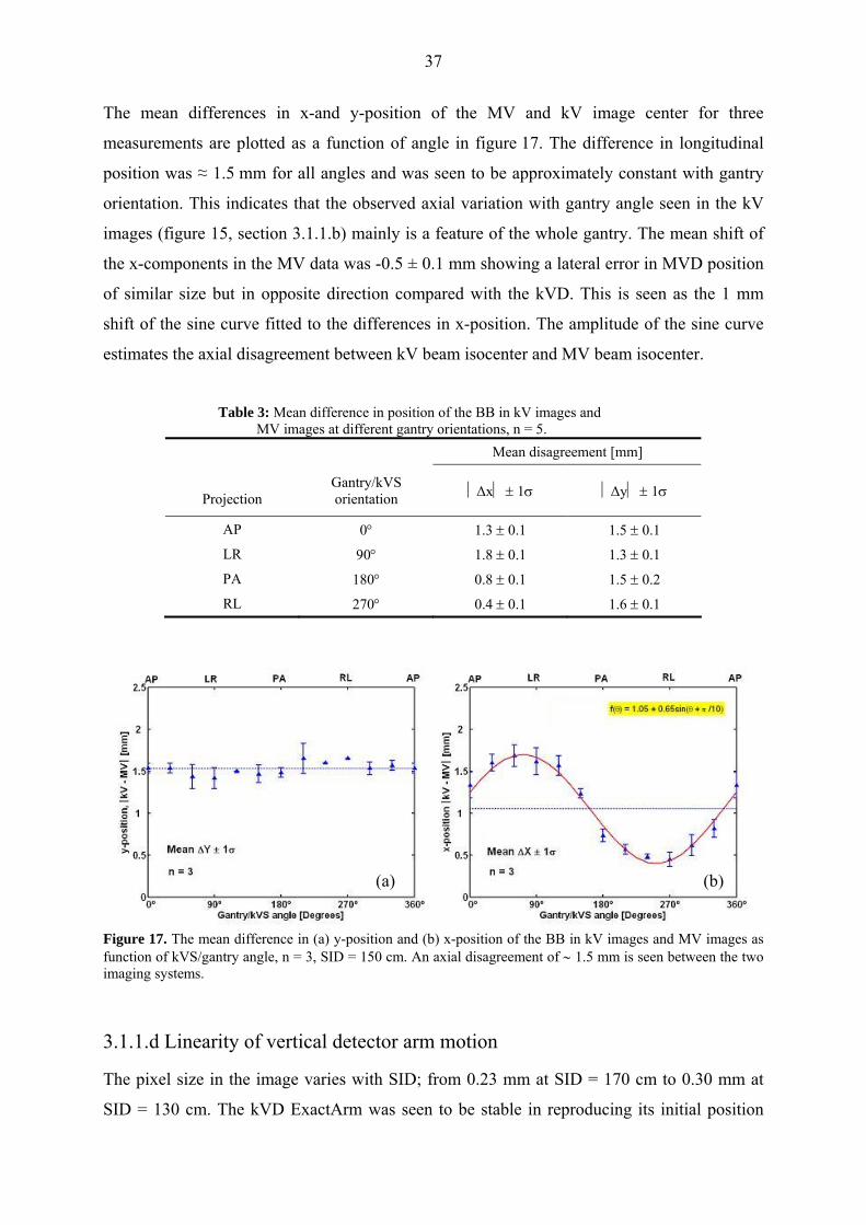
The mean differences in x-and y-position of the MV and kV image center for three

measurements are plotted as a function of angle in figure 17. The difference in longitudinal

position was ≈ 1.5 mm for all angles and was seen to be approximately constant with gantry

orientation. This indicates that the observed axial variation with gantry angle seen in the kV

images (figure 15, section 3.1.1.b) mainly is a feature of the whole gantry. The mean shift of

the x-components in the MV data was -0.5 ± 0.1 mm showing a lateral error in MVD position

of similar size but in opposite direction compared with the kVD. This is seen as the 1 mm

shift of the sine curve fitted to the differences in x-position. The amplitude of the sine curve

estimates the axial disagreement between kV beam isocenter and MV beam isocenter.

Table 3: Mean difference in position of the BB in kV images and MV images at different gantry orientations, n = 5.

Mean disagreement [mm]

Projection

Gantry/kVS orientation ⏐Δx⏐ ± 1σ

⏐Δy⏐ ± 1σ

AP 0° 1.3 ± 0.1 1.5 ± 0.1

LR 90° 1.8 ± 0.1 1.3 ± 0.1

PA 180° 0.8 ± 0.1 1.5 ± 0.2

RL 270° 0.4 ± 0.1 1.6 ± 0.1

(a) (b)

Figure 17. The mean difference in (a) y-position and (b) x-position of the BB in kV images and MV images as function of kVS/gantry angle, n = 3, SID = 150 cm. An axial disagreement of ∼ 1.5 mm is seen between the two imaging systems.

3.1.1.d Linearity of vertical detector arm motion

The pixel size in the image varies with SID; from 0.23 mm at SID = 170 cm to 0.30 mm at

SID = 130 cm. The kVD ExactArm was seen to be stable in reproducing its initial position

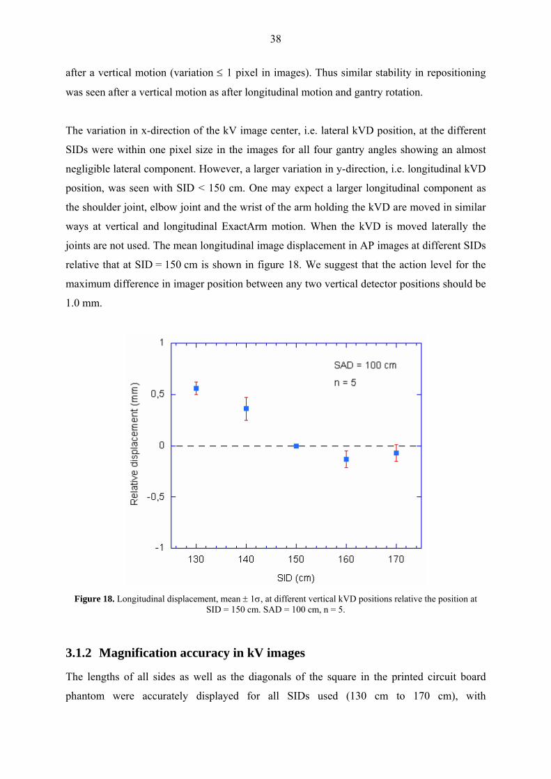
38

after a vertical motion (variation ≤ 1 pixel in images). Thus similar stability in repositioning

was seen after a vertical motion as after longitudinal motion and gantry rotation.

The variation in x-direction of the kV image center, i.e. lateral kVD position, at the different

SIDs were within one pixel size in the images for all four gantry angles showing an almost

negligible lateral component. However, a larger variation in y-direction, i.e. longitudinal kVD

position, was seen with SID < 150 cm. One may expect a larger longitudinal component as

the shoulder joint, elbow joint and the wrist of the arm holding the kVD are moved in similar

ways at vertical and longitudinal ExactArm motion. When the kVD is moved laterally the

joints are not used. The mean longitudinal image displacement in AP images at different SIDs

relative that at SID = 150 cm is shown in figure 18. We suggest that the action level for the

maximum difference in imager position between any two vertical detector positions should be

1.0 mm.

Figure 18. Longitudinal displacement, mean ± 1σ, at different vertical kVD positions relative the position at

SID = 150 cm. SAD = 100 cm, n = 5.

3.1.2 Magnification accuracy in kV images

The lengths of all sides as well as the diagonals of the square in the printed circuit board

phantom were accurately displayed for all SIDs used (130 cm to 170 cm), with

39

SSD = 100 cm, throughout the three months period. When the printed circuit board was

positioned at SSD = 110 cm and SSD = 90 cm the measured lengths of the sides of the square

were within ± 0.3 mm of the theoretical values calculated for beam divergence of a point

source; 90.9 mm and 111.1 mm for respective SSD.

In a QC this test can be performed together with the linearity of vertical detector arm motion

test (section 3.1.1.d). At each SID both the displacement of the graticule on the circuit board

and the sides of the square can be measured, see figure 19. We suggest that the tolerance level

of the measured lengths are < ± 0.5 mm relative the expected lengths at SSD between 90-110

cm.

Figure 19. A kV-image of the printed circuit board phantom. The sides of the 10×10 cm2 square are measured as well as the disagreement between the graticule on the circuit board and the digital graticule.

3.1.3 CBCT reconstruction center

The mean transverse vector displacement of the CBCT marker from the isocenter (reference

marker) as well as the mean lateral- and vertical components and the longitudinal

displacement of ten measurements are shown in table 4. The longitudinal accuracy was less in

the reconstructed CBCT images compared with kV images. The extension of the BB in the

longitudinal direction will depend on the slice width and be influenced by the small instability

during gantry rotation (figure 15, section 3.1.1.b). The accuracy when measuring a

longitudinal displacement is therefore less than when measuring a transverse displacement.

The mean vector displacement in transversal images agrees well with the mean amplitude of

40

the sine curves fitted to the measured x-displacements in kV images acquired over a gantry

rotation (section 3.1.1.b). This indicates agreement between the COR of the OBI and the

image center in transversal CBCT slices. In figure 20 the displacement of the BB in a

transversal CBCT slice is compared with the x-position in kV-images acquired over a gantry

rotation just prior to the CBCT scan. The position and magnitude of the amplitude of the fitted

sine curve agrees with the direction and magnitude of the vector displacement in the

transversal CBCT image. This test was performed three times and the agreement between

amplitude and transverse vector displacement was within 0.2 mm. When 3D/3D match is

performed the CBCT image is superimposed on the reference image so that the reconstructed

CBCT center coincides with the reference CT origin (planning isocenter). When a 2D/2D

match is performed the digital graticule is superimposed on the reference origin in the DRRs.

Thus the difference in accuracy in the transverse plane between 3D/3D and 2D/2D matches

will mainly depend on the lateral kVD offset, i.e. vertical shift of the sine curve.

No difference in CBCT isocenter was seen with the MVD extracted. Further, no difference in

the transversal image center was observed using half-fan compared with full-fan. However,

the extension of the BB in longitudinal direction differed slightly between the two acquisition

geometries.

Figure 20. The projected transverse displacement of the BB from the digital graticule over a gantry rotation (left) is compared with the displacement in a transversal CBCT image (right). The CBCT image in white and the reference CT in gray centered at treatment planning isocenter. The transverse CBCT center agrees well with the center-of-rotation, i.e. the vector displacement (RT) agrees with the amplitude of the fitted sine curve in both magnitude and direction. The kVD offset relative the kV beam axis increase the apparent displacement (relative digital graticule) in AP kV-images and decrease the apparent displacement in RL kV-images.

41

Table 4: Displacement of the BB in CBCT images showing the disagreement between CBCT isocenter and calibrated treatment isocenter, n = 10. RT = vector displacement in transversal image.

Mean displacement ± 1σ [mm]

RT Lat Vrt Lng

0.8 ± 0.2 0.3 ± 0.3 0.6 ± 0.2 0.8 ± 0.5

The CBCT center is compared with orthogonal kV and MV images in table 5. The

longitudinal displacement of the BB used for the kV and MV images is the mean of the

measured displacements in the AP and RL images. The difference in vertical and lateral

directions between CBCT and kV images agrees with the estimated lateral kVD offset. A

disagreement in longitudinal position was observed. The agreement in CBCT and MV image

center can be seen as the agreement between the CBCT center and the MV radiation isocenter

only if the MVD position is accurately calibrated.

Table 5: Mean absolute difference in position of the BB in CBCT images relative orthogonal kV- and MV-

images, n = 6. Mean disagreement ± 1σ [mm]

Lat Vrt Lng

⎪CBCT – kV⎪ 0.5 ± 0.1 0.5 ± 0.1 0.7 ± 0.4

⎪CBCT – MV⎪ 0.8 ± 0.3 0.1 ± 0.3 2.4 ± 0.6

3.2 IMAGE REGISTRATION AND COUCH SHIFT ACCURACY

3.2.1 2D/2D match application

3.2.1.a AP and RL kV images

All 2D/2D matches were performed manually as fiducial markers will in general be ignored

by automatic 2D/2D match since the registration algorithms are based on major anatomical

structures. The match applications works internally with 10th of millimeter precision, but the

displayed shift values are rounded off to integer millimeters. The couch shift values agreed

well with the distances measured with the measuring tool rounded of to nearest integer

millimeter. The disagreement between image displacement measured with the measuring tool

and the actual shifts are shown in the appendix. Table 6 shows the disagreement between the

42

displayed shift values and the actual phantom displacement for six different displacements.

The couch shift value for the mean longitudinal position in AP and RL images has been used. Table 6: Mean disagreement between the couch shift values given in the OBI application after 2D/2D matches

and the expected shifts, n = 12. Positive value in vertical, longitudinal and lateral directions means that the couch shift value disagrees with the actual shift in the anterior, inferior and right directions.

Actual shift Mean disagreement ± 1σ [mm]

Amount Direction Vrt Lngb Lat

S, P, R -0.3 ± 0.6 -0.1 ± 0.4 0.5 ± 0.6

20 mm I, A, L -0.5 ± 0.6 0.0 ± 0.2 1.0 ± 0.4

I, P, La 0.6 ± 0.5 -0.5 ± 0.6 1.3 ± 0.6

S, P, R -1.5 ± 0.6 -0.7 ± 0.6 -0.5 ± 0.6

35 mm I, A, L -1.0 ± 0.3 0.2 ± 0.3 0.0 ± 0.2

I, P, La 1.3 ± 0.6 1.0 ± 0.2 2.0 ± 0.5 Abbreviations: Vrt = vertical, Lng = longitudinal, Lat = lateral. a) n = 6. b) The longitudinal match is performed in between the BB position in the AP and RL images.

The difference in measured position of the BB in images acquired before and after the

phantom was shifted agreed very well with the actual shift corrected for beam divergence, see

appendix. The main factors determining the agreement between the displayed and the

expected values are thus the kV image center accuracy (section 3.1.1), beam divergence and

round off approximation. The effect of beam divergence depends on both magnitude and

direction of the shift. At certain phantom displacements this will reduce the apparent kV

image center offset and at other shifts it will increase the error. Thus the result of a 2D/2D

match is highly dependent on the direction of the displacement, e.g. compare lateral

disagreement (table 6) when the phantom is shifted 35 mm in the I, A and L directions (no

disagreement) and when the phantom is shifted 35 mm in the I, P and L directions

(error ∼ 2 mm).

At large shifts it may not be possible to match all markers accurately due to beam divergence.

Further, the longitudinal position of the BB may differ significantly in AP and RL images. In

figure 21 the relative difference in longitudinal position in AP and RL images is plotted as a

function of the magnitude of the phantom shift in P, S and R directions. In clinical practice, it

is therefore likely that at least one additional 2D/2D match is necessary to correct for a large

offset. In the second match the disagreement with the reference images will be much smaller

and the influence of beam divergence negligible, see figure 22. We suggest that an additional

2D/2D match is performed whenever any couch shift value > 2 cm.

43

The performance of the 2D/2D match was seen stable over the period of measurements.

Therefore, we conclude that it is not necessary to perform separate regular QC tests for the

2D/2D match application as long as the OBI isocenter agreement is regularly checked.

Figure 21. The mean difference in longitudinal position between AP and RL images as function of displacement

in the superior and posterior and right directions. When the phantom is in its initial position we see the small difference in longitudinal position observed previously, table 1.

(a) (b) Figure 22. (a) RL and AP kV-images (yellow) of the marker phantom shifted 3.5 cm in the S, P and R directions are matched with the reference images (blue). In the lower images the center marker has been zoomed in. Due to beam divergence a precise match of all markers cannot be performed and the markers cannot be matched in longitudinal direction in both the AP and the RL set simultaneously. (b) A second 2D/2D match after applied couch shift allows all markers to be matched adequately. The disagreement between the red and green graticule shows the inaccuracy of the first match.

44

3.2.1.b MV-MV and MV-kV images

The agreement in couch shift values when performing kV-kV, MV-MV and MV-kV 2D/2D

matches was consistent with the MV-kV image center disagreement, see section 3.1.1c. As

the couch shift values are rounded of to integer millimeters, disagreements of 2 mm in

longitudinal shift value in kV-kV and MV-MV match was frequently observed. As the

longitudinal position is seen both in AP and RL images the disagreement of about 1.5 mm

(section 3.1.1c) also complicated MV-kV matches even at small shifts. This was seen to be

the main disadvantage of MV-kV matches. MV-MV and MV-kV matches agreed better with

the expected shift in lateral direction than kV-kV matches. This is, however, a matter of

calibration of the MVD and the OBI ExactArms. If the OBI ExactArms are calibrated

correctly and regularly checked in a QA program there are no advantages to use MV-MV

match or MV-kV match compared with kV-kV match. MV-MV matching is much more time

consuming than kV-kV matching and is not as simple to perform due to inferior image

quality, especially when matching anatomical structures. When performing a MV-kV match it

is not necessary to rotate the gantry, still a MV image takes significantly longer time to

acquire and additional time to extract the MVD results in a longer overall matching time

compared with a kV-kV match. Further, MV images results in higher delivery doses to the

patient.

MV-kV match may be used in QA to verify agreement in longitudinal image position. More

generally MV AP and RL images should be compared with kV AP and RL images for image

center agreement.

3.2.1.c 2D/2D match with kV images acquired at oblique angles

It is possible to use other gantry orientations when performing 2D/2D match than orthogonal

image pairs. For orthogonal images, the two sets will be matched independently. However, at

other gantry angles than 0°, 90°, 180° and 270° the x-position will include both a lateral and

vertical component. With orthogonal images acquired at different gantry orientations the

match result will mainly depend on the kV image center agreement at those specific

orientations, see section 3.1.1b. For non-orthogonal matches performed with 60° to 120°

between the image pairs the disagreement in couch shift values with an AP-RL match was

≤ 1 mm. The registration time in this case is slightly longer as the two image sets are not

45

matched independently in x-direction, i.e. adjusting one image set affects the other image set

both in x- and y-direction. With smaller angles than 60° or larger than 120° between the

images pairs the matches were shown to be less accurate. Oblique setup fields may be used

clinically when no orthogonal treatment fields are used.

3.2.2 Marker Match application

Figure 23 shows a Marker Match of the Marker phantom displaced both translational and

rotational. When all the reference markers as well as all the markers in the kV images were

included in the region of interest (ROI) the automatic MarkerMatch application worked very

accurately. When using the Marker Match application each marker in the kV images is

matched independently with corresponding marker in the reference CT. Thus any

disagreement in longitudinal position in the AP and RL images or any distortion in relative

distances between the markers does not complicate the match procedure. Further, the Marker

Match application was seen to correct for inaccurate distance magnification due to beam

divergence and hence be less dependent on the magnitude of the shift than 2D/2D match.

However, it is difficult to tell the accuracy of this correction as the couch shift values are

rounded of to nearest integer millimeter. In table 7 translational couch shift values with

Marker Match are compared with the actual phantom displacements and the couch shift

values when using 2D/2D match. The Marker phantom was shifted 2.0 cm and 3.5 cm both in

S, P and R directions and in I, A and L directions. The mean error agree well with the

estimated image center off-set, section 3.1.1. The difference in couch shift values with Marker

Match and 2D/2D agrees reasonable well with the error in image magnification in the kV

images. Thus, Marker Match is more accurate at large displacements, ≥ 20 mm.

46

Figure 23. The automatic Marker Match application is used to correct the position of the marker phantom after a translational and a rotational (seen in the AP images) displacement. (a) The detected reference markers are displayed as red digital cross-marks on the orthogonal kV-images. (b) The digital cross-marks are matched with the markers in the kV-images and become green. The region of interest is displayed in red.

Further, Marker Match application was seen to correct more accurately for rotational shifts.

The agreement of the rotational shift value and the expected couch rotation agreed within 0.3°

for rotations up to 10° in both directions (clockwise and counterclockwise). This includes a

set-up error. We estimated the accuracy to be better than 0.2°, both when correcting only for

angular displacement and when correcting for combined angular and translational

displacement. However, the system does not allow applying mechanical couch rotations larger

than 4°- 6°, depending on lateral couch position. Compared with 2D/2D match, the Marker

Match application was significantly more stable and precise in its performance at large couch

rotations, ≥ 2°, and with combined translational and rotational shifts. In clinical practice

however, rotational errors in patient position is not as common as translational errors. If the

tumor it self is rotated it is a question whether a correction for this error will give a more

accurate dose delivery than if not corrected for. If the tumor is spherical symmetric a

rotational couch shift will not improve the target position, while this will change the position

of surrounding organs and bony structures relative the treatment fields and may lead to an

inadequate dose delivery. Further, rotation around the AP axis may not be the most likely

direction of rotation of the tumor, e.g. the prostate is seen to more commonly rotate around

the LR axis depending on rectum and bladder filling (Boer et al 2005).

47

Another advantage of Marker Match is that the result is independent of the performance of the

user. Further, our 2D/2D match results may be overestimated compared with the accuracy in

clinical practice as the center BB was placed in origin and then the digital graticule was used

for a precise image match. When adjusting the origin to coincide with the center BB in the

reference CT the generated DRRs may still not be centered at the origin. The pixel size in the

DRRs are 1 mm and as the graticule cannot be centered in a pixel the center BB was displaced

0.5 mm in all directions, relative the reference graticule, in our DRRs. Thus if the 2D/2D

matches are performed with the actual reference image instead of the graticule an additional

error is introduced. MarkerMatch does not have this problem as the match is performed with

the reference CT which was accurately centered at the user origin.

We suggest that one uses the automatic match application instead of manual matching as it is

less time consuming. It is however important to always check the results of both the automatic

detection and the automatic match by zooming in on the markers and, if necessary, make

minor adjustments. We found the MarkerMatch application to be very efficient and with

correct calibration of the kVS and kVD this application gives very accurate and stable results.

MarkerMatch is the most adequate application when gold markers are implanted and should

be the preferred method to use clinically instead of 2D/2D match, which is mainly used now,

for more accurate and user independent results. The only disadvantage is that for smaller

corrections a Marker Match takes up to half a minute longer time than a 2D/2D match. The

marked reference CT cannot be saved until subsequent sessions and the whole procedure of

detecting the markers must be repeated at each treatment fraction. Therefore 2D/2D match

may still be used at small positional errors to save time.

Table 7: Absolute difference between the translational couch shift values when using Marker Match and (a) the

actual shift and (b) the couch shift values using 2D/2D match, n = 12. Relative actual shift, Mean ± 1σ [mm]

(a) Vrt Lng Lat

20 mm shift 0.0 ± 0.0 0.0 ± 0.0 1.0 ± 0.0

35 mm shift 0.2 ± 0.4 0.0 ± 0.0 0.8 ± 0.5

Relative 2D/2D match, Mean ± 1σ [mm]

(b) Vrt Lng Lat

20 mm shift 0.5 ± 0.6 0.0 ± 0.0 0.5 ± 0.6

35 mm shift 1.5 ± 0.6 0.6 ± 0.6 1.3 ± 0.4 Abbreviations: Vrt = vertical, Lng = longitudinal, Lat = lateral.

48

3.2.3 3D/3D match application

The image magnification in transversal CBCT slices was seen to be very accurate, see section

3.3.2, and the couch shift values agreed well with the measured distances rounded off to

nearest integer mm. The accuracy of 3D/3D match mainly seemed to be limited by the

agreement between the reconstructed CBCT center and the treatment isocenter discussed in

section 3.1.3. The accuracy in longitudinal match also depends on the slice width. Table 8

shows the mean disagreement in translational couch shift values between 3D/3D and 2D/3D

matches. The Marker phantom was shifted 2.0 cm and 3.5 cm both in S, P and R directions

and in I, A and L directions. Even though the relative values are influenced by round of errors

the difference in match results agrees reasonable well with the difference in kV image center

for AP and RL images and the CBCT reconstruction center, see section 3.1.3. In table A3 in

appendix the residual error of the three match applications are shown for the same phantom

setups.

3D/3D matches were most difficult to perform when correcting for rotational shifts. With

implanted markers we found no advantages to use 3D/3D match over Marker Match. The time

to perform a 3D/3D match is about 10 minutes compared with approximately 1 minute for

Marker Match. Further, the time span to perform 3D/3D match may result in intra-fractional

motion of the tumor. When matching anatomical structures CBCT images reveal soft tissue

contrast superior to that of kV images, less tissue overlapping and accurate image

magnification (section 3.3.2). Automatic 3D/3D match for translational shifts with an

anthropomorphic phantom have previously been tested in the institution showing adequate

results. Automatic match with rotational shifts should be further investigated.

Table 8: Mean difference in couch shift values

between 3D/3D and 2D/3D match, n = 12. Mean difference ± 1σ [mm]

Vrt Lng Lat

0.4 ± 0.6 0.8 ± 0.6 0.6 ± 0.6 Abbreviations: Vrt = vertical, Lng = longitudinal, Lat = lateral.

3.2.4 Physical couch shift

The agreement between measured mechanical couch shift and the displayed shift values was

within 1 mm. No clear systematic disagreement between the actual shift of the couch and the

49

couch shift values generated by the OBI applications was observed in any couch direction.

Further no dependence on the magnitude of the shift was seen. In table 9 the mean difference

between translational couch shift values and the physical couch shift are shown. Small lateral

and longitudinal components were notified at a few occasions when rotational couch shifts of

2° or more were applied. Uncertainties in the couch shift, and round of errors in the OBI

applications, and in the OBI isocenter agreement limits the expected accuracy of a couch

correction to < 1 mm. In clinical practice we therefore suggest that couch shift is only applied

whenever any couch shift value is greater than 1 mm.

Table 9: Disagreement between physical couch shift and displayed shift values, n = 16. Positive value means that the measured couch shift is larger than the displayed value.

Mean disagreement ± 1σ [mm]

Vrt Lng Lat

0.1 ± 0.6 0.0 ± 0.5 -0.2 ± 0.6 Abbreviations: Vrt = vertical, Lng = longitudinal, Lat = lateral.

3.3 IMAGE QA

3.3.1 kV image quality

With the x-ray technique used 16 (2.3%) to 17 (3.1%) contrast disks were discernible in the

N3 phantom. The bar pattern in the 10th group was discernible in the Huttner 18 phantom

which corresponds to 1.8 lp/mm. kV images of the phantoms are shown in figure 24 (a) and

(b). The main concern in image quality QA is the consistency in image quality performance

over time. Routine checks have to be performed as with any other radiological equipment. In

the Leeds series there are two phantoms recommended for routine tests of both spatial

resolution and contrast resolution; TOR [CDR] and TOR [18 FG], [Leads Test Objects

Information Pack (North Yorkshire, UK, Leeds Test Objects Ltd,

www.leedstestobjects.com.)] Both phantoms contain a line pair test, analogous to the Huttner

phantom, and 18 contrast discs. TOR [CDR] contains an additional detail test with 10 test

points and is recommended for digital radiography. TOR [18 FG] contains two additional

circular geometry test objects and is primarily recommended for monitoring of fluoroscopic

images. However, due to the similarity of the two phantoms the TOR [18 FG] may be used for

both the fluoroscopic mode and the radiographic mode. A radiographic image of TOR [18

FG] is shown in figure 24 (c).

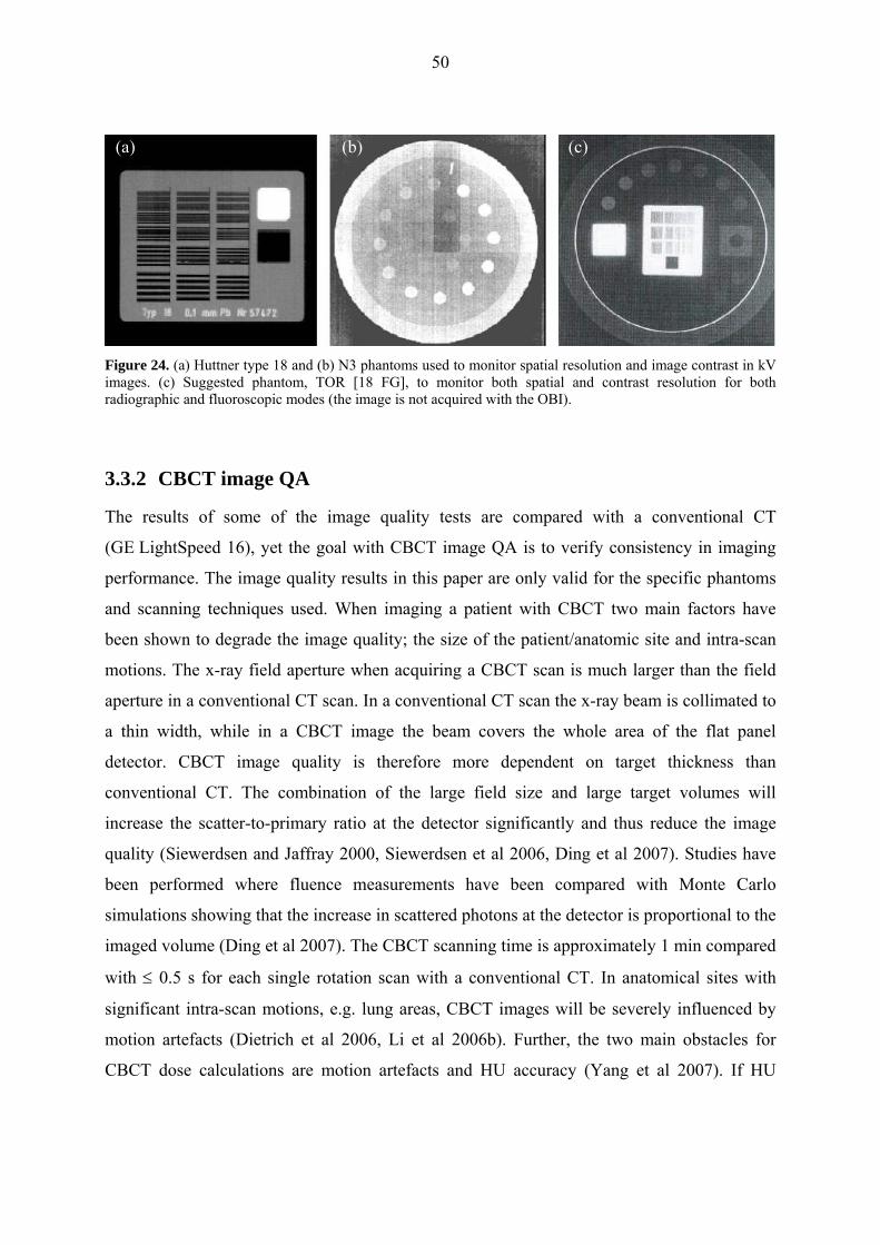
50

(a) (b) (c)

Figure 24. (a) Huttner type 18 and (b) N3 phantoms used to monitor spatial resolution and image contrast in kV images. (c) Suggested phantom, TOR [18 FG], to monitor both spatial and contrast resolution for both radiographic and fluoroscopic modes (the image is not acquired with the OBI).

3.3.2 CBCT image QA

The results of some of the image quality tests are compared with a conventional CT

(GE LightSpeed 16), yet the goal with CBCT image QA is to verify consistency in imaging

performance. The image quality results in this paper are only valid for the specific phantoms

and scanning techniques used. When imaging a patient with CBCT two main factors have

been shown to degrade the image quality; the size of the patient/anatomic site and intra-scan

motions. The x-ray field aperture when acquiring a CBCT scan is much larger than the field

aperture in a conventional CT scan. In a conventional CT scan the x-ray beam is collimated to

a thin width, while in a CBCT image the beam covers the whole area of the flat panel

detector. CBCT image quality is therefore more dependent on target thickness than

conventional CT. The combination of the large field size and large target volumes will

increase the scatter-to-primary ratio at the detector significantly and thus reduce the image

quality (Siewerdsen and Jaffray 2000, Siewerdsen et al 2006, Ding et al 2007). Studies have

been performed where fluence measurements have been compared with Monte Carlo

simulations showing that the increase in scattered photons at the detector is proportional to the

imaged volume (Ding et al 2007). The CBCT scanning time is approximately 1 min compared

with ≤ 0.5 s for each single rotation scan with a conventional CT. In anatomical sites with

significant intra-scan motions, e.g. lung areas, CBCT images will be severely influenced by

motion artefacts (Dietrich et al 2006, Li et al 2006b). Further, the two main obstacles for

CBCT dose calculations are motion artefacts and HU accuracy (Yang et al 2007). If HU

51

accuracy is achieved accurate dose calculations should at least be possible for sites with low

intra-scan motions, e.g. prostate treatments.

3.3.2.a HU uniformity and stability

The mean HU values in the five ROIs for seven measurements with full-fan and half-fan are

presented in table 10. The values are also compared with one measurement in a conventional

CT image. Images acquired with FF mode showed good in-slice uniformity; variation

between ROIs < 5 HU in all but one measurement. For FF mode the mean values of the

different ROIs are within the expected for the material (0 ± 20 HU) and within 5 HU of the

planning CT values. The mean spatial uniformity, as defined in equation (2), was 0.3 % for

full-fan images and 6.7 % for half-fan images. In figure 25(a) the mean of the mean values in

the five ROIs are plotted against date of measurement to evaluate the HU stability. In

figure 25(b) the spatial uniformity is plotted for the same measurements. In the first

measurement with FF geometry the phantom was somewhat tilted in forward direction

resulting in larger HU values but still the same uniformity. For the measurements with the

phantom positioned correctly the variation in mean ROI value from measurement to

measurement was < ± 5 HU with FF mode.

With HF mode differences up to ~ 70 HU was seen between the ROIs. The center ROI

showed a lower HU value and a decrease in HU values was seen diagonally from upper-left to

lower-right in the image, which can be seen with line profiles, see figure 26. The lower HU

values towards the center of the phantom may be explained by inaccurate beam hardening

corrections, i.e. cupping artifacts. After recalibration of the HF mode, the HU values in the

peripheral ROIs agreed better with the central ROI, still a diagonal variation was seen. The

HF mode is calibrated with a larger homogeneous phantom approximating the size of an

average pelvis. However, a large non-uniformity was observed when using RMI phantom;

maximum variation between ROIs ∼ ± 120 HU. When the HU uniformity was measured again

with the Catphan phantom two months later the non-uniformity had increased with HF mode.

This indicates that regular QA tests and norm calibrations of the CBCT has to be performed,

especially with HF mode. Nevertheless, both with FF mode and HF mode the variation

between the ROIs, using the Catphan phantom, were within ± 40 HU. The inter-slice variation

was < 5 HU with FF mode and < 10 HU with HF mode in all measurements.

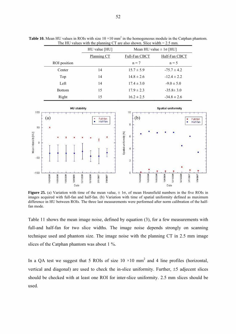
52

Table 10. Mean HU values in ROIs with size 10 ×10 mm2 in the homogeneous module in the Catphan phantom.

The HU values with the planning CT are also shown. Slice width = 2.5 mm. HU value [HU] Mean HU value ± 1σ [HU]

Planning CT Full-Fan CBCT Half-Fan CBCT

ROI position n = 7 n = 5

Center 14 15.7 ± 5.9 -75.7 ± 4.2

Top 14 14.8 ± 2.6 -12.4 ± 2.2

Left 14 17.4 ± 3.0 -9.0 ± 5.0

Bottom 15 17.9 ± 2.3 -35.8± 3.0

Right 15 16.2 ± 2.5 -34.8 ± 2.6

(a) (b)

Figure 25. (a) Variation with time of the mean value, ± 1σ, of mean Hounsfield numbers in the five ROIs in images acquired with full-fan and half-fan. (b) Variation with time of spatial uniformity defined as maximum difference in HU between ROIs. The three last measurements were performed after norm calibration of the half-fan mode.

Table 11 shows the mean image noise, defined by equation (3), for a few measurements with

full-and half-fan for two slice widths. The image noise depends strongly on scanning

technique used and phantom size. The image noise with the planning CT in 2.5 mm image

slices of the Catphan phantom was about 1 %.

In a QA test we suggest that 5 ROIs of size 10 ×10 mm2 and 4 line profiles (horizontal,

vertical and diagonal) are used to check the in-slice uniformity. Further, ±5 adjecent slices

should be checked with at least one ROI for inter-slice uniformity. 2.5 mm slices should be

used.

53

Table 11. Mean image noise, n = 4. The mean of the standard deviations in the five ROIs have been used in each measurement.

Mean image noise ± 1σ (%)

Slice width Full-fan Half-fan

1.0 mm 1.5 ± 0.2 1.7 ± 0.2

2,5 mm 1.0 ± 0.1 1.2 ± 0.2

Figure 26. HU profiles of images of the homogeneous module in the Catphan phantom. (a) The direction of the line profiles in; (b) planning CT, (c) full-fan mode CBCT and (d) half-fan mode CBCT.

(a) (b)

(c) (d)

3.3.2.b HU Linearity

The mean HU values for the different materials in CBCT images acquired with full-and half-

fan are shown in table 12. The HU values for one measurement in a conventional CT image

are also shown. In figure 27 the mean HU values are plotted against the expected values. The

measured HU values for FF mode agreed with the expected values within the required limit

(± 40 HU) except for Teflon, which disagreed with approximately 160 HU. This indicates

54

inaccuracy in HU values in the high density region comparable with that of bone

(~ 1000 HU). Further, the agreement with the planning CT was good below zero HU. Above

zero the gradient is steeper than in the planning CT and for Teflon the disagreement was

> 200 HU. With HF mode only the three lowest density targets agreed within the expected

limit. The measured values with HF mode will also be influenced by non-uniformity, see

section 3.3.2.a. However, the HF mode agreed better with the planning CT, seen over the

whole region. FF mode agreed better in the region -200 HU to 340 HU, equivalent to soft

tissue; fat about -120 to -20 HU and muscle about 40 HU. Agreement between HU density

and electron density of the medium is crucial for dose verification with the CBCT. However,

our measurements indicate that for body scans with HF mode the HU non-uniformity seems

to be a greater problem. For overall agreement the same treatment plan can be applied on

planning CT and CBCT image of an anthropomorphic phantom. In figure 28 the deviation of

measured HU from the expected values are plotted against time for four of the targets.

Figure 27. Measured HU versus expected HU for planning CT, full-fan and half-fan mode CBCT. Mean HU are used for the CBCT modes, n = 6.

55

Table 12. Mean HU values in different materials are compared with the expected values and with planning CT, n = 6, ROI size = 5×5 mm2.

Material HU value [HU] Mean HU ± 1σ [HU]

Expected Planning CT Full-Fan CBCT Half-Fan CBCT

Air -1000 -960 -999.1 ± 0.3 -967.9 ± 3.4

PMP -200 -177 -186.0 ± 1.7 -202.9 ± 4.2

LDPE -100 -86 -87.5 ± 2.4 -110.3 ± 6.9

Polystryrene -35 -31 -28.6 ± 3.1 -79.1 ± 3.7

Acrylic 120 121 81.8 ± 4.1 61.7 ± 5.3

Delrin 340 338 372.2 ± 2.8 285.3 ± 6.4

Teflon 990 920 1153.5 ± 6.2 892.6 ± 7.6

(a) (b)

Figure 28. Long term stability of HU values; deviation in HU from expected value is plotted against time for air, LDPE, Acrylic and Teflon in (a) full-fan and (b) half-fan images.

3.3.2.c In-slice Geometry

The measured distances between the holes ranged from 49.8 mm to 50.0 mm with FF, and

from 49.5 mm to 49.7 mm with the HF. Thus, the image magnification was slightly less exact

with HF geometry. However, the measurements of the diameter of the inner cylinder showed

better results with HF than with FF. This may be explained by reduced accuracy in the

measurements due to blurred edges on the upper-left and lower-right sides of the cylinder in

images acquired with FF, see figure 31. The reason for this blurriness should be investigated.

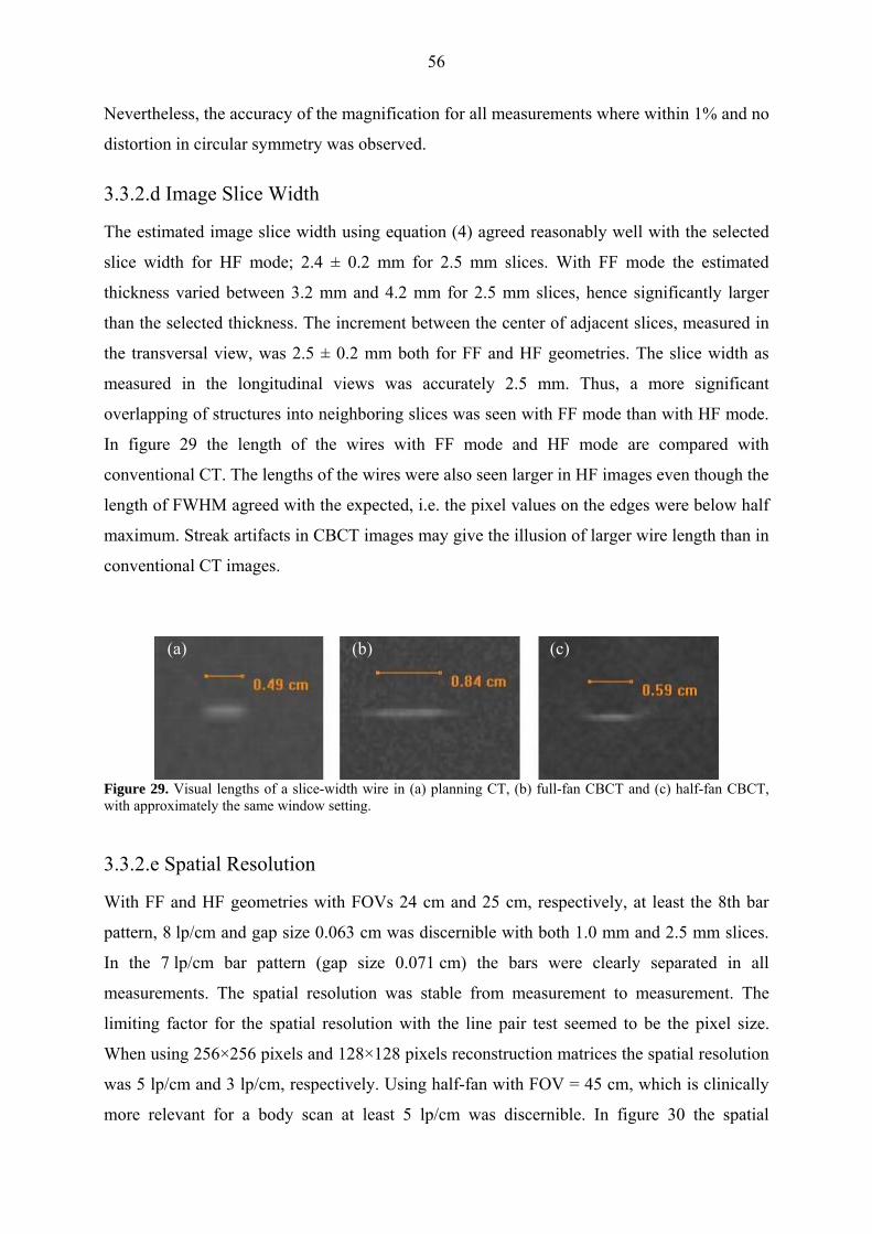
56

Nevertheless, the accuracy of the magnification for all measurements where within 1% and no

distortion in circular symmetry was observed.

3.3.2.d Image Slice Width

The estimated image slice width using equation (4) agreed reasonably well with the selected

slice width for HF mode; 2.4 ± 0.2 mm for 2.5 mm slices. With FF mode the estimated

thickness varied between 3.2 mm and 4.2 mm for 2.5 mm slices, hence significantly larger

than the selected thickness. The increment between the center of adjacent slices, measured in

the transversal view, was 2.5 ± 0.2 mm both for FF and HF geometries. The slice width as

measured in the longitudinal views was accurately 2.5 mm. Thus, a more significant

overlapping of structures into neighboring slices was seen with FF mode than with HF mode.

In figure 29 the length of the wires with FF mode and HF mode are compared with

conventional CT. The lengths of the wires were also seen larger in HF images even though the

length of FWHM agreed with the expected, i.e. the pixel values on the edges were below half

maximum. Streak artifacts in CBCT images may give the illusion of larger wire length than in

conventional CT images.

(a) (b) (c)

Figure 29. Visual lengths of a slice-width wire in (a) planning CT, (b) full-fan CBCT and (c) half-fan CBCT, with approximately the same window setting.

3.3.2.e Spatial Resolution

With FF and HF geometries with FOVs 24 cm and 25 cm, respectively, at least the 8th bar

pattern, 8 lp/cm and gap size 0.063 cm was discernible with both 1.0 mm and 2.5 mm slices.

In the 7 lp/cm bar pattern (gap size 0.071 cm) the bars were clearly separated in all

measurements. The spatial resolution was stable from measurement to measurement. The

limiting factor for the spatial resolution with the line pair test seemed to be the pixel size.

When using 256×256 pixels and 128×128 pixels reconstruction matrices the spatial resolution

was 5 lp/cm and 3 lp/cm, respectively. Using half-fan with FOV = 45 cm, which is clinically

more relevant for a body scan at least 5 lp/cm was discernible. In figure 30 the spatial

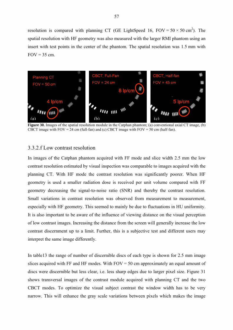
57

resolution is compared with planning CT (GE LightSpeed 16, FOV = 50 × 50 cm2). The

spatial resolution with HF geometry was also measured with the larger RMI phantom using an

insert with test points in the center of the phantom. The spatial resolution was 1.5 mm with

FOV = 35 cm.

(a) (b) (c)Figure 30. Images of the spatial resolution module in the Catphan phantom; (a) conventional axial CT image, (b) CBCT image with FOV = 24 cm (full-fan) and (c) CBCT image with FOV = 50 cm (half-fan).

3.3.2.f Low contrast resolution

In images of the Catphan phantom acquired with FF mode and slice width 2.5 mm the low

contrast resolution estimated by visual inspection was comparable to images acquired with the

planning CT. With HF mode the contrast resolution was significantly poorer. When HF

geometry is used a smaller radiation dose is received per unit volume compared with FF

geometry decreasing the signal-to-noise ratio (SNR) and thereby the contrast resolution.

Small variations in contrast resolution was observed from measurement to measurement,

especially with HF geometry. This seemed to mainly be due to fluctuations in HU uniformity.

It is also important to be aware of the influence of viewing distance on the visual perception

of low contrast images. Increasing the distance from the screen will generally increase the low

contrast discernment up to a limit. Further, this is a subjective test and different users may

interpret the same image differently.

In table13 the range of number of discernible discs of each type is shown for 2.5 mm image

slices acquired with FF and HF modes. With FOV = 50 cm approximately an equal amount of

discs were discernible but less clear, i.e. less sharp edges due to larger pixel size. Figure 31

shows transversal images of the contrast module acquired with planning CT and the two

CBCT modes. To optimize the visual subject contrast the window width has to be very

narrow. This will enhance the gray scale variations between pixels which makes the image

58

look noisier. The low contrast resolution is highly dependent on the slice thickness. Larger

slice thickness uses more photons to produce the image and thereby increase the SNR and

hence also the contrast resolution. Twice the slice thickness will use approximately twice as

many photons increasing the SNR by a factor 2 . With slice thickness 1 mm reduced contrast

resolution was seen with both FF and HF mode compared with 2.5 mm slices. With FF mode

2 to 4 of the 1.0 % supra-slice contrast discs and none of the 0.5 % contrast discs were

discernible.

Table 13. Number of discernible discs in the Catphan low contrast module. Slice width = 2.5 mm.

# discernible discs

Disc type Full-Fan Half-Fan

1.0 % Supra-slice 5 - 7 4 - 5

0.5 % Supra-slice 3 - 6 0

0.3 % Supra-slice 0 0

7 mm Sub-slice 2 - 4 1 - 2

5 mm Sub-slice 1 - 3 0

3 mm Sub-slice 0 - 1 0

To estimate the actual subject contrast of the targets with nominal contrast of 1.0 % we

measured the HU in a ROI covering most of the largest disc and in ROIs in the surrounding

background. This was done in several scans and the mean value of the estimated subject

contrast was 1.0 ± 0.2 %. The contrast resolution test with the Catphan phantom is for QA

only and not a test for subject contrast in general. To estimate the contrast resolution in a body

scan more scattering material should be used for HF geometry. The contrast resolution in

CBCT images is much more dependent on patient size than conventional CT due to a larger

increase in SPR. In an anatomic image the contrast resolution will not only be influenced by

quantum noise but also by structure noise.

59

(a) (b) Planning CT

(c) Full-Fan CBCT (d) Half-Fan CBCT

Figure 31: Images of low contrast module (a) in Catphan 504 phantom; (b) planning CT (GE LightSpeed 16), (c) full-fan CBCT and (d) half-fan CBCT. Slice-thickness = 2.5 mm. The images look noisy as the window width is set narrow to increase contrast resolution.

60

4 CONCLUSIONS In this project different tests were performed to evaluate the performance of an On-Board

Imager® (OBI) mounted on a clinical linear accelerator. The measurements were divided into

three parts; geometric accuracy, image registration and image quality. Tests to verify the

geometric accuracy are the most critical and have to be performed regularly. Our

measurements showed mechanical stability of the OBI over a 3-month period. The ExactArms

were seen to be stable during gantry rotation as well as in reproducing position after

longitudinal and vertical arm motions. However, the isocentric setup of the OBI was seen not

to be optimal during the test period. Small disagreements between the three imaging systems;

MV-, kV and CBCT, were observed. The difference between the transversal kV-image and

CBCT center was shown to depend on a small lateral detector offset. Accuracy in the

agreement with treatment isocenter is however a matter of accurate calibration of source and

detector positions. This work shows the importance of regular geometric QC to detect any

deficiency and to maintain a desirable precision. Therefore, initially the frequency of

geometric tests has to be high until confidence is gained. A simple cube phantom containing

one radio opaque marker can be used for easy, fast and reliable tests to verify image center

accuracy for both kV and CBCT imaging.

A marker seed phantom was used to evaluate and compare the accuracy in image registration

with the different match applications supplied by the OBI system. Marker Match application

(2D/3D) was seen to correct more accurately than 2D/2D match at large translational and

rotational displacements. However, at smaller shifts (< 20 mm) the registration time with

2D/2D match is slightly shorter. Further, it is questionable if rotational couch correction for

tumor rotation will lead to improved dose delivery. 2D/2D matches were performed with both

kV- and MV-images. With regular geometric QC of the OBI we found no advantages in using

MV-MV or MV-kV match over kV-kV match. The kV-kV image registration is more

efficient, easier to perform, has better image quality and gives lower patient dose. The match

applications worked sufficiently and no irregularities were observed over a 3-month period.

Therefore, we do not find it necessary to perform regular QC of the match applications, as

long as frequent tests verifying geometric accuracy are performed. Even with an accurate

setup of the OBI the accuracy in a position correction is limited by a round-off approximation

and limitations in physical couch movement. We therefore suggest that couch shift is applied

only in directions where the displayed shift value is > 1 mm.

61

CBCT image quality and HU accuracy was evaluated using a Catphan phantom. The spatial

resolution and image contrast in CBCT images acquired with full-fan mode was comparable

to a conventional CT. However, overlapping of structures was observed when estimating the

slice thickness. Further, streak and dark band artefacts at low and high density interfaces are

more prominent than in conventional CT images. Half-fan images showed lower contrast

resolution than full-fan images. The image quality is further degraded when using larger

target sizes due to a significant increase in scattered photons. Full-fan CBCT images showed

good HU uniformity while half-fan images were less uniform. The HU agreement with

planning CT was quite good in the soft tissue region with full-fan geometry, but a larger

disagreement was observed at higher densities, similar to bone. QC of HU is necessary if the

CBCT mode will be evaluated further for off-line adaptive radiation therapy. In this case the

stability and consistency with the planning CT is crucial. To evaluate the use of the CBCT in

ART the same treatment plan should be applied on both CBCT and planning CT images of an

anthropomorphic phantom. An important aspect of ART is that the total time to perform

3D/3D image registration should be reduced to 3-5 minutes to avoid intra-fraction target

motion.

This work shows that the OBI is precise and stable in its performance. A geometric precision

of the OBI within 1 mm can be achieved and maintained with regular QC and re-calibrations.

62

ACKNOWLEDGEMENTS First and most I would like to thank my supervisor Dr. Bruno Sorcini for giving me the

opportunity to work with this interesting project at the Radiotherapy department at the

Karolinska University Hospital. Thanks for introducing me to the latest technology, learning

me about the treatment planning procedure and all good advices. Further, I would like to

thank the nurses in treatment room 5 for their kindness. I would also like to thank the

engineers that have helped me when I have got stuck with technical complications. Thanks to

the diagnostic radiology department for letting me borrow image quality phantoms. Last but

not least I would like to thank my gorgeous wife Isa Gumrin and my wonderful children

Alicia and Elis for all their support and comfort through this work.

63

REFERENCES Balter J M, Sandler H M, Lam K, Bree R L, Lichter A S and Ten Haken R K 1995

Measurements of prostate movement over the course of routine radiotherapy using implanted markers Int. J Radiat. Oncol. Biol. Phys. 31 113-18

Boer H C, Os M J, Jansen P P and Heijmen B J 2005 Application of the no action level (NAL) protocol to correct for prostate motion based on electric portal imaging of implanted markers Int. J. Radiat. Oncol. Biol. Phys. 65 963-83

Bushberg JT, Seibert JA, Leidholdt EM and Boone JM 2002 The Essential Physics of Medical Imaging, 2nd edition, chapter 13, ISBN 0-683-301 18-7, Lippincott Williams & Wilkins

Ding GX, Dugan DM and Coffey CW 2007 Characteristics of kilovoltage x-ray beams used for cone-beam computed tomography in radiation therapy Phys. Med. Biol. 52 1595-615

Dietrich L, Jetter S, Tucking T, Nill S and Oelfke U 2006 Linac-integrated 4D-cone beam CT: first experimental results Phys. Med. Biol. 51 2939-52

Dong H, Hammoud R, Li S, Chen Q, and Guan H 2006 The Hounsfield Unit (HU) accuracy in Varian's cone-beam CT (CBCT) and its effect on dosimetric verification Med. Phys. 33 2049

Hector C L, Webb S and Evans P M 2000 The dosimetric consequences of inter-fractional patient movement on conventional and intensity-modulated breast radiotherapy treatments Radiother. Oncol. 54 57-64

ICRU report 50 1993 Prescribing, recording, and reporting photon beam therapy Bethesda, Maryland, U.S.A.: International Commission on Radiation Units and Measurements

ICRU report 62 1999 Prescribing, recording, and reporting photon beam therapy (Supplement to ICRU report 50). Bethesda, Maryland, U.S.A.: International Commission on Radiation Units and Measurements

Jaffray DA, Drake DG, Moreau M, Martinez AA and Wong JW 1999 A radiographic and tomographic imaging system integrated into a medical linear accelerator for localization of bone and soft tissue targets Int. J. Radiat. Oncol. Biol. Phys. 45 773-89

Jaffray DA and Siewerdsen JH 2000 Cone beam computed tomography with a flat-panel imager: Initial performance characterization Med. Phys. 27 1311-23

Jaffray D A, Siewerdsen J H, Wong J W and Martinez A A 2002 Flat-panel cone-beam computed tomography for image guided radiation therapy Int. J. Radiat. Oncol. Biol. Phys. 53 1337-49

Létourneau D, Wong J W, Oldham M, Gulam M, Watt L, Jaffray D A, Siewerdsen J H and Martinez A A 2005 Cone-beam-CT guided radiation therapy: technical implementation Radiother. Oncol. 75 279-86

Li T, Schreibmann E, Yang Y and Xing L 2006a Motion correction for improved target localization with on-board cone-beam computed tomography Phys. Med. Biol. 51 253-67

Li T, Xing L, Munro P, McGuiness C, Yang Y, Cao M, Loo B and Kong A 2006b Four-dimensional cone-beam computed tomography using an on-board imager Med. Phys. 33 3825-33

Lo T, Yang Y, Schreibmann E, Li T and Xing L 2005 Mapping electron density distribution from planning CT to cone-beam CT (CBCT): A novel strategy for accurate dose calculation based on CBCT Int. J. Radiat. Oncol. Biol. Phys. Suppl. 63 S507

Mackie T R et al 2003 Image guidance for precise conformal radiotherapy Int. J. Radiat. Oncol. Biol. Phys. 56 89-105

64

Martinez A A et al 2001 Improvement in dose escalation using the process of adaptive radiotherapy combined with three-dimensional conformal or intensity modulated beams for prostate cancer Int. J. Radiat. Oncol. Biol. Phys. 50 1226-34

McBain C A et al 2006 X-ray volumetric imaging in image-guided radiotherapy: the new standard in on-treatment imaging Int. J. Radiat. Oncol. Biol. Phys. 64 625-34

Mohan R et al 2005 Use of deformed intensity distributions for on-line modification image-guided IMRT to account for inter-fractional anatomic changes Int. J. Radiat. Oncol. Biol. Phys. 61 1258-66

Oldham M, Létourneau D, Watt L, Hugo G, Yan D, Lockman D, Kim L H, Chen P Y, Martinez A A and Wong J W 2005 Cone-beam-CT guided radiation therapy: A model for on-line application Radiother. Oncol. 75 271-8

Parker R P, Hobday P A and Cassel K J 1979 The direct use of CT numbers in radiotherapy dosage calculations for inhomogeneous media Phys. Med. Biol. 24 802-9

Podgorsak E B 2003 Review of radiation oncology physics: A handbook for teachers and students. Educational reports series: IAEA

Sage J, Cullingford A, Dagless M, Kilby W, Hutchings R and Thomson E 1998 A complete program of CT quality assurance for radiotherapy treatment planning. IPEM annual conference, Brighton

Schewe JE, Lam KL, Balter JM and Ten Haken RK 1998 A room-based diagnostic imaging system for measurement of patient setup Med. Phys. 25 2385-7

Siewerdsen J H and Jaffray D A 2000 Cone-beam computed tomography with a flat-panel imager: Magnitude and effects of x-ray scatter Med. Phys. 28 220-31

Siewerdsen J H, Daly M, Bakhtiar B, Moseley D J, Richard S, Keller H and Jaffray D A 2006 A simple, direct method for x-ray scatter estimation and correction in digital radiography and cone-beam CT Med. Phys. 33 87-97

Sorcini B and Tilikidis A 2006 Clinical application of image-guided radiotherapy, IGRT (on the Varian OBI platform) Cancer Radiother. 10 252-7

Sorcini B 2006 Clinical introduction of image-guided radiation therapy and cone-beam computed tomography European Oncological Disease Issue 1 43-44

Webb S 2006 Motion effects in (intensity modulated) radiation therapy: a review Phys. Med. Biol. 51 R403-25

Xing L et al 2006 On-board volumetric CT-based adaptive IMRT for improved prostate cancer treatment Int. J. Radiat. Oncol. Biol. Phys. Suppl. 66 S624

Yang Y, Schreibmann E, Li T, Wang C and Xing L 2007 Evaluation of on-board kV cone beam CT (CBCT) – based dose calculations Phys. Med. Biol. 52 685-705

Yoo S et al 2006 A quality assurance program for the on-board imager Med. Phys. 33 4431-47

Zelefsky M J et al 2002 High dose intensity modulated radiation therapy for prostate cancer: Early toxicity and biochemical outcome in 772 patients Int. J. Radiat. Oncol. Biol. Phys. 53 1111-6

65

APPENDIX The couch shift values displayed at image registration are rounded off to integer millimeter.

With the measuring tool in the OBI application the distance between acquired image and

reference image can be measured with 10th of millimeter precision. For the same

displacements of the Marker phantom as in table 6, section 3.2.1, the distances between the

reference images and acquired kV-images were measured before matching. Table A1 shows

the disagreement between the measured distance, between the BB in acquired kV-images and

in reference images, Rshifted, and the actual phantom displacement. Table A2(a) shows the

absolute difference in position in images acquired before and after the phantom was shifted,

⎪Rshifted – Rinitial⎪, relative the theoretical shift corrected for beam divergence. Table A2(b)

shows the theoretical distances. When the phantom displacement has both a component

parallel to and perpendicular to the beam axis the magnification of the displacement in the

image will be influenced by beam divergence. The perpendicular component will be enlarged

or reduced whether the parallel component is toward or away from the source. The mean

differences in position of the BB before and after the phantom was shifted agree well with the

expected shifts corrected for beam divergence of a point source.

Table A1. Disagreement between the measured displacement of the BB from the reference marker in kV images, , Rshifted, and the actual displacement of the Marker phantom. Shifts were performed in the superior (S), posterior (P) and right (R) directions and the in the inferior (I), anterior (A) and left (L) directions. Positive value in vertical, longitudinal and lateral directions means that the measured value disagrees with the actual shift in the anterior, inferior and right directions, n = 8, *n = 5.

Mean disagreement ± 1σ (mm)

AP images RL images

Actual shift ΔLat ΔLng ΔVrt ΔLng

S, P, R 20 mm 0.4 ± 0.3 0.1 ± 0.1 -0.3 ± 0.3 -0.6 ± 0.1

I, A, L 20 mm* 0.7 ± 0.3 0.2 ± 0.3 -0.5 ± 0.3 -0.5 ± 0.3

I, P, L 20 mm 1.5 ± 0.2 -0.7 ± 0.3 0.9 ± 0.3 -0.5 ± 0.2

S, P, R 35 mm -0.5 ± 0.2 -0.8 ± 0.2 1.2 ± 0.2 -1.4 ± 0.2

I, A, L 35 mm -0.1 ± 0.2 1.0 ± 0.3 -0.7 ± 0.2 -1.2 ± 0.3

I, P, L 35 mm -2.3 ± 0.2 -1.2 ± 0.3 1.5 ± 0.2 -1.0 ± 0.2

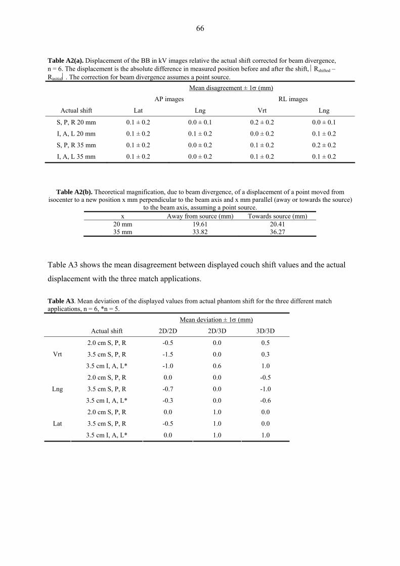
66

Table A2(a). Displacement of the BB in kV images relative the actual shift corrected for beam divergence, n = 6. The displacement is the absolute difference in measured position before and after the shift, ⎪Rshifted – Rinitial⎪. The correction for beam divergence assumes a point source.

Mean disagreement ± 1σ (mm)

AP images RL images

Actual shift Lat Lng Vrt Lng

S, P, R 20 mm 0.1 ± 0.2 0.0 ± 0.1 0.2 ± 0.2 0.0 ± 0.1

I, A, L 20 mm 0.1 ± 0.2 0.1 ± 0.2 0.0 ± 0.2 0.1 ± 0.2

S, P, R 35 mm 0.1 ± 0.2 0.0 ± 0.2 0.1 ± 0.2 0.2 ± 0.2

I, A, L 35 mm 0.1 ± 0.2 0.0 ± 0.2 0.1 ± 0.2 0.1 ± 0.2

Table A2(b). Theoretical magnification, due to beam divergence, of a displacement of a point moved from isocenter to a new position x mm perpendicular to the beam axis and x mm parallel (away or towards the source)

to the beam axis, assuming a point source. x Away from source (mm) Towards source (mm)

20 mm 19.61 20.41 35 mm 33.82 36.27

Table A3 shows the mean disagreement between displayed couch shift values and the actual

displacement with the three match applications.

Table A3. Mean deviation of the displayed values from actual phantom shift for the three different match applications, n = 6, *n = 5.

Mean deviation ± 1σ (mm)

Actual shift 2D/2D 2D/3D 3D/3D

2.0 cm S, P, R -0.5 0.0 0.5

3.5 cm S, P, R -1.5 0.0 0.3 Vrt

3.5 cm I, A, L* -1.0 0.6 1.0

2.0 cm S, P, R 0.0 0.0 -0.5

3.5 cm S, P, R -0.7 0.0 -1.0 Lng

3.5 cm I, A, L* -0.3 0.0 -0.6

2.0 cm S, P, R 0.0 1.0 0.0

3.5 cm S, P, R -0.5 1.0 0.0 Lat

3.5 cm I, A, L* 0.0 1.0 1.0