Evaluation of Different Turbulence Models and … · Evaluation of Different Turbulence Models and...

J. Energy Power Sources Vol. 1, Number 1, 2014, pp. 17-30 Received: July 2, 2014, Published: July 25, 2014

Journal of Energy and Power Sources

www.ethanpublishing.com

Evaluation of Different Turbulence Models and

Numerical Solvers for a Transonic Turbine Blade

Cascade

Amgad M. Abbass1, Medhat M. Sorour2 and Mohamed A. Teamah2

1. Maintenance Planning Sector, Abu Qir Fertilizers Co., El-Tabia Rashid road, Alexandria, Egypt

2. Mechanical Eng. Dept., Alexandria University, Alexandria, Egypt

Corresponding author: Amgad M. Abbas ([email protected])

Abstract: The gas path over the turbine blades is a very complex flow field due to the variation of flow regime and the corresponding heat transfer, This investigation is devoted to study the two and three-dimensional predictive modeling capability for airfoil external heat transfer by using pressure based solver PBS and density based solver DBS. The results show the effects of strong secondary vortexes, laminar-to-turbulent transition, and also show stagnation region characteristics. Simulations were performed on an irregular quadratic two and three-dimensional grids with the Fluent 6.3 software package employing several turbulence models (Spalart-Allmaras, RNG k-Є and SST k-ω model). Detailed heat transfer predictions are given for a power generation turbine rotor with

127° of nominal turning, axial chord of 130 mm and blade aspect ratio of 1.17. The comparison was made with the experimental and the

numerical results of Giel et al. and a good agreement was found with the DBS and Spalart-Allmaras turbulent model and it has been concluded in particular that rather fine computational three dimensional grids are needed to get accurate local heat transfer controlled by complex 3D structure of secondary flows. Key words: Transonic gas turbine, turbulent condition, pressure based solver PBS, density based solver DBS.

Nomenclature:

Cx Blade axial chord (m)

d Leading edge diameter (m)

h Heat transfer coefficient (W/m2-K)

K Thermal conductivity (W/m-K)

k Turbulent kinetic energy

M Mach number (dimensionless)

Nu Nusselt number (dimensionless)

P Pressure (Pa)

Pr Prandtl number (dimensionless)

Q Heat flux (W/m2)

Reex Reynolds number, Reex = ρUexCx

μ (dimensionless)

r Recovery factor, r=Pr1

3 S Blade surface length (m)

T Temperature (K)

Tu Turbulent Intensity (%)

U Free-stream velocity (m/s)

Y+ Dimensionless wall distance

Z Spanwise coordinate, normalized by blade span

Greek Symbols

γ Ratio of specific heats, (dimensionless)

Є Turbulent Dissipation Rate (m2/s3)

Λx Length scale (mm)

μ Dynamic viscosity (kg/s.m)

ρ Local Density (kg/m3)

ω Specific dissipation rate (s-1)

Subscripts

o Total condition

in Inlet free stream value

ex Exit free steam value

Isen Isentropic value

av Average value

aw Adiabatic wall value

1. Introduction

It is well known from the thermodynamic analysis

that the performance of a gas turbine engine is strongly

influenced by the temperature at the inlet to the turbine.

Evaluation of Different Turbulence Models and Numerical Solvers for a Transonic Turbine Blade Cascade

18

There is thus a growing tendency to use higher turbine

inlet temperatures, implying increasing heat loads to

the engine components. Modern gas turbine engines

are designed to operate at inlet temperatures of

1800-2000 K, which are far beyond the allowable

metal temperatures. Thus, to maintain acceptable life

and safety standards, the structural elements need to be

protected against the severe thermal environment. So

that as turbine inlet temperature increase, the necessity

for accurate heat transfer predictions also increases,

and for accurate heat transfer predictions.

With efficiency and power increases of modern gas

turbines, researchers tried continuously to increase the

inlet temperature to the maximum. This can be done

only with better blade cooling, great heat transfer

comprehension and three-dimensional distribution of

the temperature inside the turbine. To give a detailed

cooling analysis as well as a good thermal structure of

blades, several researchers treated experimentally and

numerically in this area as in the following

Experimental studies: Ref. [1] studied

experimentally the airfoil external heat transfer to

engine specific conditions including blade shape,

Reynolds numbers, and Mach numbers. Data were

obtained in steady-state using a thin-foil heater

wrapped around a low thermal conductivity blade with

127 deg of nominal turning and an axial chord of 130

mm. Surface temperatures were measured using

calibrated liquid crystals. The results showed the

effects of strong secondary vortical flows,

laminar-to-turbulent transition, and also show good

detail in the stagnation region.

Ref. [2] studied experimentally the local heat/mass

transfer characteristics on the stationary blade near-tip

surface for various relative positions of the blade. A

low speed wind tunnel with a stationary annular turbine

cascade was used. The test section has a single turbine

stage composed of sixteen guide plates and sixteen

blades. Detailed mass transfer measurements were

conducted for the stationary blade fixed at six different

relative blade positions in a single pitch using a

naphthalene sublimation method. They showed that

significantly different patterns are observed on the

blade surface, especially near the blade tip due to the

variation in tip leakage flow, and the heat/mass transfer

characteristics on the blade surface are affected

strongly by the local flow characteristics, such as

laminarization after flow acceleration, flow transition,

separation bubble and tip leakage flow.

Ref. [3] studied the Effect of rotation on detailed

film cooling effectiveness distributions in the leading

edge region of a gas turbine blade, with three

showerhead rows of radial-angle holes were the

effectiveness measured using the Pressure Sensitive

Paint (PSP) technique. Tests were conducted on the

first-stage rotor blade. The effect of the blowing ratio

was also studied. They showed that the different

rotation speeds significantly change the film cooling

traces with the average film cooling effectiveness in the

leading edge region increasing with blowing ratio.

Ref. [4] made a heat transfer analysis of gas turbine

blades using air or steam as coolants. Three main

schemes of the blade cooling were used, namely

air-cooling, Open-Circuit Steam Cooling (OCSC) and

Closed-Loop Steam Cooling (CLSC). The results

showed that steam appears to be a potential cooling

medium, when employed in an open-circuit or in a

closed-loop scheme. The combined system with CLSC

gives better overall performance than does air-cooling

or the OCSC.

Ref. [5] studied the effect of hole angle and hole

shaping in the turbine blade showerhead film cooling.

The film cooling measurements were presented on a

turbine blade leading edge model with three rows of

showerhead holes. They showed that, the shaping of

showerhead holes provides higher film effectiveness,

than just adding an additional compound angle in the

transverse direction and significantly higher

effectiveness than the baseline typical leading edge

geometry.

Numerical studies: Ref. [6] studied the Heat transfer

on a film-cooled rotating blade using a multi-block,


19

three-dimensional Navier-Stokes code to compute heat

transfer coefficient on the blade, hub and shroud for a

rotating high-pressure turbine blade with 172

film-cooling holes in eight rows. Wilcox’s k-ω model

was used for modeling the turbulence. Of the eight

rows of holes, three are staggered on the shower-head

with compound-angled holes. They showed that the

heat transfer coefficient is much higher on the blade tip

and shroud as compared to that on the hub for both the

cooled and the uncooled cases.

Ref. [7] performed a computation to predict the

three-dimensional flow and heat transfer of concave

plate that is cooled by two staggered rows of

film-cooling jets. This investigation considers two

coolant flow orientations. They showed that the

laterally averaged film-cooling effectiveness over the

concave surface with a straight-blow plenum is slightly

higher than that of a cross-blow plenum at all test

blowing ratios and the blowing ratio is one of the most

significant film-cooling parameters over a concave

surface.

Ref. [8] used the v2-f models of Durbin and the new

v2-f model of Jones et al. to compute the blade heat

transfer for the transonic cascade of Giel et al. Three

different experimental cases were considered. They

showed that the v2-f model of Durbin provides good

predictions on the pressure surface. But there is some

discrepancy between the suction surface heat transfer

predictions and experimental measurements. The

newer model of Jones et al. requires further

modification before it can be routinely used for blade

heat transfer.

Ref. [9] used two versions of the two-equation k-ω

model and a Shear Stress Transport (SST) model with a

three-dimensional, multi-block, Navier-Stokes code to

compare the detailed heat transfer measurements on a

transonic turbine blade. They showed that the SST

model resolves the passage vortex better on the suction

side of the blade, thus yielding a better comparison

with the experimental data than either of the k-ω

models. However, the comparison is still deficient on

the suction side of the blade. Use of the SST model

does require the computation of distance from a wall,

which for a multi-block grid, such as in This case, can

be complicated.

Ref. [10] studied numerically the transonic gas

turbine blade-to-blade compressible fluid flow, and

determined the pressure distribution around the blade

and compared the characteristic flow effects of

Reflecting Boundary Conditions (RBC) and

Non-Reflecting Boundary Conditions (NRBC) newly

implemented in FLUENT 6.0. They showed that the

modified k-Є, the Spalart-Allmaras and the RSM

models gives good results compared with experiment,

instead to use all these models to determine the effects

of reflecting and non-reflecting boundary conditions

only the RNG model is selected, also this model with

NRBCs formulation is used to see the effects of the

inlet turbulence intensities the exit Mach numbers and

the Inlet Reynolds numbers. The results are closest to

experiment.

The blade geometry used in the present study is

representative of first stage turbine blade for a new GE

heavy frame power turbine machine design and

presented in Fig.1.The turbine blade is for a machine

operating in the 1370 (2500) class. The full power

design point isentropic pressure ratio of the current

blade section is 1.443. The inlet Mach number is 0.399

and the exit isentropic Mach number is 0.743. The inlet

angle of attack is 59.1 deg while the exit angle is 67.9

deg, producing an aggressive total turning of 127 deg.

Fig. 1 Blade geometry.


20

The blades linear cascade was used in this study

because of the previous studies have shown that rotor

geometries in linear cascades provide good mid span

data as compared to their rotating equivalents.

The objective of the present study is to present the

results of predicted heat transfer of a transonic turbine

blade cascade obtained using ANSYS-FLUENT 6.3

CODE. One of the goals is to compare between the

solution which obtained using two different numerical

solvers such as Pressure Based Slover (PBS) and

density based solver (DBS) and study capability of a

three different turbulent models Spalart-Allmaras

model, RNG k-Є model and SST k-ω model.

2. Governing Equations

Reynolds-Averaged Navier-Stokes equations are the

governing equations for the problem analyzed

(momentum balance), with the continuity equation. For

the two and three-dimensional compressible flow of a

Newtonian fluid, mass and momentum equation

become, respectively

∂

∂xiρui = 0 (1)

∂

∂tρui +

∂

∂xjρuiuj = -

∂p

∂xi +

∂

∂xjμ

∂ui

∂xj+∂uj

∂xi-

2

3δij

∂ul

∂xl+

∂

∂xj-ρ ui

'uj' (2)

In Eq. (2), -ρ ui'uj

' is the additional term of

Reynolds stresses due to velocity fluctuations, which

has to be modeled for the closure of Eq. (2). The

classical approach is the use of Boussinesq hypothesis,

relating Reynolds stresses and mean flow strain,

through the eddy viscosity concept [11]. In its general

formulation as proposed by Kolmogorov, Boussinesq

hypothesis is written as:

-ρ ui'uj

' = μt∂ui

∂xj+∂uj

∂xi-

2

3ρk+μt

∂μk

∂xkδij (3)

Successful turbulence models are those based on the

eddy viscosity concept, which solve one and two and

seven scalar transport differential equations. The most

well-known is the k-ε model [12]. In turbulence models

that employ the Boussinesq approach, the central issue

is how the eddy viscosity is computed. The model [13]

solves a transport equation for a quantity that is a

modified form of the turbulent kinematic viscosity.

2.1 Spalart-Allmaras Model

The transported variable in the Spalart-Allmaras

model, v is identical to the turbulent kinematic

viscosity except in the near-wall (viscous-affected)

region. The transport equation for v:

∂

∂tρ v +

∂

∂xiρ vui = Cb1ρS v+

1

σv

∂

∂xjμ+ρ v

∂v

∂xj+Cb2 ρ

∂v

∂xj

2

-Cw1ρfwv

d

2 (4)

Note that since the turbulence kinetic energy k is not

calculated in the Spalart-Allmaras model, the last term

in Eq. (3) is ignored when estimating the Reynolds

stresses.

The eddy viscosity is given by

μt=ρvfv1 (5)

Where

fv1= X3

X3+ Cv13 6)

X≡ v

v (7)

fv2=1-X

1+X fv1 (8)

fw=g 1+Cw36

g6+Cw36

16 (9)

g=r+Cw2(r6-r) (10) ≡ v

Sκ2d2 (11)

S ≡S+ v

κ2d2 fv2 (12)

Where S is the magnitude of the vorticity and d is the

distance from the nearest wall. Acknowledged that one

should also take into account the effect of mean strain

on the turbulence production, and a modification to the

model has been proposed in Ref. [14] and incorporated


21

into the present study. This modification combines

measures of both rotation and strain tensors in the

definition of S:

S≡ Ωij + Cprod min 0, Sij - Ωij (13)

Ωij ≡ 2ΩijΩij, Sij ≡ 2SijSij (14)

The mean strain rate, Sij defined as:

Sij= 1

2

∂uj

∂xi-∂ui

∂xj (15)

The mean rate-of-rotation tensor, Ω defined as

Ωij= 1

2

∂ui

∂xj-∂uj

∂xi (16)

And the constants are Cb1=0.1355 , Cb2=0.622 ,

σv=2/3 , Cv1=7.1 , Cw1= Cb1

k2 +1+Cb2

σv, Cw2=0.3 ,

Cw3=2 , κ = 0.4187 and Cprod=2.0 which

represented in Ref. [14].

2.2 RNG k-Є Model

The RNG-based k-Є model is derived from the

instantaneous Navier-Stokes equations, using a

mathematical technique called “Renormalization

Group” (RNG) methods. The analytical derivation

results in a model with constants different from those in

the standard k-Є model, and additional terms and

functions in the transport equations for k and Є. A more

comprehensive description of RNG theory and its

application to turbulence can be found in Ref. [15].

The transport equations for the RNG k-Є model have

a similar form to the standard k-Є model:

∂

∂tρk +

∂

∂xiρkui =

∂

∂xjαkμeff

∂k

∂xj+Gk+Gb-ρϵ-YM (17)

And

∂

∂tρϵ +

∂

∂xiρϵui =

∂∂xj

αϵμeff∂ϵ

∂xj +C1ϵ

ϵ

kGk+C3ϵGb -C2ϵ

* ρϵ2

k (18)

The eddy viscosity is given by

μt=ρCμ k2

ϵ (19)

And after adding the swirl modification the eddy

viscosity becomes

μt=μt0f αs , Ω , K

ϵ (20)

Where μt0 is the value of turbulent viscosity

calculated without the swirl modification using Eq.

(19). Ω is a characteristic swirl number evaluated

within FLUENT, and αs is swirl constant and set to

0.07 for mildly swirling flow. This swirl modification

always takes effect for axisymmetric, swirling flows

and three-dimensional flows when the RNG model is

selected.

And C2ϵ* is given by:

C2ϵ* =C2ϵ+

Cμη3 1-η/η0

1+βη3 (21)

Where

η=S k

ϵ (22)

And the production of turbulence kinetic energy Gk

is given by:

Gk=μtS2 (23)

Where S is the modulus of the mean rate-of-strain

tensor, defined as:

S = 2SijSij (24)

Where Sij Calculated from Eq. (15)

The generation of k due to buoyancy in Eq. (17), and

the corresponding contribution to the production of Є

in Eq. (18).

Where Gb for ideal gases is given by:

Gb=-gi

μt

ρPrt

∂ρ

∂xi (25)

For the standard and realizable k-Є models, the

value of Prt is constant value of 0.85. In the case of the

RNG k-Є model, Prt=1

α, where α is given by:

α-1.3929

α0-1.3929

0.6321α+2.3929

α0+2.3929

0.3679 = μmol

μeff (26)

Where

α0= 1

Pr= k

μCp (27)


22

The Є is affected by the buoyancy is determined by

the constant C3Є. In FLUENT, C3Є is not specified, but

is instead calculated according to the following relation

which proposed in Ref. [16]:

C3ϵ= tanhv

u (28)

Where v is the component of the flow velocity

parallel to the gravitational vector and u is the

component of the flow velocity perpendicular to the

gravitational vector. And the effect of compressibility

according to a proposal Ref. [17] (YM) is given by:

YM=2ρϵMt2 (29)

Where Mt is the turbulent Mach number and defined

by:

Mt= k

a2 (30)

Where a is the speed of sound and given by:

a = γRT (31)

And the inverse effective Prandtl numbers, αkandαϵ,

are computed using Eq. (27) where α0 = 1 and in the

high-Reynolds-number limit (μmol

μeff≪1 ), ∝k=∝ϵ≈1.393.

The model constants are C1ϵ=1.42 , C2ϵ=1.68 ,

Cμ=0.0845, η0=4.38, β=0.012.

2.3 SST k-ω Model

The SST k-ω model [18] has a similar form to the

standard k-ω model [19] where the turbulence kinetic

energy, k, and the specific dissipation rate, ω are

obtained from the following transport equations:

∂

∂tρk +

∂

∂xiρkui = ∂∂xj

Γk∂k

∂xj+Gk-Yk+Sk (32)

And

∂

∂tρω +

∂

∂xiρωui =

∂

∂xjΓω

∂ω

∂xj+Gω-Yω+Dω+Sω (33)

Where the effective diffusivities for the k-ω model

are given by:

Γk=μ+μt

σk (34)

Γω=μ+μt

σω (35)

Where Sis the strain rate magnitude and the turbulent

Prandtl numbers for k and ω is given by

σk= 1

F1σk,1

+1-F1σk,2

(36)

σω= 1

F1σω,1

+ 1-F1σω,2

(37)

Where F1 and F2 are given by:

F1= tanh Φ14 (38)

Φ1=min max√k

0.09 ω y,

500 μ

ρy2ω,

4ρk

σω,2Dω+ y2 (39)

Dω+ =max 2ρ

1

σω,2

1

ω

∂k

∂xj

∂ω

∂xj, 10-10 (40)

Where μt is the turbulent eddy viscosity and given

by:

μt= ρkω 1

max1

α*, SF2a1ω

(41)

Where the coefficient ∗ damps the turbulent

viscosity causing a low-Reynolds-number correction

and given by:

α*=α∞* α0*+ Ret/Rk

1+Ret/Rk (42)

Where

Ret= ρkμω (43)

α0 * =

βi

3 (44)

βi=0.072 (45)

And is given by:

F2= tanh Φ22 (46)

Φ2=max 2√k

0.09 ω y ,

500 μ

ρy2ω (47)

Where, y is the distance to the next surface.

The production of k ( ) is given by:

Gk= min Gk, 10ρβ*kω (48)

Where

Gk= μtS2 (49)


23

β*=βi* 1+ζ*F(Mt) (50)

βi*=β∞* 4

15+

RetRβ

4

1+ RetRβ

4 (51)

And the compressibility function F(Mt) is given by:

F(Mt) = 0 Mt≤Mt0

Mt2-Mt0

2 Mt>Mt0 (52)

Where

Mt2=

2k

a2 (53)

Where (a) is the sonic speed calculated from Eq. (31)

and the production of ω (Gω) is given by:

Gω=α ωk Gk (54)

Where ∝= ∝∞∝*

∝0+Ret/RW

1+Ret/RW (55)

Where ∝∞ is given by:

α∞=F1α∞,1+ 1-F1 α∞,2 (56)

Where

α∞,1= βi,1

β∞* -

κ2

σω,1 β∞

*

, α∞,2= βi,2

β∞* -

κ2

σω,2 β∞

*

(57)

The Dissipation of k (Yk) is given by:

Yk= ρβ*kω (58)

The Dissipation of ω (Yω) is given by:

Yω= ρβω2 (59)

Where β=βi 1-βi

*

βiζ*F Mt (60)

Instead of a having a constant value, βi is given by:

βi=F1βi,1+ 1-F1 βi,2 (61)

And the constants are σk,1=1.176, σω,1=2, σk,2=1,

σω,2=1.168 , a1=0.31 , βi,1=0.075 , βi,2=0.0828 ,

α∞* =1, α0=1/9, β∞

* =0.09, Rβ=8, Rk=6, Rω=2.95,

κ = 0.41, ζ*=1.5, Mt0=0.25.

3. Convective Heat Transfer

In FLUENT, turbulent heat transport is modeled

using the concept of Reynolds’ analogy to turbulent

momentum transfer. The “modeled” energy equation is

thus given by the following:

∂

∂tρCPT +

∂

∂xiρui CPT+1 =

∂

∂xjKeff

∂T

∂xj+ui τij eff

(62)

Where τij eff is the deviatoric stress tensor and

given by:

τij eff=μeff

∂uj

∂xi+∂ui

∂xj-

2

3μeff

∂uk

∂xkδij (63)

For Spalart-Allmaras and SST-kω models, the

effective thermal conductivity is given by:

Keff=K+Cpμt

Prt (64)

Where, a constant value of 0.85 is used for the

turbulent Prandtl number. But for the RNG, the

effective thermal conductivity is given by:

Keff=∝Cpμeff (65)

4. Numerical Methods

The study domain consists of one passage with an

inlet zone located at 15.24 cm from the leading edge; it

is limited by the blades pitch length 13 cm. The blade

profiles were obtained by creating real edges from a

given 143 points defining the blade geometry.

GAMBIT forms the edges in the shape of general

NURBS curve of degree n which is GAMBIT employs

a value of n = 3 Fig. 1 (NURBS is a specific notation to

Gambit it is describes how to create real curve from

existing points).

The irregular quadratic semi structured grid is

generated by the pre-processor GAMBIT (v2.3.16).

According to this complex geometry, the grid is

obtained using the QUAD PAVE scheme for the 2-d

mesh which used in the 2D case as shown in Fig. 2

and with total number of cells as shown in Table 1 ,

the grid which used in the 3d case is obtained using

the 2D grid as the base of the 3D grid volume , the 3D


24

grid was generated using the HEX-WEDGE COOPER

scheme with 30 cells in span wise direction as shown

in Fig. 3, the total number of cells are as shown in

Table 1. Near-wall grid is ‘‘adapted” using the

boundary layer method as to capture the important

characteristics of the turbulent flow and to make the

grid independence. Adaptation refines the grid in both

streamwise and spanwise directions. The refined grid

along the wall region reduces the first y+ to lower than

value of 5. The grid independent study was conducted

to achieve a very small change in average Nusselt

number on turbine blade suction and pressure side.

The commercial software package FLUENT (V. 6.3)

from ANSYS, Inc. is adopted in this study. Fluent

employs a finite-volume method with second order

upwind scheme for spatial discretization of the convective

Fig. 2 The computational grid of two dimensional models.

Table 1 Grid size parameters values.

Cells Faces Nodes

2D Mesh 7687 15526 7934

3D Mesh 215236 657651 230086

Fig. 3 The computational grid of three dimensional models.

terms. The initial values were taken from the inlet

boundary condition.

We made use of “Coupled solution method” [20].

Using this approach, the governing equations are

solved simultaneously, i.e., coupled together.

Governing equations for additional scalars will be

solved sequentially. A control volume-based technique

is used that consists of:

• Division of the domain into discrete control

volumes using a computational grid;

• Integration of the governing equations on the

individual control volumes to construct algebraic

equations for the discrete dependent variables

(unknowns) such as velocities, pressure, temperature,

and conserved scalars;

• Linearization of the discretized equations and

solution of the resultant linear equation system to yield

updated values of the dependent variables. The coupled

approach is designed for high speed compressible

flows and gives very satisfactory results in turbo

machines especially with the implicit coupled solver.

The second order upstream [20] scheme is used

because higher-order accuracy is desired.

5. Boundary Conditions

The boundary conditions are very important to

obtain an exact solution with a rapid convergence.

According to the theory of characteristics, flow angle,

total pressure, total temperature, and isentropic

relations are used at the subsonic inlet. The same

relations are used to determine the fluid properties at

the supersonic outlet such as static pressure, static

temperature and the isentropic exit Mach number. All

of the fluid properties which used as a boundary

condition for the present study cases are described

below and in Table 2:

• All the walls (pressure and suction sides) are

considered Isothermal 345oK with no slip condition,

the temperature of the unheated endwall was set equal

to the inlet total temperature and mid span symmetry

was assumed;


25

Table 2 Boundary conditions of the present cases.

Reex (%) Reex Min Po in Pin Pex

100 2488000 0.352 156790.9 143896.4 108776.8

75 1866000 0.352 117593.2 107922.3 81582.57

50 1244000 0.352 78395.4 71948.19 54388.38

30 746400 0.352 47037.2 43168.92 32633.03

• Since the periodic boundaries are satisfied,

instead of modeling the whole blades row of 11

passages of Ref. [1], only one passage is used in order

to limit the computational time and costs;

• Total pressure, total temperature 300oK, inlet total

and static pressure, inlet flow angle and inlet Tu = 9%

and ΛX = 0.026 m, are specified as the inlet conditions;

• Outlet static pressure according to Mex = 0.742 and

outlet flow angle is specified as the outlet conditions.

6. Nusselt Number

The Nusselt number was defined as follows:

Nu= h.Cx

K(To in) (66)

Where is the heat transfer coefficient h is defined as:

h= Qw

(Tw-Taw) (67)

Where the local adiabatic wall temperature Taw is

defined as:

Taw= r+ 1-r1+0.5 γ-1 Misen

2 *To in (68)

In expression (3) the local isentropic Mach number

Misen, is determined from the wall static pressure, and

the recovery factor r is evaluated as:

r=Pr13 (69)

Pr= μ Cp

K(To in) (70)

7. Results and Discussion

Figs. 4-7 show isentropic Mach number distribution

over the blade mid span for the 2D and 3D models

computed with three turbulence models and with two

different numerical solvers (Pressure based solver PBS

and Density based solver DBS ) in comparison with the

measured and another numerical data. These

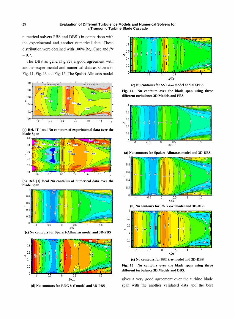
distribution were obtained with 100% Reex Case and Pr

= 0.7. generally can concluded that all models capture

the main trends and no significant difference between

the turbulence models and the numerical solvers which

used but the 3D models gives more accurate results

near the suction side trailing edge as shown in Figs 6-7.

Figs. 8-9 show isentropic Mach number contours

over the blade span for the 3D model computed with

three different turbulence models using the PBS and

DBS in comparison with another numerical data. These

Fig. 4 Comparison of Misen over the blade mid span using three different turbulence 2D models and PBS.

Fig. 5 Comparison of Misen over the blade mid span using three different turbulence 2D models and DBS.

-1.0 -0.5 0.0 0.5 1.0 1.5 2.00.0

0.2

0.4

0.6

0.8

1.0

Mis

en

S/Cx

2d -PBS. RNG k-ε 2d -PBS. Sst k-ω 2d -PBS. Spalart-A. G iel [11] :Calc. G iel [11] :Expr.

-1.0 -0.5 0.0 0.5 1.0 1.5 2.00.0

0.2

0.4

0.6

0.8

1.0

Mis

en

S /Cx

G ie l [11] : Ca lc G iel [11] : Exp. 2d- DBS SSTk−ω 2d- DBS R NG k−ε 2d- DBS Spalart-A .

26

Fig. 6 Compathree different

Fig. 7 Compathree different

(a) Ref. [1] Mi

span

(b) 3D-PBS M

-1.00.0

0.2

0.4

0.6

0.8

1.0

Mis

en

-1.00.0

0.2

0.4

0.6

0.8

1.0

1.2

Mis

enEval

arison of Misen t turbulence 3D

arison of Misen t turbulence 3D

isen contours of

Misen contours u

-0.5 0.0

-0.5 0.0

luation of Diffa

over the bladeD models and PB

over the bladeD models and D

f numerical dat

using Spalart-A

0.5 1.0

S/Cx

3d 3d 3d Gie Gie

0.5 1.0

S/Cx

G G 3d 3d 3d

ferent Turbulea Transonic T

e mid span usinBS.

e mid span usinBS.

ta over the blad

Allmaras model

0 1.5 2

- PBS. RNG k-ε- PBS. Sst k-ω- PBS. Spalart-A.

el [11] :Calc.el [11] :Expr.

1.5 2.0

Giel [11] : Calc Giel [11] : Exp.d-DBS. SSTk−ωd-DBS. RNGk−εd-DBS. Spalart-A.

ence Models aurbine Blade

ng

ng

de

l

(c

(d

Fig. 8differen

contou

All tur

agreem

the RN

excepti

From

numbe

are see

throat

occur

Decele

downst

-0.35.

heat tra

Figs

the bla

with th

numeri

the m

distribu

= 0.7.

.0

0

and NumericaCascade

c) 3D-PBS Misen

d) 3D-PBS Mise

Misen contount turbulence 3

urs obtained w

rbulence mod

ment with the

NG k-Є mo

ions in data ov

m all figures w

er concluded

en on the sucti

at S/Cx = 1.

on the un

eration also s

tream of the l

The calculate

ansfer parame

s. 10-13 show

de mid span fo

hree turbulenc

ical solvers P

measured and

ution were ob

al Solvers for

n contours using

en contours usin

rs over the bD models and P

with 100 % Re

dels and solv

another num

odel with th

ver the suctio

which present

that no decel

ion surface un

07 where ver

covered por

seen on the p

leading edge,

ed values Mis

eters calculatio

local Nu num

for the 2D and

ce models an

BS and DBS

another num

btained with 10

g RNG K-Є mo

ng SST k-ω mod

blade span usiPBS.

eex Case and P

vers gives ver

merical results

he PBS give

n side.

s the isentrop

lerating flow

ntil near the ge

ry slight dece

rtion of the

pressure surf

extending to

sen were used

on.

mber distributi

3D models co

nd with two d

) in comparis

merical data

00% Reex case

odel

del

ng three

Pr = 0.7.

ry good

s except

es some

ic Mach

regions

eometric

eleration

blade.

face just

o S/Cx =

d for the

ion over

omputed

different

son with

. These

e and Pr

(a) 3D-DBS

(b) 3D-D

(c) 3D-D

Fig. 9 Misen different turbu

Fig. 10 Comspan using thre

-1.0

2000

4000

6000

Nu

Eval

Misen contours

DBS Misen conto

DBS Misen cont

contours overulence 3D mode

parison of theee different tur

-0.5 0.0S/

luation of Diffa

for Spalart-Al

ours for RNG k

ours for SST k-r the blade spels and DBS.

e local Nu overrbulence 2D mo

0.5 1.0/Cx

Gi Gi 2d 2d 2d


llmaras model

k-Є model

-ω model

pan using thre

r the blade miodels and PBS.

1.5 2.

el [11] : Exp.el [11] : Calc.

d PBS. Spalart A.d PBS. RNG k-εd PBS. SST k-ω


ee

id

Fig. 11span us

Fig. 12 span us

Fig. 13 span us

Figs

blade s

three

.0

1000

1500

2000

2500

3000

3500

4000

4500

5000

5500

6000

6500

Nu

2000

4000

6000

Nu

500

1000

1500

2000

2500

3000

3500

4000

4500

5000

5500

6000

6500

7000

Nu

and NumericaCascade

Comparisonsing three differ



s. 14-15 show

span for the 2

turbulence m

-1.0 -0.5

-1.0 -0.5

-1 .0 -0 .5

al Solvers for

n of the local Nrent turbulence



local Nu num

2D and 3D m

models and

0.0 0.5S/Cx

0.0 0.5

S/Cx

0 .0 0.5

S/C x

Nu over the ble 2D models an



mber contours

models comput

with two d

1.0 1.5

Giel [11] : E Giel [11] : C 2d-DBS Sp 2d-DBS RN 2d-DBS SS

1.0 1.5

Giel [11] : Giel [11] : 3d-PBS. S 3d-PBS. R 3d-PBS. S

1.0 1 .5

G ie l [11 ] : E x G ie l [11 ] : C a 3d -D B S . S pa 3d -D B S . R N 3d -D B S . S S T

27

lade mid

nd DBS.

lade mid nd PBS.

lade mid

nd DBS.

over the

ted with

different

5 2.0

xp.alcalart-A.

NGk−εSTk−ω

5 2.0

Exp.Calc.

Spalart A.RNG k-εSST k-ω

5 2.0

xp .a lc .a la rt-A .G k −εTk −ω

28

numerical sol

the experime

distribution w

= 0.7.

The DBS

another exper

Fig. 11, Fig. 1

(a) Ref. [1] locblade Span

(b) Ref. [1] loblade Span

(c) Nu contou

(d) Nu co

Eval

lvers PBS and

ental and ano

were obtained

as general gi

rimental and

13 and Fig. 15.

cal Nu contours

ocal Nu contou

urs for Spalart-

ontours for RNG

luation of Diffa

d DBS ) in co

other numeric

with 100% Re

ives a good a

numerical da

The Spalart-A

s of experiment

urs of numerica

-Allmaras mod

G k-Є model an


omparison wit

cal data. Thes

eex Case and P

agreement wit

ata as shown i

Allmaras mode

tal data over th

al data over th

del and 3D-PBS

nd 3D-PBS


th

se

Pr

th

in

el

he

he

S

(e

Fig. 14differen

(a) Nu

(b

(c

Fig. 15differen

gives a

span w

and NumericaCascade

e) Nu contours

4 Nu contournt turbulence 3

u contours for S

b) Nu contours

c) Nu contours

5 Nu contournt turbulence 3

a very good

with the anot

al Solvers for

for SST k-ω m

rs over the bD Models and P

Spalart-Allmar

for RNG k-Є m

for SST k-ω m

rs over the bD Models and D

agreement ov

ther validated

model and 3D-PB

lade span usinPBS.

ras model and 3

model and 3D-D

model and 3D-D

lade span usinDBS.

ver the turbin

d data and t

BS

ng three

3D-DBS

DBS

BS

ng three

ne blade

the best


29

agreement shown over the leading edge and the suction

side as shown in Fig. 11, Fig. 13 and Fig. 15. The other

turbulence models with the DBS give a good

agreement over the turbine blade span and the best

agreement with RNG k-Є and SST k-ω models shown

on the pressure and suction sides and bad agreement

near the leading edge due to transition relaminarization

effect which occur near the leading edge.

Tables 3-4 present the average Nu over the blade

mid span and whole span percentage of uncertainty

comparison between every turbulence model used in the

Table 3 Average Nu % of deviation over the turbine blade mid span for 2D cases.

Spalart-Allmaras RNG k-Є SST k-ω 2D PBS 4.7 27.54 7.638

2D DBS 4.39 9.56 4.42

Table 4 Average Nu % of deviation over the turbine blade span for 3D cases.

Spalart-Allmaras RNG k-Є SST k-ω 3D PBS 5.49 28.38 6.95

3D DBS 4.2 13.76 4.7

(a) Pressure Side and leading edge

(b) Suction side

Fig. 16 Stream lines around the half span turbine blade cascade.

present study with PBS and DBS for the 2D and 3D

models.

From Tables 3-4 concluded that generally the DBP

gives more accurate results than the PBS for each

turbulence model and for any shape of grid (2D and

3D models) and the Spalart-Allmaras turbulent model

gives more accurate average Nu over the blade span

than the other turbulent models for the 3D model so

the Spalart-Allmaras model chosen to predict the heat

transfer over a turbine blade for a different loads.

The horse shoe vortex shown over the suction sides

near the unheated end wall (T = To in) and covers the

suction side from the geometric throat to the trailing

edge along the uncovered portion of the suction side as

shown in Fig. 16(b). No vortex shown over the whole

pressure side as shown in Fig. 16(a).

8. Conclusions

• Splart-Allmaras model with the DBS gives the

best agreement of the calculated Nu with previous

experimental results for both 2D and 3D models. In

addition DBS gives more accurate results than the PBS

for all turbulence models which was used in the present

study;

• No vortex appeared over the pressure side but a

horse shoe vortex appeared on the suction side;

• Three peaks of Nu appeared in the present

investigation, the known peak near the stagnation and

other two peaks near the end walls. This conclusion

indicate the need to use 3D models for studding the

heat transfer over the turbine blade due to the complex

structure of secondary flows.

References

[1] P.W. Giel , R.J. Boyle, R.S. Bunker , Measurements and predictions of heat transfer on rotor blades in a transonic turbine cascade, ASME J. of Turbomachinery 126 (1) (2004) 110-121.

[2] H.H. Cho, D.H. Rhee, Effect of vane/blade relative position on heat transfer characteristics in a stationary turbine blade: Part 2. Blade surface, International Journal of Thermal Sciences 47 (11) (2008) 1544-1554.

[3] J.C. Han, J.Y Ahn, M.T. Schobeiri, H.K. Moon, Effect of


30

rotation on leading edge region film cooling of a gas turbine blade with three rows of film cooling holes, International Journal of Heat and Mass Transfer 50 (2007) 15-25.

[4] M.H. Albeirutty, A.S. Alghamdi, Y.S. Najjar , Heat transfer analysis for a multistage gas turbine using different blade-cooling schemes, Applied Thermal Engineering 24 (4) (2004) 563-577.

[5] S.V. Ekkad, Y.P. Lu, D. Allison, Turbine blade showerhead film cooling: Influence of hole angle and shaping, International Journal of Heat and Fluid Flow 28 (5) (2007) 922-931.

[6] V.K. Garg, Heat transfer on a film-cooled rotating blade, International Journal of Heat and Fluid Flow 21 (2) (2000) 134-145.

[7] J.M. Miao, H.K. Ching, Numerical simulation of film-cooling concave plate as coolant jet passes through two rows of holes with various orientations of coolant flow, International Journal of Heat and Mass Transfer 49 (2006) 557-574.

[8] A.A. Ameri, K. Ajmani, Evaluation of predicted heat transfer on a transonic blade using ν 2-ƒ models, ASME Turbo Expo 2004: Power for Land, Sea, and Air, June 2004.

[9] V.K. Garg, A.A. Ameri, Two-equation turbulence models for prediction of heat transfer on a transonic turbine blade, International Journal of Heat and Fluid Flow 22 (6) (2001) 593-602.

[10] P.W. Giel, S. Djouimaa, L. Messaoudi, Transonic turbine blade loading calculations using different turbulence models-effects of reflecting and non-reflecting boundary

conditions, Applied Thermal Engineering 27 (4) (2007) 779-787.

[11] J.O. Hinze, Turbulence, McGraw-Hill Publishing Co., New York, 1975.

[12] B.E. Launder, D.B. Spalding, 1974. “The Numerical computation of Turbulent Flows”, Computer Methods in Applied Mechanics and Engineering 3 (1974) 269-289.

[13] P. Spalart, S. Allmaras, A One-Equation Turbulence Model for Aerodynamic Flows, Technical Report AIAA-92-0439, American Institute of Aeronautics and Astronautics, 1992.

[14] J.D. Mariani, G.G. Zilliac, J.S. Chow, P. Bradshaw, Numerical/Experimental study of a wing tip vortex in the near field, AIAA Journal 33 (9) (1995) 1561-1568.

[15] D. Choudhury, Introduction to the renormalization group method and turbulence modeling, Fluent Inc. Technical Memorandum TM-107, 1993.

[16] R.A.W.M. Henkes, F.F. van der Flugt, C.J. Hoogendoorn, Natural convection flow in a square cavity calculated with low-reynolds-number turbulence models, Int. J. Heat Mass Transfer 34 (1991) 1543-1557.

[17] S. Sarka, L. Balakrishnan, Application of a Reynolds-Stress Turbulence Model to the Compressible Shear Layer, ICASE Report 90-18, NASA CR 182002, 1990.

[18] F.R. Menter, Two-Equation eddy-viscosity turbulence models for engineering applications, AIAA Journal 32 (8) (1994) 1598-1605.

[19] D.C. Wilcox, Turbulence modeling for CFD, DCW Industries Inc., La Canada, California, 1998.

[20] Fluent 6.3 User Guide, Fluent Inc., 2006.

Evaluation of Different Turbulence Models and … · Evaluation of Different Turbulence Models and...

Documents

Transcript of Evaluation of Different Turbulence Models and … · Evaluation of Different Turbulence Models and...