Evaluation of Different Concepts for Pressed and Sintered ...
69
Evaluation of Different Concepts for Pressed and Sintered Connecting Rods Mattias Rehn Mechanical Engineering, master's level 2019 Luleå University of Technology Department of Engineering Sciences and Mathematics
Transcript of Evaluation of Different Concepts for Pressed and Sintered ...
Evaluation of Different Concepts for
Pressed and Sintered Connecting Rods
Mattias Rehn
Mechanical Engineering, master's level
2019
Luleå University of Technology
Department of Engineering Sciences and Mathematics
Abstract
Connecting rod are found in most combustion engines and transmits thrust from the
piston to the crankshaft. The connecting rod needs to withstand forces from the piston
and inertia forces which results in axial tension, compression stresses and bending.
Today the most common manufacturing techniques in automotive industry are drop-
forging, die-casting and the Powder Metallurgy technique used is powder-forging.
In this Master Thesis different connecting rod designs for a single press PM manufac-
turing process were created and evaluated as a part of Hoganas AB’s Total Powder
Metal Car project, TPMC. This paper will serve as a basis for future connecting rod
projects at Hoganas AB when choosing a suitable connecting rod design.
The main objective of this Master Thesis is to evaluate different designs in regards to
the following:
• Buckling strength
• Fatigue life
• Manufacturing rating
The study shows that there is evidence that a single pressed connecting rod is possible.
No absolute answer of which design is the best is given in this paper since in depends
on different parameters and application. For each parameter examined there are results
presented and arguments for and against each design which can aid designers in future
work.
Suggestions of improvement on both the method and on the designs are presented in
respect to the results. The improvements may potentially increase the fatigue life,
buckling strength and improve manufacturability.
i

Preface
This master thesis were made at Hoganas AB in the beginning of 2019 and I would like
to thank them for giving me the opportunity to make my master thesis there.
I would like to first thank my supervisor at Hoganas AB, Michael Andersson for all the
help, support and guidance throughout the project. Also a special thanks to Thomas
Schmidtseifer for all the help and counseling regarding the manufacturing part of this
thesis.
Further I would like to thank my examiner Jesper Sundqvist from Lulea University of
Technology for all the help.
Many thanks to all the other master thesis students at Hoganas AB for their help and
all the laughters during this thesis.
ii

Contents
1 Introduction 3
1.1 Objective . . . . . . . . . . . . . . . . . . . . . . . . . . . . . . . . . . 4
1.2 Delimitations . . . . . . . . . . . . . . . . . . . . . . . . . . . . . . . . 4
2 Theory 5
2.1 Product Development Process . . . . . . . . . . . . . . . . . . . . . . . 5
2.1.1 Concept Generation . . . . . . . . . . . . . . . . . . . . . . . . 5
2.1.2 Screening and Scoring . . . . . . . . . . . . . . . . . . . . . . . 5
2.2 Powder Metallurgy, PM . . . . . . . . . . . . . . . . . . . . . . . . . . 6
2.3 Connecting Rod . . . . . . . . . . . . . . . . . . . . . . . . . . . . . . . 10
2.3.1 Forces . . . . . . . . . . . . . . . . . . . . . . . . . . . . . . . . 11
2.3.2 Buckling . . . . . . . . . . . . . . . . . . . . . . . . . . . . . . . 14
2.3.3 Fatigue . . . . . . . . . . . . . . . . . . . . . . . . . . . . . . . . 14
2.3.4 Material . . . . . . . . . . . . . . . . . . . . . . . . . . . . . . . 18
2.4 Finite Element Analysis . . . . . . . . . . . . . . . . . . . . . . . . . . 21
3 Methodology 22
3.1 Concept generation . . . . . . . . . . . . . . . . . . . . . . . . . . . . . 22
3.2 Modeling . . . . . . . . . . . . . . . . . . . . . . . . . . . . . . . . . . . 22
3.3 Finite Element Analysis . . . . . . . . . . . . . . . . . . . . . . . . . . 23
3.4 Manufacturing ranking . . . . . . . . . . . . . . . . . . . . . . . . . . . 25
4 Results 26
4.1 Concepts . . . . . . . . . . . . . . . . . . . . . . . . . . . . . . . . . . . 26
4.2 Fatigue . . . . . . . . . . . . . . . . . . . . . . . . . . . . . . . . . . . . 29
4.3 Buckling . . . . . . . . . . . . . . . . . . . . . . . . . . . . . . . . . . . 30
4.4 Manufacturing ranking . . . . . . . . . . . . . . . . . . . . . . . . . . . 32
5 Discussion 33
5.1 Buckling . . . . . . . . . . . . . . . . . . . . . . . . . . . . . . . . . . . 33
5.2 Fatigue . . . . . . . . . . . . . . . . . . . . . . . . . . . . . . . . . . . . 33
5.2.1 Concept 1 . . . . . . . . . . . . . . . . . . . . . . . . . . . . . . 34
5.2.2 Concept 2 . . . . . . . . . . . . . . . . . . . . . . . . . . . . . . 34
iii

5.2.3 Concept 4 . . . . . . . . . . . . . . . . . . . . . . . . . . . . . . 35
5.2.4 Concept 5 . . . . . . . . . . . . . . . . . . . . . . . . . . . . . . 35
5.2.5 Concept 7 . . . . . . . . . . . . . . . . . . . . . . . . . . . . . . 36
5.2.6 Concept 14 . . . . . . . . . . . . . . . . . . . . . . . . . . . . . 36
5.3 Finite Element Analysis . . . . . . . . . . . . . . . . . . . . . . . . . . 36
5.4 Manufacturing ranking . . . . . . . . . . . . . . . . . . . . . . . . . . . 37
5.4.1 Concept 1 . . . . . . . . . . . . . . . . . . . . . . . . . . . . . . 37
5.4.2 Concept 2 . . . . . . . . . . . . . . . . . . . . . . . . . . . . . . 37
5.4.3 Concept 4 . . . . . . . . . . . . . . . . . . . . . . . . . . . . . . 37
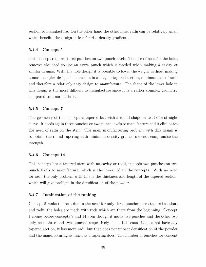
5.4.4 Concept 5 . . . . . . . . . . . . . . . . . . . . . . . . . . . . . . 38
5.4.5 Concept 7 . . . . . . . . . . . . . . . . . . . . . . . . . . . . . . 38
5.4.6 Concept 14 . . . . . . . . . . . . . . . . . . . . . . . . . . . . . 38
5.4.7 Justification of the ranking . . . . . . . . . . . . . . . . . . . . . 38
6 Conclusions 40
7 Future work 41
A Derivation 43
B Data for FEA 46
C Stress data from FEA 47
D Concepts 55
E Critical points in Haigh-diagram 58
iv

Nomenclature
Ap Area of piston [m2]
a Connecting rod length, c-c small and big eye [m]
ax Acceleration on the connecting rod in x-direction [m/s2]
ay Acceleration on the connecting rod in y-direction [m/s2]
b Distance from center of gravity to pin end [m]
c Distance from center of gravity to crank end [m]
Fp Piston force [N ]
Fx Force in x-direction on the pin end [N ]
Fy Force in y-direction on the pin end [N ]
I Moment of inertia on connecting rod [kg ·m2]
mc Mass of connecting rod [kg]
mp Mass of piston [kg]
n Safety factor [−]
P Pressure on piston [Pa]
R Stress ratio [−]
r Crank length [m]
Tx Force in x-direction on the crank end [N ]
Ty Force in y-direction on the crank end [N ]
xg Distance to center of gravity in x-direction [m]
1

xg Velocity of center of gravity in x-direction [m/s]
y Distance from origin to pin end [m]
y Velocity in y-direction [m]
y Acceleration in y-direction [m/s2]
yg Distance to center of gravity in y-direction [m]
yg Velocity of center of gravity in y-direction [m/s]
ω Angular velocity around crank end [rad/s]
σa Alternating stress [MPa]
σm Mean stress [MPa]
σmax Maximum stress [MPa]
σmin Minimum stress [MPa]
θ Crank angle [−]
ϕ Angle between connecting rod centerline and piston centerline [−]
ϕ Angular velocity around pin end [rad/s]
ϕ Angular acceleration around pin end [rad/s2]
2
1 Introduction
This Master Thesis is an evaluation study on the design of connecting rods for Powder
Metallurgy (PM) manufacturing and it was done at Hoganas AB as a part of their Total
Powder Metal Car project, TPMC. This study will serve as a basis in future projects at
Hoganas AB when choosing which design that will be best suitable for a specific case.
Connecting rods are used in most combustion engines to transmit the thrust from the
piston to the crankshaft. The connecting rods are subjected to cyclic loading and needs
to be strong enough to not break during the cycles, but also be light to minimize the
inertia forces. The loads vary from compressive loads due to the combustion and tensile
loads due to inertia.
The most common production techniques for connecting rods are drop-, powder-forging
and die-casting. For manufacturing high volumes of connecting rods, forged steel were
the best way of producing them for a long time, but since the powder metal processes
were introduced, these two techniques are the most competitive manufacturing pro-
cesses. This because of the cost efficiency of PM connecting rods resulting in almost
net shape which reduces the used material with equal strength and quality.[1]
The technique used today for manufacturing PM connecting rods for the automotive
industry are powder forging and it is made by pressing, sintering, reheating and forging
to obtain full density[2]. The technique is well established but to lower the production
time and cost Hoganas AB wants to manufacture a connecting rod through the standard
PM process with single compaction and sintering combined with sinter hardening and
obtain similar performance.
3

1.1 Objective
The objective of this thesis is to create a basis for future connecting rod projects by
creating five or more concepts of different design using an existing connecting rod from
a VW 1.4 TSI four-cylinder-in-line engine as a reference. The different concepts will
be evaluated using Finite Element Analysis and then benchmarked against each other
and the original to determine which design is best from a strength and manufacturing
perspective. The scope is to focus at the transition from the small and big eye to the
stem and also at the stem. The different parameters for comparison are:
• Buckling strength
• Fatigue life
• Manufacturing rating
1.2 Delimitations
Since a specific connecting rod is chosen as a reference, there are limitations in the
overall size of the concepts to fit in the existing engine. The weight and its distribution
is also important so the weight must be±10g of the original and the center of gravitation
should remain as close as possible to the original.
4

2 Theory
This section explains the product development process, powder metallurgy process, the
different challenges when designing a connecting rod and how to solve them.
2.1 Product Development Process
Ulrich and Eppinger’s [3] product development process was used in this paper to struc-
ture the development of the designs. Since this study will not lead to a finished product
only the concept generation, screening and scoring parts of the process were used.
2.1.1 Concept Generation
The concept generation process starts with a problem formulation and the target speci-
fication. It ends up with a number of concepts to solve the initial problem. Even though
the concept generation is a creative process there is need for a structured method to
explore all of the design room and not miss a solution. The process can be divided in
to the following steps:
• Clarify the problem
• Search information externally and internally
• Work systematically
• Reflect in the results
2.1.2 Screening and Scoring
The concept selection process is used to evaluate the concept with the respect to the
given specification. The concepts are compared in regards of relative strengths and
weaknesses to be able to select the concepts to further develop. Both the screening and
scoring is done with a selection matrix.
The screening uses a reference concept to evaluate the other ones against with the use
of selection criteria while the scoring can uses different reference points. The screening
is a rough comparison method while the scoring uses a finer rating scale with weighted
5
criteria. After each of the processes there is often a possibility to combine and improve-
ment the concepts, sometimes new concept is created and the process starts again.
These iterative processes are a good way to improve and find the optimal concept.[3]
2.2 Powder Metallurgy, PM
The densifying starts with the metal powder being filled in a die cavity by gravity
and compacted under high pressure from top and bottom at the same time achieving
relative homogeneous density as seen in Figure 2.1. The particles are compacted so
close that their irregularities interlock and cold welding occurs between them.
Figure 2.1: Basic press cycle with three stages: filling, densifying and ejection. [4]
There are several parameters to have in mind when designing the compaction tool e.g.
every portion of the cavity must be filled the right amount of powder, the tool should
have as few punches as possible and the densification should happen at the same time
in all of the cavity. The powder flows very little sideways during densification which
has to be considered to achieve homogeneous density. The density is higher at the ends
close to the punches and lower at the centre due to friction between powder and the
die wall which also needs to be considered when designing the product.
6
The next step in the PM process is the sintering and there are five things to consider
during the process which are:
• Temperature and time
• Geometrical structure of the powder particles
• Composition of the powder mix
• Density of the powder compact
• Composition of the atmosphere in the sintering furnace
The temperature of the furnace controls the time the specimen needs to be in the
furnace. With higher temperature the time needed to achieve the bonding between the
particles decreases. With high temperature the production efficiency increases but the
need for maintenance of the furnace increases which results in a larger cost. For PM
the most common sintering conditions are 15-60 minutes at 1120-1150◦C.
The structure of the particles impact the time needed in the furnace. Finer particles
can be sintered faster than coarse particles. On the other hand fine powders are harder
to compact and shrink more during the sintering process.
The composition of the powder is selected to satisfy the physical properties needed and
to control the dimension changes during the sintering process. When having a mixture
of two or more metal powders the alloying and bonding process takes place at the same
time. At the common sintering temperatures the alloying process is slow and it is not
achievable to get full homogenization, except between iron and carbon.
With higher density the total contact area between the particles is also larger which
makes the alloying and binding processes more efficient during the sintering.
The atmosphere in the sintering furnace fulfills different functions which can be con-
tradictory. It protects the specimens from oxidation and prevents carburization in
carbon-free material or vice versa, if it contains carbon. [4]
7

Sinter hardening is one way to acquire a PM component with low alloyed steel with
high performance. By controlling the cooling rate, especially through rapid cooling,
in the furnace it is possible to control the final microstructure of the part. This leads
to control over the mechanical performance of the part and eliminated the need for a
secondary hardening treatment. This makes the process cost efficient.[5]
Geometrically most simple parts are rarely made with PM because it can not compete
with other methods but the fact that the frequency decreases with complexity is because
the tools and process gets more expensive.
The ability to maintain the dimensional accuracy on the sintered part depends on the
final processing step and the direction of the dimensions. The tolerances are better kept
perpendicular to the press direction than the in press direction. If the final step for
example involves hardening, the tolerances decrease but with sizing or coining narrow
tolerances can be achieved. Sized and coined parts are being subjected to both plastic
and elastic deformation. When there is dimensional changes during the sintering process
sizing can be used to increase the tolerances. A relatively moderate force is needed since
only small plastic deformation is necessary. Coining is used when not only dimensional
tolerances is required but also an increase in density. The force used is higher than the
one used in sizing. The strain-hardening of the part leads to an increase in hardness
and tensile strength but the elongation is decreased.
With the PM process it is possible to produce complicated parts with high accuracy and
near net shape with few process steps in large series for a relative low cost. The shapes
achievable using the PM process are often difficult or impossible to produce with other
methods of manufacturing. Many cases where other methods are used today could be
adapted to PM without compromising the part and in some cases improve the part.
8

The parts can be divided into different degree of complexity, in Figure 2.2 it can be seen
how frequent they are and examples of products with different complexity. The degree
of complexity is determined by a number of parameters. For example the number of
punches needed which is determined by the height differences in the part. The number
and the shape of holes, radii and tapering effect the degree of complexity. Even helical
gears can be made and they have a high degree of complexity, this is due to the shape
but also the complex press cycle needed.
Figure 2.2: Degree of complexity of PM -parts related to their frequency. Top right:
Degree 2. Bottom right: Degree 5.[4]
9
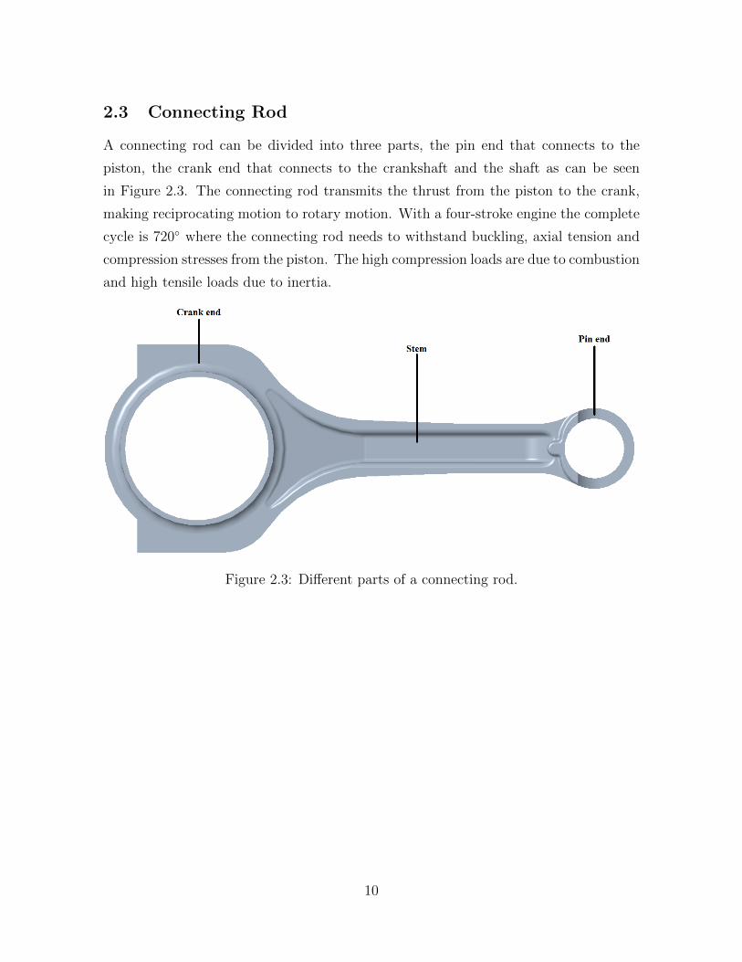
2.3 Connecting Rod
A connecting rod can be divided into three parts, the pin end that connects to the
piston, the crank end that connects to the crankshaft and the shaft as can be seen
in Figure 2.3. The connecting rod transmits the thrust from the piston to the crank,
making reciprocating motion to rotary motion. With a four-stroke engine the complete
cycle is 720◦ where the connecting rod needs to withstand buckling, axial tension and
compression stresses from the piston. The high compression loads are due to combustion
and high tensile loads due to inertia.
Figure 2.3: Different parts of a connecting rod.
10

2.3.1 Forces
The forces acting on the connecting rod and piston can be seen in the free body diagram
in Figure 2.4 and it was used to derive the forces, velocities and accelerations acting on
it.
Figure 2.4: Free body diagram of the piston and connecting rod.
11

By using trigonometric relationships the angular velocity around the pin end seen in
Equation (2.1) was derived and by deriving it the angular acceleration seen in Equation
(2.2) was obtained.
ϕ =rω cos θ
a cosϕ(2.1)
ϕ =1
cosϕ
(−rω2 cos θ
a+ ϕ2 sinϕ
)(2.2)
The forces on the piston in the y-direction can be seen in Equation (2.3) and the
expression for Fp in Equation (2.4).
Fy = −mpy − Fp (2.3)
Fp = PAp (2.4)
The acceleration in x- and y-direction on the connecting rod can be seen in Equation
(2.5) and (2.6) respectively.
ax = bϕ cosϕ− bϕ2 sinϕ (2.5)
ay = y + bϕ sinϕ+ bϕ2 cosϕ (2.6)
In Equation (2.7) the relationship between the forces on the connecting rod in the
y-direction can be seen.
Ty = mcay − Fy (2.7)
12

With the help of forces in x-direction and moment around the center of gravity a matrix
for Fx and Tx can be derived and it can be seen in Equation (2.8).
[1 1
−b cosϕ c cosϕ
][Fx
Tx
]=
[mcax
Iϕ− cTy sinϕ+ bFy sinϕ
](2.8)
To translate the forces, velocities and accelerations to the connecting rods own coordi-
nate system Equation (2.9) were used.
[cosϕ sinϕ
− sinϕ cosϕ
][x
y
]=
[x′
y′
](2.9)
For the full derivation see Appendix A.
The data for the engines pressure cycle for different angular velocity ranging from 1000-
6000 rpm were given and can be seen in Figure 2.5. The data is based on simulations
made by CVUT in Prague.
Figure 2.5: The engines pressure cycle.
13
The mass and geometrical data used can be seen in Table 2.1, the connecting rod length
is the center-center distance of the holes. To acquire the data Hoganas AB had made
reverse engineering on the original connecting rod and measured it with a ZEISS CMM
(Coordinate Measurement Machine).
Table 2.1: Mass and geometrical data.
Piston radius Piston mass Connecting rod mass Connecting rod length Crankshaft length
37,25 mm 0,34 kg 0,34 kg 140,04 mm 40 mm
2.3.2 Buckling
Buckling is important to have in mind when designing a connecting rod due to the
high compression and inertia loads acting on it during a cycle, evermore due to the
force acting on the rod from an angle. The critical load is the value of the axial force
when the conditions go from stable to unstable and failure can occur. The critical
loads corresponds to different order of buckling modes. The higher modes are often of
no interest because the part will break when the load reaches the lowest critical value.
Other than the critical load a factor called Buckling Load Factor, BLF, can be obtained
which is a safety factor against buckling. [6]
2.3.3 Fatigue
Failure caused by fatigue occurs when an object is subjected to a dynamic load repeti-
tively for a large number of cycles. The failure will happen at a lower stress level than if
the force was to be applied statically and the failure starts with a small crack in a point
of high stress, such as in sharp corners or different transition areas. The crack gets
larger until the remaining material cannot withstand the loads and a fracture occurs.
This applies to a connecting rod since the load is dynamic and cyclic and when failure
happens in a connecting rod the engine will most likely brake as well. Therefore when
designing the connecting rod against failure, an infinite life is desired. [6]
With testing of the material it is possible to determine the failure load. The material
is subjected to different stress levels and the amount of cycles to failure is determined.
When enough data is collected it is possible to plot a S-N diagram which shows the
endurance limit.
14
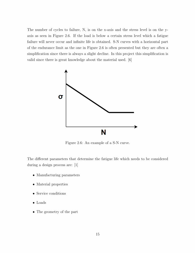
The number of cycles to failure, N, is on the x-axis and the stress level is on the y-
axis as seen in Figure 2.6. If the load is below a certain stress level which a fatigue
failure will never occur and infinite life is obtained. S-N curves with a horizontal part
of the endurance limit as the one in Figure 2.6 is often presented but they are often a
simplification since there is always a slight decline. In this project this simplification is
valid since there is great knowledge about the material used. [6]
Figure 2.6: An example of a S-N curve.
The different parameters that determine the fatigue life which needs to be considered
during a design process are: [1]
• Manufacturing parameters
• Material properties
• Service conditions
• Loads
• The geometry of the part
15
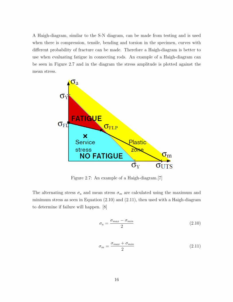
A Haigh-diagram, similar to the S-N diagram, can be made from testing and is used
when there is compression, tensile, bending and torsion in the specimen, curves with
different probability of fracture can be made. Therefore a Haigh-diagram is better to
use when evaluating fatigue in connecting rods. An example of a Haigh-diagram can
be seen in Figure 2.7 and in the diagram the stress amplitude is plotted against the
mean stress.
Figure 2.7: An example of a Haigh-diagram.[7]
The alternating stress σa and mean stress σm are calculated using the maximum and
minimum stress as seen in Equation (2.10) and (2.11), then used with a Haigh-diagram
to determine if failure will happen. [8]
σa =σmax − σmin
2(2.10)
σm =σmax + σmin
2(2.11)
16

When the operating point, P, is obtained and inserted in the Haigh-diagram the prob-
ability of failure can be determined. There will be failure if the point is above the
line and if the point is under the line a safety factor against failure can be determined
according to Equation (2.12).[8]
n =AB
AP(2.12)
Equation (2.12) is used when σm is constant but σa can vary. In Figure 2.8 it can
be seen where point A, B and P are placed. This method of calculating the safety
factor were chosen because it is the most conservative method and therefore will not
overestimated the fatigue strength.[8]
Figure 2.8: A Haigh-diagram with operating point P, point A and B for determining
safety factor.
17

2.3.4 Material
It is crucial to have a combination of cost effective and high performance material to
have a working connecting rod. Since PM materials have pores in them the connecting
rods needs to have martensite structure to improve the strength. The material used to
achieve this is chromium based alloy combined with sinter hardening which gives good
qualities against fatigue and is cost effective e.g. AstaloyTMCrA + 2%Ni + 0.6%C and
Astaloy CrM + 0.45%C.[11]
Astaloy CrA and Astaloy CrM are both water atomised iron powders. Astaloy CrA
contains 1.8% chromium which offers high strength, stable dimensions and good com-
pressibility at a low cost. With the addition of copper or, as in this case, nickel it
enables sinter hardening. The Astaloy CrM contains 3% chromium and 0.5% molyb-
denum which gives it great hardenability. After sintering high strength and hardness
can be achieved. It can be sintered in high temperature and is suitable for sinter
hardening.[4]
The material parameters used for the calculations can be seen in Table 2.2.
Table 2.2: Material data for the concepts.
Density, ρ Young’s Modulus, E Poisson’s ratio, ν
7.15 g/cm2 150 GPa 0.28
18

The Haigh-diagram for Astaloy CrA + 2%Ni + 0.6%C can be seen in Figure 2.9 which
will be used for the fatigue calculations for the concepts. The diagram was constructed
based on data from measurements made by Hoganas AB.
Figure 2.9: A Haigh-diagram for Astaloy CrA + 2%Ni + 0.6%C with 50% probability
of fracture.
19
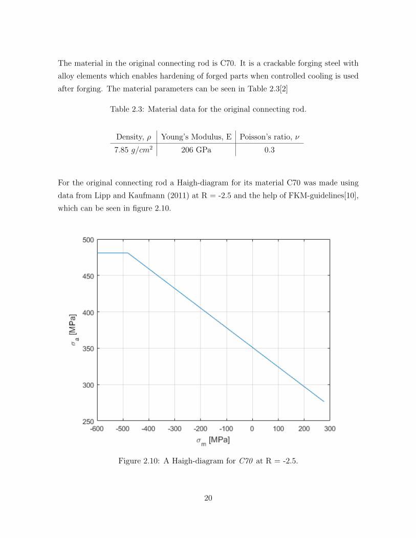
The material in the original connecting rod is C70. It is a crackable forging steel with
alloy elements which enables hardening of forged parts when controlled cooling is used
after forging. The material parameters can be seen in Table 2.3[2]
Table 2.3: Material data for the original connecting rod.
Density, ρ Young’s Modulus, E Poisson’s ratio, ν
7.85 g/cm2 206 GPa 0.3
For the original connecting rod a Haigh-diagram for its material C70 was made using
data from Lipp and Kaufmann (2011) at R = -2.5 and the help of FKM-guidelines[10],
which can be seen in figure 2.10.
Figure 2.10: A Haigh-diagram for C70 at R = -2.5.
20

2.4 Finite Element Analysis
Since the connecting rod has a complex geometry with e.g. different cross section areas
the use of FEA is necessary. It is used to investigate the stresses and displacement to
see if there are any critical areas which need to be redesigned. The obtained stresses
are used to determine the fatigue life and where such failure will happen. The critical
buckling load will also be calculated using FEA.
According to Shenoy and Fatemi (2006) static axial loads are mostly used when design-
ing connecting rods. However they compare with using quasi-dynamic analysis. Since
there are time varying inertia loads the results are different from the two analysis types
and the static giving less realistic values as seen in Figure 2.11. The time varying loads
is introducing bending stresses and axial loads which is varying along the length of the
connecting rod.
The stress range used in a static analysis is the difference between the maximum stress,
which is the maximum tensile force, and the minimum stress, which is the maximum
compressive force. Rather than using the load range at the maximum power output as
in a dynamic analyse. This could result in a connecting rod with a very conservative
design. Another factor discussed is that with a static analysis the model gets over
constrained and this being another factor for the less realistic values.
Figure 2.11: The difference in von Mises stress amplitude in different locations between
static and quasi-dynamic analysis.[12]
21

3 Methodology
This section explains the work process from ideas to finished concepts with the use of
Ulrich and Eppinger’s (2016) product development process.
3.1 Concept generation
The concept generation started with a study of different designs already used for con-
necting rods, both from external sources and also from earlier projects carried out by
Hoganas AB. This resulted in 13 different designs where some were totally different
and some more similar to each other. All the concepts where designed to be able to
manufacture with PM.
3.2 Modeling
The first model created was a base with the right dimensions of the big and small end
which should not be altered between the different concepts. There were no drawing
or CAD-model for the original connecting rod but Hoganas AB had made reverse
engineering of the original for an earlier project where the dimensions were measured.
These measurements were acquired and used in PTC Creo, a CAD software, to create
the base seen in figure 3.1.
Figure 3.1: The base used for the different concepts.
22

As seen in Figure 3.2 representation of the original connecting rod was also done to be
able to benchmark against.
Figure 3.2: The model of the original connecting rod.
The concepts were modeled but after concept screening it resulted in nine concepts
making it to the FEA stage. In the concept screening the concepts were evaluated
against the delimitations and if they did not meet the specification they were eliminated.
During the FEA the iterative process began with the concepts being altered to obtain
the optimal shape and minimize the stress in different areas.
3.3 Finite Element Analysis
The analyse method chosen was a static analysis even though some studies showed
an increase in stress levels compared to a dynamic one. This was done to reduce
computational time and since the objective was to compare different concepts this
simplification will effect all the concepts in the same way. A rigid link was put in both
the small and the big hole to be able to constrain them. This could be done since the
deformation in the ends is not to be examined. The small end was constrained in X
and Z translation. The big end was constrained in all translation direction and X and
Y rotation. The force was applied in the small end, the accelerations, angular velocity
and angular acceleration were applied at the center of gravity as seen in Figure 3.3.
23

Figure 3.3: One of the concepts with the forces and constraints applied.
The mesh was created by using PTC Creo’s built-in system where it iterates, making
higher order mesh for each run until the stresses converge. Then using mesh control to
be able to control the size of the elements in critical areas.
To make the scoring process the nine remaining concepts were analysed once to see if
they met the specification in regards to stress levels. Three concepts did not make it
past the scoring due to high stress concentrations and the need for large alterations
resulting in overweight or not manufacturable solutions.
The different load cases which were tested were:
• Maximum Compressive Force
• Maximum Tensile Force
• Maximum Angular Velocity
• Maximum Angular Acceleration
• Maximum Acceleration in x-direction
The maximum acceleration in y-direction was neglected due to its small impact on the
connecting rod and in Appendix B the table with the input data can be seen.
24

The results were evaluated for the normal stress in y-direction and critical areas where
risk of failure was determined for the different concepts. The areas and the stress data
can be seen in Appendix C which were then used for the fatigue evaluation. The number
of critical areas varies depending on concept.
For the buckling analysis a single compressive load of 1 kN was applied at the small
end with the same constraints. This results in the value on the Buckling Load Factor
being the amount of force in kN the connecting rod can withstand before any buckling
will occur.
3.4 Manufacturing ranking
For the manufacturing ranking the parameters that will have impact are the number
of punches, punch levels, if there is a tapered geometry, how long the tapering is and
number of radii. For the ranking the radii at the small and the big hole were neglected
since it is the same for all concepts. The rating were made somewhat subjectively.
The number of rods manufactured per hour will be determined theoretically by evalu-
ating how difficult the filling of the cavity is. It is also assumed that the press is in line
with the sintering furnace so the press can feed the furnace directly with components.
25

4 Results
In this section the final concepts, results of the stress analysis and manufacturing rating
are presented.
4.1 Concepts
In Figure 4.1 the first concept named Plus is seen and the design can be described as
an inverted I-beam with thicker sections were the I-beam has thinner sections and vice
versa.
Figure 4.1: Concept 1: Plus.
The second concept named Tapered + I can be seen in Figure 4.2 and it is a concept
which can be described as tapered I-beam. The stem is tapered with a cavity to lower
the weight without compromising the height or thickness.
Figure 4.2: Concept 2: Tapered + I.
26

The next concept named I-Beam + Tapered can be seen in figure 4.3 and it closely
resembles the original but redesigned to be PM friendly. The cavity has a tapered part
to minimize the number and size of radii.
Figure 4.3: Concept 4: I-Beam + Tapered.
In Figure 4.4 the concept named Hole can be seen. The stem is completely flat and
therefore very PM friendly. It has holes to reduce the weight without introducing any
radii or tapered sections.
Figure 4.4: Concept 5: Hole.
27

Tapered Round can be seen in Figure 4.5 and to try to counteract the problem with the
tapered design where one end of the stem becomes thin, this concept has the thinnest
part in the middle. The roundness in the tapered area is to avoid sharp transitions to
minimize stress concentrations.
Figure 4.5: Concept 7: Tapered Round.
The last concept named Tapered can be seen in Figure 4.6. The stem of this concept
is tapered which eliminates any use of radii but the stem get thin at the big eye.
Figure 4.6: Concept 14: Tapered.
The rejected concepts can be seen in Appendix D.
28

4.2 Fatigue
The values of the stress amplitude and the mean stress can be seen in Table 4.1 and
the points plotted in the Haigh-diagram are found in Appendix E.
Table 4.1: Stress amplitude and mean stress in different locations on the connecting
rods. The results are given in MPa.
1 2 3 4 5 6
Original
σa 221,760 221,785 171,320 198,705 196,740 -
σm -183,640 -172,515 -158,980 -171,795 -126,560 -
Concept 1 (Plus)
σa 146.895 152.840 170.760 146.790 153.373 163.035
σm -190.805 -161.560 -141.240 -198.910 -160.826 -131.665
Concept 2 (Tapered + I)
σa 241,545 210,855 197,250 178,850 180,005 -
σm -194,955 -197,045 -169,650 -134,450 -148,695 -
Concept 4 (I-Beam + Tapered)
σa 150,420 164,706 154,544 193,590 147,238 151,110
σm -138,080 -167,293 -157,155 -96,110 -144,961 -106,390
Concept 5 (Hole)
σa 226,955 207,788 201,150 186,620 211,615 221,385
σm -148,245 -202,511 -154,550 -156,080 -196,185 -142,815
Concept 7 (Tapered Round)
σa 168,160 203,565 189 139,045 - -
σm -142,040 -152,235 -85,60 -114,455 - -
Concept 14 (Tapered)
σa 204,550 205,265 138,250 177,615 - -
σm -146,050 -137,235 -108,950 -80,385 - -
29

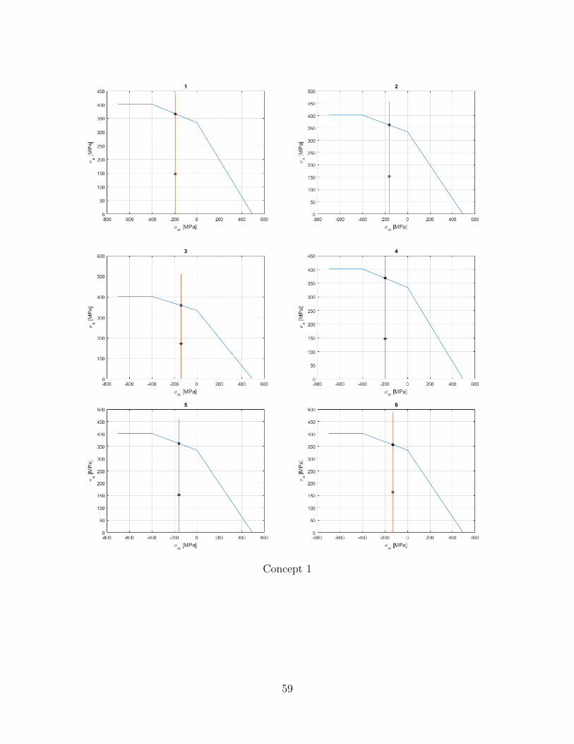
All the concepts had their stress in the safe zone in the Haigh-diagram and their cal-
culated safety factor can be seen in Table 4.2.
Table 4.2: Safety factor in the different critical areas, lowest safety factor are bold.
1 2 3 4 5 6
Original 1,81 1,79 2,30 2,00 1,96 -
Concept 1 (Plus) 2,49 2,36 2,10 2,51 2,36 2,19
Concept 2 (Tapered + I) 1,52 1,74 1,84 2,0 2,0 -
Concept 4 (I Beam + Tapered) 2,38 2,20 2,33 1,81 2,44 2,33
Concept 5 (Hole) 1,58 1,77 1,79 1,93 1,74 1,62
Concept 7 (Tapered Round) 2,13 1,77 1,84 2,54 - -
Concept 14 (Tapered) 1,75 1,74 2,55 1,96 - -
4.3 Buckling
The results of the buckling load factor from the analysis are presented in Table 4.3. The
result is the amount of compressive force in kN the connecting rod can withstand before
it buckles. Each results correspond to one buckling mode, from a practical standpoint
the first is of interest since it will break before reaching the higher order of modes.
Table 4.3: The Buckling Load Factors for the different concepts and the first factor in
comparison with the original in percent.
1 % 2 3
Original 402,26 1 556,59 825,2
Concept 1 (Plus) 346,37 0,86 466,97 842,56
Concept 2 (Tapered + I) 354,67 0,88 684,24 808,56
Concept 4 (I-Beam + Tapered) 499,29 1,24 654,88 675,78
Concept 5 (Hole) 373,22 0,93 537,64 618,43
Concept 7 (Tapered Round) 325,33 0,81 485,35 809,63
Concept 14 (Tapered) 198,51 0,49 794,91 1059,25
30

In Figure 4.7 the different modes can be seen for concept 14. In which direction the
first mode buckles is depending on the design and the first mode might buckle around
the x-axis rather the z-axis as this concepts does.
Figure 4.7: The three modes for concept 14.
31
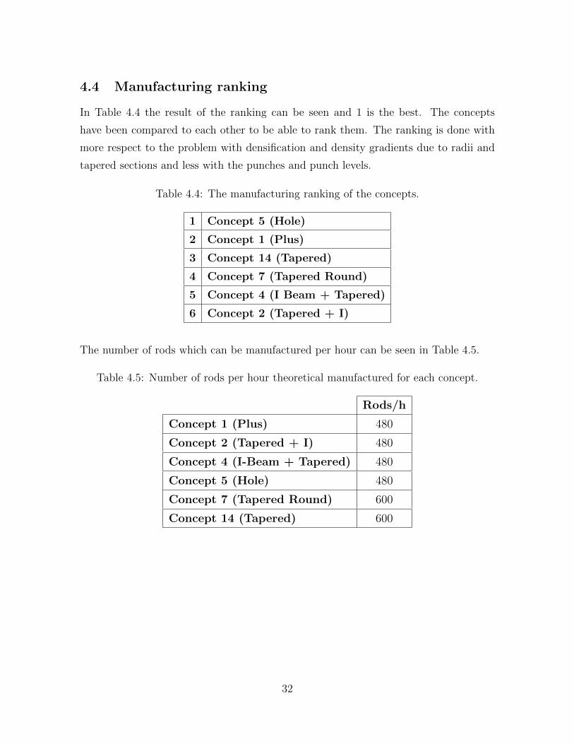
4.4 Manufacturing ranking
In Table 4.4 the result of the ranking can be seen and 1 is the best. The concepts
have been compared to each other to be able to rank them. The ranking is done with
more respect to the problem with densification and density gradients due to radii and
tapered sections and less with the punches and punch levels.
Table 4.4: The manufacturing ranking of the concepts.
1 Concept 5 (Hole)
2 Concept 1 (Plus)
3 Concept 14 (Tapered)
4 Concept 7 (Tapered Round)
5 Concept 4 (I Beam + Tapered)
6 Concept 2 (Tapered + I)
The number of rods which can be manufactured per hour can be seen in Table 4.5.
Table 4.5: Number of rods per hour theoretical manufactured for each concept.
Rods/h
Concept 1 (Plus) 480
Concept 2 (Tapered + I) 480
Concept 4 (I-Beam + Tapered) 480
Concept 5 (Hole) 480
Concept 7 (Tapered Round) 600
Concept 14 (Tapered) 600
32

5 Discussion
In this section the results of the fatigue, buckling and manufacturing ranking will be
discussed. The choice of FEA-method will also be addressed.
5.1 Buckling
All the concepts, except for number 4, perform worse than the original. This is expected
since the I-beam shape of the original is known to counteract buckling well. Concept 14
performs the worst against buckling of all the concepts and will only withstand half of
the force before buckling compared to the original, but it will not buckle under normal
loading conditions for this engine since maximum force is 38.5 kN. This result is also
expected due to its narrow geometry on the stem and because the thickness varies.
This buckling result is a good indicator that a simpler geometry, that will be more PM
friendly, could be a good option for a connecting rod.
If this would be a study to determine the best design for this exact engine, the buckling
analysis could be done with a real extreme value for the loads and a safety factor would
be the result. The method used in this study for the buckling analysis is beneficial in a
comparison study where the results will act as guidelines for choosing design regardless
of which engine. This is since it gives a buckling load factor which easier can be used
for another load cycle without needing to re-simulate the designs.
5.2 Fatigue
When comparing the safety factors the lowest ones are the most interesting to compare
but another factor to consider is the range of the safety factors for each concept and to
have in mind the number of critical areas. Even if a concept has a low safety factor in
one area, the fact that there are less critical areas could be beneficial in an improvement
standpoint. There are two ways to calculate the safety factor for this case, the one used
with the stress amplitude varies and one where both the stress amplitude and mean
stress varies proportionally. To know which one to choose in this case, a more in depth
study would be needed so the decision were made that both were investigated. The one
presented in this paper were the more conservative and therefore used since it will not
overestimate the fatigue life. Since the model of the original is only a representation
33

and not an exact copy the fatigue results and its safety factor should not be interpreted
as the real value, only as an approximation to compare the concepts with. One other
factor to have in mind is that the Haigh-diagram for the concepts are constructed with
a 50% probability of fracture.
There are problems with the design of the transitions on the connecting rod when
designing a PM friendly one. This is due to the fact that to counteract the stress
concentrations, smooth transitions is desirable, large radii are good but with PM small
radii are more beneficial for manufacturing. With large radii there can be problem in
the densification and resulting in less density in the middle, which can lead to failure.
Because of this, large radii which can be seen in a forged connecting rod is possible with
PM but might be worse than small radii since it may lead to less control of the density.
All of this effects the fatigue results and is needed to have in mind when evaluating the
concepts for improvements in this regard.
5.2.1 Concept 1
This concept has the highest safety factor of all the concepts and even higher than the
original. The most problematic areas are in the transition from the big end to the stem
which were expected since the radii are the smallest there and on the stem close to the
small end. Even though there were six problematic areas recognized, the safety factors
are high enough to say that the number of areas is not something negative in this case.
To improve the concept the first thing would be to look into the radii and see if there
were any that could be redesigned against fatigue better without compromising the
manufacturing. Another thing could be to look into the width of the stem part that
protrudes in z-direction and see if that would improve the concept.
5.2.2 Concept 2
Concept 2 has the lowest safety factor but only in one area. Otherwise it performs
similar to the other concepts. The area is the outside of the stem, at the transition
to the large end where its design is the most narrow. It was expected to have a lower
safety factor here since the radius is smaller than the other one without the tapered
stem but the fact that it is lower here than in the cavity was not expected.
34
With another radius on the stem in the transition to the big end the problem with the
high stress in this area could be solved. It would be wise to also investigate if there
could be anything done in the cavity at the big end to make the design even better
resulting in a design which would perform better against fatigue.
It is positive that the transition at the small end performs well against fatigue and it
seems that little to no redesign is needed.
5.2.3 Concept 4
This concept is placed in the middle in regards to the safety factor and the area with
the lowest safety factor being in the stem where the tapering ends and the flat section
begins. There were six areas recognized as problematic but the safety factor of all but
the lowest is above the original. This concept performs well against fatigue. Most of
the concepts problem areas are at or around the cavity at the big end as expected
since the shape at the small end is relatively uniform. The radii to the small end were
investigated but with such high safety factor it should not be a problem.
The biggest issue is the transition from the tapered section to the flat section and it
could be wise to investigate if it can be made better in regard to fatigue. Even though
there were six identified problematic areas, it would not be a problem from a fatigue
standpoint for five of them.
5.2.4 Concept 5
The biggest problem with this concept from a fatigue standpoint is in the holes which
makes this concept one of the worst. The lowest safety factors are found in the lower
hole and overall there are six investigated areas where the lowest ones are connected
to the holes. In the transition to the small end there seems to be a high enough safety
factor not to have a fatigue problem.
The shape of the lower hole should be investigated to try to obtain a better shape to
increase the safety factor and also the width of the top hole to see if that will effect the
safety factor.
35

5.2.5 Concept 7
This was one of the better against fatigue with a relative high safety factor and there
were also only four problematic areas found where two of them seem to be not a problem.
There is no problem at the transitions, either to the big or small end, but at the thinnest
part of the stem.
This concept performed well against fatigue and the only problematic area to investigate
further is the shape and thickness of the stem. The stem might perform better with a
thicker stem or a different radius on the roundness of it.
5.2.6 Concept 14
With the tapered design of this concept there is no high stresses at the small end
therefore all problematic areas are at the big end. The lowest safety factor is in the
middle of all the concepts but the fact that there are only four areas identified and two
of them are close together this design relatively good against fatigue.
To be able to make this design better the stem width could be investigated as well as
the big transition radii going from the big end to the stem. At area 3 there is a stress
concentration which will not be a problem for the fatigue but could be investigated for
a better design.
5.3 Finite Element Analysis
The choice of a static FEA-method serves its purpose in this study since it is a qual-
itative study which compares the different concepts. If the values on the stress would
have been the most important value, a dynamic method would be preferable since it
will yield more realistic results. With the constraints used on the small and the big
hole on the models, where they are not allowed to deform, is another factor that will
effect the stress if the goal is to get more realistic values. Since those ends were not
to be examined in this paper it was a valid simplification to save computational time.
Therefore the stress values in this paper should not be taken as absolute, rather as a
comparative study.
36

5.4 Manufacturing ranking
Here follows an explanation about the difference in the concepts and why they got
their ranking. This ranking is somewhat subjective and might not reflect how all
manufacturers perceive manufacturing difficulties. It was made with the help of Thomas
Schmidtseifer[13] who is an expert in PM manufaturing. This is due to for example
the individual equipment available at part makers since if they only have a two level
machine they will not like a three level part, therefore ranking it lower. Therefore
this ranking is done with more respect to the problem with densification and density
gradients and less with the punches due to the different equipment available. The small
and the big end will not be discussed since it is not in the scope for this paper. They
are the same for all the concepts.
5.4.1 Concept 1
This concept requires five punches on three punch levels to manufacture and can be
described as an inverted I-beam, where the stem sections are thin where the I-beam is
thicker and vice versa. This will benefit in the manufacturing process since there will be
no problem with density gradients due to tapering. The main problem in manufacturing
for this concept will be the radii in the transitions to the stem. This is due to in PM
it is beneficial to have as small radii as possible because of larger radii give density
gradient which compromise the strength of the connecting rod.
5.4.2 Concept 2
This concept requires three punches on three punch levels to manufacture and is a type
of I-beam with a tapered stem. This design will have problems with density gradients
both due to the tapered stem but also due to the radii in the cavity of the stem. The
inner radii are needed to be able to avoid stress concentration but it results in a more
difficult design to manufacture.
5.4.3 Concept 4
This concept reassembles the original the most with a version of an I-beam and it
requires four punches on three levels. The beneficial with this compared to the original
is the tapering in the cavity which eliminates an inner radius but it adds another difficult
37
section to manufacture. On the other hand the other inner radii can be relatively small
which benefits the design in less for risk density gradients.
5.4.4 Concept 5
This concept requires three punches on two punch levels. The use of rods for the holes
removes the need to use an extra punch which is needed when making a cavity or
similar designs. With the hole design it is possible to lower the weight without making
a more complex design. This results in a flat, no tapered section, minimum use of radii
and therefore a relatively easy design to manufacture. The shape of the lower hole in
this design is the most difficult to manufacture since it is a rather complex geometry
compared to a normal hole.
5.4.5 Concept 7
The geometry of this concept is tapered but with a round shape instead of a straight
curve. It needs again three punches on two punch levels to manufacture and it eliminates
the need of radii on the stem. The main manufacturing problem with this design is
to obtain the round tapering with minimum density gradients to not compromise the
strength.
5.4.6 Concept 14
This concept has a tapered stem with no cavity or radii, it needs two punches on two
punch levels to manufacture, which is the lowest of all the concepts. With no need
for radii the only problem with this is the thickness and length of the tapered section,
which will give problem in the densification of the powder.
5.4.7 Justification of the ranking
Concept 5 ranks the best due to the need for only three punches, zero tapered sections
and radii, the holes are made with rods which are there from the beginning. Concept
1 comes before concepts 7 and 14 even though it needs five punches and the other two
only need three and two punches respectively. This is because it does not have any
tapered section, it has more radii but that does not impact densification of the powder
and the manufacturing as much as a tapering does. The number of punches for concept
38

7 (three punches) and 14 (two punches) is different and the tapering on 14 gives bigger
density variations. Therefore concept 7 ranks higher.
The two concepts ranking in the bottom are 2 and 4. They both need three and
four punches respectively and have tapered sections. Concept 4 has a more complex
geometry than 2 which makes the manufacturing more difficult but gives less density
variations. Therefore it ranks higher.
The amount of rods per hour is not included in the ranking since it is based on an
optimal manufacturing process with no problem in the process.[13]
39
6 Conclusions
For this master thesis the objective was to evaluate different design for pressed and
sintered connecting rods, the conclusions from this study are as follow:
• Buckling will not be an issue for the concepts since from the buckling analysis
the conclusion can be drawn that none of the concepts will buckle under the
engine cycle given for this specific case. Even though there are differences in the
Buckling Load Factor and the majority of the concept performs worse than the
original connecting rod, the worst one still has a safety factor of 5.
• From the fatigue results there is evidence that a single press and sintered
connecting rod is possible.
• The concepts with long tapered sections, concept 4, 7 and 14, have their highest
stress concentration on their sides due to their stem being thinner and compression
occurs in the material in that area.
• The concepts with radii and short tapering experience their stress concentrations
in the transition areas.
• The biggest issue in the manufacturing of connecting rods is to control the density
since the need of large radii and tapered section or just one of them. There are
clear differences and difficulties in the manufacturing of the concepts which will be
beneficial for different manufactures depending on their equipment as mentioned
in the discussion part.
The conclusions above do not mention any concept as the best one since this study is
a evaluation to be used as a basis for future connecting rod studies. This is because
material, application and manufacturer may affect which design is the best one. The
study will help and minimize the time spent to make the decision on which design to
move forward with.
40
7 Future work
In order to improve this study the following things can be done:
• Use a different FEA-method and investigate how the stresses behave e.g. use a
dynamic analysis instead of a static one.
• Evaluate the stresses in the big and small end in order to have a complete stress
analysis.
• Investigate the problematic areas mentioned in the discussion to further improve
the concepts.
• Make a more detailed manufacturing comparison with a rating rather than ranking
where every manufacturing parameter is more closely evaluated.
41

References
[1] Afzal, Adila. 2004. Fatigue Behaviour and Life Predictions of Forged Steel and Powder Metal
Connecting Rods, The university of Toledo.
[2] Dale, James R. 2005. Connecting Rod Evaluation, Metal Powder Industries Federation.
[3] Ulrich, Karl T and Eppinger, Steven D. 2016. Product Design and Development. 6th edition.
New York, NY: McGraw-Hill Education.
[4] Hoganas AB. 2013. Hoganas Handbook for Sintered Components 1-3.
[5] Chasoglou, Dimitris and Bergman, Ola. 2017. Sinter hardening material solutions for high
performance applications.
[6] Gere, James M. 2004. Mechanics of Materials. 6th edition. London: Thomson Learning.
[7] Ekberg, Anders. High Cycle Fatigue (HCF) part II, Chalmers
http://www.am.chalmers.se/~anek/teaching/fatfract/98-6.pdf (2019-16-05)
[8] Lundh, Hans. 2016. Grundlaggande hallfasthetslara. Lund: Studentlitteratur AB.
[9] Lipp, Klaus and Kaufmann, Heinz. 2011. Schmiede- und Sinterschmiedewerkstoffe fur PKW-
Pleuel. Springer Automotive Media C Vol. 72, nr. 5: 416–421. DOI: 10.1365/s35146-011-0096-1
[10] Forschungskuratorium Maschinenbau. 2003. Analytical strength assessment of components in
mechanical engineering : FKM-guideline. 5th edition. Frankfurt: VDMA Verl.
[11] Andersson, Michael and Larsson, Caroline. 2016. Cost Effective PM Connecting Rod Concept.
[12] Shenoy, P S and Fatemi, A. 2006. Dynamic analysis of loads and stresses in connect-
ing rods. Proc. IMechE Journal of Mechanical Engineers Vol. 220, part C: 615-624. DOI:
10.1243/09544062JMES105
[13] Thomas Schmidtseifer Manager Market Development & Customer Projects Hoganas AB,
e-mail February-June 2019
42

A Derivation
With the help of Figure 2.4 and trigonometric relations the equations were derived.
The distance, velocity and acceleration of the connecting rod can be seen in Equation
(A.1)-(A.5).
y = a cosϕ+ r cos θ (A.1)
y = −aϕ sinϕ− rθ sin θ (A.2)
θ = ω (A.3)
⇒ y = −aϕ sinϕ− rω sin θ (A.4)
y = −aϕ sinϕ− aϕ2 cosϕ− rω2 cos θ (A.5)
The velocity and acceleration of the connecting rods angle of obliquity were derived in
Equation (A.6)-(A.10).
sinϕ
r=
sin θ
a(A.6)
ϕ cosϕ
r=ω cos θ
a(A.7)
⇒ ϕ =rω cos θ
a cosϕ(A.8)
ϕ cosϕ− ϕ2 sinϕ
r=−ω2 cos θ
a(A.9)
⇒ ϕ =1
cosϕ
(−rω2 cos θ
a+ ϕ2 sinϕ
)(A.10)
43

Distance, velocity and acceleration of centre of gravity is expressed in Equation (A.11)-
(A.16).
xg = b sinϕ (A.11)
xg = bϕ cosϕ (A.12)
xg = ax = bϕ cosϕ− bϕ2 sinϕ (A.13)
yg = y = b cosϕ (A.14)
yg = y + bϕ sinϕ (A.15)
yg = ay = y + bϕ sinϕ+ bϕ2 cosϕ (A.16)
Force in the y-direction in the piston can be calculated using Equation (A.17)-(A.19).
mpy + Fp + Fy = 0 (A.17)
⇒ Fy = −mpy − Fp (A.18)
Fp = PAp (A.19)
Force in the y-direction in the connecting rod can be calculated using Equation (A.20)
and (A.21).
Fy + Ty −mcay = 0 (A.20)
⇒ Ty = mcay − Fy (A.21)
44
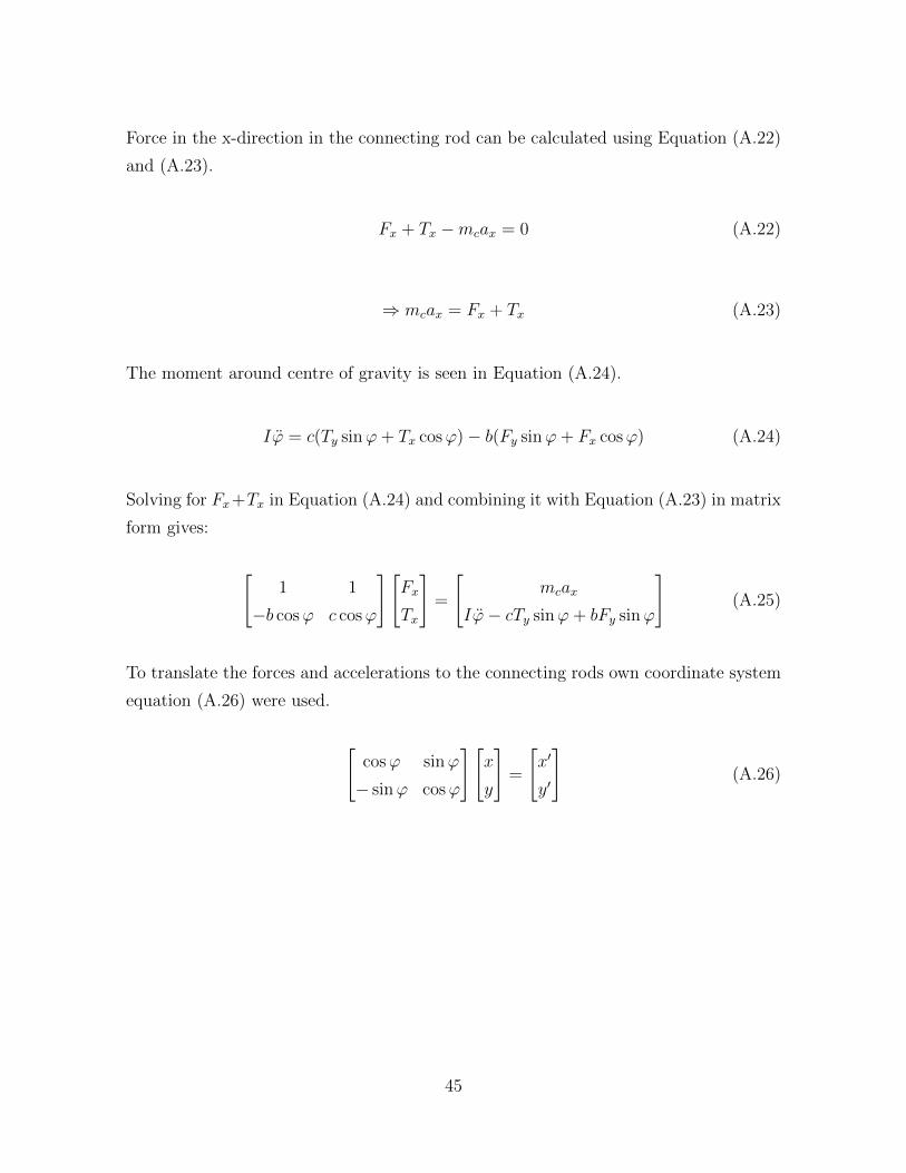
Force in the x-direction in the connecting rod can be calculated using Equation (A.22)
and (A.23).
Fx + Tx −mcax = 0 (A.22)
⇒ mcax = Fx + Tx (A.23)
The moment around centre of gravity is seen in Equation (A.24).
Iϕ = c(Ty sinϕ+ Tx cosϕ)− b(Fy sinϕ+ Fx cosϕ) (A.24)
Solving for Fx+Tx in Equation (A.24) and combining it with Equation (A.23) in matrix
form gives:
[1 1
−b cosϕ c cosϕ
][Fx
Tx
]=
[mcax
Iϕ− cTy sinϕ+ bFy sinϕ
](A.25)
To translate the forces and accelerations to the connecting rods own coordinate system
equation (A.26) were used.
[cosϕ sinϕ
− sinϕ cosϕ
][x
y
]=
[x′
y′
](A.26)
45

B Data for FEA
Max comp. force Max tensile force Max ang. vel. Max ang. acc. Max ax
N = 3500, θ = 27◦ N = 6000, θ = 342◦ N = 6000, θ = 0◦ N = 6000, θ = 175◦ N = 6000, θ = 19◦
Concept 1
(Plus)
Force (N) -38515 5464 -9849.2 -7010.54 -33483
Ang. vel (rad/s) 94.0764 171.3582 179.4483 -178.8459 170.4340
Ang. acc (rad/s2) -3.3323e4 -1.1027e5 -1.1291e5 1.1317e5 -1.0437e5
ax (m/s2) -3.789e3 -0.8409e4 -1.0359e4 1.0755e4 -1.1309e4
ay (m/s2) -4.5459e3 -1.7677e4 -1.7394e4 1.3819e4 -1.4854e4
Concept 2
(Tapered H)
Force -38516 5467 -9849.1 -7010.54 -33485
Ang. vel 94.0764 171.3582 179.4734 -178.8459 170.434
Ang. acc -3.3323e4 -1.1027e5 -1.1291e5 1.1317e5 -1.0437e5
ax -3.7034e3 -0.8125e4 -1.0069e4 1.0464e4 -1.1046e4
ay -4.5686e3 -1.7753e4 -1.7476e4 1.3737e4 -1.4929e4
Concept 4
(H-Beam + Tapered)
Force -38515 5465 -9970.9 -7010.6 -33482
Ang. vel 94.0764 171.3582 179.4734 -178.8459 170.4340
Ang. acc -3.3323e4 -1.1027e5 -1.1277e5 1.1317e5 -1.0437e5
ax -3.6847e3 -0.8063e4 -1.0094e4 1.0401e4 -1.0982e4
ay -4.5736e3 -1.7769e4 -1.7419e4 1.3719e4 -1.4945e4
Concept 5
(Hole 1)
Force -38515 5464 -9970.9 -7010.54 -33482
Ang. vel 94.0764 171.3582 179.4734 -178.8459 170.4340
Ang. acc -3.3323e4 -1.1027e5 -1.1277e5 1.1317e5 -1.0437e5
ax -3.7324e3 -0.8221e4 -1.0256e4 1.0563e4 -1.1131e4
ay -4.5609e3 -1.7727e4 -1.7373e4 1.3765e4 -1.4904e4
Concept 7
(Tapered Round)
Force -38516 5465 -9970.9 -7010.4 -33483
Ang. vel 94.0764 171.3582 179.4734 -178.8459 170.4340
Ang. acc -3.3323e4 -1.1027e5 -1.1291e5 1.1317e5 -1.0437e5
ax -3.7747e3 -0.8361e4 -1.0399e4 1.0706e4 -1.1264e4
ay -4.5497e3 -1.7690e4 -1.7332e4 1.3805e4 -1.4867e4
Concept 14
(Tapered)
Force -38515 5465 -9970.9 -7010.5 -33482
Ang. vel 94.0764 171.3582 179.4734 -178.8459 170.4340
Ang. acc -3.3323e4 -1.1027e5 -1.1277e5 1.1317e5 -1.0437e5
ax -3.6754e3 -0.8033e4 -1.0063e4 1.0369e4 -1.0953e4
ay -4.5761e3 -1.7777e4 -1.7428e4 1.371e4 -1.4953e4
Original
Force -38515 5451 -9970.9 -7014 -33470
Ang. vel 94.0764 171.3582 179.4734 -178.8459 170.4340
Ang. acc -3.3323e4 -1.1027e5 -1.1291e5 1.1317e5 -1.0437e5
ax -3.7516e3 -0.8285e4 -1.0321e4 1.0628e4 -1.1191e4
ay -4.5559e3 -1.771e4 -1.7354e4 1.3783e4 -1.4887e4
46

C Stress data from FEA
1 2 3 4 5 6
Concept 1
(Plus)
(X: -53,27,
Y: 10,43, Z: 0)
(X: -42,36,
Y: 3,93, Z: 5,4)
(X: -42,36,
Y: 3,93, Z: -5,33)
(X: -90,92,
Y: 8,81, Z: 0)
(X: -118,58,
Y: 8,12, Z: 2,61)
(X: -111,74,
Y: 3,09, Z: 6,47)
Max Comp. -306,6 -314,4 -312 -302,6 -311,3 -294,7
Max Tensile -43,91 -8,72 29,52 -52,12 -7,453 31,37
Max ang. vel. -164,8 -122,6 -92,71 -176 -132,3 -86,85
Max ang. acc. -166,4 -130,5 -92,9 -176 -132,4 -86,68
Max ax -337,7 -310,5 -282 -345,7 -314,2 -267,4
Concept 2
(Tapered + H)
(X: -42,3,
Y: 6,1, Z: 0)
(X: -38,89,
Y: -0,51, Z: 4)
(X: -39,47,
Y: 3,2, Z: 6,5)
(X: -116,38,
Y: 0,35, Z: 4,07 )
(X: -115,94,
Y: 5,89, Z: 8,44)(X: , Y: , Z: )
Max Comp. -409,9 -407,9 -353,7 -313,3 -328,7 -
Max Tensile -42,04 13,81 -30,7 44,4 31,31 -
Max ang. vel. -205,3 -141,8 -152,2 -78,4 -10,1 -
Max ang. acc. 46,59 -22,58 27,6 -56,87 -36,72 -
Max ax -436,5 -362,8 -366,9 -261,5 -299,8 -
Concept 4
(H Beam + Tapered)
(X: -55,15,
Y: 10,18, Z: 4,78)
(X: -31,50,
Y: 3,48, Z: 2,02)
(X: -48,59,
Y: 6,72, Z: 2,07)
(X: -55,11,
Y: 3,17, Z: 2)
(X: -119,65,
Y: 7,05, Z: 6,44)
(X: -53,87,
Y: -10,31, Z: 3,17)
Max Comp. -286,9 -332 -311,7 -289,7 -292,2 -257,5
Max Tensile -13,66 -2,587 -2,611 11,26 2,277 44,72
Max ang. vel. -128,5 -118,2 -126,4 97,48 -96,54 -45,92
Max ang. acc. 12,34 -12,26 -3,265 -19,8 -26,5 -71,71
Max ax -288,5 -312,5 -306,3 -277,3 -272,4 -203,3
Concept 5
(Hole)
(X: -111,91,
Y: -2,5, Z: -3,2)
(X: -111,9,
Y: 2,5, Z: 3,11)
(X: -119,99,
Y: -7,84, Z: -6,42)
(X: -119,98,
Y: 7,86, Z: 6,42)
(X: -32,38,
Y:-8, Z: 3,19)
(X: -32,33,
Y: 8, Z: 3,17)
Max Comp. -375,2 -366,9 -355,7 -342,7 -362,7 -364,2
Max Tensile 78,71 5,277 46,6 30,54 -33,18 78,57
Max ang. vel. -61,23 -164,5 -80,01 -10,33 -180,5 -75,86
Max ang. acc. -112,6 -4,527 -89,73 -23,47 15,43 -98,78
Max ax -273,9 -410,3 -290,9 -325,1 -407,8 -240,9
Concept 7
(Tapered Round)
(X: -78,
Y: 7,14, Z: 3,6)
(X: -82,85,
Y: 9,1, Z: -3,63)
(X: -120,
Y: 5,76, Z: -6,2)
(X: 120,
Y: 5,29, Z: 6,27)(X: , Y: , Z: ) (X: , Y: , Z: )
Max Comp. -308 -324,3 -274,6 -253,5 - -
Max Tensile -2,898 -45 2,64 24,59 - -
Max ang. vel. -130,5 -176,3 103,4 -76,68 - -
Max ang. acc. 26,12 51,33 -5,195 -29,81 - -
Max ax -310,2 -355,8 -241,7 -231 - -
Concept 14
(Tapered)
(X: -49,88,
Y: 5,33, Z: -3,36)
(X: -46,78,
Y: 5,5, Z: -7,05)
(X: -28,7,
Y: 0,24, Z: -6,44)
(X: -47,03,
Y: -5,45, Z: -3,46)(X: , Y: , Z: ) (X: , Y: , Z: )
Max Comp. -303,3 -307,1 -247,2 -258 - -
Max Tensile -59,58 -47,16 29,3 97,23 - -
Max ang. vel. -185,1 -179,1 -67,36 -7,5 - -
Max ang. acc. 58,5 68,03 -39,29 -132,4 -
Max ax -350,6 -342,5 -218,8 -161,1 - -
Original(X: -115,87,
Y: 0,875, Z: -1,42)
(X: -116,38,
Y: 0, Z: 1,45)
(X: -122,14,
Y: 8,78, Z: -3,17)
(X: -91,39,
Y: 8,79, Z: -6,3)
(X: -91,39,
Y: -8,76, Z: -3,24)(X: , Y: , Z: )
Max Comp. -405,4 -394,3 -330,3 -350 -323,3 -
Max Tensile 38,12 49,27 12,34 -27,24 70,18 -
Max ang. vel. -123,7 -89,64 -107,8 -168,7 -55,93 -
Max ang. acc. -50,71 -64,3 -18,52 26,91 -92,89 -
Max ax -365,9 -344,5 -310,8 -370,5 -261,6 -
The following figures shows where on the concepts the stress were measured.
47

Original
48

Concept 1 (Plus)
49

Concept 2 (Tapered + I)
50
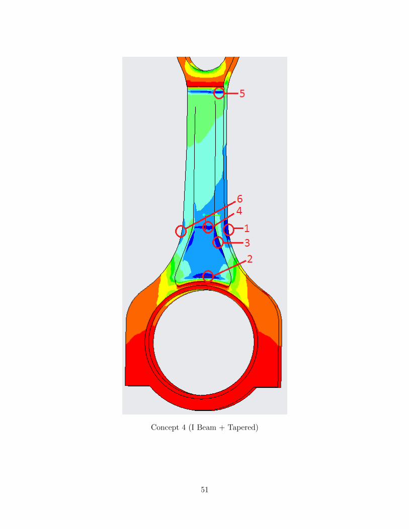
Concept 4 (I Beam + Tapered)
51

Concept 5 (Hole)
52

Concept 7 (Tapered Round)
53

Concept 14 (Tapered)
54
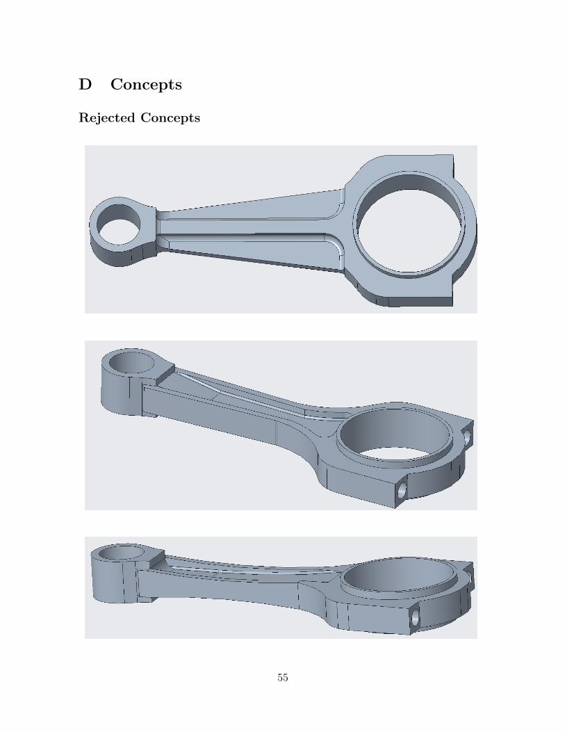
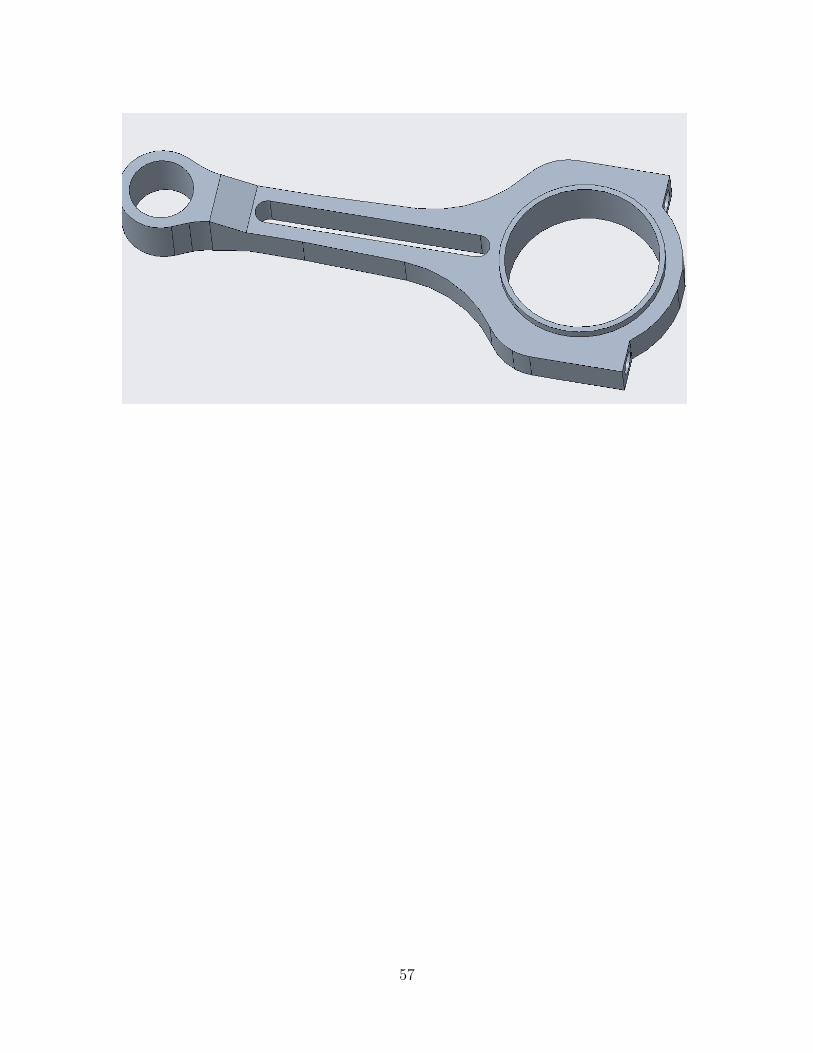
D Concepts
Rejected Concepts
55

56
57

E Critical points in Haigh-diagram
Original
58
Concept 1
59

Concept 2
60

Concept 4
61

Concept 5
62

Concept 7
63

Concept 14
64