EVALUATION OF CONTINGENCY ALLOCATION … Bakhshi... · 20.06 Automobile parking multi-story...
15
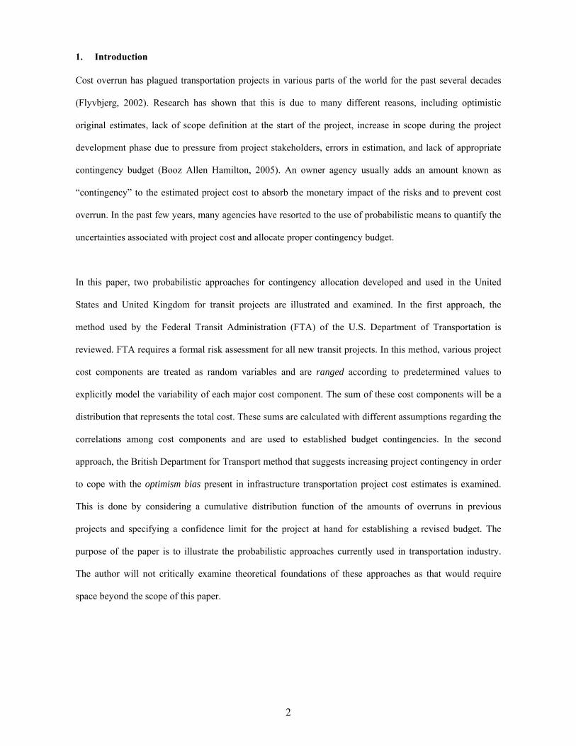
1 EVALUATION OF CONTINGENCY ALLOCATION METHODS FOR TRANSIT PROJECTS IN THE U.S. AND U.K. Payam Bakhshi, Ph.D. Assistant Professor, Department of Construction Management, Wentworth Inst. of Tech. 550 Huntington Ave., ANXSO 008-F, Boston, MA 02115, USA [email protected] Abstract In this paper, two probabilistic approaches for contingecy budget calculation developed and used in the United States and United Kingdom are compared. In the first approach, the method used by the Federal Transit Administration (FTA) of the U.S. Department of Transportation is reviewed. This approach is based upon a range estimating concept. In the second approach, the method applied by the British Department for Transport (DfT) is analyzed. The DfT suggests increasing project contingency in order to cope with the optimism bias in infrastructure transportation projects. This approach relies on cumulative distribution function (CDF), developed by considering historical projects in the same category. This paper evaluates these two methods and makes a quantitative comparison of the results obtained by these methods. This is accomplished by analyzing the cost performance data of a group of major transit projects in the U.S., applying the two methodologies, and comparing and analyzing the results. The problem areas of these approaches are discussed and recommendations are made to optimize the use of these techniques. The paper will be useful for owner agencies that are in charge of planning and executing large transit projects in the face of cost uncertainty. Keywords: Contingency, Budget, Risk, Top-down Model, Optimism Bias.
Transcript of EVALUATION OF CONTINGENCY ALLOCATION … Bakhshi... · 20.06 Automobile parking multi-story...
1
EVALUATION OF CONTINGENCY ALLOCATION METHODS FOR TRANSIT PROJECTS IN THE U.S. AND U.K.
Payam Bakhshi, Ph.D.
Assistant Professor, Department of Construction Management, Wentworth Inst. of Tech.
550 Huntington Ave., ANXSO 008-F, Boston, MA 02115, USA
Abstract
In this paper, two probabilistic approaches for contingecy budget calculation developed and used in the
United States and United Kingdom are compared. In the first approach, the method used by the Federal
Transit Administration (FTA) of the U.S. Department of Transportation is reviewed. This approach is based
upon a range estimating concept. In the second approach, the method applied by the British Department for
Transport (DfT) is analyzed. The DfT suggests increasing project contingency in order to cope with the
optimism bias in infrastructure transportation projects. This approach relies on cumulative distribution
function (CDF), developed by considering historical projects in the same category. This paper evaluates
these two methods and makes a quantitative comparison of the results obtained by these methods. This is
accomplished by analyzing the cost performance data of a group of major transit projects in the U.S.,
applying the two methodologies, and comparing and analyzing the results. The problem areas of these
approaches are discussed and recommendations are made to optimize the use of these techniques. The paper
will be useful for owner agencies that are in charge of planning and executing large transit projects in the
face of cost uncertainty.
Keywords: Contingency, Budget, Risk, Top-down Model, Optimism Bias.
2
1. Introduction
Cost overrun has plagued transportation projects in various parts of the world for the past several decades
(Flyvbjerg, 2002). Research has shown that this is due to many different reasons, including optimistic
original estimates, lack of scope definition at the start of the project, increase in scope during the project
development phase due to pressure from project stakeholders, errors in estimation, and lack of appropriate
contingency budget (Booz Allen Hamilton, 2005). An owner agency usually adds an amount known as
“contingency” to the estimated project cost to absorb the monetary impact of the risks and to prevent cost
overrun. In the past few years, many agencies have resorted to the use of probabilistic means to quantify the
uncertainties associated with project cost and allocate proper contingency budget.
In this paper, two probabilistic approaches for contingency allocation developed and used in the United
States and United Kingdom for transit projects are illustrated and examined. In the first approach, the
method used by the Federal Transit Administration (FTA) of the U.S. Department of Transportation is
reviewed. FTA requires a formal risk assessment for all new transit projects. In this method, various project
cost components are treated as random variables and are ranged according to predetermined values to
explicitly model the variability of each major cost component. The sum of these cost components will be a
distribution that represents the total cost. These sums are calculated with different assumptions regarding the
correlations among cost components and are used to established budget contingencies. In the second
approach, the British Department for Transport method that suggests increasing project contingency in order
to cope with the optimism bias present in infrastructure transportation project cost estimates is examined.
This is done by considering a cumulative distribution function of the amounts of overruns in previous
projects and specifying a confidence limit for the project at hand for establishing a revised budget. The
purpose of the paper is to illustrate the probabilistic approaches currently used in transportation industry.
The author will not critically examine theoretical foundations of these approaches as that would require
space beyond the scope of this paper.
3
2. Federal Transit Administration (Top-down) Model
2.1. Top-down Model Background
Federal Transit Administration (FTA) of the U.S. Department of Transportation (DOT) sponsors and
provides technical support assistance to local transit authorities to carry out their transit projects. FTA,
through a set of documented Project Guidance (PG) manuals and by procuring the services of Project
Management Oversight Contractors (PMOCs), provides oversight assistance to transit authorities. Among
the PGs, PG-40 “Risk Management Products and Procedures” (March 2007) is used for conducting risk
analysis of all new transit projects. This probabilistic risk assessment, referred to as “Top-down model,” is a
“holistic view of all risks associated with the projects,” rather than a listing of all risks in a risk register.
FTA approach asserted that assessment of project risks considering discrete risk events could not capture the
variability that is witnessed in current transit projects (Sillars and O’Connor, 2008). The PG’s stance was
that to focus on significant but few risk items instead of project risk as a whole may be masking risks that
are unconsidered or individually small, but in total have a significant impact on the final cost.
2.2. Top-down Model Methodology
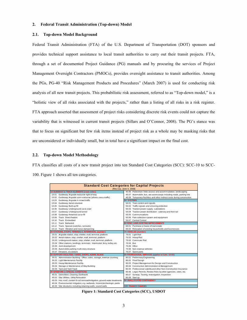
FTA classifies all costs of a new transit project into ten Standard Cost Categories (SCC): SCC-10 to SCC-
100. Figure 1 shows all ten categories.
Figure 1: Standard Cost Categories (SCC), USDOT
10 GUIDEWAY & TRACK ELEMENTS (route miles) 40.06 Pedestrian / bike access and accommodation, landscaping
10.01 Guideway: At-grade exclusive right-of-way 40.07 Automobile, bus, van accessways including roads, parking lots
10.02 Guideway: At-grade semi-exclusive (allows cross-traffic) 40.08 Temporary Facilities and other indirect costs during construction
10.03 Guideway: At-grade in mixed traffic 50 SYSTEMS10.04 Guideway: Aerial structure 50.01 Train control and signals
10.05 Guideway: Built-up fill 50.02 Traffic signals and crossing protection
10.06 Guideway: Underground cut & cover 50.03 Traction power supply: substations
10.07 Guideway: Underground tunnel 50.04 Traction power distribution: catenary and third rail
10.08 Guideway: Retained cut or fill 50.05 Communications
10.09 Track: Direct fixation 50.06 Fare collection system and equipment
10.10 Track: Embedded 50.07 Central Control
10.11 Track: Ballasted
10.12 Track: Special (switches, turnouts) 60.01 Purchase or lease of real estate
10.13 Track: Vibration and noise dampening 60.02 Relocation of existing households and businesses
20 STATIONS, STOPS, TERMINALS, INTERMODAL (number) 70 VEHICLES (number)20.01 At-grade station, stop, shelter, mall, terminal, platform 70.01 Light Rail
20.02 Aerial station, stop, shelter, mall, terminal, platform 70.02 Heavy Rail
20.03 Underground station, stop, shelter, mall, terminal, platform 70.03 Commuter Rail
20.04 Other stations, landings, terminals: Intermodal, ferry, trolley, etc. 70.04 Bus
20.05 Joint development 70.05 Other
20.06 Automobile parking multi-story structure 70.06 Non-revenue vehicles
20.07 Elevators, escalators 70.07 Spare parts
30 SUPPORT FACILITIES: YARDS, SHOPS, ADMIN. BLDGS30.01 Administration Building: Office, sales, storage, revenue counting 80.01 Preliminary Engineering
30.02 Light Maintenance Facility 80.02 Final Design
30.03 Heavy Maintenance Facility 80.03 Project Management for Design and Construction
30.04 Storage or Maintenance of Way Building 80.04 Construction Administration & Management
30.05 Yard and Yard Track 80.05 Professional Liability and other Non-Construction Insurance
40 SITEWORK & SPECIAL CONDITIONS 80.06 Legal; Permits; Review Fees by other agencies, cities, etc.
40.01 Demolition, Clearing, Earthwork 80.07 Surveys, Testing, Investigation, Inspection
40.02 Site Utilities, Utility Relocation 80.08 Start up
40.03 Haz. mat'l, contam'd soil removal/mitigation, ground water treatments 90 UNALLOCATED CONTINGENCY40.04 Environmental mitigation, e.g. wetlands, historic/archeologic, parks
40.05 Site structures including retaining walls, sound walls 100 FINANCE CHARGES
Standard Cost Categories for Capital Projects(Rev.11a, June 4, 2008)
60 ROW, LAND, EXISTING IMPROVEMENTS
80 PROFESSIONAL SERVICES (applies to Cats. 10-50)
4
Costs in SCC 90, Unallocated Contingency, and SCC 100, Financial Charges, are not considered in the Top-
down procedure. The remaining categories should be carefully reviewed to identify all allocated
contingencies. Then, these contingencies are removed from the estimate to arrive at the Base Cost Estimate
(BCE) in each category (Sillars and O’Connor, 2008). Using Top-down model, the overall necessary
contingency budget with respect to different confidence levels is determined. The approach assumes that
each cost category follows a lognormal distribution that can be identified by estimating the 10th and 90th
percentile values of each cost component. The BCE is usually considered to be the 10th percentile of the
lognormal distribution. The 90th percentile of the distribution is estimated from Eq. (1):
90 10 (1)
β is dependent on the level of risk in project delivery stages and ranges from 1.0 to 2.5 and above. A β value
of 1.0 means that there is no risk associated with the BCE. The more the project progresses, the smaller the
value of β. Using the 10th and 90th percentile of each cost component, and using Lognormal Distribution
equations, the mean and standard deviation of each cost component are calculated (Eqs. (2)-(7)). In these
equations, μ and σ are parameters of the underlying normal distribution; ∅ denotes the standard normal
distribution and ∅ represents the inverse of cumulative function for the standard normal distribution; the
mean and variance of the lognormal distribution are given in Eqs. (6) and (7).
% 10 (2)
% 90 (3)
ln ∅ ∅ (4)
ln ∅ ∅ (5)
⁄ (6)
1 (7)
The sum of these cost components that represents the total cost is calculated using the Central Limit
Theorem and assumes normality for the sum of lognormal components. To form the cumulative distribution,
the model first assumes that all cost categories are completely correlated, 1.0, and then assumes that
5
there is no correlation, 0. This procedure produces two cumulative distributions for total cost. Note that
the assumption of normality is not correct when components are fully correlated. Indeed, it can be proven
that the total will follow a lognormal distribution. However, this is what the top-down approach assumes. A
“First Order Approximation” distribution, which is the final product of the proposed top-down approach, is
created by finding the one-third point of the total difference in variance between the two aforementioned
distributions. This process is applied to project cost components, and several scenarios are run at the
beginning of various project phases.
2.3. How to Assign β Values to Different SCCs at the Various Project Delivery Stages
Based on the historical data and lessons learned from previous transit projects, a set of recommended β
values is suggested by PG-40. It is a risk analyst’s responsibility to find the most appropriate β factors to
assign to each SCC by considering the unique and specific characteristics of every project:
1. Requirement risks: those associated with the definition of basic project needs and transit system
requirements to meet those needs (β ≥2.5);
2. Design risks: those involved with the engineering design of the transit system (2.5> β ≥2.0);
3. Market risks: those associated with the procurement of construction services and other system
components (2.0> β ≥1.75);
4. Construction risks: those associated with the actual construction of the systems (1.75> β ≥1.05).
The guidelines provide specific β values to be applied to various Standard Cost Categories (SCC) for the
transit project. The values of β may vary throughout project implementation at each key stage of project
development. These recommendations will be used in the next section to assign the β’s at three different
stages of the project completion.
2.4. Applying the Top-down Model to U.S. Data
The value of β will vary from project to project and depend on the level of project development. As the
project design progresses, the values of β tend to decrease. However, one can estimate an average β for the
average transit project in the United States. The objective here is to calculate the average range for U.S.
6
transit projects costs using the guidelines provided in PG-40. To this end, 51 transit projects in the U.S. (30
heavy rail and 21 light rail) for which actual costs were reported (Booz Allen Hamilton, 2003 and 2004)
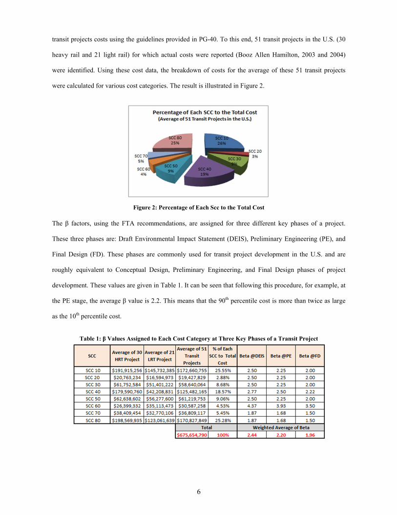
were identified. Using these cost data, the breakdown of costs for the average of these 51 transit projects
were calculated for various cost categories. The result is illustrated in Figure 2.
Figure 2: Percentage of Each Scc to the Total Cost
The β factors, using the FTA recommendations, are assigned for three different key phases of a project.
These three phases are: Draft Environmental Impact Statement (DEIS), Preliminary Engineering (PE), and
Final Design (FD). These phases are commonly used for transit project development in the U.S. and are
roughly equivalent to Conceptual Design, Preliminary Engineering, and Final Design phases of project
development. These values are given in Table 1. It can be seen that following this procedure, for example, at
the PE stage, the average β value is 2.2. This means that the 90th percentile cost is more than twice as large
as the 10th percentile cost.
Table 1: β Values Assigned to Each Cost Category at Three Key Phases of a Transit Project
7
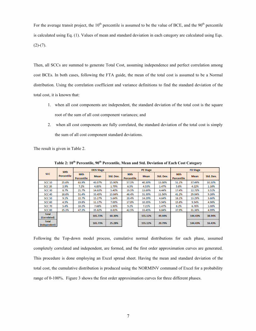
For the average transit project, the 10th percentile is assumed to be the value of BCE, and the 90th percentile
is calculated using Eq. (1). Values of mean and standard deviation in each category are calculated using Eqs.
(2)-(7).
Then, all SCCs are summed to generate Total Cost, assuming independence and perfect correlation among
cost BCEs. In both cases, following the FTA guide, the mean of the total cost is assumed to be a Normal
distribution. Using the correlation coefficient and variance definitions to find the standard deviation of the
total cost, it is known that:
1. when all cost components are independent, the standard deviation of the total cost is the square
root of the sum of all cost component variances; and
2. when all cost components are fully correlated, the standard deviation of the total cost is simply
the sum of all cost component standard deviations.
The result is given in Table 2.
Table 2: 10th Percentile, 90th Percentile, Mean and Std. Deviation of Each Cost Category
Following the Top-down model process, cumulative normal distributions for each phase, assumed
completely correlated and independent, are formed, and the first order approximation curves are generated.
This procedure is done employing an Excel spread sheet. Having the mean and standard deviation of the
total cost, the cumulative distribution is produced using the NORMINV command of Excel for a probability
range of 0-100%. Figure 3 shows the first order approximation curves for three different phases.
8
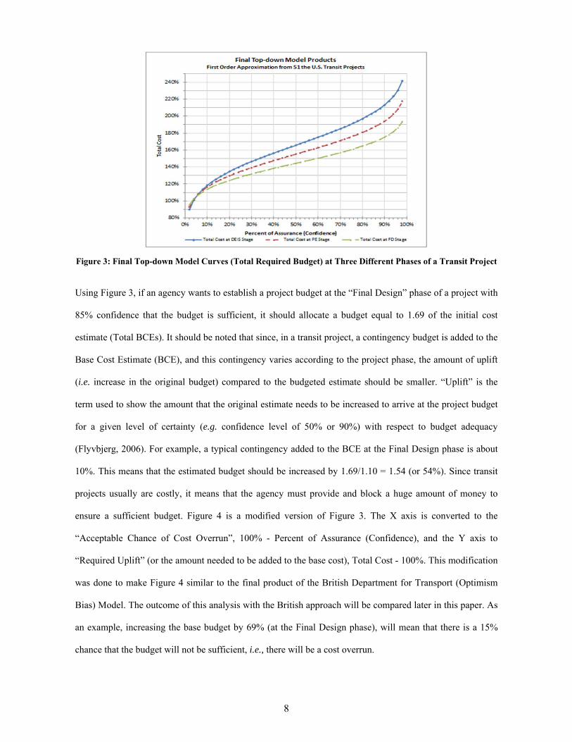
Figure 3: Final Top-down Model Curves (Total Required Budget) at Three Different Phases of a Transit Project
Using Figure 3, if an agency wants to establish a project budget at the “Final Design” phase of a project with
85% confidence that the budget is sufficient, it should allocate a budget equal to 1.69 of the initial cost
estimate (Total BCEs). It should be noted that since, in a transit project, a contingency budget is added to the
Base Cost Estimate (BCE), and this contingency varies according to the project phase, the amount of uplift
(i.e. increase in the original budget) compared to the budgeted estimate should be smaller. “Uplift” is the
term used to show the amount that the original estimate needs to be increased to arrive at the project budget
for a given level of certainty (e.g. confidence level of 50% or 90%) with respect to budget adequacy
(Flyvbjerg, 2006). For example, a typical contingency added to the BCE at the Final Design phase is about
10%. This means that the estimated budget should be increased by 1.69/1.10 = 1.54 (or 54%). Since transit
projects usually are costly, it means that the agency must provide and block a huge amount of money to
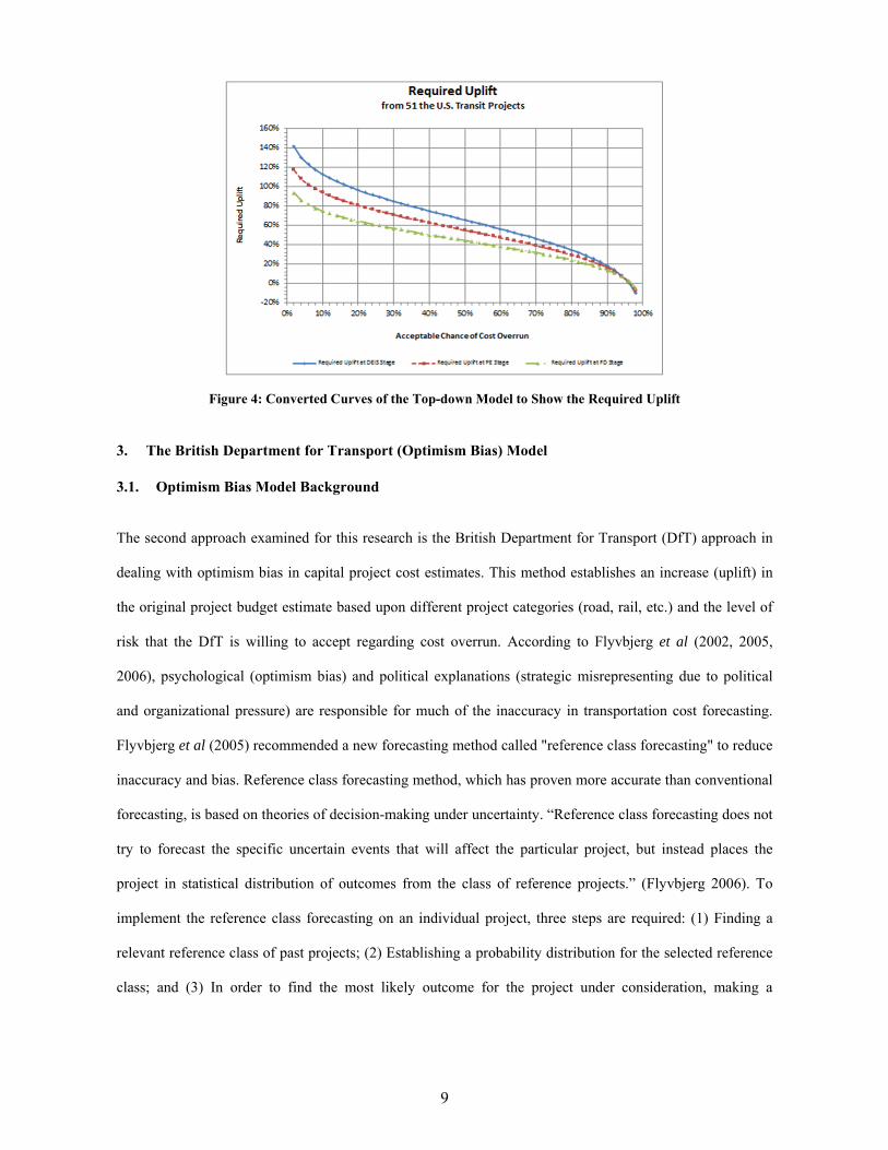
ensure a sufficient budget. Figure 4 is a modified version of Figure 3. The X axis is converted to the
“Acceptable Chance of Cost Overrun”, 100% - Percent of Assurance (Confidence), and the Y axis to
“Required Uplift” (or the amount needed to be added to the base cost), Total Cost - 100%. This modification
was done to make Figure 4 similar to the final product of the British Department for Transport (Optimism
Bias) Model. The outcome of this analysis with the British approach will be compared later in this paper. As
an example, increasing the base budget by 69% (at the Final Design phase), will mean that there is a 15%
chance that the budget will not be sufficient, i.e., there will be a cost overrun.
9
Figure 4: Converted Curves of the Top-down Model to Show the Required Uplift
3. The British Department for Transport (Optimism Bias) Model
3.1. Optimism Bias Model Background
The second approach examined for this research is the British Department for Transport (DfT) approach in
dealing with optimism bias in capital project cost estimates. This method establishes an increase (uplift) in
the original project budget estimate based upon different project categories (road, rail, etc.) and the level of
risk that the DfT is willing to accept regarding cost overrun. According to Flyvbjerg et al (2002, 2005,
2006), psychological (optimism bias) and political explanations (strategic misrepresenting due to political
and organizational pressure) are responsible for much of the inaccuracy in transportation cost forecasting.
Flyvbjerg et al (2005) recommended a new forecasting method called "reference class forecasting" to reduce
inaccuracy and bias. Reference class forecasting method, which has proven more accurate than conventional
forecasting, is based on theories of decision-making under uncertainty. “Reference class forecasting does not
try to forecast the specific uncertain events that will affect the particular project, but instead places the
project in statistical distribution of outcomes from the class of reference projects.” (Flyvbjerg 2006). To
implement the reference class forecasting on an individual project, three steps are required: (1) Finding a
relevant reference class of past projects; (2) Establishing a probability distribution for the selected reference
class; and (3) In order to find the most likely outcome for the project under consideration, making a
10
comparison between the project under consideration and the reference class distribution (Flyvbjerg et al,
2005).
According to Supplementary Green Book (2003): “There is a demonstrated, systematic tendency for project
appraisers to be overly optimistic. To redress this tendency, appraisers should make explicit, empirically
based adjustments to the estimates of a project’s costs, benefits, and duration… It is recommended that these
adjustments be based on data from past projects or similar projects elsewhere.” To this end, in 2004, the
British Department for Transport and HM Treasury published a guide, “Procedures for dealing with
Optimism Bias in Transport Planning,” based on the work conducted by Flyvbjerg and COWI (The British
DfT, 2004). It establishes a guide for selected reference classes of transport infrastructure projects to prevent
cost overrun. This approach is hereafter called the “Optimism Bias Model” method in this paper.
3.2. The Optimism Bias Model Methodology
In the DfT guide, transportation projects have been divided into a number of distinct groups. These groups
include road, rail, fixed links, buildings, and IT projects and have been selected in order to have statistically
similar risk of cost overrun based on the study of an international database of 258 transportation projects. In
this paper, the focus is only on rail projects, as the analyzed transit projects for the US case were almost
exclusively rail projects.
In the DfT guide, cost overrun is defined as the difference between the actual cost (final cost) and the
estimated cost, which is the forecasted cost at the time of approval of/decision to build a project, in
percentage of estimated cost. Where the approval point is not clear in the project planning process, the
closest available estimate is used. For each category, the probability distribution for cost overrun as the share
of projects with a given maximum cost overrun was created. Having established the empirical cumulative
distribution, uplifts are set up as a function of the level of risk that the DfT is willing to accept regarding cost
overrun. If the DfT wants to accept a higher risk, then a lower uplift is required. The readers are referred to
the British DfT (2004) and Flyvbjerg (2006) for a thorough description of the Optimism Bias methodology.
11
3.3. Applying the Optimism Bias Model to U.S. Data
To generate a reference class, 22 rail projects across the U.S. were selected. To reach the objective of this
paper, the Optimism Bias Model approach is first applied to these projects. Then the results are compared
with the results of applying the USDOT approach to the same data. These projects were part of a study
conducted by Booz Allen Hamilton (2005). As part of this research effort, cost overruns for 22 major rail
projects were calculated by considering estimated budgets at various stages of these projects. For each
project, the cost overrun/underrun was calculated at the DEIS, PE, and FD stages by comparing these
estimates with the actual cost of projects. Although, DfT calculates the cost overrun relative to the estimate
at the point of approval of/decision to build, in order to compare FTA and DfT models, cost overrun has
been calculated at the DEIS, PE, and FD stages. PE can be considered equivalent to the British agencies’
preparation of their initial budgets. In this way, these two models can be compared. It should be noted that
the main criteria in selecting these 22 projects for inclusion in the original study was the availability of data.
In other words, the author was not trying to identify and select projects that were notorious for cost overrun
or delay.
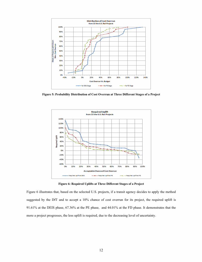
In order to find the probability distribution for each stage, the cost overruns/underruns of 22 projects were
sorted in ascending order. Then, for each cost overrun/underrun, the correspondent probability was
calculated by dividing the number of projects having the cost overrun less than that by 22. Figure 5 depicts
the probability distributions for the DEIS, PE, and FD stages. For instance, Figure 5 shows that at the DEIS
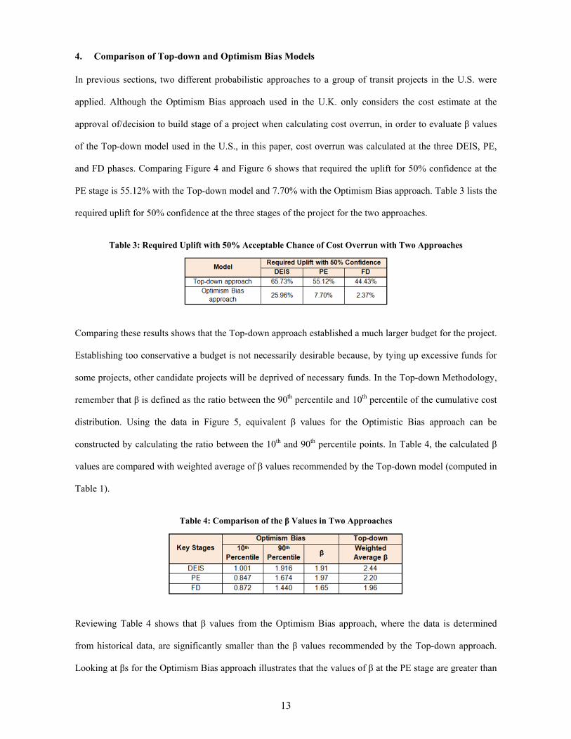
stage, 60% of projects have the maximum cost overrun of 23%. Then the required uplift curve is calculated
(Figure 6).
12
Figure 5: Probability Distribution of Cost Overrun at Three Different Stages of a Project
Figure 6: Required Uplifts at Three Different Stages of a Project
Figure 6 illustrates that, based on the selected U.S. projects, if a transit agency decides to apply the method
suggested by the DfT and to accept a 10% chance of cost overrun for its project, the required uplift is
91.61% at the DEIS phase, 67.36% at the PE phase, and 44.01% at the FD phase. It demonstrates that the
more a project progresses, the less uplift is required, due to the decreasing level of uncertainty.
13
4. Comparison of Top-down and Optimism Bias Models
In previous sections, two different probabilistic approaches to a group of transit projects in the U.S. were
applied. Although the Optimism Bias approach used in the U.K. only considers the cost estimate at the
approval of/decision to build stage of a project when calculating cost overrun, in order to evaluate β values
of the Top-down model used in the U.S., in this paper, cost overrun was calculated at the three DEIS, PE,
and FD phases. Comparing Figure 4 and Figure 6 shows that required the uplift for 50% confidence at the
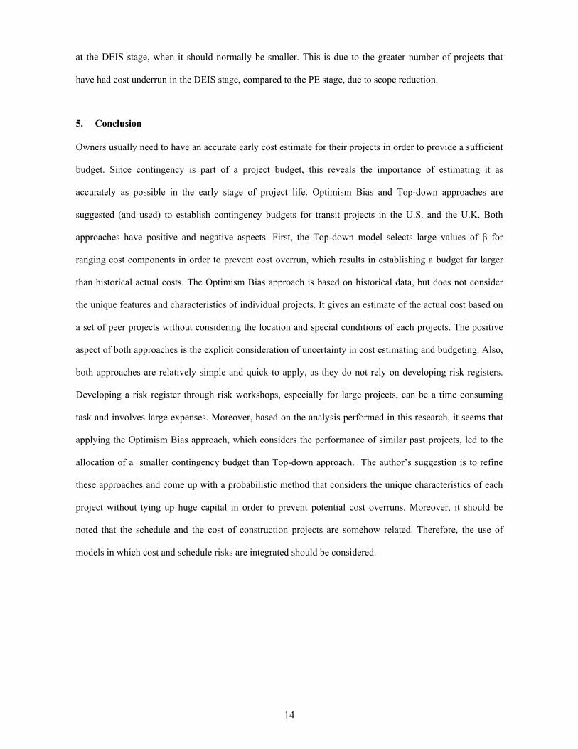
PE stage is 55.12% with the Top-down model and 7.70% with the Optimism Bias approach. Table 3 lists the
required uplift for 50% confidence at the three stages of the project for the two approaches.
Table 3: Required Uplift with 50% Acceptable Chance of Cost Overrun with Two Approaches
Comparing these results shows that the Top-down approach established a much larger budget for the project.
Establishing too conservative a budget is not necessarily desirable because, by tying up excessive funds for
some projects, other candidate projects will be deprived of necessary funds. In the Top-down Methodology,
remember that β is defined as the ratio between the 90th percentile and 10th percentile of the cumulative cost
distribution. Using the data in Figure 5, equivalent β values for the Optimistic Bias approach can be
constructed by calculating the ratio between the 10th and 90th percentile points. In Table 4, the calculated β
values are compared with weighted average of β values recommended by the Top-down model (computed in
Table 1).
Table 4: Comparison of the β Values in Two Approaches
Reviewing Table 4 shows that β values from the Optimism Bias approach, where the data is determined
from historical data, are significantly smaller than the β values recommended by the Top-down approach.
Looking at βs for the Optimism Bias approach illustrates that the values of β at the PE stage are greater than
14
at the DEIS stage, when it should normally be smaller. This is due to the greater number of projects that
have had cost underrun in the DEIS stage, compared to the PE stage, due to scope reduction.
5. Conclusion
Owners usually need to have an accurate early cost estimate for their projects in order to provide a sufficient
budget. Since contingency is part of a project budget, this reveals the importance of estimating it as
accurately as possible in the early stage of project life. Optimism Bias and Top-down approaches are
suggested (and used) to establish contingency budgets for transit projects in the U.S. and the U.K. Both
approaches have positive and negative aspects. First, the Top-down model selects large values of β for
ranging cost components in order to prevent cost overrun, which results in establishing a budget far larger
than historical actual costs. The Optimism Bias approach is based on historical data, but does not consider
the unique features and characteristics of individual projects. It gives an estimate of the actual cost based on
a set of peer projects without considering the location and special conditions of each projects. The positive
aspect of both approaches is the explicit consideration of uncertainty in cost estimating and budgeting. Also,
both approaches are relatively simple and quick to apply, as they do not rely on developing risk registers.
Developing a risk register through risk workshops, especially for large projects, can be a time consuming
task and involves large expenses. Moreover, based on the analysis performed in this research, it seems that
applying the Optimism Bias approach, which considers the performance of similar past projects, led to the
allocation of a smaller contingency budget than Top-down approach. The author’s suggestion is to refine
these approaches and come up with a probabilistic method that considers the unique characteristics of each
project without tying up huge capital in order to prevent potential cost overruns. Moreover, it should be
noted that the schedule and the cost of construction projects are somehow related. Therefore, the use of
models in which cost and schedule risks are integrated should be considered.
15
6. References
Booz Allen Hamilton (Schneck, D. and Laver, R.). (2003). “Light Rail Transit Capital Cost Study
Update.” Federal Transit Administration, Washington, D.C.
Booz Allen Hamilton (Schneck, D. and Laver, R.). (2004). “Heavy Rail Transit Capital Cost Study
Update.” Federal Transit Administration, Washington, D.C.
Booz Allen Hamilton (2005). “Final Report: Managing Capital Costs of Major Federally Funded
Public Transportation Projects”, Project G-07, Transit Cooperation Research Program.
(TCRP), McLean, VA, November.
Federal Transit Administration. (2007). “Risk Management Products and Procedures”, PG# 40, March 29.
Federal Transit Administration. (2003). “Risk Assessment and Mitigation Procedures”, PG# 22, December
8.
Flyvbjerg, B. (2006). “From Nobel Prize to Project Management: Getting Risk Right”, Project Management
Journal, August, pp. 5-15.
Flyvbjerg, B. (2005). “Design by Deception: The Politics of Megaprojects Approval”, Harvard
Design Magazine, Spring/Summer, pp. 50-59.
Flyvbjerg, B., Holm, M. K. S., and Buhl, S. L. (2005). “How (In)accurate Are Demand Forecasts in
Public Works Projects?”, Journal of the American Planning Association, Vol. 71, No. 2,
Spring, pp. 131-146.
Flyvbjerg, B., Holm, M. K. S., and Buhl, S. L. (2002). “Underestimating Costs in Public Works
Projects: Error or Lie?”, Journal of the American Planning Association, Vol. 68, No.3,
Summer, pp. 279-295.
HM Treasury of the U.K. (2003). Supplementary Green Book Guidance: Optimism Bias, London,
U.K.
Sillars, D. and O’Connor, M. (2008). “Risk-Informed Project Oversight at the FTA”, TRB 2008
Annual Meeting.
The British Department for Transport. (2004). “Procedure for Dealing with Optimism Bias in
Transport Planning”, Guidance Document, June.