Evaluation of cloud based approaches to data quality ...

1

Aalto University

School of Science

Master’s Programme in Service Design and Engineering

Aftab Ansari

Evaluation of cloud based approaches to data

quality management

Master’s Thesis

Espoo, January 25, 2016

Supervisor: Professor Jukka K. Nurminen, Aalto University

Instructor: Seamus Moloney, M.Sc. (Tech.)

2

Aalto University

School of Science

Degree Programme in Computer Science and Engineering

Master’s Programme in Service Design and Engineering

ABSTRACT OF THE MASTER’S THESIS

Author: Aftab Ansari

Title: Evaluation of cloud based approaches to data quality management

Number of pages:83 Date:25/01/2016 Language: English

Professorship: Computer Sciences Code: T-106

Supervisor: Prof. Jukka K. Nurminen

Advisor: Seamus Moloney, M.Sc. (Tech.)

Abstract: Quality of data is critical for making data driven business decisions. Enhancing the quality of data

enables companies to make better decisions and prevent business losses. Systems similar to Extract

Transform and Load (ETL) are often used to clean and improve the quality of data. Currently, businesses

tend to collect a massive amount of customer data, store it in the cloud, and analyze the data to gain statistical

inferences about their products, services, and customers. Cheaper storage, constantly improving approaches

to data privacy and security provided by cloud vendors, such as Microsoft Azure, Amazon Web Service,

seem to be the key driving forces behind this process.

This thesis implements Azure Data Factory based ETL system that serves the purpose of data quality

management in the Microsoft Azure Cloud platform. In addition to Azure Data Factory, there are four other

key components in the system: (1) Azure Storage for storing raw, and semi cleaned data; (2) HDInsight for

processing raw and semi cleaned data using Hadoop clusters and Hive queries; (3) Azure ML Studio for

processing raw and semi cleaned data using R scripts and other machine learning algorithms; (4) Azure SQL

database for storing the cleaned data. This thesis shows that using Azure Data factory as the core component

offers many benefits because it helps in scheduling jobs, and monitoring the whole data transformation

processes. Thus, it makes data intake process more timely, guarantees data reliability, simplifies data

auditing. The developed system was tested and validated using sample raw data.

Keywords: Data quality management, ETL, Data cleaning, Hive, Hadoop, Azure Microsoft

3

Acknowledgements

I would like to thank my supervisor for this thesis professor Jukka Nurminen and the

instructor, Seamus Moloney, for their valuable comments and guidance on various draft

versions of this thesis work. I would also like to thank Antti Pirjeta for providing his

comments on R scripting and other data analysis part. Also, I would like to thank Tommi

Vilkamo, Jakko Teinila, and Tanja Vuoksima for taking time to discuss different phases of

the work and giving their valuable feedbacks. Finally, I would like to thank the case company

for proving me opportunity for doing my thesis and giving me access to the raw data and

MSDN subscription for accessing different tools and services available on Microsoft Azure.

Espoo, January 25, 2016

Aftab Ansari

4

Abbreviations and Acronyms

ADF Azure Data Factory

API Application Program Interface

AWS Amazon Web Service

Amazon EC2 Amazon Elastic Compute Cloud

Amazon EMR Amazon Elastic MapReduce

Amazon RDS Amazon Relational Database Service

Amazon S3 Amazon Simple Storage Service

CI Confidence Interval

ETL Extract Transform and Load

EWD Enterprise Data Warehouse

FTP File Transfer Protocol

HDFS Hadoop Distributed File System

IDE Integrated Development Environment

JSON JavaScript Object Notation

MSDN Microsoft Developer Network

MS SQL Microsoft Structured Query Language

RDBMS Relational Database Management System

SDK Software Development Kits

SaaS Software as Service

SQL Structured Query Language

WASB Windows Azure Storage Blob

5

Contents

Introduction .......................................................................................................................... 7

1.1 Research goals .............................................................................................................. 9

1.2 Research questions ...................................................................................................... 10

1.3 Structure of this thesis ................................................................................................. 11

Background ......................................................................................................................... 12

2.1 Architectural background ...................................................................................... 12

2.1.1 Related work to data quality management ............................................................... 14

2.1.2 CARAT .................................................................................................................... 18

2.1.3 CloudETL ................................................................................................................ 19

2.2 Data quality management ...................................................................................... 20

2.2.1 Advantages of cloud technologies in data quality management .............................. 21

2.2.2 Azure Data Factory (ADF) ...................................................................................... 22

2.2.3 Data Pipeline ........................................................................................................ 24

Implemented Data Factory for data quality management ............................................. 28

3.1 Creating ADF .............................................................................................................. 29

3.1.1 Windows Azure Storage....................................................................................... 30

3.1.2 Azure HDInsight .................................................................................................. 31

3.1.3 Azure ML Studio .................................................................................................. 33

3.1.4 Azure SQL Database ............................................................................................ 37

3.2 Proposed Architecture ................................................................................................. 37

3.3 Deployment of the data quality management system ................................................. 39

Tested sample data ............................................................................................................. 46

6

4.1 Sample data source ..................................................................................................... 46

4.2 Known issues in sample data ...................................................................................... 48

4.3 Data quality problems and data cleaning rule definitions ........................................... 54

4.4 Assessment of data cleaning rules .............................................................................. 55

Results and Evaluations ..................................................................................................... 56

5.1 Defining criteria to identify false positive .................................................................. 60

5.2 Confidence Interval (CI) ............................................................................................. 61

5.3 Minimizing false positive ........................................................................................... 66

5.4 Scalability and performance of the ETL ..................................................................... 66

5.5 Pricing ......................................................................................................................... 71

Discussions ........................................................................................................................... 73

6.1 Complexity of development and usage ....................................................................... 73

6.2 Use cases ..................................................................................................................... 73

6.3 Learning outcomes ...................................................................................................... 74

6.4 Strengths and weaknesses of the ADF ........................................................................ 75

Conclusions ......................................................................................................................... 76

CHAPTER 1. INTRODUCTION

7

Chapter 1

Introduction

In recent years, collecting and analyzing feedback from end users has become one of most

important tasks for many companies who aim to improve the quality of their products or

services. Regardless of being startups or corporate giants, end user feedback is crucial; hence,

managing such feedback data is as significant as managing products. To increase

productivity, organizations must manage information as they manage products (Wang 1998).

However, it is not always easy to manage information in a large scale. The amount of end

user feedback on daily basis has dramatically increased due to substantial growth in digital

data. This has taken the form of big-data scenario. Big Data refers to a great volume of data

that is unsuitable for typical relational databases treatment (Garlassu 2013; Fisher et al. 2012;

Lohr 2012; Madden 2012). The colossal volume of data generated by the users contain

valuable information that a company can utilize to understand how their products or services

are performing with end users’ perspective. However, processing such a massive amount of

data to gain valuable insight is a major challenge. As the volume of the big data increases, it

also increases the complexity and relationships between the underlying data and hence

requires high-performance computing platforms to process and gain valuable insights (Wu

2014; Labrinidis & Jagadish 2012).

High quality data is data that is useful, usable, and hence fit for use by data consumers (Strong

et al 1997). Currently, most information systems operate as networks, which significantly

increases the set of potential data sources. On one hand, the increased number of data sources

provides an opportunity to select and compare data from a broader range of data sources to

detect and correct errors for improving the overall quality of data. However, this increased

number of data sources also adds complexity in maintaining the overall data quality (Batini

et al 2009; Haug 2013; Zhang et al 2003.) When a company makes decisions based on the

available data, the quality of data is a highly important factor. Poor quality data, also known


8

as dirty data, can cause deleterious impact on the overall health of company (Eckerson 2002).

Data is rarely 100% accurate but it can be improved by data cleaning.

Extract, Transform, and Load (henceforth ETL) is a typical process of handling data cleaning

in the enterprise world where data is extracted in multiple formats and from multiple sources.

ETL can be seen as a collection of tools that play a significant role in collection and discovery

of data quality issues, and efficiently loading large volumes of data into a data warehouse

(Chaudhuri et al 2011; Agarwal et al 2008.) One of the key purposes of a data warehouse is

to enable systematic or ad-hoc data mining (Stonebraker 2002). ETL and data cleaning tools

constitute a major expenditure in a data warehouse project. A data warehouse project mainly

consists of two categories of expenditure: 1) one-time costs, such as hardware, software, disk,

CPU, DBMS, network, and terminal analysis, and 2) recurring costs, including hardware

maintenance, software maintenance, ongoing refreshment, integration transformation

maintenance, and data model maintenance. (Bill 1997). However, ETL and data cleaning

tools which constitute costs from both categories are estimated to account for at least one

third of budget, and this number can rise up to 80%. The ETL process alone usually amounts

to about 55% of the total costs of data warehouse runtime (Vassiliadis et al 2002). As such

ETL is highly expensive and still includes several challenges.

To point out some key challenges and work around the ETL, Chaudhary et al. (2011) states

that several data structures, optimizations, and query processing techniques have been

developed over the past two decades to execute complex SQL queries, such as ad hoc queries

over large volume of data. However, with accelerating growth of data, the challenges of

processing data is only growing. As implied by Vassiliadis et al. (2002), it is clear that the

right architecture and efficiency in data cleaning can bring notable value for both data

warehouses and enterprises spending heavy budgets on data cleaning. Although ETL appears

to be the dominating method of data cleaning for data quality management, there has been a

number of challenges when applying ETL process to a large volume of data, which has led

data scientists to find workarounds and build custom architecture for ETL process. However,

with the rapid growth of data forms, volume, and velocity, the traditional ETL process that

requires a proprietary data warehouse has become less relevant and not sufficiently powerful


9

for managing quality of Big Data. Currently, cloud-based ETL is an emerging trend mainly

due to its high scalability, low cost, and convenience in development and deployment. This

thesis aims to leverage tools and services offered by cloud providers and build a cloud based

ETL system for managing the quality of data.

1.1 Research goals

This thesis has three aims: background study, propose architecture, and implementation. The

main objective of this thesis is to build a cloud based ETL system for data quality

management. To achieve this objective, this thesis evaluates an existing cloud based

approach similar to ETL for managing data quality and then proposes a new, efficient and

scalable architecture. The new architecture can also harness the strength of machine learning

in data quality management.

To understand better the practical implications of this cloud based approach, a sample

telemetry data provided by the client company is processed aiming to improve its quality.

The efficiency and scalability of data quality management is evaluated based on the obtained

results. The proposed architecture is compared against other similar data quality management

systems' architecture to ensure the validity. When processing the sample data (which contains

dirty data), false positives are identified and minimized to ensure better conclusions. Dirty

data can lead to the wrong conclusions being made, which is often classified as a false

positive. For example, if data suggests that the average battery life of a mobile device is x

hours when it is not, that is a false positive. In data cleaning, statistical rules can be applied

to detect and remove incorrect data in order to minimize false positives. This uses statistical

methods to investigate how false positives can be minimized and how the confidence interval

can be quantified for the sample data. This thesis proposes that a key component of the data

quality management system is data pipelines. Data pipeline features of the Amazon and

Azure platforms are also compared in order to determine the key differences.


10

1.2 Research questions

This thesis aims to determine strategies for ensuring data quality management using the latest

and most efficient cloud based technologies and approaches. The thesis focuses on the

following four research questions.

RQ1: What is the most suitable architecture for data quality management in the

cloud?

Chapter 3 presents alternative cloud based tools for data quality management. With the

evaluated tools, an architecture is designed and proposed which aims to satisfy requirement

of improved data quality management. The proposed architecture is compared against the

architecture of a research project named “CARAT” and “CloudETL”.

RQ2: How to minimize false positives when applying automatic data cleaning?

Chapter 5 discusses the process of minimizing false positives in automatic data cleaning in

detail. First data cleaning is performed on a sample telemetry dataset by using the proposed

architecture of this thesis. Section 3.2 discusses about the proposed architecture in detail.

Data cleaning rules are defined using Hive scripts to detect and remove incorrect data and

minimize the false positives. To perform automatic data cleaning, this thesis uses cloud based

Hadoop clusters offered by Microsoft Azure’s HDInsight, which supports Hive query and

can be run on demand. A monitoring mechanism for applied data cleaning rules is developed

to visualize the performance and progress of the applied cleaning rules. Microsoft’s Azure

Data Factory (ADF) provides monitoring mechanism for data cleaning rules.

RQ3: How to quantify confidence interval for the false positive rate?

Chapter 5 presents the details of the process of quantifying confidence interval for the false

positive rate of the data cleaning rules. A confidence interval of 95% is calculated for each

false positive rate of cleaning rules using the binomial distribution. An R-script is used to

calculate 95% confidence interval.

RQ4: What are the advantages of using cloud technologies instead of creating

custom data cleaning rules?


11

Chapter 2 discusses various advantages of using cloud technologies in the context of data

cleaning. This thesis also investigates the key advantages of cloud technologies based on

various literature.

1.3 Structure of this thesis

This thesis is organized as follows. Chapter 2 presents a background study about data quality

management. It highlights the importance of data cleaning in the current context of increasing

volume, velocity, and diversity of data. Two related projects and their architectures are

studied briefly in this chapter. Chapter 3 describes in detail the description of the

implemented Azure Data Factory. The architecture in general and its key components are

described. Some example code snippets are presented to demonstrate how other tools and

technologies on Azure platform can be integrated with Azure Data Factory. Chapter 4

describes briefly the sample data processed using the Azure Data Factory. This chapter also

discusses the identified data quality problems in the sample data, selection and assessment

of data cleaning rules. Chapter 5 discusses the results of the sample data cleaning over the

implemented Azure Data Factory. Chapter 6 concludes the thesis and presents suggestions

for future development.

CHAPTER 2. BACKGROUND

12

Chapter 2

Background

This thesis presents background studies with two main perspectives: (1) architectural

background which studies cloud based architectures implemented for data quality

management and discusses examples of related work, (2) data quality management which

studies about the challenges of data quality management. Data cleaning in particular is

studied as a technique to improve the quality of data. Moreover, the advantages of using

cloud technologies for managing quality of data is discussed.

2.1 Architectural background

Chaudhuri et al. (2011) argues that since more data is generated as digital data, there is an

increasing desire to build low-cost data platforms that can support much larger data volume

than that traditionally handled by relational database management systems (RDBMSs).

Figure 1 shows typical architecture of handling data for business intelligence in the enterprise

environment.

Figure 1. Typical business intelligence architecture (Chaudhuri 2011, p. 90)


13

As can be seen from Figure 1, data can come from multiple sources. These sources can be

operational databases across departments within the organization, and external vendors. As

these different sources contain data in different formats, and volume, there are

inconsistencies and data quality issues to deal with when integrating, cleaning, and

standardizing such data for front-end applications (Roberts et al. 1997; Vijayshankar &

Hellerstein 2001). Moreover, traditional ETL process architectures do not seem to be a good

fit for solving Big Data challenges as currently digital data is growing rapidly and the

architecture for data integration needs to support high scalability. This is mainly because

cloud providers offer highly scalable data storage, and data processing tools and services

which makes it easy to store, integrate, process, and manage data. In addition, services

offered by cloud providers cost less than own data warehouse solution due to the economy

of scale.

The cloud is all about unlimited storage and compute resources to process data which come

from diverse sources and are of big volume, and velocity (Maturana et al. 2014). Data

collection has become a ubiquitous function of large organizations for both record keeping

and supporting variety of data analysis tasks to drive decision making process (Hellerstein

2008; Thusoo et al. 2010). Leveraging data available to business is essential for organizations

and there is a critical need for processing data across geographic locations, on-premises, and

cloud with a variety of data types and volume. The current explosion of data form, size, and

velocity is a clear evidence of the need for one solution to address today's diverse data

processing landscape (Microsoft Azure 2014; Boyd & Kate 2012). Despite the importance

of data collection and analysis, data quality is a pervasive problem that almost every

organization faces (Hellerstein 2008). Therefore, one of the key requirements of such

solution should be the ability to manage the data quality as data integration from diverse data

source, format only adds complexity in data quality.

Currently, the fundamental difficulties for data scientists in efficiently searching for deep

insights in data are (a) identifying relevant fragments of data from diverse data sources, (b)

data cleaning techniques such as approximate joins across two data sources, (c) progressively


14

sampling results of query, (d) obtaining rich data visualization which often requires system

skills, and algorithmic expertise (Chaudhuri 2012.)

According to Redman (as cited in Redman 1998), issues of data quality can be categorized

in main four categories: (1) Issues associated with data "view”. These are typically the

models of real world data that include relevancy, granularity, and level of detail; (2) Issues

associated with data values such as accuracy, consistency, and completeness; (3) Issues

associated with presentation of data which can be format, and ease of interpretation; (4) Other

Issues which can be associated with privacy, security, and ownership.

2.1.1 Related work to data quality management

Three contributing communities (1) Business analysts, (2) solution architects, and (3)

database experts and statisticians (Sidiq et al 2011) are behind the development of newer

systems for data quality management. MapReduce paradigm (chaudhary 2011; Roshan et al

2013) for data management architecture including Hadoop Distributed File System (HDFS)

(Kelley 2014; Stonebraker et al 2010) is a well-known approach among current solutionists

for Big Data solution providers. To ease the life of programmers who prefer structured query

language (SQL) over MapReduce framework, several SQL like language have been

developed over the years that can work on top of MapReduce. These include Sawzall, Pig

Latin, Hive, and Tenzing (Sakr & Liu 2013). The ETL system implemented as part of this

thesis is built to support Big Data scenario which uses Hadoop and Hive for its data cleaning

process.

Apache Hadoop

Apache Hadoop is a framework for distributed processing of large data sets across clusters

of computers using simple programming models (Apache Org, 2015). It is an open source

implementation of the MapReduce framework. Engines based on MapReduce paradigm

(which was originally built for analyzing web documents and web search query logs) are now


15

being targeted for enterprise analytics (Chaudhuri 2011; Herodotos et al 2011). To serve this

purpose, such engines are being extended to support complex SQL-like queries essential for

traditional enterprise data warehousing scenarios. Dahiphale (2014) explains MapReduce as

a framework developed by Google that can process large datasets in distributed fashion.

Further, pointing out the two main phases of MapReduce framework namely Map phase and

Reduce phase, it provides an abstraction of these two phases. During the Map phase, input

data is split into chunks and distributed among multiple nodes to be processed upon by a user

defined Map function. In Reduce phase, data produced by Map function is aggregated. Below

is an example of doing word count using MapReduce.

Texts to read:

1

2

The Map function reads words one at a time and outputs:

1

2

3

4

5

6

7

8

The shuffle phase between Map and Reduce phase creates a list of values associated with

each key which becomes input for Reduce function.

1

2

3

4

Hello World Bye World

Hello Hadoop Goodbye Hadoop

(Hello, 1)

(World, 1)

(Bye, 1)

(World, 1)

(Hello, 1)

(Hadoop, 1)

(Goodbye, 1)

(Hadoop, 1)

(Bye, (1))

(Goodbye, (1))

(Hadoop, (1, 1))

(Hello, (1, 1))

(World, (1, 1))


16

5

Finally the Reduce function sums the numbers in the list for each key and outputs (word,

count) pairs as given below.

1

2

3

4

5

Jayalath et al. (2014) describes an implementation of MapReduce framework such as Apache

Hadoop as part of standard toolkit for processing large data sets using cloud resources.

Data cleaning and standardizing using cloud technologies seems to be emerging as a

replacement of traditional ETL processes. Some of the key cloud platforms including

Amazon Web Services (AWS), and Microsoft Azure have been offering services such as data

pipelines for data integration, and computing service. These services supports parallel

reading using technologies including MapReduce, Hive, and Pig running in settings such as

Hadoop.

Apache Hive

Apache Hive is a data warehouse software that facilitates querying and managing large

datasets stored in distributed storage such as HDFS (Apache Hive Org 2015). Syntax wise,

Hive can be considered as SQL-like query language which runs MapReduce underneath.

Currently, the use of Hive is increasing among programmers who are more comfortable with

SQL like languages and not Java. For Big Data architecture built around Hadoop system,

Hive seems to be one of the popular choices apart from other languages such as Pig or Java.

This thesis proposes an architecture for cloud based ETL that uses Hive as a query language

to perform data cleaning.

(Bye, 1)

(Goodbye, 1)

(Hadoop, 2)

(Hello, 2)

(World, 2)


17

Big Data architecture

Mohammad & Mcheick & Grant (2014) points out that the central concept to Big Data

architecture context is that data is either streaming in or some ETL processes are running

within organizational environment with which they have some relationship in terms of

organizational or analytical needs. Mohammad et. al. (2014) further argues that producing

both input and output data streams using Hadoop/MapReduce, Hive, Pig or some other

similar tools, has an effect on organizational environment where stakeholders are required to

directly or indirectly produce these data streams.

Cloud based ETL

Various research works highlight the ever increasing volume, velocity, and diversity of data

and emphasize the need for a cloud-based architecture which is more robust than traditional

ETL. These includes a research done at Microsoft; "What next? A Half-Dozen Data

Management Research Goals for Big Data and the Cloud" (Chaudhuri, 2012), research work

by (Kelly 2014) about "A Distributed Architecture for Intra-and Inter-Cloud Data

Management", another recent research on "Big Data Architecture Evolution: 2014 and

Beyond"(Mohammad et. al. 2014). The largest cloud vendors such as Amazon, Microsoft,

and Google have started offerings that follow Hadoop, analytics, and streams. A few

examples for such services are: Amazon’s EMR, DynamoDB, RedShift, and Kinesis;

Microsoft’s HDInsight, Data Factory, Stream analytics, and Event Hub; Google’s Hadoop,

BigQuery, and DataFlow. These big cloud vendors aim to provide a Big Data Stack

(Bernstein 2014) that can be used to architect cloud based ETL.

Several cloud based architectures have evolved to address the challenge of processing

massive amount of structured and unstructured data collected from numerous sources. In

addition, this trend is constantly growing. E.g., CARAT has developed its own architecture


18

built by using different tools and services available on Amazon platform for processing ever

growing telemetry data. Section 2.1.2 deals with the architecture of CARAT in detail.

Recently, Microsoft announced a service named Azure Data Factory claiming it a fully

managed service for composing data storage, processing, and movement services into

streamlined, scalable, and reliable data production pipelines. Azure Data Factory is covered

in detail in Section 2.2.2. Azure Data Factory being the newest technology in the market, this

thesis aims to study Azure Data factory in detail and propose an architecture for data quality

management that utilizes Azure Data Factory and other tools and services available on Azure

platform.

2.1.2 CARAT

CARAT is a battery awareness application that collects data from the community of devices

where it is installed. The collected data is processed by the Carat Server, and stored. There is

a Spark-powered analysis tool that extracts key statistical values and metrics from the data

(Carat 2015). The CARAT server correlates running applications, device model, operating

system, and other features with energy use. CARAT application provides actionable

suggestions and recommendations based on the data for enabling users to improve battery

life (Athukorala et al 2014). Figure 2 shows an architecture of CARAT.

Figure 2: Architecture of CARAT’s data processing (Athukorala et al 2014)

As can be seen from the architecture of CARAT, the architecture seems to support Big Data

scenarios. One of the reasons CARAT is a perfect example of related work for this thesis is


19

that CARAT processes the data collected from mobile devices by performing statistical

analysis in cloud. The telemetry sample data which is processed in this thesis work also

comes from mobile devices. The CARAT architecture is built on AWS platform and uses

Spark. Instead of AWS and Spark, this thesis suggests to use other tools such as ML Studio

and R script on the Microsoft Azure platform. Spark is supported by Azure HDInsight also

but it cannot be connected via ADF pipelines yet. However, ADF provides support for ML

Studio which has a number of powerful machine learning algorithms as well as support for

R script. In addition, ADF supports Mahout for statistical analysis that requires machine

learning algorithms. ADF seems to be more promising as monitoring and management of the

ETLs via ADF is much simpler than in the Carat case.

2.1.3 CloudETL

CloudETL is an open source based ETL framework that leverages Hadoop as its ETL

execution platform and Hive as warehouse system. CloudETL is composed of a number of

components that includes APIs, ETL transformers, and Job manager. The API is used by the

user’s ETL program. The job of ETL transformers are to perform data transformation. The

job manager is responsible for controlling the execution of jobs submitted to Hadoop.

Figure 3: CloudETL Architecture (Liu et. al. 2014)

One of the key requirements for data processing using CloudETL is that the source data must

reside in the HDFS. The workflow of CloudETL contains two sequential steps: dimension

processing, and fact processing as shown in Figure 3. Despite the fact that CloudETL has


20

applied parallelization with the help of Hadoop and Hive, it lacks a visual interface for

drawing the work flow. CloudETL architecture also lacks integration of machine learning

tools which is increasingly becoming relevant for processing Big Data. Apart from

parallelization, there are a number of other aspects that cloud based ETL currently are

expected to support. These include support for easily scheduling data cleaning jobs, adding

and removing data cleaning rules, integrating on-premises data with the data in cloud before

processing, and leveraging machine learning tools to exploit relevant algorithms. CloudETL

seems to have failed in highlighting these key aspects of cloud based ETL.

2.2 Data quality management

In data processing, one of the first and most important tasks is to verify data and ensure its

correctness (Hamad & jihad 2011; Maletic 2000). Incorrectness in data can be caused by

several reasons; for example, a device generating telemetry data can produce incorrect data

due to programming error in the application installed on the device that generates data.

Merging data from two sources can also cause incorrectness in data. The incorrect data values

are commonly referred to as dirty data (Ananthakrishna et al 2002). A data value can be

considered as dirty data if it violates an explicit statement of its correct value or if it does not

conform to the majority of values in its domain (Chiang & Miller 2008). Identifying dirty

data can be both an easy as well as a tedious task. It is easy to identify inconsistent and clearly

erroneous values. For example, it is easy to identify negative values for ChargeTime in

telemetry datasets of a mobile device. One can look into datasets and compare chargeTime

and increased percent of battery for that ChargeTime to see if the increased percent contains

negative value. Knowing most of the rows in datasets hold positive value for chargeTime,

one can easily capture negative values as inconsistent values. However, it is often difficult

to disambiguate inconsistent values that are potentially incorrect. For example, telemetry

datasets of a mobile device shows decrease of battery capacity by fifty percent after charging

phone for one hour because this could be possible if the consumption of battery during that

charging time is greater than charge gain. In data quality management, several data cleaning

rules are applied to identify and fix such errors in data.


21

2.2.1 Advantages of cloud technologies in data quality management

Writing custom services for Big Data integration often accounts for a major financial

investment especially when data comes from various sources in various size and formats.

Further, maintaining these services requires additional cost and effort. It would not be wrong

to say that at some point handling Big Data with custom written services on proprietary

infrastructure is if not impossible, certainly not cost-effective. This is where cloud computing

is of great help. As pointed out by (Klinkowski 2013) the current expansion of the cloud

computing follows a number of recent IT trends starting from “dot-com boom” to all the way

to popularity, maturity, and scalability of the present internet. Also, the presence of large data

centers developed by Google, Amazon, and Microsoft has made a huge contribution to cloud

computing. Cloud computing can make better use of distributed resources and solve large-

scale computation problems by putting the focus of thousands of computers on one problem

(Sadiku 2014; Marinos & Gerard 2009). One of the key benefits of a system built on cloud

technologies is that it is highly scalable. This is quite essential for the data quality

management system that this thesis work aims to propose as scalability is a key requirement.

There are a number of advantages that cloud computing offers including On-demand self-

service, ubiquitous network access, location independent resource pooling, cost reduction,

scalability, and transfer of risks (Sadiku 2014; Davenport 2013; Zhang 2010; Armbrust et al.

2010; Wang et al. 2010).

Cloud computing is heavily driven by ubiquity of broadband and wireless networking, falling

storage costs, and progressive improvements in internet computing software (Dikaiakos et al

2009; Pearson et al 2009). In addition, systems built on cloud technologies have better speed,

performance, and ease of maintenance. As (Grossman 2009) argues, most of the current cloud

services are based on “Pay as you go” business model. This business model offers several

benefits including reduced capital expense, a low barrier to entry, and ability to scale as

demand requires. Grossman (2009) further points out that cloud services often enjoy the same

economies of scale that data centers provide. For this reason, the unit cost for cloud based


22

services is often lower than if the services were provided directly by the organization itself.

This thesis aims to build an ETL system for data quality management that fits well to Big

Data scenarios. Consequently, it clear that the system must be built using cloud technologies.

The rcently announced cloud based service of Microsoft Azure namely ADF can be used to

connect with other storage, and compute services available on the Azure platform to build a

scalable and reliable data quality management system. Section 2.6 discusses ADF to explore

if a scalable, reliable, easy to maintain and monitor, and high performing data quality

management system can be built around ADF by integrating other data services available on

Azure platform.

2.2.2 Azure Data Factory (ADF)

Microsoft Azure defines ADF as a fully managed service for composing data storage,

processing, and movement services into streamlined, scalable, and reliable data production

pipelines. ADF service allows semi-structured, unstructured, and structured data of on-

premises and cloud sources to be transformed into trusted information. The data landscape

for enterprises is growing exponentially in its volume, variety, and complexity. As a result,

data integration has become a key challenge. The traditional way of data integration is heavily

concentrated on ETL process. The ETL process allows extracting data from various data

sources, transforming the data to comply with the target schema of an Enterprise Data

Warehouse (EDW), and finally loading the data into the EDW. Figure 4 depicts the ETL

process.

Figure 4: Traditional ETL process (Azure Microsoft, 2014)


23

Currently, data processing needs to happen across the geographic locations with the help of

both open source and commercial solutions as well as custom processing services. This is

needed mainly due to the growing volume, diversity, and complexity of data. For example,

in current business set ups, enterprises mostly have various types of data located at various

sources. This leads to challenges to connect all the sources of data and processing such as

SaaS services, file shares, FTP, and web services. The next challenge in such cases is to move

the data for subsequent processing when needed. Building custom data movement component

or writing custom services to integrate these data sources requires a substantial financial

investment and additional maintenance costs. Data factory solves these challenges by

offering a data hub. The data hub can collect data storage and processing services and then it

can optimize computation and storage activities. Currently, only HDInsight is supported as

data hub. Data factory also provides unified resource consumption management and service

for data movement when needed.

Data hub, as mentioned above, empowers enterprises for data sourcing from heterogeneous

data sources. However, transforming such huge and complex data is another challenge that

data integration processes need to address. Data transformation through Hive, Pig under

Hadoop clusters can be very common especially when dealing with a large volume of data.

To address the challenge of data transformation, data factory supports data transformation

through Hive, Pig, and custom C# in Hadoop. In addition, ADF provides flexibility to

connect information production systems with information consumption systems to cope with

the changing business questions. Streamlined data pipelines are used to connect these systems

in order to provide up-to-date trusted data available in easily consumable forms.


24

ADF has three stages in information production: (1) connect and collect; (2) transform and

enrich; and (3) publish. ADF can import data from various sources into data hubs during its

connect and collect stage. Processing of data takes place in the stage of transform and enrich.

Finally, in the publish stage, data is published for BI tools, analytics tools, and other

applications. Figure 5 shows the application model of ADF.

Figure 5: Application model of Azure data factory. (Azure Microsoft, 2014)

2.2.3 Data Pipeline

As defined by Azure Microsoft (2014), data pipelines are groups of data movement and

processing activities that can accept one or more input datasets and produce one or more

output datasets. Data pipelines on Azure data factory can be executed once or can be

scheduled to be executed hourly, daily, weekly, or monthly. Amazon Web Services (AWS)

seems to be one of the key competitors of Azure Microsoft. AWS defines its data pipelines

as a service that can be used to automate the movement and transformation of data. AWS


25

data pipelines allow defining data-driven workflows where tasks can be dependent on the

successful completion of previous tasks (Amazon web services 2014).

Data pipelines on Azure Microsoft and AWS appears to serve the identical purpose where

feeding output of one task into the input of another task is very typical. Both these cloud

platforms strongly focus on automation of data movement and processing. Azure data

pipelines process data in the linked storage services by using linked compute service. Some

of the key features that Azure data pipelines provide are: defining a sequence of activities for

performing processing operations. E.g., copyActivity can copy data from source storage to

the destination storage, hive/pig activities can process data using Hive queries or Pig scripts

over Azure HDInsight cluster; scheduling. E.g, pipeline can interpret the active period to

follow the duration in which the data slice will be produced;

AWS data pipelines facilitate integration with on premise and cloud storage system. These

pipelines enable developers to use data in various formats on demand. Some of the key

features that AWS data pipelines provide are: defining dependent chain of data sources,

destinations, and predefined or custom data processing activities; scheduling processing

activities such as distributed data copy, SQL transform, MapReduce applications, custom

scripts against destinations including Amazon S3, Amazon RDS, or Amazon DynamoDB;

running and monitoring processing activities on highly reliable and fault tolerant

infrastructure; built-in activities for common actions such as copying data between Amazon

Amazon S3 and Amazon RDS; running a query against Amazon S3 log data.


26

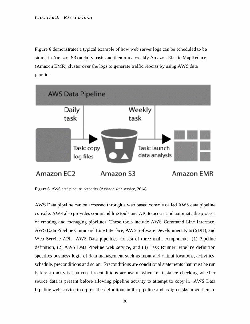
Figure 6 demonstrates a typical example of how web server logs can be scheduled to be

stored in Amazon S3 on daily basis and then run a weekly Amazon Elastic MapReduce

(Amazon EMR) cluster over the logs to generate traffic reports by using AWS data

pipeline.

Figure 6. AWS data pipeline activities (Amazon web service, 2014)

AWS Data pipeline can be accessed through a web based console called AWS data pipeline

console. AWS also provides command line tools and API to access and automate the process

of creating and managing pipelines. These tools include AWS Command Line Interface,

AWS Data Pipeline Command Line Interface, AWS Software Development Kits (SDK), and

Web Service API. AWS Data pipelines consist of three main components: (1) Pipeline

definition, (2) AWS Data Pipeline web service, and (3) Task Runner. Pipeline definition

specifies business logic of data management such as input and output locations, activities,

schedule, preconditions and so on. Preconditions are conditional statements that must be run

before an activity can run. Preconditions are useful when for instance checking whether

source data is present before allowing pipeline activity to attempt to copy it. AWS Data

Pipeline web service interprets the definitions in the pipeline and assign tasks to workers to


27

move and transform data. The Task Runner polls the AWS Data Pipeline web service for

tasks and then performs those tasks. As shown in Figure 6, Task Runner copies log files to

Amazon S3 and then launches Amazon EMR clusters.

As Azure data factory supports data transformation through Hive, Pig, and custom C#

processing in Hadoop, it allows the MapReduce pattern to parallelize data transformation

which can automatically scale when data grow. Hive and Pig generate MapReduce functions

and run them behind the scenes to carry out the requested query. Table 1 presents features

comparison between the AWS and Azure data pipelines. The pricing associated with ADF

based ETL is discussed in Section 5.5.

Table 1: Basic features comparisons between AWS and Azure Data pipelines

Features Azure AWS Alternative

Dependent chain of data source ✓ ✓

scheduling pipeline activities ✓ ✓

running and monitoring activities ✓ ✓

Built-in activities common action such as

copying data from storage system of own

platform

✓ ✓

Creating pipelines from portal ✕ ✓ Azure PowerShell

CHAPTER 3. IMPLEMENTED DATA FACTORY FOR DATA QUALITY MANAGEMENT

28

Chapter 3

Implemented Data Factory for data quality management

In this Chapter, the architecture implemented for data quality management is described. This

Chapter explains how Azure Data Factory (ADF) can be used to build a robust, automated,

and scalable ETL system leveraging parallel processing and machine learning. The proposed

ADF for data quality management system works in the following set up. Raw data is stored

in Azure Blob store, Hadoop clusters provided by HDInsight and Hive scripts are used for

data processing, Azure ML studio is used for applying statistical function by running custom

R scripts. Finally, the cleaned data is stored in MS SQL database. A brief description of how

an ADF project for data quality management was built and deployed is presented. This

includes the description of the processes of integrating storage and compute service with

ADF, setting data cleaning rules, and scheduling the data pipeline to perform data cleaning

and data movement tasks. Some code snippets are shown to describe technical aspects of the

implementation.

The implemented architecture supports performing a number of tasks such as picking raw

data from Azure Blob Store, processing the raw data using Hadoop clusters and hive scripts,

processing data via a web service provided by Azure Machine Leaning Studio (ML Studio),

and moving data from Azure Blob store into Azure MS SQL. In short, the key components

of the proposed architecture are ADF, Azure storage, HDInsight, ML Studio, and MS SQL.

Section 3.1 through 3.3 describe these components in detail and explains how these

components fit in the proposed architecture for data quality management. Section 3.2

presents the diagram views of the proposed architecture and give a brief description of some

of the code snippets taken from the deployed data quality management systems built around

the proposed architecture. Detailed descriptions of how sample data was processed using this

architecture are presented in Chapter 4. The major components of the ETL are discussed

individually before presenting the complete architecture. The proposed architecture is

discussed in Section 3.2.


29

3.1 Creating ADF

As discussed in Section 2.2.2 ADF plays a central role in creating ETL system on Azure

platform. ADF helps connect required components of ETL such as Azure blob for storing

raw telemetry data, HDInsight for parallel data processing (cleaning), and ML Studio for

applying machine learning models against the raw data, and SQL database for storing the

cleaned data. This is why, creating the ADF pipeline is the very first step towards building

the complete architecture of the ETL.

Creating and deploying ADF requires an Azure account. There are several purchase options

available to get one (Purchase options for Azure Account 2014). During this thesis work,

MSDN subscription was used. ADF can be created either from Azure preview portal or by

using Microsoft Azure PowerShell. Creating ADF also requires defining a ResourceGroup

for the ADF. Azure PowerShell has a command line interface that supports commands related

to ADF. Some of the actions such as creating and scheduling pipelines cannot be performed

through Azure preview portal. For such actions, Azure PowerShell can be used. However,

making Azure preview portal independent so that all the actions can be performed through

azure preview portal itself would be a big advantage.

ADF consists of two key components: linked services and pipelines. These components

enable ADF to connect with other services and run scheduled jobs. Linked services help to

connect other services available on Azure platform with ADF. Once these services are

connected to ADF via linked services, pipelines can be scheduled to perform certain tasks

including processing data or moving data from one source to another. The first step however

is to create ADF. Next, creating linked service, pipelines, and scheduling pipelines follow

respectively. For example, once ADF is created, it can be linked with Azure Blob Store and

MS SQL and then a pipeline can be created to copy data from Azure Blob to MS SQL.


30

Further, to automate this data movement, the pipeline can be scheduled to perform this task

of copying data from Azure Blob to MS SQL daily at a given time.

The linked service can be created either from graphical interface (Azure preview portal) or

Azure PowerShell which is a command line interface. However, Azure preview portal only

supports creation of linked services for Azure Storage account, Azure SQL, and SQL Server.

Scripts should be written in JSON and should be uploaded to ADF using Azure PowerShell

to create linked services for HDInsight or Azure ML Studio. HDInsight and ML Studio are

covered in Section 3.1.2 and 3.1.3 respectively. As this thesis work aimed to propose an

architecture for data quality management system built around ADF and other services

available on Azure platform. The key services that were found to be promising and were used

to construct the architecture for data quality management system are discussed in Section

3.1.1 through Section 3.1.4.

3.1.1 Windows Azure Storage

Windows Azure Storage (WAS) is a scalable cloud storage (Calder et.al 2011) that provides

cloud storage. Data can be stored in the form of containers (blobs), tables (entities), queues

(messages), and shares (directories/files) in WAS (Azure Storage 2015). WAS is massively

scalable, durable, and highly available in nature. For this reason, WAS fits well to Big Data

scenarios and hence it fits for the architecture this thesis work aims to propose. A standard

storage account provides unique namespace for storage resources including Blob, Table,

Queue, and File storage. The sample telemetry data used in this thesis work was in the form

of text file which was suitable for storing in Azure Blob. Using the storage account, a Blob

container was created and sample data was uploaded there. ADF also allows to keep the hive

script in Azure Blob. The Hive scripts for processing the raw data (sample telemetry data)

was also stored in Blob.


31

3.1.2 Azure HDInsight

Azure HDInsight is a framework for Microsoft Azure cloud implementation of Hadoop

(Sarkar 2014). HDInsight includes several Hadoop technologies. To name a few, HDInsight

includes Ambari for cluster provisioning, management, and monitoring; Avro for data

serialization for Microsoft .NET environment; HBase which is a non –relational database

for very large tables, HDFS, Hive for SQL-like query; Mahout for supporting machine

learning; MapReduce and YARN for distributed processing and resource management; Oozie

for workflow management; Pig for simpler scripting for MapReduce transformations; Scoop

for data import and export; Strom for real-time processing of fast, large data streams; and

Zookeeper for coordinated processes in distributed systems (Microsoft Azure, 2015)

Accessing a cluster usually means accessing a Head Node or a Gateway which is a setup to

be the launching point for the jobs running on the cluster (zhanglab 2015). Clusters on

HDInsight can also be accessed in similar fashion. HDInsight can be considered as fully

compatible distribution kit of Apache Hadoop which is accessible as platform as service on

Azure. As highlighted by the Sysmagazine (2015), one of the most noticeable contributions

to apache Hadoop ecosystem are the development of Windows Azure Storage Blob (WASB).

The WASB provided a thin interlayer to represent units of blob storage of Windows Azure

in the form of HDFS cluster of HDInsight (Sysmagazine 2015.) Figure 7 illustrates the

internal architecture of HDInsight cluster.


32

Figure 7: Internal Architecture of HDInsight cluster (Sysmagazine 2015)

As illustrated by Figure 7, a job has to pass through Secure Role first. Secure Role are

responsible for three main tasks: 1) authentication, 2) authorization, and 3) giving finishing

points for WebHcat, Ambari, HiveServer, HiveServer2 and Oozie on port 433. Head Node

works as a site presented by virtual machines of level of Extra Large (8 kernels, 14 GB RAM)

and fulfils the key function of Name Node, Secondary NameNode, and JobTracker of

Hadoop cluster. Worker Nodes work as sites presented by virtual machines of level of Large

(4 kernels, 7 GB RAM). Worker Nodes start tasks that support scheduling, execution of tasks

and data access. WASB is in the form of HDFS. It is the default file system for HDInsight

(Sysmagazine 2015.) As a result, HDInsight can access the data stored in Azure storage.

ADF can be linked to HDInsight in order to process data by running Hive/Pig scripts or

MapReduce programs. For the ETL process, this enables programmers to schedule data

cleaning jobs through ADF’s pipelines that can process data by running Hive/Pig scripts or

MapReduce program in HDInsight clusters. During this thesis work, Hive scripts were used

to perform data cleaning in the HDInsight clusters. Hive facilitates querying and managing

large datasets residing in distributed storage (Apache Hive 2015). Since Hive runs on top of

MapReduce and has syntax very much like SQL, it eases programmers’ life who prefer SQL

like query language over MapReduce. For this reason, Hive was chosen for this thesis work.


33

However, the implemented ADF is not limited to Hive. During the data cleaning process, the

cleaned datasets were stored back in the Azure Blob store so that other data cleaning rules

can be applied if need.

3.1.3 Azure ML Studio

A number of publications in the area of Big Data analysis highlight the applicability of

machine learning: “Developing and testing machine learning architecture to provide real-

time predictions or analytics for Big Data” (Baldominos & Albacete & Saez & Isasi 2014),

“A survey on Data Mining approaches for Healthcare” (Tomar & Agarwal 2013), “Big Data

machine learning and graph analytics” (Huang & Liu 2014) and many more. Mining Big

Data usually requires various technical approaches that include database system, statistic,

and machine learning. Therefore, the ETL system designed to work in the Big Data scenarios

should support these technical approaches. Machine learning is one of the most important

applications of Big Data.

To support machine learning in the ETL process, the implemented data factory for data

quality management proposed in this thesis work, integrates Azure ML Studio. Azure ML

Studio is a recently announced (July, 2014) Machine Learning service of Microsoft Azure.

ML Studio is a collaborative visual development environment that allows building, testing

and deploying predictive analytics solutions as web service. ML Studio as shown in Figure

8 below can read data from various sources and formats.


34

Figure 8: Overview of Azure ML Studio (Microsoft Azure 2015)

Azure ML Studio allows to extract data from various sources and transform and analyze that

data through a number of manipulation and statistical functions in order to generate results.

Azure ML Studio provides interactive canvas where datasets and analysis modules can be

dragged- and dropped. There are several data transformation functions, statistical functions

and machine learning algorithms available in ML Studio. These include Classification,

Clustering, and Regression, Cross Validate Model, Evaluate Model, Evaluate Recommender

Model, Assign to Cluster, Score Model, Train Model, Sweep Parameters and many more. In

addition, custom R scripts can be run against datasets. A custom R script was used to calculate

confidence interval during this thesis work. The R script is presented in Section 3.1.4. Figure

9 shows the experiment created for calculating confidence interval from a sample data stored

at Azure Blob store. The experiment was then published as web service and tested.


35

Figure 9: Experiment created and published as web service for calculating confidence interval

Figure 9 can be read in four main steps. Each step is represented by a component of ML

Studio which was dragged from the tool-bar into the workspace and configured. Each

component has input and output port for accepting data and outputting data. The arrows in

the Figure shows where the input data for a component comes from and where the output

goes. In the first step, the source data is read from Azure Blob store. Reading data from

Azure blob can be done by dragging the Reader component from the tool bar to work space

in ML studio and configuring the reader component for accessing the Azure blob store and

files stored in there. Configuration requires Azure Blob store account credentials and path of

the input file inside the Azure Blob container. In the second step the data type of a column

containing missing value, is converted into double. This is required because ML Studio


36

requires the column type to be double before the missing values in it can be replaced with

‘NaN’. ML Studio has a dedicated component for doing this task. In the third step, the

missing values are replaced with ‘NaN’ by using available component. In the fourth step, 95

percent confidence intervals are calculated against the input data. For running R script against

input data, ML Studio has a dedicated component which can be dragged into the work space

which then gives input area for writing custom R script. Below is the R script that was used

to calculate 95 percent confidence intervals.

# Map 1-based optional input ports to variables

1 data.1 <- maml.mapInputPort(1) # class: data.frame

#Create the matrix for output (as many rows as in the input file)

2 output.1 <- matrix(NaN, ncol=3, nrow=nrow(data.1))

3 output.1<-data.frame(output.1)

#Check which rows involve missing OK.count or missing Reset.count –returns either true or false

(boolean)

4 na.rows <- which (is.na(data.1$OK.count) | is.na(data.1$Reset.count))

#Assign the row count to parameter n.rows --

5 n.rows <- nrow(data.1)

#Create the set of rows to be scanned by binom.test function

6 scan.rows <- setdiff(c(1:n.rows), na.rows)

#Create a loop that performs the test

7 for(i in scan.rows) {

8 bin.test <- binom.test(x=c(data.1$OK.count[i], data.1$Reset.count[i]),n=1, conf.level=0.95)

9 conf.int.i.estimate <- bin.test$estimate

10 conf.int.i.lower <- bin.test$conf.int[1]

11 conf.int.i.upper <- bin.test$conf.int[2]

12 output.1[i,] <- cbind(conf.int.i.estimate, conf.int.i.lower, conf.int.i.upper)

13 }

#Add descriptive column and row names to the output matrix

14 colnames(output.1) <- c("Actual", "CI.lower", "CI.upper")

15 rownames(output.1) <- data.1$Trial.id

16 maml.mapOutputPort("output.1");


37

3.1.4 Azure SQL Database

Azure SQL database version V12 provides complete compatibility with Microsoft SQL

Server engine as claimed by Azure. This version of Azure SQL allows users to create

databases from Azure preview portal (MightyPen 2015.) ADF provides linked service and

pipeline supports to connect with Azure SQL and run pipelines. During this thesis work,

Azure SQL was used to store the cleaned data. Azure SQL database was linked with ADF

using linked service. Tables were created in Azure SQL database for each of the cleaned

datasets. ADF’s copyActivity was used to copy the cleaned data from Azure Blob store to

Azure MS SQL database.

3.2 Proposed Architecture

Several steps were taken to ensure the reliability and validity of the architecture before

making the proposition. The first step was to study, explore, and test the potential components

independently. In the second step, all those components were connected to ADF one by one

and tested. For example, firstly, sample data was placed in Azure Blob and a table was created

in Azure SQL database and then both Azure Blob storage and Azure SQL were connected to

ADF via linked service and a pipeline was run to copy the data residing in Azure Blob to

Azure SQL database table. After this experiment was successful, tables and pipelines scripts

were updated to address more requirements.

Then next step was to integrate HDInsight with ADF. This was essential for processing data

using Hadoop cluster provided by HDInsight. HDInsight was connected to ADF in similar

fashion as Azure Bob and Azure SQL database were connected. The Hive script required to

run against the sample data to get desired output was stored in Azure Blob. When creating

linked service for HDInsight, cluster size, the path for accessing the Hive script residing in

Azure Blob were defined. Also, clusters were configured to be of type On-demand cluster to

avoid unnecessary costs. ADF allows users to configure HDInsight via linked service in such

a way that depending on the schedule of the pipeline, Hadoop cluster can be set up

automatically. Further, when pipelines finish running, the cluster can be shut down


38

automatically. This can save a lot of cost especially when the pipelines are running once a

day because often all the jobs can be finished within a couple of hours. The Hive scripts

contained only a few data cleaning rules in the beginning. After this experiment was

successful, the Hive scripts were refined and remaining data cleaning rules were added in

sequential order. At this point, a highly robust, scalable, and reliable data quality

management system had been built which could be used to clean massive amount of data.

Since the data cleaning rules were applied in sequential order, it became quite modular and

it was easy to add a new rule or drop existing ones without affecting the whole architecture.

The final step was to add machine learning capabilities to this ADF.

During this thesis work, there was a recent update done in ADF by Azure which allowed to

connect Azure ML Studio to ADF via linked service and also pipeline support was added.

This was a great opportunity to add machine learning capabilities to the data quality

management system being developed. The experiment discussed in section 3.1.3 and shown

in Figure 9 was created and R script was run against sample data stored in Azure Blob to

calculate CI. Further, the experiment was published as web service. Finally ADF was then

connected to this web service utilizing the recent update made by Azure. Figure 10 shows

the complete architecture of the proposed data quality management system.

Figure 10: An architecture of implemented data factory for data quality management


39

As can be seen from Figure 10, first, pipeline picks raw data from Azure blob and processes

the data in HDInsight clusters by running hive scripts. The results are stored in Azure Blob.

Results are furthers transformed by using Azure ML Studio. The results are stored back in

Azure blob in separate directory. Finally, the cleaned data is copied to Azure SQL database.

The Telemetry UI reads data from Azure SQL database and presents them in various visual

charts and tables.

In some cases, more than one service was found on Azure platform which could serve the

same purpose. In such cases, the services which looked more current, scalable, and well-

suited for ADF and business case of the client company, were chosen. For example, there

was possibility to use Mahout for machine learning. However, the Azure ML Studio turned

out to be easy to implement yet very powerful. For this, reason ML Studio was chosen over

Mahout. Similarly Hive was chosen over Pig as the current database of the client company is

MS SQL and developer of the case company showed more interest towards Hive than Pig. The

reason was that Hive’s syntax is identical to SQL.

3.3 Deployment of the data quality management system

MSDN account can be used to get access to Azure preview portal which allows to create

ADF and integrate other services such as HDInsight, Azure SQL database, Azure Blob store,

and Azure ML Studio. However, only limited work such as creating ADF and linked services

for MS SQL and Azure Storage can be done from the ADF preview portal. For the rest of the

work including creating linked services for HDInsight, Azure ML Studio, creating pipelines,

uploading input and output table schemas, scheduling pipelines are done by using Azure

PowerShell. To upload raw data and Hive scripts in Azure Blob store, CloudBerry Explorer for Azure

Blob Storage can be used.

Despite the fact that it is possible to create ADF and certain linked services from ADF

preview portal, it is recommended to use an Integrated Development Environment (IDE). It

is also more convenient to create a project and code all the components inside a single project


40

on the local machine than doing everything from the preview portal. This allows

collaborating with other developers via version control. In addition, it makes it easier to

maintain and update the ADF. During this thesis work, Sublime Text 2 was used as IDE and Git

was used as version control. Azure PowerShell can be used to deploy the tables, pipelines,

linked services of ADF from local machine to ADF in the cloud. During this thesis work,

ADF and linked services for Azure SQL, and Azure Storage were created from ADF preview

portal and the rest were coded locally and deployed using Azure PowerShell. As an example,

let us imagine we want to deploy a new pipeline named “batChargeTimeRule” which resides in

a file called “batChargeTimeRule.json” on the local machine. Assuming the file is in current

directory, the following command can be used to deploy the pipeline from local machine to

ADF named “TestDataFactory” with ResourceGroupName “TestResourceGroup”.

1 New-AzureDataFactoryPipeline –ResourceGroupName TestResourceGroup -DataFactoryName

TestDataFactory -File batChargeTimeRule.json

Figure 11 shows the diagram view of the final deployment of the implemented ADF that

serves as the data quality management system. As a result of this deployment, we would

now have a rule in place to remove battery charge data where the time taken to charge the

device was much lower than would be physically possible.


41

Figure 11: Diagram View of Implemented data factory for data quality management


42

ADF preview portal allows to visually see input/output tables and pipelines and visualize

how data passes through different data cleaning rules and finally gets stored in SQL table. It

is possible to see the table schemas and pipeline definitions by double clicking the table or

pipelines. E.g., in Figure 11, HiveInputBlobTable is an on read table schema for sample data. A

batDischarge pipeline takes that table as an input. The batCharge pipeline contains an activity

which runs Hive scripts against the sample data inside HDInsight and creates batDischarge table.

At this point only discharging events have been separated from the sample data and placed

in batDischarge table. No data cleaning rule has been applied yet. Further, the next pipeline

batDischargeTimeRule takes batDischarge table as input and its activity runs Hive script containing

data cleaning rule that filters all the discharge time events where discharge time is 0 or

negative and places the cleaned data in a table batDischargeTimeRule. Then, a pipeline

batDischargePercentLossRule takes batDischargeTimeRule as input and applies data cleaning rule

which filters out all the cases where percent loss contains negative value and places the

cleaned data in batDischargePercentLossRule table. Later, another pipeline

batDischargeCapLossRule takes batDischargepercentLossRule table as input and applies a data

cleaning rule that filters out all the cases where battery capacity loss contains negative values

and places the cleaned data in batDischargeCapLossRule table. Finally, as there is no other rule

to apply, batDischargeCapLossRule table contains the final cleaned data and hence this table is

copied to the Azure SQL table batDischargeSQL via another pipeline batDischargeSQL.

Below are sample code snippets that were used to connect with HDInsight and set up On-

demand clusters. Sensitive information such as username, password etc. have been replaced

by a placeholder and presented within angle brackets.

1 {

2 "Name": "MyHDInsightCluster",

3 "Properties":

4 {

5 "Type": "HDInsightBYOCLinkedService",

6 "ClusterUri": "https://<clustername>.azurehdinsight.net/",

7 "UserName": "<Username>",

8 "Password": "<Password>",

9 "LinkedServiceName": "<Name of Linked Service>"

10 }

11 }

Code snippet of linked service for connecting ADF to HDInsight


43

The code snippet shown above was used to connect to HDInsight and create a Hadoop cluster.

The developer can choose username and password at this point when provisioning the cluster.

It is advisable to give a meaningful cluster name and linkedServiceName. The next step is to

configure clusters.

1 {

2 "name": "HDInsightOnDemandCluster",

3 "properties":

4 {

5 "type": "HDInsightOnDemandLinkedService",

6 "clusterSize": "4",

7 "jobsContainer": "adfjobs",

8 "timeToLive": "02:00:00",

9 "linkedServiceName": "<Name of Linked Service>"

10 }

11 }

Code snippet of linked service for setting up On-demand clusters

In the above shown code snippet, the cluster is configured to be an On-demand cluster. On-

demand cluster means, HDInsight will set up the cluster when the pipeline requires to run jobs.

Once the jobs are finished, the cluster is shut down to cut the unnecessary costs. As can be

seen, the cluster size was defined to be 4. This can be configured depending on the volume

of the data which needs to be processed or can be left blank in which case HDInsight will

decide the cluster size depending on the volume of the data given. JobsContainer is a container

for example in Azure blob to accommodate all the MapReduce jobs and outputs. When using

On-demand clusters, one might not want to shut down the cluster as soon as the job is finished

so as to get some time to analyze the results and if needed tweak the Hive script and re-run

the jobs (by running pipeline). This is important because HDInsight roughly takes about 20

minutes to set up the cluster and allocate the needed resources before it can run any data

processing job. Once the cluster is set up and resource is allocated, running jobs only takes

about a minute or two depending on the complexity of query and volume of data, and cluster

size. Developer can set timeToLive so that when the job is finished, output can be analyzed and

if needed Hive script can be tweaked and re-run the job without having to wait for another

20 minutes for HDInsight to setup cluster all over again. For this reason, timeToLive was set to

be 2 hours as shown in the code snippet above. In the similar fashion, ADF can be linked

with Azure SQL Database, Azure ML Studio.


44

As described in section 2.6.1 data pipelines are groups of data movement and processing

activities that can accept one or more input datasets and produce one or more output datasets.

Data pipelines can be executed once or can be scheduled to be executed hourly, daily, weekly

and so on. Like linked services, pipeline definitions are defined in the JSON and uploaded to

ADF via Azure PowerShell. Below is an example code snippet of a pipeline that takes

batCharge as input and produces batChargeTimeRule as output by running Hive script against the

input data.

1 {

2 "name": "batChargeTimeRule",

3 "properties":

4 {

5 "description" : "It runs a Hive query and stores the result set in a blob",

6 "activities":

7 [

8 {

9 "name": "RunHiveQuery",

10 "description": "Applies data cleaning rule that filters out chargtime < 1",

11 "type": "HDInsightActivity",

12 "inputs": [{"name": "batCharge"}],

13 "outputs": [ {"name": "batChargeTimeRule"} ],

14 "linkedServiceName": "HDInsightOnDemandCluster",

15 "transformation":

16 {

17 "type": "Hive",

18 "extendedProperties":

19 {

"RESULTOUTPUT":"wasb://<ContainerName>@<Storagename>.blob.core.windows.net/table

s/battery/hiveoutput/chargingtable/batChargeTimeRule.txt",

21 "Year":"$$Text.Format('{0:yyyy}',SliceStart)",

22 "Month":"$$Text.Format('{0:%M}',SliceStart)",

23 "Day":"$$Text.Format('{0:%d}',SliceStart)"

24 },

25 "scriptpath": "<ContainerName>\\scripts\\battery\\charging\\batChargeTimeRule.hql",

26 "scriptLinkedService": "Name of the Linked Service"

28 },

29 "policy":

30 {

31 "concurrency": 1,

32 "executionPriorityOrder": "NewestFirst",

33 "retry": 1,

34 "timeout": "00:30:00"

35 }

36 }

37 ]

38 }

39 }

Code snippet of pipeline that runs hive scripts in HDInsight

20

0


45

In the given above code snippet, the type of the activity for this pipeline has been defined to

be HDInsightActivity. The HDInsightActivity allows for the running of Hive scripts. The hive

scripts can be stored in Azure Blob Store. The location of the hive script can be defined in

the pipeline as scriptpath as shown in the code snippet above. The directory where the output

is stored can be defined under RESULTOUTPUT. The wasb syntax is used to access Windows

Azure Storage Blob which is followed by

[email protected]/NameOfDirectory. When this

pipeline runs, it takes batCharge as its input table, sets up the OnDemand Cluster as defined

under linkedServiceName, and runs the hive script picking it from location specified under

scriptpath. The script performs data cleaning based on the rule defined in it and stores the

output in batChargeTimeRule table and finally uploads the output table to the location

specified under RESULTOUTPUT.

CHAPTER 4. TESTED SAMPLE DATA

46

Chapter 4

Tested sample data

In this Chapter a brief description of the sample data used in this thesis work is given. Further,

this Chapter introduces the identified data quality problems of the sample data of the client

company and discusses how data cleaning rules were selected, applied, and assessed.

4.1 Sample data source

The sample data used in this thesis work is telemetry data of mobile devices particularly

about battery. This data was made available by the client company. The data is captured as

charging and discharging sessions through a feedback application installed on users’ mobile

devices. Whenever a user plugs in a phone for charging or disconnects a phone from

charging, an event is generated. Charging and discharging events are identified by the value

recorded under CycleType data field. For example, value 1 is recorded for charging events

and value 2 is recorded for discharging events. Charging/discharging events not only record

the current percentage of battery but also many other pieces of information about the device.

E.g., charging events includes data including device id, charge time, charger type, percentage

of battery that increased during the charging session, capacity of the battery, percentage of

battery capacity that increased during the charging session, and battery temperature recorded

at the end of the charging session. This is very valuable data for a company producing and

selling mobile devices. This data can be used to measure the performance of the battery and

enhance the user experiences by identifying the problem area and improving them.

To examine how false positives in automatic data cleaning can be minimized, this sample

telemetry data was cleaned utilizing the data quality management system built based on

architecture proposed in Section 3.2. Automation of data cleaning was achieved by

implementing data pipelines provided by Azure Data Factory. For the purpose of validating

the architecture, some of the known issues in the sample telemetry data were addressed in


47

data cleaning process. There were altogether 34 fields in the given sample. The relevant fields

in the raw data which were used in the data cleaning process are shown in table 2.

Table 2: Relevant fields of the sample data used in analysis

Fields Value Explanations

cycleType 1 or 2 1 represents charging events and 2

represents discharging events

CycleResultCode 1 or 2 1 represents charging events and 2

represents discharging events

CycleTimeSeconds Integer If CycleType is equal to 1, then

CycleTimeSeconds represents

charging time else if CycleType is

equal to 2 it represents

discharging time

CycleBatteryStart_Pct Integer Represents battery % when

charging started

CycleBatteryEnd_Pct Integer Represents battery % when

charging stopped

CycleCapacityStart_mWh Integer Represents available battery

capacity when charging started

CycleCapacityEnd_mWh Integer Represents battery capacity when

charging ended

ClientSessionStartDateTime

DateTime When charging/discharging

started

ClientSessionEndDateTime DateTime When charging/discharging ended


48

4.2 Known issues in sample data

The sample data contained dirty data. This can partly be expected as batteries are physical

objects which degrade in performance over time. There are also physical interfaces in the

devices which may not work as well with some 3rd party provided batteries and lead to poor

measurements. The client company gets this data on a daily basis and uses it for

understanding a number of different aspects related to power consumption. For instance, the

date helps understand battery performance against different firmware versions, charging

behavior of users for example when people charge their phone more often, types of charger

people mostly use and so on. The client company stores this data in a MS SQL database. The

client company has a web portal that reads data from database and presents data in visual

form such as graphs and tables. The client company is aware that only good quality data can

lead to good decisions. Consequently, the client company performs data cleaning on daily

basis to maintain the quality of data. However, this is a lengthy task as the volume of the data

the case company gets is expected to grow massively in near future. This explains the need

for automated data cleaning. The architecture proposed in this thesis work supports

automated data cleaning and therefore can tackle this issue. The known issues in the sample

telemetry data which were addressed during data cleaning are as follows:

Charge time contains cases with negative value

Discharge contains cases with negative value

Referring to the above table 2, battery % gain for charge time is calculated by

subtracting CycleBatteryEnd_Pct from CycleBatteryStart_Pct. For the scenario

where a device consumes more battery than it gains from charging (E.g., when user

is playing video game and Wi-Fi is turned), battery % gain is captured as negative

value. So there are certain extreme scenarios where devices can be charging but are

consuming power faster than they gain power via re-charging. However, it was

captured during data cleaning process to observe how frequent such cases are.


49

In some cases battery % increases with positive charge time but battery capacity does

not increase. Capacity gain is calculated in similar fashion as battery % gain by

subtracting CycleCapacityStart_mWh from CycleCapacityEnd.

In some cases with positive charge time battery capacity increases but battery %

gain does not increase

Charge loss is negative. Charge loss is calculated subtracting CycleBattryEnd_Pct

from CycleBatteryStart_Pct.

With the existing errors in the sample data listed above, it would be quite risky to make

product related decisions as there is high risk of ending up making wrong decisions. For

example, predicting the average battery life of a phone from datasets which contain such

garbage data can result into a false positive. In their description of the problems that dirty

data can cause when making decisions (Chiang & Miller 2008) warns that dirty data is a

serious problem for business leading to incorrect decision making, inefficient daily

operations, and ultimately wasting both time and money. Application of data quality rules

(Chiang et. al 2008) is the common rule of thumb for identifying and cleaning dirty data from

datasets.

For the selection of data cleaning rules, this thesis work adapted with the approach proposed

by (Hoa & Chun 2008). This approach consists of five parts which are: (1) rules definition,

(2) data quality problem definition, (3) cleaning results assessment, (4) rules performance

storage, and (5) rules scheduling. Hoa (2008) advocates for speed when measuring rules

performance. However, this thesis work also aims to measure the false positive rate of data

cleaning rules when measuring the rules performance. This can help minimize the false

positive rate of the data cleaning rules through multiple iteration. Figure 12 illustrates the

adapted optimal cleaning rule selection model.


50

Figure 12: Optimal cleaning rules selection model (adapted from Hoa & Chun 2008)

To get an idea of how much data can be filtered out when data cleaning rules are applied for

the known issues in sample data, two different tables 'batChargeViolation' and

‘batDischargeViolation’ were created in MS SQL database to hold % percent of data that each

rule related to charging and discharging can filter. Then using the proposed architecture a

pipeline was run which picked the sample data from Azure blob, ran the Hive script against

it in HDInsight, and finally copied the results to 'batChargeViolation' and ‘batDischargeViolation’

tables of MS SQL. This was done for seven different sample datasets to observe how results

changed over time. This gave a benchmark for evaluating potential data cleaning rules to

address the known issues in the sample data. Table 3 shows the evaluated potential data

cleaning rules, their description and the portion of hive script needed.


51

Table 3: Potential data cleaning rules for battery related telemetry data

Potential Data cleaning

rules

Description Hive script

Charge time rule Calculates the total % of

cases where charge time <

1 second

ROUND(SUM(CASE WHEN CycleTimeSeconds < 1

and CycleType=1 and CycleResultCode=1 THEN 1

ELSE 0 END)*100/SUM(CASE WHEN CycleType=1

and CycleResultCode=1 THEN 1 ELSE 0 END),2) AS

ChargeTimeRule

Discharge time rule Calculates the total % of

cases where discharge time

< 1 second

ROUND(SUM(CASE WHEN CycleTimeSeconds < 1

and CycleType=2 and CycleResultCode=2 THEN 1

ELSE 0 END)*100/SUM(CASE WHEN CycleType=2

and CycleResultCode=2 THEN 1 ELSE 0 END),2) AS

DischargeTimeRule

Charge % gain rule Calculates the total % of

cases where charge % gain

< 1

ROUND(SUM(CASE WHEN CycleType=1 and

CycleResultCode=1 and (CycleBatteryEnd_Pct-

CycleBatteryStart_Pct) < 1 THEN 1 ELSE 0

END)*100/SUM(CASE WHEN CycleType=1 and

CycleResultCode=1 THEN 1 ELSE 0 END),2) AS

ChargeGainRule

Charge % loss rule Calculates the total % of

cases where charge % loss

< 1


CycleResultCode=2 and (CycleBatteryStart_Pct-

CycleBatteryEnd_Pct) < 1 THEN 1 ELSE 0

END)*100/SUM(CASE WHEN CycleType=2 and

CycleResultCode=2 THEN 1 ELSE 0 END),2) AS

ChargeLossRule

Charge % gain error rule Calculates the total % of

cases where charge time >

0 and there has been

capacity gain but not

percent gain


CycleResultCode=1 and CycleTimeSeconds > 0 and

(CycleCapacityEnd_mWh-CycleCapacityStart_mWh) >

0 and (CycleBatteryEnd_Pct-CycleBatteryStart_Pct) < 1

THEN 1 ELSE 0 END)*100/SUM(CASE WHEN

CycleType=1 and CycleResultCode=1 THEN 1 ELSE 0

END),2) AS ChargePercentGainErrorRule

Capacity gain error rule Calculates the total % of

cases where charge time >

0 and there has been

percent gain but not

capacity gain


CycleResultCode=1 and CycleTimeSeconds > 0 and

(CycleBatteryEnd_Pct-CycleBatteryStart_Pct) > 0 and

(CycleCapacityEnd_mWh-CycleCapacityStart_mWh) <

1 THEN 1 ELSE 0 END)*100/SUM(CASE WHEN

CycleType=1 and CycleResultCode=1 THEN 1 ELSE 0

END),2) AS CapacityGainErrorRule


52

Seven days results from both the tables are presented in Chapter 5. Figure 13 shows the

results obtained from charge time and percent gain rules. Figure 14 shows the results

obtained from discharge time and percent loss rules, and Figure 15 shows the results of

percent gain error and capacity gain error rules.

Figure 13: Seven days results of Potential charge time and Percent gain rules

As can be seen from the Figure 13, during the seven days period, total % of cases where

charge time < 1 second is between 0.25% to 0.5 %. During the same period of time, the cases

where charge percent gain < 0 is between 0.75% to 1.25%.


53

Figure 14: Seven days results of Potential discharge time and Percent loss rules

Figure 14 shows that cases discharge time rule has caught is below 2.5 %. Percent loss rule

seems to be quite problematic. Applying percent loss rule in data cleaning can filter out about

12 % of total discharging data. Therefore, it would be wise to consider further evaluation of

percent loss before deciding to apply it in data cleaning. For example, this could be happening

due to some hardware problems or temperature of the phone.

Figure 15: Seven days results of Potential percent gain error and capacity gain error rules


54

As shown in Figure 15, percent gain error is significantly nominal in comparison with

capacity gain error. This figure points out a serious issue with capacity gain error. Referring

to the description of capacity gain error presented in Table 3, capacity gain error rule

calculates the total % of cases where charge time > 0 and there has been percent gain but not

capacity gain. This issue with capacity gain error can cause false positives for example if

included in calculating the total charge time required for a phone's battery to be fully charged.

This figure also points out that using percent gain instead of capacity gain when predicting

total time required for a phone's battery to fully charge is less risky.

4.3 Data quality problems and data cleaning rule definitions

Quality problems in the sample data were already known. Evaluating potential data cleaning

rules against 7 days of datasets helped better understand the possible impact these rules can

have. Observing the capacity gain error, it was clear that percent gain and capacity gain are

out of sync. Applying a data cleaning rule to filter negative capacity gain can filter a

significant amount of data. This was already an indication that percent gain should be

preferably used over capacity gain when drawing any conclusion from the data. Data cleaning

rules for charging and discharging events were defined based on the listed known issues of

the sample data and the evaluation of the potential data cleaning rules. Further, these data

cleaning rules were assigned a priority order for their sequential application. Priority order

was assigned based on the amount of data a rule could potentially filter out. The rule that

would filter the least amount of data got first position in sequential order of the rule. Using

priorities for the cleaning rules helped to minimize the amount of data being lost when

applying filters and this was important as more data gave better and reliable results. Table 4

shows the defined data cleaning rules and their priority order.


55

Table 4: Defined data cleaning rules and their priority orders

Data cleaning rules for charging events

Data cleaning rules Description Priority order

ChargeTimeRule Filters out charge events having charge time <=0 1

PercentGainRule Filters out charge events having percent gain <0 2

CapacityGainRule Filters out charge events having capacity gain <=0 3

Data cleaning rules for discharging events

Data cleaning rules Description Priority order

DischargeTimeRule Filters out discharge events having discharge time <=0 1

PercentLossRule Filters out discharge events having percent loss <0 2

CapacityLossRule Filters out discharge events having capacity loss <=0 3

4.4 Assessment of data cleaning rules

Assessment of the data cleaning rules was done against the performance of the rules. To

assess the performance of the data cleaning rules, false positive rate was calculated for each

of the applied rules. As suggested by Hoa (2008), the false positive rate can be calculated by

counting the number of wrongly identified rows over total identified rows multiplied by 100.

The same approach suggested by Hoa (2008) was used in this thesis. Further, the 95 percent

confidence interval (CI) was calculated for each of the data cleaning rules to observe the

possible variation in false positive rate when applying the rules to different sizes of datasets.

Chapter 5 presents the process of defining the criteria for false positive and the process of

calculating 95 percent CI.

CHAPTER 5. RESULTS AND EVALUATIONS

56

Chapter 5

Results and Evaluations

In this Chapter, the results of running tests on the sample data are discussed. The sample data

was tested on the ADF built during thesis work. Results obtained from the test helped in both

verifying and quantifying the known issues of the sample data and evaluating the utility and

reliability of the ADF itself. The results of individual data cleaning rules were evaluated to

determine criteria for identifying false positives. Further, false positive rates for each of the

data cleaning rules were calculated and quantified with 95 percent confidence interval. These

data points were then used to figure out ways to minimize the false positive rate for the

applied data cleaning rules. Figure 16 presents total charging and discharging events of the

sample data.

Figure 16: Percentage of Charging and Discharging rows

47962755,75%

38069244,25%

Total Measured rows = 860319

Charging

Discharging

Total devices = 91127


57

As indicated by Figure 16, there were a total of 91127 devices which contributed to this

sample data. The total events captured were 860319. Out of these total rows, there were

479627 (55.75 %) charging events and 380692 (44.25 %) were discharging events. Charging

and discharging events were expected to be 50-50. However, it was clear from these results

that there was difference of about 5-6 %.

To address the known issues of the sample data, 3 data cleaning rules were applied in

sequential order. Figure 17 presents the results showing the impact of data cleaning rules on

charging data.

Figure 17: Percentage of filtered and remaining data after apply rules sequentially

The first data cleaning rule in the order was ChargeTimeRule. As can be seen from Figure

17, ChargeTimeRule filtered out 229 rows which was about 0.05 % of the total charging data.

The second rule was CharePercentGainRule which filtered out 3287 rows that was 0.69% of

the total charging data. Similarly the third rule, ChargeCapGainRule filtered out 79047 rows

which was 16.48 % of total charging data. All the data that passed through these 3 rules were

considered to be clean data shown as remaining data. As suggested by the figure above, about

18 % of total data was filtered out leaving 82 % of data as clean data. Figure 18 presents the

impact of the data cleaning rules on discharging data.

2290,05% 3287

0,69%

7904716,48%

39706482,79%

Impact of cleaning rules on charging data

ChargeTimeRule

ChargePercentGainRule

ChargeCapGainRule

Remaining

Total rows = 479627


58

Figure 18: Percentage of filtered and remaining discharging data

For discharging data, the first data cleaning rule in the order was DischargeTimeRule. As can

be seen from Figure 18, DischargeTimeRule filtered out 6512 rows which was about 1.71 %

of the total discharging data. The second rule was PercentLossRule which filtered out 41675

rows that was 10.95% of the total discharging data. Similarly the third rule, CapLossRule,

filtered out 48083 rows which was 12.63 % of total discharging data. All the data that passed

through these 3 rules was considered to be clean data and is shown as remaining data. As

suggested by the figure above, about 26 % of total data was filtered out leaving 74 % of data

as clean data.

As mentioned in Section 4.2, one of the known issues in the sample data was that percent

gain and capacity gain were out of sync. In other words, most of the time battery percent was

increased against charge time. However, within the same event there was not any change

recorded for battery capacity and vice versa. Figure 19 and 20 presents error rate of percent

gain and capacity gain meaning how often percent of battery increased but capacity did not

and vice versa. Further, the impact of charging events being extracted from raw data based

65121,71%

4167510,95%

4808312,63%

28442274,71%

Impact of cleaning rules on discharging data

DischargeTimeRule

PercentLossRule

CapLossRule

Remaining

Total rows = 380692


59

only on CycleType and with a combination of CycleType and ResultCode was also

evaluated.

Figure 19: Percent gain error rate Figure 20: Capacity gain error rate

As indicated by Figure 19 and Figure 20, percent gain and capacity gain are out of sync.

ChargeTime seems to impact PercentGain well enough with minor error between 0.01 -0.5

%. However, about 16% of the charging data does not seem to have any impact on

ChargeTime. Further, the combination of CycleType and ResultCode decreased the

PercentGainError to 0 %. Predicting the time required to fully charge a device can be based

on battery PercentGain or CapGain and the ChargeTime. However, since 16% of the total

charging data do not seem to have any impact on CapGain, predicting time required to charge

a phone fully can be a wrong prediction. Therefore, choosing PercentGain instead of

CapGain is certainly a better decision.

To calculate the false positive rate for each rule, an approach pointed out by Hoa (2008) was

used. The following formula was used for computing false positive rate.

False Positive = (Number of wrongly identified rows by the Rule/ Total identified rows by the Rule)*100%

All the rows that were filtered out by each data cleaning rules were stored in a separate table.

In the implemented ADF, while applying sequential data cleaning rule, also the garbage data

was collected in separate table. Garbage data was collected in order to analyze how much of

00,010,020,030,040,05

PercentGainErrors

PercentGainError (CycleType=1)

PercentGainError(CycleType=1& ResultCode=1)

1414,5

1515,5

1616,5

17

CapGainError

CapGainError (CycleType=1)

CapGainError(CycleType=1 & ResultCode=1)


60

good data was filtered out by the data cleaning rules. Further, garbage data was inspected

manually and with help of SQL commands. A major advantage of cloud based cleaning

approaches is that they are more scalable and setting up this kind of extra storage for garbage

data is a very straightforward thing to do whereas in a more local environment, it might not

be feasible to set up this kind of extra storage.

To calculate false positive rate, and confidence interval against the garbage data, various

steps were taken. These steps include: defining criteria to identify false positive, running R

script to calculate CI, and analyzing false positive rates and CIs and proposing ways to

minimize false positives.

5.1 Defining criteria to identify false positive

ChargeTimeRule

Firstly, the criteria for determining wrongly identified rows was defined. It was observed that

the average PercentGain per 10 minutes from the dataset when cleaned by rule

ChargeTimeRule was about 7 %. This means on average mobile devices recharged about

42% of their battery capacity in one hour. Since ChargeTimeRule filtered out all the data

having chargingtime equal to or less than zero, no row in the filtered data (garbage data)

contained meaningful chargetime. However, it was possible to use

ClientSessionStartDateTime and ClientSessionEndDateTime in order to calculate

chargetime. Therefore, hourly PercentGain against chargetime calculated from

ClientSessionStartDateTime and ClientSessionEndDateTime was used for determining the

wrongly identified rows. Among the filtered (dirty datasets) obtained from ChargeTimeRule,

all the rows that contained hourly PercentGain between 40 to 70 % were considered to be

false positives. Out of 229 rows identified by ChargeTimeRule, a total of 3 rows were

detected to be false positives.

False positive for ChargeTimeRule = (3/229) * 100 %

= 1.31 %


61

5.2 Confidence Interval (CI)

Defining the criteria for the wrongly identified rows and calculating the false positive rate

give an impression of how good or bad the rule is. However, the probability of the data

cleaning rules performing with the same false positive rate is uncertain. For example, it is

difficult to predict that ChargeTimeRule will have same false positive rate when the rule is

applied to a much larger dataset. To understand how frequently the same false positive rate

can be achieved when this data cleaning rule is applied to different sized datasets, there must

be an estimation of range values with a confidence level. In statistical analysis this can be

achieved by calculating confidence interval (CI). In this thesis work, Clopper-Pearson

interval method is used which is also known as ‘exact’ method. The Clopper-Pearson interval

can be written as:

with

where 0 ≤ X ≤ n is the number of successes observed in the sample and Bin(n; θ) is a binomial

random variable with n trials and probability of success θ (Clopper & Pearson 1934). The

‘exact’ method has often been regarded as definitive as it eliminates both aberrations and

guarantees strict conservatism. The coverage probability obtained by the ’exact’ method is

at least 1- α for all θ with 0 < θ < 1. It comprises all θ for which precisely computed, ‘exact’

aggregate tail areas are not less than α/2. (NewCombe 1998.)

Further, an R script was used to compute 95 percent CI for ChargeTimeRule. Since the

proposed architecture allows us to run R scripts via Azure ML against datasets stored in

Azure Blobs, R script is an appropriate approach for calculating 95 percent CI. Below is an

example of the R script used to calculate 95 percent CI.


62

> binom.test(x=3, n=229, conf.level=0.95) Exact binomial test data: 3 and 229 number of successes = 3, number of trials = 229, p-value < 2.2e-16 alternative hypothesis: true probability of success is not equal to 0.5 95 percent confidence interval: 0.002709816 0.037805577 sample estimates: probability of success 0.01310044

As can be seen from the script above, there are three parameters. The first parameter is a

number of success which in other words is a vector length of 2 giving the number of successes

and failures, respectively. The second parameter which is number of trials which is ignored

if the first parameter has length 2. The third parameter is confidence level for the returned

CI. CI shown above means that we are 95% sure the false positive rate will be in range 0.2-

3.7%. False positive rate and the CI for data cleaning are summarized in table 5.

PercentGainRule

To define the criteria for determining the wrongly identified rows for PercentGainRule,

PercentGain in respect to ChargeTime was evaluated. PercentGain is possible to drop down

to negative value, for instance when battery consumption goes higher than the charge gain.

One scenario to explain such case would be when charging mobile device in a car and at the

same time using the device as navigator. Also, remaining battery percent when charging

started has an effect on the PercentGain. For example, charging session started with 90% of

battery level already available can show only 10 % battery increase in many hours of

charging. Considering such scenarios, the criteria for identifying the false positive was

defined. Based on the defined criteria, only those cases where PercentGain and

CapacityGain dropped by the same % and the start charge percent was below 90 % were

considered to be useful data.


63

ChargeCapGainRule

As suggested by the error rate check on PercentGain and CapacityGain shown in Figure 19

and 20 already suggest that error rate at PercentGain is only between 0% to 1% which can

be minimized to 0% by applying CycleResultCode as a check when creating the charging

table in the first place. However, the error rate of CapacityGain is between 15% and 17%

even after applying the CycleResultCode as a check. This suggests that ChargeCapGainRule

will filter out a significant amount of good data. To suggest the criteria for defining the

wrongly identified rows, average percent gain per 10 minutes was calculated and observed

from the filtered data by this rule. Based on the criteria set for ChargeTimeRule, all the rows

containing 7% or more increase over 10 minutes (against the recorded chargetime) were

considered good data. Also, only cases where the charge percent was below 90 % were

considered.

DischargeTimeRule

The following criteria was set for identifying false positives for DischargeTimeRule:

StartDischargePercent > 0 and DischargeTimeBySess > 0 and PercentLoss !=0. The first check as

presented here was that the StartDischargePercent had to be greater than zero to make sure that

the DischargeTime calculated for no battery % left is not included as false positive. The second

check (DischargeTimeBySess) was to determine that based on DischargeTime calculated by taking

the difference of ClientSessionStartDateTime and ClientSessionEndDateTime the DischargeTime had to

be greater than zero. Finally, PercentLoss !=0 was to capture the cases where there had been

PercentLoss against DischargeTimeBySess. These criteria could be refined further through an

iterative process. However, with these criteria, false positives were already identified. Rows

detected by these criteria contained PercentLoss that was reasonable against

DischargeTimeBySess.


64

DischargePercentLossRule

To identify the false positives for DischargePercentLossRule, the following criteria were set:

StartDischargePercent > 0 and CapacityLoss*100/BatCap=PercentLoss and BatCap >0. For the reason

discussed above in DischargeTimeRule, StartDischargePercent had to be greater than zero. Next,

CapacityLoss % was compared with PercentLoss to see if both CapacityLoss % and PercentLoss saw

the same changes. Also, check was added to ensure that BatCap was greater than zero. BatCap

had to be greater than zero also to make the second check

(CapacityLoss*100/BatCap=PercentLoss) valid because CapacityLoss *100 cannot be divided by

zero. With these criteria set, false positives were detected. It was observed that the detected

rows contained useful information and therefore were considered to be false positive for

DischargePercentLossRule.

DischargeCapLossRule

The criteria for identifying false positive for DischargeCapLossRule was determined based

on the average battery life observed from the survey portal of the client company. Based on

the survey, the average battery life ranges from 22 to 26 hours depending on the model of the

mobile device. By taking the average of these two numbers, average battery life was

determined to 24 hours which gave hourly 4% loss. Based on this information, the following

criteria were defined: StartDischargePercent > 0 and PercentLoss/(DischargeTime/3600) >4 and

DischargeTime > 3600 . First StartDischargePercent had to be greater than zero for the same reason

discussed above for other rules. Next, the main check was made so that PercentLoss per hour

is greater than 4 and only cases with DischargeTime greater than one hour. These criteria can

be enhanced through iteration. However, a number of false positives were detected already

based on these criteria. Table 5 summarizes the results.


65

Table 5: False positive rate and confidence interval for data cleaning rules

Rule No. of

Rows

Identified

Criteria for

identifying false

positive

No. of

false

positive

False

Positive

Rate

95 percent

CI

ChargeTimeRule 229 Hourly % gain against

ChargeTime (calculated

using ClientSession start

and end DateTime) is

between 40 -70

3 1.31 % 0.27 %

3.78 %

ChargePercentGain

Rule

3287 CycleBatteryStart_Pct is

below 90 and

PercentGain and

Capacity PercentGain

are equal

781 23.76% 22.31%

25.25%

ChargeCapGain

Rule

79047 CycleBatteryStart_Pct is

below 90 and Hourly %

gain against

ChargeTime is between

40 -70

28751 36.37% 36.04%

36.71%

DischargeTime

Rule 6512

StartDischargePercent >

0 and

DischargeTimeBySess

> 0 and PercentLoss !=0

43

0.66 %

0.48 %

0.89%

DischargePercent

LossRule 41675


0 and BatCap >0 and

CapacityLoss*100/BatC

ap=PercentLoss

28

0.067 %

0.05 %

0.10 %

DischargeCapLoss

Rule 48083


0 and

PercentLoss/(Discharge

Time/3600) >4 and

DischargeTime > 3600

15427

32.10 %

31.66 %

32.5 %


66

5.3 Minimizing false positive

Data cleaning rules should go through an iteration of rules performance checking to be able

to reduce the number of the wrongly identified of rows (false positives). After each iteration,

the criteria that was used to identify false positives in the previous iteration should be

included in data cleaning rules so that those false positives are addressed by the data cleaning

rule. Further, the filtered out data should be examined to see if other false positives can be

detected based on some other meaningful criteria. For example, in order to reduce the false

positive rate for the rule ChargeTimeRule the criteria discussed above should be included within

the ChargeTimeRule. To sum up, the criteria used to identify false positives can be plugged in

with the corresponding data cleaning rules to minimize the false positives. Further, the

process of identifying false positives, and minimizing false positive by plugging the false

positive criteria in the data cleaning rules. Stepwise this can be as follows: Step (1) apply

data cleaning rules, Step (2) collect filtered data by the rules, Step (3) define criteria to

identify false positive, Step (4) to minimize false positive rate, include defined criteria of step

3 as part of data cleaning rule, and Step (5) iterate the process of evaluating and minimizing

false positive rate to improve data quality.

5.4 Scalability and performance of the ETL

The total time required for an ADF to complete all the tasks depend on the number of

pipelines, complexity of data processing queries, and the amount of data. When using on

demand clusters, additional time is required for setting up the clusters. Multiple pipelines can

run in parallel which can save time. However, most of the time a pipeline cannot be run

simultaneously with other pipelines due to dependencies. For example there can be a scenario

where pipeline B expects output of pipeline A for its input and in this case Pipeline B cannot

be run before pipeline A has finished its job. Figure 21 presents the number of datasets,

pipelines, and linked services used in the ADF that was deployed during this thesis work.


67

There were altogether 16 hive queries used in this ADF for performing data cleaning.

Figure 21: Summary view of the deployed ADF

As shown in Figure 21, the summary view provides a link to diagram view of ADF (presented in

Section 3.3, Figure 11) from where all the pipelines can be visualized and monitored. Alert rules can

be set to get notified in case of pipelines failure. CARAT and CloudETL do not provide easiness as

such for visualizing and monitoring data pipelines. ADF enables ETL developers to be much more

efficient by proving easy way of visualizing, monitoring, and maintaining numerous datasets and

pipelines from single interface. ADF also proves to be better than CARAT and CloudETL with cost

point of view as it allows to use on-demand clusters which in practice means clusters are created only

when pipelines need to run compute jobs and those clusters are destroyed as soon as computation is

finished and computed data is saved in storage.


68

The total time required by ADF on a daily basis to finish all the tasks including data

processing and data movement was measured against the sample data. These measurements

were taken for each of the data cleaning rules. The time required for copying the data cleaned

by each rule to SQL table was also measured. The implemented ADF uses on-demand

clusters of size four. The time required for setting up on-demand clusters was also observed

and measured. Based on these measurements, the total estimated time that ADF should run

on daily basis was calculated. Figure 22 presents total estimated time required for the ADF

to perform data cleaning and data movement tasks.

Figure 22: Estimated time required for the ADF for processing 286 MB data

As presented in Figure 22, the total time the ADF requires to read raw data, apply three data

cleaning rules, and copy the clean data to SQL table is about 34 minutes. On-demand clusters

Reading raw

dataRule 1 Rule 2 Rule 3

Copy to SQL

table

Resource allocation 19 0,16 0,16 0,16

Configuration 0,5 0,08 0,08 0,08

Running query 3 2 2 2

Copy 4

Total time 22,5 24,74 26,98 29,22 33,22

22,5

24,74

26,98

29,22

33,22

0

5

10

15

20

25

30

35

Min

ute

s

Total time the ADF needs to run daily

Resource allocation Configuration Running query Copy Total time


69

are set up in the beginning when the first pipeline requiring the on-demand clusters is

executed. After the clusters are set up, remaining pipelines can use the running clusters to

execute the hive queries. After finishing all the tasks, the on-demand clusters are destroyed.

Setting up on-demand cluster can be broken down to two main steps: 1) Resource allocation,

and 2) configuration. First resource allocation takes place which takes about 19 minutes. This

seems to have a significant impact on overall run time of the ADF which is about 34 minutes.

However, this is beneficial as it can save a huge cost if there is no need of running the clusters

24 hours and 7 days a week. On-demand clusters are cost effective because it destroys the

clusters after all the jobs are finished which means it stops the price meter as soon as it

finishes all the jobs. HDInsight has utility billing model (pay as you go). Configuration takes

only about half a minute. The Hive queries took about 3-4 minutes. The first query took about

4 minutes and the rest about 3 minutes. Copying the clean data to an SQL table took about

4 minutes. Pipelines for charging data and discharging data were scheduled to run in parallel

as they were independent.

To observe the impact of volume of data over the total required time needed for ADF to finish

all the tasks, a 10 times bigger data set was processed. Figure 23 shows total estimated time

required for the ADF to perform data cleaning and data movement tasks for 10 times bigger

datasets.


70

Figure 23: Estimated time required for the ADF for processing 286 * 10 MB data

Figure 23 indicates that there was minor impact on the data processing when the volume of

the data was increased by 10 times. All the hive queries took about a minute more. However,

there was dramatic change in the time needed to copy data to SQL. Copying data to SQL

table took about 8 times more time than the original sample dataset. This indicates that there

should be additional research about how copying data to SQL can be made more efficient.

One workaround would be to use a higher powered version of Azure DB. E.g., premium

edition. However, due to the limited time of this thesis work and with the fact that the

implemented ADF was able to handle the amount of the data of the client company in less

than an hour which was considered useful already, the further research on making it efficient

to copy data to SQL was scoped out.

Reading raw

dataRule 1 Rule 2 Rule 3

Copy to SQL

table

Resource allocation 19 0,16 0,16 0,16

Configuration 0,5 0,08 0,08 0,08

Running query 4 3 3 3

Copy 32

Total time 23,5 26,74 29,98 33,22 65,22

23,526,74

29,9833,22

65,22

0

10

20

30

40

50

60

70M

inute

s

Increase in required time when increasing data size by 10 times

Resource allocation Configuration Running query Copy Total time


71

5.5 Pricing

MSDN subscription for Visual Studio Ultimate was provided by the client company to test

and deploy the ADF. The MSDN subscription gives equivalent of €115 monthly credits of

Azure with some additional benefits such as lower rates and no additional charge for using

MSDN software on Azure for development and test (Azure Benefit for Visual Studio

Ultimate with MSDN 2015). This subscription allows developers to decide about how to use

the credits. The developer can choose from an array of available services on Azure platform

to use the credits for. To name a few, these services includes Virtual Machines, Websites,

Cloud Services, Mobile Services, Storage, SQL Database, Content Delivery Network, Data

Factory, HDInsight, Machine Learning, and Media Services.

A number of pricing break downs can be made to learn about the cost of ADF. Table 6 gives

an overview of what kinds of costs the implemented ADF involves, and estimated price

breakdowns. Comparing the exact price of the ADF against some other cloud service

provider such as Amazon Web Service, or suggesting the exact price to process certain

amount of data are not within the scope of this thesis. However, an overview of main price

factors and their current estimated charge are presented in Table 6.


72

Table 6: An overview of pricing of ADF (Pricing 2015)

Price factors Price Remarks

Blob Storage Starting cost €3.73 per 100 GB Geo redundant (6 copies out of which 3

reside in one data center and other 3

reside at least 400 miles away)

Pipelines 6 – 100 activities/month cost €0.2235

per activity

Low frequency (A low-frequency

activity occurs once a day or less)

HDInsight Cluster €0.477/hr for 2 head nodes

€0.954/hr for 4 data nodes

A3 (4 cores, 7 GB RAM, 285 GB Disk

Size)

ML Studio €0.14 for per 1000 predictions

With

0.1 second per prediction = €0.02

ML API Service (Predictions and

Prediction Hours meters are applied

concurrently. Prediction Hours are

calculated by multiplying the number of

predictions by the time per prediction)

SQL Database 11.18 € per month per DB S0 Standard (DB size = 250 GB, Point

in time Restore = 14 days, Database

Throughput Units (DTUs) = 10, DTUs

are based on a blended measure of CPU,

memory, reads, and writes. i.e a

performance level with 5 DTUs has five

times more power than a performance

level with 1)

The above mentioned pricing are based on the implemented ADF. However, as indicated by

the above table, the overall pricing for ADF can depend on various factors. These factors can

be volume of the data stored in Azure Storage, frequency of the pipelines (how often the

pipelines run), SQL database throughput units, number of predictions and predictions to be

made in desired fraction of second, number of data nodes in HDInsight clusters. Despite the

fact that these costs can be broken down and analyzed either by checking the price on

individual service page on Azure or by using the price calculator available on Azure website,

a MSDN subscription can fit the business needs and serve most of the purposes.

CHAPTER 6. DISCUSSIONS

73

Chapter 6

Discussions

6.1 Complexity of development and usage

The data quality management system built around ADF and other services such as HDInsight,

and ML Studio can claim to hold characteristics such as speed, scalability, maintainability,

and cost effectiveness. The proposed architecture for building a data quality management

system can be important for both the client company and any other company that wants to

make data driven business decisions. Hadoop clusters provided by HDInsight can process a

massive amount of data in reasonable time frame. In addition, on-demand clusters can be

used to save costs. However, the complexity of building and deploying the system can affect

the usefulness. Several updates were found to have been made by azure team already during

this thesis work which indicates the development and deployment is constantly getting easier.

However, the current limitation of ADF preview portal which forces developers to use Azure

PowerShell for deploying datasets, pipelines, and linked services can be cumbersome for

those who are not comfortable with Command line interfaces. Also, ADF is still only

available in certain zones.

6.2 Use cases

The implemented ADF based data quality management system can serve various use cases.

To name a few: Usecase 1) There is telemetry data being gathered in Azure blob in text

format which needs to be transferred to desired SQL table once, daily or weekly basis,

Usecase 2) Suppose data stored in text format in Azure blob needs to go through a machine

learning model that has been developed in Azure ML Studio to gain predictions or simply

need to be processed by running R script on ML Studio. These predictions or the results of

R scripts now need to be stored back in Azure blob or desired Azure SQL table, Usecase 3)


74

Suppose there is massive amount of data “Big-data” stored in Azure blob that needs to be

analyzed using Hadoop clusters and Hive/pig on HDinsight and store the results back in

Azure blob or desired Azure SQL table. Considering these use-cases, and the observed

scalability and performance of the ETL built during this thesis represents the right

architecture for the data quality management in cloud platforms like Azure. ML studio, and

HDInsight seem to be the right combination for applying statistical analysis including

machine learning algorithms to Big Data and parallel processing. As an example, with the

help of ML studio and HDInsight, it was easy to define data cleaning rules, calculate false

positive rates for each data cleaning rules, and also quantify confidence intervals for those

false positive rates. Thus, the research questions were answered.

6.3 Learning outcomes

The most significant learning outcomes of this thesis were the skills developed for building

and deploying an ETL system for data quality management which can improve the quality

of massive amounts of data. This thesis work provided an opportunity to learn and use several

data tools and services made available by Azure platform including ADF, HDInsight, Azure

Storage, and Azure ML Studio. For the client company, the most significant outcome was

the ADF based data quality management system built during this thesis work for improving

the quality of the telemetry data and improving data driven business decisions. Testing

sample telemetry data was rewarding as it gave chance to learn the process of identifying the

data quality problems, forming data cleaning rules, analyzing the false positive rate of the

data cleaning rules, quantifying the 95 percent confidence interval for the false positive of a

data cleaning rule using R programming, and minimizing the false positive rate of data

cleaning rules.

There were also several challenges faced while building and deploying the ADF. One of the

learning from those challenges was that it was important to plan the SQL table well enough

and in advance. This was important especially due to sequential application of the data

cleaning rules. As an example, there were three data cleaning rules applied for charging data.

While copying the clean data (data that has passed through all three data cleaning rules) it


75

was required the number of fields of source (Azure Blob) and destination (SQL table) of the

data should match. If for some reason there was mismatch, the copy activity would raise an

error and fail. Therefore, it was important to plan well which fields of the raw data should be

picked as adding/removing a data field in SQL table would require the similar changes in all

data cleaning rules. However, as long as there are no changes in the data fields, sequential

data cleaning rules are much easier to add or remove due to their modularity.

6.4 Strengths and weaknesses of the ADF

The key strengths of this ADF based data quality management system are: it is scalable and

is capable of handling Big Data, it is modular and easy to maintain meaning that adding or

removing data cleaning rules, or scheduling pipelines are simple. In addition, “pay as you

go” makes it cost effective. HDInsight facilitates scalable computation with Hadoop clusters

and supports for Hive and Pig. ML Studio provides with several useful machine learning

algorithms, and also support for R scripting against massive volume of data. ADF provides

capabilities to schedule, execute, and monitor data movements and computations. As an

example, it is easy to notice from ADF if the pipelines are running properly or if there have

been errors. It would not be wrong to say that the ADF based data quality management system

is quite robust. However, it also has some limitations. One of the key of limitations is that

the current ADF still does not support easy integration with other several services available

on Azure platform. For example, the ADF currently does not support integration with

MYSQL database. Also, there is no graphical user interface for developing, editing and

deploying tables (datasets), linked services (currently only possible for a few services like

Azure storage, SQL), and pipelines.

CHAPTER 7. CONCLUSIONS

76

Chapter 7

Conclusions

This thesis aimed to propose a cloud based architecture for building an ETL system for data

quality management. In addition, the thesis also aimed to highlight key techniques and

technologies currently used in data cleaning. As an outcome of the thesis, the purpose was to

build and test a cloud based ETL system for the client company based on the proposed

architecture. Consequently, a cloud based ELT system for data quality management, based

on the proposed architecture, was successfully built and deployed.

The capabilities of the data quality management system built and deployed during this thesis

work was found to be valuable for the client company. As a result, the client company

considered to take the system into use for managing the quality of its telemetry data. Also,

data cleaning rules applied on the sample data provided by the client company proved to be

advantageous. These data cleaning rules performed well in detecting and removing dirty data

in order to improve the overall data quality. With the developed ETL system and data

cleaning rules, it is clear that a robust cloud based ETL can be built using ADF, which can

serve as a data quality management system for a massive amount data. Such system is both

highly scalable, and easy to maintain and monitor.

ADF seems to have taken a very general approach to supporting an array of alternative

technologies for performing similar tasks, such as use of query language, data storage,

machine learning algorithms and (SQL) servers. For example, ADF users are not confined to

use Hive query language, rather ADF supports alternatives such as Pig. These kinds of

alternatives are in both Hadoop setup and other areas such as data storage. E.g., raw data can

be in different forms and format and can be stored either in Azure Blob, Table, Queue, or as

File storage. Azure ML Studio and Mahout are two different approaches available for

machine learning areas. Similarly, there are MS SQL and SQL servers for dealing with data

CHAPTER 7. CONCLUSIONS

77

available in cloud and on premises. HDInsight already allows to install and use Spark on

HDInsight clusters which could be another feature to be supported by ADF. The Azure Data

Factory leverages the current approach of MapReduce in Hadoop cluster setup and allows to

take advantage of several powerful machine learning algorithms available in Azure ML

Studio. The feature of supporting R script via Azure ML Studio, enables data scientists,

architects, and statisticians to transform the data based on their needs.

Despite the fact that ADF can be integrated with several other services of Azure, including

HDInsight, ML Studio, and Azure SQL, it still lacks integration with several other significant

tools on the Azure platform. This lack of integration limits the utility of ADF. For example,

the current ADF does not allow copying of data to a MYSQL database. This can limit several

developers who like to use MYSQL or other databases like Postgre to benefit from ADF.

REFERENCES

78

REFERENCES

Agrawal, Himanshu, Girish Chafle, Sunil Goyal, Sumit Mittal, and Sougata Mukherjea.

"An enhanced extract-transform-load system for migrating data in Telecom billing."

In Data Engineering, 2008. ICDE 2008. IEEE 24th International Conference on, pp.

1277-1286. IEEE, 2008.

Ananthakrishna, Rohit, Surajit Chaudhuri, and Venkatesh Ganti. "Eliminating fuzzy

duplicates in data warehouses." In Proceedings of the 28th international conference

on Very Large Data Bases, pp. 586-597. VLDB Endowment, 2002.

Apache Hive. "Apache Hive." Viewed 26 November 2014.

<https://hive.apache.org/index.html>

Apache Hadoop. "Apache Hadoop." Viewed 26 November 2014.

< http://hadoop.apache.org/>

Armbrust, Michael, Armando Fox, Rean Griffith, Anthony D. Joseph, Randy Katz, Andy

Konwinski, Gunho Lee et al. "A view of cloud computing." Communications of the

ACM 53, no. 4 (2010): 50-58.

Athukorala, Kumaripaba, Eemil Lagerspetz, Maria von Kügelgen, Antti Jylhä,

Adam J. Oliner, Sasu Tarkoma, and Giulio Jacucci. "How carat affects user

behavior: implications for mobile battery awareness applications." In Proceedings

of the 32nd annual ACM conference on Human factors in computing systems, pp.

1029-1038. ACM, 2014.

AWS Data Pipeline Documentation. "Amazon Web Service." Viewed 09 November 2014,

<http://docs.aws.amazon.com/datapipeline/latest/DeveloperGuide/what-is-

datapipeline.html>

Azure Microsoft. "Introduction to Azure Data factory Service." Viewed 11 October 2014,

<http://azure.microsoft.com/en-us/documentation/articles/data-factory-

introduction/>

Azure Microsoft. "Purchase options for Azure Account." Viewed 16 October 2014,

<http://azure.microsoft.com/en-us/pricing/purchase-options/>

Azure Storage. "Introduction to Microsoft Azure Storage." Viewed 22 October 2014,

<http://azure.microsoft.com/en-us/documentation/articles/storage-introduction/>

Baldominos, Alejandro, Esperanza Albacete, Yago Saez, and Pedro Isasi. "A

https://hive.apache.org/index.html

http://hadoop.apache.org/

http://docs.aws.amazon.com/datapipeline/latest/DeveloperGuide/what-is-datapipeline.html

http://docs.aws.amazon.com/datapipeline/latest/DeveloperGuide/what-is-datapipeline.html

http://azure.microsoft.com/en-us/documentation/articles/data-factory-introduction/

http://azure.microsoft.com/en-us/documentation/articles/data-factory-introduction/

http://azure.microsoft.com/en-us/pricing/purchase-options/

http://azure.microsoft.com/en-us/documentation/articles/storage-introduction/

REFERENCES

79

scalable machine learning online service for big data real-time analysis." In

Computational Intelligence in Big Data (CIBD), 2014 IEEE Symposium on, pp. 1-

8. IEEE, 2014.

Batini, Carlo, Cinzia Cappiello, Chiara Francalanci, and Andrea Maurino. "Methodologies

for data quality assessment and improvement." ACM Computing Surveys (CSUR)

41, no. 3 (2009): 16.

Bernstein, David. "The Emerging Hadoop, Analytics, Stream Stack for Big Data." Cloud

Computing, IEEE 1, no. 4 (2014): 84-86.

Boyd, Danah, and Kate Crawford. "Critical questions for big data: Provocations for a

cultural, technological, and scholarly phenomenon." Information, communication &

society 15, no. 5 (2012): 662-679.

Calder, Brad, Ju Wang, Aaron Ogus, Niranjan Nilakantan, Arild Skjolsvold, Sam

McKelvie, Yikang Xu et al. "Windows Azure Storage: a highly available cloud

storage service with strong consistency." In Proceedings of the Twenty-Third ACM

Symposium on Operating Systems Principles, pp. 143-157. ACM, 2011.

Carat. "Carat: Collaborative Energy Diagnosis." Viewed 12 December 2014.

<http://carat.cs.berkeley.edu/>

Chaudhuri, S. What next? A Half-Dozen Data Management Research Goals for Big Data

and the Cloud, 2012. Microsoft research, Redmond, WA, USA, ACM, New York

Chaudhuri, Surajit, Umeshwar Dayal, and Vivek Narasayya. "An overview of

business intelligence technology." Communications of the ACM 54, no. 8 (2011):

88-98.

Chiang, Fei, and Renée J. Miller. "Discovering data quality rules." Proceedings of

the VLDB Endowment 1, no. 1 (2008): 1166-1177.

Clopper, C. J., and Egon S. Pearson. "The use of confidence or fiducial limits

illustrated in the case of the binomial." Biometrika (1934): 404-413.

Dahiphale, Devendra, Rutvik Karve, Athanasios V. Vasilakos, Huan Liu, Zhiwei Yu, Amit

Chhajer, Jianmin Wang, and Chaokun Wang. "An advanced mapreduce: cloud

mapreduce, enhancements and applications." Network and Service Management,

IEEE Transactions on 11, no. 1 (2014): 101-115.

Davenport, Thomas H., and Jill Dyché. "Big data in big companies." May 2013 (2013).

http://carat.cs.berkeley.edu/

REFERENCES

80

Dikaiakos, Marios D., Dimitrios Katsaros, Pankaj Mehra, George Pallis, and Athena

Vakali. "Cloud computing: Distributed internet computing for IT and scientific

research." Internet Computing, IEEE 13, no. 5 (2009): 10-13.

Eckerson, Wayne W. "Data quality and the bottom line." TDWI Report, The Data

Warehouse Institute (2002).

Fisher, Danyel, Rob DeLine, Mary Czerwinski, and Steven Drucker. "Interactions with big

data analytics." interactions 19, no. 3 (2012): 50-59.

Garlasu, Dan, Virginia Sandulescu, Ionela Halcu, Giorgian Neculoiu, Oana Grigoriu,

Mariana Marinescu, and Viorel Marinescu. "A big data implementation based on

Grid computing." In Roedunet International Conference (RoEduNet), 2013 11th, pp.

1-4. IEEE, 2013.

Grossman, Robert L. "The case for cloud computing." IT professional 11, no. 2 (2009): 23-

27.

Hamad, Mortadha M., and Alaa Abdulkhar Jihad. "An enhanced technique to clean

data in the data warehouse." In Developments in E-systems Engineering (DeSE),

2011, pp. 306-311. IEEE, 2011.

Hao, Yan, and Diao Xing-Chun. "Optimal Cleaning Rule Selection Model Design

Based on Machine Learning." In Knowledge Acquisition and Modeling, 2008.

KAM'08. International Symposium on, pp. 598-600. IEEE, 2008.

Haug, Anders, Frederik Zachariassen, and Dennis Van Liempd. "The costs of poor data

quality." Journal of Industrial Engineering and Management 4, no. 2 (2011): 168-

193.

Herodotou, Herodotos, Fei Dong, and Shivnath Babu. "No one (cluster) size fits all:

automatic cluster sizing for data-intensive analytics." In Proceedings of the 2nd

ACM Symposium on Cloud Computing, p. 18. ACM, 2011.

Huang, H. Howie, and Hang Liu. "Big data machine learning and graph analytics:

Current state and future challenges." In Big Data (Big Data), 2014 IEEE

International Conference on, pp. 16-17. IEEE, 2014.

Inmon, Bill. "The data warehouse budget." DM Review Magazine, January (1997).

Jayalath, Chamikara, Julian Stephen, and Patrick Eugster. "From the cloud to the

atmosphere: Running mapreduce across data centers." Computers, IEEE

Transactions on 63, no. 1 (2014): 74-87.

Kelley, Ian. "A distributed architecture for intra-and inter-cloud data management."

REFERENCES

81

In Proceedings of the 5th ACM workshop on Scientific cloud computing, pp. 53-60.

ACM, 2014.

Klinkowski, Miroslaw, and Krzysztof Walkowiak. "On the advantages of elastic optical

networks for provisioning of cloud computing traffic." Network, IEEE 27, no. 6

(2013): 44-51.

Labrinidis, Alexandros, and H. V. Jagadish. "Challenges and opportunities with big data."

Proceedings of the VLDB Endowment 5, no. 12 (2012): 2032-2033.

Liu, Xiufeng, Christian Thomsen, and Torben Bach Pedersen. "CloudETL:

Scalable Dimensional ETL for Hadoop and Hive." History (2012).

Lohr, Steve. "The age of big data." New York Times 11 (2012).

Madden, Sam. "From databases to big data." IEEE Internet Computing 16, no. 3 (2012): 4-

6.

Maletic, Jonathan I., and Andrian Marcus. "Data Cleansing: Beyond Integrity Analysis." In

IQ, pp. 200-209. 2000.

Marinos, Alexandros, and Gerard Briscoe. "Community cloud computing." In Cloud

Computing, pp. 472-484. Springer Berlin Heidelberg, 2009.

Maturana, Francisco P., Juan L. Asenjo, Neethu S. Philip, and Shweta Chatrola. "Merging

agents and cloud services in industrial applications." Applied Computational

Intelligence and Soft Computing 2014 (2014): 7.

Microsoft Azure. "Introduction to Hadoop in HDInsight: Big data processing and analysis

in the cloud." Viewed 28 November 2014.

<http://azure.microsoft.com/en-us/documentation/articles/hdinsight-Hadoop-

introduction/#overview>

MightyPen. What’s new in SQL Database V12. Viewed 02 January 2015.

<http://azure.microsoft.com/en-us/documentation/articles/sql-database-preview-

whats-new/>

Mohammad, Atif, Hamid Mcheick, and Emanuel Grant. "Big data architecture

evolution: 2014 and beyond." In Proceedings of the fourth ACM international

symposium on Development and analysis of intelligent vehicular networks and

applications, pp. 139-144. ACM, 2014.

MSDN subscription. “Azure Benefit for Visual Studio Ultimate with MSDN”. Viewed 8

November 2014.

<http://azure.microsoft.com/en-us/offers/ms-azr-0063p/ >

http://azure.microsoft.com/en-us/documentation/articles/hdinsight-hadoop-introduction/#overview

http://azure.microsoft.com/en-us/documentation/articles/hdinsight-hadoop-introduction/#overview

http://azure.microsoft.com/en-us/documentation/articles/sql-database-preview-whats-new/

http://azure.microsoft.com/en-us/documentation/articles/sql-database-preview-whats-new/

http://azure.microsoft.com/en-us/offers/ms-azr-0063p/

REFERENCES

82

Newcombe, Robert G. "Two-sided confidence intervals for the single proportion:

comparison of seven methods." Statistics in medicine 17, no. 8 (1998): 857-872.

Pearson, Siani, Yun Shen, and Miranda Mowbray. "A privacy manager for cloud

computing." In Cloud Computing, pp. 90-106. Springer Berlin Heidelberg, 2009.

Pricing 2015. “No up-front costs. Pay only for what you use”. Viewed 18

February 2015.

<http://azure.microsoft.com/en-us/pricing/calculator/?scenario=data-management>

Rahm, Erhard, and Hong Hai Do. "Data cleaning: Problems and current

approaches." IEEE Data Eng. Bull. 23, no. 4 (2000): 3-13.

Raman, Vijayshankar, and Joseph M. Hellerstein. "Potter's wheel: An interactive data

cleaning system." In VLDB, vol. 1, pp. 381-390. 2001.

Redman, Thomas C. "The impact of poor data quality on the typical enterprise."

Communications of the ACM 41, no. 2 (1998): 79-82.

Roberts, Beverly L., Mary K. Anthony, Elizabeth A. Madigan, and Yan Chen. "Data

management: Cleaning and checking." Nursing research 46, no. 6 (1997): 350-352.

Sadiq, Shazia, Naiem Khodabandehloo Yeganeh, and Marta Indulska. "20 years of

data quality research: themes, trends and synergies." In Proceedings of the Twenty-

Second Australasian Database Conference-Volume 115, pp. 153-162. Australian

Computer Society, Inc., 2011.

Sadiku, Matthew NO, S. M. Musa, and O. D. Momoh. "Cloud computing: Opportunities

and challenges." Potentials, IEEE 33, no. 1 (2014): 34-36.

Sakr, Sherif, Anna Liu, and Ayman G. Fayoumi. "The family of MapReduce and

large-scale data processing systems." ACM Computing Surveys (CSUR) 46, no. 1

(2013): 11.

Sarkar, Debarchan. "Introducing hdinsight." In Pro Microsoft HDInsight, pp. 1-12. Apress,

2014.

Stonebraker, Michael. "Too much middleware." ACM Sigmod Record 31, no. 1 (2002): 97-

106.

Stonebraker, Michael, Daniel Abadi, David J. DeWitt, Sam Madden, Erik Paulson, Andrew

Pavlo, and Alexander Rasin. "MapReduce and parallel DBMSs: friends or foes?."


Strong, Diane M., Yang W. Lee, and Richard Y. Wang. "Data quality in context."


http://azure.microsoft.com/en-us/pricing/calculator/?scenario=data-management

REFERENCES

83

Sumbaly, Roshan, Jay Kreps, and Sam Shah. "The big data ecosystem at linkedin." In

Proceedings of the 2013 ACM SIGMOD International Conference on Management

of Data, pp. 1125-1134. ACM, 2013.

Sysmagazine. Clusters of Hadoop on demand from a cloud: internal device, first steps,

tasks, Hive. Viewed 26 January 2015.

<http://sysmagazine.com/posts/200750/>

Thusoo, Ashish, Joydeep Sen Sarma, Namit Jain, Zheng Shao, Prasad Chakka, Ning Zhang,

Suresh Antony, Hao Liu, and Raghotham Murthy. "Hive-a petabyte scale data

warehouse using Hadoop." In Data Engineering (ICDE), 2010 IEEE 26th

International Conference on, pp. 996-1005. IEEE, 2010.

Tomar, Divya, and Sonali Agarwal. "A survey on Data Mining approaches for

Healthcare." International Journal of Bio-Science and Bio-Technology 5, no. 5

(2013): 241-266.

Vassiliadis, Panos, Alkis Simitsis, and Spiros Skiadopoulos. "Conceptual modeling

for ETL processes." In Proceedings of the 5th ACM international workshop on Data

Warehousing and OLAP, pp. 14-21. ACM, 2002.

Wang, Lizhe, Gregor Von Laszewski, Andrew Younge, Xi He, Marcel Kunze, Jie Tao, and

Cheng Fu. "Cloud computing: a perspective study." New Generation Computing 28,

no. 2 (2010): 137-146.

Wang, Richard Y. "A product perspective on total data quality management."


Wu, Xindong, Xingquan Zhu, Gong-Qing Wu, and Wei Ding. "Data mining with big data."

Knowledge and Data Engineering, IEEE Transactions on 26, no. 1 (2014): 97-107.

Zhang, Shichao, Chengqi Zhang, and Qiang Yang. "Data preparation for data mining."

Applied Artificial Intelligence 17, no. 5-6 (2003): 375-381.

Zhang, Qi, Lu Cheng, and Raouf Boutaba. "Cloud computing: state-of-the-art and research

challenges." Journal of internet services and applications 1, no. 1 (2010): 7-18.

Zhanglab. “Understanding the Head Node”. Viewed 08 Feb 2015.

<http://zhanglab.ccmb.med.umich.edu/docs/node9.html>

http://sysmagazine.com/posts/200750/

http://zhanglab.ccmb.med.umich.edu/docs/node9.html

Evaluation of cloud based approaches to data quality ...

Documents

Transcript of Evaluation of cloud based approaches to data quality ...