EVALUATION OF CHIP BREAKER

A THESIS SUBMITTED IN PARTIAL FULFILLMENT

OF THE REQUIREMENTS FOR DEGREE OF

Bachelor of Technology

in

Mechanical Engineering

By

NELSON TIRKEY Roll No: 10503024

Department of Mechanical Engineering

National Institute of Technology

Rourkela

2009

EVALUATION OF CHIP BREAKER

A THESIS SUBMITTED IN PARTIAL FULFILLMENT

OF THE REQUIREMENTS FOR DEGREE OF

Bachelor of Technology

in

Mechanical Engineering

By

NELSON TIRKEY Roll No: 10503024

Under the Guidance of

Prof. C.K. Biswas

Department of Mechanical Engineering

National Institute of Technology

Rourkela

2009

National Institute of Technology

ROURKELA

CERTIFICATE

This is to certify that the thesis entitled, “EVALUATION OF CHIP BREAKER” submitted

by Sri Nelson Tirkey in partial fulfillment of the requirements for the award of Bachelor of

Technology in Mechanical Engineering at the National Institute of Technology, Rourkela

(Deemed University) is an authentic work carried out by him under my supervision and

guidance.

To the best of my knowledge, the matter embodied in the thesis has not been submitted to any

other University/ Institute for the award of any Degree or Diploma.

Date: Prof. C.K. BISWAS

Dept. of Mechanical Engg.

National Institute of Technology

Rourkela - 769008

ACKNOWLEDGEMENT

I avail this opportunity to extend my hearty indebtedness to my guide Prof C.K. Biswas,

Mechanical Engineering Department, for his valuable guidance, constant encouragement and

kind help at different stages for the execution of this dissertation work.

I also express my sincere gratitude to Mr. Kunal Nayak and Mr.Biswanath Mukherjee for

extending his help in completing this project.

I take this opportunity to express my sincere thanks to my project guide for co-operation and

to reach a satisfactory conclusion.

Nelson Tirkey Roll No: 10503024

Mechanical Engineering

National Institute of Technology

Rourkela

CONTENTS

Page No.

Abstract i

List of figures ii

List of Tables iii

Chapter 1 Introduction 1

Introduction 2

1.1 Chip Breaker 3

1.2 Classification of chip pattern 4

Chapter 2 Brief Introduction of the project 5

2.1 Need and purpose of chip-breaking 6

Chapter 3 Literature Review 7

3.1 Experimental studies on chip breaker 8

3.2 Principles of chip breaking 9

Chapter 4 Experimental work 13

Introduction 14

4.1 Procedure 14

Chapter 5 Results and discussion 17

Introduction 18

5.1 Response surface methodology for ξ 19

5.2 Response surface methodology for chip length 26

5.3 Conclusion 35

References 36

ABSTRACT

Optimization of machining operations is one of the key requirements of today’s automatic

machines. In case of turning, unbroken chips pose a major hindrance during operation and

hence appropriate control of the chip shape becomes a very important task for maintaining

reliable machining process. The continuous chip generated during turning operation

deteriorates the workpiece precision and causes safety hazards for the operator. In particular,

effective chip control is necessary for a CNC machine or automatic production system

because any failure in chip control can cause the lowering in productivity and the worsening

in operation due to frequent stop. Chip control in turning is difficult in the case of mild steel

because chips are continuous. Thus the development of a chip breaker for mild steel is an

important subject for the automation of turning operations. In this study, the role of different

parameters like speed, feed and depth of cut and chip breaker height and width are studied.

Response surface methodology was used to analyze the relationship between several

explanatory variables and one or more response variables. The chips obtained were found to

have greater thickness at low feed and depth of cut, and gradually decreased as feed and

depth of cut increases. From the analysis of chip reduction coefficient ξ, lead to the

conclusion that cutting speed and depth of cut are most significant factors along with their

higher order terms.

(i)

List of Figures

Page No.

Fig.1.1 Classification of chip pattern (INFOS) 4

Fig. 3.1 Principles of self breaking of chips 10

Fig. 3.2 Principle of forced chip breaking 11

Fig. 3.3 Clamped type chip breakers 12

Fig .4.1 Heavy duty HMT lathe machine 15

Fig 4.2 Experimental set up (cutting tool with workpiece) 15

Fig. 5.1 Chips photograph for cutting speed 40 m/min 18

Fig. 5.2 Chips photograph for cutting speed 50 m/min 18

Fig. 5.3 Chips photograph for cutting speed 60 m/min 19

Fig 5.4 Histograms of the residuals for ξ 24

Fig 5.5 Normal probability plot of the residuals for ξ 24

Fig 5.6 Residuals vs the order of the data for ξ 25

Fig. 5.7 Residuals vs the fitted values for ξ 25

Fig 5.8 Histograms of the residuals for chip length 31

Fig 5.9 Normal probability plot of the residuals for chip length 31

Fig 5.10 Residuals vs the order of the data for chip length 32

Fig. 5.11 Residuals vs the fitted values for chip length 32

( ii )

List of Tables

Page no.

Table 1 Experimental condition 14

Table 2 Observation table for the experiment 15

Table 3 Analysis of Variance for ξ 21

Table 4 Estimated Regression Coefficients for ξ

(The analysis was done using coded units.) 22

Table 5 Unusual observation for ξ 23

Table 6 Analysis of Variance for chip length 27

Table 7 Estimated Regression Coefficients for chip length 28

(The analysis was done using coded units.)

Table 8 Unusual observation for chip length 29

Table 9 Estimated Regression Coefficients for ξ and chip length

using data in uncoded units 33

( iii )

1

CHAPTER 1

Introduction

2

INTRODUCTION :

Machining is a process of shaping by the removal of material which results in chips. The

geometrical and metallurgical characteristics of these chips are very representative of the

performances of the process. Indeed, they bear witness to most of the physical and thermal

phenomena occurring during the machining.

Present day manufacturing methods require maximization in productivity. With the

introduction of Computer Integrated Manufacturing (CIM) system and Flexible

Manufacturing System (FMS) have led to maximization in productivity. Seeing the present

demanding situation, the quality of cutting tools has been improved continuously for better

cutting techniques.

However, numerous chips are being generated in short time in these methods which

requires effective control of long continuous chips which is one of the most important factors

for work performance. When the chips are out of control, it may lead to system failure which

directly affects productivity.

The chip shape generated in cutting processing is closely related to product

productivity. If an incorrect chip shape is generated, time and money is lost from safety

hazards to the operator, damage of production tools and workpiece surface, not to mention

the loss in productivity due to the frequent stopping of the production machine.

Failure in chip control is closely related to surface roughness of the workpiece,

precision of product, and wear of tool, etc. However, chip breaker performance testing

requires significant time and effort. In addition, developing new cutting inserts necessitates

forming, sintering, grinding, and coating processes, extends developing time and involves

expensive research.

Chip control is essential to ensure reliable operation in automated machining

systems. Effective chip control requires predictability of chip form/chip breakability for a

given set of input machining conditions. But, it is difficult to predict the chip formation

process due to the complex mechanism of chip formation under various combinations of

machining conditions with numerous interacting process parameters involved.

4

1.1 Chip breaker

A chip breaker is the tool which has a groove or an obstacle placed on the incline face of the

tool. A chip breaker can be used for increasing chip breakability which results in efficient

chip control and improved productivity. It also decreases cutting resistance, and gives a better

surface finish to the workpiece. This also leads to a greater tool life. A chip breaker is usually

used for improving chip breakability by decreasing the chip radius. The chip breaker pattern

affects chip breakability.

The principle of chip breaker is that fracture is generated by the force and moment

acting on chip surface.

The process of metal cutting by a single point cutting tool generates narrow and

long chips that lead to problems such as difficulty in chip handling, surface damage of

products, tangling together and safety hazards for the operator. Therefore, it is necessary to

cut chips to the appropriate size.

Chips generated during metal cutting usually curl, and may strike against

workpiece or tool, leading to chip breaking. Patterns and sizes of broken chips are different

depending on deformation mechanism and collision location. The generated chip makes

continuous curling and it is known that chip breakability enlarges when we reduce the up

curling radius and down curling radius of a chip clearance that is formed at this time.

In determination of chip pattern, it is to be ensured that appropriate external

force is applied to the chip, as it increases the fracture strain of the chip and decreases the

radius of the chip.

Parameters like depth, land, breadth, radius of the chip breaker play a significant role

in determining the chip breakability. These factors lead to better designs of chip breaker.

Indeed, much research has been accomplished, but it is difficult to break chips in the

finishing of mild steel. The type of chip breakers available fall into categories of grooved and

attached. From, the view point of tool strength, an attached chip breaker is better than

grooved one. On chip breakers has been accomplished, but it

4

1.2 Classification of chip pattern

Chip pattern has been classified by CIRP and INFOS, but each classification is very similar.

Chip pattern classified by INFOS is illustrated in fig. 1

Fig.1 Classification of chip pattern (INFOS)

5

CHAPTER 2

BRIEF INTRODUCTION OF THE PROJECT

6

2.1 Need and purpose of chip-breaking

Continuous machining like turning of ductile metals, produce continuous chips, which leads

to their handling and disposal problems. The problems become acute when ductile but strong

metals like steels are machined at high cutting velocity for high MRR by flat rake face type

carbide or ceramic inserts. The sharp edged hot continuous chip that comes out at very high

speed

• becomes dangerous to the operator and the other people working in the vicinity

• creates difficulties in chip disposal

• may impair the finished surface by entangling with the rotating job

Therefore it is essentially needed to break such continuous chips into small regular pieces for

• safety of the working people

• prevention of damage of the product

• Easy collection and disposal of chips.

Chip breaking is done in proper way also for the additional purpose of improving

machinability by reducing the chip-tool contact area, cutting forces and crater wear of the

cutting tool.

Therefore the purpose of this study is to solve the problems of continuous chip

and construct the basis of improved factory automation by using chip breakers of the attached

obstruction type, which represents a new concept in chip breaking.

In this project, parameters like cutting speed, feed, depth of cut, height and width

of chip breaker will be studied and how they effect the chip breakability, so that better control

of chip can be done.

7

CHAPTER 3

LITERATURE REVIEW

8

3.1 EXPERIMENTAL STUDIES ON CHIP BREAKER:

J.D.Kim et.al. [1], has laid emphasis on use of attached type chip breakers from the view

point of tool strength and also the characteristics of chip flow is the function of nose radius,

cutting speed, inclined angle and curvature of workpiece. It also classified the chips into good

breaking region, transient region and unbroken chip region on basis of broken chips obtained.

It also showed that the thickness of chip is directly proportional to feed rate and inversely

proportional to shear angle. It also clearly stated that low and medium cutting speeds lead to

good breaking conditions whereas at high cutting speeds, a side curls chip changes to snarled

chip.

R.M.D. Mesquita et.al [2], devised a method for the prediction of cutting forces when

machining with cutting tools with chip breakers, that can be used to predict the cutting forces

for a wide range of cutting conditions (feed and depth of cut), taking into account the

effective side-rake angle and the indentation force components. The effective side-rake angle

must be established from the geometry of the chip breaker. The indentation force is

dependent on the depth of cut.

Hong-Gyoo Kim et.al [3], established the fact that as the chip breaker depth increases,

and the width decreases, performance of chip breaking was excellent at the finishing area.

However, the chip breakability was excellent at the roughing area as the depth decreased and

the width increased.

N.S.Das et.al [4] showed that the breaking strain in the chip is the most

important factor on which chip breaking depends and a method was suggested for

determining chip breaker distance for any given feed and chip breaker height for effective

chip breaking. It also showcased that the chip breaking criterion is based neither on specific

cutting energy nor on material damage which can be taken as adequate criterion for chip

breaking.

K.P.Maity et.al. [5] showed that the optimum positions of the chip-breaker is around

13- 14 times the uncut chip-thickness, with a step-height equal to four times the uncut chip-

thickness, since the cutting forces become minimum at these positions. There is no chip-

breaking effect when the chip-breaker position is more than 28.8 times the uncut chip-

9

thickness. The minimum position of the chip-breaker is around 17 times the uncut chip-

thickness for all possible modes of deformation.

M. Rahman et.al [6], has dealt with a three-dimensional model of chip flow, chip curl

and chip breaking, taking into account the geometrical, the kinetic, as well as the mechanical

features. For all these, a set of equivalent characteristic parameters was defined and a

relationship was developed between these and the actual machining parameters.

G. Sutter et.al [7], presented a ‘dimensional analysis’ of the root chip in orthogonal

cutting. Different models of the chip length contact were validated at the sight of

experimental measurements. The chip thickness ratio tends to 1 when the uncut chip

thickness increases. The principle of minimum rate of work was confirmed with the effect of

the cutting speed on the shear angle.

3.2 Principles of chip-breaking

The principles and methods of chip breaking are generally classified as follows:

• Self breaking: This is accomplished without using a separate chip-breaker either as

an attachment or an additional geometrical modification of the tool.

• Forced chip breaking by additional tool geometrical features or devices

(a) Self breaking of chips

Ductile chips usually become curled or tend to curl (like clock spring) even in machining by

tools with flat rake surface due to unequal speed of flow of the chip at its free and generated

(rubbed) surfaces and unequal temperature and cooling rate at those two surfaces. With the

increase in cutting velocity and rake angle (positive) the radius of curvature increases, which

is more dangerous. In case of oblique cutting due to presence of inclination angle, restricted

cutting effect etc. the curled chips deviate laterally resulting helical coiling of the chips.

The curled chips may self break:

• By natural fracturing of the strain hardened outgoing chip after sufficient cooling and

spring back as indicated in Fig.3.1 (a). This kind of chip breaking is generally

observed under the condition close to that which favors formation of jointed or

segmented chips.

10

• By striking against the cutting surface of the job, as shown in Fig. 3.1 (b), mostly

under pure orthogonal cutting.

• By striking against the tool flank after each half to full turn as indicated in Fig 3.1(c).

(a) Natural (b) striking on job (c) striking at tool flank

Fig. 3.1 Principles of self breaking of chips.

(b) Forced chip-breaking

The hot continuous chip becomes hard and brittle at a distance from its origin due to work

hardening and cooling. If the running chip does not become enough curled and work

hardened, it may not break. In that case the running chip is forced to bend or closely curl so

that it breaks into pieces at regular intervals. Such broken chips are of regular size and shape

depending upon the configuration of the chip breaker.

Chip breakers are basically of two types:

• In-built type

• Clamped or attachment type

In-built breakers are in the form of step or groove at the rake surface near the cutting edges of

the tools. Such chip breakers are provided either

� After their manufacture – in case of HSS tools like drills, milling cutters, broaches etc

and brazed type carbide inserts.

� During their manufacture by powder metallurgical process – e.g., throw away type

inserts of carbides, ceramics and cermets.

11

W = width, H = height, β = shear angle

Fig. 3.2 Principle of forced chip breaking.

The unique characteristics of in-built chip breakers are:

• The outer end of the step or groove acts as the heel that forcibly bends and fractures

the running chip

• Simple in configuration, easy manufacture and inexpensive

• The geometry of the chip-breaking features are fixed once made (i.e., cannot be

controlled)

• Effective only for fixed range of speed and feed for any given tool-work

combination.

Some commonly used step type chip breakers:

a. Parallel step

b. Angular step; positive and negative type

c. Parallel step with nose radius – for heavy cuts

Groove type in-built chip breaker may be of

• Circular groove

• Tilted V groove

12

(c) Clamped type chip-breaker

Clamped type chip breakers work basically in the principle of stepped type chip-breaker but

have the provision of varying the width of the step and / or the angle of the heel.

Fig. 3.3 schematically shows three such chip breakers of common use:

a. With fixed distance and angle of the additional strip – effective only for a limited

domain of parametric combination

b. With variable width (W) only – little versatile

c. With variable width (W), height (H) and angle (β) – quite versatile but less rugged

and more expensive.

(a) Fixed geometry (b) variable width

(c) Variable width and angle

Fig. 3.3 Clamped type chip breakers

13

CHAPTER 4

EXPERIMENTAL WORK

14

Introduction

This section contains the procedure adopted for the experiment. The calculations of

parameters i.e., chip thickness and length was carried out with the help of tool makers

microscope. The analysis of the results obtained was carried out through Response surface

methodology(RSM) using Minitab software.

4.1 Procedure:

For the experiment, a heavy duty HMT lathe was used as shown in fig.4.1. A cutting test was

performed to calculate the chip length and thickness. For this, three tools of specific

dimension were taken and chip breakers were welded by TIG welding at widths of 3, 4 and 5

mm as per the requirements of experiment. The workpiece used was mild steel shaft of 52

mm diameter. The workpiece was fitted between the chuck and tail stock and centering was

done to avoid any vibrations during experiment.

The height of chip breaker was adjusted as per the experiment requirements

by grinding. Then the tool was fitted in the tool post as shown in fig. 4.2. The experiment

conditions were taken as shown in Table 1.

Each experiment was performed with continuous straight turning with coolant on.

The experiments were carried out as per Table 2 by varying speed, feed, and depth of cut.

The same procedure was adopted using the other two tools to get the relevant data.

Fig .4.1 Heavy duty HMT lathe machine

15

Fig 4.2 Experimental set up (cutting tool with workpiece)

Table 1: Experimental condition

Condition Units Value

Cutting speed m/min 40, 50, 60

Depth of cut mm 0.1, 0.3, 0.5

Feed mm/rev 0.1, 0.3, 0.5

Cutting condition Flood cooling

Tool Relief angle 5°

Rake angle 5°

Side rake angle 0°

Tool material HSS

Workpiece material Mild steel

16

Table 2: Observation table for the experiment

Run

Order

Machine parameters Chip breaker Chip parameters

Speed

(s)

Feed

(f)

Depth

of cut

(d)

Height

(H)

Width

(W)

Chip

Length

(L)

chip

thickness

Chip

reduction

coefficient

(ξ)

m/min mm/rev mm mm mm mm mm

1 40 0.1 0.1 0.3 5 17.857 0.162 1.620

2 60 0.1 0.1 0.3 3 33.203 0.210 2.100

3 50 0.3 0.1 0.45 4 10.537 0.211 2.110

4 60 0.1 0.1 0.6 5 16.625 0.233 2.330

5 60 0.5 0.1 0.6 3 43.253 0.241 2.410

6 60 0.5 0.1 0.3 5 57.925 0.243 2.430

7 40 0.1 0.1 0.6 3 49.699 0.210 2.100

8 40 0.5 0.1 0.6 5 49.009 0.152 1.520

9 40 0.5 0.1 0.3 3 69.931 0.220 2.200

10 50 0.3 0.3 0.45 4 37.385 0.450 1.500

11 50 0.3 0.3 0.45 4 24.957 0.456 1.520

12 50 0.1 0.3 0.45 4 29.518 0.486 1.620

13 50 0.3 0.3 0.3 4 13.289 0.408 1.360

14 50 0.3 0.3 0.45 4 41.569 0.423 1.410

15 50 0.3 0.3 0.45 4 90.955 0.438 1.460

16 60 0.3 0.3 0.45 4 79.168 0.462 1.540

17 50 0.5 0.3 0.45 4 75.837 0.468 1.560

18 50 0.3 0.3 0.45 3 48.553 0.480 1.600

19 50 0.3 0.3 0.45 5 90.854 0.483 1.610

20 50 0.3 0.3 0.45 4 20.508 0.489 1.630

21 40 0.3 0.3 0.45 4 6.013 0.312 1.040

22 50 0.3 0.3 0.45 4 37.162 0.408 1.360

23 50 0.3 0.3 0.6 4 68.112 0.522 1.740

24 40 0.5 0.5 0.3 5 69.429 0.685 1.370

25 60 0.1 0.5 0.3 5 37.966 0.670 1.340

26 50 0.3 0.5 0.45 4 26.876 0.670 1.340

27 40 0.1 0.5 0.3 3 71.314 0.685 1.370

28 40 0.1 0.5 0.6 5 42.851 0.610 1.220

29 40 0.5 0.5 0.6 3 57.019 0.625 1.250

30 60 0.1 0.5 0.6 3 60.277 0.620 1.240

31 60 0.5 0.5 0.3 3 83.889 0.610 1.220

32 60 0.5 0.5 0.6 5 23.112 0.810 1.620

17

CHAPTER 5

RESULTS AND DISCUSSIONS

18

Introduction:

The photographs of chip obtained are presented in figures 5.1, 5.2 and 5.3 for the cutting

speed 40, 50 and 60 m/min, respectively. These samples of chips are shown in the figures

with increasing feed and depth of cut as x axis and y axis, respectively.

Fig. 5.1 Chips photograph for speed = 40 m/min

Fig. 5.2 Chips photograph for speed = 50 m/min

19

Fig. 5.3 Chips photograph for speed = 60 m/min

5.1 Response Surface Methodology (RSM) for ξ

The experimental results were analyzed by RSM using Minitab software. RSM explores the

relationship between several explanatory variables and one or more response variables. The

main idea of RSM is to use a set of designed experiments to obtain an optimal response.

Using this method, various tables were analyzed to see the relationship of different

variables and their significance.

From table 3, analyzing of variance shows that the terms having the values of probability less

than 0.05 are significant. All the linear, square and interaction terms are significant for the

model. The value of lack of fit is more than 0.05, which asserts that that the model is

adequate.

Table 4 of estimated regression coefficients using coded units has a few terms having

probabilities above 0.05.These terms include H, W, H*H, W*W, s*f which are insignificant

in determination of model analysis. However, the cutting speed, s and depth of cut, d are

significant along with their higher order terms.

In table 5 of unusual observation of ξ, three values show a large standardized residual

unusual observation implying that the observations are not correct and are to be repeated.

20

In fig. 5.4, the histogram of residuals is shown that has a normal distribution with a few

observations deviating from the normal curve. If this assumption is valid, a histogram plot of

the residuals should look like a sample form a normal distribution.

In fig. 5.5, the graph of normal probability plot vs residuals shows that most of the points

are near the line implying the residual is normal. Observations showing standardized residual

greater than 2 are to be investigated and may be the experiments repeated to get the adequate

model. A normality probability plot of residuals can similarly be conducted. If the underlying

error distribution is normal, the plot will resemble a straight line and expects considerable

departures from a normality appearance when the sample size is small. Commonly a residual

plot will show one point that is much larger or smaller than the others. These residuals are

typically called out liner. One or more outliner can distort the analysis. Frequently, outliners

are caused by the erroneous recording of information. If this is not the case, further analysis

should be conducted. This data point may give additional insight to what should be done to

improve a process dramatically.

For a good model fit this plot should show a random scatter and have no pattern. Common

description includes the following

• Outliner, which appear as appoint hat are either much higher or lower than normal

residual value. These points should be investigated. Perhaps some one a number

recorded wrong. Perhaps evaluation of this sample provides additional knowledge that

leads to major process equipment break through.

• Non constant variance, where the difference between the lowest and highest residual

values either increases or decreases for an increase in the fitted values. A

measurement instruction could cause this where error is proportional to the measured

value.

• Poor model fit, where for example, residual values seem to increase and then decrease

with an increase in the fitted value for the described situation, a quadratic model

might possibly be a better fit than a linear model.

In fig. 5.6, the graph of residuals vs fitted values, the ξ values which are greater than 2 are

insignificant.

21

In fig. 5.7, we check the correlation between residuals by plotting residuals in sequence and

the graph of residual vs order of data shows the standardized residual for the run order of

experiment. This implies that the residuals are random in nature and don’t exhibit any pattern

with run order.

Table 3 Analysis of Variance for ξ

Source DF Seq SS Adj SS Adj MS F P

Regression 20 4.15682 4.15682 0.207841 15.42 0.000

Linear 5 3.00806 3.00806 0.601611 44.63 0.000

Square 5 0.49192 0.49192 0.098384 7.30 0.003

Interaction 10 0.65685 0.65685 0.065685 4.87 0.008

Residual Error 11 0.14826 0.14826 0.013479

Lack-of-Fit 6 0.10406 0.10406 0.017344 1.96 0.238

Pure Error 5 0.04420 0.04420 0.008840

Total 31 4.30509

22

Table 4 Estimated Regression Coefficients for ξ (The analysis was done using coded

units.)

Term Coefficient SE Coefficient T statistics P value

Constant 1.49673 0.03318 45.111 0.000

s 0.14111 0.02736 5.157 0.000

f 0.03556 0.02736 1.299 0.220*

d -0.38056 0.02736 -13.907 0.000

H 0.02333 0.02736 0.853 0.412*

W -0.02389 0.02736 -0.873 0.401*

s*s -0.21928 0.07401 -2.963 0.013

f*f 0.08072 0.07401 1.091 0.299*

d*d 0.21572 0.07401 2.915 0.014

H*H 0.04072 0.07401 0.550 0.593*

W*W 0.09572 0.07401 1.293 0.222*

s*f 0.04000 0.02902 1.378 0.196*

s*d -0.10125 0.02902 -3.488 0.005

s*H 0.06125 0.02902 2.110 0.059*

s*W 0.12125 0.02902 4.178 0.002

f*d -0.00750 0.02902 -0.258 0.801*

f*H -0.05500 0.02902 -1.895 0.085*

f*W 0.01000 0.02902 0.345 0.737*

d*H 0.00125 0.02902 0.043 0.966*

d*W 0.08625 0.02902 2.972 0.013

H*W -0.01125 0.02902 -0.388 0.706*

S = 0.1161 R-Sq = 96.6% R-Sq(adj) = 90.3%

* insignificant terms

23

Table 5 Unusual observation for ξ

Observation Std

Order ξξξξ Fit SE Fit Residual Std

Residual

remark

1 1 1.620 1.599 0.114 0.021 0.94

2 2 2.100 2.099 0.114 0.001 0.02

3 3 2.110 2.093 0.083 0.017 0.21

4 4 2.330 2.378 0.114 -0.048 -2.21 R

5 5 2.410 2.435 0.114 -0.025 -1.13

6 6 2.430 2.420 0.114 0.010 0.44

7 7 2.100 2.114 0.114 -0.014 -0.64

8 8 1.520 1.525 0.114 -0.005 -0.22

9 9 2.200 2.156 0.114 0.044 2.02 R

10 10 1.500 1.497 0.033 0.003 0.03

11 11 1.520 1.497 0.033 0.023 0.21

12 12 1.620 1.542 0.083 0.078 0.96

13 13 1.360 1.514 0.083 -0.154 -1.89

14 14 1.410 1.497 0.033 -0.087 -0.78

15 15 1.460 1.497 0.033 -0.037 -0.33

16 16 1.540 1.419 0.083 0.121 1.49

17 17 1.560 1.613 0.083 -0.053 -0.65

18 18 1.600 1.616 0.083 -0.016 -0.20

19 19 1.610 1.569 0.083 0.041 0.51

20 20 1.630 1.497 0.033 0.133 1.20

21 21 1.040 1.136 0.083 -0.096 -1.18

22 22 1.360 1.497 0.033 -0.137 -1.23

23 23 1.740 1.561 0.083 0.179 2.20 R

24 24 1.370 1.332 0.114 0.038 1.74

25 25 1.340 1.346 0.114 -0.006 -0.26

26 26 1.340 1.332 0.083 0.008 0.10

27 27 1.370 1.341 0.114 0.029 1.32

28 28 1.220 1.240 0.114 -0.020 -0.92

29 29 1.250 1.246 0.114 0.004 0.16

30 30 1.240 1.280 0.114 -0.040 -1.83

31 31 1.220 1.202 0.114 0.018 0.82

32 32 1.620 1.651 0.114 -0.031 -1.41

R denotes an observation with a large standardized residual/unusual observations

24

Fig 5.4 Histograms of the residuals for ξ

Fig 5.5 Normal probability plot of the residuals for ξ

25

Fig 5.6 Residuals vs the order of the data for ξ

Fig. 5.7 Residuals vs the fitted values for ξ

26

5.2 RSM for chip length

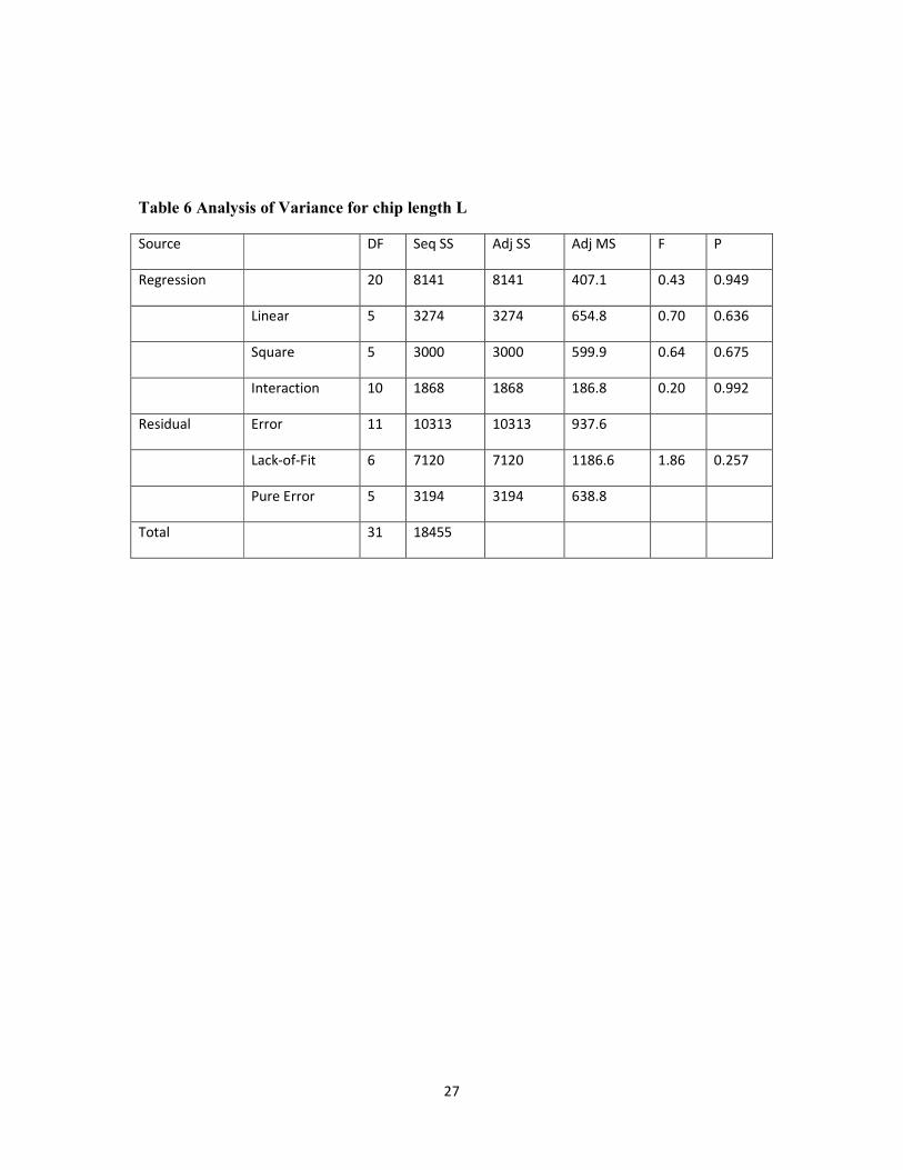
From table 6, analyzing of variance shows that the terms have values of probability more than

0.05 which make them insignificant. Since all the linear, square and interaction terms are

insignificant in this case, which is not possible. Hence, it concludes that error has crept into

the model and it requires repetition.

Table 7 of estimated regression coefficients using coded units show that almost all the factors

have a high probability value of being insignificant.

In table 8 of unusual observation of ξ, two values show a large standardized residual unusual

observation implying that the observations are not correct and are to be repeated.

In fig. 5.8, the histogram of residuals is shown that has a normal distribution with a few

observations deviating from the normal curve. If this assumption is valid, a histogram plot of

the residuals should look like a sample form a normal distribution.

In fig. 5.9, the graph of normal probability plot vs residuals shows that most of the

points are near the line implying the residual is normal. Observations showing standardized

residual greater than 2 and less than -2 are to be investigated and may be the experiments

repeated to get the adequate model.

In fig. 5.10, the graph of residuals vs fitted values, the values which are greater than 2

and less than -2 are insignificant

In fig. 5.11, we check the correlation between residuals by plotting residuals in

sequence and the graph of residual vs order of data shows the standardized residual for the

run order of experiment. This implies that the residuals are random in nature and don’t

exhibit any pattern with run order.

27

Table 6 Analysis of Variance for chip length L

Source DF Seq SS Adj SS Adj MS F P

Regression 20 8141 8141 407.1 0.43 0.949

Linear 5 3274 3274 654.8 0.70 0.636

Square 5 3000 3000 599.9 0.64 0.675

Interaction 10 1868 1868 186.8 0.20 0.992

Residual Error 11 10313 10313 937.6

Lack-of-Fit 6 7120 7120 1186.6 1.86 0.257

Pure Error 5 3194 3194 638.8

Total 31 18455

28

Table 7 Estimated Regression Coefficients for chip length (The analysis was done using

coded units.)

Term Coefficient SE Coefficient T P

Constant 42.9896 8.751 4.913 0.000

s 0.1276 7.217 0.018 0.986

f 9.4497 7.217 1.309 0.217

d 6.9274 7.217 0.960 0.358

H -2.4914 7.217 -0.345 0.736

W -6.1950 7.217 -0.858 0.409

s*s -1.0742 19.520 -0.055 0.957

f*f 9.0128 19.520 0.462 0.653

d*d -24.9582 19.520 -1.279 0.227

H*H -2.9642 19.520 -0.152 0.882

W*W 26.0388 19.520 1.334 0.209

s*f -0.2224 7.655 -0.029 0.977

s*d 0.0076 7.655 0.001 0.999

s*H -2.4852 7.655 -0.325 0.752

s*W -1.0111 7.655 -0.132 0.897

f*d -5.1058 7.655 -0.667 0.519

f*H -7.3683 7.655 -0.963 0.356

f*W 2.7861 7.655 0.364 0.723

d*H -3.6881 7.655 -0.482 0.639

d*W -2.7794 7.655 -0.363 0.723

H*W -0.2182 7.655 -0.029 0.978

S = 30.62 R-Sq = 44.1% R-Sq(adj) = 0.0%

29

Table 8 Unusual observation for chip length

Obs Std

Order

L Fit SE Fit Residual Std

Residual

remark

1 1 17.857 11.196 30.072 6.661 1.15

2 2 33.203 28.819 30.072 4.384 0.76

3 3 10.537 11.104 21.819 -0.567 -0.03

4 4 16.625 26.553 30.072 -9.928 -1.72

5 5 43.253 49.772 30.072 -6.519 -1.13

6 6 57.925 63.804 30.072 -5.879 -1.02

7 7 49.699 43.678 30.072 6.021 1.04

8 8 49.009 53.252 30.072 -4.243 -0.74

9 9 69.931 59.862 30.072 10.069 1.75

10 10 37.385 42.990 8.751 -5.605 -0.19

11 11 24.957 42.990 8.751 -18.033 -0.61

12 12 29.518 42.553 21.819 -13.035 -0.61

13 13 13.289 42.517 21.819 -29.228 -1.36

14 14 41.569 42.990 8.751 -1.421 -0.05

15 15 90.955 42.990 8.751 47.965 1.63

16 16 79.168 42.043 21.819 37.125 1.73

17 17 75.837 61.452 21.819 14.385 0.67

18 18 48.553 75.223 21.819 -26.670 -1.24

19 19 90.854 62.833 21.819 28.021 1.30

20 20 20.508 42.990 8.751 -22.482 -0.77

21 21 6.013 41.788 21.819 -35.775 -1.67

22 22 37.162 42.990 8.751 -5.828 -0.20

30

Obs Std

Order

L Fit SE Fit Residual Std

Residual

remark

23 23 68.112 37.534 21.819 30.578 1.42

24 24 69.429 66.506 30.072 2.923 0.51

25 25 37.966 40.728 30.072 -2.762 -0.48

26 26 26.876 24.959 21.819 1.917 0.09

27 27 71.314 58.128 30.072 13.186 2.29 R

28 28 42.851 43.977 30.072 -1.126 -0.20

29 29 57.019 54.736 30.072 2.283 0.40

30 30 60.277 63.679 30.072 -3.402 -0.59

31 31 83.889 83.243 30.072 0.646 0.11

32 32 23.112 36.778 30.072 -13.666 -2.37 R

R denotes an observation with a large standardized residual.

31

Fig 5.8 Histograms of the residuals for chip length

Fig 5.9 Normal probability plot of the residuals for chip length

32

Fig 5.10 Residuals vs the order of the data for chip length

Fig. 5.11 Residuals vs the fitted values for chip length

33

Table 9 Estimated Regression Coefficients for ξξξξ and chip length using data in uncoded

units

Term Coefficient for ξξξξ Coefficient for chip length

Constant 1.4852 254.318

s 0.1757 2.2692

f -1.3517 10.715

d -4.2948 558.025

H -2.6773 301.182

W -1.5065 -208.81

s*s -0.0022 -0.0107

f*f 2.0179 225.319

d*d 5.3929 -623.96

H*H 1.8097 -131.74

W*W 0.0957 26.0388

s*f 0.02 -0.1112

s*d -0.0506 0.0038

s*H 0.0408 -1.6568

s*W 0.0121 -0.1011

f*d -0.1875 -127.65

f*H -1.8333 -245.61

f*W 0.05 13.9303

d*H 0.0417 -122.94

d*W 0.4313 -13.897

H*W -0.075 -1.4546

34

Developed equation for ξ:

ξ = 1.4852 + 0.1757*s -1.3517*f -4.2948*d -2.6773*H -1.5065*W -0.0022*s*s +2.0179*f*f +

5.3929*d*d +1.8097*H*H + 0.0957*W*W + 0.02*s*f -0.0506*s*d + 0.0408*s*H + 0.0121*s*W -

0.1875*f*d -1.8333*f*H + 0.05*f*W + 0.0417*d*H + 0.4313*d*W -0.075*H*W

Developed equation for chip length:

Chip length= 254.318 +2.2692*s +10.715*f +558.025*d +301.182*H -208.81*W -0.0107*s*s

+225.319*f*f -623.96*d*d -131.74*H*H +26.0388*W*W -0.1112*s*f +0.0038*s*d -1.6568*s*H -

0.1011*s*W -127.65*f*d -245.61*f*H +13.9303*f*W -122.94*d*H -13.897*d*W -1.4546*H*W

35

CONCLUSION:

The effect of cutting speed, feed, depth of cut and chip breaker height and width on the chip

breakability was studied.

It was found that chips of greater thickness are produced at low feed and depth of cut

and it gradually decreases as feed and depth of cut increases.

Cutting speed and depth of cut are the most significant factors affecting the chip

breakability and even their higher order terms play a significant role. The graphs obtained

from histogram of residuals show a normal distribution. The graph of normal probability plot

vs residuals shows that most of the points are near the line implying the residual is normal.

Thus, it was concluded that speed and depth of cut are most important factors in

better control of chip.

36

REFERENCES:

[1] Kim J.D., Kweun O.B., A chip-breaking system for mild steel in turning, International

Journal of machine tools manufacture, vol.37, no.5, (1997), 607-617.

[2] Mesquita R.M.D, Soares F.A.M., Barata Marques M.J.M., An experimental study of the

effect of cutting speed on chip breaking, Journal of Materials Processing Technology, 56

(1996) 313-320.

[3] Hong-Gyoo Kim, Jae-Hyung Sim, Hyeog-Jun Kweon, Performance evaluation of chip

breaker utilizing neural network, Journal of materials processing technology 2 0 9 ( 2 0 0 9 )

647–656

[4] Das N.S., Chawla B.S., Biswas C.K., An analysis of strain in chip breaking using slip-line

field theory with adhesion friction at chip/tool interface, Journal of Materials Processing

Technology 170 (2005), 509–515

[5] Maity K.P., Das N.S., A slip-line solution to metal machining using a cutting tool with a

step-type chip-breaker, Journal of Materials Processing Technology, 79, ( 1998), 217-223

[6] Rahman M., Seah K.W.H., Li X.P. and Zhang X.D.,A three-dimensional model of chip

flow, chip curl and chip breaking under the concept of equivalent parameters, Int. J. Mach.

Tools Manufacture., Vol. 35, (1995) pp. 1015-1031.

[7] Sutter G., Chip geometries during high-speed machining for orthogonal cutting

conditions, International Journal of Machine Tools & Manufacture 45 (2005) 719–726

[8] Komanduri R., Schroeder T., Hazra J., Turkovich B.F. von, Flom D.G., On the

catastrophic shear instability in high-speed machining of an AISI 4340 steel, Journal of

Engineering for Industry,104, (1982) 121–131

[9] Friedman M.Y., Lenz E., Investigation of tool-chip contact length in metal cutting,

International Journal of Machine Tool Design and Research ,10 (1970) 401–416.

[10] Sutter G., Molinari G., Faure L., Klepaczko J.R., Dudzinski D., An experimental study

of high speed orthogonal cutting, Transactions ASME, Journal of Manufacturing Science and

Engineering ,12 (1998) 169–172.

37

[11] Dabade Uday A., Joshi Suhas S., Analysis of chip formation mechanism in machining

of Al/SiCp metal matrix composites, Journal of Materials Process. Tech. (2009)

[12] B.L. Juneja, G.S. Sekhon, Fundamentals of metal cutting and machine tools, Wiley

Eastern, New Delhi, India, 1987.

[13] T. Shi, S. Ramalingam, Slip-line solution for orthogonal cutting with a chip breaker and

flank wear, International Journal Mechanical Science, 33 (9) (1991) 689–774.

[14] B. Worthington and M. H. Rahman, Predicting breaking with groove type breakers,

International Journal Mach. Tool Design Research,. 19, 121-132 (1979).