Evaluation of Advanced Lukas-Kanade Optical Flowon Thoracic 4D-CT

Christoph Bernhard Hoog Antink ·Tarunraj Singh · Puneet Singla ·Matthew Podgorsak

Received: March 2002 / Accepted: April 2003

Abstract Extensive use of high frequency imaging in medical applicationspermit the estimation of velocity fields which corresponds to motion of land-marks in the imaging field. The focus of this work is on the development ofa robust local optical flow algorithm for velocity field estimation in medicalapplications. Local polynomial fits to the medical image intensity-maps areused to generate convolution operators to estimate the spatial gradients. Anovel polynomial window function with a compact support is used to differ-entially weight the optical flow gradient constraints in the region of interest.Tikhonov regularization is exploited to synthesize a well posed optimizationproblem and to penalize large displacements. The proposed algorithm is testedand validated on benchmark datasets for deformable image registration. Theten datasets include large and small deformations, and illustrate that the pro-posed algorithm outperforms or is competitive with other algorithms testedon this dataset, when using mean and variance of the displacement error asperformance metrics.

Keywords Optical Flow · Acute Illness · Deformable Image Registration ·Radiotherapy Planning

The authors would like to thank the National Science Foundation, which funded this projectunder grant CMMI-#0928630. C. Hoog Antink also would like to thank Fulbright and theGerman National Academic Foundation for partial funding.

Christoph Bernhard Hoog AntinkDept. of Mechanical and Aerospace EngineeringSUNY at BuffaloBuffalo, NY 14260USAE-mail: choogant@buffalo.edu

2 Christoph Bernhard Hoog Antink et al.

1 Introduction

Optical flow for estimating velocity fields has numerous applications in themedical field. In Interstitial Laser Therapy (ILT), thermal energy is depositedvia lasers to treat tumors which are accessible via needle insertion. Magneticresonance imaging (MRI) provides the ability to locate the target, guide theoptical fiber and monitor the thermal effects [17]. This especially reduces in-vasiveness of the procedure by making implanted thermic sensors obsolete.At the same time, spatiotemporal information of the thermal effects can beobtained and analyzed using optical flow.

In applications such as TAVI (Transcatheter Aortic Valve Implantation)where a vioprosthetic aortic valve is implanted to replace a severly stenoticaortic valve, echocardiography and fluoroscopy play an important role today.Optical flow can be used in this acute illness application for the estimationof velocity field to assist placement of the guidewire and valve positioning [9].In addition, when thinking about future applications such as active roboticsurgical devices, it is obvious that highly accurate motion information thatcan be computed in real-time is crucial. Optical flow provides a method toobtain these from imaging modalities that are already in use.

One of the most important factors in successful acute illness interventionsuch as TAVI is patient diagnosis and planning of the procedure. Four Dimen-sional Ultrasound provides an excellent non-invasive source of dynamic cardiacinformation. However, the analysis of this data can be time-consuming and isprone to human error. Optical flow can be used to assist in the derivation ofqualitative and quantitative cardiac information such as Left Ventricular LongAxis over time [15,8] that could be used for patient selection, therapy plan-ning and follow-up. With a high accuracy, real-time method, more complexparameters like stroke volume could be monitored non-invasively.

Deformable Image Registration (DIR) of Computed Tomography (CT)scans for radiotherapy planning is another area where optical flow has provento be an invaluable tool [16,10]. Here, large deformations in the range of 4cmand artifacts in the image data pose challenges on the estimator. At the sametime, high demands are put on the accuracy of the algorithm, since small er-rors in the estimated velocity fields can finally lead to severe over irradiating ofhealthy tissue when used to create faulty therapy plans. For the application ofoptical flow as DIR, an elaborate benchmark problem [4,2] exists, which willbe used in this work. Other objective benchmark problems exist, the interestedreader may find an extensive set of tests and state-of-the-art algorithms in the”EMPIRE10 Challenge” [13].

The main focus of this paper is to create an efficient optical flow algorithmthat has the accuracy and robustness necessary for medical applications. Forthis we propose an optical flow algorithm based on the Lucas/Kanade al-gorithm, which is a local method [12]. Several improvements to the originalalgorithms are made which are described in the paper.

Evaluation of Advanced Lukas-Kanade Optical Flow on Thoracic 4D-CT 3

– Robust gradient calculation:Early optical flow algorithms used finite difference to determine the spatialand time gradients. Since smoothness assumptions are integral to opticalflow algorithms, a local polynomial fit to the intensity variations about thepixel of interest is synthesized. The determination of the spatial gradientcan now can carried out easily.

– Non-Gaussian weighting function:The Lucas-Kanada algorithm uses a small spatial neighborhood of the pixelof interest to determine the local flow field. A weighting function is usedto give more importance to the constraint at the center of the local patchrelative to the pixels at the periphery. A recently developed finite supportfunction where the desired smoothness can be prescribed is used to weightthe pixel in the local patch.

– Tikhonov Regularization: For least squares problem which are ill posed,preference is given to solution with specific properties such as ones withsmall norm of the solution vector, smooth solution. This can be achievedvia Tikhonov regularization which corresponds to including an additionalterm to the cost function. The optical flow problem is ill-posed and to favorsmall velocity field, Tikhonov regularization is achieved by penalizing thenorm of the velocity field.

– Balanced Optical Flow: There is a desire to minimize the inconsistency inthe velocity field when going from image 1 to image 2 and from image 2to image 1. To achieve this goal, a simple technique which determines thetwo velocity fields, inverts the second, interpolates it to match the originalgrid and averaged is proposed in this work.

The resulting algorithm is implemented in MATLAB / C and applied to a setof benchmark problems [4,2]. In contrast to other non-quadratic optical flowformulations, the algorithm does not rely on a complex and potentially com-putational expensive minimization step but on well-posed matrix inversions.

The paper is outlined as follows: Section 2 describes the mathematicaland algorithmic details of the proposed algorithm. Section 3 gives a detaileddescription of the benchmark data used to evaluate the performance of theproposed algorithm. Section 4 presents the results, which are then discussedin Section 5. In Section 6 conclusions are drawn and future work is proposed.

2 Methods

2.1 Optical Flow

Optical flow methods calculate an approximation of the motion field from time-varying image intensities. A common assumption in optical flow methods isthat voxel intensities I might translate from one frame to another but theirintensities are constant [11]. If we assume this translations to be small theycan be well approximated by the Taylor series expansion [12]. This leads to

4 Christoph Bernhard Hoog Antink et al.

the gradient constraint equation:

0 = u(x, y, z, t)Ix + v(x, y, z, t)Iy + w(x, y, z, t)Iz + It (1)

Ix =∂

∂xI (x, y, z, t) , Iy =

∂

∂yI (x, y, z, t) , Iz =

∂

∂zI (x, y, z, t) ,

It =∂

∂tI (x, y, z, t)

where u(x, y, z, t), v(x, y, z, t) and w(x, y, z, t) refer to the normalized velocitycomponents in the x, y, z directions at time t.

2.1.1 Gradient Calculation

For the sake of clarity, the calculation of image gradients is delineated for two-dimensional images, the three-dimensional implementation is a straightforwardextension. In digital image processing applications, images are represented dis-cretely both in space and amplitude (grey-value). Spatial gradients are obtainby convolving the image with a filter kernel hp as given in the equation:

∂

∂pI (x, y, t) =

k=∞∑k=−∞

l=∞∑l=−∞

I (k, l)hp (x− k, y − l) = I (x, y, t) ∗ hp (2)

To increase robustness of the gradient calculation, the intensity distributionI (x, y, t) will be approximated locally (IL) by a polynomial function, in thisexample a cubic:

IL (x, y, t) = a1 + a2x+ a3y + a4x2 + a5y

2 + (3)

a6xy + a7xy2 + a8yx

2 + a9x3 + a10y

3

Considering a patch of n by m pixels, this can be rewritten in matrix notation:

IL = Ma (4)

M =

1 x1 y1 x21 y21 x1y1 x1y

21 y1x

21 x31 y31

1 x2 y2 x22 y22 x2y2 x2y22 y2x

22 x32 y32

...1 xnm ynm x2nm y2nm xnmynm xnmy

2nm ynmx

2nm x3nm y3nm

(5)

a = [a1 a2 a3 a4 a5 a6 a7 a8 a9 a10]′

(6)

Here, the number of rows in the matrix M corresponds to the number of pixelsin the patch. If we select a patch IL of 5x5 pixels, the system is overdeterminedand can be solved in the least-squares sense:

a = (M ′wM)−1M ′w · IL = W · IL (7)

Here, w is a diagonal weighting matrix that can be used to give more weight onthe central pixels. For example, a Gaussian weighting function could be used.In our approach, however, we use a novel polynomial weighting function [14].

Evaluation of Advanced Lukas-Kanade Optical Flow on Thoracic 4D-CT 5

This function gracefully ranges from zero to one over the compact support,unlike a Gaussian with infinite tails.

Examining Equation 7 makes obvious the fact that the matrix inversionhas to be computed only once, after which the parameters can be obtainedby a simple multiplication of the matrix W with the patch IL. Note that thisapproach also makes prior image-smoothing obsolete. If we now define thecentral pixel of our patch to have the coordinates x = 0, y = 0, the gradientsat this point are given by

∂

∂xIL (0, 0, t) = a2,

∂

∂yIL (0, 0, t) = a3 (8)

So, only the second and third row of the matrix W are of interest. If we rear-range them into a two-dimensional 5x5 array, the calculation of the gradientcan again be calculated by a two-dimensional convolution with the filter kernelgiven by Equation 9 :

hx =

W (2, 1) W (2, 2) W (2, 3) W (2, 4) W (2, 5)W (2, 6) W (2, 7) W (2, 8) W (2, 9) W (2, 10)W (2, 11) W (2, 12) W (2, 13) W (2, 14) W (2, 15)W (2, 16) W (2, 17) W (2, 18) W (2, 19) W (2, 20)W (2, 21) W (2, 22) W (2, 23) W (2, 24) W (2, 25)

= hy′ (9)

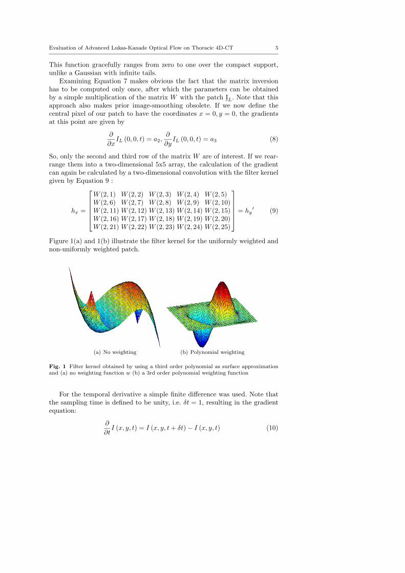
Figure 1(a) and 1(b) illustrate the filter kernel for the uniformly weighted andnon-uniformly weighted patch.

(a) No weighting (b) Polynomial weighting

Fig. 1 Filter kernel obtained by using a third order polynomial as surface approximationand (a) no weighting function w (b) a 3rd order polynomial weighting function

For the temporal derivative a simple finite difference was used. Note thatthe sampling time is defined to be unity, i.e. δt = 1, resulting in the gradientequation:

∂

∂tI (x, y, t) = I (x, y, t+ δt)− I (x, y, t) (10)

6 Christoph Bernhard Hoog Antink et al.

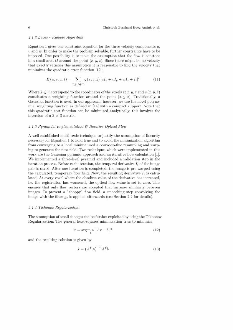
2.1.2 Lucas - Kanade Algorithm

Equation 1 gives one constraint equation for the three velocity components u,v and w. In order to make the problem solvable, further constraints have to beimposed. One possibility is to make the assumption that the flow is constantin a small area Ω around the point (x, y, z). Since there might be no velocitythat exactly satisfies this assumption it is reasonable to find the velocity thatminimizes the quadratic error function [12]:

E (u, v, w, t) =∑

x,y,z∈Ωg (x, y, z) [uIx + vIy + wIz + It]

2(11)

Where x, y, z correspond to the coordinates of the voxels at x, y, z and g (x, y, z)constitutes a weighting function around the point (x, y, z). Traditionally, aGaussian function is used. In our approach, however, we use the novel polyno-mial weighting function as defined in [14] with a compact support. Note thatthis quadratic cost function can be minimized analytically, this involves theinversion of a 3 × 3 matrix.

2.1.3 Pyramidal Implementation & Iterative Optical Flow

A well established multi-scale technique to justify the assumption of linearitynecessary for Equation 1 to hold true and to avoid the minimization algorithmfrom converging to a local minima used a coarse-to-fine resampling and warp-ing to generate the flow field. Two techniques which were implemented in thiswork are the Gaussian pyramid approach and an iterative flow calculation [1].We implemented a three-level pyramid and included a validation step in theiteration process. Before each iteration, the temporal derivative It of the imagepair is saved. After one iteration is completed, the image is pre-warped usingthe calculated, temporary flow field. Now, the resulting derivative It is calcu-lated. At every voxel where the absolute value of the derivative has increased,i.e. the registration has worsened, the optical flow value is set to zero. Thisensures that only flow vectors are accepted that increase similarity betweenimages. To prevent a ”choppy” flow field, a smoothing step convolving theimage with the filter gs is applied afterwards (see Section 2.2 for details).

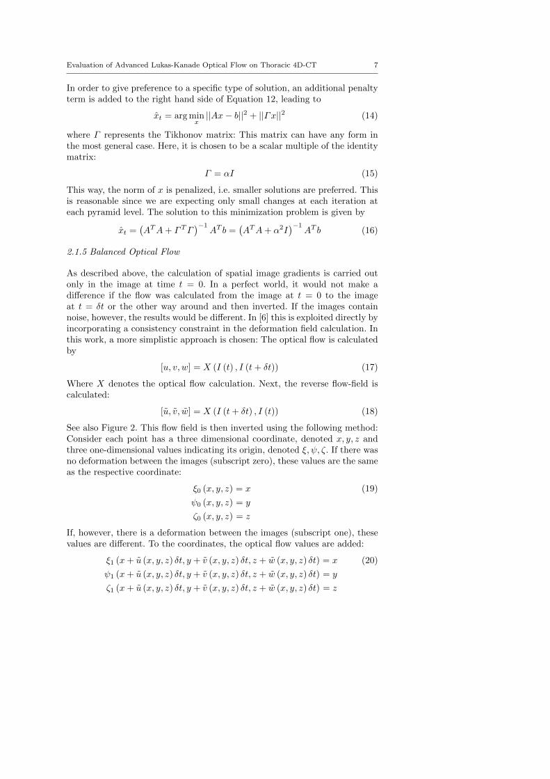
2.1.4 Tikhonov Regularization

The assumption of small changes can be further exploited by using the TikhonovRegularization: The general least-squares minimization tries to minimize

x = arg minx||Ax− b||2 (12)

and the resulting solution is given by

x =(ATA

)−1AT b (13)

Evaluation of Advanced Lukas-Kanade Optical Flow on Thoracic 4D-CT 7

In order to give preference to a specific type of solution, an additional penaltyterm is added to the right hand side of Equation 12, leading to

xt = arg minx||Ax− b||2 + ||Γx||2 (14)

where Γ represents the Tikhonov matrix: This matrix can have any form inthe most general case. Here, it is chosen to be a scalar multiple of the identitymatrix:

Γ = αI (15)

This way, the norm of x is penalized, i.e. smaller solutions are preferred. Thisis reasonable since we are expecting only small changes at each iteration ateach pyramid level. The solution to this minimization problem is given by

xt =(ATA+ ΓTΓ

)−1AT b =

(ATA+ α2I

)−1AT b (16)

2.1.5 Balanced Optical Flow

As described above, the calculation of spatial image gradients is carried outonly in the image at time t = 0. In a perfect world, it would not make adifference if the flow was calculated from the image at t = 0 to the imageat t = δt or the other way around and then inverted. If the images containnoise, however, the results would be different. In [6] this is exploited directly byincorporating a consistency constraint in the deformation field calculation. Inthis work, a more simplistic approach is chosen: The optical flow is calculatedby

[u, v, w] = X (I (t) , I (t+ δt)) (17)

Where X denotes the optical flow calculation. Next, the reverse flow-field iscalculated:

[u, v, w] = X (I (t+ δt) , I (t)) (18)

See also Figure 2. This flow field is then inverted using the following method:Consider each point has a three dimensional coordinate, denoted x, y, z andthree one-dimensional values indicating its origin, denoted ξ, ψ, ζ. If there wasno deformation between the images (subscript zero), these values are the sameas the respective coordinate:

ξ0 (x, y, z) = x (19)

ψ0 (x, y, z) = y

ζ0 (x, y, z) = z

If, however, there is a deformation between the images (subscript one), thesevalues are different. To the coordinates, the optical flow values are added:

ξ1 (x+ u (x, y, z) δt, y + v (x, y, z) δt, z + w (x, y, z) δt) = x (20)

ψ1 (x+ u (x, y, z) δt, y + v (x, y, z) δt, z + w (x, y, z) δt) = y

ζ1 (x+ u (x, y, z) δt, y + v (x, y, z) δt, z + w (x, y, z) δt) = z

8 Christoph Bernhard Hoog Antink et al.

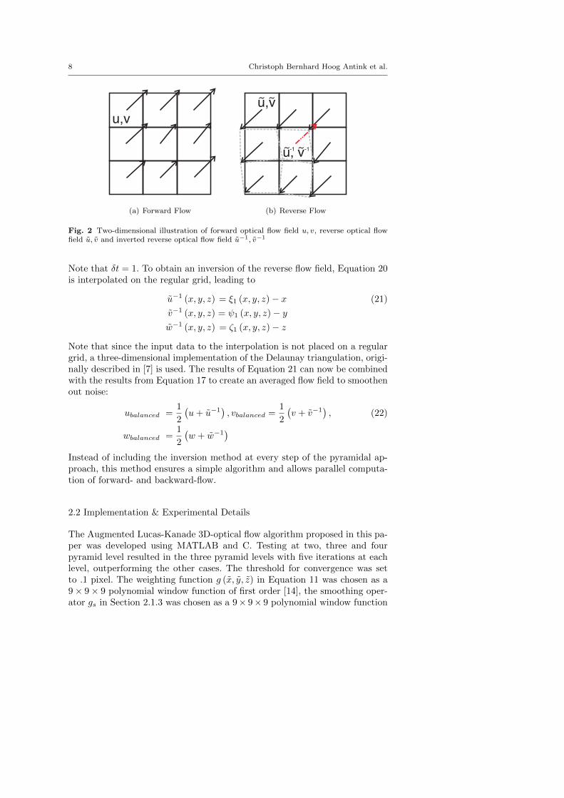
(a) Forward Flow (b) Reverse Flow

Fig. 2 Two-dimensional illustration of forward optical flow field u, v, reverse optical flowfield u, v and inverted reverse optical flow field u−1, v−1

Note that δt = 1. To obtain an inversion of the reverse flow field, Equation 20is interpolated on the regular grid, leading to

u−1 (x, y, z) = ξ1 (x, y, z)− x (21)

v−1 (x, y, z) = ψ1 (x, y, z)− yw−1 (x, y, z) = ζ1 (x, y, z)− z

Note that since the input data to the interpolation is not placed on a regulargrid, a three-dimensional implementation of the Delaunay triangulation, origi-nally described in [7] is used. The results of Equation 21 can now be combinedwith the results from Equation 17 to create an averaged flow field to smoothenout noise:

ubalanced =1

2

(u+ u−1

), vbalanced =

1

2

(v + v−1

), (22)

wbalanced =1

2

(w + w−1

)Instead of including the inversion method at every step of the pyramidal ap-proach, this method ensures a simple algorithm and allows parallel computa-tion of forward- and backward-flow.

2.2 Implementation & Experimental Details

The Augmented Lucas-Kanade 3D-optical flow algorithm proposed in this pa-per was developed using MATLAB and C. Testing at two, three and fourpyramid level resulted in the three pyramid levels with five iterations at eachlevel, outperforming the other cases. The threshold for convergence was setto .1 pixel. The weighting function g (x, y, z) in Equation 11 was chosen as a9× 9× 9 polynomial window function of first order [14], the smoothing oper-ator gs in Section 2.1.3 was chosen as a 9× 9× 9 polynomial window function

Evaluation of Advanced Lukas-Kanade Optical Flow on Thoracic 4D-CT 9

of third order. The polynomial derivative kernels hp to acquire Ix, Iy, Iz, seeEquation 1 and 2, was set to be of size 5 × 5 × 5 (the patch size) using athird order polynomial. The weighting function w mentioned in Equation 7was decided to be a polynomial windowing function of order 20. All convolu-tion operations were preceded by a border padding operation mirroring thedata at its borders. The regularization term α (see Equation 15 ) was cho-sen to be 100. All parameters were tuned using 300 landmark pairs per caseprovided for download at http://www.dir-lab.com. Note that the parametersof the algorithm were constant for all cases, no case-to-case tuning was per-formed. The calculations were performed on the Xeon X5460-server (32GBRAM, 8 x Intel(R) @ 3.16GHz with four cores each). For the first five cases,it took approximately 13 minutes per phase (i.e. T00% → T10%) for theoptical flow calculations and approximately 55 minutes for the optical flowand inversion calculations (i.e. (T10%→ T00%)

−1). For case six to ten, a

coarse region-of-interest of 300 × 412 x Z voxels was selected, where Z cor-responds to the number of voxels in z− direction for the corresponding case.This bounding box was identical for all cases and data outside the ribcage thatcontained no useful information was cut out. This helped to reduce the datato be processed by a factor of approximately 2. After this, the correspondingcomputation times were approximately 40 / 73 minutes for case six to ten.The execution time of the loop processing Equation 16 could be reduced by afactor of approximately 70 by writing this function in C, this reduced the over-all optical flow calculation time by a factor of 2. Note that every calculationused only one processor core at a time. To increase overall speed, up to tenoptical flow calculations could be run in parallel. The bottleneck turned outto be the RAM since the inversion of the optical flow field using Delaunay Tri-angulation in the form of MATLAB’s TriScatteredInterp function consumedtremendous amounts of memory. To improve this, the implementation of anapproach like the one described in [5] can be used. For each case, a total ofsix CT images was processed, with T00% corresponding to the extreme inhaleand T50% corresponding to the extreme exhale phase. The total deformationfield T00%→ T50% was obtained by sequentially synthesizing each phase-to-phase deformation field (T00%→ T10%, T10%→ T20%, ..., T40%→ T50%).The resulting displacement fields were sent to The University of Texas M DAnderson Cancer Center for evaluation1.

3 Benchmark Data

Castillo et. al. published a paper [4] on the objective evaluation of DIR algo-rithms using a large dataset of expert determined landmarks: For their frame-work, they used five sets of thoracic 4DCT images that were acquired frompatients undergoing treatment in their facility. The images were cropped andresampled in the xy plane (transversal plane) to contain the full rib cage at

1 The author would like to acknowledge the help of Richard Castillo, MS who processedthe result of our algorithm and provided feedback regarding its performance.

10 Christoph Bernhard Hoog Antink et al.

a resolution of 256 × 256 pixels. No alteration was done in the z−direction(Superior-Inferior (SI) direction). This leads to different voxel sizes and imagedimensions. Using this data they manually identified more than 1100 land-mark pairs in the extreme inhale (T00%) and extreme exhale (T50%) imageof every set. This process was done by the primary reader, an ”expert in tho-racic imaging” using a software developed for this purpose. From these points,a subset of 200 points was randomly selected and re-registered by the primaryreader to determine the intra-observer error. The same set of points was thenre-registered by two secondary readers to quantify the inter-observer error.They then implemented two different DIR algorithms and performed a statis-tical analysis that showed that ”large sets” of landmarks are indeed necessaryto evaluate DIR accuracy with a certain accuracy. For these test cases andthe optical flow algorithm they implemented, they find that 1000 pairs arenecessary to evaluate the accuracy with 95% confidence.

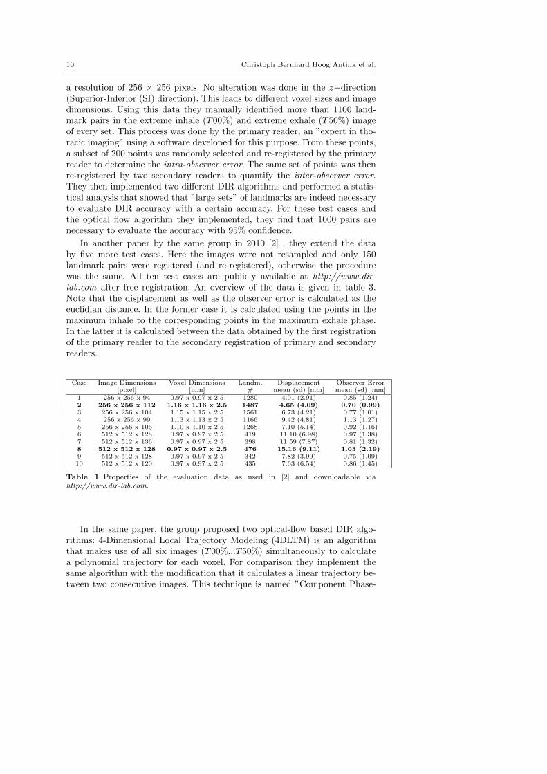
In another paper by the same group in 2010 [2] , they extend the databy five more test cases. Here the images were not resampled and only 150landmark pairs were registered (and re-registered), otherwise the procedurewas the same. All ten test cases are publicly available at http://www.dir-lab.com after free registration. An overview of the data is given in table 3.Note that the displacement as well as the observer error is calculated as theeuclidian distance. In the former case it is calculated using the points in themaximum inhale to the corresponding points in the maximum exhale phase.In the latter it is calculated between the data obtained by the first registrationof the primary reader to the secondary registration of primary and secondaryreaders.

Case Image Dimensions Voxel Dimensions Landm. Displacement Observer Error[pixel] [mm] # mean (sd) [mm] mean (sd) [mm]

1 256 x 256 x 94 0.97 x 0.97 x 2.5 1280 4.01 (2.91) 0.85 (1.24)2 256 x 256 x 112 1.16 x 1.16 x 2.5 1487 4.65 (4.09) 0.70 (0.99)3 256 x 256 x 104 1.15 x 1.15 x 2.5 1561 6.73 (4.21) 0.77 (1.01)4 256 x 256 x 99 1.13 x 1.13 x 2.5 1166 9.42 (4.81) 1.13 (1.27)5 256 x 256 x 106 1.10 x 1.10 x 2.5 1268 7.10 (5.14) 0.92 (1.16)6 512 x 512 x 128 0.97 x 0.97 x 2.5 419 11.10 (6.98) 0.97 (1.38)7 512 x 512 x 136 0.97 x 0.97 x 2.5 398 11.59 (7.87) 0.81 (1.32)8 512 x 512 x 128 0.97 x 0.97 x 2.5 476 15.16 (9.11) 1.03 (2.19)9 512 x 512 x 128 0.97 x 0.97 x 2.5 342 7.82 (3.99) 0.75 (1.09)10 512 x 512 x 120 0.97 x 0.97 x 2.5 435 7.63 (6.54) 0.86 (1.45)

Table 1 Properties of the evaluation data as used in [2] and downloadable viahttp://www.dir-lab.com.

In the same paper, the group proposed two optical-flow based DIR algo-rithms: 4-Dimensional Local Trajectory Modeling (4DLTM) is an algorithmthat makes use of all six images (T00%...T50%) simultaneously to calculatea polynomial trajectory for each voxel. For comparison they implement thesame algorithm with the modification that it calculates a linear trajectory be-tween two consecutive images. This technique is named ”Component Phase-

Evaluation of Advanced Lukas-Kanade Optical Flow on Thoracic 4D-CT 11

to-Phase” (CPP) by the group. They show a clear advantage of 4DLTM overCPP in mean and standard deviation of 3D Euclidian error.

More algorithms were implemented by the same group in [3] and [10], theresults are also available on-line and proved the superior accuracy of 4DLTM.

4 Results

Figures 3 and 4 illustrate the results for case 2 and 8 in comparison to otheralgorithms in terms of mean and standard deviation of the euclidian registra-tion error as published in [4,2,3,10] and listed on http://www.dir-lab.com (asof 06/13/2012). The vertical bars include a marker which corresponds to themean of the error and the length of the bar is proportional to the varianceof the error. The magenta bar (leftmost bar) illustrates the error statistics ofthe human observer and the rest of the bars correspond to various algorithmsused to estimate the motion of the landmarks. The black bar immediately tothe right of the human observer statistics correspond to the results of the al-gorithm proposed in this paper. It is clear that for both cases (2 and 8), thealgorithm presented in the paper outperform all the algorithms tested by sci-entists at MD. Anderson who manage the datasets and postprocess the results.Figure 5 and 6 shows the manually obtained displacement field and the errorvector fields defined as pointing from the manually defined target location tothe predicted location using our DIR-algorithm. These cases were chosen to

0

0.5

1

1.5

2

2.5

3

3.5

err

or

in m

m

Evaluation Case #2

ALK

4DLTM2

CPP2

MLS1

CCLG3

COF3

LCI3

LII3

PF4

EPF4

AF4

DF4

ADF4

IC4

Human Observer

Fig. 3 Mean and standard deviation of the proposed optical flow algorithm in comparison toother algorithms for case 2: 1described in [4], 2described in [2], 3described in [3], 4describedin [10]

illustrate the performance of ALK for small (case 2) as well as large deforma-tions (case 8). The numerical results suggest that ALK has the capability ofaccurately registering 4DCT data, see Table 2.

It outperforms the CPP and 4DLTM approach presented in [2], althoughthe differences to the latter are small: Evaluating all landmark pairs of all tencases, the mean error of registration was determined to be 1.23 mm (with a

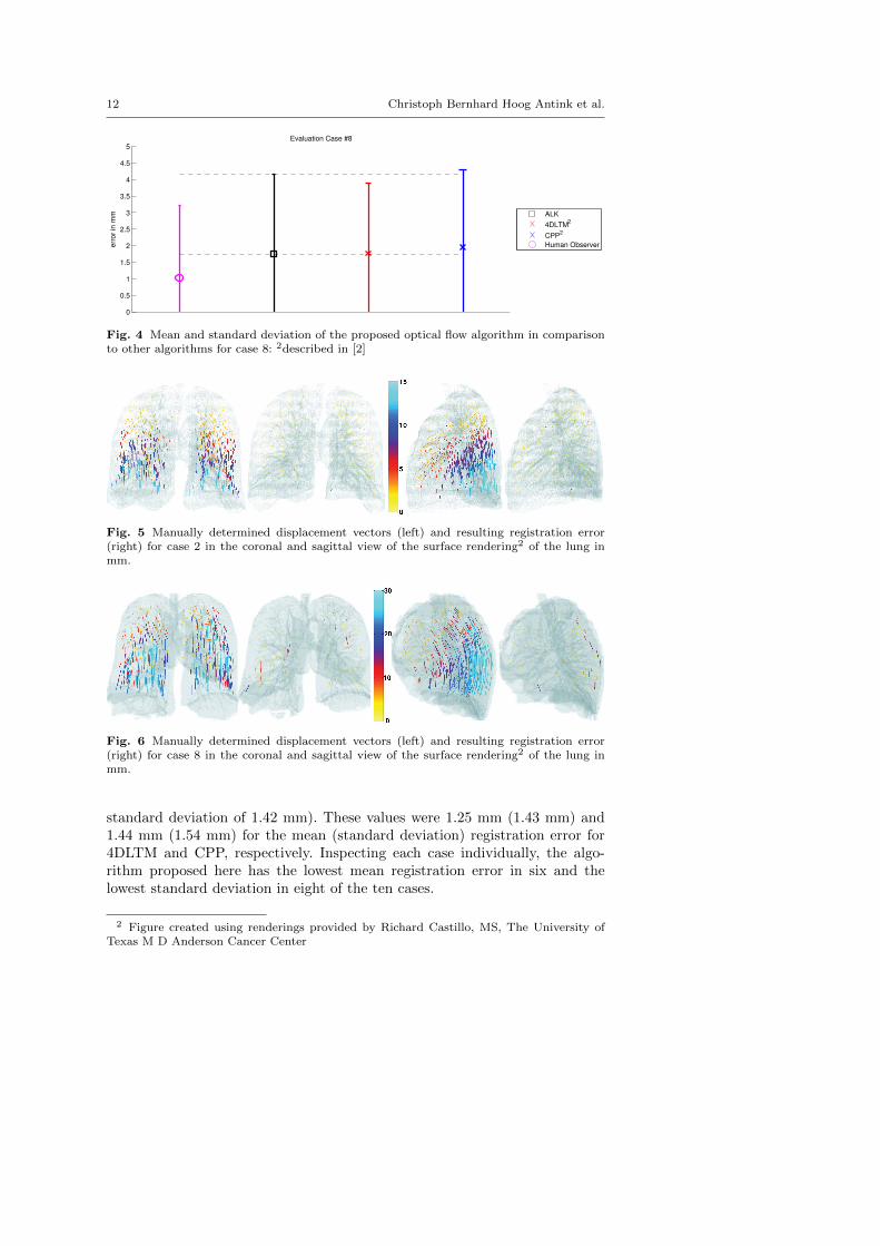
12 Christoph Bernhard Hoog Antink et al.

0

0.5

1

1.5

2

2.5

3

3.5

4

4.5

5

err

or

in m

m

Evaluation Case #8

ALK

4DLTM2

CPP2

Human Observer

Fig. 4 Mean and standard deviation of the proposed optical flow algorithm in comparisonto other algorithms for case 8: 2described in [2]

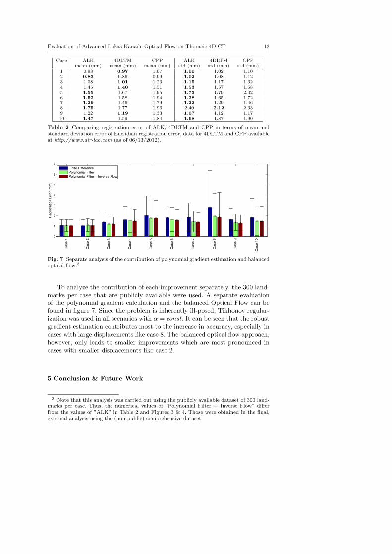
Fig. 5 Manually determined displacement vectors (left) and resulting registration error(right) for case 2 in the coronal and sagittal view of the surface rendering2 of the lung inmm.

Fig. 6 Manually determined displacement vectors (left) and resulting registration error(right) for case 8 in the coronal and sagittal view of the surface rendering2 of the lung inmm.

standard deviation of 1.42 mm). These values were 1.25 mm (1.43 mm) and1.44 mm (1.54 mm) for the mean (standard deviation) registration error for4DLTM and CPP, respectively. Inspecting each case individually, the algo-rithm proposed here has the lowest mean registration error in six and thelowest standard deviation in eight of the ten cases.

2 Figure created using renderings provided by Richard Castillo, MS, The University ofTexas M D Anderson Cancer Center

Evaluation of Advanced Lukas-Kanade Optical Flow on Thoracic 4D-CT 13

Case ALK 4DLTM CPP ALK 4DLTM CPPmean (mm) mean (mm) mean (mm) std (mm) std (mm) std (mm)

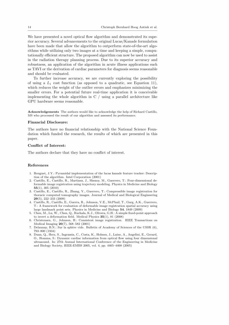
1 0.98 0.97 1.07 1.00 1.02 1.102 0.83 0.86 0.99 1.02 1.08 1.123 1.08 1.01 1.23 1.15 1.17 1.324 1.45 1.40 1.51 1.53 1.57 1.585 1.55 1.67 1.95 1.73 1.79 2.026 1.52 1.58 1.94 1.28 1.65 1.727 1.29 1.46 1.79 1.22 1.29 1.468 1.75 1.77 1.96 2.40 2.12 2.339 1.22 1.19 1.33 1.07 1.12 1.1710 1.47 1.59 1.84 1.68 1.87 1.90

Table 2 Comparing registration error of ALK, 4DLTM and CPP in terms of mean andstandard deviation error of Euclidian registration error, data for 4DLTM and CPP availableat http://www.dir-lab.com (as of 06/13/2012).

0

1

2

3

4

5

6

7

Regis

tration E

rror

[mm

]

Case 1

Case 2

Case 3

Case 4

Case 5

Case 6

Case 7

Case 8

Case 9

Case 1

0

Finite Difference

Polynomial Filter

Polynomial Filter + Inverse Flow

Fig. 7 Separate analysis of the contribution of polynomial gradient estimation and balancedoptical flow.3

To analyze the contribution of each improvement separately, the 300 land-marks per case that are publicly available were used. A separate evaluationof the polynomial gradient calculation and the balanced Optical Flow can befound in figure 7. Since the problem is inherently ill-posed, Tikhonov regular-ization was used in all scenarios with α = const. It can be seen that the robustgradient estimation contributes most to the increase in accuracy, especially incases with large displacements like case 8. The balanced optical flow approach,however, only leads to smaller improvements which are most pronounced incases with smaller displacements like case 2.

5 Conclusion & Future Work

3 Note that this analysis was carried out using the publicly available dataset of 300 land-marks per case. Thus, the numerical values of ”Polynomial Filter + Inverse Flow” differfrom the values of ”ALK” in Table 2 and Figures 3 & 4. Those were obtained in the final,external analysis using the (non-public) comprehensive dataset.

14 Christoph Bernhard Hoog Antink et al.

We have presented a novel optical flow algorithm and demonstrated its supe-rior accuracy. Several advancements to the original Lucas/Kanade formulationhave been made that allow the algorithm to outperform state-of-the-art algo-rithms while utilizing only two images at a time and keeping a simple, compu-tationally efficient structure. The proposed algorithm can now be used to assistin the radiation therapy planning process. Due to its superior accuracy androbustness, an application of the algorithm in acute illness applications suchas TAVI or the derivation of cardiac parameters for diagnosis seems reasonableand should be evaluated.

To further increase accuracy, we are currently exploring the possibilityof using a L1 cost function (as opposed to a quadratic, see Equation 11),which reduces the weight of the outlier errors and emphasizes minimizing thesmaller errors. For a potential future real-time application it is conceivableimplementing the whole algorithm in C / using a parallel architecture likeGPU hardware seems reasonable.

Acknowledgements The authors would like to acknowledge the help of Richard Castillo,MS who processed the result of our algorithm and assessed its performance.

Financial Disclosure:

The authors have no financial relationship with the National Science Foun-dation which funded the research, the results of which are presented in thispaper.

Conflict of Interest:

The authors declare that they have no conflict of interest.

References

1. Bouguet, J.Y.: Pyramidal implementation of the lucas kanade feature tracker: Descrip-tion of the algorithm. Intel Corporation (2001)

2. Castillo, E., Castillo, R., Martinez, J., Shenoy, M., Guerrero, T.: Four-dimensional de-formable image registration using trajectory modeling. Physics in Medicine and Biology55(1), 305 (2010)

3. Castillo, E., Castillo, R., Zhang, Y., Guerrero, T.: Compressible image registration forthoracic computed tomography images. Journal of Medical and Biological Engineering29(5), 222–233 (2009)

4. Castillo, R., Castillo, E., Guerra, R., Johnson, V.E., McPhail, T., Garg, A.K., Guerrero,T.: A framework for evaluation of deformable image registration spatial accuracy usinglarge landmark point sets. Physics in Medicine and Biology 54, 1849 (2009)

5. Chen, M., Lu, W., Chen, Q., Ruchala, K.J., Olivera, G.H.: A simple fixed-point approachto invert a deformation field. Medical Physics 35(1), 81 (2008)

6. Christensen, G., Johnson, H.: Consistent image registration. IEEE Transactions onMedical Imaging 20(7), 568–582 (2001)

7. Delaunay, B.N.: Sur la sphere vide. Bulletin of Academy of Sciences of the USSR (6),793–800 (1934)

8. Duan, Q., Herz, S., Ingrassia, C., Costa, K., Holmes, J., Laine, A., Angelini, E., Gerard,O., Homma, S.: Dynamic cardiac information from optical flow using four dimensionalultrasound. In: 27th Annual International Conference of the Engineering in Medicineand Biology Society, IEEE-EMBS 2005, vol. 4, pp. 4465–4468 (2005)

Evaluation of Advanced Lukas-Kanade Optical Flow on Thoracic 4D-CT 15

9. Gessat, M., Frauenfelder, T., Altwegg, L., Grunenfelder, J., Falk, V.: Transcatheteraortic valve implantation. role of imaging. Aswan Heart Centre Science & PracticeSeries 2011(1), 3 (2011)

10. Gu, X., Pan, H., Liang, Y., Castillo, R., Yang, D., Choi, D., Castillo, E., Majumdar, A.,Guerrero, T., Jiang, S.B.: Implementation and evaluation of various demons deformableimage registration algorithms on a gpu. Physics in Medicine and Biology 55(1), 207–219(2010)

11. Horn, B.K., Schunck, B.G.: Determining optical flow. Artificial Intelligence 17(1-3),185–203 (1981)

12. Lucas, B.D., Kanade, T.: An iterative image registration technique with an applicationto stereo vision. In: Proceedings of the 7th International Joint Conference on ArtificialIntelligence, vol. 3, pp. 674–679 (1981)

13. Murphy, K., van Ginneken, B., Reinhardt, J.M., Kabus, S., Ding, K., Deng, X., Cao,K., Du, K., Christensen, G.E., Garcia, V., Vercauteren, T., Ayache, N., Commowick,O., Malandain, G., Glocker, B., Paragios, N., Navab, N., Gorbunova, V., Sporring, J.,de Bruijne, M., Han, X., Heinrich, M.P., Schnabel, J.a., Jenkinson, M., Lorenz, C.,Modat, M., McClelland, J.R., Ourselin, S., Muenzing, S.E.a., Viergever, M.a., De Ni-gris, D., Collins, D.L., Arbel, T., Peroni, M., Li, R., Sharp, G.C., Schmidt-Richberg,A., Ehrhardt, J., Werner, R., Smeets, D., Loeckx, D., Song, G., Tustison, N., Avants,B., Gee, J.C., Staring, M., Klein, S., Stoel, B.C., Urschler, M., Werlberger, M., Vande-meulebroucke, J., Rit, S., Sarrut, D., Pluim, J.P.W.: Evaluation of registration methodson thoracic ct: the empire10 challenge. IEEE transactions on Medical Imaging 30(11),1901–1920 (2011)

14. Singla, P., Singh, T.: Desired order continuous polynomial time window functions forharmonic analysis. IEEE Transactions on Instrumentation and Measurement 59(9),2475–2481 (2010)

15. Veronesi, F., Corsi, C., Caiani, E.G., Sarti, A., Lamberti, C.: Tracking of left ventricularlong axis from real-time three-dimensional echocardiography using optical flow tech-niques. IEEE Transactions on Information Technology in Biomedicine 10(1), 174–181(2006)

16. Yang, D., Lu, W., Low, D.A., Deasy, J.O., Hope, A.J., El Naqa, I.: 4d-ct motion estima-tion using deformable image registration and 5d respiratory motion modeling. MedicalPhysics 35(10), 4577–4590 (2008)

17. Zientara, G.P., Saiviroonporn, P., Morrison, P.R., Fried, M.P., Hushek, S.G., Kikinis,R., Jolesz, F.a.: Mri monitoring of laser ablation using optical flow. Journal of MagneticResonance Imaging 8(6), 1306–18 (1998)