Louisiana State UniversityLSU Digital Commons

LSU Historical Dissertations and Theses Graduate School

1989

Evaluation and Improvement of MaintenanceScheduling Techniques.Nat KhemakavatLouisiana State University and Agricultural & Mechanical College

Follow this and additional works at: https://digitalcommons.lsu.edu/gradschool_disstheses

This Dissertation is brought to you for free and open access by the Graduate School at LSU Digital Commons. It has been accepted for inclusion inLSU Historical Dissertations and Theses by an authorized administrator of LSU Digital Commons. For more information, please contactgradetd@lsu.edu.

Recommended CitationKhemakavat, Nat, "Evaluation and Improvement of Maintenance Scheduling Techniques." (1989). LSU Historical Dissertations andTheses. 4727.https://digitalcommons.lsu.edu/gradschool_disstheses/4727

INFORMATION TO USERS

The most advanced technology has been used to photo­graph and reproduce this manuscript from the microfilm master. UMI film s the text directly from the original or copy submitted. Thus, some thesis and dissertation copies are in typewriter face, while others may be from any type of computer printer.

The quality of th is reproduction is dependent upon the quality of the copy submitted. Broken or indistinct print, colored or poor quality illustrations and photographs, print bleedthrough, substandard margins, and improper alignment can adversely affect reproduction.

In the unlikely event that the author did not send UMI a complete manuscript and there are m issing pages, these will be noted. Also, if unauthorized copyright m aterial had to be removed, a note will indicate the deletion.

Oversize materials (e.g., maps, drawings, charts) are re­produced by sectioning the original, beginning at the upper left-hand corner and continuing from left to right in equal sections with sm all overlaps. Each original is also photographed in one exposure and is included in reduced form at the back of the book. These are also available as one exposure on a standard 35mm slide or as a 17" x 23" black and w hite photographic print for an additional charge.

Photographs included in the original m anuscript have been reproduced xerographically in th is copy. H igher quality 6" x 9" black and w hite photographic prints are available for any photographs or illustrations appearing in this copy for an additional charge. Contact UMI directly to order.

University Microfilms International A Bell & Howell Information Company

300 North Zeeb Road, Ann Arbor, Ml 48106-1346 USA 313/761-4700 800/521-0600

Order N u m b er 9002154

E valuation and im provem ent o f m aintenance scheduling techniques

Khemakavat, Nat, Ph.D.

The Louisiana State University and Agricultural and Mechanical Col., 1989

UMI300 N. ZeebRd.Ann Arbor, MI 48106

EVALUATION AND IMPROVEMENT OF MAINTENANCE SCHEDULING TECHNIQUES

A DissertationSubmitted to the Graduate Faculty of the

Louisiana State University and Agricultural and Mechanical College

in partial fulfillment of the requirements for the degree of

Doctor of Philosophyin

The Interdepartmental Programs in Engineering

byNat Khemakavat B.Eng., Chulalongkorn University, 1982 M.S., Louisiana State University, 1985

May 1989

ACKNOWLEDGEMENT

Upon completion of this research, I wish to express my sincere appreciation to several people who made this study possible.

I am especially indebted to Professor James M. Pruett, my major professor and friend, for his guidance and relentless effort during this work.

Special thanks are due to Professor Lawrence Mann, Jr. for his continual assistance in many ways during my entire period of study at Louisiana State University.

Special thanks are due to Professors David E. Thompson, Donald H. Kraft, Ye-Sho Chen and Robert Molyneux for serving as members of my graduate committee and for sharing their own special insights during the course of this research.

Finally, I am deeply indebted to my wife, Sumayta, my parents and everyone in my family for providing support, encourangement, and love throughout my study. Without them, this work could not have been done.

ii

TABLE OF CONTENTSPage

ACKNOWLEDGEMENT iiLIST OF TABLES viiiLIST OF FIGURES ixABSTRACT xChapter

1 INTRODUCTION 1

2 DESCRIPTION OF THE MAINTENANCE SYSTEM 72.1 Emergency Maintenance 82.2 Preventive Maintenance 92.3 Costs Associated with the Maintenance 10

System2.3.1 Resource Cost 112.3.2 Opportunity Cost Related to Emergency 12

Jobs2.3.3 Opportunity Cost Related to Preventive 13

Jobs

3 CURRENT MAINTENANCE SCHEDULING TECHNIQUES 143.1 Priority System 143.2 Due Date System 163.3 Currently Popular Scheduling Process 163.4 Examples of Shortcomings in Current 17

Scheduling Techniques3.4.1 Lack of Processing Time Consideration 18

3.4.2 Lack of Lead Time Consideration 193.4.3 Lack of Processing Time Variation 2 0

Cons ideration3.4.4 Lack of Lost Opportunity Cost 21

Consideration3.5 Disadvantages of the Current Techniques 22

4 MATHEMATICAL MODEL OF THE PROPOSED 27MAINTENANCE SCHEDULING SYSTEM

4.1 Mathematical Model 274.2 Description of the Mathematical Model 29

5 MAINTENANCE SYSTEM CONSIDERING ONLY 34EMERGENCY JOBS

5.1 Mathematical Model 345.2 Brief Discussion of the Mathematical 3 6

Model and its Constraints5.3 Influence Diagram 375.4 Maintenance Viewed as a Queueing Model 405.5 Effects of Resource Quantities 41

5.5.1 A Look at a Special Case 425.6 Selection Rule for Competing Emergency Jobs 475.7 Consequences of Selecting an Emergency Job 505.8 The Method of Total Enumeration 52

5.8.1 Example of the Method of Total 52Enumeration

5.9 The Method of One-Step Trial 53

iv

5.9.1 Example of the One-Step Trial Method 555.10 Selection by Shortest Processing Time First 565.11 Selection by Largest Lost Opportunity Cost 57

First5.11.1 Example of the Largest Lost Opportunity 58

Cost First Selection Rule5.12 Hybrid Scheduling Strategy for Emergency 59

Jobs5.13 Testing a Variety of Scheduling Strategy 61

Plans'5.14 Comparison of the Proposed Hybrid 67

Approach with the One-Step Trial Method

6 MAINTENANCE SYSTEM CONSIDERING ONLY 71PREVENTIVE JOBS

6.1 Mathematical Model 716.2 Brief Discussion of the Model's Objective 7 3

Function6.3 Influence Diagram 736.4 System with No Processing Time Variation 75

6.4.1 Example of System with No Processing 77Time Variation

6.5 System with Processing Time Variation 786.6 Reduction of Lost Opportunity Cost by 79

Increasing Available Resources6.7 Scheduling One Job at a Time 82

v

6.8 Planned Time Gap Technique6.8.1 The Normal Probability Distribution

and Processing Time Variation6.8.2 Statistics of Planned Time Gap

Situation6.8.3 Relationship between Costs and

Gap Size6.8.4 Finding the Near-Optimum Gap Size

by Iteration6.8.5 Finding the Near-Optimum Gap Size

Analytically6.8.6 Limitation of the Analytical Method

6.9 Master Scheduling Strategy for Preventive Maintenance Jobs

7 MAINTENANCE SCHEDULING SYSTEM CONSIDERING BOTH EMERGENCY JOBS AND PREVENTIVE JOBS

7.1 Maintenance System with Significant Numbers of Both Emergency and Preventive Jobs

7.2 Maintenance System with One Major Job Type

7.2.1 System with Emergency Jobs as the Majority

7.2.2 System with Preventive Jobs as the Majority

vi

8 6

88

93

101

104

106

114114

119

119

121

121

123

7.3 Conclusion of Maintenance Scheduling 123Strategies

8 CONCLUSION AND RECOMMENDATIONS 12 5

BIBLIOGRAPHY 128

APPENDIX A Simulation Models of Scheduling 131Techniques Described in Chapter 5

APPENDIX B Van Wijngaarden-Dekker-Brent Root 139Finding Algorithm

VITA 14 3

vii

LIST OF TABLES

TABLES Page5.1 Wq Function for Four c Values 4 55.2 Example of Relationship between c and Wq 455.3 An Example of Finding Optimum Number of 47

Available Servers5.4 Probability of Having n Jobs in System 495.5 Results of 10 Simulation Runs 625.6 Pairwise Differences in Lost Opportunity 63

Costs Between the Results of the Proposed Plan and the Results from the Other Methods

5.7 Statistics of Differences between the 66Results of the Proposed Plan and Other Plans

5.8 Statistics of Differences between the 68Proposed Plan and the Method of One-Step Trial

6.1 Relation between Gap Size and Delay Time 98and Relation between Gap Size and Idle time

6.2 Example of Relation Between Gap Size and Cost 1056.3 Comparison of the Values of the Exact and 108

the Replacement Expressions6.4 Comparison of Results from Graphical Method 113

and Analytical Method7.1 Strategies for Maintenance Scheduling System 124

Considering Both Emergency and Preventive Maintenance

viii

LIST OF FIGURES

FIGURES Page1.1 Research Approach 45.1 Influence Diagram - Emergency Jobs Only 3 95.2 Comparison of the Four Scheduling Plans 645.3 Comparison between the Proposed Plan and 69

the Method of One-Step Trial6.1 Influence Diagram for Preventive Maintenance 74

Scheduling System6.2 Positive and Negative Time Gaps 886.3 Relation between Gap Size and Probability of 99

Having a Delay and Relation between Gap Sizeand Probability of Having a Resource Idle Time

6.4 Relation between Gap Size and Average Delay 100

106109

118

127

ix

Time and Relation between Gap Size and Average Resource Idle Time

6.5 Relationship between Gap Size and Cost6.6 Comparison between the Exact and the

Replacement Expressions6.7 Scheduling Strategy for Preventive

Maintenance Jobs8.1 Uses of Database in the New Scheduling

System

ABSTRACT

The objective of this research is to evaluate present maintenance scheduling systems and to suggest improvements or alternatives. The widely used priority-based maintenance scheduling system is shown to be inappropriate in a variety of scheduling circumstances. The major reason is the omission of any type of cost consideration. To overcome this shortcoming, a new maintenance scheduling model is proposed. Instead of using work-order priority as the primary scheduling criteria, the new system uses cost as the key scheduling component. That is, maintenance jobs are scheduled with the objective of minimizing total maintenance cost. Maintenance scheduling strategies based on the cost model are then developed for several different circumstances (e.g., only emergency work-orders). Finally, the cost-based scheduling strategies are tested and found to be more effective in terms of cost reduction than the more commonly used maintenance scheduling approaches.

Key words: maintenance, scheduling, cost-based, priority- based

x

CHAPTER 1INTRODUCTION

In modern industry, maintenance operations have become a major factor in determining the total cost of plant operations. Plants are continually becoming more automated. An entire plant operated by only a few men over twenty-four hour working days has become a common practice. In such an environment, manufacturing interruptions due to machine breakdown are extremely costly, not only requiring immediate repair but also resulting in reduced profit due to lost production. The cost of maintenance activities is also increasing. The ratio of maintenance workers to production workers is steadily increasing in proportion to the number of operating machines (Aurora 1987, pp. 1-2). These increasing maintenance cost figures have moved at least part of the production industry spotlight to the maintenance function and its operations.

Maintenance may be logically subdivided into the planning and scheduling of maintenance activities and the performance of the maintenance activities. This research deals with the first part, maintenance planning and scheduling.

As a general statement, scheduling is one of the most complicated activities performed by supervisory personnel. Maintenance scheduling is no exception. Maintenance

1

2scheduling affects many parts of an organization (e.g., production, personnel, warehousing, purchasing, safety, and equipment). In a somewhat circular fashion, information gathered from these different groups is used in the scheduling of maintenance activities which in turn affects the operations within these same groups.

Successful maintenance programs are prerequisites to long term success in production operations. As such, maintenance activities share many of the same concerns, often the same space, and some of the same resources as production, but do so from a different perspective.Ideally, maintenance activities "dovetail" with production activities, allowing production to perform at peak efficiency, but cost effectively and safely.

Maintenance planning and scheduling is different from typical production or network planning and scheduling. Maintenance scheduling is primarily concerned with arranging maintenance work-orders, each of which is different in resources required, time required, and relative importance. This research attempts to investigate and evaluate the current approaches used to schedule maintenance activities with the goals of evaluating current methods and developing new or improved maintenance scheduling approaches.

As has been mentioned already, maintenance scheduling is conceptually different from production scheduling in

3that the ultimate goal of maintenance activities is not maintenance optimization but rather production efficiency and organizational success. This research views maintenance scheduling from this more comprehensive perspective„

In Chapter 2, a complete description of a maintenance system is presented. Maintenance jobs are classified into two major categories, emergency jobs and preventive jobs. The two types of jobs are different in many aspects, such as the work-order's urgency, the variation in work-order processing time, the work-order's lead time requirement, and the impact the performance of the work-order has on the production process. Costs associated with these two maintenance categories are also discussed. A new view of the maintenance scheduling situation is then introduced.

In Chapter 3, the essence of maintenance scheduling is discussed. This is accomplished by describing the most widely used maintenance scheduling technique in some detail. This scheduling approach is characterized mainly by its emphasis on the priorities and due dates of work- orders in need of maintenance services. The discussion includes the work-order system, the scheduling method, the objectives and goals, and the advantages and disadvantages of this present system. Examples are presented to illustrate some of the system's shortcomings.

4

The concepts and perceptions regarding the maintenance model introduced in Chapter 2 are incorporated into a mathematical scheduling model in Chapter 4. The objective function of the scheduling system is stated mathematically along with its constraints.

Because of the differences in many aspects between emergency jobs and preventive jobs, the research studies are performed one at a time for each type of job scheduling situation as illustrated in Figure 1.1.

PreventiveEmergencySituationSituation

CombinedSituation

Figure 1.1 Research Approach

In Chapter 5, a special case of the overall maintenance system, one containing only emergency jobs, is studied.This special case allows the elimination of some terms and

5

relaxes certain constraints included in the general governing model. The relaxation reduces the scope of the problem and consequently simplifies its solution. It is important to note, however, that the special emergency- jobs-only case actually exists in the real world. Some industrial plants have a policy of performing maintenance activities only when something breaks. Under these circumstances, every maintenance job has (at least, potentially) direct impact on the productivity of the entire production process.

In Chapter 6, another special case, one that focuses on the maintenance system with only preventive jobs, is examined. In this situation, all maintenance activities are pre-planned and performed before the situation becomes critical (i.e., no emergency maintenance).

Work-order processing time variation is a major factor in the preventive-maintenance-only case. Effects of the , processing time variation are investigated along with possible solutions. Several alternative approaches are evaluated and compared for different situations.

The general maintenance scheduling system, one which contains both emergency and preventive jobs, is reviewed in Chapter 7. This general case covers the most commonly existing situation in a typical plant maintenance department. This more general situation is more complicated than the special cases discussed in Chapters 5

6and 6, but can usually be simplified so that it can be treated in reality as one of the special cases.

Chapter 8 summarizes the results of the research effort and presents a number of conclusions and recommendations for further study.

CHAPTER 2 DESCRIPTION OF THE MAINTENANCE SYSTEM

Maintenance can be defined as the activities required to keep a facility in as-built condition and continuing to have its original productive capacity (Mann 1983, pp. 1-4).Maintenance activities are usually categorized into two

1basic classes: emergency and preventive. Maintenance jobs can be originated by either production personnel, usually in the case of an emergency maintenance need, or maintenance personnel, normally in the case of preventive maintenance activities. A maintenance work-order (or, simply, a work-order) is written when there is a need for maintenance services.

A work-order usually consists of the information regarding the scope, the location, the repair time, and the resources required to perform the maintenance job. These entries for most work-orders are based on maintenance "standards." Standards are developed and compiled based on past maintenance actions or through estimation. The work- order parameter values must be accurate if they are to be

1 * . • •Maintenance activities are sometimes divided into threecategories: emergency, corrective, and preventive. Since corrective maintenance must either be performed immediately or scheduled for completion at some later date, however, all corrective maintenance jobs can be logically classified as being either an emergency or preventive type of task.

7

8

effective and must, therefore, be screened carefully. The accuracy of many values on a work-order depends largely on the degree of care given to them by the planner. In addition to the above values, typically set by the maintenance department, priority and due date values are usually specified by the work-order requester. As has been noted previously, priority and due date values are used in the traditional maintenance scheduling approach. (Note: Later in this chapter, new scheduling criteria will be presented. Additional data will then be needed in the scheduling process, while the priority and due date values will then become essentially meaningless.)

A written work-order is first checked for resource availability before being scheduled. It is standard practice for a work-order to remain unscheduled until all required resources for the completion of that work-order are on hand. This practice is to assure that only jobs able to be completed are scheduled.

2.1 Emergency MaintenanceEmergency maintenance is required when an important

machine or other item of equipment breaks down unexpectedly. By definition, emergency maintenance means that the situation needs maintenance services immediately. However, the resources for services may or may not be immediately available. Any maintenance-related delay may

9

result in production losses. The. losses may logically be called production opportunity losses.

2.2 Preventive MaintenancePreventive maintenance is maintenance performed on

equipment before its quality or quantity deteriorates. Preventive maintenance jobs are normally not urgent, but need to be done periodically to prevent future problems. Specific deadlines are not usually assigned for preventive maintenance jobs. The timing of a preventive maintenance action may be crucial in some cases, however, such as on a continuous production assembly line. Any unplanned interruption on some important, continuously operating production equipment may result in production losses. Of course, additional production loss may also occur if preventive maintenance activities on these critical units cannot be performed as scheduled after actions have been taken to disable the production process. Every minute that the equipment remains idle unnecessarily means a loss of potential production.

Preventive maintenance on such important equipment (when that equipment must be taken offline to be serviced) may require significant lead time (i.e., the time between scheduling and the scheduled starting time). This lead time is sometimes needed by production personnel to prepare the unit for the preventive maintenance action. What this

10means is that maintenance activities may not start instantly, even when the maintenance department is ready. This lead time requirement makes preventive maintenance scheduling different from emergency maintenance scheduling.

As mentioned earlier, preventive maintenance activities are often planned by experienced planners. Time estimates are usually based on work standards and equipment history. Planned maintenance service time is normally close to the actual maintenance service time, especially for preventive maintenance jobs, but some variation still exists. The service time variation becomes a factor in scheduling when there are two or more maintenance jobs which need the same, limited resources and when the jobs are scheduled to be worked in sequence. A positive variation in service time of the first scheduled job will then delay other jobs scheduled behind it. Such incidents often cause production opportunity losses.

2.3 Costs Associated with the Maintenance SystemMinimizing cost is frequently a primary management

objective. An appropriate goal for maintenance departments is to perform timely maintenance activities at the lowest possible total cost. The total cost in this case is the sum of costs resulting from the maintenance decision and subsequent maintenance scheduling and maintenance performance processes. Before any optimization can be

11performed, however, it is necessary to identify all costs associated with the maintenance system. Specifically, three cost areas are discussed: resource costs, lost opportunity costs related to emergency jobs, and lost opportunity costs related to preventive maintenance jobs.By recognizing these costs and their origins, the complete model of the scheduling process can be logically specified.

2.3.1 Resource CostMaintenance activities are generally considered to be

resource costs (sometimes called "overhead costs") because the activities are only indirectly linked with production. Resource costs represent costs connected directly to resources (crafts, equipment, etc.) used to accomplish maintenance activities. The relationship can reasonably be assumed to be linear. The larger the number of maintenance resources employed, the higher the resource cost. The resource cost is generally fixed, independent of the number of work-orders.

The resource cost can be expressed in mathematical form as follows:

Resource Cost = Number of X Average ResourceResources Cost per Unit

The total resource cost can also be viewed from another perspective as having a lost opportunity cost component.In some scheduling situations, it may be more interesting

12to focus attention on the resource idle time which results directly from scheduling strategies. The resource idle time is the period of time that resources remain idle even though there is a need for those resources at that particular moment. From this perspective, it can be argued that there is no cost related to resources to be concerned with as long as resources are fully utilized. On the other hand, an unnecessary resource cost is incurred if resources remain idle when there is a need for those resources. This resource related cost can be called the resource lost opportunity cost and can be expressed in mathematical form as follows:

Resource Cost = Resource X Resource Opportunity (Resource Lost Idle Time Cost per Unit Time

Opportunity Cost)

2.3.2 Opportunity Cost Related to Emergency Jobs Emergency maintenance jobs generally require

maintenance services immediately. Any delay that causes the inoperative equipment to remain idle may add cost to the production process. The maintenance service time is necessary and unavoidable, but the time that the broken equipment waits for emergency service due to the unavailability of needed resources is avoidable. The lost opportunity cost for emergency jobs can, therefore, be expressed as follows:

13Lost Opportunity = Waiting Time X Opportunity Cost

Cost per Unit Time

2.3.3 Opportunity Cost Related to Preventive JobsOpportunity cost for preventive maintenance jobs is

incurred when a preventive maintenance job cannot begin as scheduled due to the unavailability of needed resources after the production process has been brought offline. In such situations, the production equipment must wait in an inactive, non-productive state. The delayed starting period causes a production opportunity loss. As such, the lost opportunity cost related to preventive maintenance can therefore be logically expressed as follows:

Lost Opportunity = Period of X OpportunityCost Delayed Start Cost per Unit

Time Time

This chapter describes, one at a time, the cost components related to the performance of maintenance scheduling. Chapter 4 describes the complete maintenance cost model which is based on the cost components described

f

in this chapter.

CHAPTER 3CURRENT MAINTENANCE SCHEDULING TECHNIQUES

The currently used maintenance scheduling techniques are primarily concerned with arranging the sequence in which the written work-orders will be performed. The ipso facto standard decision rules which are used for sequencing maintenance jobs are based on job priority and specified job due date. These two systems are used either separately or jointly in almost every known maintenance scheduling system. This chapter examines both the priority and the due date systems, shows why they are frequently ineffective and describes the kinds of problems they present.

3.1 Priority SystemThe priority scheduling system has for years been

accepted as the industrial standard for sequencing maintenance jobs. As described in the Maintenance Engineering Handbook (Higgins 1988), the priority system was established to identify the importance of work-orders relative to each other. The objective of the priority system is to schedule maintenance tasks so that the most needed and important tasks are performed first. The relative priority ranking system for maintenance work is based primarily on the collective judgment of those responsible for the operation of the plant. As such, the system is readily acceptable to maintenance schedulers.

14

15Most priority systems, such as the RIME (Ranking Index

for Maintenance Expenditures) approach (Niebel 1985), provide a range of priority values. These values distinguish the work-orders they represent from each other only in a relative manner. No absolute measure in terms of dollars or any other physical unit is employed.

Using the RIME system, maintenance schedulers assign priority values to each possible maintenance activity and each possible object to be repaired. Schedulers then choose from a list of ranked work-orders in setting the maintenance work schedule.

Higgins also stated that the following three elements are essential in establishing a sound priority scheduling system.

1. The priority system must encompass every maintenance activity within the plant.

2. All production and maintenance personnel involved must understand and respect the priority system.

3. The priority system must be based on profit.These three elements will ironically, later in this chapter, be shown as factors that make the priority system inappropriate for scheduling maintenance activities in a modern production environment.

163.2 Due Date System

The due date approach has been widely employed as the sequencing criterion used in general job shop scheduling.In maintenance scheduling, work-order due dates are used primarily as supplements to work-order priorities in arranging the sequence of maintenance activities. For example, in the situation in which more than one work-order with the same priority requests the same resources, the work-order due date has been used as the tie breaker. In case of a tie, the work-order with the earlier due date is scheduled first.

i3.3 Currently Popular Scheduling ProcessThe origin of the typical maintenance job is obvious.

Maintenance jobs are either created on request from the production department or planned by the maintenance department. All necessary information regarding each maintenance job, along with its scheduling criteria, is typically submitted in the form of a work-order. The resources needed by each work-order are checked for availability. Only resource- satisfied work-orders continue the scheduling process. Work-orders which lack

The "currently popular scheduling process" is not necessarily a single approach. However, the process invariably combines the priority and due date systems (Mann 1983).

17required resources are placed in a backlog file until all the needed resources become available.

In its purest form, the current scheduling process simply sequences the work-orders by their priorities and due dates.2 The highest priority work-order is scheduled first, the next highest second, and so on. If there is a tie in priority between two or more work-orders, the due date is then used to break the tie. Work-orders with earlier due dates are scheduled before work-orders with later due dates.

3.4 Examples of Shortcomings in Current Scheduling TechniquesIn this section, some examples of shortcomings which

are apparent in current scheduling techniques are illustrated. These failures occur even when the current techniques are employed correctly. The purpose of including these examples is to demonstrate the ineffectiveness of current scheduling procedures.

There are many reasons for making exceptions to this order, of course. For example, since maintenance schedulers often know the maintenance personnel personally (and, hence, are familiar with their individual skills), the sequence of work-orders might be changed to accomodate particular people.

183.4.1 Lack of Processing Time Consideration

In this example, two work-orders which require the same resources are to be scheduled. The information regarding these two work-orders is as follows:

priority due date processing time

W.O. No. 1 1

01/10/89 7 days

W.O. No. 2 2

01/05/89 2 days

By employing the highest priority first technique, the resulting schedule will cause work-order 2 to finish four days late.

Day1 2 3 4 5 6 7 8 9 10 11

W.O. No. 1 X X X X X X XW.O. NO. 2 X X

A4 days late

By using the shortest processing time first approach, the resulting schedule will allow both work-orders to finish on time.

Day1 2 3 4 5 6 7 8 9 10 11

W.O. NO. 1 X X X X X X XW.O. No. 2 X X

19Both the priority and due date systems ignore work-

order processing time.

3.4.2 Lack of Lead Time ConsiderationAgain, in this example, two work-orders which require

the same resources are to be scheduled. The information regarding these two work-orders is as follows:

priority due date processing time required lead time

W.O. No. 1 1

01/09/89 4 days 3 days

W.O. No. 2 2

01/09/89 4 days 1 day

By employing the highest priority first technique, the resulting schedule indicates that work-order 2 will finish two days late.

Day1 2 3 4 5 6 7 8 9 10 11

W.O. NO. 1 X X X XW.O. NO. 2 X X X X

2 days late

By considering the lead time requirements as following, the scheduling order is reversed and the schedule results in two on-time work-orders.

20

1 2 3 4 5Day6 7 8 9 10 11

W.O. No. 1 X X X XW.O. No. 2 X X X X

Both the priority and due date systems ignore lead time consideration.

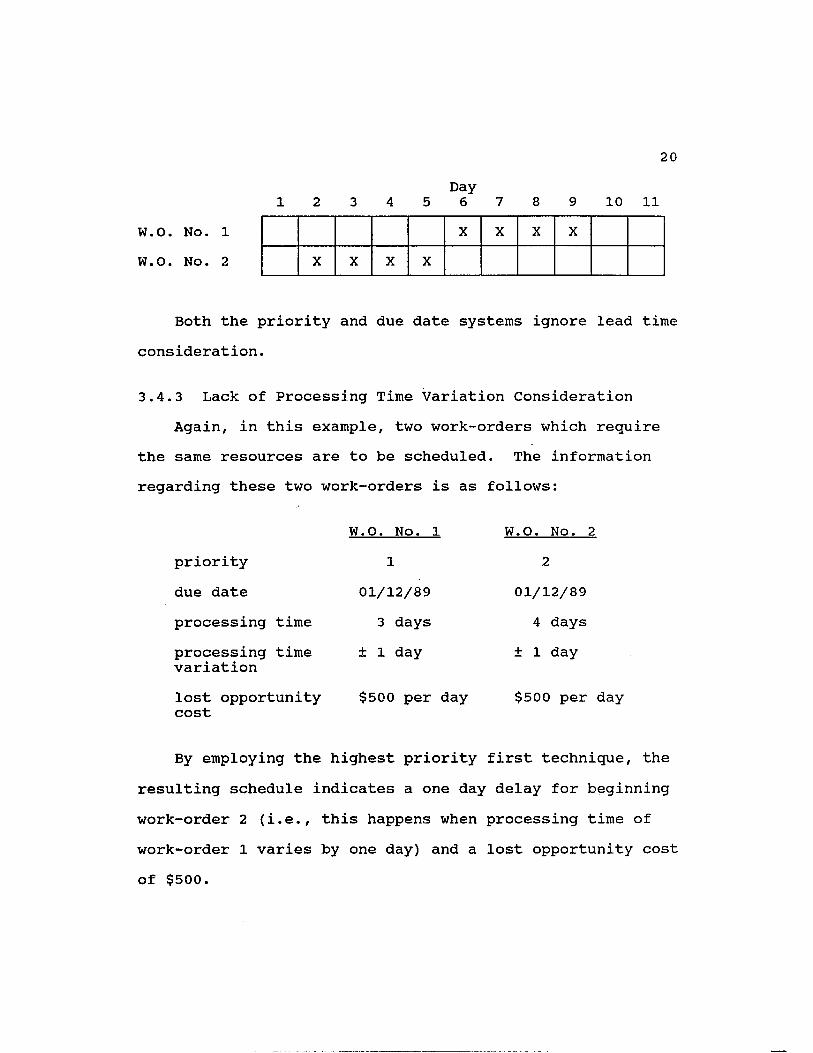
3.4.3 Lack of Processing Time Variation ConsiderationAgain, in this example, two work-orders which require

the same resources are to be scheduled. The information regarding these two work-orders is as follows:

W.O. No. 1 W.O. No. 2priority 1 2due date 01/12/89 01/12/89processing time 3 days 4 daysprocessing time ± 1 day ± 1 dayvariationlost opportunity $500 per day $500 per daycost

By employing the highest priority first technique, the resulting schedule indicates a one day delay for beginning work-order 2 (i.e., this happens when processing time ofwork-order 1 varies by one day) and a lost opportunity costo f $ 5 0 0 .

21

1 2 3 4 5Day6 7 8 9 10 11

W.O. No. 1 X X XW.O. No. 2 X X X X

By first considering the processing time variation, the resulting schedule indicate a zero lost opportunity cost.

Day1 2 3 4 5 6 7 8 9 10 11

W.O. No. 1 X X XW.O. No. 2 X X X X

Both the priority and due date systems ignore work- order processing time variation.

3.4.4 Lack of Lost Opportunity Cost ConsiderationAgain, in this example, two work-orders which require

the same resources are to be scheduled. The information regarding these two work-orders is as follows:

priority due date processing time opportunity cost

W.O. No. 1 2

01/08/89 3 days

$100 per day

W.O. No. 2 2

01/09/89 7 days

$500 per day

By employing the highest priority first technique, the resulting schedule will cause work-order 2 to finish one

22day late and will result in a lost opportunity cost of $500.

Day1 2 3 4 5 6 7 8 9 10 11

W.O. No. 1 X X XW.O. No. 2 X X X X X X X

A1 day late

By considering the large lost opportunity cost to be critically important, work-order 1 will finish two days late, but with an opportunity cost of only $200 (i.e., $100 x 2 days).

Day1 2 3 4 5 6 7 8 9 10 11

W.O. No. 1 X X X X X X XW.O. No. 2 X X X

A 2 days late

Both the priority and due date systems ignore lost opportunity costs.

3.5 Disadvantages of the Current TechniquesThere are several seemingly obvious shortcomings to the

highest priority first and due date scheduling systems.One reason that these drawbacks have not been addressed previously is probably because the approach seems fair. In addition, some maintenance personnel apparently believe

23that there is nothing more they can do when all the maintenance crews are busy. As such, the most obvious solution to any delay or congestion of work-orders is to request more manpower or additional tools for the maintenance work force. (Note: Because of this difficult- to-control situation, many organizations have elected to subcontract their maintenance activities, to pay a fixed (probably high) price to have someone else worry about the problem.)

The success or failure of the priority system depends heavily on many factors. Most factors, such as priority values and due dates, are subjectively set. As such, they are difficult to evaluate. This is especially true since maintenance activities are generally performed as quickly as possible and since they are often unique activities.

As stated above, all production and maintenance personnel involved must understand and respect the priority system in order for it to be effective. This condition is difficult to accomplish, especially in a large plant which has hundreds of personnel involved in its operation.Abuses (overspecification of priority) of the priority system occur when there is pressure on the production department to keep the production process operating. The originators of work-order priorities may often be guilty of increasing the priority index of a job by an extra notch or two in order to expedite their work-orders. In other

24words, if all jobs are given high priority, all jobs have equal priority.

In addition, the priority index system does not show the real effect of maintenance work-orders on the production process in any objective way. That is, there is no quantitative measure of the procedure1s impact on the production process. Two work-orders with the same priority index number may have dramatically different effects on the production process and on organizational profitability. As such, using due dates to break ties between work-orders with the same priority may not be appropriate if all the work-orders are considered to be urgent. The effect of each work-order on the production process in terms of cost (or profit) per unit time should be considered instead.

Following this same line of reasoning, one might suggest that the priority index values be based on profit. If this suggestion is followed, the work-order which affects the higher profit operating unit should be assigned a higher priority than work-orders which affect lower profit operating units. While this concept seems to make sense, it is incomplete. It is not applicable to all possible, meaningful situations. Some operating units, such as a waste treatment unit, do not return any profit but are directly related to several other products' profits. If the waste treatment unit does not perform

25properly, the organization may have to pay a heavy fine and face other unpleasant, unprofitable consequences.

In summary, the due date system is an inappropriate criterion to use for scheduling maintenance jobs. As has been discussed in detail in Chapter 2, there are two distinct types of maintenance jobs, preventive maintenance jobs and emergency maintenance jobs. Often, for the preventive maintenance situation, the due dates assigned to work-orders are largely arbitrary. Typically, the primary concern is exhibited by the production department and its concern is to have the production equipment serviced at the time it is scheduled (e.g., during the night shift when the unit is offline). Any unplanned delays for service may result in an additional loss of production. Using a similar argument, it is equally apparent that emergency maintenance situations frequently have no meaningful due date assignments either. All emergency maintenance situations need (by definition) to be serviced immediately. As such, the only difference between most emergency situations is the effect thte situation has on the production process it affects. Clearly, the effect the inoperative equipment has on the production process and on the plant's profitability is a more appropriate scheduling criterion than an arbitrarily chosen due date.

In later sections, the arguments presented in this chapter to show that the currently used maintenance

scheduling techniques are often inappropriate are revisited from a more positive perspective. The next chapter includes a description of the maintenance scheduling process from the perspective of the costs involved, the basis of a more appropriate scheduling approach.

CHAPTER 4 MATHEMATICAL MODEL OF

THE PROPOSED MAINTENANCE SCHEDULING SYSTEM

Before any quantitative analysis of the maintenance scheduling system can be performed, a model must be constructed. A formal mathematical model of the proposed maintenance scheduling system is presented in this chapter. A description of the model is also presented, following the statement of the mathematical model. Analysis of the proposed maintenance scheduling system is presented in subsequent chapters.

4.1 Mathematical Model Objective Function :Minimize the Total Maintenance Cost= Minimize (Total Preventive Maintenance Opportunity Cost +

Total Emergency Maintenance Opportunity Cost + Total Resource Cost)

= Minimize 2 CPMj • SDTPM• +i=l

2 CEM- • SDTEM• +j=l 3 3

2 CRk • Rk k=l

27

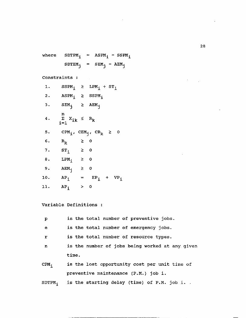
28where SDTPM^

SDTEMj

Constraints :1. SSPMj >2. ASPMi >3. SEMj >

4.nS Xik i=l 11C

<

5. CPMif CEM.6. Rk >7. ST^ >8. LPM^ >9. AEMj >10. Api =11. APf >

= ASPM^ - SSPM^ = SEMj - AEMj

LPM^ + ST^SSPM^AEMj

Rk

, CRk > 00 0 0 0EPi + VP±0

Variable Definitions :

p is the total number of preventive jobs,e is the total number of emergency jobs,r is the total number of resource types,n is the number of jobs being worked at any given

time.CPM^ is the lost opportunity cost per unit time of

preventive maintenance (P.M.) job i.SDTPM• is the starting delay (time) of P.M. job i. ,

29AS PM,SSPM,LPM^

CEMj

SDTEMj

A E M j

S E M j

CRr

XikAP,EP,VP,

is the actual starting time of P.M. job i. is the scheduled starting time of P.M. job i. is the required lead time of P.M. job i. is the time at which P.M. job i is scheduled, is the lost opportunity cost per unit time for emergency j ob j.is the starting delay (time) of emergency job j.is the arrival time of emergency job j.is the starting time of emergency job j.is the unit cost of resource k for the operatingperiod.is the available quantity of resource k. is the amount of resource k required by job i. is the actual processing time for job i. is the expected processing time for job i. is the variation of processing time for job i.

4.2 Description of the Mathematical Model

Objective function :The objective for the maintenance scheduling model is

to minimize the total maintenance-related cost. The totalcost consists of the total preventive maintenance lost opportunity cost, the total emergency maintenance lostopportunity cost, and the total resource cost.

30The total preventive maintenance lost opportunity cost

is the summation of lost opportunity amounts associated with all preventive maintenance jobs. The lost opportunity cost of a preventive maintenance job is the product of the lost opportunity cost per unit time (CPM) and the starting delay time (SDTPM). The so-called starting delay (time) for a preventive maintenance job (SDTPM) is the difference between the actual starting time (ASPM) and the scheduled starting time (SSPM).

Similarly, the total emergency maintenance lost opportunity cost is the summation of lost opportunity costs of all emergency maintenance jobs. The lost opportunity cost of an emergency maintenance job is the product of the lost opportunity cost per unit time (CEM) and the starting delay (time) (SDTEM). The starting delay (time) for an emergency job is the difference between the job's arrival time (AEM) (i.e., when it is learned that the emergency maintenance task must be performed) and the emergency maintenance task's starting time (SEM).

The total resource cost is the total of all resource related costs associated with the maintenance department. Resources include both maintenance crews and maintenance equipment. The cost of each resource type is the product of the unit cost for the operating period (CR) and the available quantity of that resource (R).

31

Constraints :

1. SSPM^ > LPMi + ST^The scheduled starting time of preventive maintenance

job i (SSPM^) cannot take place prior to the job scheduling process. More specifically, the scheduled starting time for preventive maintenance job i must consider the job's lead time and the time at which scheduling is performed. This constraint assures that lead time for preventive maintenance jobs is considered.

2 . ASPM^ > SSPMi

The actual starting time of preventive maintenance job i (ASPM^) cannot occur before the scheduled starting time (SSPM^). This constraint prevents early starts of preventive maintenance jobs. Put another way, the operating unit requiring preventive maintenance need not stop (i.e., be taken offline) before the scheduled preventive maintenance start time.

3 . SEMj > AEMj

No emergency maintenance jobs can start until after the emergency condition has occurred. The logic behind this constraint is obvious.

The summation of all units of resource type k used by all maintenance jobs cannot exceed the available quantity of resource k.

5. CPJ^, CEMj , CRk > 0The lost opportunity cost for each preventive

maintenance task, the lost opportunity cost for each emergency maintenance task, and the unit resource cost must each be nonnegative. This constraint ensures that no negative costs are included in the formulation.

6. Rk > 0The available quantity of resource type k must be

nonnegative.

7. > 0The time at which maintenance scheduling is performed

(for all preventive maintenance tasks i) must be nonnegative.

8. LPM^ > 0The lead time required for preventive maintenance job i

must be greater than or equal to zero.

339. AEMj > 0

The arrival time of emergency job j (i.e., the time at which the emergency condition is recognized) must be greater than or equal to zero.

10. = EP^ + VPdThe actual processing time of maintenance job i differs

from the expected processing time (EP ) by an amount defined by the processing time variation (VP^). Variation of processing time can be either positive or negative. Positive processing variation occurs when the actual processing time is greater than the expected processing time. Negative processing variation occurs when the actual processing time is less than the expected processing time. The actual processing time of maintenance jobs can be greater than, less than, or equal to the expected processing time.

11. AP^ > 0The actual processing time of maintenance jobs must be

greater than zero.

CHAPTER 5 MAINTENANCE SCHEDULING SYSTEM CONSIDERING ONLY EMERGENCY JOBS

This chapter deals with a subset of the total maintenance scheduling system in which only emergency jobs are considered for scheduling. The analysis of this special case is considerably simpler than the analysis of the total maintenance scheduling system introduced in Chapter 4. Nevertheless, the study of such special cases often helps to clarify the general situation and may lead to solutions to the overall problem.

In fact, the maintenance scheduling system which considers only emergency jobs is both a special case and a complete situation in its own right. The situation occurs in reality when a policy of performing no preventive maintenance is adopted by an organization (i.e., maintenance is performed only when there is an equipment breakdown) or when all preventive maintenance activities are subcontracted (i.e., as far as the company is concerned, only emergency maintenance jobs occur).

5.1 Mathematical ModelThe mathematical model for the maintenance scheduling

system considering only emergency jobs can be obtained from the general maintenance scheduling mathematical model presented in Chapter 4 by eliminating the "Total Preventive

34

35Maintenance Opportunity Cost" term. The resulting equation is as follows:

Objective Function : Minimize the Total Maintenance Cost

= Min (Total Emergency Lost Opportunity Cost + Total Resource Cost)

eMin Z

j=l

E.M. Lost Opportunity Cost Related to Scheduling E.M. Job j

+

r2k=l

Resource Cost Related to Resource Type k

Min 2 CEM • • WTEM.J + j=l 3 3

r2 CR k=l k ' Rk

where WTEMj = SEMj - AEMj

Constraints :SEM- > AEM■

Xik ^ Rk1=1

CEMj, CRk4. > 0

3 6

5. AEMj > 0

See Chapter 4 for complete definitions of the above variables and a complete model explanation.

5.2 Brief Discussion of the Mathematical Model and its Constraints

The objective function is composed of two parts, the total emergency lost opportunity cost and the total resource cost. Five constraints further clarify the situation.

Constraints 1, 3, and 5 represent boundary conditions. They ensure that the total emergency lost opportunity cost is nonnegative. The lowest possible value occurs only when all arriving emergency jobs are served immediately (i.e., only when the system has abundant resources to handle all emergency jobs without delay). The total emergency lost opportunity cost increases if there are emergency jobs which cannot begin immediately. It is apparent that total emergency lost opportunity cost is directly related to the availability of resources. While a large resource pool may reduce the total emergency lost opportunity cost, it also increases the total resource cost.

The total resource cost is the summation of the costs for all resources. It is assumed that the resource cost of each resource is a linear function of the quantity of each resource available and their respective resource unit

37costs. It is also assumed that the. resource unit cost is fixed for each resource type, so that only one variable, resource quantity, controls the resource cost of each resource.

5.3 Influence DiagramAn influence diagram1 is an important tool which is

used to illustrate the relationships among attributes and interested variables of a particular system. In some cases, the mathematical model serves inadequately as a tool for communicating or structuring a model. An influence diagram is an ideal tool for describing relationships among all interested variables in a system, whether or not those relationships can be formulated mathematically.

An influential diagram consists of three basic types of variables: decision variables are represented by a rectangle, intermediate variables are represented by a circle, and attribute variables are represented by an ellipse. In addition, the diagram includes the influence relationships among the variables. An influence is a

fdependency of one variable on the level of another variable. In an influence diagram, a certain influence is indicated by a single straight arrow, an uncertain

1 . • •The details of the influence diagram can be found inChapter 3 of "Modern Decision Making" by Samuel E. Bodily (Bodily 1985).

3 8

influence is indicated by an arrow with a squiggle, and a preference dependency is signified by a double straight arrow. Normally, the dependency of a certain influence can be clearly described by a mathematical expression. On the other hand, an uncertain influence indicates the existence of a dependency between two variables that may be difficult, if not impossible, to describe by a mathematical expression. A preference influence reflects an influence on the desirability of the influenced variable, not its level. A preference influence can be used in a situation that calls for decision making to be based on a preferred policy.

Figure 5.1 shows the influence diagram for the maintenance scheduling system considering only emergency jobs. It describes the influences and relationships that system attributes have on the total cost which is the interested variable.

There are three system attributes which serve as parameter variables for each scheduling situation: the arrival process, the rate of lost opportunity cost for each arriving emergency job, and the unit cost for each maintenance resource. The resource level and the scheduling policy are the two decision variables that can

2In this situation, the arrival process includes the rate of arrival and its distribution, the resource requirement, and the processing time.

39

Resource Unit Cost

ArrivalProcess

ResourceCost

TotalCost

Waiting Tine ,

Lost Opp Cost

Rate of Lost Opp

Cost

No. of Waiting Jobs ,

ResourceLevel

SchedulingPolicy

Figure 5.1 Influence Diagram - Emergency Jobs Only

be controlled by the scheduler. The resource level is certainly influenced by the arrival process. The arrival process determines the minimum number of resource levels needed for the maintenance operations. However, the preference for the resource levels is influenced by the

40number of waiting jobs. If the number of waiting jobs is high, the scheduler may decide to increase the resource levels. The number of waiting jobs is a intermediate variable which is certainly influenced by the arrival process, the resource levels and the scheduling policy.The scheduling policy is a decision made by the scheduler for a specific situation based on the scheduling strategy. The waiting time is another intermediate variable that is certainly influenced by the scheduling policy. The waiting time and the rate of opportunity cost directly determine the lost opportunity cost. The resource cost is calculatedfrom the resource level and the resource unit cost.Finally, the summation of both the lost opportunity cost and the resource cost makes up the total cost.

The right set of values for the two decision variablescan result in the desired optimum total cost. It should benoted that the scheduling policy, one of the two decision variables, is the guideline that suggests the order of emergency maintenance jobs to be serviced. The result is a combinatorial problem which cannot be solved by classical methods such as the linear programming technique.

5.4 Maintenance Viewed as a Queueing ModelThe emergency maintenance system can be viewed as a

classical queueing model. Arrivals of emergency jobs are random but can be determined to follow some probability

4 1

distribution by means of experience and maintenance history. Arriving jobs are served immediately, if the required resources are available. If the needed resources are unavailable, the emergency jobs must wait for service. This, of course, is comparable to the situation in which customers wait in a queue.

As with the queueing model, the two major factors affecting emergency maintenance operation are the available quantities of resources (i.e., the number of servers) and the queueing discipline. The "queueing discipline" includes the distribution of arrivals and the order in which these arrivals are chosen for service. The optimum solution to the objective function depends directly on these two major factors.

5.5 Effects of Resource QuantitiesAs discussed previously, arriving emergency jobs go

directly into service (i.e., no waiting), if there are a sufficient resources. This circumstance typically results in a zero lost opportunity cost and a high resource cost situation. The resource cost may be decreased by reducing the resources available, but such a policy increases the chance (and duration) of having arriving emergency jobs wait for service. In short, the tradeoff between the lost opportunity cost and the resource cost is the problem to be studied.

425.5.1 A Look at a Special Case

In this section, a simplified version of the emergency maintenance situation is examined using the assumption of the classical M/M/c queueing model. The only purpose of this assumption of the M/M/c queueing model is to be able to perform sensitivity analysis on the resource level. The intent of this section is to present the relationship, rather than to determine the optimum solution.

This special case is based on several assumptions which are made for the classical M/M/c queueing model. These are listed below.- Arrivals follow a Poisson process with the mean of a jobs per unit time.

- Service times are exponentially distributed at the rate of n jobs per unit time.

- All jobs have the same lost opportunity cost, CEM dollars per unit time.

- Each emergency job requires only one type of resource.The resource cost of each resource is CR dollars per unit time.

- There are c total resources.- The waiting line discipline is first-in first-out (FIFO).

3 .Emergency maintenance jobs may or may not arriveaccording to a Poisson process and may or may not have exponential service times. This "special case" simply examines the situation which uses these two classical assumptions.

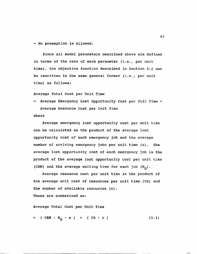
43- No preemption is allowed.

Since all model parameters described above are defined in terms of the rate of each parameter (i.e., per unit time), the objective function described in Section 5.2 can be rewritten in the same general format (i.e., per unit time) as follows:

Average Total Cost per Unit Time= Average Emergency Lost Opportunity Cost per Unit Time +

Average Resource Cost per Unit Time where

Average emergency lost opportunity cost per unit time can be calculated as the product of the average lost opportunity cost of each emergency job and the average number of arriving emergency jobs per unit time (a). The average lost opportunity cost of each emergency job is the product of the average lost opportunity cost per unit time (CEM) and the average waiting time for each job ( W q ) .

Average resource cost per unit time is the product of the average unit cost of resources per unit time,(CR) and the number of available resources (c).These are summarized as:

Average Total Cost per Unit Time

= ( CEM • WQ • a ) + ( CR • c ) (5.1)

44For an emergency maintenance system, all terms in

Equation 5.1 are given except the average waiting time for each job (Wq ). It is interesting to note that the value of the average waiting time ( W q ) is a function of other given system parameters, especially the number of available resources (c).

For the emergency maintenance system (i.e., the M/M/c queueing model), the average waiting time ( W q ) is expressed as follows:

W,

where

(a / n ) •fj,(c-1) ! (c‘fjL - a)

(5.2)

c-1 1 an

1 ac

c *mE

n=0 n! MT

c! c • fj, - a

-1

The average waiting time of emergency jobs ( W q ) for the M/M/c model described in Equation 5.2 is a function of the mean arrival rate (a), the mean service rate of each resource (/tx) , and the number of available resources (c) .In summary, for a given set of mean arrival rate (a) and mean service rate of each resource (/x) values, the average waiting time of emergency jobs ( W q ) is explicitly a function of the number of available resources (c). Table

5.1 shows the resulting W q function for c values of 1, 2,3, and 4.

Number of Available Average Waiting Time ofResources (c) Emergency Jobs ( W q )

a1

M*(M " a) a2

2M* (4 */x2 “ a2)

a33

(18«/Lt3 + 6*/Li2*a - jU*a2 - a3) a4

/Ll* (96 • + 48*/Lt3*a + 6*m2*Q!2 - 2*/j*a3 - a4)

Table 5.1 W q Function for Four c Values

Arrival Rate (a) : 9 jobs per unit timeService Rate (ji) : 10 jobs per unit timeNo. of Resources (c) Average Waiting Time ( W q )

1 0.90002 0.02543 0.00334 0.0005

Table 5.2 Example of Relationship between c and Wq

4 6

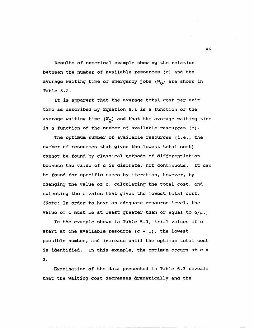
Results of numerical example showing the relation between the number of available resources (c) and the average waiting time of emergency jobs ( W q ) are shown in Table 5.2.

It is apparent that the average total cost per unit time as described by Equation 5.1 is a function of the average waiting time (Wq ) and that the average waiting time is a function of the number of available resources (c).

The optimum number of available resources (i.e., the number of resources that gives the lowest total cost) cannot be found by classical methods of differentiation because the value of c is discrete, not continuous. It can be found for specific cases by iteration, however, by changing the value of c, calculating the total cost, and selecting the c value that gives the lowest total cost. (Note: In order to have an adequate resource level, the value of c must be at least greater than or equal to a//x.)

In the example shown in Table 5.3, trial values of c start at one available resource (c = 1), the lowest possible number, and increase until the optimum total cost is identified. In this example, the optimum occurs at c = 2 .

Examination of the data presented in Table 5.3 reveals that the waiting cost decreases dramatically and the

47resource cost increases linearly as the resource level (c) increases linearly.

Arrival Rate (a) 9 jobs per unit timeService Rate (n) : 10 jobs per unit timeWaiting Cost : 50.00 dollars per unit timeResource Cost : 20.00 dollars per unit per unit timec WQ Waiting Resource Total

Cost Cost Cost1 0.9000 405.00 20.00 425.002 0.0254 11.43 40.00 51.433 0.0033 1.50 60.00 61.504 0.0005 0.21 80.00 80.21

Table 5.3 An Example of Finding Optimum Number of Available Servers

5.6 Selection Rule for Competing Emergency JobsThe emergency-jobs-only maintenance situation can

logically be viewed as a classical queueing system. This does not afford answers to every question, however. Still, a selection rule is needed when there are two or more emergency jobs competing for the same resources. Fortunately, in reality, the probability of this circumstance occurring is often quite low, especially when the optimum number of resources is employed.

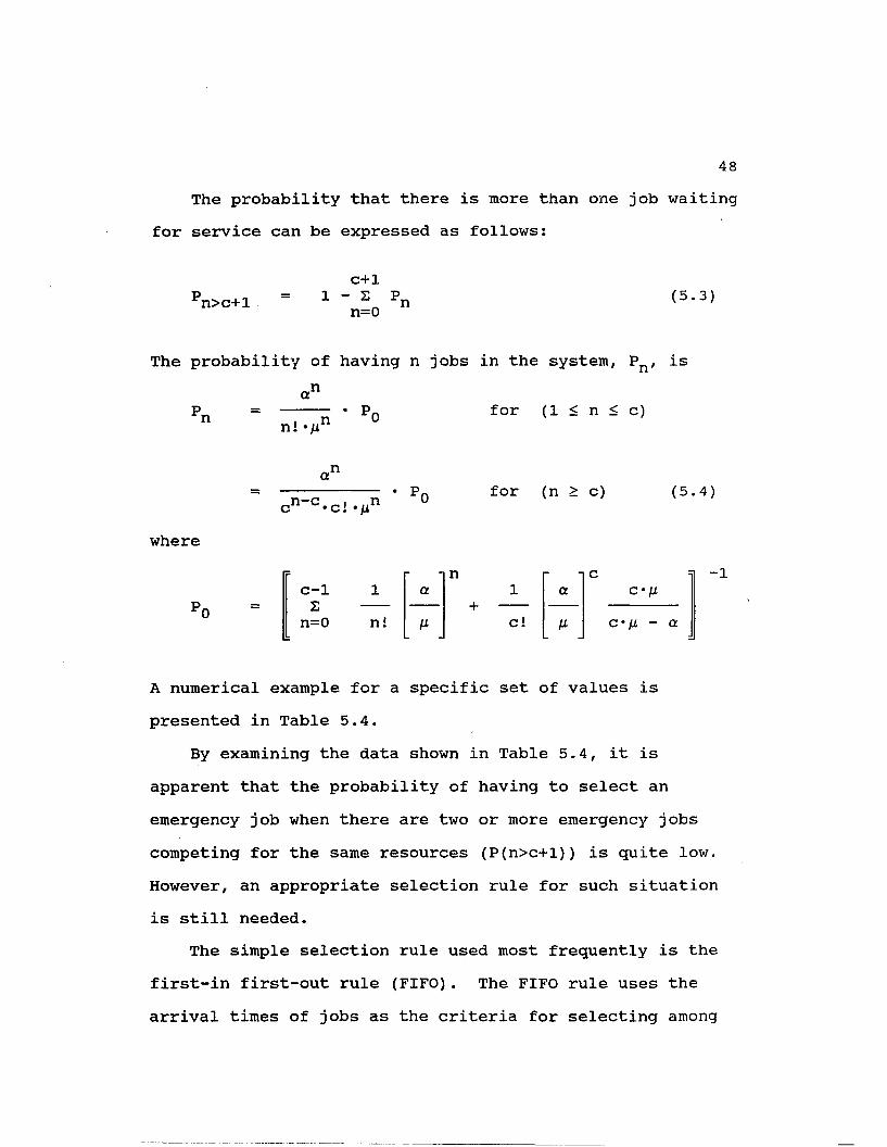
48The probability that there is more than one job waiting

for service can be expressed as follows:

n>c+lc+1

1 - S P n=0 n (5.3)

The probability of having n jobs in the system, Pn, is „.n

n

where

n! n 0

an

cn-c.c!.Mn °

for (1 < n < c)

for (n > c) (5.4)

c-1 i an+

1 ac

C • jLtn=0 n! c! c*/x - a

-1

A numerical example for a specific set of values is presented in Table 5.4.

By examining the data shown in Table 5.4, it is apparent that the probability of having to select an emergency job when there are two or more emergency jobs competing for the same resources (P(n>c+l)) is quite low. However, an appropriate selection rule for such situation is still needed.

The simple selection rule used most frequently is the first-in first-out rule (FIFO). The FIFO rule uses the arrival times of jobs as the criteria for selecting among

49waiting jobs. The first arriving emergency job is served first, then the next arriving job, and so on. The FIFO rule has remained popular because of its simplicity and broad application in general queueing problems. The FIFO selection criteria, however (i.e., the arrival times of emergency jobs), may or may not be appropriate for scheduling emergency maintenance jobs.

Arrival Rate (a jobs per unit time) : 9Service Rate (n jobs per unit time) : 10Probability of having n emergency jobs in system (Pn)

Number of Jobs Number of Available Resources (c) in System (n)

2 3 4

0 0.3793 0.4035 0.40621 0.3414 0.3631 0.36562 0.1536 0.1634 0.16453 0.0691 0.0490 0.04944 0.0311 0.0147 0.01115 0.0140 0.0044 0.00256 0.0063 0.0013 0.00067 0.0028 0.0004 0.00018 0.0013 0.0001 0.00009 0.0006 0.0000 0.000010 0.0003 0.0000 0.0000

P(n>c+1) 0.0566 0.0063 0.0007

Table 5.4 Probability of Having n Jobs in System

50

5.7 Consequences of Selecting an Emergency JobAs described previously, a selection must be made when

there are two or more emergency maintenance jobs competing for the same resources. No matter which job is selected, there are still one or more other jobs waiting as the result of the selection process. This waiting results in a lost opportunity cost. Better selection rules should result in lower lost opportunity costs. A model which considers the lost opportunity cost is developed in this section. The model is intended to help us understand the situation and allow us to determine another selection rule for choosing between competing emergency jobs.

When selecting a job to be worked, an immediate lost opportunity cost occurs as a result of the remaining n waiting jobs. This can be expressed as follows:

Immediate Consequential Lost Opportunity Cost = S •C^ + S •C2 + ... + S •Cn

rS • Z Ci (5.5)

i=lwhere

S is the processing time of the selected job,C^ is the lost opportunity cost per unit time of the

ith j ob, and r is the number of remaining waiting jobs.

51Equation 5.5 indicates that the immediate lost

opportunity cost is a function of the processing time of the selected job (S) and the total lost opportunity cost per unit time of the remaining jobs.

There is no reason to include an arrival time component in this model. Because the first-in first-out (FIFO) selection rule uses arrival time as the primary selection criteria and because that selection rule ignores all possible cost ramifications of the selection process, it can be reasonably concluded that the first-in first-out selection rule is not an appropriate selection rule for this situation.

The emergency maintenance scheduling problem may be viewed as a sort of combinatorial minimization problem (e.g., similar to the famous traveling salesman problem). The emergency maintenance scheduler tries to find the optimum schedule, which is comprised of a combination of emergency jobs that yields the lowest total lost opportunity cost. The difference between the classical combinatorial minimization problem and the emergency maintenance scheduling problem is the state of the problem. The classical combinatorial problem can be viewed as a static problem in which all needed information is known at the beginning and does not change from start to finish. On the other hand, the emergency maintenance scheduling problem must realistically be viewed as a dynamic problem

52in which new emergency jobs may arrive after the schedule has been set. This important difference prevents us from applying the classical algorithm to the emergency maintenance scheduling problem. However, using the immediate lost opporutunity cost as the primary decision criteria, the following sections present selection rules which attempt to make choices that result in the minimization of Equation 5.5.

5.8 The Method of Total EnumerationFor the static emergency maintenance scheduling problem

(i.e., one in which no new jobs arrive after the schedule is set until the last job is completed), the set of all possible scheduling sequences is finite. The optimum solution, which is certain to be a member of this set, can be found by the method of total enumeration. The method of total enumeration involves calculating the total lost opportunity cost for each member of the set. For a specific sequencing order, the total lost opportunity cost is the summation of all individual lost opportunity costs until all jobs are completed. The optimum solution is the sequencing order that yields the lowest total lost opportunity cost.

5.8.1 Example of the Method of Total EnumerationThis example demonstrates the scheduling process which

uses the method of total enumeration. Three emergency

53maintenance jobs are to be scheduled sequentially. The data are shown below:

Expected Processing Lost Opportunity Job Time (hours) Cost (dollars per hour)

A 3 35.00B 4 42.00C 5 29.00

All possible scheduling sequences and their respective total lost opportunity costs are as follows:

Sequencing Total LostOrder Opportunity Cost (dollars)

A - B - C 3* (42 + 29) + 4* (29) = 329A - C - B 3* (42 + 29) + 5 •(42) = 423B - A - C 4* (35 + 29) + 3* (29) = 343B - C - A 4* (35 + 29) + 5* (35) = 431C - A - B 5* (35 + 42) + 3* (42) = 511C - B - A 5* (35 + 42) + 4* (35) = 525

For this example, selecting Job A first, then Job B second and finally Job C is the optimum alternative, the one which produces the lowest total lost opportunity cost.

5.9 The Method of One-Step TrialThe problem with the method of total enumeration is

that as the number of jobs increases linearly, the number

54of possible scheduling sequences increases exponentially.In order words, if the number of alternative jobs is large, computation time may become a problem. One logical selection method, a simplification of the method of total enumeration, may be referred to as the method of one-step trial. Step one is to choose any job as the first job for scheduling and calculate the immediate (i.e., for the time period of the selected job) lost opportunity cost by Equation 5.5. Repeat the process for all waiting jobs. Select as the first scheduled job the one producing the lowest immediate lost opportunity cost. Once the first job to be scheduled is chosen, eliminate it from the group of possible candidates and repeat the procedure to determine the second job to be scheduled. Repeat the procedure until all jobs have been scheduled.

The method of one-step trial schedules emergency maintenance jobs based on the lowest immediate lost opportunity cost. Instead of going through the entire sequencing order and calculating the total lost opportunity cost as in the method of total enumeration, the method of one-step trial considers only one step in the selection sequence. By considering only one step at a time, the number of calculations can be reduced significantly. For example, there are 120 different sequencing alternatives for five emergency maintenance jobs (5!). The method of total enumeration needs 120 calculation steps to determine

55the optimum sequence while the method of one-step trial needs only 14 calculation steps (5+4+3+2).

This method is logical and may be particularly effective, in solving the dynamic emergency maintenance scheduling problem in which new emergency jobs may arrive or some scheduled emergency jobs may be cancelled after the schedule has been set. It does not guarantee the selection of the sequence with the lowest total lost opportunity cost, which is the stated objective of the emergency maintenance scheduling problem, but it does guarantee the selection of the job having the lowest immediate lost opportunity cost.

In an attempt to determine the effectiveness of the one-step trial method, a simulation for three waiting jobs was performed. It was found that the method of one-step trial results in the same optimum solution as the method of total enumeration in 91 percent of the cases (based on a long term simulation of three waiting jobs situation).

5.9.1 Example of the One-Step Trial MethodThis example demonstrates the scheduling process which

uses the method of one-step trial. A single job is selected from a pool of three waiting emergency jobs. The data are shown below:

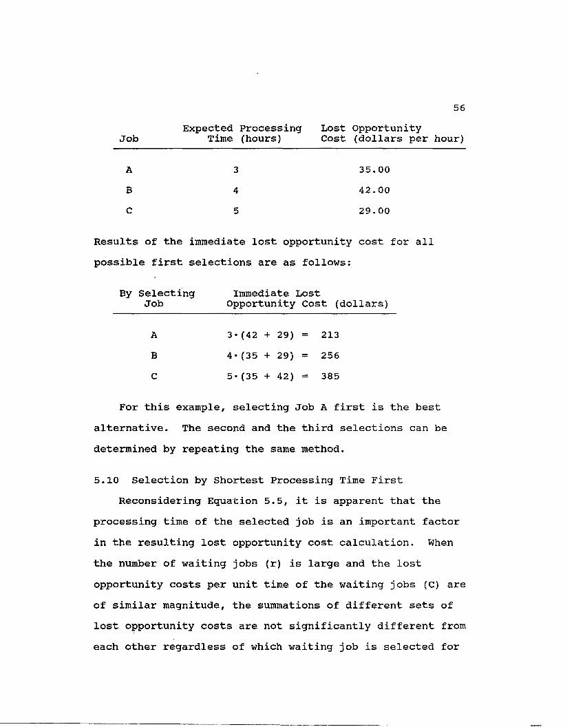
56Expected Processing Lost Opportunity

Job Time (hours) Cost (dollars per hour)

A 3 35.00B 4 42.00C 5 29.00

Results of the immediate lost opportunity cost for all possible first selections are as follows:

By Selecting Immediate LostJob Opportunity Cost (dollars)

A 3* (42 + 29) = 213B 4*(35 + 29) = 256C 5*(35 + 42) = 385

For this example, selecting Job A first is the best alternative. The second and the third selections can be determined by repeating the same method.

5.10 Selection by Shortest Processing Time FirstReconsidering Equation 5.5, it is apparent that the

processing time of the selected job is an important factor in the resulting lost opportunity cost calculation. When the number of waiting jobs (r) is large and the lost opportunity costs per unit time of the waiting jobs (C) are of similar magnitude, the summations of different sets of lost opportunity costs are not significantly different from each other regardless of which waiting job is selected for

57scheduling. If this is the case, to select jobs based on the shortest processing time (S) is an effective strategy. Although this scheduling approach does not guarantee the lowest total lost opportunity cost, it does provide a high probability of choosing the emergency work-order whose resulting lost opportunity cost is lowest.

The major advantage of this method over the method oftotal enumeration and the one-step trial method is its simplicity. No calculations are needed. The simplicity of this method is comparable to the first-in first-out (FIFO) scheduling method, but has the important advantage of having a sound theoretical basis.

For the example in Section 5.9.1, Job A (which has the smallest expected processing time) is scheduled first byusing the shortest processing time decision criteria. Inthis case, the selection of Job A yields the minimum lost opportunity cost.

5.11 Selection by Largest Lost Opportunity Cost FirstLargest lost opportunity cost first is another

selection alternative which appears to be reasonable for the situation that has a large number of waiting jobs (i.e., when r is larger than three). The shortest processing time first approach discussed in Section 5.10 may not be effective when there are one or more waiting jobs with significantly higher lost opportunity cost than

5 8

the lost opportunity costs of the other waiting jobs. In such cases, it is more appropriate to select the job with the largest lost opportunity cost first. By selecting the job with the largest lost opportunity cost, the largest cost is avoided (i.e., excluded from the summation term of Equation 5.5), resulting in a lower total cost.

As was true with the shortest processing time first method, this method does not guarantee the lowest lost opportunity cost either. However, there is a strong possibility that this approach will yield the lowest cost when applied in similar situations.

In summary, this scheduling method is applicable in situations in which individual emergency jobs have significantly different lost opportunity costs, given that there are no significant differences in their processing times.

5.11.1 Example of the Largest Lost Opportunity Cost First Selection Rule

This example demonstrates the largest lost opportunity cost first selection method. Suppose that there are four waiting jobs with the following characteristics.

59Expected Processing Lost Opportunity

Job Time (hours) Cost (dollars per hour)

A 3 30.00B 4 40.00C 5 20.00D 4 200.00

Job D, with the largest lost opportunity cost (i.e., 200.0), would seem to be the best selection. Subsequent calculations show that selecting Job D is indeed the best decision, at least in the short term.

By Selecting Immediate LostJob Opportunity Cost (dollars)

A 3* (40 + 20 + 200) = 780B 4* (30 + 20 + 200) = 1000C 5* (30 + 40 + 200) = 1350D 4* (30 + 40 + 20) = 360

5.12 Hybrid Scheduling Strategy for Emergency JobsAt this point, it is appropriate to propose a hybrid

scheduling strategy plan for the emergency-jobs-only situation based on the findings of this chapter.

Step 1 Determine the optimum resource level using the simplifying assumptions of the queueing-view technique described in Section 5.5.

6 0

Step 2 If the needed resources are available, all arriving emergency jobs should be processed immediately.

Step 3 If the emergency job's required resources are not available when the need for the emergency job becomes apparent, apply the following selection rules for specific situations:a) If only one emergency job is waiting for service, start the job as soon as the resources are available.b) If two or more jobs are waiting for service, ...

(1) Apply the shortest processing time first rule and calculate the immediate lost opportunity cost.

(2) Apply the largest lost opportunity cost first rule and calculate the immediate lost opportunity cost.

Select the schedule that yields the lowest immediate lost opportunity cost.

It is apparent that the proposed scheduling plan is more complicated than the currently popular maintenance scheduling technique. There are more calculations required and lost opportunity costs must be estimated in order to use the proposed plan. On the other hand, the proposed hybrid plan may be significantly simpler to cumpute than the one-step plan and dramatically simpler than the total enumeration method. Before comparing the hybrid plan with these two methods, however, it is compared (in the next

61section) with three other approaches we have already discussed.

5.13 Testing a Variety of Scheduling Strategy PlansIt is interesting to compare the hybrid scheduling

strategy plan introduced in Section 5.12 to other classical scheduling techniques and to the currently-popular maintenance scheduling technique (discussed in Chapter 3). The test was performed using discrete simulation. A simulation model was formulated for each scheduling technique. All models were tested under the same operating environment (i.e., same arrival and serving processes) and with common random numbers in such a way that all models were subjected to identical circumstances. This synchronization was used to help assure a valid statistical comparison. After a number of repetitive runs, the results of each model were compared statistically to each other.The scheduling techniques tested are as follows:

a) Proposed Hybrid Emergency Scheduling Strategy,b) Shortest Processing Time First (SPT),c) Highest Opportunity Cost First (HOCF), andd) First-in First-out (FIFO).

(Note: The currently popular maintenance scheduling technique, which is based on the priority index system method, can be viewed as being the same as the Highest Opportunity Cost First method because the priority index

62system, which is based on the relative importance of work- orders, can be calibrated in terms of dollars.)

The four simulation models were coded in SIMAN. The listings and descriptions of the four models are presented in Appendix A.

Arrival Process : Poisson with the rate of 1 job perunit time.

Serving Process : Exponential with 1 resource and therate of 0.8 job per unit time.

Lost Opportunity Rate : Uniform between 0 and 100dollars per unit time.

Average Lost Opportunity CostReolication PROPOSED SPT HOCF FIFO

1 89.88 104.53 95.22 244.452 49.24 56.03 62.21 97.203 61.24 69.31 75.89 127.844 66.95 76.44 84.35 168.745 74.14 85.70 92.73 168.906 102.32 117.31 126.85 275.597 56.55 64.40 64.21 129.558 50.15 57.05 63.39 91.999 74.49 86.75 92.79 212.6710 55.92 65.92 71.63 129.32

Table 5.5 Results of 10 Simulation Runs

63Ten replications for each model were run with 1,100

time units per replication. Since the maintenance scheduling process is a steady-state process, the results from the first 100 time units of each replication were disregarded to assure that the transient period was excluded from testing. As a result, 1,000 time units consisting of approximately 1,000 observations for each replication were included in the tests. Table 5.5 shows the results in terms of the average lost opportunity cost for ten runs of each of the four models.

Reolicate SPT-Prooosed HOCF-Prooosed FIFO-Prooosed1 14.65 5.34 154.572 6.79 12.97 47.963 8. 07 14.65 66. 604 9.49 17.40 101.795 11. 56 18.59 94.766 14.99 24.53 173.277 7.85 7.66 73.008 6.90 13.24 41. 84.9 12.26 18.30 138.1810 10. 00 15.71 73.40

Table 5.6 Pairwise Differences in Lost Opportunity Costs Between the Results of the Proposed Plan and the Results from the Other Methods

300 AVG. OPPORTUNITY COST

PR O P O SE D PLAN

4 5 6 7

R E P L I C A T I O N NO,

S 3 S P T RULE H W G F R U L E E § § § F I F O

Figure 5.2 Comparison of the Four Scheduling Plans

65Figure 5.2 shows a comparison of these four scheduling

plans. Table 5.6 shows the pairwise differences between the proposed plan and the other three scheduling techniques. The results from the proposed plan are better than the results from the other methods in all cases.

Appropriate statistics for the comparison of two simulated systems with correlated sampling are presented by Banks and Carson in their text (Banks 1984) as follows:

1 RSample Mean Difference, D = • 2 D (5.6)

R r=lwhere

Dr = Yrl " Yr2'Yr is the average lost opportunity cost observed

during replication r for model i, and R is the number of replications.

The Sample Variance of the differences is computed by

1 R 2 Var = * 2 (D - D) (5.7)R - 1 r=l

The Standard Error of the differences is estimated by

S = SQRT (Var / R) (5.8)

A two-sided 100(1 - a)% confidence interval for the mean difference, D, is of the form

66D ± V2,v ‘ S <5'9>

whereta/2 v is the 100(1 - a/2) percentage point of a t

distribution with v degrees of freedom, and v is the number of degrees of freedom = R - 1.

By applying Equations 5.6 - 5.9 to the data in Table 5.6, confidence intervals of the mean differences of the comparisons between the proposed plan and the other three scheduling techniques were obtained. These are shown in Table 5.7.

SPT-Proposed HOCF-Proposed FIFO-ProposedMEAN (D) 10.26 14 .84 96.54VARIANCE (Var) 9.10 30.57 2039.74STANDARD ERROR (S) 0.95 1.75 14.2895% C.I. (8.10,12.41) (10.89,18.79) (64.26,128.81)99% C.I. (7.16,13.36) (9.16,20.52) (50.12,142.95)

Table 5.7 Statistics of Differences between theResults of the Proposed Plan and Other Plans

From an inspection of Table 5.7, it is apparent that the confidence intervals of differences between the results of the proposed plan and the results of the other scheduling methods do not include zero at either the 0.05

67or 0.01 levels of significance (i.e., for either 95 or 99 percent confidence intervals). So, it may be concluded statistically that the proposed plan provides a lower average lost opportunity cost than any of the other emergency maintenance scheduling techniques.

From inspection of Table 5.7, it is clear that the proposed plan is "better” than the other classical methods.

5.14 Comparison of the Proposed Hybrid Approach with the One-Step Trial Method

The next question is, "Is the proposed plan as good as the method of one step trial?" This is an important consideration since it is already known that the one-step trial method is nearly as effective as the total enumeration approach. A simulation was performed to test the hypothesis that there is no significant difference between the results produced by these two methods.

Two simulation models were tested under the same conditions used for the test runs performed previously.The listings for the simulation models can be found in Appendix A.

Table 5.8 and Figure 5.3 show the results in terms of the average lost opportunity cost for these simulation tests. It is apparent that the results are quite similar.

A paired-sample t test was set up to test the null hypothesis shown below.

68Hq : There is no significant difference between the

average lost opportunity cost produced by plans developed by the proposed hybrid scheduling method and those developed by the one-step trial method.

H_ : There is a difference.a

Average Lost Opportunity CostReplication Proposed Plan Trial Method Differences

1 89.88 84.78 5.102 49.24 48.39 0.853 61.24 60.90 0. 344 66.95 65.43 1.525 74 .14 72.02 2.126 102.32 101.23 1. 097 56.55 55.98 0. 578 50.15 50.15 0. 009 74.49 73.02 1.4710 55.92 55.50 0.42

MEAN DIFFERENCES (D) 1. 35SAMPLE VARIANCE (Var) 2 .1595% CONFIDENCE INTERVAL (0.30, 2.40)99% CONFIDENCE INTERVAL (-0.16 ,2.85)

Table 5.8 Statistics of Differences between theProposed Plan and the Method of One-Step Trial

69

110

100

90

80

70

60

50

30

20

10

10

REPLI CAT ION NO.r\Xl TRIAL METHOD\7~z\ PROPOSED PLAN

Figure 5.3 Comparison between the Proposed Plan and the Method of One-Step Trial.

Xn - /in 1-35 “ 0 1.35t = --------— = = = 1.98SD / n 2.15 / 10 0.68

^-1,0 “ t10-l,0.05 " 1*833 < 1 ‘9 8 > reject HQ

t„ , ^ = tQ n n, = 2.821 > 1.98, cannot reject H_n-l,a 9,0.01 ' J o

The statistical results indicate that the null hypothesis must be rejected at the 0.05 level of

70significance, but that it cannot be rejected at the 0.01 significance level. In other words, the two methods produce results which are not clearly different from each other, although the one-step trial method consistently results in a lower lost opportunity cost. (Note : The 95% and 99% confidence intervals shown in Table 5.8 provide similar meanings.)

CHAPTER 6 MAINTENANCE SCHEDULING SYSTEM CONSIDERING ONLY PREVENTIVE JOBS

The maintenance situation in which only preventive jobs exist is analyzed in this chapter. Unlike the situation described in Chapter 5 which considers only emergency jobs, the maintenance situation discussed in this chapter considers the case of no emergency maintenance jobs. This special case rarely exists in reality in its purest sense because all equipment breaks down periodically, no matter how good its quality and how much preventive maintenance is performed. However, a system with only a small number of emergency jobs can logically be assumed to serve as a preventive-maintenance-jobs-only system. This assumption allows a study to be focused only on the preventive maintenance work order scheduling system, rather than on a more complete, but more complex, maintenance system.

6.1 Mathematical ModelThe mathematical model for the maintenance system with

only preventive jobs can be obtained by eliminating the "Total Emergency Opportunity Cost" term from the general mathematical model presented in Chapter 4, leaving only the "Total Preventive Maintenance Opportunity Cost" and "Total Resource Cost" terms.

71

Objective Function : Minimize the Total Maintenance Cost

Min (Total Preventive Lost Opportunity Cost + Total Resource Cost)

PMin £ i=l

P.M. Lost Opp. Resource Cost relatedCost for + to performing P.M.Situation i on Situation i

Min £ CPMj • SDTPM • +i=l

r£ CR k=l k * Rk

where

Constraints

WTPM.^ ASPMi - SSPM^

1. SSPM^ > LPM^ +2. ASPM^

n

> SSPM^

3. 2 xik i=l 1K< Rk

4. CPMif CRk > 05. Al*« 06. ST > 07. LPM^ > 08. APi = EPjl +9. APi > 0

73Chapter 4 contains definitions of all the above

variables and a complete model discussion.

6.2 Brief Discussion of the Model's Objective FunctionFor the preventive-maintenance-jobs-only case, the

objective function consists of two cost categories, the preventive maintenance lost opportunity cost and the resource cost. A preventive maintenance lost opportunity cost is incurred when a preventive maintenance job is unable to start at the scheduled time. The total lost opportunity cost of each job is the product of the delayed starting time increment and the lost opportunity cost per unit time for that job. The resource cost is composed of the product of the maintenance resources required to perform each job and the unit cost of each resource. The optimum preventive maintenance scheduling sequence should minimize the sum of the total lost opportunity costs and the total resource costs.

6.3 Influence Diagram1Figure 5.1 shows an influence diagram for the

maintenance scheduling system considering only preventive jobs. It describes the influences and relationships that system attributes have on the total cost, the variable of interest.

1See Section 5.3 for more details and description of the influence diagram.

74

ResourceLevelRate of Arrival

ResourceIdlei Tine JProc. Tine .Variation^ SchedulingPolicy Resource V Cost>

Resource Unit CostLead Tine RequirementStarting i Delay , \ Tine / TotalCostEarly Start Possibility.

Rate of Lost Opp. Cost

Lost Opp Cost

Figure 6.1 Influence Diagram for Preventive Maintenance Scheduling System

Four attributes associated with each preventive maintenance job that certainly influence the scheduling policy: the processing time variation, the lead time requirement, the early start possibility, and the rate of lost opportunity cost. The scheduling policy, one of the two decision variables, is also influenced by the resource unit cost in a trade-off situation between the resource cost and the lost opportunity cost (discussed later in this chapter). The resource level, another decision variable,

75is certainly influenced by the rate of arrival of preventive maintenance jobs. A minimum resource level is required by the rate of arrival. There are two possible outcomes from all decisions made by the scheduling policy: the resource idle time and the starting delay time. These two intermediate variables contribute directly to the resource cost and the lost opportunity cost by which make up to the total cost.

6.4 System with No Processing Time*VariationIf all preventive maintenance jobs require the exact

time specified by their time standard, the jobs can then be said to have no processing time variation (VP^ = 0, for all i). In such a case, the actual processing time of a job is equal to its expected processing time (i.e., AP^ = EP^, as stated by constraint Number 8). This means that all preventive maintenance jobs finish at their expected finish time. This results in no delayed starts for subsequent jobs (i.e., jobs scheduled to begin after the completion of this job). It can be argued that no lost opportunity cost is incurred when all jobs are completed at the time they are scheduled to finish. The scheduling for such cases can be performed successfully using the classical Gantt Chart technique.

If the lost opportunity cost portion of the equation is zero, the only remaining cost in the objective function for

76this case is the resource cost. To minimize the resource cost, it is simply necessary to minimize the number of resources used to perform the preventive maintenance jobs. The minimum number of resources for preventive maintenance can be computed as the minimum number of resources of type j ( R j ) that satisfies the relation shown below:

aj

or

whereaj

J

> =At

INTaj/t

(6.1)

is the arrival rate of preventive maintenance jobs that require resource j,is the service rate of preventive maintenance jobs requiring resource j, andis the required number of resources of type j.

To avoid system overflow,

Rj

That is, the arrival rate of preventive maintenance jobs must not be greater than the service rate times the number of resources for all jobs.

776.4.1 Example of System with No Processing Time Variation

An automobile lubrication station of a car fleet company can be treated as a preventive maintenance system with no processing time variation. If, for example, the mean service time of this lubrication station for all cars in the company fleet is 15 minutes (i.e., the service rate (M) is 4 cars per hour) and the mean arrival rate (a) of cars that require lubrication service is 3 cars per hour, then the number of lubrication stations that the company needs can be computed by Equation 6.1 as follows:

34 1

The result indicates that the required number of lubrication stations is one. Since the processing time of each arriving car is known, the service time of each particular car can be scheduled successfully using the classical Gantt Chart technique. Since this situation represents a perfect scheduling state, arriving cars will not have to wait for service. As a result, no lost opportunity cost will be incurred. The maintenance system can then operate at minimum total cost.

786.5 System with Processing Time Variation

Processing time variation (i.e., the difference between how long a preventive maintenance job actually requires and how long we thought it would require) is a key issue in preventive maintenance scheduling. Significant processing time variation can disrupt the scheduled starting times of subsequently scheduled preventive maintenance jobs, if the scheduler does not somehow account for the processing time variation. The amount of processing time variation is a function of the type of preventive maintenance job.

Obviously, there are two types of variation, negative variation and positive variation. Negative variation occurs when a maintenance job requires less time than expected to finish. Positive variation occurs when a maintenance job requires more time than expected to complete. Only positive variation delays subsequent preventive maintenance jobs. Negative variation affects maintenance scheduling by underutilizing resources, but does not result in delayed starts for subsequent jobs.

Positive processing time variation may cause subsequently scheduled jobs to start behind schedule. A starting delay generates a lost opportunity cost by having precommitted production equipment sit idle instead of being productively used. Minimizing lost opportunity cost will reduce the total preventive maintenance cost and more efficiently use available resources.

79Positive processing time variation becomes a factor in

maintenance scheduling only if there are two or more preventive maintenance jobs which require the same resources and which are scheduled to start immediately or nearly immediately after each other. As such, only this situation is analyzed.

Negative processing time variation results in maintenance resources having idle time. This idle time becomes important if the resource cost per unit time is high compared to the lost opportunity cost which results for waiting jobs. Negative processing time variation will be discussed in a subsequent section.

6.6 Reduction of Lost Opportunity Cost by Increasing Available ResourcesAs stated previously, positive processing time

variation can cause a delayed start only if there are two or more preventive maintenance jobs requiring the same resources and these jobs are scheduled after each other. Therefore, when the probability of having two or more preventive maintenance jobs which require the same resources is minimized, the lost opportunity cost is also minimized. The probability of such a situation occurring is a function of the available number of required resources.

8 0

For preventive maintenance jobs which require one unit of resources and do not have a lead time requirement, a classical queueing model can be used directly for analysis. For the maintenance system which assumes a Poisson arrival process and exponentially distributed service times (i.e., M/M/c queueing model), the probability of having N jobs in the maintenance system can be expressed as follows:

nan

n!-nn 0for (1 < n < c)

n cn_c*c! */ifor (n > c)

(6 .2)

where

c-1 1 an

1 ac 1

0 • t:

•2j ...

n=0 n!+

c! M c*/x - a

-1

a is the average rate of resource requirement associated with arriving jobs,is the average rate of resource usage associatedwith arriving jobs, andis the number of available resources.

The probability of two or more jobs needing the same resources concurrently is the probability of having concurrently addressable jobs whose required resources are

81greater than the number of resources available. This situation may be expressed as:

c1 - S (6.3)

i=0

is the probability of having i jobs in the system, is the number of available resources, and is the probability of having jobs requiring more resources than are available.

It is quite obvious that the situation of having two or more jobs need the same resources will always occur when the number of required resources is greater than the number of available resources. As such, Equation 6.3 represents the probability of having a lost opportunity cost situation. Because the situation is probabilistic, the lost opportunity cost may not occur at all, even when the number of jobs which need the same resources is higher than the number of available resources. However, the lost opportunity cost will never occur as long as the resources needed for the known jobs are less than or equal to the number of available resources. By increasing the number of available resources, the probability of never incurring a lost opportunity cost can be increased. Unfortunately, each additional resource adds to the total resource cost.

Pn>c

wherePlcPn>c

82As such, trade-off analysis must be performed to justify each additional resource.

The reduction of the probability of lost opportunity cost by increasing the number of available resources makes sense when the cost of additional resources is low compared to the lost opportunity cost that results from any delayed start. This approach is also appropriate when processing time variation is high.

Some preventive maintenance jobs may be performed immediately upon recognition, while others have a lead time requirement. Naturally, the time that a job spends in the system is in general longer for those jobs which have longer lead time requirements. Also, if the needed resources are assigned and committed to scheduled jobs at the scheduling time, the number of available resources which are required for lead time jobs to reach the same able-to-be-worked probability level is higher than when no lead time is considered.

6.7 Scheduling One Job at a TimeThe effect of processing time variation can be

eliminated entirely by scheduling one job at a time. Using this approach, each preventive maintenance job is scheduled only when its needed resources are available. This can be achieved by scheduling the next job after the job currently in service is completed. Using this approach, the

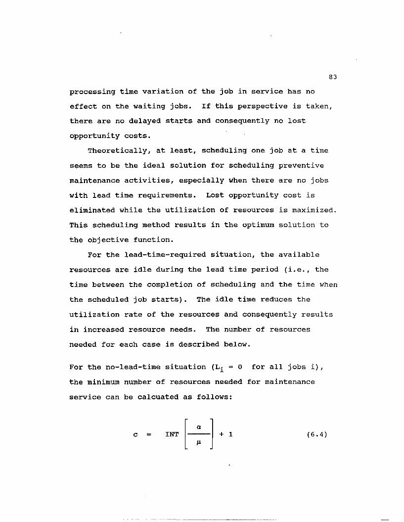
83processing time variation of the job in service has no effect on the waiting jobs. If this perspective is taken, there are no delayed starts and consequently no lost opportunity costs.

Theoretically, at least, scheduling one job at a time seems to be the ideal solution for scheduling preventive maintenance activities, especially when there are no jobs with lead time requirements. Lost opportunity cost is eliminated while the utilization of resources is maximized. This scheduling method results in the optimum solution to the objective function.

For the lead-time-required situation, the available resources are idle during the lead time period (i.e., the time between the completion of scheduling and the time when the scheduled job starts). The idle time reduces the utilization rate of the resources and consequently results in increased resource needs. The number of resources needed for each case is described below.

For the no-lead-time situation (L = 0 for all jobs i), the minimum number of resources needed for maintenance service can be calcuated as follows:

aINT ----- + 1 (6.4)

84where

ca

M

is the minimum number of the resources required, is the average rate of resource requirement associated with the arriving jobs, and is the average rate of resource usage associated with the arriving jobs.

With the lead time constraint (L f 0), the minimum number of resources needed can be calculated as follows:

whereTc

c = INT TS + TL + 1

is the average service time (Tg = ) ,

(6.5)

is the average lead time requirement, and

Ta is the average time between arrivals (TA =a

Equation 6.4 can be rewritten as

c = INT + 1 (6 .6)

Comparing Equation 6.5 with Equation 6.6, it is apparent that the number of required resources must be higher for jobs with lead time.

85If the lead time requirement is small, such that the

number of resources needed (i.e., from Equation 6.5) is essentially the same as the result calculated from Equation 6.6 for the no-lead-time situation, the one-job-at-a-time scheduling method will still be the best scheduling technique for preventive maintenance and will create no lost opportunity cost.

This scheduling method may also be appropriate for the situation in which the resource cost is low compared to the lost opportunity cost that may be incurred because of a delayed start. The additional resources are justified when the resource cost is low compared to the lost opportunity cost.

The one-job-at-a-time scheduling approach is often considerably more effective than the method of increasing the number of resources discussed in the previous section. However, it is not applicable in all situations. When the required lead times of the preventive maintenance jobs are large, the one-at-a-time scheduling method may not yield the optimum solution. The large lead time tends to create an excess of resource idle time. That is, more resources are placed in a waiting state while the utilization of each resource is low.

To increase the resource utilization, these waiting state resources may be assigned to other jobs that have processing times whose duration are less than the idle time

8 6

period. This approach then becomes more-than-one-job-at-a- time scheduling. Such an approach does not guarantee a zero lost opportunity cost because the jobs that are scheduled during the lead time period may require longer time than expected to complete. That is, when the processing time for the in-between-job exceeds the lead time period, the result is a delayed start of the regularly scheduled job. Consequently, a lost opportunity cost is incurred. Still, this approach is appropriate when the immediate, in-between jobs have no positive processing time variation or when the estimated lost opportunity cost for the subsequent, regularly scheduled job is lower than the resource cost which would be wasted if no in-between jobs are scheduled.

6.8 Planned Time Gap TechniqueThis technique uses the sensible approach of inserting

a scheduled time gap between two preventive maintenance jobs that require the same resources and in which one job is scheduled to follow the other and the second job must

lstart at the planned time. The time gap serves as a buffer, reducing or eliminating the effect of the positive processing time variation. The time gap buffer allows the positive processing time variation of the first job to vary by an amount equal to the time gap without having any impact whatsoever on subsequently scheduled jobs. Of

87course, the size of the time gap directly affects the probability of a delayed start for the subsequent job. The larger the time gap, the smaller the chance of a delayed subsequent job start. Also, even if a delayed start does occur, the delay time will be reduced. On the other hand, longer time gaps mean unnecessary resource cost due to having idle resources, if no variation occurs. The resource cost resulting from idle resources is called the "resource lost opportunity cost." It should also be minimized.

Of course, resource opportunity costs can be incurred regardless of whether or not a time gap is scheduled (i.e., if the previous job finishes early). A negative processing time variation causes one job to finish early and may result in an idle state for the resources unless the following job can be started immediately. This idle time period represents a resource lost opportunity cost. If the resource lost opportunity cost is larger than the job's lost opportunity cost, reducing the idle time period is more important than reducing the delayed start period.

In contrast to reducing the delayed start period by implementing a positive time gap, reducing the idle time period can be accomplished by scheduling a negative time gap. A negative time gap allows a subsequent job to be scheduled prior to the preceding job's expected finish time (Figure 6.2).

88Since there are scenarios in which both positive and

negative time gaps are appropriate, two, questions must be addressed. One, when should a time gap be used in scheduling? Two, what type of time gap should be used? These questions are addressed in subsequent sections.

Positive time gap+++++++++ job 1 ++++++++ j j

J j +++++ job 2 +++++t

positive time gapNegative time gap+++++++++ j ob 1 ++++++++ j

J+++++ job 2 +++++t

negative time gap

Figure 6.2 Positive and Negative Time Gaps

6.8.1 The Normal Probability Distribution and Processing Time Variation

The expected processing time of a preventive maintenance job is usually estimated based on historical data of job times required to perform that specific preventive maintenance activity. The job time statistics may be expressed in the format of a mean and variance. The distribution of preventive maintenance processing times may be assumed (for our discussion) to follow a normal

89distribution because the majority of processing times of repeatedly performed jobs are relatively close to the expected processing times and tend to vary about the mean in a normal-like pattern. Consequently, the processing time variation follows the same distribution as the processing time, but with a mean of zero (i.e., n = 0) and a standard deviation of a.

Because of the normal distribution's symmetry about the vertical axis through the mean ju, the probability of having positive processing time variation, P(x >0), is 0.5. Similarly, the probability of having negative processing time variation, P(x < 0), is 0.5. Without any time gap in the scheduling sequence, there is a 50 percent chance that a subsequently scheduled job will have a delayed start and there is also a 50 percent chance that the resources will be idle (unless the subsequently scheduled job can start early). The average delay time and the average resource idle time for the no-time-gap scheduling approach are

ooAverage Delay Time x*n(x;/x,a) dx (6.7)

00

Average Resource Idle Time x*n(x;/i,a) dx (6.8)-o o

90where

x is the processing time variation, n(x,*M,cr) is the normal density function of x,H is the mean of the density function, and a is the standard deviation of the density function.

The normal probability distribution (i.e., density function) may be shown as follows:

Since the normal density function is nonintegrable, it is usually solved by standardizing the random variable x and using a table look-up technique.

Setting z = (x - n)/o, one obtains

x = cr*z + ndx = a dz

Substituting the above arguments into Equation 6.7,

1 2— oo < X < 00

00

Avg. Delay Time

Because n = 0 as stated previously, the equation may be solved as follows:

91oo

Avg. Delay Time =(2 *7T) 0.5

(cx*z) *exp(-0.5*z )dz

oo

2.50663z*exp(-0.5*z )dz

oo

2.50663exp(-0.5*z2)d(0.5*z2)

00

2.50663exp(-0.5*z2)d(-0.5*z2)

2.50663a

2.50663 a

2.50663

exp(-0.5•z )

( 0 - 1 )

0.39894 • a (6.9)

where a is the standard deviation of the processing time variation.

The average resource idle time can be found using the same approach. However, because of the normal distribution's symmetry, the average resource idle time

92given by Equation 6.8 must be the same as the average delay time. It can be written as

Average Resource Idle Time = 0.39894 • a (6.10)

The variables described by Equations 6.9 and 6.10 are the average delay time and the average resource idle time for all possibilities, including both the delayed event and no delayed event cases. The average delay time when a delay occurs can be found by dividing the average delay time by the probability of having a delay. For the no time gap situation, the average delay time when a delay occurs may be calculated as follows:

Average Delay Time, when there is a delay(0.39894)•a

0.50.79788 • a (6.11)

The median of the delay time when there is a delay is the point Z, where the P(delay time > Z) is equal to 0.25 (i.e., the P(delay time) is equal to 0.5).

The median of the delay time is Z = 0.6745

In other words, the median delay time is0.6745 • a (6.12)

93The average resource idle time when a resource idle

period occurs can be found by dividing the average resource idle time by the probability of having a resource idle period. For the no time gap situation, the average resource idle time when a resource idle period occurs is calculated as follows:

Average Resource Idle Time, when there is an idle period

(0.39894)*a 0.5

0.79788 • a (6.13)

The median of the resource idle time when there is an idle period is the point Z, where the P(idle time > Z) is equal to 0.25 (i.e., the P(idle time) is equal to 0.5).

Median of the resource idle time occurs when Z = 0.6745

In other words, the median delay time is0.6745 • a (6.14)

6.8.2 Statistics of Planned Time Gap SituationFor a planned time gap with gap size G (i.e., G can be

either a positive or negative gap size), factors related to the normally distributed processing time variation with zero mean and standard deviation a can be calculated as follows:

94The probability of a delayed start

= Prob(processing time variation > G)

The probability of a resource idle period= Prob(processing time variation < G)

Convert the above normal probability distribution into a standard normal probability distribution as

The probability of a delayed startProb(Z > GN) (6.15)

The probability of a resource idle periodProb(Z < GN) (6.16)

whereZ = Processing time Variation / a andGN = G / a.

The values of Equations 6.15 and 6.16 can be found from the normal probability table of areas under the standard normal curve.

The average delay time may be expressed as

Avg. Delay Time = (x - G)*n(x;/n,a) dx (6.17)oo

95The average resource idle time may be expressed as

GAvg. Idle Time = (G - x)*n(x;/i,a) dx (6.18)

wherex is the processing time variation, n(x;/i,a) is the normal density function of x, fj, is the mean of the density function, and a is the standard deviation of the density function.

As shown previously, the normal density function is

/ _ \ 0 a 5 (2 • 7r) • a• e

Setting z = (x - fi)/o and GN = (G - n)/o (Note: the mean of the density function n is equal to zero.), we obtain

x = a*z + ndx = a dzG = ct*GN + ju

Substituting these variables into Equation 6.17, we getoo

Avg. Delay Time =( 2 • JT ) 0,5 J

(z - GN)*exp(-0.5*z )dzGN

00

2.50663z*exp(-0.5*z )dz

cr.GN2.50663

exp(-0.5*z )dzGN GN

96

2.50663exp(-0.5*z )

u*GNGN 2.50663

Prob(Z > GN)

a•exp(-0.5* GN )2.50663

a*GN2.50663

■Prob(Z > GN) (6.19)

The above equation yields the average delay time for the situation that includes both the delayed event case and the no delayed event case. The average delay time when a delay occurs can be found by dividing the average delay time, expressed by Equation 6.19, by the probability of having a delay. The average delay time when a delay occurs is therefore calculated by Equation 6.20, which shows Equation 6.19 divided by the probability of a delay occurring.

Average Delay Time, when there is a delay

a •exp(-0.5* GN ) a*GN(2.50663)*Prob(Z > GN) 2.50663

(6 .20)

Repeating the process for the average resource idle time, one gets

GNAvg. Idle Time

( 2 -7T) 0.5a*(GN - z)*exp(-0.5•z )dz

-o o

GN GNa • GN

2.50663exp(-0.5*z )dz -

2.50663z•exp(-0.5•z )dz

-o o

97

a • GN a------- • Prob(Z < GN) + -------2.50663 2.50663

exp(-0.5•z2)GN

<j*exp(-0.5*GN2) o*GNProb(Z < GN) (6.21)

2.50663 2.50663

The above equation represents the average resource idle time for the situation that includes both the resource idle event case and the no resource idle event case. The average resource idle time when a resource idle period occurs can be found by dividing the average resource idle time, expressed by Equation 6.21, by the probability of having a resource idle. The average resource idle time when a resource idle period occurs is therefore calculated by Equation 6.22, which shows Equation 6.21 divided by the probability of a resource idle period occurring.

Average Resource Idle Time, when there is an idle period

cr*exp(-0.5*GN2) cr*GN(2.50663)*Prob(Z < GN) 2.50663

(6 .22)

The effect of the planned time gap on the scheduling process may be illustrated numerically. Assuming that the processing time variation is normally distributed with zero mean and standard deviation 1, the size of the planned time gap is varied from minus three to plus three times that of

98

GapSize(GN)

Probability of Having a Delay

AverageDelayTime

Probability of Having an Idle

AverageIdleTime

-2.8 0.9974 1.122049 0.0026 0.005011-2.6 0.9953 1.045957 0.0047 0.008707-2.4 0.9918 0.972004 0.0082 0.014543-2.2 0.9861 0.900947 0.0139 0.023274

-2 0.9772 0.833683 0.0228 0.035799-1.8 0.9641 0.771266 0.0359 0.053170-1.6 0.9452 0.714249 0.0548 0.075941-1.4 0.9192 0.663118 0.0808 0.104599-1.2 0.8849 0.617814 0.1151 0.139084

-1 0.8413 0.577600 0.1587 0.178658-0.8 0.7881 0.541216 0.2119 0.222062-0.6 0.7257 0.506932 0.2743 0.267566-0.4 0.6554 0.472856 0.3446 0.313279-0.2 0.5793 0.437264 0.4207 0.357475

0 0.5 0.398942 0.5 0.3989420.2 0.4207 0.357475 0.5793 0.4372640.4 0.3446 0.313279 0.6554 0.4728560.6 0.2743 0.267566 0.7257 0.5069320.8 0.2119 0.222062 0.7881 0.5412161 0.1587 0.178658 0.8413 0.577600

1.2 0.1151 0.139084 0.5349 0.6178141.4 0.0808 0.104599 0.9192 0.6631181.6 0.0548 0.075941 0.9452 0.7142491.8 0.0359 0.053170 0.9641

r0.771266

2 0.0228 0.035799 0.9772 0.8336832.2 0.0139 0.023274 0.9861 0.9009472.4 0.0082 0.014543 0.9918 0.9720042.6 0.0047 0.008707 0.9953 1.0459572.8 0.0026 0.005011 0.9974 1.122049

Table 6.1 Relation between Gap Size and Delay Timeand Relation between Gap Size and Idle time

9 9

1 □□□□<□ . 9

0.0

0.7

0.6

0.5

0.3

0.2

0.1

01-3 1

Gap Size CGN}□ Delay Event + Resource Idle Event

Figure 6.3 Relation between Gap Size and Probability of Having a Delay and Relation between Gap Size and Probability of Having a Resource Idle Time

the standard deviation of the processing time. The resulting average delay time and average resource idle time values are shown in Table 6.1 along with the probability of a delay occurring and the probability of a resource idle time ocuurring. Graphs showing the relationship between the gap size and the probability of having a delay and the relationship between the gap size and the probability of having a resource idle time are presented in Figure 6.3.

100Graphs showing the relationship between the gap size

and the average delay time and the relationship between the gap size and the average resource idle time are presented in Figure 6.4.

1. 21 . 1

1

0.9

0.00.7

0.6

0.5

0.3

0 . 2

0 . 1

0-3 -1 1 3

Gap Size CGN}□ Delay Time + Resource Idle Time

Figure 6.4 Relation between Gap Size and Average Delay Time and Relation between Gap Size and Average Resource Idle Time

From inspection of Figure 6.3, it is apparent that the probability of a delay occurring decreases and the probability of a resource idle time occurring increases as the planned gap size increases. From Figure 6.4, it is

101apparent that the average delay time decreases and the average resource idle time increases as the planned gap size increases.

6.8.3 Relationship between Costs and Gap Size As shown in the previous section, definite

relationships exist between the planned gap size and the average delay time and between the planned gap size and theaverage resource idle time. The average delay timedecreases as the gap size increases. The increasing of the planned gap size, however, means increasing the average resource idle time. This results in a direct increase of the resource lost opportunity cost. The gap size which yields the lowest total cost (i.e., the optimum gap size) is, of course, desired.

The average total cost per preventive maintenance job when including a planned time gap of size G may be expressed as follows:

Average Total Cost= Opportunity Cost + Idle Resource Cost = CPM*(Avg. Delay Time) + RC*(Avg. Idle Time) (6.23)

whereCPM is the average opportunity cost of preventive

maintenance jobs per unit time and RC is the resource cost per unit time.

102Substituting the values of the average delay time and the average resource idle time from Equations 6.19 and 6.21 into Equation 6.23, we obtain

Average Total Cost per Preventive Maintenance Job

= CPMa •exp(-0.5* GN )

2.50663a • GN

2.50663■Prob(Z > GN)

+ RC •a*exp(-0.5*GN ) ct*GN -------------- + • Prob (Z < GN)

2.50663 2.50663

= (CPM + RC)a •exp(-0.5* GN )

2.50663

+ RC•Prob(Z < GN) - CPM*Prob(Z > GN)a*GN2.50663

= (CPM + RC)a*exp(-0.5*GN )

2.50663

+ RC*(1 - Prob(Z > GN)) - CPM*Prob(Z > GN)a • GN2.50663

= (CPM + RC)a •exp(-0.5* GN )

2.50663

+ RC - (RC + CPM)*Prob(Z > GN)a*GN2.50663

(6.24)

103By substituting for the probability function term, Equation 6.24 can be rewritten as follows:

Average Total Cost per Preventive Maintenance Job

= (CPM + RC) •a •exp(-0.5* GN )

2.50663

cr*GN2.50663

oo

RC - (RC + CPM) exp(-0.5•Z )dZGN

(6.25)

Equation 6.25 represents the average total cost of preventive maintenance jobs as a function of the normal planned time gap (GN), the standard deviation of the processing time variation (a), the average opportunity cost of preventive maintenance jobs per unit time (CPM), and the average lost opportunity resource cost (RC). The next logical step is to find the optimum planned time gap that yields the lowest average total cost.

Ideally, the optimum gap size would be obtainable by first differentiating the average total cost per preventive maintenance job Equation 6.25 by the normal gap size, GN (GN = G / a ), then setting the result of the differentiation to zero and solving for the optimum gap size. Unfortunately, the above equation cannot be differentiated directly because of the existence of the

104integral term. However, for specific values of GN, the results can be determined numerically either by computational methods or by use of the standard normal table. Unfortunately, such an approach for dealing with the integral term does not lead to an exact solution of Equation 6.25. The next two sections explore two alternative methods which lead to near-optimum solutions.

6.8.4 Finding the Near-Optimum Gap Size by IterationBy substituting a range of gap sizes (GN) along with

their associated probability term values into Equation 6.24, the relationship between the gap size and the average total cost can be plotted and an approximately optimum gap size obtained by inspection. An example is shown in Table6.2 and Figure 6.5 for the situation in which all other parameters are known (i.e., a — 1.0, CPM = 5.0, RC = 1.0).

The only major disadvantage of the iterative method is the number of iterations needed to produce an appropriate set of gap sizes and the associated average total costs.The large number of iterations means that many different values of the probability term must be keyed in or computed.

105

Example of normal distributed processing time variation with zero mean and a = 1.0, CPM = 5.0, RC = 1.0

Gap Size Opportunity Resource(GN=G/cr) Cost Idle Cost Total Cost

-0.8 2.706083 0.222062 2.928146-0.6 2.534660 0.267566 2.802226-0.4 2.364284 0.313279 2.677564-0.2 2.186320 0.357475 2.543796

0 1.994711 0.398942 2.3936530.2 1.787378 0.437264 2.2246420.4 1.566399 0.472856 2.0392560.6 1.337833 0.506932 1.8447650.8 1.110314 0.541216 1.651530

1 0.893292 0.577600 1.4708931.1 0.791510 0.597138 1.3886481.2 0.695420 0.617814 1.3132351.3 0.605828 0.639790 1.2456191.4 0.522995 0.663118 1.1861131.5 0.447717 0.687956 1.1356741.6 0.379707 0.714249 1.0939571.7 0.319006 0.742003 1.0610091.8 0.265852 0.771266 1.0371191.9 0.219307 0.801851 1.0211592 0.178995 0.833683 1.012679

2.1 0.144936 0.866766 1.0117022.2 0.116374 0.900947 1.0173222.3 0.092545 0.936076 1.0286212.4 0.072716 0.972004 1.0447212.5 0.056723 1.008700 1.0654232.6 0.043539 1.045957 1. 0894972.7 0.033254 1.083795 1.1170492.8 0.025055 1.122049 1.1471052.9 0.018771 1.160686 1.179458

Table 6.2 Example of Relation between Gap Size and Cost

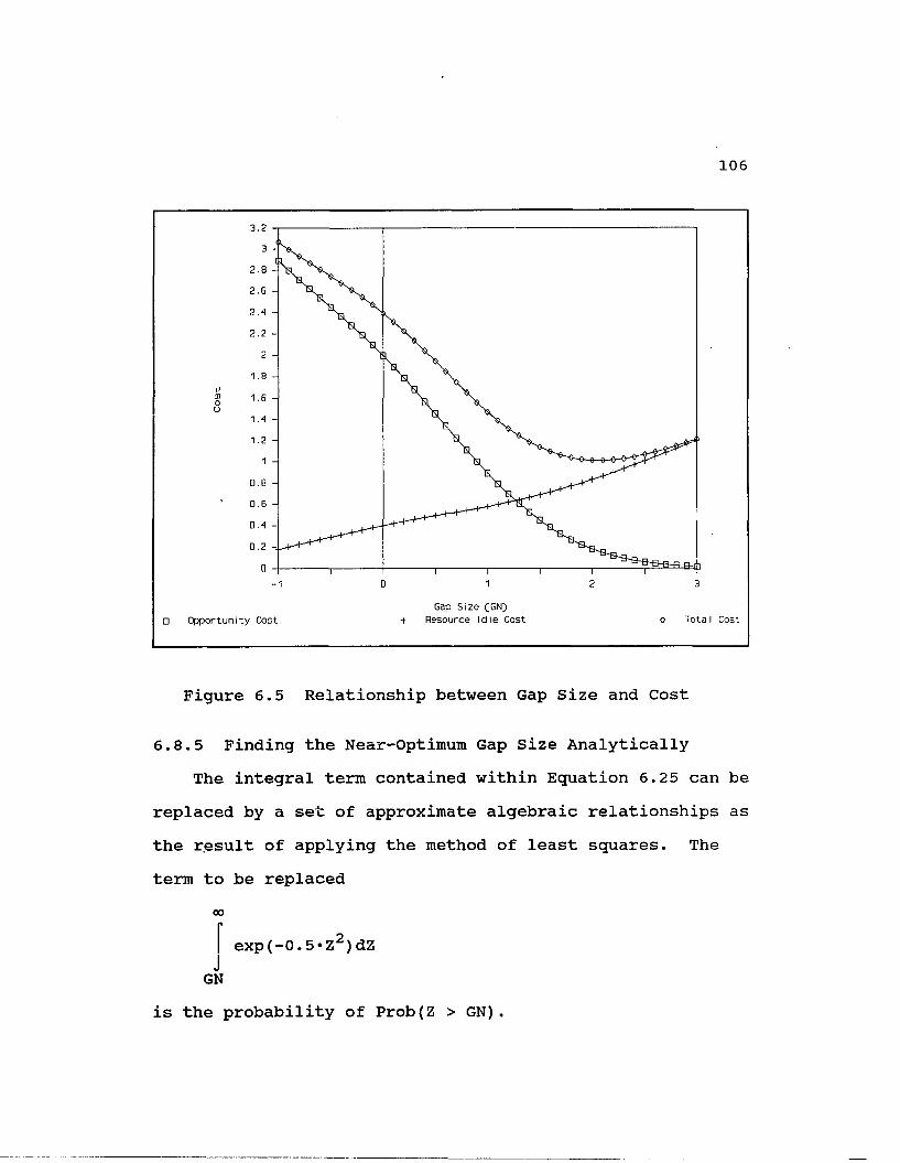
106

3

2

8

1

a

□ Opportunity CostGap Size CGN)

+ Resource Idle Cost Total cost

Figure 6.5 Relationship between Gap Size and Cost

6.8.5 Finding the Near-Optimum Gap Size AnalyticallyThe integral term contained within Equation 6.25 can be

replaced by a set of approximate algebraic relationships asthe result of applying the method of least squares. Theterm to be replaced

00»

exp(-0.5•Z2) dZGN

is the probability of Prob(Z > GN).

107The above expression is clearly dependent on the gap

size (GN). A table of values for the solution of the above expression, along with an associated range of gap sizes, is presented in Table 6.3. A plot of the tabulated valiles is shown in Figure 6.6. The form of the functional relationship can be approximated by a set of cosine and sine functions as follows:

oo

exp(-0.5*Z2)dZGN

« 0.5 + al*cos[Y*^/6] + a2 • sin[Y*7T/3] + a3 • sin[ Y-7T/1. 5]where Y = GN + 3.0,

7T = 3.1415927 andal, a2 and a3 are constants.

The constants, al, a2, and a3, may be found by shape fitting and the least squares method. Different sets of constants are inserted into the function over a range of GN values (i.e., a range of the domain GN is chosen to be between -3 and 3 because the probability of having a processing time variation which exceeds three times the standard deviation (3a) is only 0.0013). The function's results over the range of domain values are then plotted and compared to values of the exact solution. The least squares method is then employed to select the best parameter set.

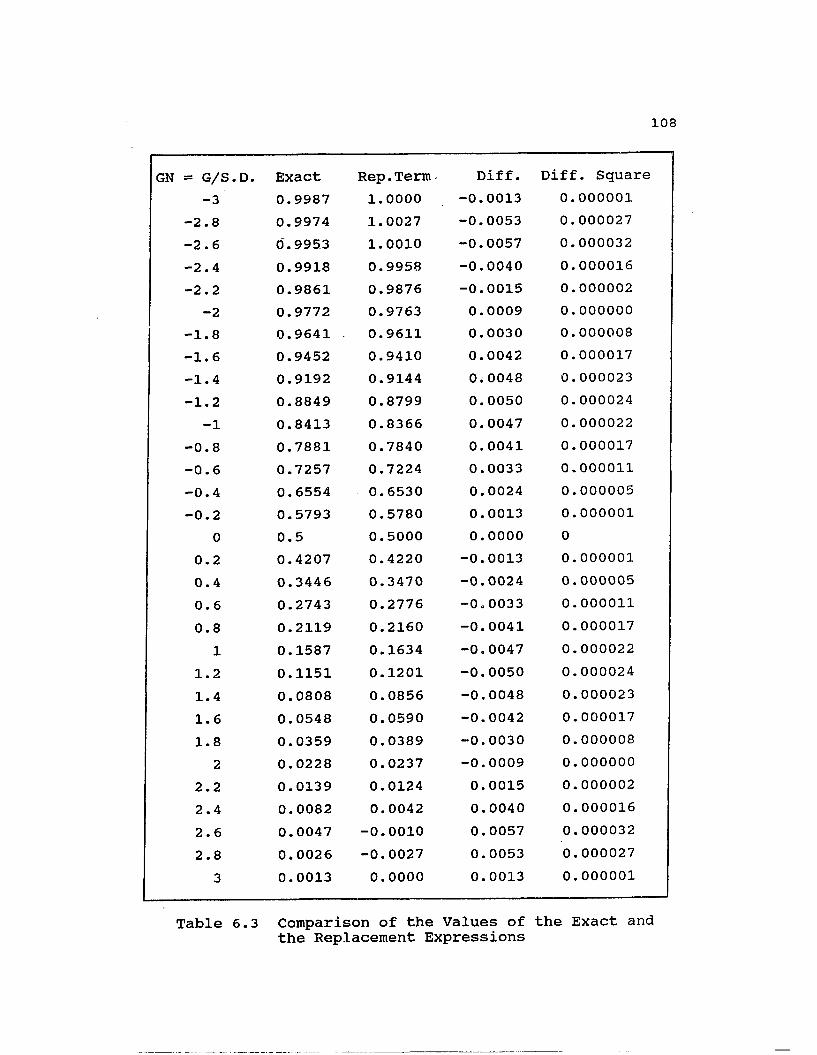
108

GN = G/S.D. Exact Rep.Term Diff. Diff. Square-3 0.9987 1.0000 -0.0013 0.000001

-2.8 0.9974 1.0027 -0.0053 0.000027-2.6 0.9953 1.0010 -0.0057 0.000032-2.4 0.9918 0.9958 -0.0040 0.000016-2.2 0.9861 0.9876 -0.0015 0.000002-2 0.9772 0.9763 0.0009 0.000000

-1.8 0.9641 0.9611 0.0030 0.000008-1.6 0.9452 0.9410 0.0042 0.000017-1.4 0.9192 0.9144 0.0048 0.000023-1.2 0.8849 0.8799 0.0050 0.000024

-1 0.8413 0.8366 0.0047 0.000022-0.8 0.7881 0.7840 0.0041 0.000017-0.6 0.7257 0.7224 0.0033 0.000011-0.4 0.6554 0.6530 0.0024 0.000005-0.2 0.5793 0.5780 0.0013 0.000001

0 0.5 0.5000 0.0000 00.2 0.4207 0.4220 -0.0013 0.0000010.4 0.3446 0.3470 -0.0024 0.0000050.6 0.2743 0.2776 -0.0033 0.0000110.8 0.2119 0.2160 -0.0041 0.000017

1 0.1587 0.1634 -0.0047 0.0000221.2 0.1151 0.1201 -0.0050 0.0000241.4 0.0808 0.0856 -0.0048 0.0000231.6 0.0548 0.0590 -0.0042 0.0000171.8 0.0359 0.0389 -0.0030 0.0000082 0.0228 0.0237 -0.0009 0.000000

2.2 0.0139 0.0124 0.0015 0.0000022.4 0.0082 0.0042 0.0040 0.0000162.6 0.0047 -0.0010 0.0057 0.0000322.8 0.0026 -0.0027 0.0053 0.000027

3 0.0013 0.0000 0.0013 0.000001

Table 6.3 Comparison of the Values of the Exact and the Replacement Expressions

109

-3Gap Size CGNJ

Replacement TermExact Term

Figure 6.6 Comparison between the Exact and the Replacement Expressions

Once the parameters have been estimated, values from the equation over the domain range (i.e., GN = -3.0,-2.9,...,-0.1, 0.0, 0.1,..., 2.9, 3.0) are compared to the exact solutions.

The parameter set found by this method can be used for any normally distributed processing time variation situation regardless of the value of the standard deviation. This is because the function domain is the normal gap size, GN, which has a standard deviation value

110of 1.0. For other standard deviation values, the gap size can easily be converted into standard form using the relation GN = G / a.

For a range of gap sizes between GN = -3 and GN = 3, the constant estimates are found to be al = 0.5, a2 = 0.075 and a3 = -0.025. A comparison of the replacement expression values and the actual values is shown in Table6.3 and Figure 6.6.

Parameter substitution allows the average total cost expression to be differentiated. By setting the result of the differentiation to zero, the optimum gap size equation can be reduced to a relatively simple algebraic expression.

■J*

Average Total Cost per Preventive Maintenance Job

a* exp(-0.5•(Y—3)2)(CPM + RC)

2.50663

a*(Y—3)+

2.50663

+ (0.075) *sin(Y-7r/3) + (-0.025) *sin(Y*7r/1.5) (6.26)

where Y GN + 3.0.

By setting A = a / 2.50663, B = RC + CPM and j3 = Y.7T/6, Equation 6.26 can be rewritten as follows:

IllAverage Total Cost per Preventive Maintenance Job

= A- B*exp(-0.5*(Y-3) ) + (RC - B/2)•(Y - 3)

- B* (Y-3) • (0. 5-COS/3 + 0. 075 • sin2/3 - 0. 025• sin4/3)

Differentiating the above equation with respect to the variable Y (i.e., Y = gap size (GN) + 3.0) results in the following expression:

d [total cost]d Y

= A-d exp(-0.5*(Y-3) ) d (Y - 3)

B + (RC --B/2)*---d Y d Y

- B*(Y-3)d (0.5*cos/3 + 0.075*sin2/3 - 0. 025 • sin4/3) » 'd Y

- B*(0.5*cos/3 + 0.075*sin2/3 - 0. 025• sin4/3) •-d (Y - 3)d Y

= A* B*exp(-0.5*(Y-3)d -0.5*(Y-3)d Y

+ (RC - B/2)

- B*(Y-3) •-sin/3 d/3 d2/3 d4/3-----*— + 0. 075*cos2/3*--- - 0.025*cos4/3*---

2 dY dY dY

- B* (0.5*cos/3 + 0.075*sin2/3 - 0. 025• sin4/0)

112

A* B* -(Y - 3)•exp(-0.5*(Y—3) ) + (RC/B -

- (Y—3)-sin/3 d/3 d/3-----•— + 0.15*cos2/3*— - 0.1'

2 dY dY

- (0.5*cos/8 + 0.075*sin2/3 - 0. 025• sin4/3)

d/3 d (Y*7T/6) 7TSince /3 = Y*tt/6, — = — = --

dY dY 6

d [total cost]d Y

= A*B*£ -(Y-3)*exp(—0.5*(Y—3) ) + (RC/B - 0

- (Y—3) • (-0. 2618 • sin/3 + 0. 07854 *cos2/3 - 0.

- (0.5*cos/3 + 0.075*sin2/3 - 0.025*sin4/3)= 0

where A = a / 2.50663, B = RC + CPM and /8 = Y*7T/6.

d/3COS4/3 • —

dY

= 0.5236, then

i.5)

0523 6 • COS4/3)

(6.27)

By solving Equation 6.27 for Y, the optimum gap size may be indirectly obtained, although solving for Y, or eventually GN, from Equation 6.27 is not possible algebraically. With

113the aid of the computer, however, the solution can be found

2numerically using a root finding algorithm.Comparison of the results obtained by applying the Van

Wijngaarden-Dekker-Brent numerical method and the previously discussed graphical method are shown in Table 6.4. Results from the two methods are not exactly the same, but they are certainly^similar. Considering that the results from the iterative method have an accuracy of ±0.05 and that the analytical method is based on an approximate expression of the probability function, the optimum gap sizes obtained from both methods are at least reasonably good.

Cases of CPM / RC

Optimum Gap Graphical Method

Size (GN)Analytical Method

7 2.20 2.125 2.10 1.993 1.90 1.771.5 1.40 1.401.25 1.30 1.280.75 -1.30 -1.320.5 -1.60 -1.560.25 -2.00 -1.90

Table 6.4 Comparison of Results from Graphical Method and Analytical Method

2The computer program coding of the Van Wijngaarden- Dekker-Brent Root Finding Method for solving Equation 6.27 is listed in Appendix B.

114

6.8.6 Limitation of the Analytical MethodThe root finding algorithm used to solve Equation 6.27

is only applicable for cases in which the ratio of the lost opportunity cost (CPM) to the resource cost (RC) is within the range of 0.15 and 7.5. This restriction is the result of the distortion of the replacement expression, which is employed in the curve fitting process, at both ends of the domain (i.e., the regions of GN close to 3.0 and -3.0). At the ends of the domain, the exact values of the probability terms are extremely small. This makes the differences between them and the replacement terms significant. For example, the exact value of Prob(Z > 2.6) is 0.0047, while the difference between the exact value and the replacement term value is 0.0057.

6.9 Master Scheduling Strategy for Preventive Maintenance Jobs

In this section, a master scheduling strategy for preventive maintenance jobs is set up based on the research described in this chapter. The master scheduling strategy is intended to serve as a guideline for preventive- maintenance-only scheduling. Figure 6.7 illustrates this strategy graphically. For each specific situation, an appropriate scheduling strategy is suggested.

115NO PROCESSING TIME VARIATION

For preventive maintenance jobs without processing time variation, scheduling can be done effectively by employing the Gantt Chart technique. It can be applied to situations of scheduling preventive maintenance jobs with or without lead time requirements. In such situations, no lost opportunity cost is incurred. The only cost involved is the resource cost. Section 6.4 discusses this situation in detail.

WITH PROCESSING TIME VARIATION, BUT WITH NO LEAD TIMEFor preventive maintenance jobs with processing time

variation but no lead time requirement, the one-job-at-a- time scheduling method discussed in Section 6.6 is most effective. By employing one-job-at-a-time scheduling, no lost opportunity cost is incurred while the resources are fully utilized.

WITH PROCESSING TIME VARIATION AND LEAD TIMEFor preventive maintenance jobs with processing time

variation and lead time requirements, scheduling becomes more complicated. There is no single method which is effective for all situations.

For a small lead time requirement, the one-job-at-a- time scheduling approach can be used. The major advantage of the one-job-at-a-time method is that it never incurs a lost opportunity cost. This is the result of all jobs

116being started at the planned time. However, some resource idle time is inevitable for this alternative. The resource idle time is the time that resources remain unused and in a waiting state during the lead time period. If the lead time period is short and the resource idle cost is low, the resource lost opportunity cost will also be low.

For a larger lead time requirement, the one-job-at-time scheduling method becomes less appropriate because of the increase in the resource lost opportunity cost. The effect of the lead time can be reduced by scheduling more than one job at a time. This alternative comes at a cost, however. The processing time variation of the first scheduled job can create a delayed starting situation for subsequently scheduled jobs. The planned time gap technique introduced in Section 6.7 can be used in this situation. However, it should be noted that the planned time gap technique is more appropriate than the one-job-at-time scheduling method only when the total cost incurred by the planned time gap technique is less than the resource lost opportunity cost incurred as a result of the resource waiting state during the lead time period in the one-job-at-a-time scheduling method.

It should also be noted that the planned time gap technique is based on the assumption that preventive jobs are not available for service before the scheduled starting time because of the online production circumstance. This

117assumption is not always appropriate. If a preventive job is available for maintenance service before its scheduled time, a scheduled negative time gap becomes unnecessary.

The purpose of a negative time gap is to avoid a resource idle period that may result from the negative processing time variation of the prior scheduled job. If the subsequently scheduled job can start immediately when the prior job finishes, no resources will be idle and consequently there will be no need for a negative time gap. Of course, a positive scheduled time gap is still necessary if a delayed start of the subsequently scheduled job causes a lost opportunity cost.

118

PM Alternative Scheduling Rules

No

No

No

Yes

o £ time gap quest1o n .* Length

is the

Re quIre Lead . T1me /

Ne xt Job S tar t Ea r 1 y

Process In T 1 me ,ya r 1 a t 1 o nS 1 m p 1 e .

Schedule One Job at a T 1 me

Exam1ne P r 1or/Current Work—orders

schedule Job with Positive Time Gap*

Ca1culate Positive or >Ne ga 1 1 ve T1me Ga p * and Schedule Job

Figure 6.7 Scheduling Strategy for Preventive Maintenance Jobs

CHAPTER 7MAINTENANCE SCHEDULING SYSTEM CONSIDERING BOTH EMERGENCY JOBS AND PREVENTIVE JOBS

The maintenance situation in which both emergency jobs and preventive maintenance jobs exist is more complicated than the situations analyzed in the previous two chapters. However, this maintenance situation commonly exists in reality and should be addressed. Two variations of this maintenance situation will be discussed. The first occurs when significant numbers of both emergency and preventive maintenance jobs exist. The second occurs when only one type of maintenance job is in the distinct majority. Possible approaches are introduced and discussed for each type of situation. However, because the alternatives are variations of situations already discussed previously, no mathematical treatment is presented.

7.1 Maintenance System with Significant Numbers of Both Emergency and Preventive Jobs

When the numbers of both emergency and preventive maintenance jobs are significant, the only solution which has proven effective in practice according to many maintenance schedulers (Casey 1976) is to divide maintenance resources and scheduling activities into two categories, preventive and emergency. Each category handles only one type of maintenance job and acts

119

120independently from the other. However, this division does not mean a complete separation between the two resource groups. Resource transfers between the two groups are still allowed periodically. For example, resource assigned to one group this week may be assigned to another group next week, while another resource may be reassigned based on day-to-day considerations.

There are several advantages to dividing a maintenance department into two separate groups. With two one-type maintenance groups, the strategies described in Chapters 5 and 6 can then be applied to each group. As has been shown, the application of independent group strategies is often more effective than the currently employed maintenance scheduling techniques. When both emergency and preventive maintenance activities are called for, the division of the maintenance staff is often justified because the numbers of both types of jobs are large enough to utilize resources allocated to both groups effectively. In a combined system which handles both emergency and preventive maintenance jobs, emergencies not only disrupt scheduled maintenance and thus disrupt the "control" of all maintenance activities, but they also result in an excessive waste of time and resources.

To successfully deploy both groups, however, the division of resources must be carefully done. The allocation of resources to each group should be performed

121systematically by using analytical methods (e.g., statistical forecasting techniques) and regularly reviewing maintenance activities to be sure that overstaffing or understaffing does not occur in either group.

7.2 Maintenance System with One Majority Job TypeThe division of the maintenance department into two

groups becomes nonsensical when there is only one major type of maintenance activity in the system. The resources allocated to the group that handles only small numbers of jobs are often underutilized, even when the smallest possible quantity of resources are assigned. The underutilization of resources becomes an even more serious problem when many types of resources are required to remain on stand by for the smaller group. Of course, the waste of resources increases as more resources stay in the idle state. Two separate situations are discussed for the maintenance system which has one major category of maintenance job, either an emergency activity majority or a preventive activity majority.

7.2.1 System with Emergency Jobs as the MajorityFor a system with emergency jobs as the clear majority

and a small number of preventive jobs, it may not be cost effective to allocate a group of resources to handle only the preventive jobs. There are two distinct alternative ways of handling this situation. One, the preventive jobs

122may be subcontracted. Because preventive jobs do not need service immediately, the contract-the-jobs-out practice is quite reasonable. This alternative also allows the in- house maintenance department to concentrate on emergency jobs only. Another reason this alternative may be appropriate is the obvious cost savings associated with having a smaller total maintenance crew.

Two, have the resources used to perform emergency jobs perform the service for the preventive jobs as well. This alternative is appropriate in two situations. The first situation is when the timing of preventive jobs does not need to be precise so that preventive jobs can be preempted by emergency jobs. The second situation occurs when the amount of resources required by preventive jobs is small compared to the total available resources. With a carefully set schedule, the assignment of a small portion of resources to preventive jobs may not affect the resource levels available to emergency jobs.

The major advantage of having a small number of preventive jobs performed by in-house maintenance personnel over the contract-out option is likely to be in terms of the cost. Since the resources are actually available for the emergency situation, no additional costs are incurred for the preventive tasks. However, the in-house option is not appropriate in all circumstances. In a tight or near fully utilized resource situation, the contract-out option

123may be a more appropriate alternative than adding an additional load of preventive jobs to an already heavily- loaded resource.

7.2.2 System with Preventive Jobs as the MajorityFor a system which rarely has an emergency job, having

a group of resources designated only to emergency jobs may obviously not be an effective approach. The preemptive option seems to be a better alternative. The preemptive strategy is to assign a small, specific group of maintenance resources to the resolution of emergency situations. Unlike the approach of having two independent maintenance groups as discussed in Section 7.1, a small group of resources may be assigned to do preemptable preventive jobs when there is no emergency need. With this arrangement, resources can be fully utilized and emergency jobs can be performed without delay.

7.3 Conclusion of Maintenance Scheduling Strategies Strategies for the maintenance scheduling system

considering both emergency jobs and preventive jobs described in this chapter are summarized in Table 7.1.

124

System Strategy

Both EM/PM common

Divide maintenance resources into 2 sections. One group handles EM jobs, while the other group handles PM jobs.

EmergencyMajority

A) Concentrate on EM; subcontract PM.B) Handle both types with carefully set

schedule.

PreventiveMajority

Resources needed for EM jobs are preemptable from PM jobs.

Table 7.1 Strategies for Maintenance Scheduling System Considering Both Emergency and Preventive Maintenance

CHAPTER 8CONCLUSION AND RECOMMENDATIONS

This research study reviewed current maintenance scheduling techniques in detail and discovered several shortcomings in the most widely used scheduling method, the priority index system. These shortcomings, as described in Chapter 3, indicated the need for a new maintenance scheduling system. Further study revealed that maintenance scheduling is a unique operation having several important differences from other classical scheduling models (e.g., the job shop) which have been addressed and studied previously by other researchers. These differences make the scheduling techniques recommended for those well-known situations inappropriate for maintenance scheduling. But there are also distinctly different categories of maintenance activities. Because of these differences, the maintenance system was divided into two subsystems for most of this research, maintenance systems which considered only emergency jobs and maintenance systems concerned only with preventive jobs. Each subsystem was analyzed. The details of these studies can be found in Chapters 5 and 6. As a result, a master scheduling strategy for each maintenance subsystem was presented. For a maintenance system concerned with both emergency and preventive jobs, Chapter

125

1267 suggested a number of strategies depending on the composition of jobs in the system.

Since many new factors are proposed for use in this new maintenance scheduling system and some currently used data are discarded, changes in the data requirements are required. Lost opportunity cost data must be developed for each possible emergency.maintenance activity. Lead time requirements, processing variation times, and start- earlier-than-scheduled-or-not data must be developed for each possible preventive maintenance activity. Neither the priority index nor the activity due date, key components in most current systems, are used directly in developing the maintenance activity schedule. The newly developed data become key components on the new maintenance scheduling system as shown in Figure 8.1.

Several new ideas and approaches to maintenance scheduling were introduced in this research study. Techniques from many areas, including operations research, mathematical modeling, statistics, numerical methods, and simulation, were employed.

Several additional research efforts are warranted to refine the ideas described in this dissertation. Models for maintenance systems with arrival and service processes other than the ones assumed are needed. Field studies which actually apply these techniques are, of course, warranted. Implementation and refinement of these

127scheduling techniques within a fully-formed maintenance information system and utilizing a maintenance scheduling expert system are also worthy of development.

Lost Opportunity Cost DBProcess Cost/T ime

116 500122 125

EM DatabaseActivity Processes Effected etc.

0001 0002

122116

227314

314• • ■■ - •

Emergency 0 0 0 2

EmergencyO O O l

Cs» lculateLost OpportunityCosts ...DetermineSchedule

Schedu1e

OOOl0 0 0 2

Figure 8.1 Uses of Database in the New Scheduling System

BIBLIOGRAPHY

Aurora, Ravinder Singh, Three-tier Scheduling. A Master Thesis in Industrial Engineering, Louisiana State University, Baton Rouge, Louisiana, (1987).

Baker, K. R., Introduction to Sequencing and Scheduling. John Wiley & Sons, New York, (1974).

Banks, Jerry and John S. Carson, II, Discrete-Event System Simulation. Prentice-Hall, Englewood Cliffs, New Jersey, (1984) .

Bodily, Samuel E., Modern Decision Making. McGraw-Hill, New York, (1985).

Brent, Richard P., Algorithms for Minimization without Derivatives. Prentice-Hall, Englewood Cliffs, New Jersey, (1973).

Buffa, Elwood S. and Jeffrey G. Miller, Production-Inventorv Systems Planning and Control. 3rd ed.. Irwin, Homewood, Illinois, (1979).

Burington, Richard Stevens, Handbook of MathematicalTables and Formulas. 5th ed.. McGraw-Hill, New York, (1973).

Casey, Peg, "Reorganization Provides For Planned andEmergency Maintenance", Maintenance Engineering, pp. 14-15, January, (1976).

Conway, Richard W., William L. Maxwell and Louis W. Miller, Theory of Scheduling. Addison-Wesley, Reading, Massachusetts, (1967).

Cooper, Robert B., Introduction to Queueing Theory. 2nd ed.. Elsevier North Holland, New York, (1981).

Czajkiewicz, Zbigniew, "Simulation Modeling for Heavy Industrial Equipment Maintenance", Computation & Industrial Engineering, vol.4, no.3, pp. 185-191,(1980).

Fishman, G.S., Principles of Discrete Event Simulation. John Wiley & Sons, New York, (1978).

Fry, Timothy D., Keong Leong and Terry R. Rakes, "Single Machine Scheduling: A Comparison of Two Solution Procedures", OMEGA. vol.15, July, pp. 277-283, (1987).

128

129Gross, Donald and Carl M. Harris, Fundamentals of Queueing

Theory. 2nd ed.. John Wiley & Sons, New York, (1985).Gupta, Sushil K. and Jerzy Kyparisis, "Single Machine

Scheduling Research", OMEGA. vol.15, no.3, pp. 207- 227, (1987).

Hax, Arnoldo C. and Dan Candea, Production and Inventory Management. Prentice-Hall, Englewood Cliffs, New Jersey, (1984).

Higgins, Lindley R., Maintenance Engineering Handbook.4th ed.. McGraw-Hill, New York, (1988).

Khemakavat, Nat, A Microcomputer-Aided Maintenance System with Emphasis on Plahning and Scheduling. A Master Thesis in Industrial Engineering, Louisiana State University, Baton Rouge, Louisiana, (1985) .

Law, Averill M. and W. David Kelton, Simulation Modeling and Analysis. McGraw-Hill, New York, (1982) .

Law, Averill M. and W. David Kelton, "Confidence Intervals for Steady-State Simulations, II: A Survey of Sequential Procedures", Management Science, vol.28, no.5, pp. 550-562, (1982).

McKay, Kenneth N., Frank R. Safayeni and John A. Buzacott, "Job-Shop Scheduling Theory: What Is Relevant", Interfaces. vol.18, no.4, pp. 84-90, (1988).

Mann, Lawrence, Jr., Maintenance Management. Rev. ed..D.C. Heath, Lexington, Massachusetts, (1983).

Niebel, Benjamin W., Engineering Maintenance Management. Marcel Dekker, New York, (1985).

O'Brien, James J., Scheduling Handbook. McGraw-Hill, New York, (1969).

Panwalkar, S.S. and W. Iskander, "A Survey of Scheduling Rules", Operations Research, vol.25, no.l, pp. 45-61, (1977) .

Pegden, C. Dennis, Introduction to SIMAN. Systems Modeling, State College, Pennsylvania, (1984) .

Press, William H., Brian P. Flannery, Saul A. Teukolsky and William T. Vetterling, Numerical Recipes. Cambridge University Press, New York, (1986).

130Scudder, Gary D. and Thomas R. Hoffmann, "The Use of Value-

Based Rules to Avoid Shop disruption", OMEGA. vol.14, pp. 259-265, (1986).

Scudder, Gary D. and Thomas R. Hoffmann, "The Use of Cost- Based Priorities in Random and Flow Shops", Journal of Operations Management, vol.7, no.2, pp. 217-232,(1987) .

Wittrock, Robert J., "An Adaptable Scheduling Algorithmfor Flexible Flow Lines", Operations Research, vol.36, pp. 445-454, (1988).

White, John A., J. W. Schmidt and G. K. Bennett, Analysis of Queueing Systems. Academic Press, New York, (1975).

APPENDIX A SIMULATION MODELS OF SCHEDULING TECHNIQUES

DESCRIBED IN CHAPTER 5

Five simulation models were created for testing purposes as described in Chapter 5. These simulation models were designed so that all models were tested under similar situations, throughout all simulation runs. This synchronization is essential for meaningful statistical comparisons. Simulation models were developed in SIMAN, a general purpose simulation language based on FORTRAN.SIMAN was created by C. Dennis Pegden and is available commercially on a range of computer systems. The models in this research were developed and run on an IBM PC- compatible microcomputer system.

A SIMAN simulation model consists of two major components, the system model and the experimental frame, plus optional user-coded FORTRAN subroutines. The program listings are included in the following sections. The program code is displayed in upper case form, while program comments are shown in lower case. Further information and explanation about SIMAN can be found in the text, Introduction to SIMAN. by C. Dennis Pegden (Pegden 1984).

131

A.1 Model of Proposed PlanSYSTEM MODEL

BEGIN;

Q1Q2

NX JOBEXITEND;

BEGIN;PROJECT,PROPOSED PLAN,NAT KHEMAKAVAT,12/16/88; DISCRETE,100,3,2;PARAMETERS:1,1.0:

2,0.8:3,0.0,100.0;

RESOURCES:1,SERVER;TALLIES:1,OPPORTUNITY COST:

2,WAITING TIME:3,TIME IN SYSTEM;

DSTAT:1,NR(1),SERVER UTIL:2,NQ(1),NO IN QUEUE;

REPLICATE,10,0,1100,YES,YES,100;OUTPUT:1,TAVG(1),11:

2,TAVG(2),12:3,TNUM(1),13;

END;USER-CODED FORTRAN SUBROUTINES

$STORAGE:2SUBROUTINE EVENT(JOB,N)CALL FINDJOB(JOB)RETURNEND

CREATE:EX(1,1):MARK(1);ASSIGN:A (2)=EX(2,2);ASSIGN:A (3)=UN(3,3);BRANCH,1:IF,NR(1) .EQ. 0,Q2:

ELSE,Q1;QUEUE,1:DETACH;QUEUE,2,1;SEIZE:SERVER;ASSIGN:A(3)=A(3)*(TNOW-A(l));TALLY:1,A(3);TALLY:2,INT(1);DELAY:A(2);RELEASE:SERVER; Finish serviceBRANCH,l:IF,NQ(l) .GT. 0,NXJOB:

ELSE,EXIT;EVENT:1;REMOVE:A(2),1,Q2; Select next jobTALLY:3,INT(1):DISPOSE;

EXPERIMENTAL FRAME

Job arrival Processing time Opportunity cost

Waiting queue Start service

133

SUBROUTINE FINDJOB(JOB)REAL COST(2)COMMON/SIM/D(50),DL(50),S(50),SL(50),X(50),DTNOW, 1TNOW,TFIN,J,NRUN NOINQ = NQ(1)IF (NOINQ .EQ. 1) THEN

J = 1 ENDIFIF (NOINQ .EQ. 2) THEN

COST(1) = A (LFR(1), 2)*A (LLR(1),3)COST(2) = A (LLR(1),2)*A (LFR(1),3)IF (COST(1) .LT. COST(2)) THEN

J = 1 ELSE

J = 2 ENDIF

ENDIFIF (NOINQ .GE. 3) THEN

JS = 1 JH = 1 LOC = LFR(1)SPT = A(LOC,2)HWF = A(LOC,3)HPT = SPT DO 10 K=2,NOINQ

LOC = LSUCC(LOC)PT = A (LOC,2)CO = A(LOC,3)IF (PT .LT. SPT) THEN

SPT = PT JS = K

ENDIFIF (CO .GT. HWF) THEN

HWF = CO HPT = PT JH = K

ENDIF 10 CONTINUE

C compare costsCSPT =0.0 CHWF =0.0 DO 15 K=l,NOINQ

IF (K .EQ. 1) THEN LOC = LFR(1)

ELSELOC = LSUCC(LOC)

ENDIFIF (JS .NE. K) THEN

CSPT = CSPT + A(LOC,3)*SPT ENDIFIF (JH .NE. K) THEN

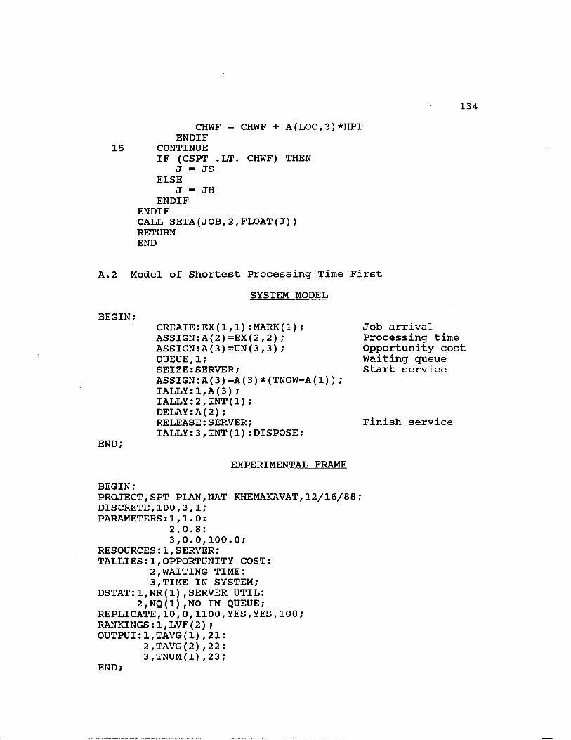
134CHWF = CHWF + A (LOC,3)*HPT

ENDIF 15 CONTINUE

IF (CSPT .LT. CHWF) THEN J = JS

ELSEJ = JH

ENDIF ENDIFCALL SETA(JOB,2,FLOAT(J))RETURNEND

A.2 Model of Shortest Processing Time FirstSYSTEM MODEL

BEGIN;CREATE:EX(1,1):MARK(1);ASSIGN:A(2)=EX(2,2);ASSIGN:A (3)=UN(3,3);QUEUE,1;SEIZE:SERVER;ASSIGN:A(3)=A(3)*(TNOW—A(l));TALLY:1,A(3);TALLY:2,INT(1);DELAY:A (2);RELEASE:SERVER;TALLY:3,INT(1):DISPOSE;

END;EXPERIMENTAL FRAME

BEGIN;PROJECT,SPT PLAN,NAT KHEMAKAVAT,12/16/88; DISCRETE,100,3,1;PARAMETERS:1,1.0:

2,0.8:3,0.0,100.0;

RESOURCES:1,SERVER;TALLIES:1,OPPORTUNITY COST:

2,WAITING TIME:3,TIME IN SYSTEM;

DSTAT:1,NR(1),SERVER UTIL:2,NQ(1),NO IN QUEUE;

REPLICATE,10,0,1100,YES,YES,100;RANKINGS:1,LVF(2);OUTPUT:1,TAVG(1),21:

2,TAVG(2),22:3,TNUM(1),23;

END;

Job arrival Processing time Opportunity cost Waiting queue Start service

Finish service

135

A.3 Model of Highest Opportunity Cost FirstSYSTEM MODEL

BEGIN;

END;

CREATE:EX(1,1):MARK(1); ASSIGN:A (2)=EX(2,2);ASSIGN:A (3)=UN(3,3);QUEUE,1;SEIZE;SERVER;ASSIGN:A(3)=A(3)*(TNOW-A(l)); TALLY:1,A(3);TALLY:2,INT(1);DELAY:A (2);RELEASE:SERVER;TALLY:3,INT(1):DISPOSE;

Job arrival Processing time Opportunity cost Waiting queue Start service

Finish service

EXPERIMENTAL FRAMEBEGIN;PROJECT,HOCF PLAN,NAT KHEMAKAVAT,12/16/38; DISCRETE,100,3,1;PARAMETERS:1,1.0:

2,0.8:3,0.0,100.0;

RESOURCES:1,SERVER;TALLIES:1,OPPORTUNITY COST:

2,WAITING TIME:3,TIME IN SYSTEM;

DSTAT:1,NR(1),SERVER UTIL:2,NQ(1),NO IN QUEUE;

REPLICATE,10,0,1100,YES,YES,100;RANKINGS:1,HVF(3);OUTPUT:1,TAVG(1),31:

2,TAVG(2),32:3,TNUM(1),33;

END;I

136A.4 Model of First-in First-out

SYSTEM MODELBEGIN?

CREATE:EX(1,1):MARK(1)?ASSIGN:A (2)=EX(2,2);ASSIGN:A (3)=UN(3,3)?QUEUE,1?SEIZE:SERVER;ASSIGN:A(3)=A(3)*(TNOW—A(l))? TALLY:1,A(3);TALLY:2,INT(1);DELAY:A(2);RELEASE:SERVER;TALLY:3,INT(1):DISPOSE;

Job arrival Processing time Opportunity cost Waiting queue Start service

Finish serviceEND;

EXPERIMENTAL FRAMEBEGIN;PROJECT,FIFO PLAN,NAT KHEMAKAVAT,12/16/88; DISCRETE,100,3,1;PARAMETERS:1,1.0:

2,0.8:3,0.0,100.0;

RESOURCES:1,SERVER;TALLIES:1,OPPORTUNITY COST:

2,WAITING TIME:3,TIME IN SYSTEM;

DSTAT:1,NR(1),SERVER UTIL:2,NQ(1),NO IN QUEUE;

REPLICATE,10,0,1100,YES,YES,100;OUTPUT:1,TAVG(1),41:

2,TAVG(2),42:3,TNUM(1),43;

END;

137A.5 Model of Method of One Step Trial

SYSTEM MODELBEGIN?

CREATE:EX(1,1):MARK(1);ASSIGN:A(2)=EX(2,2);ASSIGN:A(3)=UN(3,3);BRANCH,1:IF,NR(1) .EQ. 0,Q2:

ELSE,Q1;Q1 QUEUE,1:DETACH;Q2 QUEUE,2,1?

SEIZE:SERVER?ASSIGN:A(3)=A(3)*(TNOW-A(l));TALLY:1,A (3);TALLY:2,INT(1);DELAY:A (2)?RELEASE:SERVER;BRANCH,1:IF,NQ(1) .GT. O.NXJOB:

ELSE,EXIT;NXJOB EVENT:1;

REMOVE:A (2),1,Q2?EXIT TALLY:3,INT(1):DISPOSE;

END;EXPERIMENTAL FRAME

BEGIN?PROJECT,TRIAL METHOD,NAT KHEMAKAVAT,12/16/88; DISCRETE,100,3,2;PARAMETERS:1,1.0:

2,0.8:3,0.0,100.0;

RESOURCES:1,SERVER;TALLIES:1,OPPORTUNITY COST:

2,WAITING TIME:3,TIME IN SYSTEM;

DSTAT:1,NR(1),SERVER UTIL:2,NQ(1),NO IN QUEUE;

REPLICATE,10,0,1100,YES,YES,100;OUTPUT:1,TAVG(1),51:

2,TAVG(2),52:3,TNUM(1),53?

END;USER-CODED FORTRAN SUBROUTINES

$STORAGE:2SUBROUTINE EVENT(JOB,N)CALL FINDJOB(JOB)RETURNEND

Job arrival Processing time Opportunity cost

Waiting queue Start service

Finish service

Select next job

138

SUBROUTINE FINDJOB(JOB)INTEGER LOC(50)COMMON/SIM/D(50),DL(50),S(50),SL(50),X(50),DTNOW, 1TNOW,TFIN,J,NRUN NOINQ = NQ(1)IF (NOINQ .EQ. 1) THEN

IP = 1 ENDIFIF (NOINQ .GT. 1) THEN

DO 20 K=l,NOINQIF (K .EQ. 1) THEN

LOCATION = LFR(l)ELSE

LOCATION = LSUCC(LOCATION)ENDIFLOC(K) = LOCATION

20 CONTINUE IP = 0COSTP = l.E+10 DO 30 K=l,NOINQ

COST =0.0 PROT = A(LOC(K) ,2)IF (K .NE. 1) THEN

DO 34 KA=1,K-lCOST = COST + PROT*A(LOC(KA),3)

34 CONTINUEENDIFIF (K .NE. NOINQ) THEN

DO 36 KA=K+1,NOINQCOST = COST + PROT*A(LOC(KA),3)

36 CONTINUEENDIFIF (COST .LT. COSTP) THEN

IP = K COSTP = COST

ENDIF 30 CONTINUE

ENDIFCALL SETA(JOB,2,FLOAT(IP))RETURNEND

APPENDIX B VAN WIJNGAARDEN-DEKKER-BRENT

ROOT FINDING ALGORITHM

The major task of a root finding algorithm is to find all possible solutions or roots of a function which is in the form of f(x) = 0. There are many root finding algorithms available, but no root finding algorithm is perfect for all situations. For our need, which was to solve Equation 6.27, a general one-dimensional function (i.e., only one independent variable to be solved), the Van Wijngaarden-Dekker-Brent method was recommended by Press and Associates (Press 1986). The reason is that it is guaranteed (by Brent) to converge, so long as the function can be evaluated within the initial interval known to contain a root.

A computer program, written in Turbo Pacal Version 4.0, employed the Van Wijingaarden-Dekker-Brent method to solve Equation 6.27 for the optimum gap size. The function Zbrent included in the program is taken from Numerical Recipes by Press and Associates.

139

140

PROGRAM Optimumgap;VAR

cpm, rc, ac, be, y, sd, oppy, oppgn : real; lowbound, upbound, acc : real;

FUNCTION Fy (y : real) : real;(* a function provides the value of equation (6.27) for

a given value, y. *)VAR

beta : real;BEGIN { function Fy }

beta := y*Pi/6.0;Fy := ac*bc*(-(y-3)*exp(-0.5*sqr(y-3)) + (rc/bc - 0.5)

- (y-3)*(sin(beta)*(-Pi/12.0)+ 0.075*Pi*cos(2.0*beta)/3.0- 0.025*Pi*2.0*cos(4.0*beta)/3.0)- (0.5*cos(beta) + 0.075*sin(2.0*beta)- 0.025*sin(4.0*beta)));

END; { function Fy }FUNCTION Zbrent (xl, x2, tol ; real) ; real;

(* Using Van Wijngaarden-Dekker-Brent method, find the root of a function Fy known to lie between xl and x2.The root, returned as Zbrent, will be returned untilits accuracy is tol. *)

LABEL 99;CONST

itmax = 100; eps = 3.Oe-8;

VARa, b, c, d, e : real; mini, min2, min ; real; fa, fb, fc, p, q, r : real; s, toli, xm : real; iter : integer;

BEGIN { function Zbrent }a := xl; b ; = x2 ; fa := fx(a); fb := fx(b);if (fb*fa > 0.0) then begin { if 1 }

writeln('pause in routine ZBRENT1); writeln(1 root must be bracketed'); readlnend; { if 1 }

fc := fb;for iter := 1 to itmax do begin { for )

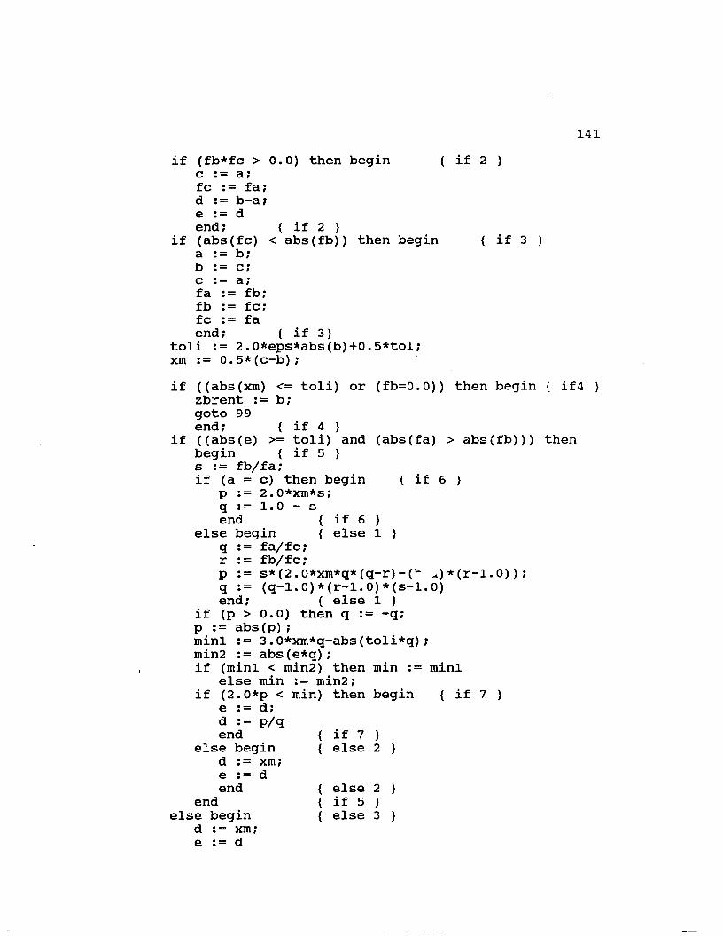
141if (fb*fc > 0.0) then begin { if 2 }

c : = a; fc := fa; d := b-a; e := dend; { if 2 }

if (abs(fc) < abs(fb)) then begin { if 3 ) a := b; b : = c; c : = a; fa := fb; fb := fc; fc := faend; { if 3}

toli := 2.0*eps*abs(b)+0.5*tol; xm := 0.5*(c-b);if ((abs(xm) <= toli) or (fb=0.0)) then begin { if4 )

zbrent := b ; goto 99end; { if 4 }

if ((abs(e) >= toli) and (abs(fa) > abs(fb))) thenbegin { if 5 }s := fb/fa;if (a = c) then begin { if 6 }

p ;= 2.0*xm*s; q := 1.0 - s end { if 6 )

else begin { else 1 }q ;= fa/fc; r := fb/fc;p := s*(2.0*xm*q*(q-r)-(u .*) * (r-1. 0)) ; q := (q-1.0)*(r-1.0)*(s-1.0) end; { else 1 )

if (p > 0.0) then q := -q; p := abs(p);mini := 3.0*xm*q-abs(toli*q); min2 ;= abs(e*q); if (mini < min2) then min ;= mini

else min := min2; if (2.0*p < min) then begin { if 7 }

e : = d; d := p/qend { if 7 }

else begin { else 2 }d ;= xm; e := dend { else 2 }

end { if 5 )else begin { else 3 }

d ;= xm; e ;= d

end; { else 3 }a := b; fa ;= fb;if (abs(d) > toli) then begin { if 8 }

b := b+dend { if 8 }

else begin { else 4 )if (xm > 0) then begin { if 9 )

b := b+abs(toli) end { if 9 )

else begin { else 5 )b := b-abs(toli) end { else 5 }

end; { else 4 )fb := fx(b) end; { for }

writeln('pause in routine ZBRENT1);writeln('maximum number of iterations exceed') readln;Zbrent := b;

99: end; { function Zbrent }begin { program Optimumgap }

write('Enter CPM : '); readln(cpm); write('Enter RC : ');readln(rc);write('Enter S.D. of processing time variation readln(sd);ac := sd / sqrt(2.0*Pi); be := rc + cpm; lowbound := 0.0; upbound := 6.0; acc:= 0.000001;oppy := zbrent(lowbound,upbound,acc); oppgn := oppy - 3.0;writeln('Optimum gap size is ',oppgn:10:4);

end. { program Optimumgap }

VITA

Nat Khemakavat was born in Bangkok, Thailand on January 25, 1959. He received his elementary and high school education at Assumption College in Bangkok, Thailand. In 1978, he enrolled in Chulalongkorn University, Bangkok, and received a Bachelor of Science degree in Mechanical Engineering in March of 1982. After graduation, he was employed as an engineer by ESSO Standard Thailand Ltd. in Bangkok. In January 1984, he enrolled in the graduate school at Louisiana State University and received a Master of Science degree in Industrial Engineering in December of 1985. He continued his graduate study at Louisiana State University and is presently a candidate for a Doctor of Philosophy degree in Engineering Science.

143

DOCTORAL EXAMINATION AND DISSERTATION REPORT

Candidate: N at Khemakavat

Major Field: E n g in e e r in g S c ie n c e

Title o f Dissertation: E v a l u a t i o n a n d I m p r o v e m e n t o f M a i n t e n a n c e S c h e d u l i n g T e c h n i q u e s

Approved:

Major Professor and Chairman

-6Dean of the Graduate

EXAMINING COMMITTEE.

’l O K U t D / n . ; ' .

-Q

-A-v.At v v...

£

Date of Examination:

F e b r u a r y 1 5 , 1 9 8 9