1

Evaluation and Exploration of Next Generation Systems for Applicability and

Performance (Volodymyr Kindratenko, Guochun Shi)

1 Summary

We have ported image characterization algorithm implemented in doc2learn application to the

Graphics Processing Unit (GPU) platform using both CUDA C targeting NVIDIA GPUs and

OpenCL targeting NVIDIA and AMD GPU architectures. We also implemented doc2learn

image analysis algorithm in C targeting microprocessor architecture. Our conclusion is that

doc2learn image processing part can be accelerated up to 4 times using NVIDIA GTX 480 GPU,

but 1) the speedup depends on the image size and 2) other parts of doc2lear application dominate

the execution time.

2 Preliminaries

Doc2learn implements algorithms for computing probability density functions for text, image,

and vector graphics objects embedded into PDF files. Specifically, non-parametric probability

density function estimation techniques are implemented that require computing a histogram of

frequencies of occurrence of all values in a particular object, e.g., image or text. The computed

probability density functions (histograms) form the feature vector which can be used for

measuring the similarity between pairs of images.

Figure 1. Doc2learn execution profile using has.PDF as an example. Pie chart on the left shows time distribution of

the entire application. Pie chart on the right shows time distribution of the data processing part, which is 25% of the

overall application execution time.

Application profiling of doc2learn SVN revision 760 on has.pdf file (one of test cases) reveals

that about 25% of the overall time is spent on the probability density function computation

(Figure 1, left) most of which is spent on the image analysis (Figure 1, right). This time

distribution is typical for documents containing many images.

2

Doc2learn is written in Java. Java code is executed by a virtual machine that executes on top of

the actual hardware (microprocessor). Java virtual machine isolates many of the performance-

enhancing features of the underlying hardware, such as vector units, thus potentially not allowing

to fully utilize the capabilities of modern microprocessors without explicitly programming for

them. The main goal of this study is to investigate how the execution of the probability

density function computation for images can be improved on modern microprocessor

architectures and GPUs. We specifically target image analysis part of the doc2learn

application because it is perceived to be the most data-intensive and time-consuming part of the

computation for documents that contain either a lot of images or large-size images.

2.1 Doc2learn image characterization algorithm

Doc2learn implements a non-parametric probability density function estimation technique which

is based on the computation of a histogram of frequencies of occurrence of pixels of different

colors in an image. Most significant bits of red, green, and blue components (and optionally

alpha channel when present) of each image pixel are used as indexes of a 3D array that holds the

histogram. This algorithm is an improvement over the histogram computation algorithm used in

earlier versions of doc2learn. Instead of building a histogram consisting of all color values

present in the image, a highly reduced histogram is computed, resulting in a very significant

(over an order of magnitude) reduction of the computation time.

Figure 2 contains the Java source code for probability density function estimation taken from the

original doc2learn implementation.

// compute histogram for image

int pix, red, green, blue;

for (int r = 0; r < bi.getHeight(); r++ ) {

for (int c = 0; c < bi.getWidth(); c++ ) {

pix = bi.getRGB(c, r);

red = ((pix >> 16) & 0xff) / size;

green = ((pix >> 8) & 0xff) / size;

blue = (pix & 0xff) / size;

histogram[red][green][blue]++;

}

}

Figure 2. Original Java implementation of the image probability density function computation.

2.2 Hardware platforms used in this study

Two computer systems have been used in this study: 1) Intel based with Fermi GTX 480 GPU

and 2) AMD based with ATI Radeon 5870 GPU. Table 1 contains technical characteristics of

both systems. If not explicitly said, results reported in this report, such as the application profile

shown above, were obtained on the Intel-based system which was found to be better performing.

Intel-based system AMD-based system

Processor 3.3 GHz single 4-core Core i7 2.8 GHz dual 6-core Istanbul

Memory 24 GB DDR3 32 GB DDR2 GPU NVIDIA GeForce GTX 480 ATI Radeon HD5870

PCIe interface 2.0 2.0 Table 1. Characteristics of the two computer systems used in this study.

3

2.3 GPU kernel offload programming model

Figure 3, left, shows a typical architecture of a GPU-enabled computing system. A GPU is

added to the conventional multi-core system via the Peripheral interface (PCIe). GPU card

contains its own memory (referred to as the device memory)

Figure 3. left: Architecture of a typical GPU-based computing system. Right: Typical sequence of steps nessesary

to implement kernel offload to the GPU.

Executing a computational kernel on the GPU involves several steps, as shown in Figure 3, right.

First, a GPU device is discovered and configured. This step is implicitly performed by the

NVIDIA CUDA SDK when a call to CUDA SDK is made. However, when using OpenCL, it is

programmer’s responsibility to perform this step explicitly. Second, data from the host (image

data in our case) is transferred to the memory accessible by the GPU (device memory). This

transfer occurs over the PCIe interface and adds to the overall execution time. Next, the actual

GPU kernel is invoked. When the kernel execution finishes, computed results are transferred

from the device memory to the host memory. The programming model that implements these

steps is referred to as kernel offload model because the execution of (presumably)

computationally intensive portion of the code is offloaded to the GPU for accelerated execution.

2.4 Performance measurements

When comparing performance of the code executed on the GPU with the original Java code

executed on the host by the Java virtual machine, it is important to measure and report the

execution time that includes all the overheads associated with the use of a particular computing

hardware. In this study we report execution time measured within the Java code. In case of the

pure Java implementation, the time measured reflects the time spent executing the computation

by the Java virtual machine (Figure 4, top). In case of the C port of the computational kernel, the

time measured includes the overhead associated with calling a C function from Java, execution

of the C function, and the overhead of copying results computed by the C function to the Java

data structures (Figure 4, middle). In case of the GPU implementation, the measured time

reflects all the overheads associated with the invocation of a C function from Java virtual

4

machine, overheads due to the data transfer from the host memory to the device memory, GPU

kernel execution time, and the device to host data transfer time (Figure 4, bottom).

Figure 4. Measured application time includes all the overheads involved in using the underlying hardware.

3 Technical activities, findings, and results

3.1 Java code optimization

Further profiling of the doc2learn code shown in Figure 2 revealed that bi.getRGB(c, r)

function is responsible for the vast majority of the time spent in this code. getRGB function

performs color space conversion, if needed. But in the majority of cases images are stored in the

RGB format and such color space conversion is unnecessary. Therefore, for images that are

already in RGB color space we can eliminate this call as shown in Figure 5. This simple

optimization improves the execution of the image probability density function estimation by a

factor of ~6, reducing the image processing part for has.pdf example from 1,655 ms to 274 ms.

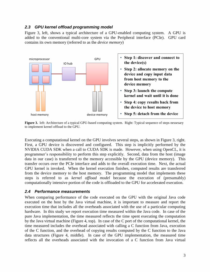
In the rest of this study we use this updated code for performance comparison analysis. Figure 6

contains updated application execution profile shown in Figure 1 after this code optimization is

applied.

// compute histogram for image

int red, green, blue;

byte[] data = ((DataBufferByte)bi.getRaster().getDataBuffer()).getData();

for (int i =0; i < data.length; i+=3){

red =(data[i] & 0xff) / size;

green = (data[i+1] & 0xff)/ size;

blue = (data[i+2] & 0xff) / size;

histogram[red][green][blue]++;

}

Figure 5. Improved Java implementation of the image probability density function computation.

C function executed on the CPU host

host to device

data transfer

device to host

data transfer

GPU kernel

execution

Original Java implementation of the computational kernel

Call C function Copy results

Call C function Copy results

GPU time

CPU time

actual application time

5

Figure 6. Doc2learn execution profile when using the improved Java image analysis code.

3.2 Java to C port

Java-C interface is implemented using Java Native Interface (JNI). On the Java side of the

application, we only need to obtain a pointer to the image data and pass it to the C subroutine

which is compiled using a C compiler, such as ICC or GCC. Figure 7 shows how the C

subroutine is called in place of the code shown in Figure 5, Figure 8 shows C implementation

that corresponds to Java implementation shown in Figure 4.

int bincolor = (int) Math.pow(BINS, 1.0 / 3.0);

int size = 256 / bincolor;

int[][][] histogram = new int[bincolor][bincolor][bincolor];

int pix, red, green, blue;

byte[] data = ((DataBufferByte)bi.getRaster().getDataBuffer()).getData();

ImageHistCPU ihg = new ImageHistCPU();

int[] hist_from_cpu = ihg.computeImageHist(data); // compute histogram in C function

for(red = 0; red < bincolor ; red++) { // copy results back to Java storage

for(green = 0; green < bincolor ; green++) {

for(blue = 0; blue < bincolor ; blue++) {

histogram[red][green][blue]=hist_from_cpu[red*bincolor*bincolor+green*bincolor+blue];

}

}

}

Figure 7. Source code showing how histogram computation is replaced with a call to a C function.

Execution time of the Java version of this code using has.pdf data file is 274 ms. Execution time

of the corresponding C implementation compiled with GCC compiler using highest level of

optimization (-O3) is 109 ms as measured on the Java side of the application, or 2.5 times faster

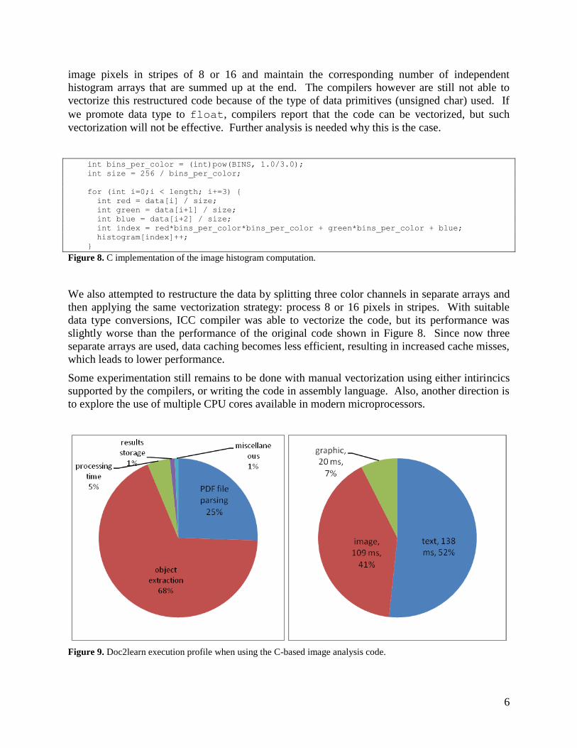
than the native Java implementation. Updated application profile is shown in Figure 9.

Note that neither GCC nor ICC compilers are able to vectorize the code due to the data

dependency on histogram[]. The code, however, can be restructured to process several

6

image pixels in stripes of 8 or 16 and maintain the corresponding number of independent

histogram arrays that are summed up at the end. The compilers however are still not able to

vectorize this restructured code because of the type of data primitives (unsigned char) used. If

we promote data type to float, compilers report that the code can be vectorized, but such

vectorization will not be effective. Further analysis is needed why this is the case.

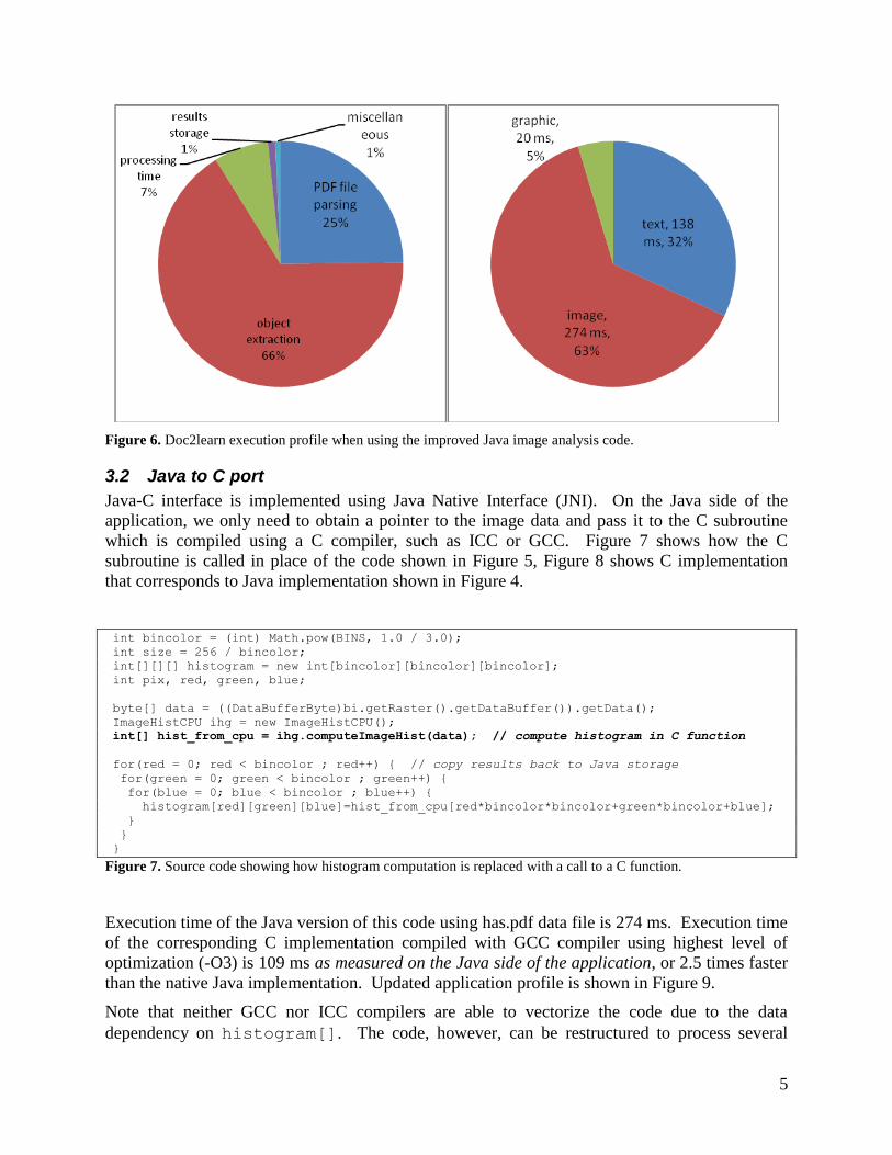
int bins_per_color = (int)pow(BINS, 1.0/3.0);

int size = 256 / bins_per_color;

for (int i=0;i < length; i+=3) {

int red = data[i] / size;

int green = data[i+1] / size;

int blue = data[i+2] / size;

int index = red*bins_per_color*bins_per_color + green*bins_per_color + blue;

histogram[index]++;

}

Figure 8. C implementation of the image histogram computation.

We also attempted to restructure the data by splitting three color channels in separate arrays and

then applying the same vectorization strategy: process 8 or 16 pixels in stripes. With suitable

data type conversions, ICC compiler was able to vectorize the code, but its performance was

slightly worse than the performance of the original code shown in Figure 8. Since now three

separate arrays are used, data caching becomes less efficient, resulting in increased cache misses,

which leads to lower performance.

Some experimentation still remains to be done with manual vectorization using either intirincics

supported by the compilers, or writing the code in assembly language. Also, another direction is

to explore the use of multiple CPU cores available in modern microprocessors.

Figure 9. Doc2learn execution profile when using the C-based image analysis code.

7

3.3 CUDA C implementation

CUDA C NVIDIA GPU implementation follows the traditional kernel offload programming

model described earlier. A C function is invoked from the Java application. The C function

copies image data from the host memory to the device memory, calls the kernel GPU function

and waits until it completes, copies results from the device memory to the host memory, and

returns the execution control to the Java application. The GPU kernel function was initially

implemented with each thread block computing its own copy of the histogram stored in the

shared memory. Multiple copies of the histograms are then merged at the end. Source code of

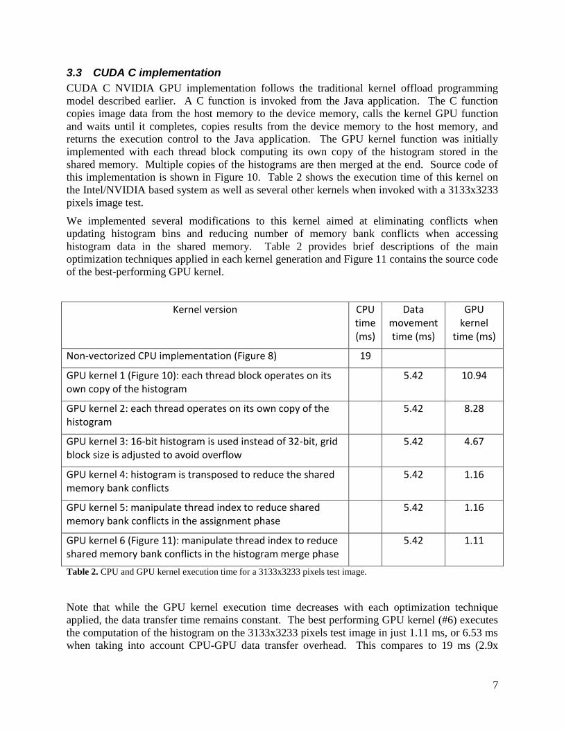
this implementation is shown in Figure 10. Table 2 shows the execution time of this kernel on

the Intel/NVIDIA based system as well as several other kernels when invoked with a 3133x3233

pixels image test.

We implemented several modifications to this kernel aimed at eliminating conflicts when

updating histogram bins and reducing number of memory bank conflicts when accessing

histogram data in the shared memory. Table 2 provides brief descriptions of the main

optimization techniques applied in each kernel generation and Figure 11 contains the source code

of the best-performing GPU kernel.

Kernel version CPU time (ms)

Data movement time (ms)

GPU kernel

time (ms)

Non-vectorized CPU implementation (Figure 8) 19

GPU kernel 1 (Figure 10): each thread block operates on its own copy of the histogram

5.42 10.94

GPU kernel 2: each thread operates on its own copy of the histogram

5.42 8.28

GPU kernel 3: 16-bit histogram is used instead of 32-bit, grid block size is adjusted to avoid overflow

5.42 4.67

GPU kernel 4: histogram is transposed to reduce the shared memory bank conflicts

5.42 1.16

GPU kernel 5: manipulate thread index to reduce shared memory bank conflicts in the assignment phase

5.42 1.16

GPU kernel 6 (Figure 11): manipulate thread index to reduce shared memory bank conflicts in the histogram merge phase

5.42 1.11

Table 2. CPU and GPU kernel execution time for a 3133x3233 pixels test image.

Note that while the GPU kernel execution time decreases with each optimization technique

applied, the data transfer time remains constant. The best performing GPU kernel (#6) executes

the computation of the histogram on the 3133x3233 pixels test image in just 1.11 ms, or 6.53 ms

when taking into account CPU-GPU data transfer overhead. This compares to 19 ms (2.9x

8

speedup) when compared to the C implementation or to 39 ms when taking into account the

additional 20 ms overhead due to the C function invocation from doc2learn Java program and

corresponding data fetch in the C program necessary to access image data (JNI overhead). Thus,

taking into account all overheads, the overall speedup of the GPU implementation compared to

the C-based CPU implementation as seen by the end user is only ~1.5x.

__global__ void histogramKernel1(void* imagedata, unsigned int n, unsigned int* result)

{

__shared__ unsigned int hist[64];

int i, idx = blockIdx.x*blockDim.x + threadIdx.x;

if (threadIdx.x < 64)

hist[threadIdx.x] = 0;

__syncthreads();

int total_num_threads= blockDim.x * gridDim.x;

int num_pixels = n /3 ;

unsigned char* bytedata = (unsigned char*)imagedata;

for (i =idx; i< num_pixels;i += total_num_threads) {

unsigned char r = bytedata[3*i];

unsigned char g = bytedata[3*i + 1];

unsigned char b = bytedata[3*i + 2];

r = r >> 6;

g = g >> 6;

b = b >> 6;

int bin_idx = (r << 4) + (g << 2) + b;

atomicAdd( &hist[bin_idx], 1);

}

__syncthreads();

if(threadIdx.x < 64)

result[blockIdx.x * REAL_BINS + threadIdx.x] = hist[threadIdx.x];

return;

}

Figure 10. Initial GPU Kernel implementation (kernel 1 in Table 2).

We also tried to overlap image data transfer with the GPU computation, but in order to do so the

image data on the host needs to be located in pinned memory (memory that is never swapped to

the secondary storage) as opposite to paged memory, which resulted in a large penalty due to the

need for an extra copy of image data on the host.

Figure 12 contains updated application execution profile previously shown in Figure 9 using

NVIDIA GPU hardware to speed up the execution of image analysis part of doc2leanr software

and has.pdf example.

9

__global__ void histogramKernel6(void* imagedata, unsigned int n, unsigned int* result)

{

__shared__ unsigned short hist[64*64];

int i, tid = threadIdx.x ;

tid = ((tid & 0x01)<<4) | ((tid & 0x10) >> 4) | (tid & 0xee);

int idx = blockIdx.x*blockDim.x + tid;

if (tid < 64)

for(i=0;i < 64;i++)

hist[i*64+tid] = 0;

__syncthreads();

int total_num_threads= blockDim.x * gridDim.x;

int num_pixels = n /3 ;

unsigned char* bytedata = (unsigned char*)imagedata;

for(i =idx; i< num_pixels;i += total_num_threads) {

unsigned char r = bytedata[3*i];

unsigned char g = bytedata[3*i + 1];

unsigned char b = bytedata[3*i + 2];

r = r >> 6;

g = g >> 6;

b = b >> 6;

int bin_idx = (r << 4) + (g << 2) + b;

hist[bin_idx*64 + tid] += 1;

}

__syncthreads();

unsigned short temp = 0;

for (i=0;i < 64;i++)

temp += hist[threadIdx.x*64 + ((i+threadIdx.x*2)&0x3f)];

result[blockIdx.x * REAL_BINS + threadIdx.x] = temp;

return;

}

Figure 11. Optimized GPU kernel implementation (kernel 6 in Table 2).

Figure 12. Doc2learn execution profile when using the NVIDIA CUDA GPU image analysis code.

10

3.4 OpenCL implementation

We implemented similar variations of the GPU kernels in OpenCL targeting both NVIDIA and

AMD GPUs. OpenCL implementations of the kernels follow very closely our CUDA kernel

implementations when the necessary hardware features are supported by OpenCL, which is not

always the case.

For the 3133x3233 pixels test image, best OpenCL result obtained on the NVIDIA GPU is with

kernel 6: 1.28 ms for the actual kernel execution and 5.48 ms for the data transfer. This is only

slightly worse that the native CUDA implementation.

For the 3133x3233 pixels test image, best OpenCL result obtained on the AMD GPU is with the

kernel 1: 2.79 ms for the kernel execution and 38.12 ms for the data transfer. Unfortunately data

transfer on the AMD GPU platform is prohibitively long. The PCIe interface supports data

transfer rates similar to those observed on the NVIDIA hardware and there is no technical reason

for such a poor performance; we believe AMD GPU drivers are not tuned for the best

performance.

3.5 Performance study to understand the impact of image size

We investigate performance of different implementations of the image analysis algorithm as the

function of image size. We consider image sizes ranging from 128x128 pixels to 8192x8192

pixels and seven implementation/platform configurations:

Java implementation with the optimized Java code running on a single core of 2.8 GHz AMD Istanbul processor

Java implementation with the optimized Java code running on a single core of 3.3 GHz Intel Core i7 processor

C implementation running on a single core of 2.8 GHz AMD Istanbul processor

C implementation running on a single core of 3.3 GHz Intel Core i7 processor

CUDA C implementation running on NVIDIA GTX 480 GPU installed on the 3.3 GHz Intel Core i7 platform

OpenCL implementation running on NVIDIA GTX 480 GPU installed on the 3.3 GHz Intel Core i7 platform

OpenCL implementation running on ATI Radeon HD5870 GPU installed on the 2.8 GHz AMD Istanbul platform

Table 3 contain raw measurements obtained in this study. These measurements are used to

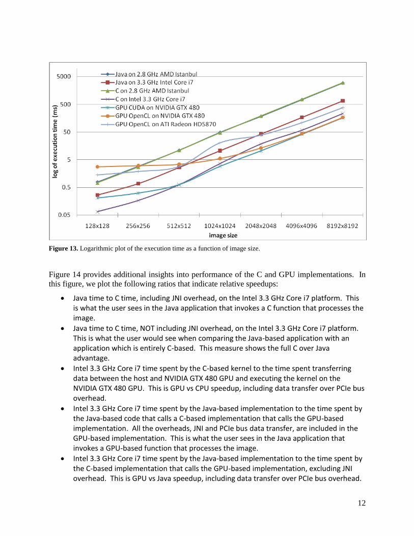
generate the plots shown in Figures 13-15.

Figure 13 provides a plot of the execution time for seven implementation/platform configurations

as a function of image size. In the measurements provided in this plot we included all relevant

overheads, such as JNI overhead and PCIe data transfer overhead. In other words, the measured

execution time is what the user sees in the Java application that invokes one or another type of

kernel (Java, C, or GPU). From this plot, we can make several important observations:

Both Java and C implementations perform substantially worse on the 2.8 GHz AMD Istanbul platform compared to the 3.3 GHz Intel Core i7 platform. It is most likely due to the Java and GCC compiler ports that do not fully take into account all AMD processor’s architecture features.

11

On the 3.3 GHz Intel Core i7 platform, the code in which Java-based computation is replaced with a call to a C-based computation executes faster with a near-constant speedup for all image sizes tested in this study.

For a sufficiently large image size, all GPU-based implementations outperform the CPU-based implementations.

CUDA implementation executed on NVIDIA GTX 480 GPU platform outperforms OpenCL implementations running on both platforms.

Image Size AMD CPU host run time (ms) Intel CPU host run time (ms)

java-based

C-based java-based

C-based

C loop JNI overhead total C loop JNI overhead total

128x128 0.79 0.68 0.05 0.73 0.26 0.03 0.04 0.07

256x256 2.93 2.57 0.16 2.73 0.68 0.10 0.07 0.17

512x512 11.13 10.50 0.44 10.94 2.63 0.42 0.20 0.62

1024x1024 49.22 42.79 4.20 46.99 10.58 1.71 1.91 3.62

2048x2048 185.42 172.91 18.11 191.02 42.23 7.49 11.08 18.57

4096x4096 741.33 692.66 65.91 758.57 168.66 27.54 30.58 58.12

8192x8192 2969.32 2760.50 264.07 3024.56 672.13 110.59 121.85 232.44

Image Size NVIDIA GTX 480 GPU run time (ms)

CUDA-based OpenCL-based

GPU kernel

PCIe overhead

JNI overhead

total GPU kernel

PCIe overhead

JNI overhead

total

128x128 0.05 0.04 0.12 0.21 0.12 0.23 2.45 2.80

256x256 0.06 0.08 0.17 0.31 0.13 0.29 2.65 3.06

512x512 0.08 0.26 0.29 0.63 0.14 0.48 2.82 3.44

1024x1024 0.17 0.73 2.01 2.91 0.24 0.96 4.36 5.56

2048x2048 0.53 2.32 7.71 10.56 0.64 2.59 10.17 13.40

4096x4096 1.96 8.76 30.90 41.62 2.13 8.99 32.91 44.03

8192x8192 7.77 34.49 123.24 165.50 8.20 37.60 124.53 170.33

Image Size ATI Radeon 5870 GPU run time (ms)

OpenCL-based

GPU kernel

PCIe overhead

JNI overhead

total

128x128 0.36 0.44 0.62 1.42

256x256 0.36 0.61 0.92 1.89

512x512 0.41 1.34 1.11 2.86

1024x1024 0.35 15.24 4.90 20.49

2048x2048 0.76 20.39 17.30 38.45

4096x4096 2.53 39.38 67.00 108.91

8192x8192 6.83 108.41 263.60 378.84

Table 3. Performance measurements for different implementations and architectures.

12

Figure 13. Logarithmic plot of the execution time as a function of image size.

Figure 14 provides additional insights into performance of the C and GPU implementations. In

this figure, we plot the following ratios that indicate relative speedups:

Java time to C time, including JNI overhead, on the Intel 3.3 GHz Core i7 platform. This is what the user sees in the Java application that invokes a C function that processes the image.

Java time to C time, NOT including JNI overhead, on the Intel 3.3 GHz Core i7 platform. This is what the user would see when comparing the Java-based application with an application which is entirely C-based. This measure shows the full C over Java advantage.

Intel 3.3 GHz Core i7 time spent by the C-based kernel to the time spent transferring data between the host and NVIDIA GTX 480 GPU and executing the kernel on the NVIDIA GTX 480 GPU. This is GPU vs CPU speedup, including data transfer over PCIe bus overhead.

Intel 3.3 GHz Core i7 time spent by the Java-based implementation to the time spent by the Java-based code that calls a C-based implementation that calls the GPU-based implementation. All the overheads, JNI and PCIe bus data transfer, are included in the GPU-based implementation. This is what the user sees in the Java application that invokes a GPU-based function that processes the image.

Intel 3.3 GHz Core i7 time spent by the Java-based implementation to the time spent by the C-based implementation that calls the GPU-based implementation, excluding JNI overhead. This is GPU vs Java speedup, including data transfer over PCIe bus overhead.

13

From this plot, we can make the following observations:

Replacing optimized Java code with the call to a C-based function results in on average 3x speedup. This speedup takes into account the overhead of calling a C function from the Java application.

We observe an average 6x speedup when comparing Java computation time with the corresponding C-based code computation time, assuming that there is a full C-based application. The speedup is even greater, up to 8.8x, for smaller images. This observation indicates that if the image analysis algorithm used in doc2learn was implemented as a stand-alone C program, it would have executed 6 times faster than the current doc2learn all-Java implementation.

For small images, GPU implementation is actually slower than the C-based CPU implementation. For image sizes close to 512x512, the CPU and GPU implementations break even. Maximum GPU speedup for sufficiently large images is only 2.6x as compared to the C-based CPU implementation.

Replacing optimized Java code with the call to a C function that calls a GPU function results in the speedup ranging from 1.2x for small images to 4x for large images. This is what the user sees from the standpoint of the Java application.

Finally, if we compare full Java-based implementation with the C-based implementation that calls a GPU kernel, we observe a speedup of almost 3x for small images to almost 16x for large images. This observation indicates that if the image analysis algorithm used in doc2learn was implemented as a stand-alone C program that uses NVIDIA GTX 480 GPU, it would have executed up to 16 times faster than the current doc2learn all-Java implementation.

Figure 14. Speedup as a function of image size.

14

Figure 15 provides some additional insights into the image analysis code execution profile for

two image sizes and three platforms. For a sufficiently large image, GPU-based implementation

suffers from a substantial JNI Java-to-C interface overhead.

Java Java+C Java+C+GPU

GPU compute 0.00 0.00 0.53

PCIe overhead 0.00 0.00 2.32

CPU compute 0.00 11.08 0.00

JNI overhead 0.00 7.49 7.71

Java compute 42.23 0.00 0.00

0

5

10

15

20

25

30

35

40

45

exe

cuti

on

tim

e (m

s)

2048x2048 image

Java Java+C Java+C+GPU

GPU compute 0.00 0.00 0.06

PCIe overhead 0.00 0.00 0.08

CPU compute 0.00 0.10 0.00

JNI overhead 0.00 0.07 0.17

Java compute 0.68 0.00 0.00

0.0

0.1

0.2

0.3

0.4

0.5

0.6

0.7

0.8

exe

cuti

on

tim

e (m

s)

256x256 image

Figure 15. Execution profile comparison for two image sizes.

3.6 Performance study to understand the impact of the number of images

We investigate performance of different implementations of the image analysis algorithm as the

function of the number of images embedded in the PDF file. We consider three implementations

using Intel platform:

Java implementation with the optimized Java code running on a single core of 3.3 GHz Intel Core i7 processor

C implementation running on a single core of 3.3 GHz Intel Core i7 processor

CUDA C implementation running on NVIDIA GTX 480 GPU installed on the 3.3 GHz Intel Core i7 platform

The dataset used in this study consists of 100 PDF files that contain only images. Each PDF file

contains some number of randomly generated images of a fixed size. Image sizes include 50x50,

100x100, 150x150, and 200x200 pixels and image count per PDF file is from 10 to 250. This

synthetic dataset was generated by Peter Bajcsy’s team and it is deemed to be statistically

representative of a set of PDF files that the team has been working with.

Table 4 lists all the image sizes and the number of images per PDF file. It also lists the overall

image processing time for each of the PDF files using each of the three algorithm

implementations. Figure 16 provides a graphical representation of the data from Table 4. The

measured execution time confirms our prior findings:

For small images, C-based implementation outperforms both the Java-based and GPU-based implementations

15

JAVA C GPU

Image size Image size Image size

count 50x50 100x100 150x150 200x200 50x50 100x100 150x150 200x200 50x50 100x100 150x150 200x200

10 11 10 13 15 8 9 9 9 12 13 11 11

20 19 20 23 27 18 17 18 20 22 24 22 23

30 28 34 34 40 26 30 27 30 32 32 33 34

40 37 43 45 53 37 37 38 41 43 43 45 46

50 46 50 57 67 44 45 46 51 54 54 56 59

60 56 62 69 79 54 54 56 58 64 66 68 70

70 65 71 80 92 63 65 67 72 75 74 81 82

80 78 82 94 110 72 73 78 80 83 86 87 91

90 87 92 107 124 82 83 87 88 97 99 102 107

100 131 342 135 175 105 283 125 106 120 478 146 120

110 110 125 132 151 104 105 111 114 123 125 129 131

120 118 128 148 168 119 113 120 136 137 136 145 145

130 129 140 156 178 125 127 131 132 146 145 153 156

140 139 149 169 193 130 134 136 141 153 159 159 174

150 146 162 179 205 142 146 151 156 167 172 175 183

160 156 172 189 224 146 154 154 162 180 182 185 194

170 164 184 198 232 159 168 166 173 186 189 193 197

180 180 195 213 253 168 168 170 187 203 202 209 212

190 186 201 224 260 178 182 190 195 218 215 224 219

200 199 212 239 282 188 193 204 201 226 219 229 237

210 199 227 259 289 197 202 201 209 231 238 246 244

220 209 230 260 299 205 205 221 228 237 239 255 260

230 220 237 268 310 216 225 230 239 257 261 265 272

240 228 250 292 327 217 231 233 250 255 265 267 275

250 237 263 290 344 230 231 241 250 271 275 277 287

Table 4. Image processing time (in ms) for different implementations using synthetic dataset consisting of 100 PDF

files with varying number of images (from 10 to 250) per file and different image size (from 50x50 to 200x200

pixels).

16

Figure 16. Execution time as the function of the number of images per PDF file.

4 Conclusions and future work

4.1 Implications for doc2learn image analysis algorithm

The image probability density function computation algorithm implemented in Java in doc2learn

software can be accelerated by a factor of 6x if the entire doc2learn image analysis software is

re-implemented in C, or by a factor of almost 16x if it also uses an NVIDIA GTX 480 GPU.

Actual GPU speedup largely depends on the image size: for images less than 512x512 our CPU

implementation outperforms the GPU implementation.

Calling a GPU-based implementation from the existing doc2learn Java-based code is still

beneficial as it provides up to 4x speedup for sufficiently large images. But another factor of 4x

speedup can be achieved by porting the entire image analysis software suite to C and using GPU

kernels within the C-based code.

4.2 Implications for doc2learn application

Doc2learn execution profile shown in Figure 6 indicates that only about 4% of the overall

execution time for the given PDF file example is spent on the image processing part. Speeding it

up by any factor will not make much of a difference for the entire application. Said that, GPU

acceleration may be still beneficial for PDF files containing very large images or embedded

videos.

Doc2learn also implements probability density function computation algorithms for text and

vector graphics. These data types exhibit less regular memory access patterns and require much

large histograms to be stored. Because of this, they are less suitable for GPU implementation as

compared to image histograms.

17

4.3 CUDA vs OpenCL

At this point, CUDA-based implementation outperforms the OpenCL based implementation, but

it does not provide portability across GPU platforms. We have not investigated OpenCL

implementation for a multi-core architecture, but from our prior experience we know that

platform-specific tuning will be required to achieve good performance with OpenCL on any

architecture. The OpenCL code written for one architecture will execute on another architecture,

but not at its full potential.

4.4 Future work

In the second quarter of this project, we will develop a stand-alone C implementation of the

image extraction component of doc2learn and will integrate the developed image probability

density function computation algorithm (both the CPU and GPU implementations) with the

stand-alone image extractor. We will base our work on xpdf C++ library which has all the

components necessary to quickly assemble the PDF image extraction framework. We will

investigate how to extend the CPU implementation of the histogram computation to the multi-

core architecture of modern CPUs. We will conduct a study how the proposed stand-alone

implementation compares to the original doc2learn implementation, with regards to both the

image processing time and the object extraction time, which is significant in current doc2learn

implementation. We will use the developed stand-alone framework to analyze power

consumption of the CPU and GPU implementations on a set of benchmark PDF files.

We will investigate other image comparison algorithms and their suitability for GPU

acceleration. Versus project currently under development by Peter Bajcsy’s team provides a

framework for using third-party image characterization algorithms. We will investigate pros and

cons of extending this framework to include GPU-based image comparison algorithms.