Evaluation and Calibration of Pedestrian Bridge Standards ...

Evaluation and Calibration ofPedestrian Bridge Standards for

Vibration Serviceability

by

Pampa Dey

A thesispresented to the University of Waterloo

in fulfillment of thethesis requirement for the degree of

Doctor of Philospphyin

Civil Engineering

Waterloo, Ontario, Canada, 2017

c© Pampa Dey 2017

Examining Committee Membership

The following served on the Examining Committee for this thesis. The decision of theExamining Committee is by majority vote.

External Examiner: Mustafa GulAssociate professor,Dept. of Civil and Environmental Engg., University of Alberta

Supervisor(s): Sriram NarasimhanAssociate professor,Dept. of Civil and Environmental Engg., University of WaterlooScott WalbridgeAssociate professor,Dept. of Civil and Environmental Engg., University of Waterloo

Internal Member: Giovanni CascanteProfessor,Dept. of Civil and Environmental Engg., University of WaterlooMahesh PandeyProfessor,Dept. of Civil and Environmental Engg., University of Waterloo

Internal-External Member: Stephen D. PrenticeAssociate professor,Dept. of Kinesiology, University of Waterloo

ii

I hereby declare that I am the sole author of this thesis. This is a true copy of the thesis,including any required final revisions, as accepted by my examiners.

I understand that my thesis may be made electronically available to the public.

iii

Abstract

An increase in the use of lightweight materials and emphasis on architecturally appeal-ing designs has resulted in lively pedestrian bridges. A prominent example for this is theserviceability failure of the London Millenium Bridge in 2001, where excessive vibrationsfrom inauguration crowds resulted in shutting down the structure. While the bridge wassubsequently retrofitted with damping devices, this incident brought often overlooked andpoorly understood issues on pedestrian bridges to the fore. Various load models and designprocedures have since been proposed to assess the serviceability of pedestrian bridges underwalking-induced loads, load modelling being the one that has attracted the most attentionin the recent years. In general, all of the existing design provisions employ a Fourier seriesapproach to modelling the foot-fall force due to a single pedestrian and extrapolate thisto groups through multiplication factors. Despite two decades of use, there are significantdiscrepancies amongst the provisions and little has been done in terms of evaluating them,especially using experimental data.

The main objectives of this thesis are two-fold: first, a comprehensive evaluation ofexisting standards is undertaken to understand the performance of the existing design pro-visions in predicting the actual performance of lively pedestrian bridges; next, changesare recommended based on such experiments to key factors used in the provisions to bet-ter align the observations with the predictions. In the current study, design provisionscurrently being used in North America and Europe are evaluated, including ISO 10137,Eurocode 5, the British National Annex to Eurocode 1, and SETRA. The experimentalprogram was undertaken on three full-scale aluminum pedestrian bridges; one in the fieldand two in the laboratory. Aluminum structures provide a high strength-to-weight ratio,are corrosion resistant, and aesthetically pleasing. Due to their relative light weight, theycan be built in a laboratory environment to full-scale and still produce lively structuresthat can be excited with relatively lower actuation compared to comparable steel or con-crete structures. The current experimental study focuses on such cases where there is thepossibility of resonance with the higher harmonics of the walking frequency, not just thefundamental frequency. The test bridges were instrumented and subjected to a range ofmodal and pedestrian walking tests of varying traffic sizes. The comparison results betweenthe predicted and measured responses show that commonly employed load models for singlepedestrian walking can sometimes be un-conservative. Moreover, the outcomes from theserviceability assessment under crowd-induced loading show significant differences in thepredicted responses by the guidelines with respect to the measurements, which are mainlyattributable to differences in the dynamic load factors adopted in the guidelines, and lackof guidance on the appropriate walking speeds in crowd loading conditions and the factor

iv

scaling the individual pedestrian load to multiple pedestrians. Additionally, the guidelinesare evaluated in a reliability-based framework to incorporate the potential uncertaintiesassociated with the walking loads, structural properties, and occupant comfort limits. Thekey results point towards calibrating the current design provisions to a higher reliabilityindex for the design events in order to achieve sufficiency during the non-frequent or rareloading events.

Hence, an attempt is made towards to improving the predictions by the guidelines.Several recommendations are proposed to harmonize the design provisions with each otherand with measurements. The recommended modifications lead to a substantial improve-ment in the predicted responses by the guidelines. In the next step, the design provisionsare calibrated for higher reliability to achieve acceptable performance during the design aswell as non-frequent (rare) heavy traffic loading events. For this purpose, the reliabilitylevel required for the calibration process is estimated and corresponding partial factors forthe calibrated design are reported. The study also suggests adopting comfort limits basedon the frequency of occurrence of the traffic event and the pedestrian bridge class in orderto yield economic designs.

v

Acknowledgements

I would like to take this opportunity to express my sincere gratitude to all those whohave provided me with guidance and support in various ways through my journey as aDoctoral student.

First and foremost, I would like to express my deepest gratitude to my advisors, Dr.Sriram Narasimhan and Dr. Scott Walbridge for giving me the chance to pursue myDoctoral studies. Both have been great mentors and instilled confidence in me throughoutmy PhD candidature by providing the perfect balance of independence and guidance in myresearch. I am grateful to Dr. Mustafa Gul, Dr. Stephen Prentice, Dr. Giovanni Cascante,Dr. Mahesh Pandey, and Dr. Dipanjan Basu for serving as my committee members andtheir time in reviewing my work.

I want to thank Dr. Stephen Prentice for allowing me to use their Biomechanics lab-oratory to perform walking force measurements. I have also been fortunate to have Dr.Arndt Goldack from TU Berlin visiting University of Waterloo during the course of theexperimental studies. His insights during the experimental work have played a significantrole in improving some aspects of the laboratory bridge specimen.

I would also like to take this opportunity to acknowledge the Most Advanced AluminiumDesign and Inspection (MAADI) Group and the Aluminium Association of Canada for sup-porting us with the experimental set-up, including the full scale Make-A-Bridge aluminiumpedestrian bridge lab specimen.

I would like to say a big Thank You to Ann Sychterz for her collaboration on theexperimental studies. I want to extend my sincere gratitude to the technicians of theStructures laboratory, Richard Morrison, Michael Burgetz and Rob Sluban, for their helpand support in building the bridges and designing instrumentation, which has been verymonumental for my thesis. I am also thankful to all the volunteers and undergraduateresearch assistants who were part of the walking tests on the laboratory bridge specimens,with my special acknowledgment to Kevin, Rajdip, Rakesh, Guru, Roya, Stan, Shilpa,Ben, Amr, Laura, and Melissa.

Any attempt to thank my parents, sisters and brother-in-law: Baba, Ma, Didi, Jiju, andMithu, would fall short. Their love, support, and encouragement have been my primarymotivation. Last but not least, I owe my deepest gratitude to my dear husband Satya forbeing by my side throughout the roller coaster journey. Your unconditional love and trusthas always been a source of support and encouragement to continue my passion.

vi

Dedication

To Baba, Ma, Didi, Jiju, Mithu, and Satya

vii

Table of Contents

List of Tables xi

List of Figures xiii

1 Introduction 1

1.1 General Introduction . . . . . . . . . . . . . . . . . . . . . . . . . . . . . . 1

1.2 Objectives of the research . . . . . . . . . . . . . . . . . . . . . . . . . . . 3

1.3 Organization of the thesis . . . . . . . . . . . . . . . . . . . . . . . . . . . 3

2 Background 5

2.1 Pedestrian-induced walking loads . . . . . . . . . . . . . . . . . . . . . . . 5

2.1.1 Basics of walking . . . . . . . . . . . . . . . . . . . . . . . . . . . . 5

2.1.2 Walking force measurements . . . . . . . . . . . . . . . . . . . . . . 8

2.1.3 Walking load models . . . . . . . . . . . . . . . . . . . . . . . . . . 9

2.1.4 Limitations of existing walking load models . . . . . . . . . . . . . 20

2.2 Vibration serviceability design of PBs . . . . . . . . . . . . . . . . . . . . . 21

2.2.1 A two-step approach . . . . . . . . . . . . . . . . . . . . . . . . . . 21

2.2.2 Dynamic analysis . . . . . . . . . . . . . . . . . . . . . . . . . . . . 23

2.3 Structural response simulation under walking loads . . . . . . . . . . . . . 32

2.4 Full-scale experiments on PBs . . . . . . . . . . . . . . . . . . . . . . . . . 33

2.5 Gap areas in existing research on vibration serviceability of PBs . . . . . . 35

2.6 Specific objectives . . . . . . . . . . . . . . . . . . . . . . . . . . . . . . . . 37

viii

3 Experimental evaluation of design provisions using tests on full-scalebridges 38

3.1 Experimental program . . . . . . . . . . . . . . . . . . . . . . . . . . . . . 38

3.1.1 Description of the bridges . . . . . . . . . . . . . . . . . . . . . . . 39

3.1.2 Instrumentation . . . . . . . . . . . . . . . . . . . . . . . . . . . . . 39

3.1.3 Testing program . . . . . . . . . . . . . . . . . . . . . . . . . . . . 41

3.1.4 Dynamic properties of the bridges . . . . . . . . . . . . . . . . . . . 43

3.2 Performance of design guidelines . . . . . . . . . . . . . . . . . . . . . . . . 45

3.2.1 Single pedestrian load model . . . . . . . . . . . . . . . . . . . . . . 47

3.2.2 Serviceability assessment under groups of pedestrians . . . . . . . . 61

4 Reliability-based evaluation of design provisions 74

4.1 Sources of uncertainty . . . . . . . . . . . . . . . . . . . . . . . . . . . . . 74

4.1.1 Uncertainties in the pedestrian load . . . . . . . . . . . . . . . . . . 75

4.1.2 Uncertainties in the limit acceleration . . . . . . . . . . . . . . . . . 77

4.1.3 Uncertainties in the structural properties . . . . . . . . . . . . . . . 77

4.2 Range of design variables . . . . . . . . . . . . . . . . . . . . . . . . . . . . 79

4.2.1 Structural configurations . . . . . . . . . . . . . . . . . . . . . . . . 79

4.2.2 Design traffic . . . . . . . . . . . . . . . . . . . . . . . . . . . . . . 79

4.3 Calculation of reliability index . . . . . . . . . . . . . . . . . . . . . . . . . 81

4.4 Reliability analysis . . . . . . . . . . . . . . . . . . . . . . . . . . . . . . . 85

4.4.1 Reliability-based design criteria . . . . . . . . . . . . . . . . . . . . 85

4.4.2 Results from reliability analysis . . . . . . . . . . . . . . . . . . . . 86

4.4.3 Parametric study . . . . . . . . . . . . . . . . . . . . . . . . . . . . 94

4.4.4 Summary of key results from the reliability analysis . . . . . . . . . 103

ix

5 Recommendations to improve existing design provisions and reliability-based code calibration 104

5.1 Recommendations for serviceability design . . . . . . . . . . . . . . . . . . 104

5.1.1 Key design recommendations . . . . . . . . . . . . . . . . . . . . . 105

5.1.2 Effect of the recommended changes . . . . . . . . . . . . . . . . . . 107

5.1.3 Reliability analysis after the proposed modifications . . . . . . . . . 108

5.2 Reliability-based calibration . . . . . . . . . . . . . . . . . . . . . . . . . . 109

5.2.1 Calibration process . . . . . . . . . . . . . . . . . . . . . . . . . . . 111

5.2.2 Results of calibration . . . . . . . . . . . . . . . . . . . . . . . . . . 115

6 Conclusions and recommendations 134

6.1 Significant contributions . . . . . . . . . . . . . . . . . . . . . . . . . . . . 134

6.2 Conclusions . . . . . . . . . . . . . . . . . . . . . . . . . . . . . . . . . . . 135

6.3 Limitations of the current study . . . . . . . . . . . . . . . . . . . . . . . . 138

6.4 Recommendations for future study . . . . . . . . . . . . . . . . . . . . . . 138

References 140

APPENDICES 149

A Response simulation 150

B Mode shapes from finite element models 153

C Modal identification through free vibration tests 156

C.1 Fast Fourier Transform or FFT method . . . . . . . . . . . . . . . . . . . . 156

C.2 Modal damping estimation . . . . . . . . . . . . . . . . . . . . . . . . . . . 157

D TLS-Prony’s method 159

x

List of Tables

2.1 Summary of proposed DLF values reported in the literature . . . . . . . . 13

2.2 Statistics os step frequency by different researchers . . . . . . . . . . . . . 14

2.3 Limiting frequencies proposed by different design guidelines . . . . . . . . . 22

2.4 Acceleration limits specified in guidelines . . . . . . . . . . . . . . . . . . . 23

2.5 Design parameters for moving forces due to one person according to ISO10137.2007 . . . . . . . . . . . . . . . . . . . . . . . . . . . . . . . . . . . . 25

2.6 Frequency ranges for vertical and lateral vibrations . . . . . . . . . . . . . 30

2.7 Load cases considered for different fundamental frequency ranges . . . . . . 30

3.1 Physical and gait parameters of test subjects in the Daigneault Creek Bridgestudy . . . . . . . . . . . . . . . . . . . . . . . . . . . . . . . . . . . . . . . 43

3.2 Physical and gait parameters of test subjects in the 12.2 m bridge study . 43

3.3 Physical and gait parameters of test subjects in the 22.9 m bridge study . 44

3.4 Test matrix for 12.2 m pedestrian bridge . . . . . . . . . . . . . . . . . . . 44

3.5 Test matrix for 22.9 m pedestrian bridge . . . . . . . . . . . . . . . . . . . 45

3.6 Natural frequencies and mode shapes for the bridges through finite elementanalysis and modal testing . . . . . . . . . . . . . . . . . . . . . . . . . . . 45

3.7 Damping ratio for the bridges through modal testing . . . . . . . . . . . . 45

3.8 Multiplication factors for crowd loading used by existing guidelines . . . . 47

3.9 Dynamic load factors adopted by guidelines and standards . . . . . . . . . 48

3.10 Mean and standard deviation for the experimental peak accelerations on the12.2. and 22.9 m bridge specimens . . . . . . . . . . . . . . . . . . . . . . 65

xi

4.1 Statistical properties of elastic modulus for different structural material . . 78

4.2 Average damping ratios for steel/aluminum . . . . . . . . . . . . . . . . . 79

4.3 Traffic classes in various guidelines . . . . . . . . . . . . . . . . . . . . . . 80

4.4 PB classes and corresponding traffic sizes for the reliability analysis . . . . 81

4.5 Ranges of reliability index (βrange = βmax − βmin) for different PB classes . 90

4.6 Summary of reliability results for different PB classes . . . . . . . . . . . . 93

5.1 Summary of cases based on comfort limits for pedestrians . . . . . . . . . . 111

5.2 Partial factors corresponding to different target reliability index . . . . . . 116

5.3 Desired reliability by different guidelines for different cases . . . . . . . . . 117

5.4 Desired reliability and reliability implied (in brackets) by different guidelinesfor Class I of PBs in case of R15 for different COVs of al . . . . . . . . . . 121

xii

List of Figures

2.1 Schematic diagram of a complete gait cycle during normal walking (repro-duced from Simoneau (2002)) . . . . . . . . . . . . . . . . . . . . . . . . . 6

2.2 (a) GRF of a single step in the vertical direction; (b) GRF for continuouswalking in the vertical direction; (c) Fourier spectrum of the GRF in thevertical direction; (d) GRF of a single step in the lateral direction; (e) GRFfor continuous walking in the lateral direction, and (f) Fourier spectrum ofthe GRF in the lateral direction, by a person walking at 2 Hz . . . . . . . 7

2.3 Dynamic load factors (DLFs) for first four harmonics of walking (taken fromRainer et al. (1988)) . . . . . . . . . . . . . . . . . . . . . . . . . . . . . . 11

2.4 Dynamic load factors (DLFs) reported in the literature (taken from Willfordet al. (2006)) . . . . . . . . . . . . . . . . . . . . . . . . . . . . . . . . . . 12

2.5 Distribution of step frequency for normal walking . . . . . . . . . . . . . . 15

2.6 Distribution of walking speeds at 1.8 Hz (reproduced from Zivanovic (2006)) 16

2.7 (a)Two degree of freedom SMD model as adopted by Kim et al. (2008),(b) inverted pendulum model as adopted by Bocian et al. (2012) and (c)bipedal-walking model as adopted by Qin et al. (2013) . . . . . . . . . . . 18

2.8 Base curves in accordance to ISO 10137 for (a) vertical and (b) lateraldirections . . . . . . . . . . . . . . . . . . . . . . . . . . . . . . . . . . . . 24

2.9 (a) Vertical and (b) lateral response reduction factors in accordance withEurocode 5 . . . . . . . . . . . . . . . . . . . . . . . . . . . . . . . . . . . 27

2.10 (a) Vertical response reduction factor, (b) reduction factor γ as a functionof the logarithmic decrement, and (c) the damping factor as a function ofthe lateral mode by the British National Annex . . . . . . . . . . . . . . . 28

xiii

2.11 Response reduction factor (ψ) in the (a) vertical and (b) lateral directionsaccordance with SETRA guideline . . . . . . . . . . . . . . . . . . . . . . . 31

2.12 Moving load on a simply supported PB . . . . . . . . . . . . . . . . . . . . 33

3.1 (a) Daigneault Creek Bridge of span 43.7 m, (b) Modular aluminum bridgeof span 22.9 m, and (c) Modular aluminum bridge of span 12.2 m . . . . . 40

3.2 Basic assembly of Make-A-Bridge R© specimen . . . . . . . . . . . . . . . . 41

3.3 (a)Plan view of the bridge of length 22.9 m with locations for the instru-mentation showing (b) accelerometers, (c) vibration data collection system(d) load cells, (e) displacement transducer . . . . . . . . . . . . . . . . . . 42

3.4 (a) One pedestrian and (b) groups of pedestrians walking on the 22.9 mbridge specimen during the experimental study carried out in the StructuresLaboratory at the University of Waterloo . . . . . . . . . . . . . . . . . . . 46

3.5 Acceleration time history ((a) and (c)) and corresponding Fourier spectrum((b) and (d)) of impact testing at centre ((a) and (b)) and quarter (((c) and(d))) spans of the 22.9 m bridge specimen . . . . . . . . . . . . . . . . . . 46

3.6 The acceleration time history at the centre of the Daigneault Creek Bridgefor walking at 2.0 Hz in the case of simulated response using (a) ISO 10137,(b) Eurocode 5, (c) British National Annex, and (d) SETRA models and(e) field measurements (Here, M are R represents respectively the maximumand RMS accelerations) . . . . . . . . . . . . . . . . . . . . . . . . . . . . 51

3.7 Fourier spectra of the acceleration response at the centre of the DaigneaultCreek Bridge for walking at 2.0 Hz in the case of simulated response using(a) ISO 10137, (b) Eurocode 5, (c) British National Annex, and (d) SETRAmodels and (e) field measurements . . . . . . . . . . . . . . . . . . . . . . 52

3.8 The acceleration time history at the centre of the Daigneault Creek Bridgefor walking at 1.75 Hz in the case of simulated response using (a) ISO 10137,(b) Eurocode 5, (c) British National Annex, and (d) SETRA models and(e) field measurements (Here, M are R represents respectively the maximumand RMS accelerations) . . . . . . . . . . . . . . . . . . . . . . . . . . . . 53

3.9 Fourier spectra of the acceleration response at the centre of the DaigneaultCreek Bridge for walking at 1.75 Hz in the case of simulated response using(a) ISO 10137, (b) Eurocode 5, (c) British National Annex, and (d) SETRAmodels and (e) field measurements . . . . . . . . . . . . . . . . . . . . . . 54

xiv

3.10 Comparison of simulated and measured amplitudes corresponding to: (a) thefirst harmonic, (b) the second harmonic, and (c) the fundamental frequency,in the case of Daigneault Creek Bridge . . . . . . . . . . . . . . . . . . . . 56

3.11 Statistical results for simulated and measured amplitudes corresponding toP5 for: (a) the first harmonic, (b) the second harmonic, and (c) the naturalfrequencies for the Daigneault Creek Bridge . . . . . . . . . . . . . . . . . 57

3.12 Comparison of contributions for simulated and measured amplitudes fromthe: (a) first harmonic (b) fifth harmonic, (c) sixth harmonic, and (d) nat-ural frequency in the case of the 12.2 m bridge specimen . . . . . . . . . . 58

3.13 Simulated and measured amplitude contributions corresponding to the: (a)first harmonic, (b) second harmonic, (c) third harmonic, and (d) naturalfrequencies for the 22.9 m bridge specimen . . . . . . . . . . . . . . . . . . 60

3.14 Results from the 12.2 m bridge specimen under 1.0 P/m2 crowd density: (a)acceleration time history in the vertical direction at the center, (b) spec-trogram, (c) Fourier spectrum, (d) acceleration time history for the lateraldirection at the center and its corresponding (e) spectrogram, (f) Fourierspectrum. . . . . . . . . . . . . . . . . . . . . . . . . . . . . . . . . . . . . 63

3.15 Results from the 22.9 m bridge specimen under 0.7 P/m2 crowd density: (a)acceleration time history in the vertical direction at the center, (b) spec-trogram, (c) Fourier spectrum, (d) acceleration time history for the lateraldirection at the center and its corresponding (e) spectrogram, (f) Fourierspectrum. . . . . . . . . . . . . . . . . . . . . . . . . . . . . . . . . . . . . 64

3.16 Comparison of measured and predicted peak accelerations along with thecomfort limits as proposed by guidelines in the vertical direction for the (a)12.2 m and (b) 22.9 m bridge (P stands for pedestrians; Limit I, Limit IIand Limit III by SETRA guideline are defined in Table 2.4) . . . . . . . . 66

3.17 Comparison of measured and predicted peak accelerations along with thecomfort limits as proposed by guidelines in the lateral direction for the (a)12.2 m and (b) 22.9 m bridge (P stands for pedestrians; Limit I, Limit IIand Limit III by SETRA guideline are defined in Table 2.4) . . . . . . . . 67

4.1 Probability density function (PDF) of: (a) pedestrian’s weight (G); (b) DLF(αm); (c) damping ratio (ζ); (d) limit acceleration (al), and (e) elastic mod-ulus (E) . . . . . . . . . . . . . . . . . . . . . . . . . . . . . . . . . . . . . 76

xv

4.2 Mean of reliability indices estimated for all the designs satisfying ψs = 1.0−1.1, using three reliability methods for different classes: (a) ISO 10137, (b)Eurocode 5, (c) British National Annex (group), (d) British National Annex(crowd), and (e) SETRA . . . . . . . . . . . . . . . . . . . . . . . . . . . . 87

4.3 Reliability index as a function of structural frequency for Class II bridgesunder a design traffic of 0.5 P/m2: (a) ISO 10137, (b) Eurocode 5, (c) BritishNational Annex (group), (d) British National Annex (crowd), and (e) SETRA. 88

4.4 Reliability index as a function of structural frequency for Class IV bridgesunder a design traffic of 1.0 P/m2: (a) ISO 10137, (b) Eurocode 5, (c) BritishNational Annex (group), (d) British National Annex (crowd), and (e) SETRA. 89

4.5 Maximum and minimum reliability levels for designs satisfying ψs = 1.0−1.1for different classes: (a) ISO 10137, (b) Eurocode 5, (c) British NationalAnnex (group), (d) British National Annex (crowd), and (e) SETRA . . . 91

4.6 Minimum reliability levels (βmin calculated for the PBs (φs = 1.0−1.1) underdifferent design cases: (a) ISO 10137, (b) Eurocode 5, (c) British NationalAnnex (group), (d) British National Annex (crowd), and (e) SETRA (redmarkers correspond to the design traffic of the particular PB class) . . . . 92

4.7 Variation of mean reliability index with coefficients of variation for al fordifferent PB classes: (a) ISO 10137, (b) Eurocode 5, (c) British NationalAnnex (group), (d) British National Annex (crowd), and (e) SETRA . . . 96

4.8 Variation of mean reliability index with different distribution of ζ for differ-ent PB classes: (a) ISO 10137, (b) Eurocode 5, (c) British National Annex(group), (d) British National Annex (crowd), and (e) SETRA . . . . . . . 97

4.9 Mean of reliability indices estimated for all the optimal designs with andwithout considering uncertainties in E, I and m for different PB classes: (a)ISO 10137, (b) Eurocode 5, (c) British National Annex (group), (d) BritishNational Annex (crowd), and (e) SETRA . . . . . . . . . . . . . . . . . . . 98

4.10 Reliability index values estimated with and without considering uncertain-ties in E, I and m for all the code-designed PBs of class II under designtraffic of 0.5 P/m2: (a) ISO 10137, (b) Eurocode 5, (c) British NationalAnnex (group), (d) British National Annex (crowd), and (e) SETRA. . . . 99

4.11 Variation of mean reliability index with coefficients of variation of ζ fordifferent PB classes: (a) ISO 10137, (b) Eurocode 5, (c) British NationalAnnex (group), (d) British National Annex (crowd), and (e) SETRA . . . 100

xvi

4.12 Variation of mean reliability index with different distribution of ζ for differ-ent PB classes: (a) ISO 10137, (b) Eurocode 5, (c) British National Annex(group), (d) British National Annex (crowd), and (e) SETRA . . . . . . . 101

4.13 Mean of reliability indices estimated for all the optimal designs with andwithout considering uncertainties in structural variables for different PBclasses: (a) ISO 10137, (b) Eurocode 5, (c) British National Annex (group),(d) British National Annex (crowd), and (e) SETRA . . . . . . . . . . . . 102

5.1 Comparison of measurements and peak accelerations predicted by the recom-mended methodology with comfort limits as proposed by several guidelinesin the vertical ((a) and (b)) and the lateral directions ((c) and (d)) for the12.2 m ((a) and (c)) and 22.9 m ((b) and (d)) bridge specimens (P stands forpedestrians; Limit I, Limit II and Limit III by SETRA guideline are definedin Table 2.4) . . . . . . . . . . . . . . . . . . . . . . . . . . . . . . . . . . . 122

5.2 Maximum and minimum reliability levels for different footbridge classes de-signed with and without θe: (a) ISO 10137, (b) Eurocode 5, (c) BritishNational Annex (group), (d) British National Annex (crowd), and (e) SETRA123

5.3 Reliability index for the optimally designed PBs of Class IV with and with-out considering θe: (a) ISO 10137, (b) Eurocode 5, (c) British NationalAnnex (group), (d) British National Annex (crowd), and (e) SETRA . . . 124

5.4 Variation in the mean reliability index with different levels of uncertainty(COV) in the model error term (θe) for various classes of PBs: (a) ISO 10137,(b) Eurocode 5, (c) British National Annex (group), (d) British NationalAnnex (crowd), and (e) SETRA (D stands for deterministic θe) . . . . . . 125

5.5 Desired reliability by different guidelines for different cases of comfort limits 126

5.6 Mean reliability levels implied in ISO 10137 for different PB classes: (a)before calibration (without θen), (b) after calibration (without θen) and (c)after calibration (with θen) . . . . . . . . . . . . . . . . . . . . . . . . . . . 127

5.7 Mean reliability levels implied in Eurocode 5 for different PB classes: (a)before calibration (without θen), (b) after calibration (without θen) and (c)after calibration (with θen) . . . . . . . . . . . . . . . . . . . . . . . . . . . 128

5.8 Mean reliability levels implied in British National Annex to Eurocode 1(group) for different PB classes: (a) before calibration (without θen), (b)after calibration (without θen) and (c) after calibration (with θen) . . . . . 129

xvii

5.9 Mean reliability levels implied in British National Annex to Eurocode 1(crowd) for different PB classes: (a) before calibration (without θen), (b)after calibration (without θen) and (c) after calibration (with θen) . . . . . 130

5.10 Mean reliability levels implied in SETRA for different PB classes: (a) beforecalibration (without θen), (b) after calibration (without θen) and (c) aftercalibration (with θen) . . . . . . . . . . . . . . . . . . . . . . . . . . . . . . 131

5.11 Variation in partial factors with COV of limit acceleration for different targetreliability levels (βt) corresponding to (a) al (m=1), (b) al (m > 1), (c) G(m = 1), (d) G (m > 1), (e) αm (m = 1) and (f) αm (m > 1), where m isthe resonating harmonic of walking frequency . . . . . . . . . . . . . . . . 132

5.12 Desired reliability by different guidelines for Class I of PBs in case of R15

for different COVs of al . . . . . . . . . . . . . . . . . . . . . . . . . . . . . 133

B.1 First lateral mode at 2.3 Hz for the 12.2 m bridge specimen . . . . . . . . 153

B.2 First vertical mode at 13.0 Hz for the 12.2 m bridge specimen . . . . . . . 154

B.3 First lateral mode at 1.0 Hz for the 22.9 m bridge specimen . . . . . . . . 154

B.4 First vertical mode at 4.4 Hz for the 22.9 m bridge specimen . . . . . . . . 154

B.5 First vertical mode at 3.40 Hz for the Daigneault Creek bridge specimen(taken from Sychterz et al. (2013)) . . . . . . . . . . . . . . . . . . . . . . 155

C.1 (a) Exponential envelop fitted to first vertical modal acceleration time his-tory and (b) illustration of decaying time history with successive peaks,measured at the mid span of the 22.9 m bridge specimen during hammer test157

xviii

Chapter 1

Introduction

1.1 General Introduction

Structural designs are traditionally governed by their strength or load carrying capacity,which is known as the ultimate limit state design (ULS). However, recent design trendstowards high-strength and light-weight construction materials, especially in pedestrianbridges, have made them more susceptible to vibration serviceability problems under walk-ing service loads. Furthermore, compared to ULS failure events, serviceability failures occurmore frequently. While the cost of individual serviceability failure events can be less, thecumulative economic impact of serviceability failures can be significant. Previous surveyshave shown that considerable costs can be incurred due to serviceability failures, ratherthan strength, and thus serviceability issues cannot be underestimated (Stewart, 1996).Therefore, vibration serviceability has become a dominant criterion in structural designover the last two decades (Allen and Murray, 1993; Willford et al., 2006) and has sincebeen increasingly the focus of researchers worldwide.

Issues related to vibration serviceability of structures under human activities have beenidentified since the 19th century (Tredgold, 1890). However, the possibility of resonance hasbeen ignored in their design until recently. Pedestrian bridges (PBs) are prone to vibrationsdue to one or more natural frequencies falling within the range of typical human activitiessuch as walking, running, bouncing or jumping. Among all these activities, walking is themost frequently occurring one and thus is the primary source of excitation in PBs. Someof the well publicized incidents of serviceability failures of PBs under walking-inducedexcitations include the London Millennium bridge (Dallard et al., 2001), the Pont duSolferino in Paris (Danbon and Grillaud, 2005) and the T-Bridge in Japan (Fujino et al.,

1

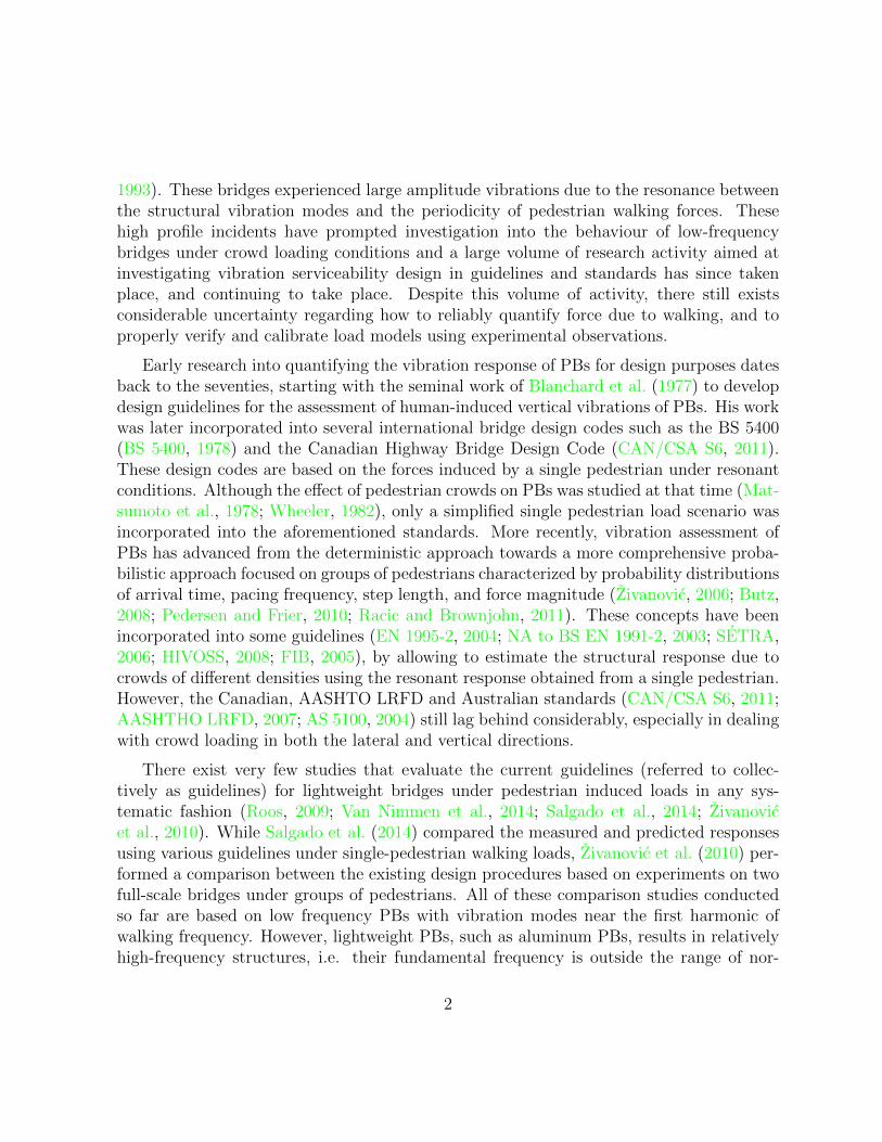
1993). These bridges experienced large amplitude vibrations due to the resonance betweenthe structural vibration modes and the periodicity of pedestrian walking forces. Thesehigh profile incidents have prompted investigation into the behaviour of low-frequencybridges under crowd loading conditions and a large volume of research activity aimed atinvestigating vibration serviceability design in guidelines and standards has since takenplace, and continuing to take place. Despite this volume of activity, there still existsconsiderable uncertainty regarding how to reliably quantify force due to walking, and toproperly verify and calibrate load models using experimental observations.

Early research into quantifying the vibration response of PBs for design purposes datesback to the seventies, starting with the seminal work of Blanchard et al. (1977) to developdesign guidelines for the assessment of human-induced vertical vibrations of PBs. His workwas later incorporated into several international bridge design codes such as the BS 5400(BS 5400, 1978) and the Canadian Highway Bridge Design Code (CAN/CSA S6, 2011).These design codes are based on the forces induced by a single pedestrian under resonantconditions. Although the effect of pedestrian crowds on PBs was studied at that time (Mat-sumoto et al., 1978; Wheeler, 1982), only a simplified single pedestrian load scenario wasincorporated into the aforementioned standards. More recently, vibration assessment ofPBs has advanced from the deterministic approach towards a more comprehensive proba-bilistic approach focused on groups of pedestrians characterized by probability distributionsof arrival time, pacing frequency, step length, and force magnitude (Zivanovic, 2006; Butz,2008; Pedersen and Frier, 2010; Racic and Brownjohn, 2011). These concepts have beenincorporated into some guidelines (EN 1995-2, 2004; NA to BS EN 1991-2, 2003; SETRA,2006; HIVOSS, 2008; FIB, 2005), by allowing to estimate the structural response due tocrowds of different densities using the resonant response obtained from a single pedestrian.However, the Canadian, AASHTO LRFD and Australian standards (CAN/CSA S6, 2011;AASHTHO LRFD, 2007; AS 5100, 2004) still lag behind considerably, especially in dealingwith crowd loading in both the lateral and vertical directions.

There exist very few studies that evaluate the current guidelines (referred to collec-tively as guidelines) for lightweight bridges under pedestrian induced loads in any sys-tematic fashion (Roos, 2009; Van Nimmen et al., 2014; Salgado et al., 2014; Zivanovicet al., 2010). While Salgado et al. (2014) compared the measured and predicted responsesusing various guidelines under single-pedestrian walking loads, Zivanovic et al. (2010) per-formed a comparison between the existing design procedures based on experiments on twofull-scale bridges under groups of pedestrians. All of these comparison studies conductedso far are based on low frequency PBs with vibration modes near the first harmonic ofwalking frequency. However, lightweight PBs, such as aluminum PBs, results in relativelyhigh-frequency structures, i.e. their fundamental frequency is outside the range of nor-

2

mal walking frequency. Hence, they have thus far not attracted much attention in theliterature. However, their relative light weight and low intrinsic damping often results inresonance with the higher harmonics of walking frequency and not with the first harmonic,which could lead to significant serviceability issues. Evaluation and comparison of designprovisions for such lightweight PBs with the potential risk of resonance with the higherharmonics of walking frequencies, is lacking. On the other hand, none of these guidelineshave been evaluated in a reliability-based framework incorporating uncertainties arisingfrom pedestrian loads, the structure, and comfort limits for the pedestrians. Moreover,despite significant disagreement observed between measurements and predictions by thedesign guidelines in resonance (mostly with the first harmonics of walking frequency), no at-tempts have been made yet to better align observations with predictions by the guidelines,at the same time ensuring reliable and economical designs. Hence, the main motivationfor this work is to evaluate, and subsequently improve the existing vibration serviceabilitydesign guidelines using extensive experimental tests on full-scale pedestrian bridges.

1.2 Objectives of the research

The overarching objectives of the proposed research are summarized as follows:

• Evaluate the most popular design guidelines in both deterministic and reliability-based frameworks in predicting the performance of lively pedestrian bridges un-der walking-induced excitations through experimental study conducted on full-scalepedestrian bridges that resonate with the higher harmonics of walking frequency.

• Improve the vibration serviceability design provisions for PBs, in order to ensuremore reliable and economical designs, at the same time reconciling the inconsistencieswithin the existing guidelines and between the guidelines and the observations.

1.3 Organization of the thesis

The thesis contains 6 chapters and is organized as follows:

• Chapter 1 provides a brief introduction to the problem of vibration serviceabilityevaluation of pedestrian bridges and a summary of research objectives.

3

• A detailed background on the widely used pedestrian load models is presented inChapter 2. First, the conventional deterministic periodic load model is reviewed,followed by the probabilistic and biomechanical load models. Crowd-induced exci-tation and resulting structural response is also discussed. Next, the existing designguidelines for serviceability assessment of PBs are briefly reviewed along with themethodology to estimate the structural response through the design load models.

• Chapter 3 presents the experimental program involving full-scale aluminum PBs,both in the field and laboratory, with a brief description of the structures followed bythe instrumentation used and the test matrix. The performance of the periodic loadmodel in predicting the response of PBs in the vertical direction is assessed throughmeasurements, followed by evaluating the existing design provisions in predicting theserviceability of these pedestrian bridges under crowd-induced excitation.

• Chapter 4 presents an overview of all possible sources of uncertainties in the designequations by the existing guidelines, followed by evaluation of the design provisionsfor sufficient and uniform reliability under all possible traffic conditions in the designlife of the structure.

• Chapter 5 demonstrates key design recommendations proposed in order to recon-cile the design guidelines with measurements. Moreover, the design provisions arecalibrated in order to achieve sufficient reliability under all possible traffic conditionson the bridge.

• Finally, a number of conclusions resulting from the presented work are discussed inChapter 6. Several recommendations for future study are also discussed, followedby a summary of the significant contributions of the current work.

4

Chapter 2

Background

A review of the background on the walking load models is presented first, including thetime-domain periodic load model and current trends using the biomechanics principles ofwalking. Existing design guidelines in the context of serviceability assessment of PBs underwalking-induced excitation are then reviewed, followed by a methodology to predict thebridge responses. Finally, a brief review on the full-scale studies of PBs under pedestrian-induced walking loads is presented.

2.1 Pedestrian-induced walking loads

2.1.1 Basics of walking

According to Whittle (2003), normal human walking is the gait used by humans whenthey walk at low speeds. A complete gait cycle is the time period between two identicalevents during the walking process, and consists of two phases: stance and swing (Perry,1992). Alternatively, a complete gait cycle can also be represented by right and left steps.An illustration for a complete gait cycle is shown in Figure 2.1. The stance phase refersto the period during which the foot is in contact with the ground while the swing phaserefers to the period when the foot is off the ground. The stance phase starts with the heelstriking the ground, known as initial contact, and ends with the toe off the ground. Atthe same time, the human body passes through two stages during the walking process,the double- and the single-support stages. In the double-support stage, both feet are incontact with the ground, while single-support occurs with the contact of only one leg. In

5

general, a walking process is described through temporal and spatial parameters. Whilewalking speed, pacing rate or walking frequency, and the gait cycle time are typically thetemporal parameters, spatial parameters are step length, step width, and stride length.

Figure 2.1: Schematic diagram of a complete gait cycle during normal walking (reproducedfrom Simoneau (2002))

During walking, the acceleration and deceleration movement of body’s centre of mass(COM) generates ground reaction forces (GRF), which transfer to the ground throughcontact of each foot during the stance phase of gait. The principal directions of GRFsare vertical, lateral, and longitudinal. Of these the vertical and lateral are of primaryinterest for the vibration study of PBs. In Figure 2.2, a typical GRF of a person weighing65 kg as projected onto vertical and lateral directions is shown, both for a single step(left and right leg) as well as for continuous walking, alongside their Fourier spectra. TheGRF measurements were collected by the author from force plates at the BiomechanicalLaboratory at the University of Waterloo.

6

0 0.5 1Time (sec)

0

200

400

600

800

GR

F (N

)

Vertical

0 0.5 1Time (sec)

-100

0

100Lateral

0 1 2 3Time (sec)

0

200

400

600

800

GR

F (N

)

Left leg

Right leg

Continuous

0 1 2 3Time (sec)

-100

0

100

0 5 10 15Frequency(Hz)

0

50

100

150

Four

ier

Am

plitu

des

0 5 10 15Frequency(Hz)

0

20

40

(c) (f)

(e)(b)

(d)(a)

2.0

4.0

6.0

1.0

3.0

5.0

Figure 2.2: (a) GRF of a single step in the vertical direction; (b) GRF for continuouswalking in the vertical direction; (c) Fourier spectrum of the GRF in the vertical direction;(d) GRF of a single step in the lateral direction; (e) GRF for continuous walking in thelateral direction, and (f) Fourier spectrum of the GRF in the lateral direction, by a personwalking at 2 Hz

7

2.1.2 Walking force measurements

There have been numerous attempts to measure the GRFs induced by a single pedestrian.Gait cycle tests have been performed on several types of surfaces, including transducer-equipped floor surface or short walkways (Blanchard et al., 1977; Rainer et al., 1988) andinstrumented treadmills (Dierick et al., 2004; Riley et al., 2007). One of the earliest mea-surements of walking forces from a single step was conducted by Elftman (1938) usinga force plate. Following this work, several single-step measurements were carried out byother researchers (Harper, 1962; Galbraith and Barton, 1970; Wheeler, 1982; Kerr, 1998)using force plates. However, as the forces from two steps are not always identical, ex-tending single step force measurements may not be a correct representation of continuouswalking forces. Hence, more advanced measurements of continuous walking forces com-prising several consecutive steps were carried out by several researchers. While Blanchardet al. (1977) designed a ”gait machine” to continuously measure walking forces, Raineret al. (1988) employed a floor strip with known dynamic properties to measure GRFsfrom consecutive steps. Subsequently, several researchers (Ebrahimpour et al., 1994; Gardet al., 2004) utilized short instrumented walkways with multiple force plates to captureforces from several steps. In all these studies, it was observed that the measured timehistories were approximately periodic. However, there are some associated downsides ofusing floor-mounted force plates for measurement of GRFs. Force plate measurements areusually time consuming and require mounting multiple force plates on walkways or floors.Moreover, deliberately targeting the force plates while walking trials can alter the naturalwalking pattern (Perry, 1992).

In order to overcome the shortcomings from force plate measurements, instrumentedtreadmills have been used for quick collection of continuous GRFs over a wide range ofsteady-state gait speeds (Dierick et al., 2004). Recently, Riley et al. (2007) conducted aseries of experiments on an advanced treadmill system and compared the two modes ofmeasurements of walking forces (force plates and treadmill). They concluded that tread-mill gait is qualitatively and quantitatively very similar to that through measurementsfrom force plates or transducer-equipped surfaces. Among instrumented treadmill studies,Brownjohn et al. (2004b) conducted one of the first treadmill tests for measuring contin-uous walking forces, in the civil engineering context. Their work reported the effect ofrandom imperfections in human walking on the structural response. More recent work oncharacterizing the randomness in the gait parameters data was presented by Pachi and Ji(2005) and Sahnaci and Kasperski (2005). However, a sufficiently large database of GRFsfor statistically reliable application of human-induced forces in a civil engineering contextwith continuously recorded time series for single and multiple pedestrians walking over

8

both rigid and perceptibly moving surfaces, is still lacking. Recently there is a growingtrend in monitoring pedestrian behaviour from a bio-mechanical standpoint using noveltechnologies such as the motion capture technology (Racic et al., 2008; Zheng et al., 2016)for civil engineering applications. However, there is still a great deal of research neededtowards understanding human-induced walking forces on civil engineering structures.

2.1.3 Walking load models

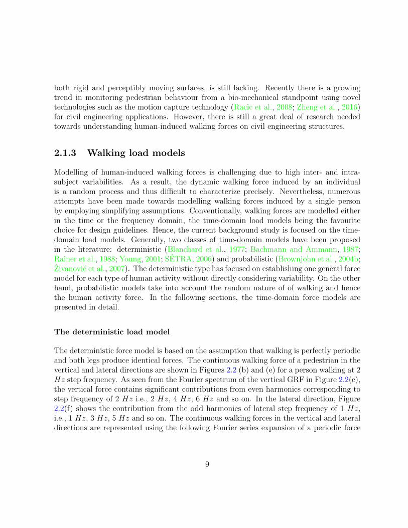
Modelling of human-induced walking forces is challenging due to high inter- and intra-subject variabilities. As a result, the dynamic walking force induced by an individualis a random process and thus difficult to characterize precisely. Nevertheless, numerousattempts have been made towards modelling walking forces induced by a single personby employing simplifying assumptions. Conventionally, walking forces are modelled eitherin the time or the frequency domain, the time-domain load models being the favouritechoice for design guidelines. Hence, the current background study is focused on the time-domain load models. Generally, two classes of time-domain models have been proposedin the literature: deterministic (Blanchard et al., 1977; Bachmann and Ammann, 1987;Rainer et al., 1988; Young, 2001; SETRA, 2006) and probabilistic (Brownjohn et al., 2004b;Zivanovic et al., 2007). The deterministic type has focused on establishing one general forcemodel for each type of human activity without directly considering variability. On the otherhand, probabilistic models take into account the random nature of of walking and hencethe human activity force. In the following sections, the time-domain force models arepresented in detail.

The deterministic load model

The deterministic force model is based on the assumption that walking is perfectly periodicand both legs produce identical forces. The continuous walking force of a pedestrian in thevertical and lateral directions are shown in Figures 2.2 (b) and (e) for a person walking at 2Hz step frequency. As seen from the Fourier spectrum of the vertical GRF in Figure 2.2(c),the vertical force contains significant contributions from even harmonics corresponding tostep frequency of 2 Hz i.e., 2 Hz, 4 Hz, 6 Hz and so on. In the lateral direction, Figure2.2(f) shows the contribution from the odd harmonics of lateral step frequency of 1 Hz,i.e., 1 Hz, 3 Hz, 5 Hz and so on. The continuous walking forces in the vertical and lateraldirections are represented using the following Fourier series expansion of a periodic force

9

(Blanchard et al., 1977):

P (t) =

{G+

∑ni=1Gαv,i sin(i2πfst+ φv,i))∑n

i=1 Gαl,i sin(i2πtfs2

+ φl,i))(2.1)

where, P (t) is the human-induced continuous ground reaction force, G is the pedestrianweight, αv,i and αl,i are the dynamic load factors (DLF) of the ith harmonic in the vertical(v) and lateral (l) directions respectively, and fs is the pedestrian step-frequency (Hz).φv,i and φl,i are the phases of the ith harmonic in the respective directions.

Over time, many researchers have attempted to quantify DLFs based on direct or indi-rect force measurements. The earliest work on this aspect was by Blanchard et al. (1977).The authors proposed a model with one harmonic term in Equation 2.1 for the verticaldirection, with the DLF of value 0.257 based on a resonant condition assuming a pedestrianof weight G equal to 700N. This work is extensively used by the Canadian Highway Bridgecode (CAN/CSA S6, 2011) and the British Standard (BS 5400, 1978) to design PBs. Theirmodel considered that resonance would occur in the first vibration mode due to the firstharmonic of the dynamic load. This DLF was applied to PBs with vertical frequenciesupto 4 Hz, and reduction factors were applied to this value for bridges with frequenciesin the range of 4 Hz to 5 Hz. Later on, Bachmann and Ammann (1987) proposed fiveand two harmonics, respectively, to model the vertical and lateral walking forces. Theyproposed DLF values for the first harmonic of the vertical force ranging between 0.4 atfrequency 2.0 Hz and 0.5 at 2.4 Hz, with linear interpolation for other frequencies withinthis range. They also suggested identical DLFs for the second and third harmonics equalto 0.1, for step frequencies near 2 Hz. They proposed a DLF value of 0.1 for the firsttwo harmonics in the lateral direction. In 1988, Rainer et al. (1988) confirmed the strongdependency of DLFs on the walking frequency based on measured continuous forces for asingle pedestrian. They proposed values for the first four DLFs as shown in Figure 2.3.However, this work lacked statistical reliability due to the limited number of test subjectsand trials. Kerr Kerr (1998) attempted to overcome these shortcomings and proposed sim-ilar values for DLF based on 1000 force measurements on 40 test subjects.Following theseworks, Young (2001) proposed statistical mean values for DLFs for the four harmonics ofthe vertical force as a function of the walking frequency fs as follows:

α1 = 0.37(fs − 0.95) ≤ 0.5

α2 = 0.054 + 0.0044fs

α3 = 0.026 + 0.0050fs

α4 = 0.010 + 0.0051fs

φi = 0 (2.2)

10

where, α1 to α4 are the first four harmonics and φi is the phase for the ith harmonic. Thisis the first work where the stochastic behaviour of human walking has been taken intoaccount in the estimation of DLFs. A brief outline of these efforts in estimating the valuesof DLF values is presented in Table 2.1 and Figure 2.4.

Figure 2.3: Dynamic load factors (DLFs) for first four harmonics of walking (taken fromRainer et al. (1988))

It should be stressed that the DLFs were obtained by direct or indirect force mea-surements on rigid surfaces. However, in the context of civil engineering applications, theflexibility of the walking surface has impact on the walking force and hence the DLF val-ues. Pimentel (1997) found from measurements of structural responses on two full-scalePBs that the first and second resonant vertical harmonics were lower than those givenin literature, which was probably due to human-structure interaction. It should also bestressed that all of the aforementioned studies deal with a single pedestrian. It is imprac-tical to measure the walking-induced loads for groups of people through the experimentalset-ups used. Very few studies on quantifying the effect of crowd on the DLF values existin the literature. Ellis (2003) found through the measured structural responses on a floorunder a group of pedestrians that DLF values decrease as the size of the group increases.Pernica (1990) also reported similar phenomena. These studies point towards imperfectsynchronization within the group leading to a dynamic decrease in the DLF values. Theeffect of multiple pedestrians or crowd and corresponding synchronization phenomena arediscussed later on.

11

Figure 2.4: Dynamic load factors (DLFs) reported in the literature (taken from Willfordet al. (2006))

12

Table 2.1: Summary of proposed DLF values reported in the literatureResearchers DLF Direction Step frequency

(Hz)Blanchard et al. (1977) α1 = 0.257 Vertical < 4Bachmann and Ammann (1987) α1 = 0.4− 0.5, Vertical 2.0− 2.4

α2 = α3 = 0.1Schulze (1980) α1 = 0.37,α2 = 0.10, Vertical 2.0(after α3 = 0.12, α4 = 0.04,Bachmann and Ammann (1987)) α5 = 0.08

α1 = 0.039, α2 = 0.010, Lateralα3 = 0.043, α4 = 0.012,α5 = 0.015

Rainer et al. (1988) Figure 2.3 VerticalAllen and Murray (1993) α1 = 0.50, α2 = 0.20, Vertical 1.6− 2.4

α3 = 0.10, α4 = 0.05Bachmann et al. (1995) α1 = 0.4/0.5, α2 = 0.10 2.0

α3 = 0.10 Vertical 2.0α1 = 0.10 Lateral

Kerr (1998) α1 in Figure 2.4 Verticalα2 = 0.07, α2 = 0.10

Young (2001) Equation 2.2 Vertical 1− 2.8

Probabilistic descriptions for load model parameters

It is unlikely for a person to produce exactly the same walking force in repeated trials,which is known as intra-subject variability. This is even more unlikely for multiple persons,which is known as inter-subject variability. Therefore a probability based approach tomodel walking force is more appropriate than a deterministic approach. Uncertaintiescan be incorporated into the periodic load model in Equation 2.1 through probabilitydistributions for force amplitude, time-frequency parameters of walking and time delaybetween several persons walking. This section reviews the existing probability distributionsfor step frequency, walking velocity and step length.

The work by Matsumoto et al. (1978) was the earliest one to report the statistics ofstep frequencies based on a sample of 505 persons walking at self-selected speeds. Theyrecommended a normal distribution for step frequency with a mean and standard deviationof 1.99 Hz and 0.173 Hz, respectively. Later on, similar research towards estimating

13

the statistics of step frequencies yielded varying statistics, as listed in Table 2.2 (Kramerand Kebe, 1980; Kerr, 1998; Pachi and Ji, 2005; Zivanovic, 2006; Kasperski and Sahnaci,2007). Figure 2.5 shows the normal density function proposed by different authors for stepfrequency. Zivanovic (2006) explained these discrepancies arising due to a wide rangingfactors including gender. In their work, Pachi and Ji (2005) found a linear relationshipbetween walking speed and step frequency from 800 measurements for 100 men and 100women:

v = Lsfs (2.3)

where v is the walking speed of the person, fs is the step frequency and Ls is the average steplength of 0.71 m. Based on the data collected by Pachi and Ji (2005), Zivanovic (2006)showed that the walking velocities follow normal distribution at a specific frequency ofwalking as shown in Figure 2.6. In the study by Zivanovic et al. (2007), the step length ofthe people crossing the bridge was also measured and found to be normally distributed witha mean value of 0.71 m and a standard deviation of 0.071 m. Furthermore, they found thatthe step length was independent of step frequency, which is contrary to one of the earliestfindings by Wheeler (1982) on the correlation between step length and frequency. In orderto investigate the relationship between walking parameters such as speed, step length, andstance period, a comprehensive biomechanical study by taking gender into considerationwas undertaken by Yamasaki et al. (1991). They reported a nonlinear relationship betweenwalking speed and step length, which adds to the confusion from previous studies.

Table 2.2: Statistics os step frequency by different researchersAuthors Mean (Hz) Standard Deviation (Hz)Matsumoto et al. (1978) 1.99 0.173Kerr (1998) 1.9 —Kramer and Kebe (1980) 2.2 0.3Pachi and Ji (2005) 1.8 0.13Zivanovic (2006) 1.87 0.186Kasperski and Sahnaci (2007) 1.82 0.12

Besides the time-frequency parameters for walking, force amplitude is also anotherimportant parameter to model. When modelling the human walking force in the time-domain, the force amplitude (Gαm) is usually defined as the portion of pedestrian’s weighti.e., product of dynamic load factor (DLF or αm) and pedestrian’s body weight (G). Gener-ally, the weight of the pedestrian is treated as a random variable. Wheeler (1982) assumed

14

a distribution of weights obtained for the Australian population. In their probabilisticmodeling framework, Zivanovic et al. (2007) did not consider any uncertainties from G.Later on, Pedersen (2012) conducted a parametric study to investigate the sensitivity ofthe 95th percentile response of a bridge to a stochastic model of pedestrian weight. Theyreported that the response is not very sensitive to whether a stochastic or deterministicmodel is assumed for G, however, it is sensitive to the mean value of the weight used.

1 1.5 2 2.5 3fs (Hz)

0

0.5

1

1.5

2

2.5

3

3.5

PDF

Matsumoto et al., 1978Kramer and Kebe, 1980Pachi and Ji, 2005Zivanovic, 2006Kasperski and Sahnaci, 2007

Figure 2.5: Distribution of step frequency for normal walking

Apart from the weight of pedestrian, significant scatter is also found in the DLF values.The most extensive research to statistically characterize the DLF was conducted by KerrKerr (1998). From 1000 force records on 40 test subjects, the mean DLF for the firstharmonic as a function of step frequency is given by:

µα = −0.2649f 3s + 1.3206f 2

s − 1.7597fs + 0.7613 (2.4)

Under the assumption that the DLFs are normally distributed around their mean value(for a certain walking frequency), the COV was found to be 0.16 (Zivanovic, 2006). Kerrobserved large scatter in the DLF values corresponding to higher harmonics, with a COVof 0.40. Galbraith and Barton (1970) showed an interdependence between G and αm,however, they could not quantify this dependency and assumed that the two variables areindependent.

15

0.9 1 1.1 1.2 1.3 1.4 1.5 1.6Walking speed (m/s)

0

10

20

30

40

50

60

Num

ber

of o

ccur

ence

s

Experimental dataTheoretical

Figure 2.6: Distribution of walking speeds at 1.8 Hz (reproduced from Zivanovic (2006))

These probability density functions of the loading parameters can be used in a probability-based framework to predict a certain level of vibration response. The work by Ebrahimpouret al. (1996) was one of the earliest to include this randomness into modelling forces. Theyincluded the probability distribution function of the time delay between several pedestriansand determined the DLF for the first harmonic under groups of pedestrians. However, theydid not provide a comprehensive force model that can be used to predict the structuralresponse. The first work on estimating the vertical response of a PB through incorporatingthe probability density functions of the loading parameters in a novel probabilistic frame-work was proposed by Zivanovic (2006). However, the methodology is only limited to asingle harmonic. Later on, Zivanovic et al. (2007) extended this probability-based modelto cover not only the main harmonics of the walking force, but also the sub-harmonics,which appear in the frequency domain. A more advanced stochastic load model in thevertical direction was proposed by Racic and Brownjohn (2011) through a comprehensivedatabase of measured continuous vertical walking loads from an instrumented treadmill.Their procedure can simulate random walking force signal from a given step frequency andwalking period.

Although the probabilistic framework incorporates the intra-and inter-subject vari-abilities in walking forces, the main shortcoming of this modelling approach is that it isnumerically cumbersome. As a result, it has not been adopted by practitioners, who still

16

resort to the simplified deterministic load model.

Biomechanical load model

An emerging trend is to model the dynamics and biomechanics of walking, which couldpotentially allow for better characterization of the dynamic forces induced and also toquantify human-structure interaction (Willford, 2002; Brownjohn et al., 2004b; Zivanovicet al., 2010). In this context, mainly two classes of models have been proposed in theliterature. The first category is linear oscillator-based, with single or multiple lumpedmasses connected together with linear springs and dampers. Such models are known asthe spring-mass damper (SMD) models. The second category are biomechanically-inspiredmodels, which were developed originally to simulate walking gait, realistically.

Archbold et al. (2005) used an single-degree-of-freedom (SDOF) SMD model of a singlepedestrian walking across a PB by using parameters selected from the biomechanics liter-ature, which were developed for standing and running actions. Kim et al. (2008) adopteda two-degree-of-freedom SMD model for simulating a single pedestrian walking on a 99 mlong cable-stayed PB (Figure 2.7(a)). Caprani et al. (2011) developed the SDOF SMDmodel by adding a contact force to the model. They reported that their model responseestimates were considerably lower compared to force-only simulations near resonant condi-tions. However, their work lacks experimental validation. A few attempts have been madesince then to identify the bio-dynamic parameters in the context of civil engineering appli-cations. The work of Silva and Pimentel (2011) is one such example, where the parametersof a SDOF SMD walking human model were identified through analyzing the correlation ofwalking force and accelerations of the human body centre of mass (CoM) recorded at thewaist of the subject. Later on, da Silva et al. (2013) developed this model for multi-persontraffic and reported a reduction in the natural frequency of the structure along with anincrease in damping, which also intensified with an increase in the traffic size.

Inverted-pendulum models from the biomechanics literature have also been used exten-sively to simulate the interaction of walking pedestrians with PBs. In such models, the twolower limbs of a human are modelled, known as bipedalism. Bocian et al. (2012) proposeda bipedal model in which human walk is modelled using an inverted pendulum (Figure2.7(b)) and the bridge motion perturbed the gait in the lateral direction. Later on, thiswork was extended to a vertically oscillating bridge Bocian et al. (2013), where the motionof the bridge modified the passive motion of the pedestrian’s centre of mass. However,the inverted pendulum cannot model the double-support phase of walking and ignores thecompliant leg behaviour. Furthermore, their model also did not provide experimental val-idation, specifically in adequately capturing the GRF on a flexible platform. Qin et al.

17

(2013) adopted a bipedal walking model with damped compliant legs to simulate walkingon a vibrating beam as shown in Figure 2.7(c). The dynamic analysis could incorporatehuman-structure interaction as well as bipedal mechanism of walking. However, too manyparameters makes this model overly complex. Their research, moreover, did not includeany experimental validation studies to support their modelling assumptions.

Figure 2.7: (a)Two degree of freedom SMD model as adopted by Kim et al. (2008), (b)inverted pendulum model as adopted by Bocian et al. (2012) and (c) bipedal-walking modelas adopted by Qin et al. (2013)

Modelling crowd effect

Since the serviceability problems of PBs are exacerbated by groups of pedestrians or crowds,quantifying crowd-induced loads is essential for vibration serviceability assessment of PBs.All of the aforementioned studies on modelling walking load from measurements using forceplates or instrumented treadmills deal with a single pedestrian. Similar studies for groups ofpeople do not exist. Modelling crowd effect has been conducted so far by extrapolating theeffect of single pedestrian through a multiplication factor. The first attempt at modellingrandom loads induced by a group of N pedestrians was conducted by Matsumoto et al.(1978). Assuming pedestrian arrival at the bridge follows a Poisson distribution, theystochastically superimposed individual responses to predict the total response. It wasfound that the total response can be obtained by multiplying a single pedestrian responseby a multiplication factor,

√N or λT0, where λ is the mean arrival rate of pedestrians

(number of pedestrians/second/width), and T0 stands for the elapsed time to cross the

18

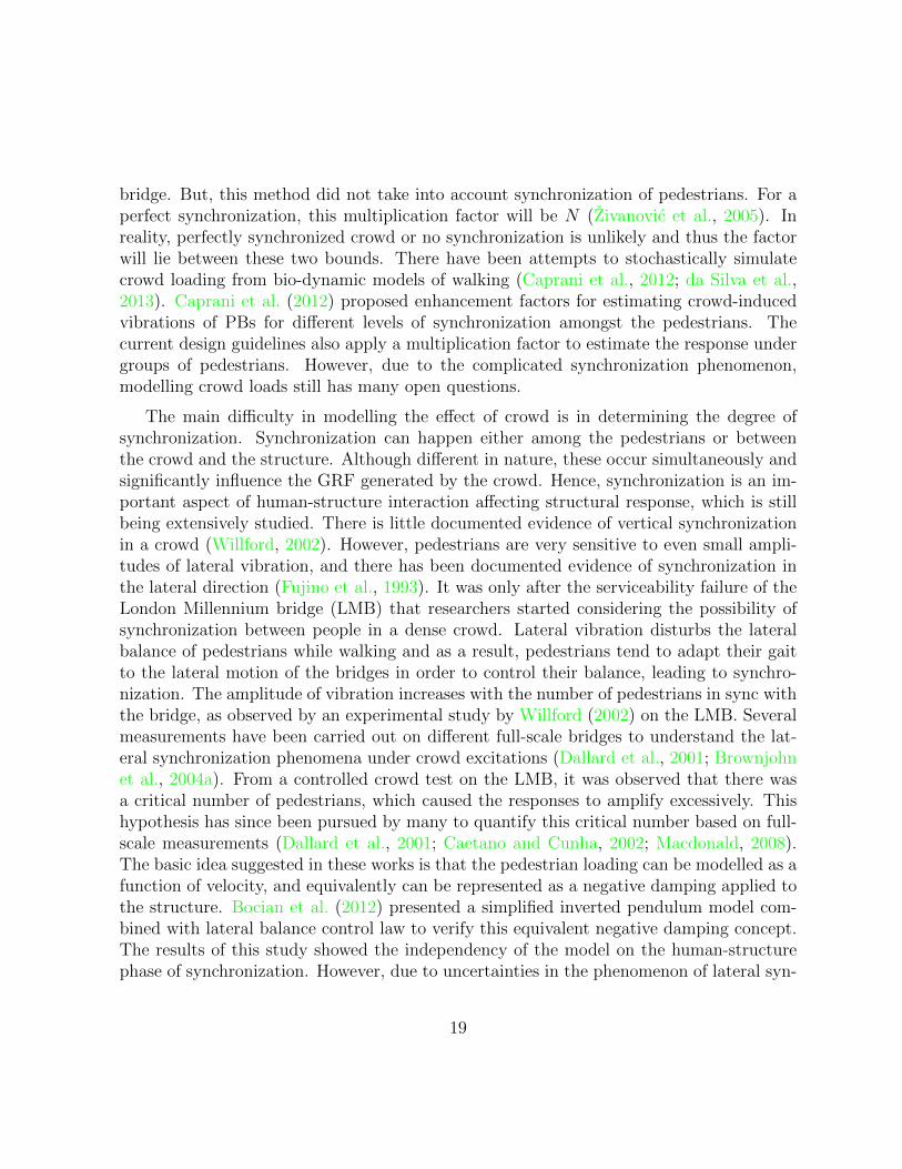
bridge. But, this method did not take into account synchronization of pedestrians. For aperfect synchronization, this multiplication factor will be N (Zivanovic et al., 2005). Inreality, perfectly synchronized crowd or no synchronization is unlikely and thus the factorwill lie between these two bounds. There have been attempts to stochastically simulatecrowd loading from bio-dynamic models of walking (Caprani et al., 2012; da Silva et al.,2013). Caprani et al. (2012) proposed enhancement factors for estimating crowd-inducedvibrations of PBs for different levels of synchronization amongst the pedestrians. Thecurrent design guidelines also apply a multiplication factor to estimate the response undergroups of pedestrians. However, due to the complicated synchronization phenomenon,modelling crowd loads still has many open questions.

The main difficulty in modelling the effect of crowd is in determining the degree ofsynchronization. Synchronization can happen either among the pedestrians or betweenthe crowd and the structure. Although different in nature, these occur simultaneously andsignificantly influence the GRF generated by the crowd. Hence, synchronization is an im-portant aspect of human-structure interaction affecting structural response, which is stillbeing extensively studied. There is little documented evidence of vertical synchronizationin a crowd (Willford, 2002). However, pedestrians are very sensitive to even small ampli-tudes of lateral vibration, and there has been documented evidence of synchronization inthe lateral direction (Fujino et al., 1993). It was only after the serviceability failure of theLondon Millennium bridge (LMB) that researchers started considering the possibility ofsynchronization between people in a dense crowd. Lateral vibration disturbs the lateralbalance of pedestrians while walking and as a result, pedestrians tend to adapt their gaitto the lateral motion of the bridges in order to control their balance, leading to synchro-nization. The amplitude of vibration increases with the number of pedestrians in sync withthe bridge, as observed by an experimental study by Willford (2002) on the LMB. Severalmeasurements have been carried out on different full-scale bridges to understand the lat-eral synchronization phenomena under crowd excitations (Dallard et al., 2001; Brownjohnet al., 2004a). From a controlled crowd test on the LMB, it was observed that there wasa critical number of pedestrians, which caused the responses to amplify excessively. Thishypothesis has since been pursued by many to quantify this critical number based on full-scale measurements (Dallard et al., 2001; Caetano and Cunha, 2002; Macdonald, 2008).The basic idea suggested in these works is that the pedestrian loading can be modelled as afunction of velocity, and equivalently can be represented as a negative damping applied tothe structure. Bocian et al. (2012) presented a simplified inverted pendulum model com-bined with lateral balance control law to verify this equivalent negative damping concept.The results of this study showed the independency of the model on the human-structurephase of synchronization. However, due to uncertainties in the phenomenon of lateral syn-

19

chronization, more experimental results from real case studies are required to verify thesehypotheses.

2.1.4 Limitations of existing walking load models

Despite numerous attempts to characterize and model pedestrian-induced walking forces,as discussed in the previous sections, there are clear shortcomings in the existing walkingload models, which are summarized below:

• In general, nearly all walking load models are based on force measurements, obtainedfrom either force plates on rigid ground or instrumented treadmills in artificial lab-oratory conditions. However, in the context of civil engineering applications, theflexibility of the walking surface has an effect on the induced force due to human-structure interaction. Although several attempts have been made recently to monitorwalking behaviour through novel technologies such as the motion capture technologyfor civil engineering applications, conclusive results are still not available. Thus, agreat deal of research needs to be dedicated towards understanding human-inducedwalking forces on flexible structures.

• The traditional deterministic load models do not take into account intra-subject vari-ability. Although, the probabilistic models incorporate both intra-and inter-subjectvariabilities in walking forces, the main shortcoming of this modelling approach isthat it is computationally intensive. As a result, probabilistic models have not yetbeen adopted by practitioners, who rely on simplified deterministic load models.

• Although the bio-mechanical models attempt to account for human structure inter-action, too many model parameters and the absence of generally applicable valuesof biodynamic properties of human body model make these models difficult to ap-ply in design situations. Moreover, experimental studies employing these models arelacking.

• The difficulty in characterizing crowd-induced walking excitation is in determiningthe degree of synchronization within the pedestrians as well as between the structureand the pedestrians. Due to uncertainties in the phenomenon of synchronization,experimental results from real case studies are required to investigate and quantifythis phenomenon.

20

2.2 Vibration serviceability design of PBs

In the serviceability-based design of PBs, a simple predictive model of the pedestrian-induced walking force, the dynamic properties of the structures, and the desired accelera-tion limits for human comfort are the key required elements. Early research into vibrationserviceability of PBs dates back to the seventies, with the work of Blanchard et al. (1977)to define design guidelines for the assessment of human-induced vertical vibrations of PBs.His work was later incorporated into several international bridge design codes (BS 5400,1978; CAN/CSA S6, 2011). Although the effect of multiple pedestrians has been well ap-preciated in the seventies (Matsumoto et al., 1978; Wheeler, 1982), only a simplified singlepedestrian load scenario was included in the standards. Over the years, several codes andguidelines has been developed to calculate the vibration response to multi-person trafficby multiplying the response due to a single person excitation with a factor. This approachoriginated from the work of Matsumoto et al. (1978) and is adopted by the existing designguidelines due to its simplicity. However, most of the design guidelines consider a rangeof multiplicative factors, not the values originally suggested by Matsumoto et al. (1978).As the serviceability issues of PBs is exacerbated in crowd scenarios and generally governsthe design case, the current study is limited to the vibration serviceability design undergroup/crowd loading conditions, which covers ISO 10137, Eurocode 5, British nationalAnnex to Eurocode 1 and SETRA. The four design guidelines (see Table 2.3) are discussedin detail in the following sections.

2.2.1 A two-step approach

In general, all the design guidelines ensure serviceability in a two-step approach. In the firststep, the structural frequency is checked to see if it falls outside a critical frequency ranges,prescribed by the guidelines. If the structural frequency falls above the prescribed criticalvalues, the structure is deemed to automatically satisfy the serviceability requirements.However, if the structural frequency falls below these critical values, the serviceability is metthrough limiting the structural vibrations to specified acceleration levels. For this purpose,a detailed dynamic analysis should be performed, following which the predicted accelerationresponse is compared with the vibration limit in order to ensure desired comfort to thepedestrians on the bridge.

In the first step, restricting the structural frequency outside the critical frequency limitsensures that the serviceability requirements are satisfied. These frequency limits are pro-posed by the guidelines in order to take care of the walking harmonics potentially resonating

21

with the dominant structural modes of vibration. Keeping the structural frequency outsidethe critical ranges avoids the possibility of excessive vibrations under resonant conditions.Table 2.3 lists the critical values of frequency suggested by the guidelines. As shown inthe table, these frequency ranges are not consistent across provisions. Some criteria limitthe frequency in the vertical direction to 5 Hz (EN 1995-2, 2004; SETRA, 2006), whichconsiders the possibility of resonance up to the second harmonic of the walking frequency(≈4.8 Hz). Only the British National Annex considers up to three harmonics by assumingthe critical frequency limit at 8 Hz. Although ISO 10137 explicitly does not provide anylimit on the frequency, it considers up to five harmonics of walking frequency and thus,implicitly defines a critical range of 1.2 Hz to 12 Hz. Similarly in the lateral direction,the frequency limit is 2.5 Hz in most of the guidelines, aimed at capturing up to twoharmonics, except the British National Annex which limits to 1.5 Hz.

Table 2.3: Limiting frequencies proposed by different design guidelines

CodeLimit frequency in HzVertical lateral

ISO 10137 (implicit) 1.2− 12 1.2Eurocode 5 < 5 < 2.5British Annex to Eurocode 1 < 8 < 1.5

SETRA 1− 5 0.3− 2.5

In the second step of serviceability assessment, it is ensured that the bridge responsesestimated through a dynamic analysis meet the desired comfort limits. The comfort limitsfor pedestrians are generally specified in terms of peak acceleration, except for ISO 10137,which uses the root mean square (RMS) value (1 second average) of accelerations. ISO10137 provides base curves as shown in Figure 2.8, which are multiplied by a factor of 60for the RMS acceleration in both the vertical and lateral directions. It is worth noting thatthe acceleration limit in the lateral direction does not extend below 1 Hz, while a lateralfundamental frequency below 1 Hz could also be important, as evidenced by the LMB.The peak acceleration limits specified by other guidelines are listed in Table 2.4. WhileEurocode 5 and ISO 10137 propose a single comfort limit, other codes have proposeddifferent limits based on site usage, height of the structure, traffic class or the level ofcomfort. The British National Annex proposes the following acceleration limit:

alim = 1.0k1k2k3k4 with 0.5 ≤ alim ≤ 2.0 m/s2 (2.5)

where, k1 is the site usage factor with values ranging between 0.6 to 1.6 based on theintended bridge function; k2 is the route redundancy factor with values ranging from 0.7

22

to 1.3; k3 is the height factor with values from 0.7 to 1.1; k4 is the exposure factor and istaken as 1.0 unless specified. The limits proposed by ISO 10137 are frequency dependent,while others are independent of frequency. This implies that the limits are applicable onlywithin the specified frequency range in Table 2.3, as specified by the respective guidelines.With the exception of ISO 10137, which offers guidance on the limits until 80 Hz, othersdo not offer guidance for structural frequencies above 5 or 8 Hz.

Table 2.4: Acceleration limits specified in guidelines

CodesLimit acceleration in m/s2

Vertical LateralEurocode 5 0.70 0.20 for single pedestrian,

0.4 for crowd loadingBritish National 0.5− 2.0 (Equation 2.5) –Annex to depending on site usage,Eurocode 1 route redundancy and

height of structure

SETRAMaximum comfort: < 0.5 (Limit I) < 0.1 (Limit I)Average comfort: 0.5 (Limit I) − 1.0 (Limit II) 0.1 (Limit I) − 0.3 (Limit II)Minimum comfort: 1.0 (Limit II) − 2.5 (Limit III) 0.3 (Limit II) − 0.8 (Limit III)Unacceptable: > 2.5 (Limit III) > 0.8 (Limit III)

2.2.2 Dynamic analysis

In the second step of the serviceability assessment, a dynamic analysis may be requiredfor PBs with natural frequencies (vertical or lateral) within the critical values listed inTable 2.6. For this analysis, the design guidelines assume resonant conditions, where thestructure is assumed to be excited at its natural frequency by the pedestrians. Eitherthe SDOF (single degree of freedom) approach for simple structures or the finite elementmethod for complex systems are recommended for response prediction by the guidelines.A detail review of the response prediction by the guidelines is presented below.

ISO 10137

The ISO 101317 (ISO 10137, 2007) guideline is published by the International Organisationfor Standardization, and can be used for vibration serviceability design of buildings and

23

pedestrian walkways. This guideline provides some scenarios to consider during such anassessment:

• one person walking across the bridge;

• average pedestrian flow for groups of between 8 and 15 people;

• streams of pedestrians for groups of significantly more than 15 people, and

• the occasional festive or choreographic event if relevant.

100

101

102

10−3

10−2

10−1

Frequency (Hz)

RM

S A

ccel

erat

ion

(m/s2 )

100

101

102

10−3

10−2

10−1

100

(a) (b)

Figure 2.8: Base curves in accordance to ISO 10137 for (a) vertical and (b) lateral directions

ISO 10137 describes the dynamic actions of one or more people by the use of a time-domain moving load model, which is expressed using a Fourier series approximation. Theforce due to a single pedestrian in both the lateral and vertical directions can be writtenas (Allen and Murray, 1993):

Fd(t) = Q(1 +k∑

m=1

αm,d sin(2πmfdt+ φm,d)) (2.6)

where, αm,d and φm,d are, respectively, the dynamic load factor (DLF) and the phase anglecorresponding to the mth harmonic in the direction under consideration (the subscript d

24

stands for direction, vertical or lateral). Q is the total static load of the participatingpedestrians and fd is the frequency of walking in the direction under consideration. Thelateral frequency is one-half of the vertical frequency. Other design parameters such as thestep frequency and DLF to estimate the forces due to one person are listed in Table 2.5.

Table 2.5: Design parameters for moving forces due to one person according to ISO10137.2007

Harmonic number, Range of frequency, Numerical coefficientn f αn,v αn,h1 1.2 to 2.4 0.37(f − 1.0) 0.12 2.4 to 4.8 0.13 3.6 to 7.2 0.064 4.8 to 9.6 0.065 6.0 to 12.0 0.06

ISO 10137 states that the dynamic actions of group of pedestrians depends primarilyon the weight of the participants, the maximum density of persons per unit floor area,and on the degree of coordination among the pedestrians. The coordination is taken intoaccount by applying a coordination factor, C(N), to the forcing function in Equation 2.6:

F (t)N = Fd(t)C(N) (2.7)

If the movement of the group is uncoordinated, the coordination factor is√N/N . It is easy

to see the similarity between this coordination factor and the√N multiplier in (Matsumoto

et al., 1978) if we think of Q in Equation 2.6 as a product of N and the average weight ofthe pedestrians in a group (G). A conservative approach for the phase angle is obtainedby introducing a phase shift of 90◦ for harmonic contributions below resonance.

Eurocode 5

Eurocode 5 (EN 1995-2, 2004) was developed in the U.K. in 2004, specifically for the designof timber bridges. However, the response model defined is not specific to any material andtherefore, could be used for PBs in general. Moreover, this code assumes the PB to bea simply supported beam or a truss system. Unlike ISO 10137, it provides the equationto estimate the maximum acceleration response of PBs under N pedestrians. A value ofN = 13 for distinct groups and 0.6A for a continuous stream of pedestrians is suggestedfor design, where A is the bridge deck area in m2. According to this standard, the vertical

25

acceleration of the bridge due to N pedestrians, av,n in m/s2, is given by:

av,n = 0.23av,1Nkvert (2.8)

where av,1 is the response under single pedestrian and given by,

av,1 =

{200Mζ

for fv ≤ 2.5100Mζ

for 2.5 < fv ≤ 5.0(2.9)

Similarly, the lateral acceleration ah,n in m/s2 is calculated using:

ah,n = 0.18ah,1Nkhor (2.10)

where, ah,1 is the lateral acceleration in m/s2 for one person crossing the bridge and cal-culated using:

ah,1 =50

Mζfor 0.5 ≤ fh ≤ 2.5 (2.11)

In these equations, M is the total mass of the bridge, ζ is the damping ratio, fv and fh arethe vertical and lateral natural frequencies of the structure, respectively, and kvert and khorare coefficients according to Figure 2.9 (a) and (b) and N is the number of pedestrians.Although this guideline uses a response based model as opposed to a force model, equations2.9 and 2.11 are in fact a result of the basic moving load model (Equation 2.1) underresonant condition, while using different values for the dynamic load factor (Butz, 2008).These formulae given are based on the following parameters:

• the weight of the pedestrian is 700 N;

• the DLF in the vertical directions are 0.45 and 0.22 respectively for first and secondharmonics and 0.10 in the lateral direction for the first two harmonics, and

• a reduction factor of 0.63 is applied to take care of the reduction due to the pedes-trian’s movement in the longitudinal space.

The factor 0.23 in Equation 2.8 accounts for the synchronization probability of the groupof pedestrians crossing the bridge, and the factor 0.18 in Equation 2.10 accounts for thehorizontal lock-in probability for the group of pedestrians crossing the bridge. The coef-ficients kvert and khor account for the risk of resonance that the step frequencies coincidewith the natural frequency of the bridge.

26

0 1 2 3 4 5Vertical mode (Hz)

0

0.2

0.4

0.6

0.8

1k ve

rt

0 0.5 1 1.5 2 2.5Lateral mode (Hz)

0

0.2

0.4

0.6

0.8

1

k hor

(a) (b)

Figure 2.9: (a) Vertical and (b) lateral response reduction factors in accordance withEurocode 5

British National Annex to Eurocode 1

The British National Annex (NA to BS EN 1991-2, 2003) classifies PBs into four categories:

• Class A: rural locations, which are seldomly used (2 P or 0 P/m2);

• Class B: location with occasional variations in the pedestrian loading intensity (4 Por 0.4 P/m2);

• Class C: urban routes subject to significant variation in the daily usage (8 P or 0.8P/m2);

• Class D: primary access to major public assembly (16 P or 1.5 P/m2).

Three load models are proposed based on these classifications. Two of these models con-sider the vertical direction, while the third considers the lateral direction. The maximumvertical acceleration under a group of N pedestrians walking is estimated by assuming amoving vertical force (F in N) at constant speed, which is given by:

F = F0k(fv)√

1 + γ(N − 1) sin(2πfvt) (2.12)

where, F0 is the moving force amplitude of 280 N for a pedestrian weight of 700 N; k(fv),which is a function of the vertical natural frequency (fv) in Figure 2.10(a) is a combination

27

factor to deal with: (a) the effect of more realistic pedestrian population, i.e., equivalentnumber of pedestrians, (b) harmonic response, and (c) relative weighting of pedestriansensitivity to response; γ is a factor to allow for the unsynchronized combination of actionsin a pedestrian group and is obtained from Figure 2.10(b); N is the number of pedestrianswho are assumed to cross the bridge together in a group. With force amplitude F0 being280 N , it is clear that this guideline considers a uniform DLF of 0.4 for all the first threeharmonics. The reduction in response due to second and third harmonics (α2 and α3) isaccounted through k(fv) in Figure 2.10(a). The DLFs for these higher harmonics can beobtained through the function k(fv) by normalizing the maximum value of k(fv) in thesecond (2.8 ≤ fv < 5.6) and third harmonic regions (5.6 ≤ fv < 8.0) to 1.0. The α2 andα3 values so obtained are, respectively, 0.14 and 0.051 with normalized k(fv), denoted byk′(fv)

0 2 4 6Vertical mode (Hz)

0

0.5

1

1.5

k(f v)

0 0.05 0.1 0.15 0.2Logarithmic Decrement

0

0.5

1

1.5

γ

Group of 10Group of 15Group of 20)Dense crowd

0 5 10 15Lateral mode (Hz)

0

0.5

1

1.5

2

D

Stable

(a) (b)

Unstable

(c)

Figure 2.10: (a) Vertical response reduction factor, (b) reduction factor γ as a function ofthe logarithmic decrement, and (c) the damping factor as a function of the lateral modeby the British National Annex

28

The second modelling approach is based on the assumption of continuous flow, wherethe pedestrians are on the bridge for a sufficient amount of time such that steady stateconditions are achieved. In such a scenario, the load is distributed over the entire spanand is given by:

w = 1.8F0

Ak(fv)

√γN

λsin(2πfvt) (2.13)

where, w is the distributed load in N/m2; A is the area of deck in m2; N is the numberof pedestrians in the group, given by ρA; ρ is the crowd density per m2; λ is a factor thatreduces the effective number of pedestrians in proportion to the enclosed area of the modeof interest (for the first mode shape of a simply supported beam, this is equal to 0.634).

This standard does not require a dynamic analysis to assess serviceability in the lateraldirection. This involves calculating the damping parameter D using:

D =mbridgeζ

mpedestrian

(2.14)

where, mbridge is the mass per unit length of the bridge and mpedestrian is the mass perunit length of pedestrians for the relevant crowd density. The serviceability in the lateraldirection is determined through comparing the parameter D with the stability envelopeas defined in Figure 2.10(c). Instability will occur when the this damping parameter fallsbelow the indicated envelope.

SETRA

The SETRA guideline (SETRA, 2006) of the Technical Department for Transport, Roadsand Bridges Engineering and Road Safety of France (2006) adopts different ranges offrequencies and traffic classes in its design methodology. It has presented three load casesfor pedestrian walking loads: Case 1 for sparse and dense crowd with densities rangingfrom 0.5 - 0.8 pedestrians (P)/m2 ; Case 2 for very dense crowd with densities ≥ 1.0 P/m2;and Case 3 to consider second harmonic effect for an evenly distributed crowd. These loadcases are developed based on four classes of PBs depending on the level of traffic they areexpected to experience:

• Class I: urban PB subjected to very heavy traffic frequently (1.0 P/m2)

• Class II: urban PB with heavy traffic (0.8 P/m2)

• Class III: PB with moderate traffic (0.5 P/m2)

29

• Class IV: PB with low level of traffic (< 0.5 P/m2)

SETRA also proposes four classes of frequency ranges depending on the expected risk ofresonance as reported in Table 2.6. Table 2.7 lists the proposed load cases to considerbased on the traffic dependent bridge classes and frequency ranges.

Table 2.6: Frequency ranges for vertical and lateral vibrationsRanges of frequency Vertical frequency (Hz) Lateral frequency (Hz)

Range 1 1.7-2.1 0.5-1.1Range 2 1-1.7; 2.1-2.6 0.3-0.5; 1.1-1.3Range 3 2.6-5.0 1.3-2.5

Table 2.7: Load cases considered for different fundamental frequency rangesBridge class Range 1 Range 2 Range 3Class I Case 2 Case 2 Case 3Class II Case 1 Case 1 Case 3Class III Case 1 — —

Random loads due to a stream of N pedestrians corresponding to a specific crowddensity (d) are simplified to deterministic loads under equivalent number of pedestrians(neq), which is given by:

neq =

{10.8√ζiN for d < 1.0

1.85√N for d ≥ 1.0

(2.15)

Here, ζi is the ith modal damping factor. To estimate response, the load due to neqpedestrians is assumed to be uniformly distributed on the deck. The distributed load perunit area (A) in any direction (vertical or lateral) is defined as:

p =αGψneq

Acos(2πft) (2.16)

where G is the average weight of the group of pedestrians and α is the DLF, which is0.4 and 0.1 for the first and second harmonics in the vertical direction, respectively and0.05 and 0.01 for the first and second harmonics in the lateral direction, respectively. ψis the reduction factor, which is a function of the structural frequency (Figure 2.11(a) and(b)) and denoted by ψv and ψl in the vertical and lateral directions respectively. f is theexcitation frequency and equals to the structural frequency as the analysis is performed

30

under resonant condition. The uniformly distributed load is applied to the entire bridge.The direction of application of the load is the same as the direction of the mode shape. TheSETRA guideline considers the possibility of resonance in the first and second harmonicsof walking through the factor ψ. The loads are distributed according to the correspondingmode shape to obtain the design response.

SETRA explicitly takes into account the effect of pedestrian weight on the structuralfrequency and predicts two bounds for the peak response; one considers the effect on anempty bridge, while the other is calculated based on the modified structural frequency dueto the weight of pedestrians (uniformly distributed on the deck). The modified frequencyis estimated as:

f ′n =fnρ

(2.17)

where ρ is the influence factor for additional pedestrian mass given by,

ρ =

√µD + µpµD

(2.18)

with µD and µp are the bridge deck and pedestrian mass per unit length of bridge, respec-tively.

1 2 3 4 5

Vertical mode (Hz)

0

0.2

0.4

0.6

0.8

1

1.2

ψv

0.5 1 1.5 2 2.5

Lateral mode (Hz)

0

0.2

0.4

0.6

0.8

1

1.2

ψl

(a) (b)

Figure 2.11: Response reduction factor (ψ) in the (a) vertical and (b) lateral directionsaccordance with SETRA guideline

31

2.3 Structural response simulation under walking loads

A PB can be modelled in terms of mass, damping, stiffness of the bridge, and possiblehuman-structure interaction for the purposes of response simulations. Traditionally, acombination of modal testing and finite element analysis is conducted to estimate themass, damping, and stiffness of bridges. Knowing the modal properties and modelling thesource or the walking force as discussed in the previous section, the well known equationof motion of a multiple-degree-of-freedom (MDOF) system can be formulated as:

Mx(t) + Cx(t) + Kx(t) = f(t) (2.19)

where M, C and K are the mass, damping, and stiffness matrices respectively of n × n,where n is the degrees of freedom of the structure. x(t), x(t), x(t), and f(t) are vectors ofsize n corresponding to acceleration, velocity, displacement, and the force induced by thepedestrian. Assuming that the system is linear and proportionally damped, the given equa-tion of motion can be written in the modal domain as n uncoupled equations representingn equivalent single-degree-of freedom systems:

MnYn + CnYn +KnYn = fn(t) (2.20)

where, Yn(t) is the nth modal displacement response of the system at the time instant tand its first and second derivative represent the velocity and acceleration of the bridgedue to the excitation. Mn, Cn, Kn, and fn(t) represent the nth modal mass, damping,stiffness, and force of the bridge. For response simulation using the periodic load models,the pedestrian is assumed to be moving with an uniform walking speed (Figure 2.12). Themodal force fn(t) is given by:

fn(t) =

∫ L

0

δ(x− vt)φn(x)P (t)dx (2.21)

where P (t) is continuous walking force by a pedestrian while walking at speed of v. φn(x)is the mode shape of the bridge deck. If the bridge deck acts as a simply supported beamof length L, the mode shape of the beam is given by:

φn(x) = sin(nπx

L) (2.22)

where x = vt is the position of moving load at any time t on the beam. v is the walk-ing speed and can be calculated as a function of the pacing frequency using the relation(Zivanovic, 2012):

v = 0.714fs + 0.055 (2.23)

32

Hence, the equation of motion in Equation 2.20 for mode n can be rewritten after substi-tuting the modal load fn(t) as:

MnYn + CnYn +KnYn = (G+m∑i=1

Gαi sin(i2πfs)) sin(nπvt

L) (2.24)

Figure 2.12: Moving load on a simply supported PB

In the case of PBs, the forced phase, i.e., when the pedestrian is on the bridge, aloneis important for serviceability. For the forced phase, the response is simulated from thetime the pedestrian steps onto the bridge to the instant the pedestrian leaves the bridgeat the other end. Hence the total duration required to cross the bridge is T = L/v. Theresponse of the bridge at the mid-span can the be estimated numerically or analytically (seeAppendix A). Generally, the most popular method for establishing and solving Equation2.24 is the finite element (FE) method. However, when one mode dominates, which oftenhappens in PBs, the response can be estimated sufficiently accurately using an SDOFmodal equation for the appropriate mode. This is very often implemented in practicewhen checking PB vibration serviceability using the design guidelines.

2.4 Full-scale experiments on PBs

There have been several full-scale studies on PBs conducted for their performance as-sessment under pedestrian-induced excitations. One of the most extensive experimentalcampaign was carried out on the LMB following the large amplitude motions, which oc-curred during its inauguration day (Dallard et al., 2001), leading to a shutdown. The LMBis a steel suspension bridge with a total span of 332 m and the largest individual span beingat the centre, 144 m in length. It has natural frequencies at 0.48 Hz, 0.78 Hz, 0.95 Hz, and1.05 Hz in the lateral direction and thus falls within the critical ranges of frequencies in

33

the lateral direction with risks of resonance at the first harmonic. It was observed that fora certain number of pedestrians, the bridge response was limited, whereas a small increasein the number of pedestrians (beyond a critical number) often resulted in excessive lateralresponse (Dallard et al., 2001) causing instability to the pedestrians. In 2002, Willford(2002) reported an increase in the damping of the LMB under walking load in the verticaldirection. Subsequently, several other bridges were subjected to field tests for dynamicperformance assessment, most notably, the M-Bridge in Japan (Nakamura, 2003), the steelbridge at Changi airport in Singapore, (Brownjohn et al., 2004a), the Clifton SuspensionBridge in England (Macdonald, 2008), and the Pedro e Ines bridge in Portugal (Caetanoet al., 2010).

The M-Bridge is a suspension bridge with a main span of 320 m, which consists ofa reinforced concrete tower supporting a deck with H-girders, sway bracing, and steelgrating. The critical frequencies were found to be the third mode at 0.88 Hz and the fourthmode at 1.02 Hz, both in the lateral direction (Nakamura, 2003). The Changi MezzanineBridge is a 140 m span flat arch bridge constructed from welded tubular steel sectionsinside a tunnel that connects two passenger terminals at the Changi Airport in Singapore.The modes that can be easily excited by pedestrian movements are: the lateral mode atapproximately 0.9 Hz and the torsional mode at 1.64 Hz. Macdonald (2008) investigatedthe Clifton Suspension Bridge in England. The main span, between centre lines of the piers,is approximately 214 m, with chain side spans each of 59 m. Footways on either side of thedeck, outside the girders, result in a total deck width of 9.46 m between the centre lines ofparapets. The deck is comparatively light, being made of timber with wrought iron latticecross-girders in line with each pair of suspension rods. A total of 27 modes under 3 Hz wereidentified, with most of those modes being either vertical or torsional. The 274 m longPedro e Ines bridge in Portugal is formed by a central parabolic arch with approximately9 m rise and 110 m chord. The deck has a width of 4m and is formed by a L-shapedbox cross section, whose top flange is a composite steel-concrete slab. This bridge mostlyresults in very complex mode shapes, which have coupled lateral and vertical displacements.Caetano et al. (2010) identified a total 10 vibration modes below 3 Hz, which are in therange of pedestrian excitable frequencies. All of these bridges are mostly prone to potentialresonance with the first harmonic of the walking frequencies. The experimental studies ontheses bridges consisted of modal testing using accelerometers as well as walking testswith groups of pedestrians. Mostly, the results from the experiments pointed towardsthe synchronization phenomenon due to human-structure interaction leading to changes intheir modal properties.

Besides these studies, several attempts have been made in the literature to evaluatethe design guidelines through experimental studies on in-service PBs. Pimentel (1997)

34

conducted modal as well as walking tests on three PBs: a single span composite PB withfirst vertical mode at 3.67 Hz, a single span stressed ribbon concrete PB with first twovertical modes at 2.3 Hz and 3.6 Hz, and a three span ACM cable-stayed PB with first twovertical modes at 1.92 Hz and 2.59 Hz. The results from the study highlighted that thedeterministic load models overestimate the response under resonant conditions. Salgadoet al. (2014) conducted single pedestrian walking tests on the timber Gois PB in Portugalwith first lateral vibration mode at 2.46 Hz and concluded that the current codes are notfully applicable to all kind of PBs, particularly when they have frequencies near those,which are considered to have vibration problems. Zivanovic et al. (2010) performed acomparison between the existing design procedures for groups of pedestrians based onexperiments on two full-scale bridges: Reykjavik City pedestrian bridge and Podgoricabridge. The 160 m long Reykjavik City bridge was built as a continuous post tensionedconcrete beam. The first two critical vertical modes of the bridge are at 2.08 Hz and2.33 Hz. The Podgorica bridge of length 104 m is a steel box girder pedestrian bridgewith critical vertical frequency at 2.04 Hz. All these comparison studies conducted sofar are based on low-frequency PBs with risk of resonance with the lower harmonics ofwalking frequency. Experimental studies to assess the performance of bridges with differentdynamic properties, specifically having risk of resonance with the higher harmonics ofwalking frequencies, are still lacking in the literature. Moreover, these full-scale studies arebased on in-service PBs, where it is was not possible to conduct repetitive walking testswith different traffic conditions due to usage restrictions. While there are a few laboratoryplatforms involving prototype bridge specimens, no full-scale studies on lively PBs havebeen conducted to the author’s knowledge in a controlled laboratory environment, withthe exception of this work.

2.5 Gap areas in existing research on vibration ser-

viceability of PBs

For PBs, a large amount of research, as discussed in the previous sections, has been pub-lished in recent years, which broadly focuses on analyzing vertical and lateral pedestrian-induced vibrations. However, several important issues related to their design methodologiesand performance assessment remain unaddressed, or only partially addressed in the liter-ature. A summary of the gap areas in the existing research on vibration serviceability ofPBs is described here under and presents the motivation for the current study:

• Evaluating and improving existing design models for vibration serviceability assess-

35

ment of PBs relies on the availability of experimental data from full-scale PBs with arange of dynamic characteristics. Although several experimental studies on full-scalePBs under walking-induced excitation have been performed, at the moment a com-prehensive experimental data set of walking tests under different traffic conditions onlively PBs that exhibit a potential for resonance with the higher harmonics of walkingfrequency, is not available. Moreover, most of the laboratory experimental studieswere conducted on short walkways instrumented to characterize the walking-inducedGRFs. This may not represent walking on a flexible bridge. Aside from a lack ofexperimental database, there is limited evidence of real case studies to investigatethe human-structure interaction phenomena. Hence developing a comprehensive ex-perimental data base from lively structures, on which the interaction phenomena ismost likely to occur, would significantly contribute in understanding and modellingthis phenomena.

• All design guidelines adopt the periodic moving load model. Although the perfor-mance of such models has been evaluated for resonant cases (with respect to the firstharmonic of the walking frequency), there is still a need to validate these models forstructures that do not resonate with the first harmonic, but with higher harmonicsof walking. Although counter-intuitive at first, such an investigation is important,as the results might show that the design guidelines are un-conservative for the non-resonant cases. Moreover, the frequency characteristics of the simulated response,i.e., contributions from the harmonics of walking frequency as well as the structuralfrequency (transient) have also not been investigated yet.

• Although significant disagreement is observed between measurements and predictionsby the design guidelines in resonance (mostly with the first harmonics of walkingfrequency), no attempts have been made yet in reconciling the shortcomings of thedesign provisions. To be clear, it is to be expected that the serviceability assessmentoutcomes using the guidelines should yield conservative values, but they should alsobe balanced so that they are economical.

• Uncertainties in the arrival time, pacing frequency, step length, and weight have al-ready been accounted for in developing design provisions such as SETRA and theBritish National Annex to Eurocode 1. However, the sensitivity of various service-ability assessment methodologies to the uncertainties from the structural proper-ties or the human perception levels to structural motion have not yet been studied.Moreover, none of the existing guidelines have been evaluated in a reliability-basedframework.

36

2.6 Specific objectives

Based on the identified gaps in the literature, the specific objectives of this thesis are thefollowing:

• develop a comprehensive experimental test program on full-scale pedestrian bridgesencompassing different dynamic characteristics with particular focus on PBs thatresonate with the higher harmonics of walking frequency;

• assess the performance of the conventional load model adopted by all the existing de-sign guidelines in predicting the structural response under single-pedestrian walkingfor resonant as well as non-resonant scenarios through the experimental study;

• evaluate the most popular design guidelines for serviceability under groups of pedes-trians;

• evaluate the guidelines in a reliability-based framework taking into account the po-tential sources of uncertainties arising from the pedestrian excitations, the structuralproperties, and pedestrian’s sensitivity to structural vibration; and

• propose recommendations to improve and reconcile these guidelines both within theexisting deterministic as well as a new probabilistic framework to better align theobservations with the predictions, while at the same time ensuring reliable and eco-nomic designs.

37

Chapter 3

Experimental evaluation of designprovisions using tests on full-scalebridges

In this chapter, popular design guidelines are evaluated using a comprehensive experimentaldatabase of walking trials on full-scale aluminum pedestrian bridges. First, the performanceof the periodic load models adopted by the existing guidelines for single pedestrian walkingare validated through measurements under resonant and non-resonant conditions. Next,the guidelines are evaluated for vibration serviceability under groups of pedestrians andkey observations from the serviceability assessment are summarized.

3.1 Experimental program

Aluminum has a track record of good performance in vehicular bridge applications datingback nearly eight decades Sanders and Abendroth (1995); Mader and Pieper (2006); Si-wowski (2006). The positive attributes of aluminum structures include light weight, highcorrosion resistance, and extrudability. Of particular importance to this thesis, their rela-tive lightweight and low intrinsic damping results in resonance with the higher harmonicsof walking and not just the fundamental pacing frequency, which means they can be used tobuild near full-scale vibration susceptible structures that still fit within laboratory spaces.The current study focuses on investigating the effect of higher harmonics of walking onthe vibration serviceability of PBs, as the effect of walking resonating with the fundamen-tal frequency has already been well studied in the literature. The experimental program

38

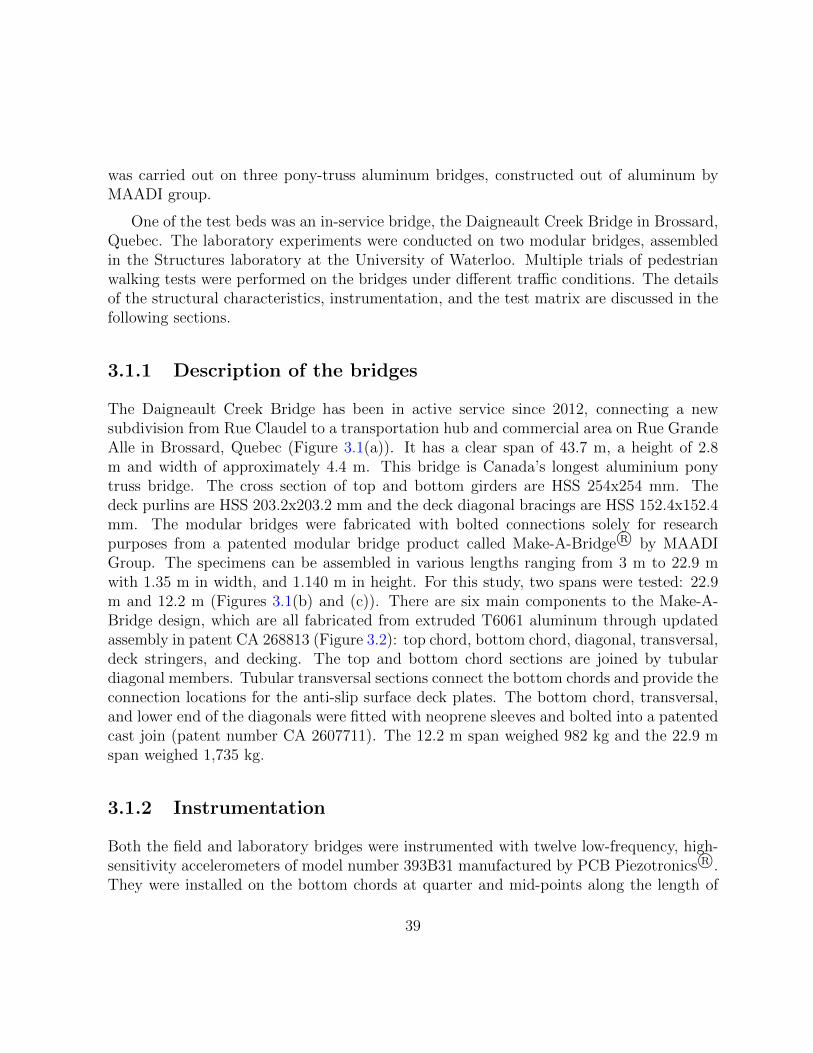
was carried out on three pony-truss aluminum bridges, constructed out of aluminum byMAADI group.

One of the test beds was an in-service bridge, the Daigneault Creek Bridge in Brossard,Quebec. The laboratory experiments were conducted on two modular bridges, assembledin the Structures laboratory at the University of Waterloo. Multiple trials of pedestrianwalking tests were performed on the bridges under different traffic conditions. The detailsof the structural characteristics, instrumentation, and the test matrix are discussed in thefollowing sections.

3.1.1 Description of the bridges

The Daigneault Creek Bridge has been in active service since 2012, connecting a newsubdivision from Rue Claudel to a transportation hub and commercial area on Rue GrandeAlle in Brossard, Quebec (Figure 3.1(a)). It has a clear span of 43.7 m, a height of 2.8m and width of approximately 4.4 m. This bridge is Canada’s longest aluminium ponytruss bridge. The cross section of top and bottom girders are HSS 254x254 mm. Thedeck purlins are HSS 203.2x203.2 mm and the deck diagonal bracings are HSS 152.4x152.4mm. The modular bridges were fabricated with bolted connections solely for researchpurposes from a patented modular bridge product called Make-A-Bridge R© by MAADIGroup. The specimens can be assembled in various lengths ranging from 3 m to 22.9 mwith 1.35 m in width, and 1.140 m in height. For this study, two spans were tested: 22.9m and 12.2 m (Figures 3.1(b) and (c)). There are six main components to the Make-A-Bridge design, which are all fabricated from extruded T6061 aluminum through updatedassembly in patent CA 268813 (Figure 3.2): top chord, bottom chord, diagonal, transversal,deck stringers, and decking. The top and bottom chord sections are joined by tubulardiagonal members. Tubular transversal sections connect the bottom chords and provide theconnection locations for the anti-slip surface deck plates. The bottom chord, transversal,and lower end of the diagonals were fitted with neoprene sleeves and bolted into a patentedcast join (patent number CA 2607711). The 12.2 m span weighed 982 kg and the 22.9 mspan weighed 1,735 kg.

3.1.2 Instrumentation

Both the field and laboratory bridges were instrumented with twelve low-frequency, high-sensitivity accelerometers of model number 393B31 manufactured by PCB Piezotronics R©.They were installed on the bottom chords at quarter and mid-points along the length of

39

Figure 3.1: (a) Daigneault Creek Bridge of span 43.7 m, (b) Modular aluminum bridge ofspan 22.9 m, and (c) Modular aluminum bridge of span 12.2 m

the bridges. The accelerometers were attached to six mounting blocks, three on each sideof the bridges, as shown in Figure 3.3 (a). Each mounting block carried an accelerometerin the lateral and vertical directions (Figure 3.3 (b)). The operable frequency range of theaccelerometer is 0.1 Hz to 200 Hz. The acceleration measurements were acquired usingthree 4-channel A/D data acquisition modules (daisy-chained) of model no. DT9837Amanufactured by Data Translation (Figure 3.3(c)). In addition to the accelerometers,the supports of the modular bridges were instrumented using triaxial load cells of modelno. TR3D-B-4K from Michigan Scientific R© as shown in Figure 3.3(a) and (d). Threestring potentiometers were installed at the mid-span to measure the vertical and lateraldisplacements as shown in Figure 3.3 (a) and (e). The data from the load cells andstring potentiometers (after appropriate signal conditioning) was acquired using a 16-bit12-channel A/D DAQ, model DT9836 also manufactured by DataTranslation.

40

Figure 3.2: Basic assembly of Make-A-Bridge R© specimen

3.1.3 Testing program

Prior to the start of walking tests, the modal characteristics for the bridges were obtainedexperimentally through modal testing. Heel drop tests were conducted on the DaigneaultCreek Bridge in order to estimate its modal properties. Impact loading tests, i.e., hammerdrop were employed on the laboratory bridge specimens for modal identification in thevertical as well as the lateral directions. Impact hammer and pull-then-release tests usinga custom pulley system, were employed on the laboratory bridge specimens for modalidentification in the vertical as well as the lateral directions. The modal properties of thestructures are described in the next section, under dynamic characteristics.

Besides modal testing, a suite of pedestrian tests were conducted on the three bridges.While only individual walking at prescribed rates controlled using a metronome were con-ducted on the field bridge, two people walking synchronously and asynchronously, andcrowds of varying densities in addition to individual walking tests at different walking fre-quencies were performed on the laboratory bridges. All tests consisted of multiple trials inorder to achieve statistical significance. For the Daigneault Creek Bridge, five test subjects(Table 3.1) were involved. With the exception of subject P5, all the test subjects walkedat their normal walking frequencies tabulated in Table 3.1. These frequencies were arrivedat through multiple trials and interviewing test subjects subsequent to the tests regardingtheir perception of the walking rate undertaken. Subject P5 performed 30 trials in ninedifferent frequencies ranging from 1.67 Hz to 2.33 Hz with an interval of 0.083 Hz.

For the laboratory specimens, considerably more repetitions were performed in termsof both inter and intra subject variability. For the 12.2 m bridge, single pedestrian tests

41

Figure 3.3: (a)Plan view of the bridge of length 22.9 m with locations for the instrumen-tation showing (b) accelerometers, (c) vibration data collection system (d) load cells, (e)displacement transducer

were conducted using three male and three female subjects (to minimize gender bias inwalking characteristics). Their weights are listed in Table 3.2. All the tests were repeated30 times for 5 sets of frequencies ranging from 1.67 Hz to 2.33 Hz with an interval of 0.167Hz. Each test subject walked a total distance of 1.83 km during the course of testing. Forthe 22.9 m bridge, seven male and four female subjects participated in the walking tests.Their weights and the number of tests are listed in Table 3.3 for 5 sets of frequencies (1.67Hz to 2.33 Hz with a interval of 0.167 Hz). Each test subject walked a total distance of1.15 km to 3.4 km, depending on the number of trials completed.

Group walking tests on the two laboratory bridges included two people walking syn-chronously and asynchronously, and crowds of varying densities. The test matrices arereported in Tables 3.4 and 3.5 along with the average weights of the pedestrians who par-ticipated in this study. Each set of tests was repeated 30 times for the 12.2 m bridge while10 to 30 trials of tests for each case were performed for the 22.9 m bridge specimen. Crowddensities of 0.2, 0.5, and 1.0 pedestrians per unit of deck area (P/m2) were adopted for thetests on the 12.2 m bridge. However, the 22.9 m bridge specimen was not loaded beyond

42

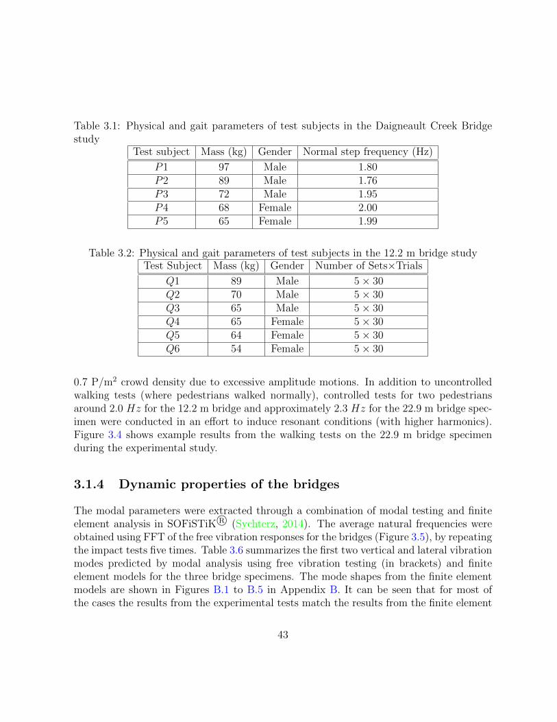
Table 3.1: Physical and gait parameters of test subjects in the Daigneault Creek Bridgestudy

Test subject Mass (kg) Gender Normal step frequency (Hz)

P1 97 Male 1.80P2 89 Male 1.76P3 72 Male 1.95P4 68 Female 2.00P5 65 Female 1.99

Table 3.2: Physical and gait parameters of test subjects in the 12.2 m bridge studyTest Subject Mass (kg) Gender Number of Sets×Trials

Q1 89 Male 5× 30Q2 70 Male 5× 30Q3 65 Male 5× 30Q4 65 Female 5× 30Q5 64 Female 5× 30Q6 54 Female 5× 30

0.7 P/m2 crowd density due to excessive amplitude motions. In addition to uncontrolledwalking tests (where pedestrians walked normally), controlled tests for two pedestriansaround 2.0 Hz for the 12.2 m bridge and approximately 2.3 Hz for the 22.9 m bridge spec-imen were conducted in an effort to induce resonant conditions (with higher harmonics).Figure 3.4 shows example results from the walking tests on the 22.9 m bridge specimenduring the experimental study.

3.1.4 Dynamic properties of the bridges

The modal parameters were extracted through a combination of modal testing and finiteelement analysis in SOFiSTiK R© (Sychterz, 2014). The average natural frequencies wereobtained using FFT of the free vibration responses for the bridges (Figure 3.5), by repeatingthe impact tests five times. Table 3.6 summarizes the first two vertical and lateral vibrationmodes predicted by modal analysis using free vibration testing (in brackets) and finiteelement models for the three bridge specimens. The mode shapes from the finite elementmodels are shown in Figures B.1 to B.5 in Appendix B. It can be seen that for most ofthe cases the results from the experimental tests match the results from the finite element

43

Table 3.3: Physical and gait parameters of test subjects in the 22.9 m bridge studyTest Subject Mass (kg) Gender Number of Sets×Trials

R1 125 Male 5× 30R2 106 Male 5× 10R3 86 Male 5× 10R4 77 Male 5× 10R5 70 Male 5× 30R6 70 Male 5× 30R7 70 Male 5× 10R8 64 Female 5× 15R9 60 Female 5× 10R10 59 Female 5× 10R11 45 Female 5× 30

Table 3.4: Test matrix for 12.2 m pedestrian bridge

TestsWeights of pedestrians (kg)

Mean Standard deviation Maximum MinimumTwo persons 66.5 2.1 68 65

Crowd density of 0.2 P/m2 69 14 89 53Crowd density of 0.5 P/m2 67 9.0 89 60Crowd density of 1.0 P/m2 68 14 90 41

analysis relatively well (see Table 3.6). The differences mainly arise due to the modellingassumptions (e.g. joint fixity) and the contributions to the overall stiffness from the deck,which was not included in the finite element models. For the current study, the first verticaland lateral frequencies from the modal tests are used for all of the bridges, as in all casesthe lower order harmonics of walking only resonate with the fundamental frequency andthe contributions from higher order modes are neglected.

Besides the modal frequencies and mode shapes, the damping ratio is an importantparameter in order to estimate the response of the structure under pedestrian loading. Forthe 12.2 m and 22.9 m laboratory specimens, damping is estimated from impact tests usingthe simple free decay method (Humar, 2012) for the first vertical and lateral modes, as onlythese modes are important from a serviceability assessment standpoint. The details of themethods to estimate damping ratio are presented in Appendix C. The average dampingratios estimated for the bridge specimens are listed in Table 3.7. For the current analysis

44

Table 3.5: Test matrix for 22.9 m pedestrian bridge

TestsWeights of pedestrians (kg)

Mean Standard deviation Maximum MinimumTwo persons 67.5 3.5 70 65Four persons 65 4.1 70 60

Crowd density of 0.2 P/m2 72 7.5 82 65Crowd density of 0.3 P/m2 70 11.8 82 45Crowd density of 0.5 P/m2 71 10.8 82 45Crowd density of 0.7 P/m2 68 12.4 100 45

half of the total mass is assumed to participate in the first modes of vibration.

Table 3.6: Natural frequencies and mode shapes for the bridges through finite elementanalysis and modal testing

Daigneault Creek Bridge 12.2 m Bridge 22.9 m Bridge

fn(Hz) Mode Shape fn(Hz) Mode Shape fn(Hz) Mode Shape3.34(3.43) Vertical 2.3(2.3) Lateral 1.0(1.29) Lateral6.8(6.9) Lateral 6.1(4.9) Lateral 2.6(2.3) Lateral9.5(9.4) Lateral 13.0(11.8) Vertical 4.4(4.58) Vertical

10.9(10.3) Vertical 35.1(32.6) Vertical 14.7(12.8) Vertical

*Note: FE result is given along with result based on modal testing in brackets ()

Table 3.7: Damping ratio for the bridges through modal testingBridge Vertical LateralDaigneault Creek bridge 0.01 0.0122.9 m lab specimen 0.008 0.03312.2 m lab specimen 0.012 0.030

3.2 Performance of design guidelines

All of the design guidelines reviewed in the current study adopt a two-step approachas discussed in Section 2.2. When structural frequency is within the critical frequency

45

Figure 3.4: (a) One pedestrian and (b) groups of pedestrians walking on the 22.9 m bridgespecimen during the experimental study carried out in the Structures Laboratory at theUniversity of Waterloo

0 2 4 6 8 10 12

-0.5

0

0.5

0 10 20 30 40 500

0.01

0.02

0 2 4 6 8 10 12Time (Sec)

-0.5

0

0.5

Acc

eler

atio

n (m

/s2 )

0 10 20 30 40 50Frequency (Hz)

0

0.005

0.01

0.015

Four

ier

ampl

itude

(b)(a)

(c)

4.60

4.60

23.24

12.70

(d)

Figure 3.5: Acceleration time history ((a) and (c)) and corresponding Fourier spectrum((b) and (d)) of impact testing at centre ((a) and (b)) and quarter (((c) and (d))) spansof the 22.9 m bridge specimen

46

ranges in Table 2.3, dynamic analysis is required to assess the serviceability of the bridges.Despite different functional forms used by these guidelines, the dynamic analysis is basedon a common underlying idea that estimates of the response under N pedestrians (aN) isobtained by multiplying the response due to a single pedestrian (as) with a multiplicationfactor (SN):

aN = SN × as (3.1)

The multiplication factors SN are summarized in Table 3.8. All the parameters in Table3.8 are already defined in Section 2.2.

The structural response due to a single pedestrian as, is estimated from a movingconcentrated force (Pmov) or a uniformly distributed force p(x), which can be equivalentlyrepresented as a concentrated load of p(x)L. The periodic walking load is represented usingEquation 2.1. The DLFs prescribed by the guidelines are summarized in Table 3.9. In thissection, performance of the four guidelines, ISO 10137, Eurocode 5, British National Annexto Eurocode 1, and SETRA, are evaluated. First, this periodic load model is validatedunder single pedestrian walking trials employing the DLF values from Table 3.9. Next, theperformance of the design methodologies are assessed in terms of serviceability assessmentof the bridges as well as response predictions under groups of walking pedestrians.

Table 3.8: Multiplication factors for crowd loading used by existing guidelinesCodes Vertical Lateral

ISO 10137√N

√N

Eurocode 5 0.23kvertN 0.18khorN

British National Annex k(fv)√

1 + γ(N − 1) (Group) –

or 1.8k(fv)√

γNλ

(Crowd) –

SETRA 10.8√ζnNψv for d < 1.0 10.8

√ζnNψl for d < 1.0

1.85√Nψv for d ≥ 1.0 1.85

√Nψl for d ≥ 1.0

3.2.1 Single pedestrian load model

Response simulation

This section focuses on evaluating the moving periodic models for single pedestrian walkingon PBs. The performance study is restricted only to vertical vibration of the PBs andconsiders both resonant and non-resonant scenarios. In order to simplify the analytical

47

determination of the response, the pedestrian is assumed to walk on the structure at auniform walking speed. Moreover, the structure is assumed to be linearly elastic. Hence,the modal equation of motion for the bridge response in Equation 2.24 corresponding tomode of vibration under consideration is employed. For the present study, the analyticalsolution, derived in Appendix A, based on the works by Abu-Hilal and Mohsen (2000) andHilal and Zibdeh (2000), is adopted through employing the principle of superposition ofresponses from a constant moving load G and the harmonic loading terms Gαm sin(m2πfs)for mth harmonic in Equation 2.24:

Yn = Xn +m∑i=1

Xmn (3.2)

where Xn and Xmn are the displacement response of the simply supported beam in Figure2.12 under respectively constant and harmonic moving loads as derived in Appendix A. Theacceleration response history Yn is then estimated by employing a second order derivationon Yn.

Table 3.9: Dynamic load factors adopted by guidelines and standardsCodes vertical LateralISO 10137 α1 = 0.37fs − 1.0 α1 = 0.10

α2 = 0.1α3 = α4 = α5 = 0.06

Eurocode 5 α1 = 0.4 α1 = 0.1α2 = 0.2

British Annex to Eurocode 1 α1 = 0.4 −−−α2 = 0.14∗

α3 = 0.051∗

SETRA α1 = 0.4 α1 = 0.05α2 = 0.1 α2 = 0.01

*Note: The DLF values are corresponding to k′(fv)

Response data processing

In order to evaluate the performance of the design walking load models in predicting theresponse of the PBs, only the modal response corresponding to the first mode of vibrationof the bridge is considered. The measurements were first truncated to the forced vibration

48

phase only, and then low-pass filtered (with a cut-off frequency of 10 Hz in the caseof the Daigneault Creek bridge and 15 Hz in the case of laboratory bridge specimens)in order to filter out the contributions of second and higher modes of vibrations. Thenthe measured and simulated acceleration time histories were converted to the frequencydomain through Fourier transform (FFT). Figures 3.6 to 3.9 show the comparison of theacceleration time histories and corresponding Fourier spectra of the time histories at thecentre of the Daigneault Creek Bridge for non-resonant (2 Hz) and near-resonant (1.75Hz) conditions.

It can be seen from Figure 3.6 that the predictions overestimate the measurements bothin terms of maximum and root mean square of acceleration. Furthermore, the guidelinesare not consistent due to the different number of harmonics taken into consideration, aswell as the different DLF values used. The Fourier spectra in Figure 3.7 show that thesimulated response from the design models only contains contributions from the walkingharmonics with negligible contributions from the transients (natural frequency of the struc-ture). However, the response measurements contain contributions from both the transientand the excitation harmonics. In order to simulate the bridge responses, the walking loadis assumed to be moving over the entire span of the bridge at constant speed and thetransient part of the total response has sufficient time to decay, which leads to negligi-ble contributions from the transients in the predicted response. But, in reality, the heelimpacts the ground at the beginning of every step, leading to insufficient time to decayof the transients and hence significant contributions from the transients in the measuredresponse. It is certain that the Fourier spectra are dominated by the resonating harmonic(second) for the near-resonant case, and the frequency characteristics of the predicted re-sponse by the design models in such cases agrees with the measurements. However, all themodels overestimate the measurements in near-resonant conditions (Figure 3.8), which isexpected for conservative design.

It is clear that application of the periodic load model results in the excitation harmon-ics (steady-state solution) dominating the response, with negligible contributions from thetransient response. However, in all the three bridges tested in this study, it was observedthat the transients are of the same order of magnitude or sometimes larger than the steady-state components. Since the bridges tested here were non-resonant (in their fundamentalmode) with the the excitation frequency, a significant portion of the response must havebeen contributed by the transients. Hence, the response data was filtered to separate thecontributions from various frequency components in the spectra after truncating to theforced vibration phase only, and then low-pass filtered, as discussed before. In order toenable a comparison between the simulated and measured responses, individual contribu-tions from the harmonics (both natural frequency as well as excitation) are extracted from

49

the total response. For this purpose, the filtered response signal is assumed to contain afinite number of damped sinusoids and the modified Prony method based on total leastsquares approach (known as TLS-Prony) (Rahman and Yu, 1987) is used to estimate themagnitude, frequency, phase, and damping of the individual sinusoids. This method ismore robust with respect to measurement noise as compared to the native form of theProny’s method (Hildebrand, 1956), and allows a better approximation of the responseusing damped sinusoids compared to the basic FFT approximation. The basic idea of theTLS-Prony method (Hildebrand, 1956; Rahman and Yu, 1987) is discussed in the followingparagraph.

Assume that x[n] is a sampled version of a equally-spaced time-series (e.g. acceleration).The Prony approximation consisting of M damped harmonics can be written as Hildebrand(1956):

y[n] =M∑k=1

hkznk (3.3)

where, hk = Akejψk and zk = e(αk+j2πfk)Ts . Ts is the sample time, fk is the frequency in

cycles per second, ψk is the phase of the kth component, and αk is the damping coefficientof the kth component. The M -length vector A represents the amplitude of the dampedsinusoids, yielding kth contributions from the excitation and transient harmonics in themeasured signals. These amplitudes directly yield the contributions from the harmonics ofinterest. The key steps in estimating these coefficients along with the frequencies, phaseand damping coefficients are summarized in Appendix D.

As mentioned earlier, none of the three specimens are resonant in their lowest verticalmode with the first harmonic of pedestrian pacing frequency. However, they are in res-onance, or nearly resonant, with the higher harmonics of the excitation frequency. TheDaigneault Creek Bridge is nearly resonant (3.43 Hz) with the second harmonic of thewalking frequency at 1.67 Hz and 1.75 Hz (slow walking), while the fundamental fre-quency of the 12.2 m bridge specimen (11.81 Hz) is close to resonance with the sixthand fifth harmonics of 2 Hz and 2.33 Hz walking frequencies, respectively. Similarly, thenatural frequency of the 22.9 m bridge specimen (4.58 Hz) is close to the second harmonicof the walking frequency at 2.33 Hz (fast walking). While all three bridges would be con-sidered as being relatively insensitive to pedestrian forces from a vertical flexural responsestandpoint, the peak vertical acceleration responses at the centre recorded during singlepedestrian tests reached 0.5, 1.2, and 3.6 m/s2 for the three bridges respectively (maximumfor all tests conducted).

50

0 10 20 30-0.1

0

0.1

Acc

eler

atio

n (m

/s2 ) ISO 10137

0 10 20 30-0.1

0

0.1Eurocode 5

0 10 20 30Time (Sec)

-0.1

0

0.1

Acc

eler

atio

n (m

/s2 ) British National Annex

0 10 20 30Time (Sec)

-0.1

0

0.1SÉTRA

0 10 20 30Time (Sec)

-0.05

0

0.05

Acc

eler

atio

n (m

/s2 )

Field measurement

(a) (b)

(c) (d)

(e)

M:0.039

R:0.024

R:0.009

M:0.055 M: 0.045

R:0.018

R:0.018

M:0.093

R:0.040

M:0.033

Figure 3.6: The acceleration time history at the centre of the Daigneault Creek Bridge forwalking at 2.0 Hz in the case of simulated response using (a) ISO 10137, (b) Eurocode 5,(c) British National Annex, and (d) SETRA models and (e) field measurements (Here, Mare R represents respectively the maximum and RMS accelerations)

51

0 2 4 6 80

0.02

0.04

Four

ier

ampl

itude

ISO 10137

0 2 4 6 80

0.02

0.04

Eurocode 5

0 2 4 6 8Frequency (Hz)

0

0.02

0.04

Four

ier

ampl

itude

British National Annex


0

0.02

0.04

SÉTRA


0

0.005

0.01

Four

ier

ampl

itude

Field measurement

Firstharmonic

SecondharmonicTransient First

harmonic

Transient Secondharmonic

Transient TransientSecondharmonicFirst

harmonicFirstharmonic

Secondharmonic

(d)

(e)

(b)(a)

Firstharmonic

Transient

Secondharmonic

(c)

Figure 3.7: Fourier spectra of the acceleration response at the centre of the DaigneaultCreek Bridge for walking at 2.0 Hz in the case of simulated response using (a) ISO 10137,(b) Eurocode 5, (c) British National Annex, and (d) SETRA models and (e) field mea-surements

52

0 10 20 30 40-0.5

0

0.5

Acc

eler

atio

n (m

/s2 ) ISO 10137

0 10 20 30 40-0.5

0

0.5Eurocode 5

0 10 20 30 40Time (Sec)

-0.5

0

0.5

Acc

eler

atio

n (m

/s2 ) British National Annex

0 10 20 30 40Time (Sec)

-0.5

0

0.5SÉTRA

0 10 20 30 40Time (Sec)

-0.1

0

0.1

Acc

eler

atio

n (m

/s2 ) Field measurement

(a) (b)

(c) (d)

(e)

M:0.065

M:0.199

M:0.268 M:0.193

R:0.022

R:0.092

R:0.129 R:0.092

R:0.231

M:0.469

Figure 3.8: The acceleration time history at the centre of the Daigneault Creek Bridge forwalking at 1.75 Hz in the case of simulated response using (a) ISO 10137, (b) Eurocode5, (c) British National Annex, and (d) SETRA models and (e) field measurements (Here,M are R represents respectively the maximum and RMS accelerations)

53

0 5 100

0.05

0.1

0.15

Four

ier

ampl

itude

ISO 10137

0 5 100

0.1

0.2

0.3Eurocode 5

0 5 10Frequency (Hz)

0

0.1

0.2

Four

ier

ampl

itude



0

0.05

0.1

0.15SÉTRA


0

0.01

0.02

0.03

Four

ier

ampl

itude

Field measurement

(a) (b)

(c) (d)

(e)

Firstharmonic

Firstharmonic

Near-resonance

Near-resonanceNear-resonance

Firstharmonic

Firstharmonic

Near-resonance

Firstharmonic

Near-resonance

Figure 3.9: Fourier spectra of the acceleration response at the centre of the DaigneaultCreek Bridge for walking at 1.75 Hz in the case of simulated response using (a) ISO10137, (b) Eurocode 5, (c) British National Annex, and (d) SETRA models and (e) fieldmeasurements

54

Results from the Daigneault Creek Bridge

As described earlier, five test subjects walked naturally on the Daigneault Creek Bridge andtheir normal step frequencies are listed in Table 3.1. Moreover, test subject P5 walked atnine discrete frequencies ranging from 1.67 Hz to 2.33 Hz. 30 trials were conducted at eachpacing frequency to ensure statistical significance. The mid-span vertical response of thebridge is simulated using the DLF values proposed by the design guidelines. Due to the nearresonant condition with the second harmonic of the walking frequencies at 1.67 and 1.75Hz, the contributions from the first two harmonics of the load along with the fundamentalfrequency of the bridge (3.43 Hz) are of interest. The amplitudes corresponding to thesefrequencies are estimated from the measured and simulated acceleration data using theTLS-Prony method.

Figure 3.10 compares the measured and simulated amplitudes corresponding to thefrequencies of interest, i.e., the first two harmonics of the walking frequency and funda-mental frequency, for the five test subjects walking at their normal walking frequency. Theestimated amplitudes for the simulated and measured responses are normalized with therespective weight of the test subjects. It can be observed that the design models overesti-mate the measured response corresponding to the first two harmonics with relatively largedeviations for subjects P1 and P2 for the second harmonic of walking frequency (Figure3.10(b)), which produced near-resonant conditions from the second harmonic. Further-more, the models significantly underestimate the contribution to the response from thenatural frequency of the structure (Figure 3.10 (c)) and this trend has higher deviation forthe non-resonant compared to the near-resonant cases.

Figure 3.11 shows the results of intra-subject variability for test subject P5 at differentwalking frequencies (1.67 Hz to 2.33 Hz), creating near-resonant conditions with the sec-ond harmonic of 1.67-1.75 Hz. Comparison of the amplitudes shows that the design modelssignificantly overestimate the measured response contributions (Figures 3.11 (a) and (b))from the first and second harmonics. The deviation corresponding to the second resonat-ing harmonic (1.67-1.75 Hz) is larger, which was observed as well previously. However,both models are unable to capture the contribution from transients for the non-resonatingwalking frequencies (1.8-2.4 Hz) to the response (Figure 3.11 (c)). In these cases, thereis significant natural frequency contribution to the overall response, which is not capturedby the load models. So, an important observation is that the models, while conservativefor the resonant region (in this case where the second harmonic matches the first flexuralmode), tend to be unconservative in the non-resonant range.

In comparing the simulated amplitudes by all the design models, it is certain that all ofthe provisions are inconsistent with each other due to different values of DLF with those

55

by Eurocode 5 being overly conservative.

P1 P2 P3 P4 P5Test subjects

0

0.5

1

1.5

2

Am

plitu

de/m

ass

(m/s2 /k

g) ×10-4


0

1

2

3

4×10-3


0

0.5

1

1.5

2

Am

plitu

de/m

ass

(m/s2 /k

g) ×10-3

Field measurementISO 10137Eurocode 5British NationalAnnexSÉTRA

(c)

(b)(a)

Figure 3.10: Comparison of simulated and measured amplitudes corresponding to: (a) thefirst harmonic, (b) the second harmonic, and (c) the fundamental frequency, in the case ofDaigneault Creek Bridge

Results from the 12.2 m bridge specimen

For the 12.2 m bridge specimen, both inter- and intra-subject variabilities were consideredusing several trials with six test subjects (Table 3.2) at five sets of frequencies, 30 timeseach. A total of 900 records were processed considering both inter- and intra-subjectvariabilities. In this case, there is a possibility of near resonant condition with the fifthand sixth harmonics at 2.33 Hz and 2.0 Hz walking frequencies. Hence, the contributionsto the total response from the first, fifth, and sixth harmonics of the excitation frequenciestogether with the fundamental frequency of the bridge (11.81 Hz) are considered. Byapplying the TLS-prony method on the simulated and measured acceleration data, theamplitudes corresponding to these frequencies of interest are extracted from the total

56

1.6 1.8 2 2.2 2.4Step frequency (Hz)

0

0.005

0.01

0.015

0.02A

mpl

itude

(m/s2 )

ExperimentalISO 10137Eurocode 5British NationalAnnexSÉTRA


0

0.05

0.1

0.15

0.2


0

0.05

0.1

0.15

0.2

Am

plitu

de(m

/s2 )

(a) (b)

(c)

Figure 3.11: Statistical results for simulated and measured amplitudes corresponding toP5 for: (a) the first harmonic, (b) the second harmonic, and (c) the natural frequenciesfor the Daigneault Creek Bridge

response data series. The extracted amplitudes are normalized by the weight of each testsubject and compared in Figure 3.12. Error bars from several trials are also plotted torepresent both inter- and intra-subject variabilities.

Similar to the observations from the Daigneault Creek Bridge, all the design load modelslead to a response that is dominated by the forcing frequency, with little contributionfrom the transients. Below 2 Hz, the model predictions and experimental results for thefirst harmonic follow closely because the DLFs used in the load models were developedfor rigid surfaces, which in this case closely resemble a rigid structure with little or nopedestrian-structure interaction. However, for excitation frequencies where there is near-resonance in the higher harmonics (fs between 2.0 and 2.33 Hz), the models significantlyunderestimate the acceleration response levels (Figure 3.12 (a)). It is noteworthy that onlyISO 10137 includes five harmonics. Thus, other guidelines except ISO 10137 fail to estimatethe response contributions from the fifth harmonic, which is near resonance at 2.33 Hz(Figure 3.12 (b)). Also none of the guidelines consider the contributions from the sixth

57

1.6 1.8 2 2.2 2.40

0.5

1

1.5

Am

plitu

de/m

ass(

m/s

2 /kg) ×10-3

ExperimentalISO 10137Eurocode 5British NationalAnnexSETRA

1.6 1.8 2 2.2 2.40

0.005

0.01

0.015

0.02


0

2

4

6

8

Am

plitu

de/m

ass(

m/s

2 /kg) ×10-3


0

0.005

0.01

0.015

0.02(a)

(d)(c)

(b)

Figure 3.12: Comparison of contributions for simulated and measured amplitudes fromthe: (a) first harmonic (b) fifth harmonic, (c) sixth harmonic, and (d) natural frequencyin the case of the 12.2 m bridge specimen

harmonic, which is near resonant with 2 Hz resulting in a significant contribution in themeasured response (Figure 3.12 (b)). Moreover, the natural frequency contributions aresignificant in the measurements (Figure 3.12(d)) while all the design models lead to verylittle or negligible contributions at the natural frequency for non-resonating frequencies(1.6-2.0 Hz). It is also seen from Figure 3.12 (b) that there is significant natural frequencycontributions in the design model for ISO 10137 for fs between 2.1-2.33 Hz due to thenear resonance condition with the fifth harmonic of walking.

Results from the 22.9 m bridge specimen

For the 22.9 m bridge specimen, eleven test subjects participated in the walking tests(Table 3.3). All of the test subjects were asked to walk at five sets of frequencies, 10-30 times each, as mentioned in the previous section. A total of 975 data series wererecorded during this experimental study to cover inter- and intra-subject variabilities. As

58

the second harmonic for 2.17 Hz and 2.33 Hz walking frequencies are near the naturalfrequency of the structure (4.58 Hz), the amplitudes corresponding to the first and secondharmonics of walking along with the fundamental frequency of the bridge are estimatedfrom the measured and simulated acceleration data series through the TLS-Prony method.Moreover, the third harmonic contribution is also shown as an example of a case where thestructure is not in resonance with the walking frequency or its harmonics.

As before, all the extracted measured and simulated amplitudes are normalized withrespect to the weight of test subjects. Error bar plots of the measured amplitudes arecompared with the simulated results in Figure 3.13. The structure is in a near resonantcondition with the second harmonic of the faster walking rates. On the other hand, thestructure behaves rigidly with respect to the pedestrian excitation for slower walking fre-quencies and hence the model predictions are near experimental observations. As the speedof walking increases, the walking harmonic becomes close to the structural frequency andthus, the structure exhibits pedestrian-structure interaction leading to a lower estimationof response contributions from the first two harmonics. This behaviour is also evidentin the third harmonic using the British National Annex and ISO 10137, which includeupto three harmonics in their predictions. On the other hand, Eurocode 5 overestimatescontributions from the second harmonic as the corresponding DLF is almost twice com-pared to other guidelines. Similar to other cases, the simulated response shows very littlecontribution from the natural frequency component for the non-resonant condition.

59

1.6 1.8 2 2.2 2.40

1

2

3

Am

plitu

de/m

ass

(m/s2 /k

g) ×10-3

ExperimentalISO 10137Eurocode 5British NationalAnnexSÉTRA

1.6 1.8 2 2.2 2.40

0.01

0.02

0.03


0

1

2

3

Am

plitu

de/m

ass

(m/s2 /k

g) ×10-3


0

0.01

0.02

0.03

(b)(a)

(c) (d)

Figure 3.13: Simulated and measured amplitude contributions corresponding to the: (a)first harmonic, (b) second harmonic, (c) third harmonic, and (d) natural frequencies forthe 22.9 m bridge specimen

Summary of key findings from single pedestrian studies

Three are three broad findings from a comparison study involving predicted and measuredresponses under single pedestrian walking:

1. The periodic load models adopted by the guidelines and standards fail to estimatethe transient contributions (i.e. at the natural frequency of the structure) for non-resonating cases, while they significantly over-estimate the forced response for theresonant cases.

2. For the case of resonance with a higher harmonic, the contribution from the corre-sponding non-resonating harmonics are underestimated by the models, which maybe due to pedestrian-structure interaction.

3. For a fully non-resonant case (i.e. none of the harmonics are in resonance with theexcitation), the models estimate the observations relatively well.

60

These issues become very important for lightweight structures such as aluminum bridges,which tend to exhibit natural frequencies outside what is typically considered as designfrequency ranges, however tend to be lively due to their low inherent damping and lightweight. Hence, more sophisticated models that address these shortcomings are needed tobetter estimate serviceability in such cases.

3.2.2 Serviceability assessment under groups of pedestrians

Response estimation under a crowd is obtained by first estimating the response due to asingle pedestrian and then multiplying it with a factor specified by the guidelines. As-suming that the bridges can be modelled as a simply supported beam where only onemode of vibration dominates, the maximum ith mode resonant acceleration under a singlepedestrian load can be estimated using the following equation:

as,i =PiMi

1

2ζi(3.4)

where, Pi, Mi and ζi are the generalized (modal) load, mass, and damping ratio of thestructure. For an uniformly distributed load p(x), the generalized load is given by 2

πp(x)L

for the first mode of vibration and half of this value for the second mode of vibration.Similarly, the generalized load for a moving load Pmov for any mode is 2

πPmov. By replacing

the modal load, the maximum acceleration under N pedestrians can be estimated fromEquations 3.1 and 3.4 (removing the subscript i):

aN =SNGnαmnπMnζn

(3.5)

where, n represents the characteristic value of the parameter suggested by the guidelines.The serviceability of the bridge is assessed through satisfying the following equation:

aln ≥ aN (3.6)

None of the guidelines listed in Table 2.3 suggest performing a dynamic analysis forthe 12.2 m bridge specimen in the vertical direction, with a frequency of 11.81 Hz, whileits lateral frequency (2.30 Hz) falls within the critical range proposed by Eurocode 5 andSETRA, and thus a dynamic analysis is required. Similarly, all the guidelines recommend adynamic analysis in the vertical (4.58 Hz) and the lateral (1.29 Hz) directions for the 22.9m bridge. The maximum accelerations are estimated from either the formulae available in

61

the guidelines, or through Equation 3.5 if a suitable formulae is not available, followed bya serviceability assessment using Equation 3.6.

Figures 3.14 (a) to (c) show results from measurements for the 12.2 m bridge in thevertical direction for a density of 1.0 P/m2. It is evident from Figures 3.14 (b) to (c) thatthere is a local concentration of vibration energy in the spectrogram around the 12 Hzrange. This observation points towards near-resonant conditions prevailing with a higherharmonic of the walking frequency approaching the structural frequency in the 11.5-13.0Hz range. A similar energy concentration is found in the measurements under other crowddensities (not shown here), while the spectral region containing the peak magnitudes be-come more concentrated with a decrease in the crowd density. Figures 3.14 (d)-(f) showthe measurement results for the same bridge in the lateral direction. Unlike the verticaldirection, lateral measurements show a more broad-band response with comparable re-sponse contributions from harmonics of the excitation frequency as well as the structuralfrequency, which is clearly a non-resonant case. As shown in the Figures 3.14 (e) and(f), 0.83 Hz and 2.67 Hz are respectively the first and third harmonics of the walkingfrequencies in the lateral direction, while 2.3 Hz is the structural frequency. Resonanceconditions are difficult to achieve as it requires walking speeds that are unrealistic, espe-cially in pedestrian groups. It is interesting to observe that the design provisions assumethis bridge to be in resonance with the second harmonic of lateral walking frequency, whichwill result in overly conservative estimates of the design accelerations.

Similar to the 12.2 m bridge specimen, Figures 3.15 (a) and (f) are plotted for the 22.9m bridge specimen for a density of 0.7 P/m2. The spectrogram and the Fourier spectrumrespectively in Figures 3.15 (b) and (c) show that the response of the bridge is non-resonantin the vertical direction. Resonance conditions are unlikely to occur as it requires walkingfrequency of the group to be near 2.3 Hz, which is difficult to achieve for this pedestriandensity (Butz et al., 2008). Lateral synchronization around 1 Hz is also observed in Figures3.15 (d)-(f). Groups of pedestrians drive the structural frequency (1.29 Hz) down to 1 Hz,which leads to a near resonance condition with the walking frequency.

62

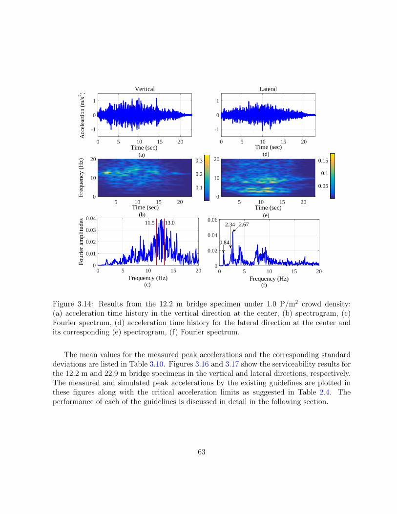
0 5 10 15 20Time (sec)

-1

0

1

Acc

elea

rtio

n (m

/s2 )

Vertical

0 5 10 15 20Time (sec)

-1

0

1

Lateral

5 10 15 20Time (sec)

0

10

20

Freq

uenc

y (H

z)

0.1

0.2

0.3

5 10 15 20Time (sec)

0

10

20

0.05

0.1

0.15


0

0.01

0.02

0.03

0.04

Four

ier

ampl

itude

s


0

0.02

0.04

0.06

(d)(a)

(c)

(b)

0.84

2.34 2.6713.011.5

(f)

(e)

Figure 3.14: Results from the 12.2 m bridge specimen under 1.0 P/m2 crowd density:(a) acceleration time history in the vertical direction at the center, (b) spectrogram, (c)Fourier spectrum, (d) acceleration time history for the lateral direction at the center andits corresponding (e) spectrogram, (f) Fourier spectrum.

The mean values for the measured peak accelerations and the corresponding standarddeviations are listed in Table 3.10. Figures 3.16 and 3.17 show the serviceability results forthe 12.2 m and 22.9 m bridge specimens in the vertical and lateral directions, respectively.The measured and simulated peak accelerations by the existing guidelines are plotted inthese figures along with the critical acceleration limits as suggested in Table 2.4. Theperformance of each of the guidelines is discussed in detail in the following section.

63

0 10 20 30Time (sec)

-2

0

2

Acc

eler

atio

n (m

/s2 ) Vertical

0 10 20 30Time (sec)

-2

0

2

Lateral

5 10 15 20 25 30Time (sec)

0

5

10

15

Freq

uenc

y (H

z)

0.10.20.30.40.5

5 10 15 20 25 30Time (sec)

0

5

10

15

0.2

0.4

0.6

0.8

1

0 5 10 15Frequency (Hz)

0

0.05

0.1

Four

ier

ampl

itude

s

0 5 10 15Frequency (Hz)

0

0.1

0.2(b)

(c)

(e)

(a)

1.94

4.0

0.97

(d)

(f)

Figure 3.15: Results from the 22.9 m bridge specimen under 0.7 P/m2 crowd density:(a) acceleration time history in the vertical direction at the center, (b) spectrogram, (c)Fourier spectrum, (d) acceleration time history for the lateral direction at the center andits corresponding (e) spectrogram, (f) Fourier spectrum.

64

Table 3.10: Mean and standard deviation for the experimental peak accelerations on the12.2. and 22.9 m bridge specimens

Bridge Length Walking TestsPeak Acceleration in m/s2

Vertical Direction Lateral Direction

MeanStandardDeviation

MeanStandardDeviation

12.2 m

2 Pedestrians (Synchronous) 1.170 0.250 0.233 0.0332 Pedestrians (Asynchronous) 1.132 0.183 0.232 0.0290.2 Pedestrians/m2 0.798 0.199 0.476 0.1080.5 Pedestrians/m2 0.936 0.146 0.622 0.0971.0 Pedestrians/m2 0.951 0.168 0.800 0.159

22.9 m

2 Pedestrians (Synchronous) 1.750 0.451 2.100 0.3082 Pedestrians (Asynchronous) 1.486 0.239 1.853 0.5644 Pedestrians 1.584 0.547 1.640 0.2860.2 Pedestrians/m2 1.092 0.170 1.503 0.3240.3 Pedestrians/m2 1.285 0.232 1.015 0.3010.5 Pedestrians/m2 1.285 0.285 0.675 0.2480.7 Pedestrians/m2 1.442 0.178 0.679 0.250

ISO 10137

ISO 10137 does not specify critical frequency limits directly and a dynamic response anal-ysis is needed using the harmonic load model in Equation 2.6. However, it implicitlysuggests dynamic analysis for the vertical and lateral frequencies up to 12 Hz and 1.2 Hz,respectively. Hence these values can be taken as the limits for frequency evaluation of thestructures. In the vertical direction, both the structures are subjected to dynamic analysisas their frequencies are below 12 Hz, while no analysis is required in the lateral direction.Furthermore, this guideline uses root mean square (RMS) values for serviceability checks(Figure 2.8) instead of peak values, which are provided as a function of frequency. For com-parison purposes with other guidelines, the current study adopts peak acceleration as theevaluation parameter in lieu of RMS acceleration. The RMS values for the limit accelera-tion in Figure 2.8 are converted to peak values by multiplying with a

√2 factor (Zivanovic

et al., 2005), while the peak values for the predicted and experimental accelerations areestimated directly without scaling.

Dynamic load factor coefficients are provided in Table 2.5 for the five harmonics inthe vertical direction. As discussed before, either a full dynamic analysis including all the

65

harmonics or the resonant SDOF approach can be employed here for response estimation.Including all the harmonics in the calculations results in higher estimates for the responseas compared to the resonant SDOF approach, which includes only the resonating harmonic.Results from both of these approaches (Equation 3.5 and the procedure described in Section3.2.1) revealed that the difference between the two approaches is small, with deviations inthe range of 4% to 12% under all crowd sizes. Hence, due to its simplicity, the resonantSDOF approach is adopted for further analysis.

0

1

2

3

4

5

6

7

8

9

Pea

k ac

cele

ratio

n(m

/s2 )

Measurement

ISO 10137

Eurocode 5


SÉTRA (Limit I)

SÉTRA (Limit II)

SÉTRA (Limit III)

ISO 10137

0

2

4

6

8

10

12

14

16Measurement

Eurocode 5


SÉTRA(unloaded)

SÉTRA (loaded)

ISO 10137

Eurocode 5


SÉTRA (Limit I)

SÉTRA (Limit II)

SÉTRA (Limit III)

ISO 10137

(a) (b)

2P 2P 4P 0.2 0.3 0.5 0.7

Sync Async P/m2 P/m2 P/m2 P/m2 2P 2P 0.2 0.5 1.0

Sync Async P/m2 P/m2 P/m2

Figure 3.16: Comparison of measured and predicted peak accelerations along with thecomfort limits as proposed by guidelines in the vertical direction for the (a) 12.2 m and(b) 22.9 m bridge (P stands for pedestrians; Limit I, Limit II and Limit III by SETRAguideline are defined in Table 2.4)

The specified acceleration limit in the vertical direction is 0.63 m/s2 for the 12.2 mbridge specimen after converting the RMS acceleration to peak from Figure 2.8. As shownin Figure 3.16(a), both the measured and predicted maximum accelerations do not satisfythe specified limit for this bridge. Since no guidance is provided regarding the reduction of

66

walking speed as a function of the pedestrian density in this guideline, the fifth harmonic ofpedestrian walking at 2.3 Hz is assumed to be in resonance with the first vertical frequencyof the unloaded bridge (11.81 Hz). This leads to an overestimation of the predictedresponses and the deviation increases with an increase in the crowd density (+156 % to+829 %). This increase in the deviation can be explained by a reduction in the effectivewalking frequency of the group of pedestrians with increasing density and a simultaneousreduction in the natural frequency due to the pedestrian added mass. Furthermore, thelarger magnitude of the load factors αm compared to the values provided in the recentliterature (Brownjohn et al., 2004b) also contribute to this overestimation.

0

0.2

0.4

0.6

0.8

1

1.2

Pea

k A

ccel

erat

ion

(m/s2 )

MeasurementEurocode 5SÉTRA (unloaded)SÉTRA (loaded)ISO 10137Eurocode 5SÉTRA (Limit I)SÉTRA(Limit II)SÉTRA (Limit III)

0

0.5

1

1.5

2

2.5

3

3.5

MeasurementEurocode 5SÉTRA (unloaded)SÉTRA (loaded)ISO 10137Eurocode 5SÉTRA (Limit I)SÉTRA(Limit II)SÉTRA (Limit III)

(a) (b)

2P 2P 0.2 0.5 1.0


2P 2P 4P 0.2 0.3 0.5 0.7

Sync Async P/m2 P/m2 P/m2 P/m2

Figure 3.17: Comparison of measured and predicted peak accelerations along with thecomfort limits as proposed by guidelines in the lateral direction for the (a) 12.2 m and(b) 22.9 m bridge (P stands for pedestrians; Limit I, Limit II and Limit III by SETRAguideline are defined in Table 2.4)

67

Similar characteristics are observed for the vertical mode of the 22.9 m bridge at 4.58Hz, (Figure 3.16(b)). The vertical acceleration limit for this bridge is 0.42 m/s2. Thisbridge does not satisfy the serviceability criterion, both as measured and as predicted.Furthermore, the guideline assumes a second harmonic of fast walking frequency resonatingwith the structural frequency. As with the 12.2 m bridge, the discrepancy between themeasured and predicted peak accelerations increases with an increase in the crowd density(+198 % to +768 %). While near resonant condition with the second harmonic is observedfor sparse density (two pedestrian cases) in the measured data, this does not occur as thedensity increases (at or beyond 0.7 P/m2).

The lateral frequencies for both the 12.2 m and the 22.9 bridge specimens (2.3 Hz and1.29 Hz, respectively) are outside the range of the first harmonic of walking (only the loadfactor for the first harmonic is provided for the lateral direction). As a result, this bridgecannot be assessed for serviceability according to ISO 10137. However, measurementsexceed the vibration limit specified by ISO 10137 under all traffic conditions for bothbridges, except for the two pedestrians walking cases (Figure 3.17(a)) for the 12.2 m bridgespecimen.

Eurocode 5

The vertical frequency of the 12.2 m bridge specimen (11.81 Hz) falls outside the criticalrange of 5 Hz (Table 2.3). The limit acceleration prescribed by this guidelines is 0.7 m2/sand although not explicitly stated, this limit is assumed to apply to frequencies ≤ 5 Hz.Hence, this limit is not applicable for the 12.2 m bridge. Hence, this vibration limitis extended beyond 5 Hz by applying the slope of the ISO 10137 curve (Figure 2.8(a))beyond 8 Hz. This extended vibration limit is then compared with the measured valuesand shown in Figure 3.16(a). The results show that the serviceability limit falls withinthe measurement range for all cases. However, they are very close to being consideredunserviceable.

As the vertical frequency of the 22.9 m bridge specimen (4.58 Hz) falls below 5 Hz(Table 2.3), a dynamic analysis is required to asses its serviceability. In Figure 3.16(b),both the measurements as well as the predictions show that this bridge does not pass theserviceability check. Starting with under-estimating the peak response for two pedestrians(with deviations around −50 %), the discrepancy between measured and predicted valuesincreases with increasing density (+8 % to +337 %) (good agreement for the case offour pedestrians). Along similar lines to ISO 10137, resonance with the second harmonic(walking frequency around 2.3 Hz) is considered for the prediction, which does not occur asthe density increases (at or beyond 0.7 P/m2). The walking speed decreases as the density

68

increases and hence near resonance with the third harmonic of slow walking frequency ismost probable rather the second harmonic. Furthermore, the deviations between measuredand predicted values for Eurocode 5 are lower compared to ISO 10137. Even though bothISO 10137 and Eurocode 5 follow the same approach of multiplying the response obtainedfrom a single moving pedestrian load with a factor, this discrepancy arises because of themultiplication factors in Equations 2.7 (C(N) or

√N) and 2.8 (0.23kvertN). The factor in

Eurocode 5 is smaller in magnitude compared to ISO 10137 for this specimen under all thetraffic cases considered here. Furthermore, the use of a moving load model representingthe behaviour of light traffic does not adequately capture dense crowds and hence resultsin large deviations with respect to the measurements for such cases.

As the lateral frequency (2.3 Hz) for the 12.2 m bridge falls below the critical frequencyof 2.5 Hz, it requires a serviceability assessment for the 12.2 m bridge. Except for the0.2 P/m2 crowd density, the serviceability predictions are in good agreement with theobservations (Figure 3.17(a)). However, the peak responses are underestimated in mostcases except for the 1.0 P/m2 case. These deviations range from −43 % to +40 % withincreasing crowd size, with the minimum error for the 0.5 P/m2 case. The multiplicationfactor in Equation 2.10 (0.18khorN) is the he main contributing factor for these deviations.This factor results in unconservative estimates in the lateral direction, unlike the verticaldirection with mostly conservative predictions. Furthermore, Eurocode 5 uses a singleequation for the lateral direction for all frequencies below 2.5 Hz (Equation 2.11) and thus asingle dynamic load factor coefficient is used for both first and second harmonics. However,literature (Ricciardelli and Pizzimenti, 2007) has shown that the DLF corresponding tothe second harmonic should be lower. The predictions also do not account for the reducednatural frequency from the mass of the pedestrians for higher density cases.

Similar conclusions from the 12.2 m bridge can be drawn for the 22.9 m bridge (lateralfrequency of 1.29 Hz), except for the case of two pedestrians where the standard fails topredict a serviceability issue (Figure 3.17(b)). In terms of peak response predictions, thedeviations in the predicted responses from measurements range from −55 % to +59 %with increasing density, and the predictions are in good agreement with the measurementsfor 0.3 to 0.5 P/m2 crowd densities. Except for the case of high density, the responses aregenerally unconservative in nature.

British National Annex to the Eurocode 1

The vertical frequency of the 12.2 m bridge specimen (11.81 Hz) falls beyond the frequencylimit of 8 Hz (Table 2.3). Assuming k1 to be 1.0 for major urban cities, k2 to be 1.0 forprimary route and k3 to be 1.1 for a bridge with height < 4 m, the limit acceleration is

69

estimated to be 1.1 m /s2 from Equation 2.5. Similar to the Eurocode 5, this limit isapplicable below the critical frequency of 8 Hz. Hence the extended limit is estimated as1.3 m/s2 by accounting for the frequency dependency beyond 8 Hz based on the ISO 10137curve in Figure 2.8(a). Comparing this limit with the measured peak response in Figure3.16(a), it is observed that the measurements fall just below the limit in most cases, whichmeans that the bridge is serviceable according to this standard. As the limit proposed bythis standard depends on various qualitative factors, the extended limit could vary andperhaps exceed the vibration limit.

The vertical frequency of the 22.9 m bridge specimen (4.58 Hz) falls below the criticalfrequency of 8 Hz and thus dynamic analysis is performed in accordance to the proposedmoving concentrated (Equation 2.12) or uniformly distributed (Equation 2.13) load modelsin the vertical direction. A crowd density of 0.7 P/m2 nearly occupied the entire bridgedeck area uniformly and hence Equation 2.13 is used to estimate the response. On theother hand, the moving load model in Equation 2.12 is applied to lower densities when thepedestrians crossed the bridge together in a group. Both the models estimate similar levelsof response under 0.7 P/m2. As shown in Figure 3.16(b), both the measured and predictedresponses cross the limit acceleration and thus this bridge does not meet the serviceabilitylimit. Similar to other guidelines, the peak responses are significantly over-estimated, withdeviations in the range of 10 % to 65 %. Furthermore, the predicted design response isnearly the same as ISO 10137 for low densities (≤ 0.2 P/m2) and the discrepancy betweenthe two provisions increases with an increase in the group size beyond 0.2 P/m2 crowddensity. While both the British National Annex and the ISO 10137 adopt the same basicload model (Equation 2.12 and Equation 2.6) and nearly equal magnitudes for the DLFs,the differences arise mainly in the effective number of pedestrians or the multiplicationfactors (SN) in Table 3.8. ISO 10137 adopts

√N as the effective number of pedestrians,

while Equation 2.12 recommends√

1 + γ(N − 1). Figure 2.10(b) shows that the factor γtends to be 1.0 as the number of pedestrians N decreases. This explains the similarity intheir predictions for low densities. However, as the group size increases, γ reduces leadingto the observed differences.

This guideline suggests serviceability assessment of bridges through a stability criterion.The 2.3 Hz lateral frequency of the 12.2 m bridge satisfies the stability requirement in thelateral direction, which is not the case for the 22.9 m bridge (1.29 Hz). Hence, the stabilityof this bridge is ascertained though the mass damping parameter D in Equation 2.14, whichconsiders the instability of structure under lateral lock-in phenomenon. Along the samelines of the critical number of pedestrians defined by Dallard et al. (2001), the mass dampingfactor D specifies the triggering boundary for lateral lock-in through the stability curvein Figure 2.10(c). Lateral instability is assumed to occur when the mass damping factor

70

cancels the inherent structural damping leading to large amplitude responses. ComparingD with the stability boundary in Figure 2.10(c), the structure is expected to be unstablein all traffic conditions, starting from the two pedestrians case. However, during theexperimental study, lateral lock-in was not observed for lower crowd sizes. Very largeamplitude responses were observed for higher densities, especially for the 0.7 P/m2 case(average peak acceleration of 1.75 m/s2 for the 22.9 m bridge).

SETRA

The vertical frequency of the 12.2 m bridge (11.81 Hz) falls outside the critical rangebetween 1.0 Hz to 5.0 Hz according to the SETRA guideline. Hence, this bridge neednot be analyzed for serviceability. Unlike other guidelines, SETRA proposes four comfortlevels (maximum, mean, minimum, and unacceptable) as defined in Table 2.4. Althoughnot mentioned explicitly, these limits are applicable within the critical frequency ranges.Hence, the slope obtained from the ISO 10137 curve in Figure 2.8(a) is used to extrapolatethe limit acceleration for the 12.2 m bridge. In doing so, the measured peak accelerationin Figure 3.16(a) falls in the minimum or mean comfort class while SETRA assumes thatthis bridge is serviceable at a maximum comfort level.

The vertical frequency of the 22.9 m bridge (4.58 Hz) falls within the critical range(1.0 Hz to 5.0 Hz) and with reference to Table 2.6, it belongs to Range 3 (i.e., very lowchance of resonance). Table 2.7 suggests that Load Case 3 (i.e., crowd complement tothe second harmonic) is applicable for loads ≥ 0.8 P/m2, while dynamic analysis is notrequired below 0.5 P/m2. The experimental studies were performed to a maximum crowddensity of 0.7 P/m2, which according to this guideline satisfies the criteria for not requiringdynamic analysis. However, comparing the measurements with the limits in Figure 3.16(b)it is clear that this bridge falls below the minimum comfort class, which means the bridgeis essentially un-serviceable. For dynamic analysis, the design methodology is assumed tobe independent of the traffic classes mentioned in Table 2.7 and only dependent on thefrequency range in Table 2.6. As the structural frequencies corresponding to the loaded(with added mass from pedestrians) and unloaded (without pedestrian mass) configurationsfall under Range 3, Case 3 (second harmonic effect) is applicable. As shown in Figure3.16(b), the predicted bounds of peak responses (unloaded and loaded) overestimate themeasurements, with deviations ranging from 51 % to 340 % for the unloaded case and 96 %to 290 % for the loaded case. Furthermore, the predicted bounds for the peak responseare lower than the ISO 10137 and British National Annex, but higher than Eurocode5. Although this guideline assumes a uniformly distributed pulsating load rather than amoving load, both these models theoretically produce similar magnitudes of response for

71

the first mode of vibration through Equation 3.5. Moreover, all the guidelines follow thesame basic harmonic load model with comparable dynamic load factors. The discrepancybetween these guidelines primarily arise due to the effective number of pedestrians used inthe calculations. The variation in the predicted magnitude of response for the loaded versusunloaded configurations range from +54 % to −11 %. This variation in trends between theloaded and unloaded cases arises due to the response reduction factor ψv (Figure 2.11(a)),which is a function of the natural frequency modified by the contribution of the pedestriansto the overall modal mass.

The first lateral mode of the 12.2 bridge (2.3 Hz) is below 2.5 Hz and corresponds toRange 3 for the frequency in both loaded and unloaded configurations. Although Table2.7 does not require a dynamic analysis for densities ≤ 0.5 P/m2, Figure 3.17(a) showssignificant vibrations leading to a loss of serviceability. Applying Case 3 for analysis, theserviceability predictions are very close to measurements under all traffic classes exceptfor very dense crowd (1.0 P/m2) as shown in Figure 3.17(a). However, the predicted peakresponse is underestimated for all crowd densities in the range of 0.2-1.0 P/m2. The devi-ations range from +8 % to −8 % without considering the added mass of pedestrians, whilethey are higher with the added mass, in the range of +41 % to −66 %. The discrepancybetween the two bounds is mainly due to the magnitude of ψl and the mass contributionfrom the pedestrians. Comparing the predicted response with Eurocode 5 for the unloadedcase, the estimates from SETRA tend to be un-conservative for higher densities while es-timates from Eurocode 5 tend to be conservative for dense crowds, as shown in Figure3.17(a). The multiplication factors, ψlneq in Equation 2.16 for the SETRA guideline and0.18khorN in Equation 2.13 for Eurocode 5 are the main contributing factors for this trend.

The lateral frequency for the unloaded 22.9 m bridge (1.29 Hz) belongs to Range 2 andthus no analysis is required by this guideline for density ≤ 0.5 P/m2. As before, predictionsare made for these crowd densities irrespective of the traffic class. The added mass of thepedestrians drives the structural frequency from Range 2 to Range 1 for densities ≥ 0.5P/m2. Figure 3.17(b) shows that the serviceability predictions are valid for crowd density≥0.2 P/m2 in the loaded case. However, this is not true for the unloaded case. Furthermore,the measurements are underestimated in both the unloaded and loaded cases. While thedeviations are very high for the unloaded case (−94 % error), they range from −60% to−10% for the loaded case with an increase in the density. Similar conclusions from the12.2 m bridge regarding the effect of ψl and the added mass from the pedestrians canalso be drawn regarding the discrepancies observed for the 22.9 m bridge. Moreover, thepredictions from the unloaded case is lower than Eurocode 5. As with the 12.2 m bridge,the multiplication factors are the main source for these discrepancies.

72

Summary of key observations from crowd loading studies

The key observation from a comparison study of measured and predicted results using fourguidelines under groups of pedestrians are as follows:

1. In general, the predicted vertical responses by the guidelines are conservative, whilethe this is not the case for the lateral direction.

2. All of the standards employ a basic load model with different multiplication fac-tors, which is the primary reason for their different serviceability outcomes by theguidelines.

3. The DLFs used by a majority of these guidelines need to be re-visited, either usingmore recent studies or through a recalibration procedure.

4. A sufficient number of harmonics should be incorporated, especially for high fre-quency bridges.

5. The DLFs used are not uniform across the guidelines even though the basic modellingapproach and assumptions are largely aligned.

6. The guidelines do not consider traffic dependent average walking speed in a group,and as a result there is ambiguity in selecting the appropriate harmonic for resonance.

Based on these observations, it is clear that the guidelines should be improved so thatthey are reconciled amongst each other and also with the measurements. An attempt ismade in Chapter 5 to improve the serviceability assessment of the guidelines based onthese observations.

73

Chapter 4

Reliability-based evaluation of designprovisions

In this chapter, the design guidelines considered in the current study are evaluated in areliability-based framework. First, a brief overview on the sources of uncertainties in thedesign methodologies from different sources are presented. Then, a reliability analysis isconducted incorporating these uncertainties in the serviceability limit state function, fol-lowed by investigating them in terms of achieving sufficiency and uniformity. A sensitivitystudy is also performed to investigate the impact of assumed uncertainty models of keydesign variables on the overall reliability embodied in the design guidelines.

4.1 Sources of uncertainty

All of the design guidelines covered in the current study consider a deterministic modelto predict the resonant response of a bridge for a given design traffic density. As dis-cussed in Section 2.1.3, a probabilistic treatment of pedestrian excitation has already beenundertaken by incorporating uncertainties in the parameters corresponding to pedestrianexcitation. For example, the multiplication factors in the deterministic models by SETRAor the British National Annex to Eurocode 1 are derived by taking into account the uncer-tainties in the pedestrian arrival time, pacing frequency, step length, and weight. However,they do not account for the uncertainties in the structural properties or the human percep-tion to structural motion. Moreover, none of the existing guidelines have been evaluatedfor their ability to achieve sufficient and uniform reliability levels across designs and traffic

74

conditions. Hence, the current study investigates the performance of serviceability-basedlimit state design provisions by the four guidelines considered here in a reliability frame-work by incorporating all of the sources of uncertainties in Equation 3.6, which can berewritten by introducing the expression for aN from Equation 3.5:

aln ≥SNGnαmnπMnζn

(4.1)

In Equation 4.1, the potential sources of uncertainty arise from the pedestrians andthe structure itself. The pedestrians constitute both the source of excitation through theimposed walking loads (G and αm) and the receiver whose comfort levels are the deter-mining factor for the limit acceleration (al) (to represent the random variables, subscript’n’ is removed). The random variables associated with the serviceability design equation(4.1) are discussed further in the following sections.

4.1.1 Uncertainties in the pedestrian load

As discussed in Section 2.1.3, the randomness in the pedestrian load is mainly due to thevariability in the step frequency (fs) and the magnitude of the dynamic force as a portionof pedestrian’s weight (G), which is calculated by multiplying G with the DLF, αm. Asthe design for serviceability is performed assuming resonance, the step frequency becomesdeterministic for the appropriate resonating harmonic.

All the guidelines considered here assume a characteristic magnitude of 700 N for thepedestrian’s weight (Gn), based on the average weight of the population. As mentionedin the literature (Portier et al., 2007), this magnitude varies with age, geographical loca-tion, and gender. Hence, it is reasonable to consider variability in this parameter. Theuncertainty model for a mean weight of 700 N is adopted from the literature, assuminga log-normal distribution with a coefficient of variation (COV) 0.17 from the study ondistribution of weight based on different regions and groups by Portier et al. (2007). Theprobability density function of G is shown in Figure 4.1 (a).

None of the guidelines in Table 3.9 specify whether the prescribed characteristic values(αmn) are means or percentiles. Based on footfall force measurements on 40 test subjects,Kerr (1998) proposed mean DLFs for the first harmonic with confidence intervals as afunction of the step frequency. For a mean step frequency of 2.0 Hz, the mean DLF is0.40, which is close to the values adopted by Eurocode 5, the British National Annex, andSETRA. The first harmonic in ISO 10137 bears close resemblance to the mean DLF valueproposed by Willford et al. (2006). Hence the DLF values in Table 3.9 are assumed to be

75

the mean DLF values. Moreover, both of these studies have observed significant scatter inthe DLF values. Based on Kerr’s data, the first DLF harmonic is normally distributed witha COV of 0.16, while Willford et al. (2006) reported a value of 0.17. Both observed largescatter in the DLF values corresponding to higher harmonics, with a COV of 0.40. Basedon these studies, the current study adopts a COV of 0.17 for the first harmonic and 0.40 forthe higher harmonics, with a normally distributed probability density function. The PDFsfor DLFs corresponding to first two harmonics are shown in Figure 4.1 (b). Galbraith andBarton (1970) showed an interdependence between G and αm, however, they could notquantify this dependency and assumed the two variables to be independent. Similarly, thecurrent study considers G and αm as independent variables.

400 600 800 1000 G (N)

0

2

4

PDF

×10-3

0 0.2 0.4 0.6αm

0

5

10PD

Fm = 1m = 2

0.2 0.4 0.6 0.8ζ (%)

0

2

4

PDF

1 2 3

al (m/s2)

0

0.5

1

PDF

100 150 200E (GPa)

0

0.05

0.1

0.15

PDF

SteelAluminum

(a)

(c) (d)

(e)

(b)

Figure 4.1: Probability density function (PDF) of: (a) pedestrian’s weight (G); (b) DLF(αm); (c) damping ratio (ζ); (d) limit acceleration (al), and (e) elastic modulus (E)

76

4.1.2 Uncertainties in the limit acceleration

The reaction of a human to vibration is a very complex phenomenon. There is no consensuson what these limits should be and this is reflected in the large degree of variability inthe values adopted by the guidelines, as evidenced by the characteristic values for thelimiting acceleration (aln) in Table 2.4. Considering the large inter- and intra-subjectvariabilities, treating the limiting acceleration (al) as a random variable is a critical aspectof the serviceability assessment. To the best knowledge of the author, a probabilistictreatment regarding human perception levels, al, in PB applications is not available inthe literature. However, a number of studies have attempted to quantify the acceptablelevels of acceleration under building vibrations using both motion simulators and full-scalestudies (Chen and Robertson, 1972; Hansen et al., 1973; Irwin, 1975; Kanda et al., 1988).The limiting acceleration curve for residences in ISO 10137 is similar to the 90th percentilecurve in AIJES-V001, which represents a perception threshold, not a tolerance limit. Incomparing the maximum vertical limiting acceleration of 0.6 m/s2 at 2 Hz in ISO 10137with other guidelines, the limiting accelerations in the Eurocode 5 (0.7 m/s2) and the lowercomfort limits in the British National Annex and SETRA (0.5 P/m2) appear to be similar.Hence the values in Table 2.4 for these guidelines are assumed to be the 90th percentilevalues. With an absence of an uncertainty model for al, it is assumed to be log-normallydistributed with a COV of 0.20 for the current analysis, as adopted by Bashor et al. (2005)for the serviceability assessment of high-rise buildings. Figure 4.1(d) shows the PDF of alcorresponding to the 90th percentile or a characteristic value of 2.5 m/s2 .

4.1.3 Uncertainties in the structural properties

Dynamic properties such as mass (Mn), stiffness (Kn), natural frequency (fn), and damping(ζn) are key to a reliable estimation of the structural response under dynamic excitation.The current practice is to determine mass (Mn), stiffness (Kn), and natural frequency(fn) through a finite element (FE) model with prescribed boundary conditions. In or-der to keep the set of variables manageable, the current study is limited to truss types(pony/through), with simply-supported end conditions only. However, it is believed thatthe main conclusions from this study can be generalized to other PB types as well.

Simply supported truss bridges can be represented as Euler-Bernoulli beams with sim-ply supported end conditions, where the nth natural frequency can be estimated using:

fn =n2π

2L2

√EI

m(4.2)

77

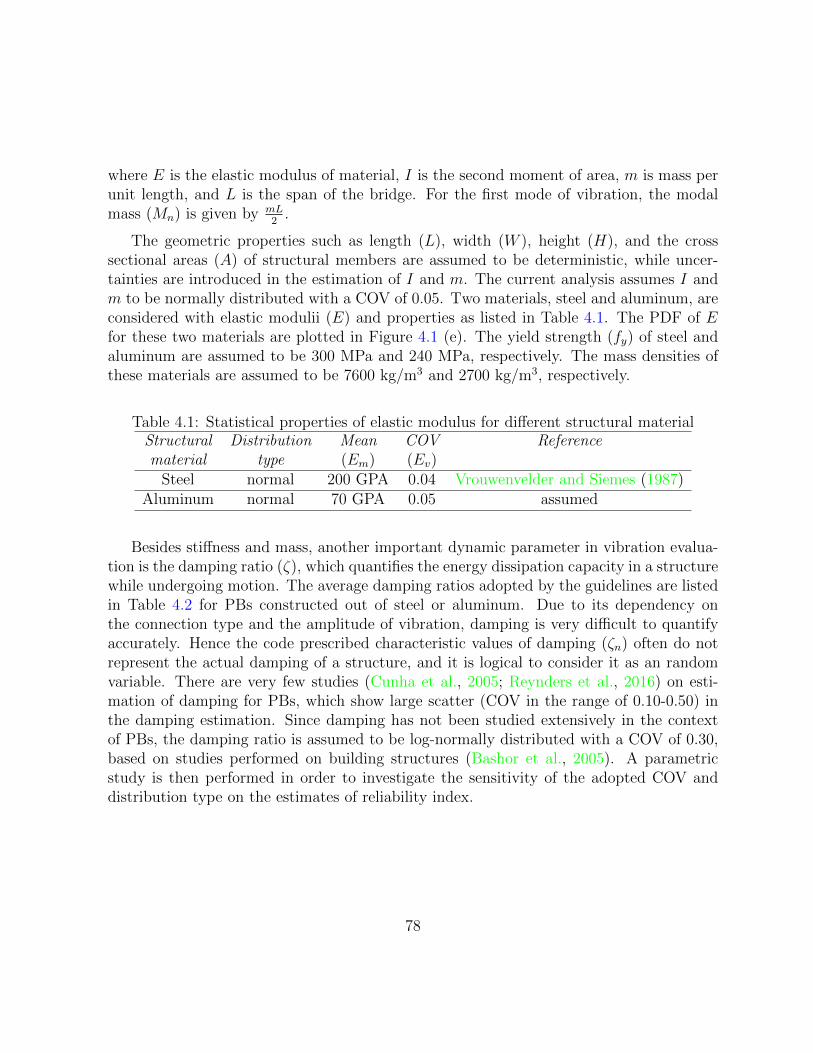
where E is the elastic modulus of material, I is the second moment of area, m is mass perunit length, and L is the span of the bridge. For the first mode of vibration, the modalmass (Mn) is given by mL

2.

The geometric properties such as length (L), width (W ), height (H), and the crosssectional areas (A) of structural members are assumed to be deterministic, while uncer-tainties are introduced in the estimation of I and m. The current analysis assumes I andm to be normally distributed with a COV of 0.05. Two materials, steel and aluminum, areconsidered with elastic modulii (E) and properties as listed in Table 4.1. The PDF of Efor these two materials are plotted in Figure 4.1 (e). The yield strength (fy) of steel andaluminum are assumed to be 300 MPa and 240 MPa, respectively. The mass densities ofthese materials are assumed to be 7600 kg/m3 and 2700 kg/m3, respectively.

Table 4.1: Statistical properties of elastic modulus for different structural materialStructural Distribution Mean COV Referencematerial type (Em) (Ev)

Steel normal 200 GPA 0.04 Vrouwenvelder and Siemes (1987)Aluminum normal 70 GPA 0.05 assumed

Besides stiffness and mass, another important dynamic parameter in vibration evalua-tion is the damping ratio (ζ), which quantifies the energy dissipation capacity in a structurewhile undergoing motion. The average damping ratios adopted by the guidelines are listedin Table 4.2 for PBs constructed out of steel or aluminum. Due to its dependency onthe connection type and the amplitude of vibration, damping is very difficult to quantifyaccurately. Hence the code prescribed characteristic values of damping (ζn) often do notrepresent the actual damping of a structure, and it is logical to consider it as an randomvariable. There are very few studies (Cunha et al., 2005; Reynders et al., 2016) on esti-mation of damping for PBs, which show large scatter (COV in the range of 0.10-0.50) inthe damping estimation. Since damping has not been studied extensively in the contextof PBs, the damping ratio is assumed to be log-normally distributed with a COV of 0.30,based on studies performed on building structures (Bashor et al., 2005). A parametricstudy is then performed in order to investigate the sensitivity of the adopted COV anddistribution type on the estimates of reliability index.

78

Table 4.2: Average damping ratios for steel/aluminumDesign Codes Damping (%)ISO 10137 0.5Eurocode 5 —British National Annex 0.5

SETRA 0.4

4.2 Range of design variables

4.2.1 Structural configurations

In order to quantify the level of reliability embodied in the existing guidelines, ranges ofdesign parameters in terms of structural configurations and traffic scenarios are consideredto reflect the design space of variables. For this purpose, the design configurations of PBsare established based on descriptions of the geometric properties of PBs around the world(Adeli, 2016). Four length to width ratio combinations are considered: L/W = [10, 15, 20,25], along with six widths: W = [1.0, 1.5, 2.0, 2.5, 3.0, and 4.0 m]. Two length to heightratios (L/H) are considered, depending on the length of the bridge. If L ≤ 20, L/H is(0.602L− 0.724) and (0.394L− 0.417). For 20 < L ≤ 40, L/H is 10 and 12. For L > 40,L/H is 12 and 18. The cross sectional areas (A) for the top and bottom chords are assumedto be the same, with 16 configurations ranging from 0.001 to 0.04 m2. The cross sectionalareas of the diagonals are assumed to be equal to that of the chords. Two configurationsfor deck thickness are assumed: 0.018 and 0.035 m. The second moments of area (In) inthe vertical and lateral directions are estimated as 4AH2

4and 2AW 2

4, respectively.

4.2.2 Design traffic

The design traffic corresponding to serviceability design is the normal traffic on a bridge,i.e., frequently occurring traffic scenarios such as daily commuters. Serviceability limitstate (SLS) design does not consider the extreme or rare design events, unlike ULS design.As discussed in Section 2.2, most of the guidelines except Eurocde 5 account for normaltraffic sizes, which vary based on the routes and usage of the PBs. In general, the normaltraffic size may range from sparse (around 0.2 P/m2) to very dense or heavy traffic (around1.0 P/m2) depending on the usage and route. The probable traffic levels to be consideredfor designing different PB classes by the guidelines have already been reviewed in Section2.2, which are summarized again here in Table 4.3. ISO 10137 does not provide any specific

79

design traffic size but points to the situations to be considered for the design. Eurocode5 suggests a 0.6 P/m2 density or 13 distinct pedestrians in a group. The British NationalAnnex and SETRA specify four traffic classes depending on usage, ranging from seldomused (negligible crowd density) to frequently used (heavy traffic).

Table 4.3: Traffic classes in various guidelinesCodes Traffic classISO 10137Case I (8 to 15 P) average pedestrian flowCase II (>15 P) streams of pedestriansCase II occasional festive or choreographic eventsEurocode 5 13 (group) or 0.6 P/m2 (crowd)British NationalAnnex to Eurocode 1Class A (2 P or 0 P/m2): rural locations seldom usedClass B (4 P or 0.4 P/m2): suburban location with occasional

variations in pedestrian loading intensityClass C (8 P or 0.8 P/m2): urban routes subject to significant

variation in daily usageClass D (16 P or 1.5 P/m2): primary access to major public assembly

SETRA (2006)Class I (1.0 P/m2): urban PB subjected to very heavy traffic frequentlyClass II (0.8 P/m2): urban PB with occasionally loaded throughout

bearing areaClass III (0.5 P/m2): PB for standard use, that will never be loaded

throughout its bearing areaClass IV: seldomly used PB (no dynamic assessment)

Besides frequently occurring traffic, a PB can be subjected to rare or in-frequent traffic.This may occur once in the lifetime of the bridge, e.g., during inauguration, sometimeswith densities around 1.5 P/m2 (Very heavy traffic), or periodically due to re-occurringevents. Even though rare traffic is typically not considered in SLS design, it can stillresult in significant economic losses (e.g., the LMB incident in 2001). On the other hand,designing solely based on such rare events may not be economical. To overcome suchissues, comfort classes or limiting accelerations (aln) based on the expected occurrence ofthe design traffic have been proposed (Heinemeyer et al., 2009). The choice of comfort classis flexible and depends on the owner. However, this idea has not yet been adopted by most

80

standards. ISO 10137 and Eurocode 5 use a single limiting acceleration (aln), while theBritish National Annex proposes aln based on site usage, route redundancy and the heightof structure, which implicitly takes care of the traffic size based on PB class. SETRAadopts four different comfort classes (Table 2.4), but does not consider traffic dependentcomfort criteria. In the current study, the mean comfort classes for pedestrians, aln = 1.0m/s2 (vertical) and aln = 0.3 m/s2 (lateral) in Table 2.4, are assumed for the reliabilityanalysis based on SETRA.

As reported in Table 4.3, there is a large variation in the traffic classes based on theusage recommended by various standards. The British National Annex and SETRA pro-vide four PB classes. However, the specified design densities corresponding to these classesare not consistent and furthermore, these standards neglect design densities less than 0.4P/m2 (British National Annex) and 0.5 P/m2 (SETRA). The current study adopts SETRAcrowd densities of 0.5-1.0 P/m2. Additionally, a new class corresponding to 0.2 P/m2 isintroduced in the current study. All of the structures are designed for the specified designdensity corresponding to the class and the reliability results in each class are generatedincluding results for other crowd densities expected during the lifetime of the structure,such as rare events with a density of 1.5 P/m2. The calculation of reliability indices andcorresponding results are presented and discussed in the following sections.

Table 4.4: PB classes and corresponding traffic sizes for the reliability analysisPB class Traffic situations Crowd density (P/m2)Class I PB for seldom use 0.2Class II PB for standard use in suburban area 0.5Class III urban PBs with occasionally loaded 0.8

throughout the bearing areaClass IV urban PBs linking the major public assembly 1.0

4.3 Calculation of reliability index

Reliability analysis starts with formulating the limit state function encompassing the designrandom variable space. For the SLS design of PBs under excessive vibration throughEquation 3.6, the limit state function g(X) by the existing design guidelines can be writtenas:

g(X) = al −2SN(E, I,m, ζ)Gαm

πLmζ= 0 (4.3)

81

where, the multiplication factor (SN) (refer to Table 3.8) is a function of E, I, m, andζ for the British National Annex and SETRA. For Eurocode 5, it depends on E, I, andm, while for ISO 10137, it is a constant. X is the vector of random variables consisting of[al, G, αm, ζ, E, I, m] for all of the guidelines except ISO 10137, which only considers[al, G, αm, ζ, m]. The limit state function g(X) defines the boundary dividing the failureand safe domains, given by:

Πf = x|g(x) ≤ 0

Πs = x|g(x) > 0(4.4)

where Πf and Πs are, respectively, the failure and safe domains. The failure probability isevaluated using:

Pf = P [g(x) ≤ 0] =

∫Πf

fx(x)dx (4.5)

The failure probability is related to the reliability index (β) by the following expression(Cornell, 1969):

Pf = Φ(−β) (4.6)

A total of 1536 geometric configurations are analyzed and only those configurationspassing the ultimate limit state design check for bending, as well as the serviceabilitychecks, were retained for the ensuing reliability analysis. The steps of the analysis are asfollows:

1. Static design check: Given the material properties and section geometry, a quickcheck for the ultimate bending stress is performed to exclude any failing combinationsfrom the 1536 geometric configurations for each material. The bending stress iscalculated under the factored dead (self-weight) and pedestrian induced live load(CAN/CSA S6, 2011) and subsequently compared with the factored critical limitstress (0.9fy) for the material.

2. Serviceability design check: For those designs retained in Step 1, the fundamentalfrequency is estimated through Equation 4.2 and compared with the critical rangesin Table 2.3. Serviceability design checks (Equation 3.5) are performed for thosefalling within these critical limits under design loading conditions for the assumedPB classes. To better understand the level of economy reached, a design factor isdefined here as follows:

φs =al

2SNGnαmn

πLmnζn

≥ 1.0 (4.7)

82

For optimally designed structures through Equation 3.5, this factor should be close to1.0 and an increase in this factor means higher reliability. The current study focusesonly on the optimally designed configurations, hence φs is restricted between 1.0 to1.1 during the deterministic design check.

3. Reliability evaluation: The optimally designed configurations are retained for thereliability analysis. Three standard techniques are employed for the calculation of β:Monte Carlo simulation (MCS), the advanced first-order second-moment (AFOSM)and the second-order reliability method (SORM). The MCS calculation is consideredas the benchmark and the indices obtained using the more computationally efficientAFOSM and SORM are compared with the results obtained using MCS.

The reliability index (β) calculated using AFOSM is also known as the modified Ha-sofer and Lind reliability index (Hasofer and Lind, 1974; Rackwitz and Flessler, 1978). Adetailed review of the steps to estimate β using this method are well documented in texts,e.g., in Nowak and Collins (2012). At its core, this method involves converting all non-normal distributions of random variables to equivalent normal distributions through theRackwitz-Fiessler procedure (Rackwitz and Flessler, 1978), followed by a transformationof the random variables to the standard normal space using:

zi =xi − µxiσxi

(4.8)

where the search for the most probable point or the design point is performed (z∗i ). Inthis equation, xi is the random variable with mean and standard deviation as µxi and σxi .β is estimated through iterative procedure, which requires solving the following (2n + 1)simultaneous equations with (2n+1) unknowns, β, α1, α2, ...., αn, z

∗1 , z∗2 , ...., z

∗n:

αi =− ∂g∂zi|z∗i√∑n

i=1( ∂g∂zi|z∗i )2

(4.9)

z∗i = βαi (4.10)

g(X) = 0 (4.11)

with, i = 1, 2, ...., n. The derivatives of the limit function with respect to each basic variablein the reduced space are evaluated at the design points (z∗i ) to estimate the sensitivity coef-ficients (αi), which represents the weightage of each random variable in the limit function.

83

The current study follows the matrix procedure presented in Nowak and Collins (2012) toestimate β.

AFOSM is generally acknowledged to be the simplest reliability analysis method, how-ever it approximates the curvature of the nonlinear limit state function by using onlya first-order approximation at the minimum distance point. Hence the accuracy of thismethod depends on the degree of nonlinearity of the limit state in the vicinity of theminimum distance point. Through including the second-order terms, SORM improvesthe reliability calculations compared to AFOSM. In the current study, the closed-formsolution for estimating the second order reliability index using the theory of asymptoticapproximations is adopted (Breitung, 1984), which is given by:

βSORM = −Φ−1[Φ(−βAFOSM)n−1∏i=1

(1 + βAFOSMKi)−1/2] (4.12)

where, Ki denotes the principal curvatures of the the limit state function at the minimumdistance point and is estimated as the eigen values of matrix A, whose elements aij aredefined by:

aij =(RDRt)ij|G|

, where, i, j = 1, 2, ..n− 1 (4.13)

Here, D is the n× n second-derivative matrix of the limit state function estimated in thestandard normal space evaluated at design points, R is the rotation matrix, and |G| isthe length of the gradient vector (first order differentiation of the limit state function withrespect to the random variables) in the standard normal space.

Both AFOSM and SORM require that the limit function in Equation 4.3 to be smoothand differentiable admitting up to and including second order derivatives. The factorskvert, khor, k(fv) and ψ (ψv or ψl) in Figures 2.9, 2.10 and 2.11 are not smooth functionswith respect to the structural frequency, fn, which is again a function of E, I, and m(Equation 4.2). This issue is addressed by performing the reliability analysis region-wise,on the frequency scale. First, the appropriate resonant harmonic is selected for evaluationbased on the mean frequency of the structure and the appropriate mean values of αm areselected. k(fv) in Figure 2.10(a) is smooth and continuous function of structural frequencywithin the frequency ranges corresponding to a particular harmonic (e.g., fn ≤ 2.8 for first

84

harmonic) and can be approximated using smooth polynomials as follows:

k(fv) =

−0.07128f 7n + 0.6776f 6

n − 2.202f 5n + 2.464f 4

n

+0.4139f 3n − 1.779f 2

n + 0.8538fn − 0.1049 if fn ≤ 2.8

−0.03033f 5n + 0.6949f 4

n − 6.116f 3n + 25.7f 2

n

−51.31fn + 39.67 if 2.8 < fn ≤ 5.6

0.05376f 3n − 1.128f 2

n + 7.48fn − 14.95 if fn > 5.6

(4.14)

kvert, khor, and ψ are not smooth for the entire range of frequencies corresponding toa particular harmonic. Rather, they are piece-wise linear functions for different rangeswithin a particular harmonic region. For example, ψv in Figure 2.11 (a) is not smooth andcontinuous in the range 1.0 ≤ fn ≤ 2.6 of first harmonic, but piece-wise linear function of fnin the ranges 1.0 ≤ fn ≤ 1.7, 1.7 ≤ fn ≤ 21 and 2.1 ≤ fn ≤ 2.6. Hence, reliability analysisis conducted within the linear zones corresponding to these variables. Furthermore, thesefactors approach zero, e.g., ψv in Figure 2.11 (a) at 1.0, 2.6, or 5.0 Hz. In order to avoidnumerical issues resulting from the regions close to zero, their values are assumed to bevery small instead of exactly zero.

Unlike other guidelines, SETRA estimates the response of a PB with and withoutthe added mass of pedestrians. Hence two values of responses (aN in equation (3.4))are calculated using this guideline and the maximum of the two responses is used forserviceability design check. Similarly, the reliability index β is also estimated with andwithout considering the added mass of pedestrians, β1 and β2 respectively and the minimumof these two β values is retained for analysis, i.e.,

β = min(β1, β2) (4.15)

4.4 Reliability analysis

4.4.1 Reliability-based design criteria

In reliability-based design, codes and standards are generally evaluated based on two cri-teria: sufficiency and uniformity over the range of designs covered by the respective codesand standards. The sufficiency criterion requires designing to an acceptable level of safety,usually represented by the target reliability index, βt, while the uniformity criterion ensuresuniform reliability of βt across all the designed applications. The issue of determining targetSLS reliability levels for PBs has not been studied in the literature. Generally applicable

85

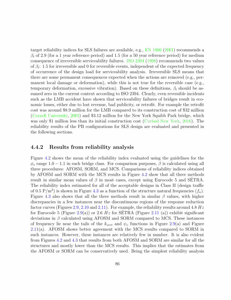
target reliability indices for SLS failures are available, e.g., EN 1990 (2001) recommends aβt of 2.9 (for a 1 year reference period) and 1.5 (for a 50 year reference period) for mediumconsequence of irreversible serviceability failures. ISO 2394 (1998) recommends two valuesof βt: 1.5 for irreversible and 0 for reversible events, independent of the expected frequencyof occurrence of the design load for serviceability analysis. Irreversible SLS means thatthere are some permanent consequences expected when the actions are removed (e.g., per-manent local damage or deformation), while this is not true for the reversible case (e.g.,temporary deformation, excessive vibration). Based on these definitions, βt should be as-sumed zero in the current context according to ISO 2394. Clearly, even reversible incidentssuch as the LMB accident have shown that serviceability failures of bridges result in eco-nomic losses, either due to lost revenue, bad publicity, or retrofit. For example the retrofitcost was around $8.9 million for the LMB compared to its construction cost of $32 million(Cornell University, 2005) and $3.12 million for the New York Squibb Park bridge, whichwas only $1 million less than its initial construction cost (Curbed New York, 2016). Thereliability results of the PB configurations for SLS design are evaluated and presented inthe following sections.

4.4.2 Results from reliability analysis

Figure 4.2 shows the mean of the reliability index evaluated using the guidelines for theφs range 1.0− 1.1 in each bridge class. For comparison purposes, β is calculated using allthree procedures: AFOSM, SORM, and MCS. Comparisons of reliability indices obtainedby AFOSM and SORM with the MCS results in Figure 4.2 show that all three methodsresult in similar mean values of β in most cases, except using Eurocode 5 and SETRA.The reliability index estimated for all of the acceptable designs in Class II (design trafficof 0.5 P/m2) is shown in Figure 4.3 as a function of the structure natural frequencies (fn).Figure 4.3 also shows that all the three methods result in similar β values, with higherdiscrepancies in a few instances near the discontinuous regions of the response reductionfactor curves (Figures 2.9, 2.10 and 2.11). For example, the reliability results around 4.8 Hzfor Eurocode 5 (Figure 2.9(a)) or 2.6 Hz for SETRA (Figure 2.11 (a)) exhibit significantdeviations in β calculated using AFOSM and SORM compared to MCS. These instancesof frequency lie near the tails of the kvert and ψv functions in Figure 2.9(a) and Figure2.11(a). AFOSM shows better agreement with the MCS results compared to SORM insuch instances. However, these instances are relatively few in number. It is also evidentfrom Figures 4.2 and 4.3 that results from both AFOSM and SORM are similar for all thestructures and mostly lower than the MCS results. This implies that the estimates fromthe AFOSM or SORM can be conservatively used. Being the simplest reliability analysis

86

method and computationally efficient, β results obtained using AFOSM are only reportedfor further analysis.

I II III IV-0.8

-0.6

-0.4

-0.2

β

ISO 10137

I II III IV-0.8

-0.6

-0.4

-0.2

Eurocode 5

I II III IVFootbridge classes

-0.8

-0.6

-0.4

-0.2

β

British National Annex (group)


-0.8

-0.6

-0.4

-0.2

British National Annex (crowd)


-0.8

-0.6

-0.4

-0.2

β

SÉTRA

AFOSM

SORM

MCS

(a) (b)

(e)

(d)(c)

Figure 4.2: Mean of reliability indices estimated for all the designs satisfying ψs = 1.0−1.1,using three reliability methods for different classes: (a) ISO 10137, (b) Eurocode 5, (c)British National Annex (group), (d) British National Annex (crowd), and (e) SETRA

Figure 4.3 also shows that the frequency range and the number of configurations satis-fying the SLS design are different amongst the guidelines. This is due to inconsistencies inthe design criteria as discussed in the previous sections and hence the designs satisfying theSLS design check according to these standards. For instance, both Eurocode and SETRAconsider 5 Hz as the upper bound of the critical frequency range (for only the first twoharmonics of resonance), while ISO 10137 and British National Annex have upper boundsof 12 Hz (first five harmonics) and 8 Hz (first three harmonics), respectively. Hence, sig-

87

nificantly more configurations are available for ISO 10137 and the British National Annexcompared to others. Furthermore, being conservative compared to SETRA, fewer config-urations are available for Eurocode 5 (Figures 4.3 (b) and (e)), although they have similarcritical frequency ranges. Similarly, ISO 10137 has fewer configurations compared to theBritish National Annex (Figures 4.3 (a), (c) and (d)). The results in Figure 4.4 for Class IVwith higher design traffic density (1.0 P/m2) underscore the same aforementioned issues.

2 4 6 8 10 12-0.8

-0.6

-0.4

-0.2

β

ISO 10137

1 2 3 4 5

-0.5

0Eurocode 5

2 4 6 8Structural frequency (Hz)

-0.8

-0.6

-0.4

-0.2

β



-0.8

-0.6

-0.4

-0.2


1 2 3 4 5Structural frequency (Hz)

-0.8

-0.6

-0.4

-0.2

β

SÉTRA

AFOSM

SORM

MCS

(e)

(c) (d)

(a) (b)

Figure 4.3: Reliability index as a function of structural frequency for Class II bridges undera design traffic of 0.5 P/m2: (a) ISO 10137, (b) Eurocode 5, (c) British National Annex(group), (d) British National Annex (crowd), and (e) SETRA.

88

2 4 6 8 10 12-1

-0.5

0β

ISO 10137

1 2 3 4 5-1

-0.5

0Eurocode 5


-1

-0.5

0

β



-1

-0.5

0British National Annex (crowd)


-1

-0.5

0

β

SÉTRA

AFOSMSORMMCS

(e)

(c) (d)

(b)(a)

Figure 4.4: Reliability index as a function of structural frequency for Class IV bridgesunder a design traffic of 1.0 P/m2: (a) ISO 10137, (b) Eurocode 5, (c) British NationalAnnex (group), (d) British National Annex (crowd), and (e) SETRA.

Uniformity criteria

The uniformity criteria are evaluated across all the bridge classes as well as across allthe design applications corresponding to each bridge class. The maximum and minimumreliability index (βmax and βmin) of all the designed applications corresponding to eachPB class is shown in Figure 4.5. The results show that the reliability levels embodied invarious guidelines are not uniform over the PB classes, except for the British NationalAnnex (group), which results in fairly uniform reliability across the four classes. Thisnon-uniformity in the reliability levels can be explained through Figures 4.3 and 4.4. Theprimary reason is the different structural configurations passing the optimality condition

89

for different classes. For example, in SETRA, the design traffic proportionally increaseswith the class, and hence configurations with small values of ψv (tails of the curve inFigure 2.11(a)) satisfy the serviceability design checks as shown in Figures 4.3 (e) and 4.4(e). Aside from the different PB configurations (i.e., span, width, height, mass, etc.), thedifferent numbers of PB configurations passing the deterministic serviceability design is alsoone of the reasons for the non-uniform reliability levels across the different PB classes. Forexample, PB Class II has 26 configurations (Figure 4.3 (e)) available for reliability analysis,while Class IV has 3 (Figure 4.4 (e)) in the case of SETRA. In order to assess the uniformityin the β values over all of the PB configurations for a specific class, βrange = βmax − βmincan be estimated as reported in Table 4.5. It is observed from this table and Figure 4.5that β has a significant spread across different PB configurations for some PB classes suchas Class I (SETRA) or Class II (Eurocode 5). However, βrange is very small for ISO 10137,specifically for PB Class IV, which is due to the relatively fewer configurations that areavailable for analysis (Figure 4.4(a)).

Table 4.5: Ranges of reliability index (βrange = βmax − βmin) for different PB classesCodes Class I Class II Class III Class IVISO 10137 0.273 0.130 0.118 0.065Eurocode 5 0.158 0.362 0.197 0.393British National Annex (group) 0.329 0.319 0.330 0.326British National Annex (crowd) 0.368 0.391 0.380 0.178

SETRA 0.519 0.294 0.294 0.046

Sufficiency criteria

In order to examine the sufficiency achieved across PB classes, the minimum reliabilityindex, βmin in Figure 4.5 is compared with the target reliability (βt = 0). This comparisonshows that all the designs for a specified density do not satisfy the sufficiency criteria,i.e., βmin < βt with βmin in the range of −0.5 to −0.8 across the standards. However,the deviation from the target value is low. The sufficiency criteria is also investigated forother traffic situations expected during its lifetime, including rare events associated witha density of 1.5 P/m2. The minimum reliability index (βmin) obtained using the designedconfigurations for various classes are shown in Figure 4.6. The results show that all of thePB classes produce lower reliability levels when higher traffic densities occur, which is to beexpected. Amongst all of the standards, the British National Annex (crowd) and SETRAresult in the lowest reliability index, between -3.5 to -4.75 (close to a probability of failure,

90

Pf = 1) under rare events (1.5 P/m2) for Class I. In the case of SETRA, Classes II andIII results in βmin = −4.75 as well. In general, Classes I and III are shown to performpoorly for all the guidelines under such unexpected events. Hence, designs belonging tothese classes (I to III) are deemed insufficient. For Class IV, (with a design traffic of 1.0P/m2) most of the designs result in β close to -1.0 under rare events (corresponding to 1.5P/m2).

I II III IV-0.8

-0.6

-0.4

-0.2

β

ISO 10137

I II III IV-0.8

-0.6

-0.4

-0.2

Eurocode 5


-0.8

-0.6

-0.4

-0.2

β



-0.8

-0.6

-0.4

-0.2



-0.8

-0.6

-0.4

-0.2

β

SÉTRA

βmax

βmin

(b)

(d)(c)

(e)

(a)

Figure 4.5: Maximum and minimum reliability levels for designs satisfying ψs = 1.0− 1.1for different classes: (a) ISO 10137, (b) Eurocode 5, (c) British National Annex (group),(d) British National Annex (crowd), and (e) SETRA

91

0.5 1 1.5

-4-2024

β

ISO 10137

0.5 1 1.5

-4

-2

0

2

4Eurocode 5

0.5 1 1.5Crowd density (P/m2)

-4

-2

0

2

4

β

British National Annex (Group)


-4

-2

0

2

4British National Annex (Crowd)


-4

-2

0

2

4

β

SÉTRA

Class IClass IIClass IIIClass IV

(a) (b)

(c) (d)

(e)

Figure 4.6: Minimum reliability levels (βmin calculated for the PBs (φs = 1.0− 1.1) underdifferent design cases: (a) ISO 10137, (b) Eurocode 5, (c) British National Annex (group),(d) British National Annex (crowd), and (e) SETRA (red markers correspond to the designtraffic of the particular PB class)

Comparison of reliability results by the guidelines

The reliability indices obtained using all of the standards are summarized in Table 4.6.This Table shows the minimum and maximum values for the reliability index obtainedfor all the optimally designed (φs = 1.0− 1.1) configurations for different classes under allpossible traffic situations in their design life as well as the reliability levels achieved by thesePBs under design traffic conditions (in parenthesis). Clearly, such bounds are a subset thatonly encompasses the PB configurations considered in the current study. However, it isbelieved that these configurations cover a broad range of design applications in terms of

92

PB class and structural frequency. In comparing the ranges i.e., βmax and βmin underall possible traffic scenarios in Table 4.6, the various code provisions show disagreementin the β ranges for all classes. Among all of the guidelines, SETRA results in the mostunconservative estimates for βmin, with βmin as low as -4.75 for Class I to Class III PBs,which implies a probability of failure of approximately 1.0. While the design traffic forthese classes is 0.2 to 0.8 P/m2, the βmin corresponds to 1.5 P/m2 (rare traffic). However,SETRA has a different functional form for the equivalent number of pedestrians neq underdesign and rare traffic. For the design traffic case, neq is 10.8

√ζnN . It is 1.85

√N for rare

traffic. This results in very low β estimates compared to other guidelines, which have auniform functional form for all traffic densities for design or rare events.

Table 4.6: Summary of reliability results for different PB classes

CodesClass I Class II Class III Class IV

βmax βmin βmax βmin βmax βmin βmax βminISO 10137 -0.33 -2.88 0.48 -1.26 0.91 -0.96 1.37 -0.98

(-0.33) (-0.61) (-0.34) (-0.47) (-0.36) (-0.47) (-0.45) (-0.51)Eurocode 5 -0.31 -2.24 1.26 -1.75 1.92 -1.20 2.66 -1.07

(-0.31) (-0.47) (-0.06) (-0.42) (-0.18) (-0.38) (-0.07) (-0.47)British National -0.27 -2.89 0.47 -2.01 0.95 -1.42 1.19 -1.12Annex (group) (-0.33) (-0.66) (-0.33) (-0.64) (-0.32) (-0.65) (-0.32) (-0.65)British National -0.36 -3.42 0.85 -2.23 1.45 -1.56 1.70 -1.02Annex (crowd) (-0.36) (-0.72) (-0.32) (-0.71) (-0.32) (-0.70) (-0.31) (-0.49)

SETRA -0.22 -4.75 5.17 -4.75 2.06 -4.75 3.21 -0.62(-0.22) (-0.74) (-0.30) (-0.59) (-0.27) (-0.57) (-0.31) (-0.35)

Note: Numbers in parenthesis are the minimum and maximum values of reliabilityindices, estimated for the PB classes under the specified design traffic

Under design traffic (values in parenthesis in Table 4.6), ISO 10137 and Eurocode 5 showsignificant agreement in terms of βmin. This is likely due to the fact that the multiplicationfactors for both the codes are independent of ζ. Similarly, the SETRA estimates for ClassesI to III are close to the British national Annex (crowd), which has a functional form of themultiplication factor similar to SETRA. In terms of βmax, Eurocode 5 results in the mostconservative estimates and shows significant disagreement with other guidelines for ClassesII to IV. This disagreement is largely due to inconsistencies in the design methodologiesand hence the designed configurations available for reliability assessment.

93

4.4.3 Parametric study

Individual contributions from various random variables on the overall reliability level willhelp decide the most sensitive variables for future code calibration efforts. Moreover,appropriate information about the uncertainty in the design parameters is needed for codecalibration. While uncertainty models for the pedestrian excitation parameters, G and αm,are established in the literature, those for the structural variables and pedestrian’s comfortlimit under pedestrian bridge vibration are not explored. For example, uncertainty modelsfor I and m are not available and hence assumed here. The uncertainty models for ζ and alare adopted from the literature on occupant’s comfort in high rise buildings developed inthe wind engineering literature. Hence, a parametric study should be performed in order toinvestigate the sensitivity of the reliability estimation to these adopted uncertainty models.

Sensitivity to limit acceleration

Due to inter- and intra-subject variabilities, the limit acceleration al is associated withsignificant randomness. For the current study, al is assumed to be log-normally distributedwith a COV of 0.20, based on the literature on occupant’s comfort under wind-inducedvibration of high-rise building (Bashor et al., 2005). The sensitivity with respect to al isinvestigated and the results are shown in Figures 4.7 and 4.8. As shown in Figure 4.7, anincrease in the COV of al decreases the reliability levels for all of the guidelines and thechange in β with respect to COV is significant. Comparing the estimates of β for differentdistribution types of al, such as normal, log-normal and extreme value distributions inFigure 4.8, the lowest mean β values result from the use of the extreme value distributionand the highest from a normal distribution. However, the sensitivity of β to the distributiontype of al is negligibly small. The difference in the estimates obtained using an extremevalue distribution versus those obtained using a log-normal distribution is in the range of6% to 7%. On the other hand, difference in the estimates between normal and log-normaldistributions are in the range of 8% to 9%. As β is not sensitive to the distribution typeof al, for simplicity, a normal distribution is assumed for future calibration.

Sensitivity to structural variables

E, I, m, and ζ are the basic design variables corresponding to structure in Equation 4.3.E, I, and m, which are related to the geometric and material properties of the structure,are associated with low COVs. For the reliability analysis in the current study, a value of0.05 is assumed for I and m, while the uncertainty model for E is chosen from literature

94

for steel and assumed for aluminum. The reliability results including uncertainties in theseparameters are compared with the ones where E, I, and m are assumed deterministic.Figure 4.9 shows the mean reliability levels estimated for all the classes of PB. It is seen thatin most of the cases, uncertainties in these variables do not affect the reliability estimationsignificantly, mainly due to very low COVs of these parameters. The reliability estimationis sensitive to the uncertainty in E in some instances for Eurocode 5 and SETRA. ForClass II in Figure 4.10, it is evident that the impact of these variables on the reliabilityestimates is negligible for ISO 10137, since the multiplication factor is independent of theseparameters and the limit state function depends only on m. In other cases, the contributionof these parameters depends on the region in the response reduction factor curve in Figures2.9 to 2.11. In the tail regions, the contribution of E is significant, but uncertainties in Eproduce higher estimates for β. Based on these results, it is concluded that E, I, and mcan conservatively be treated as deterministic parameters for code calibration purposes.

Unlike E, I, and m, there is significant scatter associated with ζ, as reported in theliterature (Bashor et al., 2005) for building. However, there is little information availablespecific to PBs (Cunha et al., 2005; Reynders et al., 2016). For the current study, ζis assumed to be log-normally distributed with a COV of 0.30, based on the buildingliterature (Bashor et al., 2005). A sensitivity study is conducted in Figures 4.11 and 4.12,in order to determine the impact of the COV and distribution types for ζ on the reliabilityestimates. Figure 4.11 shows the mean reliability index achieved by all of the designedconfigurations for a particular class for various assumed COVs of ζ. An increase in theCOV for ζ decreases the reliability level in all of the guidelines. However, the rate ofchange in the mean β values is not significant with an increase in the COV value. Themean β values for different distribution types such as normal, log-normal and Weibull arecompared in Figure 4.12, which shows that the log-normal distribution for ζ produces thelowest mean β values.

It is also investigated in Figure 4.13 whether assuming E, I, m and ζ as deterministicquantities has any significant effect on the reliability estimates. This will help in reducingthe number variables for future calibration process. It is observed that the uncertaintiesin these variables do not contribute significantly into the reliability estimates excepts ina few instances for Eurcode 5. Nevertheless, deterministic structural variables leads tolower reliability estimates and thus is assumed for the code calibration purposes. It shouldbe noted that the current study is limited to truss type PBs constructed from steel andaluminum (metals). The sensitivity study should be performed for other types of PBs witha wider range of material properties in order to choose the most sensitive random variablesfor code calibration.

95

0.05 0.1 0.15 0.2 0.25-1

-0.5

0

β

ISO 10137

0.05 0.1 0.15 0.2 0.25-1

-0.5

0Eurocode 5

0.05 0.1 0.15 0.2 0.25COV of a

l

-1

-0.5

0

β


0.05 0.1 0.15 0.2 0.25COV of a

l

-1

-0.5


0.05 0.1 0.15 0.2 0.25COV of a

l

-1

-0.5

0

β

SÉTRA


(c) (d)

(a) (b)

(e)

Figure 4.7: Variation of mean reliability index with coefficients of variation for al fordifferent PB classes: (a) ISO 10137, (b) Eurocode 5, (c) British National Annex (group),(d) British National Annex (crowd), and (e) SETRA

96

I II III IV-0.6

-0.4

-0.2

β

ISO 10137

I II III IV-0.6

-0.4

-0.2

Eurocode 5

I II III IVFootbridge class

-0.6

-0.4

-0.2

β



-0.6

-0.4

-0.2



-0.6

-0.4

-0.2

β

SÉTRA

NormalLog-normalExtreme value

(e)

(c) (d)

(b)(a)

Figure 4.8: Variation of mean reliability index with different distribution of ζ for differentPB classes: (a) ISO 10137, (b) Eurocode 5, (c) British National Annex (group), (d) BritishNational Annex (crowd), and (e) SETRA

97

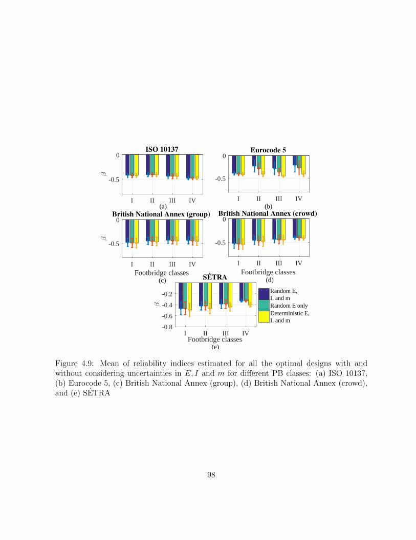
I II III IV

-0.5

0

β

ISO 10137

I II III IV

-0.5

0Eurocode 5


-0.5

0

β



-0.5



-0.8

-0.6

-0.4

-0.2

β

SÉTRA

Random E,I, and mRandom E onlyDeterministic E,I, and m

(a) (b)

(c) (d)

(e)

Figure 4.9: Mean of reliability indices estimated for all the optimal designs with andwithout considering uncertainties in E, I and m for different PB classes: (a) ISO 10137,(b) Eurocode 5, (c) British National Annex (group), (d) British National Annex (crowd),and (e) SETRA

98

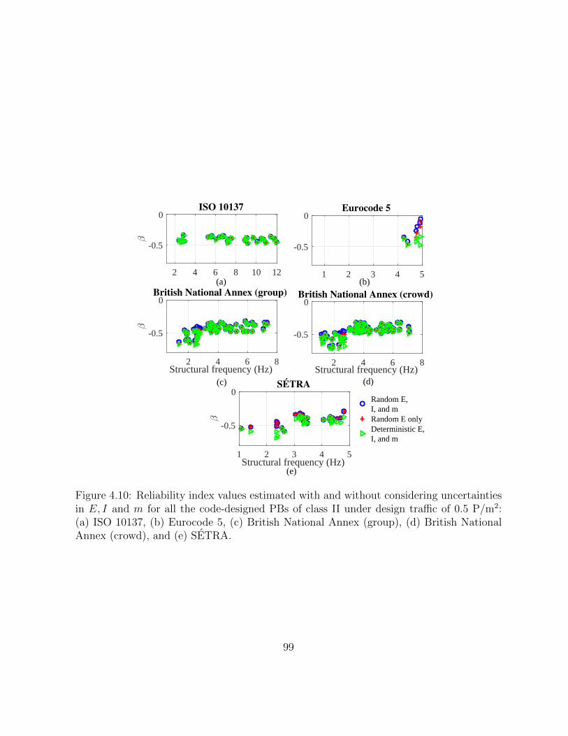
2 4 6 8 10 12

-0.5

0

β

ISO 10137

1 2 3 4 5

-0.5

0Eurocode 5


-0.5

0

β



-0.5



-0.5

0

β

SÉTRA

Random E,I, and mRandom E onlyDeterministic E,I, and m

(c) (d)

(e)

(a) (b)

Figure 4.10: Reliability index values estimated with and without considering uncertaintiesin E, I and m for all the code-designed PBs of class II under design traffic of 0.5 P/m2:(a) ISO 10137, (b) Eurocode 5, (c) British National Annex (group), (d) British NationalAnnex (crowd), and (e) SETRA.

99

0.05 0.1 0.15 0.2 0.25-0.6

-0.4

-0.2

β

ISO 10137

0.05 0.1 0.15 0.2 0.25-0.6

-0.4

-0.2

Eurocode 5

0.05 0.1 0.15 0.2 0.25COV of ζ

-0.6

-0.4

-0.2

β


0.05 0.1 0.15 0.2 0.25COV of ζ

-0.6

-0.4

-0.2


0.05 0.1 0.15 0.2 0.25COV of ζ

-0.6

-0.4

-0.2

β

SÉTRA


(e)

(a) (b)

(c) (d)

Figure 4.11: Variation of mean reliability index with coefficients of variation of ζ fordifferent PB classes: (a) ISO 10137, (b) Eurocode 5, (c) British National Annex (group),(d) British National Annex (crowd), and (e) SETRA

100

I II III IV-0.6

-0.4

-0.2

β

ISO 10137

I II III IV-0.6

-0.4

-0.2

Eurocode 5


-0.6

-0.4

-0.2

β



-0.6

-0.4

-0.2



-0.6

-0.4

-0.2

β

SÉTRA

Normal

Log-normal

Weibull

(d)

(e)

(c)

(b)(a)

Figure 4.12: Variation of mean reliability index with different distribution of ζ for differentPB classes: (a) ISO 10137, (b) Eurocode 5, (c) British National Annex (group), (d) BritishNational Annex (crowd), and (e) SETRA

101

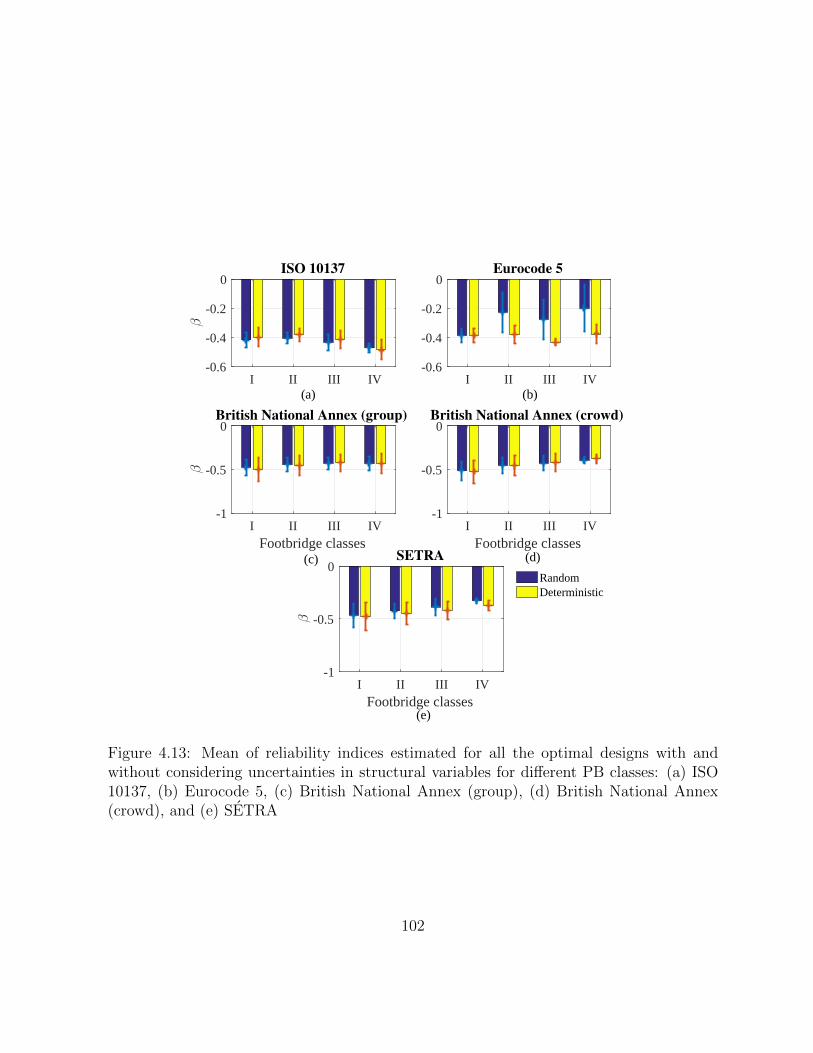
I II III IV-0.6

-0.4

-0.2

0

β

ISO 10137

I II III IV-0.6

-0.4

-0.2

0Eurocode 5


-1

-0.5

0

β



-1

-0.5



-1

-0.5

0

β

SETRA

RandomDeterministic

(a) (b)

(c) (d)

(e)

Figure 4.13: Mean of reliability indices estimated for all the optimal designs with andwithout considering uncertainties in structural variables for different PB classes: (a) ISO10137, (b) Eurocode 5, (c) British National Annex (group), (d) British National Annex(crowd), and (e) SETRA

102

4.4.4 Summary of key results from the reliability analysis

There are several broad observations resulting from the reliability-based evaluation of theguidelines presented in the previous sections. They are summarized as follows:

1. When a PB is designed for a particular crowd density, it does not satisfy the targetreliability index (βt) value of 0 under the design traffic. However, the deviation fromthe target value is low.

2. The PBs in Classes I to III fail to satisfy the minimum reliability requirement undervery heavy traffic during rare events such as inauguration, while past serviceabilityfailures have shown that such events have to be considered to avoid disproportionateeconomic losses and damaging negative public perception.

3. Due to inconsistencies in the design provisions, the guidelines result in significantdifferences in the reliability analysis.

4. A parametric study shows that the structural variables can be assumed deterministicfor conservative calibration process.

In the next chapter, these observations are addressed through a code calibration pro-cedure.

103

Chapter 5

Recommendations to improveexisting design provisions andreliability-based code calibration

Thus far, the focus has been on a comprehensive evaluation of the design provisions. Thischapter mainly deals with recommendations to improve design provisions so that theybetter align with experimental observations, both from a deterministic standpoint as wellas in a reliability-based framework. First, recommendations are proposed to improve theserviceability design outcomes by the guidelines and to reconcile the observed differencesamongst the guidelines and with the measurements. The serviceability outcomes afterincorporating the recommendations are then re-evaluated using the previous methodol-ogy. Finally, the existing as well as the recommended provisions are calibrated to achievesufficient reliability under all possible traffic conditions for different PB classes.

5.1 Recommendations for serviceability design

A general observation in Chapter 3 (Section 3.2.2) from the serviceability assessmentresults of the full-scale PBs under groups of pedestrians is that the vertical responses areconservative, while this is not the case for the lateral direction. Furthermore, significantinconsistencies are observed in the predictions by the guidelines. The main shortcomingsin the existing guidelines as observed in in Section 3.2.2 are summarized below:

• There is little guidance on correctly estimating walking speeds in crowd conditions.

104

The walking speed in a crowd depends on the traffic size. However, the guidelinesdo not consider traffic dependency, and hence of the structure with the relevantharmonics of walking frequency.

• The DLFs used are not uniform across the guidelines as shown in Table 3.9 eventhough the basic modelling approach and assumptions are largely aligned.

• They do not include a sufficient number of higher harmonics, although serviceabilityissues due to resonance with higher harmonics have been observed.

• The guidelines also adopt different multiplication factors, as described in Table 3.8,which lead to very different serviceability outcomes.

• Except for SETRA, the other guidelines do not consider the effect of added massfrom pedestrians in the response predictions.

5.1.1 Key design recommendations

An attempt is made in this section to address discrepancies summarized earlier throughincorporating the following key design recommendations within the basic design frameworkin Equation 3.5 adopted by the guidelines:

1. One of the shortcomings in all the guidelines is that they do not account for areduction of walking speed accompanying an increase in crowd density, which isimportant in order to choose the proper harmonic of walking frequency for resonanceas discussed in Section 3.2.2. In order to address this, the following relationshipbetween the crowd density (d), walking speed (v) and frequency, available in theliterature (Butz et al., 2008) can be incorporated:

v = 0.126d2 − 0.819d+ 1.779 (5.1)

fs = 0.7868v + 0.7886 (5.2)

Based on the expected walking frequency fs and the structural frequency (fn), theappropriate resonating harmonic (m) of walking frequency can be determined throughthe nearest integer of fn

fs. As the even harmonics contain relatively less energy in the

lateral direction, they are unlikely to create resonant conditions. Hence, the nearestodd harmonic can be considered in the lateral direction.

105

2. The DLFs (α′mn) by Brownjohn et al. (2004b) can be considered for response esti-mation in the vertical direction, because a number of higher harmonics have beenquantified in this work. The factors are 0.37fs− 0.42, 0.053, 0.042, 0.041, 0.027, and0.018 for the first six harmonics. The value for the seventh harmonic is currently notavailable and can be assumed to be 0.010. The recommended values for the first twoDLFs for the the lateral direction i.e. 0.05 and 0.01 can be regarded the same as theSETRA guideline. The DLFs for the next three higher harmonics are 0.023, 0.0043,and 0.011 as proposed by (Ricciardelli and Pizzimenti, 2007).

3. The multiplication factor SN proposed by the British National Annex in Table 3.8is recommended for the vertical direction, with a response reduction factor k(fv) =1.0. As the appropriate resonating harmonic is considered through traffic-dependentwalking speed, the response reduction factor k(fv), which takes care of the risk ofresonance, can be assumed as 1.0. Hence the recommended multiplication factor(S ′N) is

√(1 + γ(N − 1)) for concentrated load models under groups of pedestrians

and 1.8√

γNλ

for an uniformly distributed crowd model. The multiplication factor

proposed by SETRA (Table 3.8) with ψ = 1.0 i.e., neq or 10.8√

(ζnN) for d < 1.0

and 1.85√N for d ≥ 1.0, is recommended for the lateral direction. The pulsating

moving load model is recommended for transient loading (temporary, where groupscross the bridge together), while the uniformly distributed load model can be usedwhen the pedestrians are on the bridge long enough to create steady state conditions.

4. It is shown in Figures 3.16 and 3.17 for the SETRA guideline that the responsepredictions are sensitive to the added mass from pedestrians, specifically for densetraffic sizes. Hence, the effect of added mass from pedestrians on the response pre-dictions should be considered for other guidelines as well. It can be incorporatedas proposed by SETRA through estimating the modified structural frequency usingEquation 2.17.

These recommendations can be incorporated into the existing guidelines quite easily.For ISO 10137, the numerical coefficients in Table 2.5 can be calibrated with the newdynamic load factors α′mn and extended for higher harmonics in both the directions. The

factor C(N) in Equation 2.7 can be replaced withS′NN

. Similarly, simplified equations canbe derived for direct calculation of responses as proposed by Eurocode 5. Equations 2.9 and2.11 can be replaced with Pm

Mζfor the mth resonating harmonic. Pm is 200, 25, 20, 20, 15, 10,

and 5 respectively, for the first seven harmonics (m = 1 to 7) in the vertical direction, whileit is 20, 5, 10, 2, and 5 respectively, for the first five harmonics (m = 1 to 5) in the lateral

106

direction. The multiplication factors in Equations 2.8 (0.23kvertN) and 2.10 (0.18khorN)can be replaced by the recommended S ′N in the vertical and lateral directions. For BritishNational Annex, F0 and k(fv) in Equations 2.12 and 2.13 can be replaced with α′mnGn and1.0, respectively. In all of these guidelines, the response under the loaded structure shouldalso be estimated along with the unloaded case, and the higher of the two cases shouldbe used for design. In Equation 2.16 for SETRA, αmn, and ψneq should be replaced by,respectively, α′mn and S ′N for the first mode of vibration.

5.1.2 Effect of the recommended changes

To understand and quantify the effect of the proposed design recommendations on theexperimental results obtained from the two laboratory bridges studied in the current work,the proposed changes are incorporated into the basic design model in Equation 3.1. Firstthe response under a single pedestrian, as, is estimated using Equation 3.4. For the firstmode of vibration, the load Pi is given by 2α′mnGn

πfor both the moving concentrated and

the uniformly distributed load models. It should be noted however that Pi is α′mnGn

πfor

the second mode of vibration under uniformly distributed load, while it is the same forall the modes of vibration under concentrated moving load. Equation 3.1 is then appliedto estimate the response under crowd loading, with SN = S ′N . The higher of the tworesponses obtained from loaded (with added mass of pedestrians) and unloaded (withoutadded mass of pedestrians) structural conditions is considered for design.

The results of the recommended methodology are shown in Figures 5.1 (a) and (b)for both the 12.2 m and 22.9 m bridge specimens in the vertical direction. It is observedthat the modified results are significantly better than the responses originally predictedand shown in Figure 3.16. For the 12.2 m bridge specimen, the errors between measuredand predicted responses under all the traffic classes are bounded between 12% and 113%from their original values of 155% and 828% (ISO 10137). Similarly, for the 22.9 m bridgespecimen, these error bounds are 57% and 238% compared to their original values of −61%by the Eurocode 5 and 767% by the ISO 10137. Although the recommendations improvethe predictions of peak measurements, the trends are different between the experimentaland predicted responses as shown in Figures 5.1 (a) and (b). This is mainly due to thelevel of synchronization achieved during the tests, which is random, and depends on thecrowd size and human-structure interaction. However, this is deterministic and constantfor the simulated cases under all crowd sizes. The recommendations are proposed in thedeterministic framework similar to the existing guidelines. By taking the random natureof the level of synchronization into account, the predictions in trends observed during the

107

experiments can be vastly improved. However, this investigation is beyond the scope ofthe current thesis.

The lateral peak responses are shown in Figure 5.1 (c) and (d) for both the 12.2 m and22.9 m bridge specimens. As shown in Figure 3.17, the existing guidelines in general under-estimate the peak responses under medium to light traffic conditions. The recommendedresults in Figures 5.1 (c) and (d) are in better agreement with the measurements and yieldconservative estimates. In case of the 12.2 m bridge specimen, the errors in recommendedpredictions range from 164% to 270% while the existing guidelines have errors of −43%(Eurocode 5) to 41% (SETRA). Similarly, the errors for the 22.9 m bridge specimen rangefrom 18% to 71% while existing guidelines have errors ranging from −60% by the SETRAto 60% by the Eurocode 5.

It should be stressed that these recommendations are proposed to harmonize exist-ing design guidelines through DLFs and crowd multipliers in a relatively simple man-ner. However, they are drawn based on the experimental observations from only twoaluminum pedestrian bridges and hence there is significant scope to expand upon thisevidence through further testing on a broader variety of pedestrian bridges.

5.1.3 Reliability analysis after the proposed modifications

Along the same lines as described in the previous chapter (Section 4.2), reliability analysisis performed to investigate the effect of the proposed recommendations on the overallreliability of the PB configurations. For this purpose, a model error term (θen) is defined inEquation 5.3 to capture these proposed recommendations in the limit state design equation4.1:

θen =arecaN

(5.3)

where, arec is the response calculated through the procedure described in Section 5.1 andaN is the predicted response by the existing design provision before the recommendedchanges are incorporated. After introducing this model error term, the Equation 4.1 ismodified to:

aln ≥ θenSNGnαmnπMnζn

(5.4)

Subsequently, the modified SLS function can be wriiten as:

g′(X) = al − θe2SNGαmπLmζ

(5.5)

108

The characteristic value of θe (represented as θen in Equation 5.4) is estimated throughEquation 5.3 by estimating aN and arec. θe is assumed to be normally distributed witha mean equal to the predicted characteristic value from Equation 5.3 and COV of 0.10.This term could potentially be calibrated using experimental observations on various PBsin the future.

The reliability bounds (βmax and βmin ) are estimated for all the guidelines with theassumed uncertainties in the model error term (θe). Figure 5.2 shows these reliabilitybounds along with the bounds calculated using g(X) without θe in Equation 4.3. θe is seento have a significant impact on the reliability calculations using ISO 10137 and Eurocode5, which result in more conservative predictions compared to other guidelines as observedpreviously. The impact is less for the British National Annex, as the recommended pro-cedure already employs the same multiplication factor (SN) as the the British NationalAnnex in the vertical direction. These observations are also evident in Figure 5.3, whichshows β values for Class IV. The introduction of θe in the design equation results in alarger number of configurations passing the deterministic check for ISO 10137, Eurocode 5and SETRA, while the effect of θe on the design equation for the British National Annex isless. The sensitivity of the reliability results to the uncertainty in θe is also investigated inFigure 5.4. The reliability increases with an increase in the COV of θe. The assumption ofa deterministic θe results in the lowest estimates for reliability indices. Hence, to calibratethe guidelines with the modified design procedures, θe can be assumed deterministic.

5.2 Reliability-based calibration

A reliability-based evaluation of PBs showed that PBs designed for a particular crowddensity do not satisfy the target reliability level (βt) of 0 under design traffic conditions.However, the deviation from this target value is low. On the other hand, the evaluationresults also show that the PBs with lower design traffic (Class I to III) fail to satisfy theminimum reliability requirement under very dense traffic resulting from rare events suchas inauguration, etc. Past serviceability failure experiences have shown that such eventsmay have to be considered to avoid disproportionate economic loss and damaging negativepublic perception. This issue could be addressed by calibrating the design guidelines thatresult in an over-design for Class I to III bridges under design crowd densities, so that theyperform better during rare loading events.

It should be stressed that the reliability estimates in the previous chapter are basedon uniform comfort limits for pedestrians during both design and rare traffic conditions.As calibrating the PB classes to meet sufficiency during rare events could result in very

109

conservative designs, comfort limits based on the occurrence frequency of traffic are rec-ommended. This will ensure that economical designs can be achieved, while at the sametime resulting in acceptable performance during rare loading events. For this purpose,lower comfort limits as compared to the design case can be assigned for rare traffic density.As the reliability estimates are lower for bridge classes with lower design densities (Figure4.6), reliability required for calibrating the guidelines for sufficiency for the rare event willbe higher for such classes. Thus, the reliability required for calibration i.e., at the designlevel, will not be uniform across the PB classes. This can be resolved through calibratingthe design guidelines across all bridge classes with the same reliability as required for ClassI as this class results in the lowest reliability under the rare event or requires the largestreliability index for calibration as compared to other classes. However, this leads to anuneconomical design for classes with dense design densities such as III or IV, which can beimproved through establishing class-based design comfort limits.

To study this further, several cases are established in Table 5.1 based on different choicesof acceleration limits under both design and rare traffic events. A rare traffic density case of1.5 P/m2 (Heinemeyer et al., 2009) is adopted for analysis in addition to the design densitycorresponding to a bridge class (Table 4.4). In Table 5.1, D and R stands for design andrare events, respectively, where the reliability analysis is conducted during the respectiveevents. It should be noted that irrespective of the events D and R, the structures arefirst optimally designed for the design traffic density corresponding to a bridge class andthen the reliability analysis is performed for traffic density corresponding to the designor rare events. Two sets of cases are developed in Table 5.1: D1 to R15 and D2 to R25.In the first set, the structures are designed in accordance to the code prescribed limitacceleration values (aln) as in Table 2.4 for maximum comfort of pedestrians. The secondset is developed for uniform design performance across all PB classes, at the same timeproducing economic designs. In this case, mean comfort limits are desired for designingstructures corresponding to Class III and IV, while designs of Class I and II retain the codeprescribed limit accelerations similar to the first set. The mean comfort limit, aln = 1.0m/s2 by SETRA is chosen as the characteristic value for Class III and IV in the secondset. However, if this design limit (1.0 m/s2) for the second set is smaller than aln in Table2.4, aln in Table 2.4 are retained resulting in identical design limits for the first and secondsets.

For each set (i = 1, 2), 6 cases are developed, where only one is related to the designevent (Di), while the other 5 (Ri1 to Ri5) are for the rare event. The reliability analysis forcases Di and Ri1 are performed assuming the same comfort limits as adopted for design.Other 4 cases (Ri2 to Ri5) are developed based on different limit accelerations, rangingfrom 1.0 m/s2 to 2.5 m/s2, expected during the rare loading event. These acceleration

110

Table 5.1: Summary of cases based on comfort limits for pedestriansCases Acceleration limit (m/s2)Di Same as adopted in ith design caseRi1 Same as adopted in ith design caseRi2 Maximum of 1.0 m/s2 and the limit in ith design caseRi3 Maximum of 1.5 m/s2 and the limit in ith design caseRi4 Maximum of 2.0 m/s2 and the limit in ith design caseRi5 Maximum of 2.5 m/s2 and the limit in ith design case

*Di: reliability analysis for only design loading event**Rij: reliability analysis for both design and rare loading events

limits are taken from the mean or minimum comfort limits by SETRA. Moreover, if theseacceleration limits for the rare event are less than the one used for design i.e, the designlimit acceleration, this design limit for the rare traffic density is adopted for the calculationof reliability index.

As observed in Figures 4.3 and 4.4, very few configurations are available in certaininstances, for example, for Class IV. As the calibration process is being performed toachieve a higher reliability index, it is to be expected that very few configurations willsatisfy the calibrated design equation if the existing design space of configurations presentedin the previous chapter is retained. Hence, for the calibration process, the design spaceis extended (from Section 4.2) by incorporating 11 configurations for cross sectional arearanging from 0.05 m2 to 0.15 m2, 2 configurations of thickness (0.050 m and 0.075 m),1 configuration of width (5.0 m) and 1 length to width ratio (30). This results in anincrease in the total number of configurations from 1536 to 7560 for each material. Toexclude any failing combinations, the designs are checked for ultimate bending stress. Theretained configurations after the static check are employed for serviceability design andsubsequently the calibration process is carried out on the designs which pass this check.

5.2.1 Calibration process

Code calibration is a technique used to achieve a specified target reliability level (βt).Through such a calibration process, the variation in reliability indices across designs issignificantly minimized. The results form the parametric study in Section 4.4.3 suggeststhat uncertainties from the limit acceleration (al) and pedestrian load (G and αm) aresufficient for the calibration process. Hence, the modified SLS function for the design

111

guidelines can be written as:

g(X’) = al − θen2SN

πLmnζnGαm (5.6)

where, g(X’) represents the general limit state function for the design guidelines both with-out (existing) and with (improved) the model error term, θen. X’ is the vector consisting of3 random variables, [al, G, αm]. The calibration process will result in an estimate for thepartial factors corresponding to the random variables. These partial factors are nothingbut a scaling factor which allows the designer to convert the characteristic values of thebasic variables to the design value needed to achieve the target reliability. After calibra-tion, the design equation in 5.4 can be written in a load resistance factor design (LRFD)format (EN 1990, 2001):

γalaln ≥ θen2SN(γGGn)(γαmαmn)

πLmnζn(5.7)

where, γal , γG and γαm are the partial factors for the limit acceleration (al), pedestrian’sweight (G) and the dynamic load factor (αm). These factors together with the characteristicvalues of the design variables in Equation 5.7 will ensure an acceptable reliability index ofβt during design. The steps to estimate these factors for a given βt are discussed in thefollowing section.

Procedure to estimate the partial factors

The procedure to estimate partial factors, γal , γG and γαm , for a given βt, starts withformulating the limit state function and the design equation as in equations 5.6 and 5.7.The method allows at most two unknown mean values and the estimated factors becomeindependent of the mean values of those unknown variables. The current study assumesthat the mean of al is unknown so that the partial factors are independent of the meanlimit acceleration. The factors are estimated iteratively as follows (Nowak and Collins,2012):

1. Estimate the initial mean value of the unknown variable (al) from g(X’) = 0 (Equa-tion 5.6) at the mean values of other random variables.

2. Obtain the initial design point xi∗ assuming (n− 1) random variables where n is the

number of random variables and equals to 3 for the current analysis. Generally, themean values of the variables are a reasonable choice as the initial design point. Solvethe value of the remaining random variables from g(X’) = 0 (Equation 5.6). Thisensures that the design point is on the failure boundary.

112

3. For each design value corresponding to a non-normal distribution, determine theequivalent mean and standard deviation through the Rackwitz-Fiessler procedure(Rackwitz and Flessler, 1978).

4. Determine the partial derivative of the limit state function (g(X’)) with respect tothe reduced variables (zi) and estimate the sensitivity coefficients αi using Equation4.9.

5. Determine the new design point (zi∗) for the n−1 variables in the reduced coordinates

corresponding to a target reliability index βt using:

zi∗ = αiβt (5.8)

6. Covert the estimated design points in the previous step to the original coordinatesfor the n− 1 variables using:

xi∗ = µxi + zi

∗σxi (5.9)

7. Estimate the design value of the remaining random variable by using g(X’) = 0 atthe design point, where xi

∗ must be on the failure surface satisfying the limit statefunction g(X’∗) = 0.

8. Update the mean value of the unknown variable through using the following expres-sion:

µxi =xi∗

1 + αiβtVxi(5.10)

where Vxi is the COV of the unknown variable.

9. Repeat steps 3 to 8 until the sensitivity coefficients αi converges.

10. Estimate the partial factors for the random variable xi after achieving convergenceusing:

γxi =xi∗

xin(5.11)

where xin represents the characteristic value of the random variable.

113

Target reliability

As mentioned earlier code calibration in general, is performed to achieve an acceptablereliability level, known as target reliability, which is based on the consequence of failure,economic loss, etc. Along similar lines, the serviceability design provisions are calibratedhere to achieve acceptable performance not only at the design level, but also for rare loadingevents. For the purpose of calibration, which is conducted at the design level event, thetarget reliability should be known or established a priori. As a cost based analysis toestimate the target reliability (βt) is not performed here, an index βd known as the desiredreliability at the design event level is introduced. βd is estimated through iteration so thatthe mean reliability achieved by all the designs during the design as well as rare traffic ismore than 0, which is the proposed target reliability by ISO 2934 for sufficiency. Onceβd is estimated for each case in Table 5.1, then the corresponding partial factors can beassigned to Equation 5.7.

The overall implementation procedure is undertaken in two stages:

• Estimation of partial factors: The partial factors, γal , γG and γαm correspondingto Equation 5.7 are estimated for assumed βt levels ranging from 0.25 to 4.5 with anincrement of 0.25 though the steps discussed in the previous section.

• Estimation of desired reliability: The desired reliability (βd) is estimated itera-tively for each case in Table 5.1 as follows:

1. For an initial estimate of βd, a reliability analysis is first conducted for a trafficdensity corresponding to the case under consideration (Table 5.1) for Class I,designed according to Equation 5.4 for design density of 0.2 P/m2. The closestβt level (listed in the previous step) to the estimated reliability index is chosenas the desired reliability for the first iteration.

2. The structural configurations satisfying the static checks and the frequency lim-its are designed for Class I in accordance to the serviceability design equationin 5.7 with partial factors corresponding to the assumed βd from the previousstep, and those satisfying this equation are retained for reliability analysis.

3. Reliability analysis is performed on the limit state function in Equation 5.6following AFOSM method for all the optimally designed configurations. In caseof D1 or D2, the mean reliability index from all the designs is estimated onlyfor the design density (0.2 P/m2) and retained for the next step, epresented byβet. In the case of Ri1 to Ri1, both the design (0.2 P/m2) and rare (1.5 P/m2)

114

traffic densities are considered and two mean values of β corresponding to thedesign (βD) and rare (βR) traffic events are estimated. The minimum of thesereliability indices is retained for the next step as:

βet = min[βD, βR] (5.12)

4. If βet is less than 0, then steps 2 and 3 are repeated using βd as the next βt untilβet is greater than 0 and the corresponding βt is the desired reliability for theparticular case. On the other hand, if βet is greater than 0 at the first iteration,then steps 2 and 3 are repeated using βt from the previous step until βet is lessthan 0. Then, the final value of the desired reliability is βt + 0.25.

5. The partial factors corresponding to the estimated βd are the design partialfactors for the particular case in Table 5.1.

5.2.2 Results of calibration

Partial factors

The partial factors, γal , γG and γαm are first estimated for different target reliability indicesranging from 0.25 to 4.5 and reported in Table 5.2. It should be noted that while incrementsof βt are limited to 0.25, smaller increments can be employed using the same methodologyfor a more accurate estimation of the desired reliability.

Table 5.2 reports only one set of factors corresponding to a target reliability level asthe calibration process leads to identical factors for all the guidelines. Furthermore, thefactors are independent of the PB classes. It has been already discussed in the previouschapter that the main inconsistency amongst the guidelines lies in the multiplication factor,SN (Table 3.8) and limit acceleration, aln (Table 2.4), although they are based on thesame basic framework. However, the calibration process assumes SN as deterministic. Onthe other hand, as the procedure of calibration only requires known mean values from 2variables which are G and αm for the current analysis. Thus, despite different values of limitaccelerations employed by the guidelines, estimation of the partial factors are independentof the different values of limit acceleration. Furthermore, the distribution type and COVfor all the variables are identical in the guidelines. Due to these reasons, the factors acrossall the design provisions and all the PB classes are identical. Moreover, as the model errorterm is assumed deterministic, incorporation of this error term will not affect the partialfactors. It is also seen in Table 5.2 that the factors for the first harmonic is differentfrom the higher harmonics. This is due to the significantly higher COV (=0.40) for higher

115

Table 5.2: Partial factors corresponding to different target reliability index

βtm=1 m>1

γal γG γαm γal γG γαm

0.250 0.770 1.008 1.023 0.778 1.001 1.0810.500 0.742 1.031 1.044 0.758 1.018 1.1580.750 0.713 1.053 1.063 0.735 1.037 1.2291.000 0.683 1.075 1.082 0.711 1.056 1.2961.250 0.651 1.096 1.098 0.683 1.075 1.3581.500 0.617 1.116 1.113 0.654 1.094 1.4141.750 0.581 1.134 1.126 0.622 1.113 1.4662.000 0.544 1.150 1.138 0.588 1.131 1.5112.250 0.504 1.163 1.146 0.551 1.147 1.5502.500 0.463 1.173 1.153 0.511 1.161 1.5812.750 0.419 1.177 1.156 0.468 1.172 1.6043.000 0.373 1.177 1.156 0.422 1.177 1.6163.250 0.326 1.171 1.152 0.372 1.177 1.6163.500 0.277 1.159 1.143 0.319 1.170 1.6003.750 0.228 1.140 1.131 0.264 1.154 1.5664.000 0.179 1.116 1.113 0.206 1.130 1.5094.250 0.131 1.087 1.091 0.149 1.099 1.4274.500 0.085 1.055 1.065 0.094 1.062 1.317

harmonics of DLF values (m > 1) as compared to the first harmonic (COV=0.17). It shouldbe stressed that these factors will depend on the uncertainty models used for the randomvariables. Moreover, if the uncertainties from structural properties are incorporated, thefactors will not be consistent across the guidelines.

Desired reliability

After obtaining the partial factors with respect to a particular target reliability level inTable 5.2, βd is estimated through iteration for all the cases listed in Table 5.1. Figure5.5 shows βd estimated for cases D1 to R15, which are also reported in Table 5.3. As theestimation of βd is performed based on Class I of PBs and D2 to R25 are identical caseswith respect to D1 to R15 for this class of PBs, βd for cases D2 to R25 will remain the sameas those for D1 to R15. Hence, only the results corresponding to D1 to R15 are reportedhere.

116

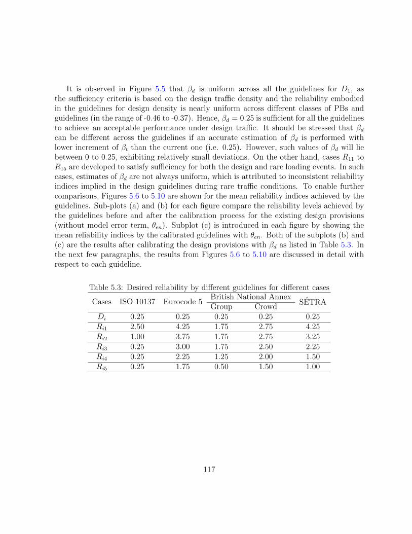
It is observed in Figure 5.5 that βd is uniform across all the guidelines for D1, asthe sufficiency criteria is based on the design traffic density and the reliability embodiedin the guidelines for design density is nearly uniform across different classes of PBs andguidelines (in the range of -0.46 to -0.37). Hence, βd = 0.25 is sufficient for all the guidelinesto achieve an acceptable performance under design traffic. It should be stressed that βdcan be different across the guidelines if an accurate estimation of βd is performed withlower increment of βt than the current one (i.e. 0.25). However, such values of βd will liebetween 0 to 0.25, exhibiting relatively small deviations. On the other hand, cases R11 toR15 are developed to satisfy sufficiency for both the design and rare loading events. In suchcases, estimates of βd are not always uniform, which is attributed to inconsistent reliabilityindices implied in the design guidelines during rare traffic conditions. To enable furthercomparisons, Figures 5.6 to 5.10 are shown for the mean reliability indices achieved by theguidelines. Sub-plots (a) and (b) for each figure compare the reliability levels achieved bythe guidelines before and after the calibration process for the existing design provisions(without model error term, θen). Subplot (c) is introduced in each figure by showing themean reliability indices by the calibrated guidelines with θen. Both of the subplots (b) and(c) are the results after calibrating the design provisions with βd as listed in Table 5.3. Inthe next few paragraphs, the results from Figures 5.6 to 5.10 are discussed in detail withrespect to each guideline.

Table 5.3: Desired reliability by different guidelines for different cases

Cases ISO 10137 Eurocode 5British National Annex

SETRAGroup Crowd

Di 0.25 0.25 0.25 0.25 0.25Ri1 2.50 4.25 1.75 2.75 4.25Ri2 1.00 3.75 1.75 2.75 3.25Ri3 0.25 3.00 1.75 2.50 2.25Ri4 0.25 2.25 1.25 2.00 1.50Ri5 0.25 1.75 0.50 1.50 1.00

117

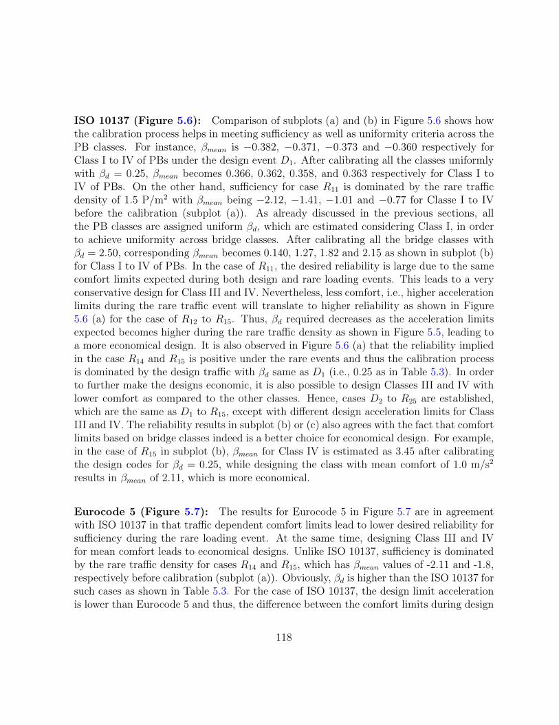
ISO 10137 (Figure 5.6): Comparison of subplots (a) and (b) in Figure 5.6 shows howthe calibration process helps in meeting sufficiency as well as uniformity criteria across thePB classes. For instance, βmean is −0.382, −0.371, −0.373 and −0.360 respectively forClass I to IV of PBs under the design event D1. After calibrating all the classes uniformlywith βd = 0.25, βmean becomes 0.366, 0.362, 0.358, and 0.363 respectively for Class I toIV of PBs. On the other hand, sufficiency for case R11 is dominated by the rare trafficdensity of 1.5 P/m2 with βmean being −2.12, −1.41, −1.01 and −0.77 for Classe I to IVbefore the calibration (subplot (a)). As already discussed in the previous sections, allthe PB classes are assigned uniform βd, which are estimated considering Class I, in orderto achieve uniformity across bridge classes. After calibrating all the bridge classes withβd = 2.50, corresponding βmean becomes 0.140, 1.27, 1.82 and 2.15 as shown in subplot (b)for Class I to IV of PBs. In the case of R11, the desired reliability is large due to the samecomfort limits expected during both design and rare loading events. This leads to a veryconservative design for Class III and IV. Nevertheless, less comfort, i.e., higher accelerationlimits during the rare traffic event will translate to higher reliability as shown in Figure5.6 (a) for the case of R12 to R15. Thus, βd required decreases as the acceleration limitsexpected becomes higher during the rare traffic density as shown in Figure 5.5, leading toa more economical design. It is also observed in Figure 5.6 (a) that the reliability impliedin the case R14 and R15 is positive under the rare events and thus the calibration processis dominated by the design traffic with βd same as D1 (i.e., 0.25 as in Table 5.3). In orderto further make the designs economic, it is also possible to design Classes III and IV withlower comfort as compared to the other classes. Hence, cases D2 to R25 are established,which are the same as D1 to R15, except with different design acceleration limits for ClassIII and IV. The reliability results in subplot (b) or (c) also agrees with the fact that comfortlimits based on bridge classes indeed is a better choice for economical design. For example,in the case of R15 in subplot (b), βmean for Class IV is estimated as 3.45 after calibratingthe design codes for βd = 0.25, while designing the class with mean comfort of 1.0 m/s2

results in βmean of 2.11, which is more economical.

Eurocode 5 (Figure 5.7): The results for Eurocode 5 in Figure 5.7 are in agreementwith ISO 10137 in that traffic dependent comfort limits lead to lower desired reliability forsufficiency during the rare loading event. At the same time, designing Class III and IVfor mean comfort leads to economical designs. Unlike ISO 10137, sufficiency is dominatedby the rare traffic density for cases R14 and R15, which has βmean values of -2.11 and -1.8,respectively before calibration (subplot (a)). Obviously, βd is higher than the ISO 10137 forsuch cases as shown in Table 5.3. For the case of ISO 10137, the design limit accelerationis lower than Eurocode 5 and thus, the difference between the comfort limits during design

118

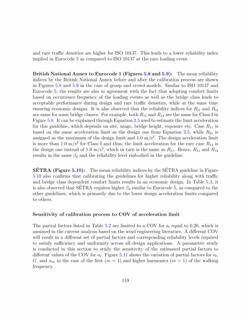
and rare traffic densities are higher for ISO 10137. This leads to a lower reliability indeximplied in Eurocode 5 as compared to ISO 10137 at the rare loading event.

British National Annex to Eurocode 1 (Figures 5.8 and 5.9): The mean reliabilityindices by the British National Annex before and after the calibration process are shownin Figures 5.8 and 5.9 in the case of group and crowd models. Similar to ISO 10137 andEurocode 5, the results are also in agreement with the fact that adopting comfort limitsbased on occurrence frequency of the loading events as well as the bridge class leads toacceptable performance during design and rare traffic densities, while at the same timeensuring economic designs. It is also observed that the reliability indices for Ri1 and Ri2

are same for some bridge classes. For example, both R11 and R12 are the same for Class I inFigure 5.8. It can be explained through Equation 2.5 used to estimate the limit accelerationfor this guideline, which depends on site, usage, bridge height, exposure etc. Case R11 isbased on the same acceleration limit as the design one from Equation 2.5, while R21 isassigned as the maximum of the design limit and 1.0 m/s2. The design acceleration limitis more than 1.0 m/s2 for Class I and thus, the limit acceleration for the rare case R12 isthe design one instead of 1.0 m/s2, which in turn is the same as R11. Hence, R11 and R12

results in the same βd and the reliability level embodied in the guideline.

SETRA (Figure 5.10): The mean reliability indices by the SETRA guideline in Figure5.10 also confirms that calibrating the guidelines for higher reliability along with trafficand bridge class dependent comfort limits results in an economic design. In Table 5.3, itis also observed that SETRA requires higher βd similar to Eurocode 5, as compared to theother guidelines, which is primarily due to the lower design acceleration limits comparedto others.

Sensitivity of calibration process to COV of acceleration limit

The partial factors listed in Table 5.2 are limited to a COV for al equal to 0.20, which isassumed in the current analysis based on the wind engineering literature. A different COVwill result in a different set of partial factors and corresponding reliability levels requiredto satisfy sufficiency and uniformity across all design applications. A parametric studyis conducted in this section to study the sensitivity of the estimated partial factors todifferent values of the COV for al. Figure 5.11 shows the variation of partial factors for al,G, and αm in the case of the first (m = 1) and higher harmonics (m > 1) of the walkingfrequency.

119

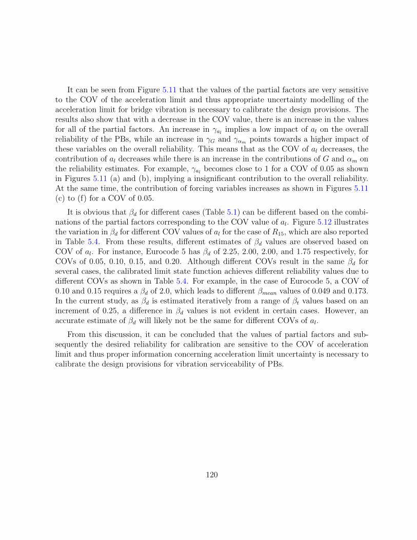
It can be seen from Figure 5.11 that the values of the partial factors are very sensitiveto the COV of the acceleration limit and thus appropriate uncertainty modelling of theacceleration limit for bridge vibration is necessary to calibrate the design provisions. Theresults also show that with a decrease in the COV value, there is an increase in the valuesfor all of the partial factors. An increase in γal implies a low impact of al on the overallreliability of the PBs, while an increase in γG and γαm points towards a higher impact ofthese variables on the overall reliability. This means that as the COV of al decreases, thecontribution of al decreases while there is an increase in the contributions of G and αm onthe reliability estimates. For example, γal becomes close to 1 for a COV of 0.05 as shownin Figures 5.11 (a) and (b), implying a insignificant contribution to the overall reliability.At the same time, the contribution of forcing variables increases as shown in Figures 5.11(c) to (f) for a COV of 0.05.

It is obvious that βd for different cases (Table 5.1) can be different based on the combi-nations of the partial factors corresponding to the COV value of al. Figure 5.12 illustratesthe variation in βd for different COV values of al for the case of R15, which are also reportedin Table 5.4. From these results, different estimates of βd values are observed based onCOV of al. For instance, Eurocode 5 has βd of 2.25, 2.00, 2.00, and 1.75 respectively, forCOVs of 0.05, 0.10, 0.15, and 0.20. Although different COVs result in the same βd forseveral cases, the calibrated limit state function achieves different reliability values due todifferent COVs as shown in Table 5.4. For example, in the case of Eurocode 5, a COV of0.10 and 0.15 requires a βd of 2.0, which leads to different βmean values of 0.049 and 0.173.In the current study, as βd is estimated iteratively from a range of βt values based on anincrement of 0.25, a difference in βd values is not evident in certain cases. However, anaccurate estimate of βd will likely not be the same for different COVs of al.

From this discussion, it can be concluded that the values of partial factors and sub-sequently the desired reliability for calibration are sensitive to the COV of accelerationlimit and thus proper information concerning acceleration limit uncertainty is necessary tocalibrate the design provisions for vibration serviceability of PBs.

120

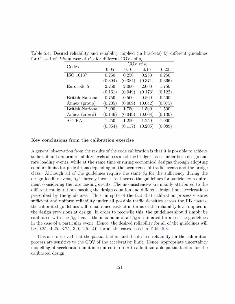
Table 5.4: Desired reliability and reliability implied (in brackets) by different guidelinesfor Class I of PBs in case of R15 for different COVs of al

CodesCOV of al

0.05 0.10 0.15 0.20ISO 10137 0.250 0.250 0.250 0.250

(0.394) (0.384) (0.371) (0.366)Eurocode 5 2.250 2.000 2.000 1.750

(0.161) (0.049) (0.173) (0.122)British National 0.750 0.500 0.500 0.500Annex (group) (0.205) (0.009) (0.042) (0.075)British National 2.000 1.750 1.500 1.500Annex (crowd) (0.146) (0.049) (0.008) (0.130)

SETRA 1.250 1.250 1.250 1.000(0.054) (0.117) (0.205) (0.089)

Key conclusions from the calibration exercise

A general observation from the results of the code calibration is that it is possible to achievesufficient and uniform reliability levels across all of the bridge classes under both design andrare loading events, while at the same time ensuring economical designs through adoptingcomfort limits for pedestrians depending on the occurrence of traffic events and the bridgeclass. Although all of the guidelines require the same βd for the sufficiency during thedesign loading event, βd is largely inconsistent across the guidelines for sufficiency require-ment considering the rare loading events. The inconsistencies are mainly attributed to thedifferent configurations passing the design equation and different design limit accelerationsprescribed by the guidelines. Thus, in spite of the fact that calibration process ensuressufficient and uniform reliability under all possible traffic densities across the PB classes,the calibrated guidelines will remain inconsistent in terms of the reliability level implied inthe design provisions at design. In order to reconcile this, the guidelines should simply becalibrated with the βd, that is the maximum of all βd’s estimated for all of the guidelinesin the case of a particular event. Hence, the desired reliability for all of the guidelines willbe [0.25, 4.25, 3.75, 3.0, 2.5, 2.0] for all the cases listed in Table 5.3.

It is also observed that the partial factors and the desired reliability for the calibrationprocess are sensitive to the COV of the acceleration limit. Hence, appropriate uncertaintymodelling of acceleration limit is required in order to adopt suitable partial factors for thecalibrated design.

121

0

1

2

3

Pea

k A

ccel

erat

ion

(m/s2 )

12.2 m

MeasurementRecommendedISO 10137Eurocode 5British NationalAnnexSÉTRA (Limit I)SÉTRA (Limit II)SÉTRA (Limit III)

0

1

2

3

4

522.9 m

0

1

2

3

Pea

k ac

cele

ratio

n (m

/s2 )

0

1

2

3

4

VerticalVertical

Lateral Lateral

(a) (b)

(c) (d)

2P 2P 0.2 0.5 1.0


2P 2P 0.2 0.5 1.0

Sync Async P/m2 P/m2 P/m2 2P 2P 4P 0.2 0.3 0.5 0.7


2P 2P 4P 0.2 0.3 0.5 0.7


Figure 5.1: Comparison of measurements and peak accelerations predicted by the recom-mended methodology with comfort limits as proposed by several guidelines in the vertical((a) and (b)) and the lateral directions ((c) and (d)) for the 12.2 m ((a) and (c)) and 22.9m ((b) and (d)) bridge specimens (P stands for pedestrians; Limit I, Limit II and LimitIII by SETRA guideline are defined in Table 2.4)

122

I II III IV-0.8

-0.6

-0.4

-0.2

β

ISO 10137

I II III IV-1

-0.5

0Eurocode 5


-1

-0.5

0

β



-1

-0.5



-1

-0.5

0

β

SÉTRA

βmax

(without θe)

βmax

(with θe)

βmin

(without θe)

βmin

(with θe)

(b)(a)

(d)

(e)

(c)

Figure 5.2: Maximum and minimum reliability levels for different footbridge classes de-signed with and without θe: (a) ISO 10137, (b) Eurocode 5, (c) British National Annex(group), (d) British National Annex (crowd), and (e) SETRA

123

2 4 6 8 10 12-0.8

-0.6

-0.4

-0.2

β

ISO 10137

1 2 3 4 5-0.8

-0.6

-0.4

-0.2

Eurocode 5


-0.8

-0.6

-0.4

-0.2

β



-0.8

-0.6

-0.4

-0.2



-0.8

-0.6

-0.4

-0.2

β

SÉTRA

Without θe

With θe

(b)

(e)

(c) (d)

(a)

Figure 5.3: Reliability index for the optimally designed PBs of Class IV with and withoutconsidering θe: (a) ISO 10137, (b) Eurocode 5, (c) British National Annex (group), (d)British National Annex (crowd), and (e) SETRA

124

D 0.05 0.1 0.15 0.2 0.25 0.3-0.6

-0.5

-0.4

-0.3

β

ISO 10137

D 0.05 0.1 0.15 0.2 0.25 0.3-0.6

-0.5

-0.4

-0.3Eurocode 5

D 0.05 0.1 0.15 0.2 0.25 0.3COV of θ

e

-0.6

-0.5

-0.4

-0.3

β


D 0.05 0.1 0.15 0.2 0.25 0.3COV of θ

e

-0.6

-0.5

-0.4

-0.3British National Annex (crowd)

D 0.05 0.1 0.15 0.2 0.25 0.3COV of θ

e

-0.6

-0.5

-0.4

-0.3

β

SÉTRA


(d)(c)

(e)

(b)(a)

Figure 5.4: Variation in the mean reliability index with different levels of uncertainty(COV) in the model error term (θe) for various classes of PBs: (a) ISO 10137, (b) Eurocode5, (c) British National Annex (group), (d) British National Annex (crowd), and (e) SETRA(D stands for deterministic θe)

125

D1

R11

R12

R13

R14

R15

Cases

0

0.5

1

1.5

2

2.5

3

3.5

4

4.5

βd

ISO 10137Eurocode 5British National Annex (group)British National Annex (crowd)SETRA

Figure 5.5: Desired reliability by different guidelines for different cases of comfort limits

126

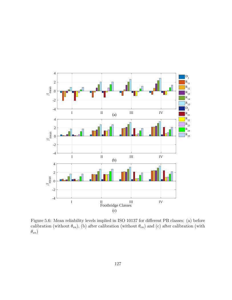
I II III IV-4

-2

0

2

4

βm

ean

I II III IVFootbridge Classes

-4

-2

0

2

4

βm

ean

I II III IV-4

-2

0

2

4

βm

ean

D1

R11

R12

R13

R14

R15

D2

R21

R22

R23

R24

R25

(a)

(b)

(c)

Figure 5.6: Mean reliability levels implied in ISO 10137 for different PB classes: (a) beforecalibration (without θen), (b) after calibration (without θen) and (c) after calibration (withθen)

127

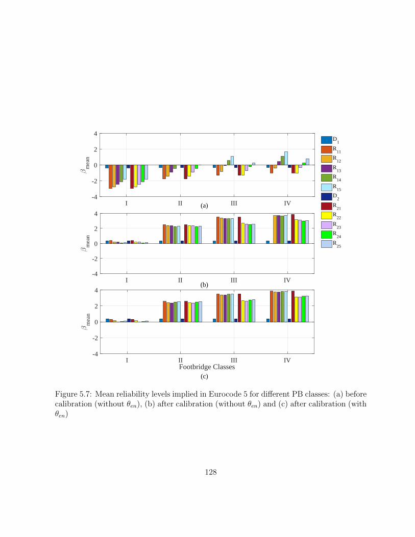
I II III IV-4

-2

0

2

4

βm

ean

D1

R11

R12

R13

R14

R15

D2

R21

R22

R23

R24

R25

I II III IV-4

-2

0

2

4

βm

ean


-4

-2

0

2

4

βm

ean

(a)

(c)

(b)

Figure 5.7: Mean reliability levels implied in Eurocode 5 for different PB classes: (a) beforecalibration (without θen), (b) after calibration (without θen) and (c) after calibration (withθen)

128

I II III IV-4

-2

0

2

4

βm

ean

D1

R11

R12

R13

R14

R15

D2

R21

R22

R23

R24

R25

I II III IV-4

-2

0

2

4

βm

ean


-4

-2

0

2

4

βm

ean

(c)

(b)

(a)

Figure 5.8: Mean reliability levels implied in British National Annex to Eurocode 1 (group)for different PB classes: (a) before calibration (without θen), (b) after calibration (withoutθen) and (c) after calibration (with θen)

129

I II III IV-4

-2

0

2

4

βm

ean

D1

R11

R12

R13

R14

R15

D2

R21

R22

R23

R24

R25

I II III IV-4

-2

0

2

4

βm

ean


-4

-2

0

2

4

βm

ean

(a)

(b)

(c)

Figure 5.9: Mean reliability levels implied in British National Annex to Eurocode 1 (crowd)for different PB classes: (a) before calibration (without θen), (b) after calibration (withoutθen) and (c) after calibration (with θen)

130

I II III IV-5

0

5

βm

ean

D1

R11

R12

R13

R14

R15

D2

R21

R22

R23

R24

R25

I II III IV-5

0

5

βm

ean


-5

0

5

βm

ean

(a)

(b)

(c)

Figure 5.10: Mean reliability levels implied in SETRA for different PB classes: (a) beforecalibration (without θen), (b) after calibration (without θen) and (c) after calibration (withθen)

131

1 2 3 4β

t

0

0.5

1

γa l

1 2 3 4β

t

0

0.5

1

γa l

0.050.100.150.20

1 2 3 4β

t

1

1.2

1.4

1.6

γG

1 2 3 4βt

1

1.5

2γ

G

1 2 3 4βt

1

1.2

1.4

1.6

γα

m

1 2 3 4β

t

1

1.5

2

2.5

γα

m(a) (b)

(d)

(e) (f)

(c)

m=1 m>1

Figure 5.11: Variation in partial factors with COV of limit acceleration for different targetreliability levels (βt) corresponding to (a) al (m=1), (b) al (m > 1), (c) G (m = 1), (d)G (m > 1), (e) αm (m = 1) and (f) αm (m > 1), where m is the resonating harmonic ofwalking frequency

132

0

0.5

1

1.5

2

2.5

βd

COV=0.05COV=0.10COV=0.15COV=0.20

ISO 10137 Eurocode 5 British National British National SÉTRA Annex (group) Annex (crowd)

Figure 5.12: Desired reliability by different guidelines for Class I of PBs in case of R15 fordifferent COVs of al

133

Chapter 6

Conclusions and recommendations

A comprehensive serviceability assessment of PBs under walking-induced excitations hasbeen undertaken in this dissertation under a controlled set of tests. The performance ofthe popular serviceability design provisions under single and groups of pedestrians hasbeen evaluated both in deterministic and probabilistic frameworks. This study has re-sulted in several recommendations to the existing guidelines in order to better align themwith experimental observations. This chapter highlights the significant contributions, keyconclusions, and recommendations for future work.

6.1 Significant contributions

The present research has led to several key contributions, which are summarized as follows:

1. A comprehensive experimental database of walking trials under different traffic sce-narios has been developed on three full-scale PBs with emphasis on bridges thatresonate with the higher harmonics of the walking frequency. This database is usefulfor verification of popular design load models and for effective comparison of theirperformances, which is especially important in order to improve the vibration service-ability design of PBs. Additionally, as the PBs are lively and the human-structureinteraction phenomena was observed, the database will significantly contribute to theinvestigation of such interaction phenomenon.

2. The capabilities of the design guidelines to reliably assess the serviceability perfor-mance of the three bridges considered in the study have been investigated. The large

134

discrepancies between the computed and measured responses point towards improv-ing the design provisions to produce reliable and economical designs.

3. Based on the study on the three bridges spanning a range of dynamic conditions,key recommendations have been proposed to reconcile the design guidelines throughdesign parameters, which already exist in the literature. The recommendations canbe easily incorporated into the existing design framework of the design methodologiesand thus could contribute towards the better design of PBs.

4. Although the uncertain nature of pedestrian-induced walking load has been well ac-knowledged and accounted for in the standards, uncertainties in the acceleration limitand structural properties have not been studied. Hence, a reliability-based evaluationhas been conducted for the design guidelines by incorporating uncertainties from allsources including the pedestrian and the structure. The current study is the firststudy to evaluate these guidelines in a reliability-based framework.

5. The results from the reliability analysis show that the guidelines fail to achieve suf-ficient reliability under rare traffic events, which could result in significant economiclosses. Hence, the guidelines have been calibrated in order to achieve acceptableperformance of the designs during rare traffic events, while at the same time pro-ducing economical designs. Assessing the guidelines in a reliability-based frameworkand subsequently calibrating them for improved design is a novel step towards theperformance-based design of PBs under the serviceability limit state.

6. Several peer-reviewed journal and conference articles have directly resulted from thiswork by the author.

6.2 Conclusions

Having highlighted the significant contributions, the key conclusions resulting from thisdissertation are summarized as follows:

1. One of the main conclusions of this study is that PBs that resonate with the higherharmonics of walking frequency, and not just the lowest harmonic, may be subjectedto excessive vibrations, thus leading to serviceability issues.

135

2. A comparison study between the measured and simulated responses under singlepedestrian walking tests for different scenarios of resonant and non-resonant condi-tions shows that the design walking load models are unable to capture the contri-butions from the transients, i.e. at the natural frequency of the structure for non-resonating cases (with respect to any of the harmonics), while they over-estimate forthe resonant cases where the natural frequency and the excitation frequency (or oneof the harmonics) overlap. For the case of resonance with a higher harmonic, thecontribution from the corresponding non-resonating harmonics are underestimatedby the models, which may be due to pedestrian-structure interaction. Moreover, fora fully non-resonant case (i.e. none of the harmonics are in resonance with the excita-tion), the models estimate the observations relatively well. These issues become veryimportant for aluminum PBs, which tend to exhibit natural frequencies outside whatis typically considered as the design frequency range, however tend to be lively dueto their low inherent damping and light weight. Hence, more sophisticated models,which address these shortcomings are needed to better estimate the serviceabilityperformance of such PBs.

3. The serviceability assessment under different crowd loads in accordance with the ex-isting design guidelines shows that the response in general is overestimated in thevertical direction and underestimated in the lateral direction. Key recommenda-tions are proposed in order to better align predictions through incorporating DLFsfrom more recent studies with higher number of harmonics, traffic-dependent walk-ing speed, appropriate harmonics for resonance, added mass from pedestrians, andappropriate multiplication factors. It is observed from the comparison study thatthe existing design methodologies can be improved substantially by adopting therecommendations proposed here.

4. The design provisions are also evaluated in terms of sufficiency and uniformity byconsidering all possible traffic situations expected during the design life of the struc-ture including design and rare traffic events. The reliability bounds, i.e., maximumand minimum reliability indices, reveal significant scatter over the range of designedconfigurations and classes of PBs. In terms of sufficiency, when a structure is de-signed for a specific crowd density (class), it does not satisfy the target value of 0(according to ISO 2934 for reversible failures) under the design traffic. However, theminimum reliability levels for all of the designs are close to 0. Classes I to III PBs,with low to dense design traffic levels, achieve very low reliability levels under heavytraffic corresponding to rare loading events. Hence, it is suggested that the guidelinesshould be calibrated for higher reliability at the design event in order to achieve suf-

136

ficient reliability during rare events. However, always designing for very dense trafficmay not be sound economically. Thus, it is recommended that comfort limits basedon the frequency of occurrence of traffic be adopted to achieve economical designsfor Class I to III bridges, while at the same time ensuring acceptable performanceduring rare loading events. Furthermore, design comfort limits should be establishedbased on bridge class to yield economic designs along with uniform reliability acrossthe classes.

5. A parametric study is performed to investigate the sensitivity of the reliability esti-mates to the uncertainties associated with a number of the key model variables. Thestudy shows that the uncertainties in the bridge moment of area and mass per unitlength have virtually no impact on the reliability estimates. On the other hand, theuncertainty in the elastic modulus has a significant contribution in the case of all ofthe design provisions except those in ISO 10137 for very low values of the responsereduction factors. On the other hand, the reliability results are not very sensitiveto the COV of damping. In general, all the variables corresponding to the structurecan conservatively be treated as deterministic for code calibration purposes. Thestudy also suggests that assuming a normal distribution for the limiting accelerationinstead of log-normal or an extreme value distribution will not have a significantimpact on the reliability estimates of the bridges.

6. A model error term is introduced in order to incorporate the recommendations inthe existing framework of the design provisions. Reliability analysis is carried outby introducing uncertainty in the model error term, which shows a positive impacton the reliability estimates, and hence this term can be assumed deterministic forcalibration purposes.

7. An attempt to calibrate the guidelines is made in the current thesis. The guidelinesachieve acceptable performance during the design as well as rare loading events aftercalibrating for a higher reliability at the design level. Moreover, adopting comfortlimits based on occurrence frequency of traffic and bridge class ensures economicdesigns through the calibrated design provisions. Similar to target reliability, a newterm called the desired reliability is introduced in the current study, which is requiredfor the calibration process. The desired reliability and corresponding partial factorsare estimated for all the guidelines. Although the partial factors are identical inall the guidelines for a given reliability index, the desired reliability is inconsistentacross the guidelines and subsequently the resulting partial factors for the calibrateddesign. It is also observed that estimates of the desired reliability and partial factorsare sensitive to the choice of COV for the acceleration limit. Hence, an appropriate

137

uncertainty model for acceleration limit is required in order to adopt the suitablepartial factors for the calibrated design procedures.

6.3 Limitations of the current study

After summarizing the key conclusions resulting from this dissertation, the limitations ofthe current study are outlined below:

• The current study adopts truss type metal PBs with simply supported boundaryconditions, idealized as a simply supported beam. Moreover, the structural responsehas been estimated in the modal domain with one dominating mode of vibration.Despite these assumptions, it is expected that the key observations will remain thesame in terms of the performance of the design load models in deterministic as wellas reliability-based frameworks, while the partial factors estimated in Chapter 5 arelimited to only metal PBs, for which the structural variables can be assumed deter-ministic. A sensitivity study should be performed with the uncertainty models of thestructural variables for different material characteristics and the assumption whetherthe structural variables can be assumed deterministic needs to be re-investigated forsuch cases.

• The key recommendations proposed in Chapter 5 to improve the design guidelines forserviceability assessment of PBs under crowd loads are based on observations fromonly a limited number of PBs. While most of the recommendations are expected tobe applicable to other bridges, the accuracy of the recommended multiplication anddynamic load factors should be investigated based on more experiments on differenttypes of bridges.

6.4 Recommendations for future study

There are several possible extensions to the present work to improve the serviceabilitydesign of PBs under walking-induced excitations, which are beyond the current scope ofstudy. These include:

1. The comprehensive database of walking tests developed in the current study canserve as a good test-bed for investigating human-structure interaction phenomenaobserved in many failures.

138

2. The current study is only limited to the performance of time-domain periodic loadmodels, which are adopted by the design guidelines. Recently, there is a trend towardsbiomechanical models. A performance verification for such load models could becarried out using this current database.

3. During the course of this experimental study, forces at the supports of the laboratorybridge specimens were also measured using load cells. The walking-induced forcemodels can be calibrated thorough these measured forces in the future, which cansubstantially contribute towards further improving the design guidelines.

4. The measured acceleration responses can be useful in order to estimate walking-induced forces through inverse analysis, which can substantially contribute towardsinvestigating the effect of human-structure interaction on the induced walking force.

5. The key recommendations proposed in the current study to improve the vibrationserviceability assessment of PBs under crowd loads are primarily based on exper-imental observations from two aluminum PBs. Additional bridge types and testscould add to the value and accuracy of the main conclusions from this work.

6. Based on the key recommendations proposed in the current study, a model error termhas been introduced to the existing design provisions. This term can be calibratedusing experimental observations on various PBs in the future.

7. The reliability analysis and corresponding code calibration is limited to the verticaldirection. The analysis can be easily extended to the lateral direction by adoptingdifferent configurations of PBs, which are more sensitive to the lateral vibrations andare within the lateral critical frequency ranges as suggested by the guidelines in Table2.3.

8. In the absence of a target reliability for calibration, the current study has iterativelyestimated the reliability level required for achieving sufficient reliability without con-ducting any cost-based analysis. In the future, a target reliability index can bedetermined using other measures such as consequence of failure.

139

References

AASHTHO LRFD. Guide specifications for the design of pedestrain bridges. AASHTHOLRFD Bridge Design, 2007.

M. Abu-Hilal and M. Mohsen. Vibration of beams with general boundary conditions dueto a moving harmonic load. Journal of Sound and Vibration, 232(4):703–717, 2000.

H. Adeli. Historic bridges: Evaluation, preservation, and management. CRC Press, 2016.

AIJES-V001. Guidelines for the evaluation of habitability to building vibration. Standard,Architectural Institute of Japan Recommendations, Tokyo, Japan, 2004.

D. E. Allen and T. M. Murray. Design criterion for vibrations due to walking. AISCJournal, 30(4):117–129, 1993.

P. Archbold, P. J. Fanning, and A. Pavic. Interactive horizontal load model for pedestrianscrossing footbridges. Bridge Structures, 1(3):169–176, 2005.

AS 5100. Bridge design, part 2: Design loads. Australian Standard, 2004.

H. Bachmann and W. Ammann. Vibrations in structures: induced by man and machines,volume 3. Iabse, 1987.

H. Bachmann, A. J. Pretlove, and H. Rainer. Dynamic forces from rhythmical human bodymotions. In: Vibration problems in structures: practical guidelines. Basel: Birkhauser,1995.

R. Bashor, T. Kijewski-Correa, and A. Kareem. On the wind-induced response of tallbuildings: the effect of uncertainties in dynamic properties and human comfort thresh-olds. In Proceedings of Americas Conference on Wind Engineering, Baton Rouge, LA,volume 31, 2005.

140

J. Blanchard, B. L. Davies, and J. W. Smith. Design criteria and analysis for dynamicloading of footbridges. In Proceeding of a Symposium on Dynamic Behaviour of Bridgesat the Transport and Road Research Laboratory, Crowthorne, Berkshire, England, May19, 1977, 1977.

M. Bocian, J. H. G. Macdonald, and J. F. Burn. Biomechanically inspired modellingof pedestrian-induced forces on laterally oscillating structures. Journal of Sound andVibration, 331(16):3914–3929, 2012.

M. Bocian, J. H. G. Macdonald, and J. F. Burn. Biomechanically inspired modeling ofpedestrian-induced vertical self-excited forces. Journal of Bridge Engineering, 18(12):1336–1346, 2013.

K. Breitung. Asymptotic approximations for multinormal integrals. Journal of EngineeringMechanics, 110(3):357–366, 1984.

J. M. W. Brownjohn, P. Fok, and P. Roche, M.and Moyo. Long span steel pedestrianbridge at singapore changi airport-part 1: Prediction of vibration serviceability problems.Structural Engineer, 82(16), 2004a.

J. M. W. Brownjohn, A. Pavic, and P. Omenzetter. A spectral density approach formodelling continuous vertical forces on pedestrian structures due to walking. CanadianJournal of Civil Engineering, 31(1):65–77, 2004b.

BS 5400. Steel concrete and composite bridges: Specification for loads; appendix c: Vibra-tion serviceability requirements for foot and cycle track bridges. UK: British StandardsAssociation, London, 1978.

C. Butz. Codes of practice for lively footbridges: State-of-the-art and required measures.Proceedings of footbridge, 2008.

C. H. Butz, C. H. Heinemeyer, A. Goldack, A. Keil, M. Lukic, E. Caetano, and A. Cunha.Advanced Load Models for Synchronous Pedestrian Excitation and Optimised DesignGuidelines for Steel Footbridges - SYNPEX). European Commission - Directorate-General for Research; EUR 23318; ISBN 978-92-79-08303-7, ISSN 1018-5593, 2008.

E. Caetano and A. Cunha. Dynamic tests on a lively footbridge. Proc., and Footbridge2002, pages 1–11, 2002.

E. Caetano, A. Cunha, F. Magalhaes, and C. Moutinho. Studies for controlling human-induced vibration of the pedro e ines footbridge, portugal. part 1: Assessment of dynamicbehaviour. Engineering Structures, 32(4):1069–1081, 2010.

141

CAN/CSA S6. Canadian highway bridge design code. Canadian Standards Association,Canada, 2011.

C. C. Caprani, J. Keogh, P. Archbold, and P. Fanning. Characteristic vertical response ofa footbridge due to crowd loading. 2011.

C. C. Caprani, J. Keogh, P. Archbold, and Fanning P. Enhancement factors for the verticalresponse of footbridges subjected to stochastic crowd loading. Computers & Structures,(102):87–96, 2012.

P. W. Chen and L. E. Robertson. Human perception thresholds of horizontal motion.Journal of the structural division, 92(8):1681–1695, 1972.

C. A. Cornell. A probability-based structural code. In Journal Proceedings, volume 66,pages 974–985, 1969.

Cornell University. Explaining why the millennium bridge wobbled, November 2005. URLhttps://www.sciencedaily.com/releases/2005/11/051103080801.htm.

A Cunha, E. Caetano, C. Moutinho, and F. Magalhaes. Damping identification in a stress-ribbon footbridge. Proceedings of EURODYN 2005, 2005.

Curbed New York. Squibb park bridge will cost $3.12m to fix once andfor all, October 2016. URL http://ny.curbed.com/2016/10/7/13201020/

squibb-park-bridge-brooklyn-construction-cost.

F. T. da Silva, H. M. B. F. Brito, and R. L. Pimentel. Modeling of crowd load in verticaldirection using biodynamic model for pedestrians crossing footbridges. Canadian Journalof Civil Engineering, 40(12):1196–1204, 2013.

P. Dallard, T. Fitzpatrick, A. Flint, et al. London millennium bridge: pedestrian-inducedlateral vibration. Journal of Bridge Engineering, 6(6):412–417, 2001.

F. Danbon and G. Grillaud. Dynamic behaviour of a steel footbridge: Characterization andmodelling of the dynamic loading induced by a moving crowd on the solferino footbridgein paris. Proceedings of Footbridge, 2005.

F. Dierick, M. Penta, D. Renaut, and C. Detrembleur. A force measuring treadmill inclinical gait analysis. Gait & posture, 20(3):299–303, 2004.

142

https://www.sciencedaily.com/releases/2005/11/051103080801.htm

http://ny.curbed.com/2016/10/7/13201020/squibb-park-bridge-brooklyn-construction-cost

http://ny.curbed.com/2016/10/7/13201020/squibb-park-bridge-brooklyn-construction-cost

A. Ebrahimpour, R. L. Sack, W. N. Patten, and A. Hamam. Experimental measurements ofdynamic loads imposed by moving crowds. In Structures Congress XII, pages 1385–1390,1994.

A. Ebrahimpour, A. Hamam, R. L. Sack, and W. N. Patten. Measuring and modelingdynamic loads imposed by moving crowds. Journal of Structural Engineering, 122(12):1468–1474, 1996.

H. Elftman. The measurement of the external force in walking. Science, 88(2276):152–153,1938.

B. R. Ellis. The influence of crowd size on floor vibrations induced by walking. StructuralEngineer, 81(6):20–27, 2003.

EN 1990. Eurocode - basis of structural design. European Committee of Standardization,Eurocode 0, 2001.

EN 1995-2. Design of timber structures - part 2: Bridges. European Committee of Stan-dardization, Eurocode 5, 2004.

FIB. Guidelines for the design of footbridges. Bulletin 32, Lausanne, 2005.

Y. Fujino, B. M. Pacheco, S. Nakamura, and P. Warnitchai. Synchronization of humanwalking observed during lateral vibration of a congested pedestrian bridge. Earthquakeengineering & structural dynamics, 22(9):741–758, 1993.

F. W. Galbraith and M. V. Barton. Ground loading from footsteps. The Journal of theAcoustical Society of America, 48(5B):1288–1292, 1970.

S. A. Gard, S. C. Miff, and A. D. Kuo. Comparison of kinematic and kinetic methodsfor computing the vertical motion of the body center of mass during walking. Humanmovement science, 22(6):597–610, 2004.

R. J. Hansen, J. W. Reed, and E. H. Vanmarcke. Human response to wind-induced motionof buildings. Journal of the structural division, 99(7):1589–1605, 1973.

F. C. Harper. The mechanics of walking. Research applied in Industry, 15(1):23–28, 1962.

A. M. Hasofer and N. C. Lind. Exact and invariant second-moment code format(for reliabil-ity analysis in multivariate problems). American Society of Civil Engineers, EngineeringMechanics Division, Journal, 100:111–121, 1974.

143

C. Heinemeyer, C. Butz, A. Keil, M. Schlaich, A. Golbeck, S. Trometor, M. Lukic,B. Chabrolin, A. Lemaire, P. Martin, A. Cunha, and E. Caetano. Design of lightweightfootbridges for human induced vibrations. EUR - Scientific and Technical Research Re-ports JRC53442, 2009. URL http://publications.jrc.ec.europa.eu/repository/

handle/JRC53442.

M. A. B. U. Hilal and H. S. Zibdeh. Vibration analysis of beams with general boundaryconditions traversed by a moving force. Journal of Sound and Vibration, 229(2):377–388,2000.

F. B. Hildebrand. Introduction to numerical analysis, section 9.4. New York: McGraw-Hill,1956.

HIVOSS. Design of footbridges. Human induced vibration of steel structures, 2008.

J. Humar. Dynamics of Structures. CRC press,, 2012.

A. W. Irwin. Human reactions to oscillations of buildings-acceptable limits. Build Inter-national, 8(2):7, 1975.

ISO 10137. Bases for design of structures - serviceability of buildings and walkways againstvibrations. Ethiopian Standards Agency, 2007.

ISO 2394. General principles on reliability for structures. Zurich: ISO, 1998.

J. Kanda, Y. Tamura, and K. Fujii. Probabilistic criteria for human perception of low-frequency horizontal motions. In Proceedings of symposium/workshop on serviceabilityof buildings, Ottawa, pages 260–269, 1988.

M. Kasperski and C. Sahnaci. Serviceability of pedestrian structures. In Proceedings ofthe 25th international modal analysis conference, Orlando, Florida, pages 774–98, 2007.

S. C. Kerr. Human Induced Loading on Staircases. PhD Thesis, Mechanical EngineeringDepartment, University College London, UK, 1998.

S. Kim, K. Cho, M. Choi, M. S. Choi, and J. Y. Lim. Development of human body modelfor the dynamic analysis of footbridges under pedestrian induced excitation. Journal ofSteel Structures, 8:333–345, 2008.

H. Kramer and H. W. Kebe. Man-induced structural vibrations. Der Bauingenieur, 54(5):195–199, 1980.

144

http://publications.jrc.ec.europa.eu/repository/handle/JRC53442

http://publications.jrc.ec.europa.eu/repository/handle/JRC53442

J. H. G. Macdonald. Pedestrian-induced vibrations of the clifton suspension bridge, uk.Proceedings of the ICE-Bridge Engineering, 161(2):69–77, 2008.

W. Mader and A. Pieper. Schwansbell bridge celebrating 50th birthday. Structural engi-neering international, 16(4):356–359, 2006.

Y. Matsumoto, T. Nishioka, H. Shiojiri, and K. Matsuzaki. Dynamic design of footbridges.In IABSE proceedings, volume 2, 1978.

NA to BS EN 1991-2. UK national annex to Eurocode 1. actions on structures-part 2:Traffic loads on bridges. British Standards Institution, 2003.

S. Nakamura. Field measurements of lateral vibration on a pedestrian suspension bridge.Structural Engineer, 81(22), 2003.

A. S. Nowak and K. R. Collins. Reliability of structures. CRC Press, 2012.

A. Pachi and T. Ji. Frequency and velocity of people walking. Structural Engineer, 83(3),2005.

L. Pedersen. Damping effect of humans. In Topics on the Dynamics of Civil Structures,Volume 1, pages 1–6. Springer, 2012.

L. Pedersen and C. Frier. Sensitivity of footbridge vibrations to stochastic walking param-eters. Journal of Sound and Vibration, 329(13):2683–2701, 2010.

G. Pernica. Dynamic load factors for pedestrian movements and rhythmic exercises. Cana-dian Acoustics, 18(2):3, 1990.

J. Perry. Gait analysis. Normal and pathological function, 1, 1992.

R. L. Pimentel. Vibrational performance of pedestrian bridges due to human-induced loads.PhD thesis, University of Sheffield, 1997.

K. Portier, T. J. Keith, and S. M. Roberts. Body weight distributions for risk assessment.Risk analysis, 27(1):11–26, 2007.

J. W. Qin, S. S. Law, Q. S. Yang, and N. Yang. Pedestrian–bridge dynamic interaction,including human participation. Journal of Sound and Vibration, 332(4):1107–1124, 2013.

V. Racic and J. M. W. Brownjohn. Stochastic model of near-periodic vertical loads due tohumans walking. Advanced Engineering Informatics, 25(2):259–275, 2011.

145

V. Racic, J. M. W. Brownjohn, and A. Pavic. Human walking and running forces: Novelexperimental characterization and application in civil engineering dynamics. In Proceed-ings IMAC XXVI Conference, Orlando/Florida/USA, 2008.

R. Rackwitz and B. Flessler. Structural reliability under combined random load sequences.Computers & Structures, 9(5):489–494, 1978.

M. D. Rahman and K. Yu. Total least squares approach for frequency estimation usinglinear prediction. Acoustics, Speech and Signal Processing, IEEE Transactions on, 35(10):1440–1454, 1987.

J. H. Rainer, G. Pernica, and D. E. Allen. Dynamic loading and response of footbridges.Canadian Journal of Civil Engineering, 15(1):66–71, 1988.

E. Reynders, K. Maes, G. Lombaert, and G. De Roeck. Uncertainty quantification inoperational modal analysis with stochastic subspace identification: Validation and ap-plications. Mechanical Systems and Signal Processing, 66:13–30, 2016.

F. Ricciardelli and A. D. Pizzimenti. Lateral walking-induced forces on footbridges. Journalof bridge engineering, 12(6):677–688, 2007.

P. O. Riley, G. Paolini, U. Della Croce, K. W. Paylo, and D. C. Kerrigan. A kinematicand kinetic comparison of overground and treadmill walking in healthy subjects. Gait& posture, 26(1):17–24, 2007.

I. Roos. Human induced vibrations of footbridges: Application and comparison of pedes-trian load model. Master’s thesis, Delft University of Technology, Netherlands, 2009.

C. Sahnaci and M. Kasperski. Random loads induced by walking. In Proceedings of thesixth European conference on structural dynamics, volume 1, pages 441–6, 2005.

R. Salgado, J. M. Branco, P. J. S. Cruz, and G. Ayala. Serviceability assessment of thegois footbridge using vibration monitoring. Case Studies in Nondestructive Testing andEvaluation, 2:71–76, 2014.

W. W. Sanders and R. E. Abendroth. Construction and evaluation of a continuous alu-minum girder highway bridge. American Welding Society(USA), pages 107–114, 1995.

H. Schulze. Dynamic effects of the live load on footbridges. Signal und Schiene, 24(2):91–93, 1980.

146

SETRA. Assessment of vibrational behaviour of footbridges under pedestrian loading.Technical guide SETRA, Paris, France, 2006.

F. T. Silva and R. L. Pimentel. Biodynamic walking model for vibration serviceability offootbridges in vertical direction. In Proceeding of the 8th International Conference onStructural Dynamics (Eurodyn 2011), pages 1090–1096, 2011.

G. G. Simoneau. Kinesiology of walking. Kinesiology of the musculoskeletal system: foun-dations for physical rehabilitation, 1:523, 2002.

T. Siwowski. Aluminium bridges–past, present and future. Structural engineering inter-national, 16(4):286–293, 2006.

M. G. Stewart. Optimization of serviceability load combinations for structural steel beamdesign. Structural Safety, 18(2):225–238, 1996.

A. Sychterz. Vibration characterisation of aluminium pedestrian bridges. 2014.

A. Sychterz, A. Sadhu, S. Narasimhan, and S. Walbridge. Results from modal testing ofthe daigneault creek bridge. In CSCE 2013 General Conference, Montral, Qubec, May29 to June 1, 2013.

T. Tredgold. Elementary principles of carpentry. E. & FN Spon, 1890.

K. Van Nimmen, G. Lombaert, G. De Roeck, and P. Van den Broeck. Vibration serviceabil-ity of footbridges: Evaluation of the current codes of practice. Engineering Structures,59:448–461, 2014.

A. C. W. M. Vrouwenvelder and A. J. M. Siemes. Probabilistic calibration procedure forthe derivation of partial safety factors for the netherlands building codes. HERON, 32(4), 1987, 1987.

J. E. Wheeler. Prediction and control of pedestrian-induced vibration in footbridges. Jour-nal of the structural division, 108(ST-9), 1982.

M. W. Whittle. Gait analysis: an introduction. 2003.

M. Willford. Dynamic actions and reactions of pedestrians. In Proceedings of the Interna-tional Conference on the Design and Dynamic Behaviour of Footbridges, Paris, France,November 20-22, pages 66–74, 2002.

147

M. R. Willford, P. Young, and M. CEng. A design guide for footfall induced vibration ofstructures. Concrete Society London, UK, 2006. ISBN 9781904482291.

M. Yamasaki, T. Sasaki, and M. Torii. Sex difference in the pattern of lower limb move-ment during treadmill walking. European journal of applied physiology and occupationalphysiology, 62(2):99–103, 1991.

P. Young. Improved floor vibration prediction methodologies. In Proceedings Arup’s Sem-inar on Structural Vibration and Structure-Borne Noise: Current Developments in As-sessment and Design, 4 October 2001, ImechE, London, 2001.

F. Zheng, L. Shao, V. Racic, and J. Brownjohn. Measuring human-induced vibrations ofcivil engineering structures via vision-based motion tracking. Measurement, 83:44–56,2016.

S. Zivanovic. Probability-based estimation of vibration for pedestrian structures due towalking. PhD thesis, University of Sheffield, 2006.

S. Zivanovic. Benchmark footbridge for vibration serviceability assessment under the verti-cal component of pedestrian load. Journal of Structural Engineering, 138(10):1193–1202,2012.

S. Zivanovic, A. Pavic, and P. Reynolds. Vibration serviceability of footbridges underhuman-induced excitation: a literature review. Journal of sound and vibration, 279(1):1–74, 2005.

S. Zivanovic, A. Pavic, and P. Reynolds. Probability-based prediction of multi-mode vi-bration response to walking excitation. Engineering Structures, 29(6):942–954, 2007.

S. Zivanovic, A. Pavic, and E. T. Ingolfsson. Modeling spatially unrestricted pedestriantraffic on footbridges. Journal of Structural Engineering, 136(10):1296–1308, 2010.

148

APPENDICES

149

Appendix A

Response simulation

The analytical solution for Equation 2.24 are derived, based on the works by Abu-Hilaland Mohsen (2000) and Hilal and Zibdeh (2000), through employing the principle of su-perposition of responses from a constant moving load G and the harmonic loading terms.The displacement response Xn under a constant moving load P (t) = G as shown in Figure2.12 is given by (Hilal and Zibdeh, 2000):

Xn =G exp(−ζnωnt)(Yn1 + exp(ζnωnt)Yn2)L

ωdnMn((ζnωnL)4 + 2(ζnωnL2ωdn)2 + 2(ζnωnLvπ)2 + (ωdnL)4 − 2(ωdnLvπ)2 + (vπ)4)(A.1)

with,

Yn1 = (vπζ2nω

2nL

2 + v3π3 − ω2dnL

2vπ) sin(ωdnt) + 2ζnωnL2ωdnvπ cos(ωdnt)

Yn2 = (−Lωdnv2π2 + L3ωdnζ2nω

2n + L3ω3

dn) sin(vπt

L)− 2L2ωdnζnωnvπ cos(vπt/L)

(A.2)

where, ωdn = ωn√

1− ζ2n with ωn and ζn being the nth natural frequency and damping

constant of the structure.

The displacement response due to the sinusoidal moving force P (t) = Gαm sin(m2πfs)for mth harmonic can be derived as (Abu-Hilal and Mohsen, 2000):

Xmn = F2(t1 + t2 + t3 + t4 + t5 + t6 + t7 + t8 + t9 + t10) (A.3)

150

where, the terms, t1 · · · t10, F2, are given by:

F2 =Gαmn

4Mnωdn

t1 = −(q3

q4

+q9

q10

) cos((vπ

L+ ωm)t)

t2 = (q5

q6

+q7

q8

) cos((vπ

L− ωm)t)

t3 = −(ζnωnq4

− ζnωnq10

) sin((vπ

L+ ωm)t)

t4 = (ζnωnq6

− ζnωnq8

) sin((vπ

L− ωm)t)

t5 = −(q1q3

q13

− q1q3

q14

) exp(tvπ

L) cos(ωmt)

t6 = (q2q4

q15

− q2q4

q16

) exp(−tvπL

) cos(ωmt)

t7 = (q3q11

q13

+q3q12

q14

) exp(tvπ

L) sin(ωmt)

t8 = −(q4q11

q15

+q4q12

q16

) exp(−tvπL

) sin(ωmt)

t9 = (q3

q4

− q5

q6

− q7

q8

+q9

q10

+q1q3

q13

− q1q3

q14

− q2q4

q15

+q2q4

q16

) exp(−tζnωn) cos(ωdnt)

t10 = (ζnωnq4

− ζnωnq6

− ζnωnq8

+ζnωnq10

− q3q11

q13

+q3q12

q14

+q4q11

q15

− q4q12

q16

) exp(−tζnωn) sin(ωdnt)

Here, ωm equals to m2πfs for the mth harmonic and the terms qi, i = 1, 2...16 are defined

151

as follows:

q1 = ζnωn +vπ

L; q2 = ζnωn −

vπ

L; q3 = ωdn −

vπ

L− ωm

q4 = (ζnωn)2 + (ωdn −vπ

L− ωm)2; q5 = ωdn −

vπ

L+ ωm

q6 = (ζnωn)2 + (ωdn −vπ

L+ ωm)2; q7 = ωdn +

vπ

L− ωm

q8 = (ζnωn)2 + (ωdn +vπ

L− ωm)2; q9 = ωdn +

vπ

L+ ωm

q10 = (ζnωn)2 + (ωdn +vπ

L+ ωm)2; q11 = ωdn − ωm

q12 = ωdn + ωm; q13 = (ζnωn +vπ

L)2 + (ωdn − ωm)2

q14 = (ζnωn +vπ

L)2 + (ωdn + ωm)2; q15 = (ζnωn −

vπ

L)2 + (ωdn − ωm)2

q16 = (ζnωn −vπ

L)2 + (ωdn + ωm)2

The total displacement response for mode n can be written as the sum of the static anddynamic parts contributed by m harmonics of the excitation force as follows:

Yn = Xn +m∑i=1

Xmn (A.4)

152

Appendix B

Mode shapes from finite elementmodels

The first vertical and lateral mode shapes of the three full scale pedestrian bridges fromthe finite element models are shown in Figures B.1 to B.5.

Figure B.1: First lateral mode at 2.3 Hz for the 12.2 m bridge specimen

153

Figure B.2: First vertical mode at 13.0 Hz for the 12.2 m bridge specimen

Figure B.3: First lateral mode at 1.0 Hz for the 22.9 m bridge specimen

Figure B.4: First vertical mode at 4.4 Hz for the 22.9 m bridge specimen

154

Figure B.5: First vertical mode at 3.40 Hz for the Daigneault Creek bridge specimen (takenfrom Sychterz et al. (2013))

155

Appendix C

Modal identification through freevibration tests

The free vibration tests performed in the current study for identification of modal frequencyand damping ratios involve measurement of the bridge acceleration after the applicationof an impulse through hammer (in vertical direction) or imposed displacement (in lateraldirection). The modal identification methodologies adopted in this thesis are discussed inthe following section:

C.1 Fast Fourier Transform or FFT method

The Fast Fourier Transform or FFT method is the simplest form of modal analysis in orderto estimate the modal frequency of a structure. A Fast Fourier Transform is performedon the time-series data collected on the bridge during the modal testing such as impactloading test. Since these tests only apply an impact without any frequency from theexcitation on the structure, peaks in the FFT from these free vibration response of thestructures correspond to the natural frequencies of the structure. Figure 3.5 show samplevertical acceleration time histories and corresponding FFT plots of the 22.9 m laboratoryspecimens during hammer tests on the bridge. The first three vertical natural frequenciesare shown in the FFT plots through picking the peaks of the FFT amplitudes.

156

2 4 6 8 10 12Time (Sec)

-0.04

-0.02

0

0.02

0.04

Acc

elea

rtio

n (m

/s2 ) Data

exponential fit

2 2.5 3 3.5 4Time (Sec)

-0.03

-0.02

-0.01

0

0.01

0.02

(b)

u(t) = ae -2πfnζ

nt

(a)

at1

at2

at3

at4

Figure C.1: (a) Exponential envelop fitted to first vertical modal acceleration time historyand (b) illustration of decaying time history with successive peaks, measured at the midspan of the 22.9 m bridge specimen during hammer test

C.2 Modal damping estimation

The current study employs the simple free vibration decay method to estimate the damping.As the decays measured after application of the impact force should contain only thecontribution of a single mode, the mode of interests are isolated through applying band-pass filters. Figure C.1 (a) shows the acceleration data from the 22.9 m bridge specimencorresponding to the natural frequency of 4.58 Hz. The exponential decay method isapplied to the filtered data in order to estimate the damping ratio corresponding to thatmode. The most common methods of acquiring damping ratio from free vibration decaydata are the exponential envelope and log-decrement methods.

In the exponential envelope method, an exponential curve is fitted to the peaks of thefiltered acceleration time history as shown Figure Figure C.1 (a). The fitted curve is inthe form of u(t) = ae−2πfnζnt, from which the damping ratio ζn can be estimated withknown value of structural frequency fn. On the other hand, in log-decrement method, thesuccessive peaks are obtained from the decaying time-history trace, for example, at1 , at2 ,at3 and at4 , in Figure C.1 (b) at respectively times t1, t2, t3 and t4. The damping ratio canbe determined as (Humar, 2012):

ζn =1

2πlnat1 − at2at3 − at4

(C.1)

In the current study both the methods of estimating damping ratio is employed. As

157

negligible deviations were observed between the two methods, only the damping valuesobtained using logarithmic decrement are reported in Table 3.7.

158

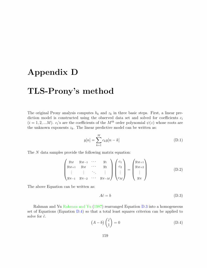
Appendix D

TLS-Prony’s method

The original Prony analysis computes hk and zk in three basic steps. First, a linear pre-diction model is constructed using the observed data set and solved for coefficients ci(i = 1, 2, ...M). ci’s are the coefficients of the M th order polynomial ψ(z) whose roots arethe unknown exponents zk. The linear predictive model can be written as:

y[n] =M∑k=1

cky[n− k] (D.1)

The N data samples provide the following matrix equation:yM yM−1 · · · y1

yM+1 yM · · · y2...

.... . .

...yN−1 yN−2 · · · yN−M

c1

c2...cM

=

yM+1

yM+2...yN

(D.2)

The above Equation can be written as:

Ac = b (D.3)

Rahman and Yu Rahman and Yu (1987) rearranged Equation D.3 into a homogeneousset of Equations (Equation D.4) so that a total least squares criterion can be applied tosolve for c. (

A− b)(c

1

)= 0 (D.4)

159

This can be written as:Dd = 0 (D.5)

The rank L of matrix D′, which minimizes ||D′ −D||F , is determined. The solution for dcan be estimated using:

d =1

α

β∑i=L+1

v∗i,M+1Vi (D.6)

where:

β = rank(B); α =

β∑i=L+1

|vi,M+1|2 (D.7)

In Equation D.6, vij is the jth element of Vi. σi, Ui and Vi are the ith singular values, leftand right singular vectors, respectively, obtained through singular value decomposition ofthe matrix D.

D′ =L∑i=1

σiUiVHi (D.8)

The first M values of d constitute the estimated vector c.

After obtaining the solution for c, the zeros of the following polynomial ψ(z) are solvedwhose roots are the unknown exponents zk:

ψ(z) = zM + c1zM−1 + · · ·+ cM (D.9)

Now, the unknown values of hk are obtained by solving the linear Equations in EquationD.10 and subsequently the amplitudes Ak corresponding to the frequencies of interest areextracted.

z01 z0

2 · · · z0M

z11 z1

2 · · · z1M

......

. . ....

zM−11 zM−1

2 · · · zM−1M

h1

h2...hM

=

y[1]y[2]

...y[M ]

(D.10)

160

Evaluation and Calibration of Pedestrian Bridge Standards ...

Documents

Transcript of Evaluation and Calibration of Pedestrian Bridge Standards ...