Evaluating the Capabilities of the Lattice Boltzmann Method...

EVALUATING THE CAPABILITIES OF THE

LATTICE BOLTZMANN METHOD FOR

NON-NEWTONIAN AND FREE-SURFACE FLOW

TOWARDS APPLICATIONS IN WELLBORE

CEMENTING

by

Matthew Grasinger

BS in Civil Engineering, University of Pittsburgh, Pittsburgh, PA

2013

Submitted to the Graduate Faculty of

the Swanson School of Engineering in partial fulfillment

of the requirements for the degree of

Master of Science

University of Pittsburgh

2016

UNIVERSITY OF PITTSBURGH

SWANSON SCHOOL OF ENGINEERING

This thesis was presented

by

Matthew Grasinger

It was defended on

July 21, 2016

and approved by

John C. Brigham, PhD, Associate Professor, Department of Civil and Environmental

Engineering

Julie M. Vandenbossche, PhD, Associate Professor, Department of Civil and

Environmental Engineering

Anthony T. Iannacchione, PhD, Associate Professor, Department of Civil and


Thesis Advisor: John C. Brigham, PhD, Associate Professor, Department of Civil and


ii

Copyright c© by Matthew Grasinger

2016

iii

EVALUATING THE CAPABILITIES OF THE LATTICE BOLTZMANN

METHOD FOR NON-NEWTONIAN AND FREE-SURFACE FLOW

TOWARDS APPLICATIONS IN WELLBORE CEMENTING

Matthew Grasinger, M.S.

University of Pittsburgh, 2016

When oil and gas wellbores are drilled, barriers must be put in place to ensure that fluids

do not leak out of the wellbore. Wellbore leakage can lead to environmental damage, loss of

pressure at the wellhead, and consequently, loss of production. An important yet vulnera-

ble barrier is the cement annulus. Every well has unique subsurface conditions, and so no

cement slurry mix design both performs well and is economical for cementing all wells. The

lattice Boltzmann method (LBM) is a promising technique for simulating primary wellbore

cementing because it is well-suited for efficiently simulating non-Newtonian flows, multi-

phase multicomponent flows, and flows through complex geometries–namely, some of the

complexities associated with the mechanics of primary cementing.

Despite the advantages of LBM, there are considerations that must be made, as with

all computational methods, in regards to the accuracy and numerical stability of the so-

lution. Issues with accuracy and numerical stability are especially relevant in the flow of

non-Newtonian fluids because of the nonlinear constitutive relationship between shear stress

and strain-rate. Chapter 1 is a numerical investigation of the accuracy, stability, and com-

putational efficiency of different LB methods in simulating non-Newtonian fluid flow. The

accuracy and computational time are presented in Section 1.4 for various LB methods applied

to two different benchmark problems, Poiseuille flow and lid-driven cavity flow, with two dif-

ferent non-Newtonian constitutive models, the Bingham plastic constitutive relationship and

a power-law constitutive relationship.

iv

Once the ground-work has been laid for simulating non-Newtonian flows using LBM, the

algorithm was extended in Chapter 2 to incorporate simulation of free-surface flow. The ex-

tended LBM model was used to study primary cementing of a dry annulus, i.e. an annulus

that is not filled with drilling mud. More specifically, the study involved defining differ-

ent cement slurry flows and investigating how well each slurry flow filled different wellbore

geometries. The study is followed by conclusions and a discussion of future work.

v

TABLE OF CONTENTS

PREFACE . . . . . . . . . . . . . . . . . . . . . . . . . . . . . . . . . . . . . . . . . xi

1.0 NUMERICAL INVESTIGATION OF THE ACCURACY, STABIL-

ITY, AND EFFICIENCY OF LATTICE BOLTZMANN MODELS IN

SIMULATING NON-NEWTONIAN FLUID FLOW . . . . . . . . . . . 1

1.1 Abstract . . . . . . . . . . . . . . . . . . . . . . . . . . . . . . . . . . . . . . 1

1.2 Introduction . . . . . . . . . . . . . . . . . . . . . . . . . . . . . . . . . . . 2

1.3 Lattice Boltzmann Method for Simulation of Non-Newtonian Fluids . . . . . 7

1.3.1 The Boltzmann Equation . . . . . . . . . . . . . . . . . . . . . . . . . 8

1.3.2 Collision Operator . . . . . . . . . . . . . . . . . . . . . . . . . . . . . 9

1.3.2.1 Bhatnagar-Gross-Krook (BGK) . . . . . . . . . . . . . . . . . 9

1.3.2.2 Multiple-relaxation Time (MRT) . . . . . . . . . . . . . . . . 14

1.3.3 Stability Enhancement through Artificial Dissipation: Entropic Filtering 16

1.3.4 Boundary Conditions . . . . . . . . . . . . . . . . . . . . . . . . . . . 19

1.3.5 Applied Forces . . . . . . . . . . . . . . . . . . . . . . . . . . . . . . . 20

1.3.6 Strain-rate Tensor . . . . . . . . . . . . . . . . . . . . . . . . . . . . . 20

1.3.7 Non-Newtonian Constitutive Equations . . . . . . . . . . . . . . . . . 21

1.3.7.1 Bingham Plastic . . . . . . . . . . . . . . . . . . . . . . . . . 21

1.3.7.2 Power-law . . . . . . . . . . . . . . . . . . . . . . . . . . . . . 21

1.4 Numerical Study . . . . . . . . . . . . . . . . . . . . . . . . . . . . . . . . . 22

1.4.1 Poiseuille Flow . . . . . . . . . . . . . . . . . . . . . . . . . . . . . . . 22

1.4.1.1 Bingham Plastic Fluids . . . . . . . . . . . . . . . . . . . . . . 24

1.4.1.2 Power-law Fluids . . . . . . . . . . . . . . . . . . . . . . . . . 35

vi

1.4.2 Lid-driven Cavity Flow . . . . . . . . . . . . . . . . . . . . . . . . . . 39

1.4.2.1 Bingham Plastic Fluids . . . . . . . . . . . . . . . . . . . . . . 41

1.4.2.2 Power-law Fluids . . . . . . . . . . . . . . . . . . . . . . . . . 45

1.5 Conclusions . . . . . . . . . . . . . . . . . . . . . . . . . . . . . . . . . . . . 48

2.0 FREE SURFACE ANDNON-NEWTONIAN SIMULATION OFWELL-

BORE CEMENTING USING THE LATTICE BOLTZMANNMETHOD 50

2.1 Abstract . . . . . . . . . . . . . . . . . . . . . . . . . . . . . . . . . . . . . . 50

2.2 Introduction . . . . . . . . . . . . . . . . . . . . . . . . . . . . . . . . . . . 51

2.3 Numerical Methods . . . . . . . . . . . . . . . . . . . . . . . . . . . . . . . 54

2.3.1 Lattice Boltzmann Method . . . . . . . . . . . . . . . . . . . . . . . . 54

2.3.2 Cement Slurry Constitutive Relationship . . . . . . . . . . . . . . . . 55

2.3.3 Free Surface Flow . . . . . . . . . . . . . . . . . . . . . . . . . . . . . 55

2.3.4 Capturing the Free-Surface . . . . . . . . . . . . . . . . . . . . . . . . 56

2.3.4.1 Mass Transfer . . . . . . . . . . . . . . . . . . . . . . . . . . . 56

2.3.4.2 Cell States . . . . . . . . . . . . . . . . . . . . . . . . . . . . . 57

2.3.4.3 Updating Cell States and Mass Redistribution . . . . . . . . . 58

2.3.5 Boundary Conditions at the Free-Surface . . . . . . . . . . . . . . . . 63

2.3.6 Resulting Algorithm for Simulating Free-Surface Flow using the Lattice

Boltzmann Method . . . . . . . . . . . . . . . . . . . . . . . . . . . . 65

2.4 Numerical Study of Primary Cementing . . . . . . . . . . . . . . . . . . . . 65

2.5 Conclusions . . . . . . . . . . . . . . . . . . . . . . . . . . . . . . . . . . . . 71

3.0 CONCLUSIONS . . . . . . . . . . . . . . . . . . . . . . . . . . . . . . . . . . 73

BIBLIOGRAPHY . . . . . . . . . . . . . . . . . . . . . . . . . . . . . . . . . . . . 75

vii

LIST OF TABLES

1.1 Bingham plastic Poiseuille flow . . . . . . . . . . . . . . . . . . . . . . . . . . 25

1.2 Power-law Poiseuille flow . . . . . . . . . . . . . . . . . . . . . . . . . . . . . 38

1.3 Bingham plastic, lid-driven cavity flow; Bn = 1. . . . . . . . . . . . . . . . . 42

1.4 Bingham plastic, lid-driven cavity flow; Bn = 10. . . . . . . . . . . . . . . . . 43

1.5 Bingham plastic, lid-driven cavity flow; Bn = 100. . . . . . . . . . . . . . . . 44

1.6 Power-law, lid-driven cavity flow; n = 0.5. . . . . . . . . . . . . . . . . . . . . 46

1.7 Power-law, lid-driven cavity flow; n = 1.5. . . . . . . . . . . . . . . . . . . . . 47

2.1 Cell state transition rules. . . . . . . . . . . . . . . . . . . . . . . . . . . . . 58

viii

LIST OF FIGURES

1.1 Schematic of D2Q9 lattice, each node is connected to its neighbor by one of

eight discrete velocity vectors . . . . . . . . . . . . . . . . . . . . . . . . . . . 10

1.2 Example of oscillations that can occur as a result of overrelaxation; the collision

frequency, ω = 1.95 and µapp ≈ 0.0043 . . . . . . . . . . . . . . . . . . . . . . 13

1.3 Schematic of Poiseuille flow; no-slip boundary conditions are enforced at the

top and bottom boundaries, and periodic boundary conditions are enforced at

the left and right boundaries. The size of the domain is L = 32 and H = 64. 23

1.4 LBM approximation using BGK and m = 105 compared to the analytical

solution for τy = 16× 10−5. . . . . . . . . . . . . . . . . . . . . . . . . . . . . 27

1.5 LBM approximation using BGK and m = 108 compared to the analytical

solution for τy = 16× 10−5. . . . . . . . . . . . . . . . . . . . . . . . . . . . . 28

1.6 Particle distributions in the 5 direction (left) and 8 direction (right) compared

to their respective quasiequilibriums. The top two plots are for the BGK with

m = 105, the bottom two are for the BGK with m = 108. . . . . . . . . . . . 30

1.7 Particle distributions in the 5 direction (left) and 8 direction (right) compared

to their respective quasiequilibriums for the MRT with m = 108. . . . . . . . 31

1.8 Evolution of relative L2 norm, εneq with time. The norm of the εneq across the

height of the channel is an indicator of an increase in oscillations at the lattice

level due to the ε moment. . . . . . . . . . . . . . . . . . . . . . . . . . . . . 33

1.9 Evolution of relative L2 norm, qxneq with time. The norm of the qneq

x across

the height of the channel is an indicator of an increase in oscillations at the

lattice level due to the qx moment. . . . . . . . . . . . . . . . . . . . . . . . . 34

ix

1.10 Cumulative relative L2 norm, εneq with time. Oscillations can have a positive

effect on each other, building up. The cumulative relative L2, εneq is a measure

of how much oscillations due to the ε moment may have been building in time. 36

1.11 Cumulative relative L2 norm, qneqx with time. Oscillations can have a positive

effect on each other, building up. The cumulative relative L2, qneqx is a measure

of how much oscillations due to the qx moment may have been building in time. 37

1.12 Schematic of lid-driven cavity flow; a velocity is prescribed tangential to the

top boundary and no-slip is enforced at the remaining boundaries. L = 100 . 40

2.1 Example of cell state transitions. The interface cell highlighted in red on the

left is transitioned to a gas cell as it has emptied. On the right, the three cells

highlighted in red were transitioned from fluid to interface cells in order to

keep the interface continuous. . . . . . . . . . . . . . . . . . . . . . . . . . . 62

2.2 Example of a scenario in which particle distributions are missing post-streaming. 64

2.3 Particle distributions at free-surface for a pair of opposing lattice directions

after gas pressure, ρG, is in the particle distribution form. . . . . . . . . . . . 65

2.4 Example simulation used in primary cementing study. The black rectangles

on the left boundary represent notches protruding from the rock formation

surface. The contours are of the primary fluid (cement slurry) mass. The

schematic on the right is courtesy of [1] . . . . . . . . . . . . . . . . . . . . . 67

2.5 Wellbore geometries considered in the study. . . . . . . . . . . . . . . . . . . 69

2.6 Percent of voids in wellbore at the end of simulation for each cement slurry

flow through each wellbore geometry. . . . . . . . . . . . . . . . . . . . . . . 70

x

PREFACE

I would like to thank my wife and best friend, Shelby, my parents, and my family. Their

love, support, and example means everything to me. I would like to thank the best advisor

ever, Dr. John Brigham, for his patience and for all that he has taught me. I would also like

to thank the other members of my committee, Dr. Julie Vandenbossche, and Dr. Anthony

Iannacchione, both of whom have been great guides and teachers to me. Lastly, I would like

to thank my fellow students, especially Rob, Jing, Mo, and Scott, for helping me to learn

along the way and for the comradery that every graduate student needs.

xi

1.0 NUMERICAL INVESTIGATION OF THE ACCURACY, STABILITY,

AND EFFICIENCY OF LATTICE BOLTZMANN MODELS IN

SIMULATING NON-NEWTONIAN FLUID FLOW

1.1 ABSTRACT

The Lattice Boltzmann method (LBM) is a method based on computational statistical me-

chanics that is well-suited for complex flow such as non-Newtonian, free surface, and mul-

tiphase multicomponent flow. Non-Newtonian flow is the primary focus of this Chapter, as

many practical engineering problems such as the flow of cement slurry and concrete, the

filling of molds by molten metals and plastics, blood flow, etc., are best modeled as non-

Newtonian fluids. LBM is typically applied to simulate flow through a series of time seps,

each consisting of streaming particle distributions to neighboring nodes, and collisions of

particle distributions at each node through a collision operator. The collision operator is of

interest because it, along with the equilibrium distribution function, determine the physics

that are simulated, e.g. constitutive laws, interfacial dynamics, etc., and it has implications

on numerical stability and computational efficiency. In this Chapter, various collision opera-

tors and methods for stability enhancement were examined for their suitability for simulating

non-Newtonian fluid flows in terms of accuracy, numerical stability and computational effi-

ciency. The investigation was carried out as a numerical study looking for qualitative, yet

practical, results; it included testing the BGK and MRT collision operators, with and with-

out entropic filtering, as applied to Bingham plastics and power-law fluids. Two different

benchmark problems were chosen for the flows: Poiseuille flow, and lid-driven square cavity

flow. The test results are followed by recommendations for choice collision scheme given

priority and problem type.

1

1.2 INTRODUCTION

The dynamic viscosity of a fluid is a measure of its resistance to shear deformation. For

many fluids, at a constant temperature, the dynamic viscosity can be considered as con-

stant. These fluids are known as Newtonian fluids. Non-Newtonian fluids have an apparent

dynamic viscosity, or apparent resistance to shear stress, that is variable even at a constant

temperature and is often a function of strain-rate. There are a number of fluids in science

and engineering applications that can be classified as non-Newtonian: pastes, slurries, molten

plastics, polymer solutions, dyes, varnishes, suspensions, and some biomedical liquids such

as blood all behave in a non-Newtonian manner [2].

Of all of the different non-Newtonian behaviors that exist, there are two models under

which much of the behaviors may be idealized: yield stress fluids and power-law fluids.

Yield stress fluids, also known as Bingham plastics, do not flow until a threshold value

of stress, referred to as its yield stress, is exceeded. Yield stress flow is relevant in many

other disciplines and applications because of the many substances that exhibit yield stress

behavior, e.g. pastes, paints, muds, molten plastics and metals, and in some cases, blood [3].

As a consequence, simulating yield stress fluids can help engineers develop better pastes and

paints, understand the flow and deformation of mud and clay in geotechnical engineering,

understand blood circulation, and better manufacture metal and plastic parts.

There other idealized non-Newtonian behavir, power-law behavior, is more commonly

known as shear-thinning–when the apparent viscosity decreases with increasing strain-rate–

or shear-thickening–when the apparent viscosity increases with increasing strain-rate. Shear-

thinning fluids are also known as pseudoplastics, and some examples include polymer mixes

and molten plastics. Shear-thickening fluids are also known as dilatants, and some examples

include quicksand, a cornstarch and water mixture, and a silica and polyethylene glycol

mixture.

2

Analytical solutions rarely exist for even the simplest non-Newtonian fluid flows because

of the complexity that a nonlinear constitutive relationship entails. It is generally more prac-

tical to approximate the flow of non-Newtonian fluids using numerical methods. However,

the nonlinear constitutive equation–typically of the form

τ = µapp(γ)γ, (1.1)

where the apparent viscosity, µapp is a function of the strain rate–results in certain challenges

for numerical methods as well. Determining the apparent viscosity and strain-rate distribu-

tion of a flow over time will often require an iterative solution at every time step, a general

Picard-type algorithm for such a process can be given as:

1. Start with initial guess for the apparent viscosity, µk = µ0.

2. Solve for the flow using the current value of apparent viscosity, γk = τk/µk.

3. Update the apparent viscosity, µk+1 = µ(γk).

4. Return to Step 2 until convergence is met.

Numerical solutions work by discretizing the equations that govern the physics of in-

terest. When the solution for fluid flow problems vary in space and time, a numerical

approximation requires breaking the problem up into discrete locations and discrete time

steps. The significance of approximating a solution by discretizing the governing equations

is that the iterative solution for the constitutive equation must be solved at each discrete

location for each discrete time step, which can become computationally expensive. The lat-

tice Boltzmann method (LBM) is a numerical method for fluid flow that has the advantage

that computing the strain rate is second-order accurate in space and local to each node [4].

This means that although an iterative solution is still required to determine the local strain

rate and apparent viscosity, each iterative solution can be done in parallel, by a separate

process, as they are independent of each other. Because hardware architectures have shifted

from single, sequential processing systems to parallel processing systems, the local nature

of the stress–strain-rate relationship in LBM gives it a distinct advantage for simulating

non-Newtonian flow over some other numerical methods.

3

The lattice Boltzmann method has been studied and successively applied to modeling

various flows of non-Newtonian fluids. For example, [5–10] developed LBM models for

simulating yield stress flow. The LBMmodel results agreed well when compared to analytical

solutions for Bingham plastic Poiseuille flow and values from literature for lid-driven cavity

flow, which shows the feasibility of using LBM models for yield-stress fluids. LBM models

for power-law fluid flow [3, 6, 11, 12], and blood flows using the K-L, Casson, and Carreau-

Yasuda constitutive relationships [13], have also been successfully developed and verified.

LBM does however, have its drawbacks. LBM can be considered as a type of finite-

difference scheme for the continuous Boltzmann equation, and as such, has numerical prop-

erties in common with finite-difference schemes. One such consideration associated with this

view is the potential for numerical inaccuracies and instabilities [14–17]. Stability concerns

are just as prevalent, if not more prevalent, in simulating non-Newtonian fluids because the

nonlinear relationship between shear stress and strain-rate can lead to highly nonlinear fluc-

tuations. Various schemes and strategies for incorporating the physics of non-Newtonian flow

with LBM and yet maintaining a stable numerical method have been developed and studied.

The simplest approach for simulating a shear-rate dependent viscosity, used in [5, 7, 8, 12, 18–

20], is to make the collision frequency, which is proportional to apparent viscosity, variable

and dependent on the local strain rate. A potential issue with the stability of the variable

relaxation time approach is that as the collision frequency approaches 2 the viscosity ap-

proaches zero and overrelaxation occurs; and alternatively, if the relaxation time is much

greater than one, the accuracy and stability of the method also degrades [21]. In order to

ensure that the variable collision frequencies did not approach values leading to numeri-

cal instabilities, [18, 19, 22] set upper and lower bounds on allowable collision frequencies.

Although bounding the collision frequency was shown to be effective in terms of stability,

it is also nonphysical and can lead to approximations that are inaccurate, not because of

round-off error or numerical instability, but because the collision does not reflect the proper

constitutive relationship of interest. Another scheme for incorporating non-Newtonian effects

into LBM is to use a constant collision frequency, typically unity, and to instead incorporate

the local shear-rate effect through equilibrium distribution functions. This means particle

distribution functions will always relax toward equilibrium at the same rate, but that the

4

definition of equilibrium is modified to represent the correct stress–strain-rate relationship.

The equilibrium distribution function is derived for the specific constitutive relationship

of interest using the Chapman-Enskog multiscale expansion. The equilibrium distribution

functions for Bingham plastic fluids, and for power-law and Carreau fluids were derived,

implemented, and verified in [10] and [23], respectively. The strategy of using an equilibrium

distribution function that incorporates the local shear-rate effect has the advantage that,

because the collision frequency is constant (at unity), the collision frequency will not ap-

proach zero, and will not result in overrelaxation, and the collision frequency will not reach

values much greater than one, and so there is no reason to bound the collision frequency in a

way that is nonphysical. [3] developed another constant-collision frequency LBM scheme for

non-Newtonian flow by splitting the effects of constitutive relationship into Newtonian and

non-Newtonian parts. The Newtonian part was modeled in the usual way, namely scaling the

collision frequency to achieve the macroscopic (Newtonian) viscosity, and the non-Newtonian

part was modeled as a source of momentum, i.e. as an external forcing term, that is de-

pendent on local shear-rate. Although the constant-collision frequency strategies present

interesting alternatives, the variable collision scheme is used in the present study because of

its simplicity and generality, i.e. it can be easily fitted to any constitutive equation without

for example, performing Chapman-Enskog multiscale expansion.

To improve upon the stability of LBM models, [24] developed a multiple-relaxation-time

(MRT) collision operator, that takes place in moment space and allows each moment to relax

at a different rate. [17] used von Neumann stability analysis to investigate the stability of the

newly constructed LBM-MRT model and concluded LBM with the MRT collision operator

was more stable, but with increased computational expense than the commonly used BGK

collision operator. Note that although this increased computational expense was decided

5

to not be significant for Newtonian flows (≈ 10-20% [17]), the issue may be magnified for

non-Newtonian flow because an iterative solution for the constitutive equation can require

that certain expensive computations be performed at each iteration (the strain rate tensor

is determined from the nonequilibrium particle distribution which must be mapped into

moment space when using the MRT collision operator). [8] concluded that the MRT collision

operator was more stable for Bingham plastic flow and allowed the use of a more accurate

approximation to the Bingham plastic constitutive relationship. However, what remains

unclear is:

• What is the increased cost associated with the MRT collision operator when applied to

non-Newtonian flow?

• Under what conditions, e.g. material parameters, physical problem, etc., for Bingham

plastic fluid flow is the MRT collision operator necessary to maintain stability and/or

accuracy?

• Under what conditions, e.g. material parameters, physical problem, etc, for power-law

fluid flow is the MRT collision operator necessary to maintain stability and/or accuracy?

• What are additional strategies for increasing stability and accuracy, and what are their

associated computational costs?

In regards to the last question, much work has been done recently to enhance stability of LBM

models beyond the MRT collision operator. [25–29] have all developed and tested means

for introducing artificial dissipation in order to dampen out high frequency, nonphysical

oscillations. Stability enhancement through artificial dissipation and entropic filtering has

shown a lot of promise, but to the authors’ knowledge has not been tested for use in simulating

the flow of non-Newtonian fluids.

The goal of this Chapter is to numerically study the implications of accuracy, stability,

and efficiency for some of the different strategies for simulating non-Newtonian flow using

LBM. The intention of the study is to aid scientists and engineers in understanding which

strategy is best suited to their priorities and applications of interest so as to maximize

the advantages LBM has in simulating non-Newtonian flow. Advantages, such as LBM’s

potential to scale well in parallel, can be much less realized if the collision operator is too

6

computationally expensive, or if numerical instabilities ensue. A numerical study can help

to determine approximate numerical values, domains, and boundary conditions in which

one LBM scheme may be more advantageous than another so that LBM may be used in a

computationally efficient and stable manner.

1.3 LATTICE BOLTZMANN METHOD FOR SIMULATION OF

NON-NEWTONIAN FLUIDS

The Lattice Boltzmann method is a numerical approach that uses statistical mechanics to

represent a variety of physical processes, such as fluid flow. More specifically, LBM can be

thought of as a special finite difference discretization of the Boltzmann equation [30]. The

length scale of LBM is unique in contrast to most common numerical methods, and is referred

to as the mesoscale. In contrast to continuum based methods, LBM simulates the kinetics of

microscopic particles, and so it reaches a finer length scale than the macroscopic domain of

continuum mechanics; and in contrast to molecular dynamics, discrete element method, and

other particle scale approaches, LBM does not deal with a complete description of the degrees

of freedom for each individual particle. LBM instead relies on a statistical description of

particle distributions, making LBM, in general, more computationally efficient and requiring

less memory than other particle methods. Thus, LBM can be seen as a compromise between

continuum and particle methods, combining strengths from each.

LBM has some advantages over other methods of CFD. For example, LBM is a compu-

tationally efficient approach for some CFD. This efficiency is a consequence of two distinct

features of LBM: (1) the convective operator is linear, as opposed to the nonlinear convection

terms that appear in continuum mechanics approaches; and (2) the fluid pressure is given

by an equation of state. Solving for the fluid pressure in traditional method is more compu-

tationally expensive and requires special treatment such as iteration and/or relaxation [30].

7

1.3.1 The Boltzmann Equation

The Boltzmann equation (BE) can be thought of as a conservation of particle distributions.

The BE is given as:

∂f

∂t+ ξ ·∇f = Ω, (1.2)

where f = f(x, ξ, t) is the particle velocity distribution function, x is the spatial position

vector, ξ is the particle velocity, and Ω = Ω(f) is the collision operator. The lattice part

of LBM refers to the way in which the BE is discretized. The lattice discretizes the spatial

domain with nodes that are connected to their neighbors through discrete lattice velocity

vectors. The velocity vectors act as pathways for particle distributions to travel along. Each

time step in LBM consists of two distinct actions:

• Streaming: particle distributions propagate to their neighbors along the lattice velocity

vectors. The particles can only move along the vectors in their specified direction and

can only move at a specific speed.

• Collision: particle distributions meet at a node and “collide”. In LBM, collisions are not

simulated in a realistic sense, meaning that each individual particle does not exist and

glance off of, or interact with, one another. Instead the collision operator is formulated

in such a way that particle distributions are relaxed toward equilibrium. What defines

equilibrium depends on the mechanics of interest to be modeled.

8

The D2Q9 lattice was used in the current work (shown in Figure 1.1), which is commonly

used for two-dimensional, incompressible flow simulations [31]. The lattice is two-dimensional

with nine discrete velocities at each node. There is a stationary particle, there are four

discrete velocities of magnitude 1,

1 0T

,

0 1T

,−1 0

T,

0 −1T

, and there are

four discrete velocities of magnitude√

2,

1 1T

,−1 1

T,−1 −1

T,

1 −1T

. The

discretized version of the Boltzmann equation, or the lattice Boltzmann equation (LBE), is

given as:

fi(x + ξi∆t, t+ ∆t) = fi(x, t) + Ωi(x, t), (1.3)

where, for D2Q9, i = 0, 1, ..., 8 is the index of the discrete velocity vector.

The macroscopic variables of interest can be calculated from the particle distribution

functions, f(x, ξ, t), by integrating moments of f over velocity space. Due to the discrete

nature of velocity in LBM, the integrals simply become summations. The mass density is

given by the sum of the particle distributions and the momentum density is given by the

first moment of the particle distributions over the velocity space:

ρ(x, t) =∑i

fi(x, t), (1.4)

j(x, t) = ρ(x, t)u(x, t) =∑i

ξifi(x, t) (1.5)

The fluid pressure is related to macroscopic density through an equation of state:

p(x, t) = ρ(x, t)c2s, (1.6)

where cs is the lattice speed of sound (cs = 1√3, for D2Q9).

1.3.2 Collision Operator

1.3.2.1 Bhatnagar-Gross-Krook (BGK) The collision operator, in the case of the

continuous BE, attempts to describe the change in particle momentums and trajectories

due to pairwise particle collisions (based on their respective momentums and trajectories

just prior to collision) [32]. In LBM, the collision operator causes particle distributions

9

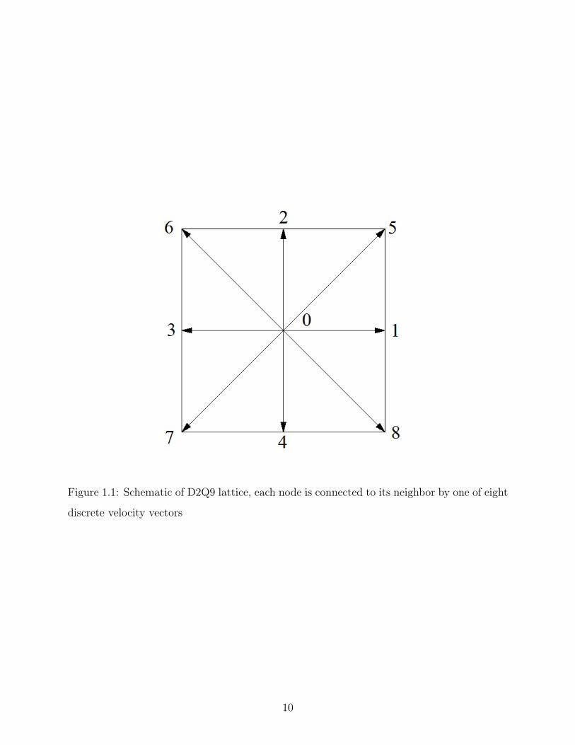
Figure 1.1: Schematic of D2Q9 lattice, each node is connected to its neighbor by one of eight

discrete velocity vectors

10

to relax toward a quasiequilibrium. This equilibrium is determined by the macroscopic

physical behavior of interest. In the case of incompressible flow, the quasiequilibrium particle

distribution, f eqi = f eqi (x, t), is often given by:

f eqi = wiρ

[1 +

ξi · uc2s

+(ξi · u)2

4c2s

− u2

2c2s

], (1.7)

where ρ and u are dependent on x and t, and wi is the weight in the ith:

wi =

49, i = 0

19, i = 1, 2, 3, 4

136, i = 5, 6, 7, 8

. (1.8)

Due to its simplicity and computational efficiency, the most common collision operator

is the Bhatnagar–Gross–Krook (BGK) operator. BGK consists of a single relaxation time

and is a linear relaxation of particle distributions toward equilibrium. The BGK collison

operator for the ith discrete velocity is expressed as:

Ωi(x, t) = −ω(fi(x, t)− f eqi (x, t)), (1.9)

where ω is the collision frequency [33]. The collision frequency can be related to macro-

scopic constitutive properties through Chapman-Enskog multiscale analysis [34]. For in-

compressible Newtonian flow, the collision frequency is related to the kinematic viscosity

by ν = c2s(

1ω− 1

2); and from this relationship it is clear that ω ∈ [0.0, 2.0], otherwise the

viscosity would be negative. The method for simulating non-Newtonian flow in the current

work involves approximating a solution to the local value of apparent viscosity, µapp(x, t),

using (1.1) where τ and γ are dependent on x and t, and then setting the value of the local

collision frequency as follows:

ω(x, t) =1

µapp(x,t)

c2sρ(x,t)+ 1

2

(1.10)

Despite the utility of the BGK collision operator, it does have a few drawbacks. For

example, in low viscosity fluids the BGK operator results in an overrelaxation of particle

distributions toward quasiequilibrium. It is well known that when large nonequilibrium

distributions exist in the LBM approximation that overrelaxation can result in nonphysical

11

oscillations that are slow to decay [26, 35]. To illustrate this, consider a flow in which there

is a sharp spatial gradient in either ρ or u at x. As f eqi depends on both ρ and u (1.7),

it may be the case that |f eqi (x, t) − f eqi (x + ξi∆t, t + ∆t)| >> 0, i.e. there may be a large

difference in the quasiequilibrium for the ith discrete velocity at (x, t) and (x+ξi∆t, t+ ∆t).

In this case, if fi is “near” to quasiequilibrium at x it will be “far” from quasiequilibrium

after the streaming step when it moves to the node at x + ξi∆t. Overrelaxation will occur

if ν → 0 because consquently ω → 2 and (1.9) results in fi(x + ξi∆t, t+ ∆t) still being “far”

from f eqi (x + ξi∆t, t+ ∆t) but on the “other side”. Overrelaxation in subsequent time steps

(along the streaming trajectory of fi) could result in nonphysical oscillations such as those

depicted in Figure 1.2. Considering the effect oscillations of particle distributions will have

on macroscopic variables and, consequently, local quasiequilibriums, positive feedback loops

can occur causing the system to diverge or “pollute” the system enough to make the results

highly nonphysical and altogether useless [29].

The challenge associated with high viscosity fluids is that particular distributions may

never relax as “far” toward quasiequilibrium as is physical because ω → 0 as ν →∞, resulting

in extreme underrelaxation to the point of being negligible.

Concerns with sharp gradients, overrelaxation, and underrelaxation are particularly rele-

vant in non-Newtonian flow because of the nonlinear constitutive relationship between shear

stress and strain-rate. The nonlinear constitutive relationship can lead to sharp gradients in

ρ or u, and depending on the form of the function µapp(γ), the apparent viscosity, µ(γ(x)),

may result in overrelaxation in certain parts of the domain and extreme underrelaxation in

others.

Due to the instabilities associated with the collision frequency being too high (e.g. ap-

proaching 2) or too low (e.g. approaching 0), a natural, albiet nonphysical, approach to

using the BGK collision operator for non-Newtonian flow is to simply put bounds on the

values in which the collision frequency may attain (such as in [18, 19, 22]). This simple

methodology for increasing stability will henceforth be referred to bounded-relaxation time

BGK, or BGK-BRT.

12

Figure 1.2: Example of oscillations that can occur as a result of overrelaxation; the collision

frequency, ω = 1.95 and µapp ≈ 0.0043

13

1.3.2.2 Multiple-relaxation Time (MRT) An alternative to the BGK collision oper-

ator is the multiple-relaxation-time (MRT) collision operator. In the LB-MRT scheme, one

constructs a space based on the particle velocity, ξ, moments of f =f0 f1 ... f8

, herein

referred to as the “moment space”. The collision is then performed in the moment space.

There are a few reasons why it is advantageous to perform the collision in the moment space

as opposed to the particle distribution space:

14

1. Physical processes in fluids can be approximately described by coupling or interacting

among modes, and the modes are directly related to the moments [17].

2. For the D2Q9 lattice, there are nine distribution functions, f0, f1, ..., f8, but only six

variables that affect the intended hydrodynamics on a macroscopic scale, namely: ρ, u,

and Π, where Π is the momentum flux tensor [35]. Of the nine relaxation rates available,

the three that correspond to the extra variables–often referred to as “ghost variables”,

and their associated modes as “ghost modes”–can be tuned in order to dampen out

their associated ghost modes, ensuring these modes do not dominate or cause numerical

instabilities at the lattice scale.

The MRT collision operator is given by:

Ω = −M−1SM(f − f eq), (1.11)

where M is a transformation matrix that maps the particle distribution vector, f , and

quasiequilibrium distribution vector, f eq, from the particle distribution space into moment

space. The result of mapping the vectors f and f eq into moment space will be denoted by m

and meq, respectively. The relationships between m, M and f can be written as follows:

m =

ρ

e

ε

jx

qx

jy

qy

pxx

pxy

=

1 1 1 1 1 1 1 1 1

−4 −1 −1 −1 −1 2 2 2 2

4 −2 −2 −2 −2 1 1 1 1

0 1 0 −1 0 1 −1 −1 1

0 −2 0 2 0 1 −1 −1 1

0 0 1 0 −1 1 1 −1 −1

0 0 −2 0 2 1 1 −1 −1

0 1 −1 1 −1 0 0 0 0

0 0 0 0 0 1 −1 1 −1

f0

f1

f2

f3

f4

f5

f6

f7

f8

= Mf . (1.12)

where ε is related to the square of the energy e; qx and qy correspond to the energy fluxes in the

x and y directions; and pxx and pxy correspond to the diagonal and off-diagonal component

of the viscous stress tensor [17]. The relaxation matrix, S, is a diagonal matrix where each

15

of the elements on the diagonal, si ∈ [0, 2], i = 0, 1, ..., 8, correspond to the relaxation rate

of its associated hydrodynamic mode. In the case when s0 = s1 = ... = s8 = ω (ω is the

collision frequency in the BGK sense), the MRT collision operator is equivalent to the BGK

collision operator. The relaxation parameters s0, s3, and s5 are all set to zero as mass and

momentum should be conserved. The relaxation parameters s1 and s7 = s8 are related to

the bulk and shear viscosities, respectively. The relationship for the shear viscosity is given

by:

ν = c2s∆t(

1

s7

− 1

2), (1.13)

which is equivalent with the relationship to the collision frequency, ω, in the BGK sense

(when ∆t = 1). The remaining relaxation parameters, s2, s4, and s6, are tuned in order to

dampen out and separate the ghost modes from the modes affecting hydrodynamic transport.

It is common practice, and [17] recommends, that these three relaxation parameters be set

to slightly larger than one.

The MRT collision operator has a greater numerical stability than its BGK counter-

part [17, 35, 36], and because of the challenges associated with simulating non-Newtonian

flow, the MRT collision operator has become popular for simulating non-Newtonian fluids [5–

9, 37]. The main drawback of the MRT collision operator is its computational expense. Why

MRT is more computationally expensive is clear when one considers that (1.11) requires

multiple matrix multiplications and (1.9) requires none. It has been reported that MRT is

approximately 15% slower than BGK [36], but this was in the context of Newtonian flow.

As will be shown later, for certain LBM implementations and non-Newtonian fluid flows the

increase in computational expense can be much greater.

1.3.3 Stability Enhancement through Artificial Dissipation: Entropic Filtering

To reduce nonequilibrium fluctuations in LBM, one can introduce artificial dissipation. The

idea of artificial dissipation is to increase numerical stability, while sacrificing some physical

accuracy. A model that has more physical justification but produces unstable and nonsensical

results is much less useful than a model with some minor artificial features yet produces more

stable results. A practical goal then would be to use only the necessary amount of artificial

16

dissipation in order to ensure a stable solution. From this goal two questions naturally arise:

“under what criteria does one decide that artificial dissipation is necessary?” and “how much

artificial dissipation does one introduce when it is necessary?”.

To answer the first question, consider the discussion in Section 1.3.2.1 on problems with

overrelaxation and nonphysical oscillations. Nonphysical oscillations due to overrelaxation

would be damped out more quickly if particle distributions “far” from quasiequilibrium were

brought closer to quasiequilibrium. A particle distribution vector, f , “far” from equilibrium

would be a good candidate for artificial dissipation. There are many ways one can measure

the distance between f and f eq; for example, a reasonable choice would be ||f − f eq||p for

some p norm. A metric that has been developed and used successfully for determining

when artificial dissipation should be introduced at a lattice site is the so called relative

nonequilibrium entropy [25–29]. The relative nonequilibrium entropy, ∆S, is given by:

∆S =∑i

fi ln(fif eqi

). (1.14)

A more computationally efficient approximation of ∆S can be achieved by instead using the

second order Taylor expansion of (1.14):

∆S ≈∑i

(fi − f eqi )2

2f eqi. (1.15)

Note that limiting nonequilibrium entropy in LBM is analogous to what flux limiters do in

finite difference, finite volume, and finite element methods [27].

A criteria for introducing artificial dissipation that has been used successfully [25–27, 29]

is to define a threshold, θ, such that dissipation is added when:

∆S(x, t) > θ. (1.16)

A potential drawback of defining a threshold a priori is that in order to ensure the model still

retains some physical integrity, only a small number of sites can have artificial dissipation

added. If the threshold is too low, too many sites may have dissipation added. If the threshold

17

is too high, a stable solution may not be achieved. The threshold can be determined on a

case-by-case basis through trial-and-error or by a preliminary analysis. In the current work,

the criteria that is used for determining whether dissipation should be added is a combination

of (1.16) and the following:

∆S(x, t) > ∆S + nσ · σ∆S, (1.17)

where ∆S and σ∆S are the mean and standard deviation of ∆S, respectively–both are

calculated using values over the domain for the current timestep–and nσ is the number of

standard deviations greater than ∆S that ∆S must be before dissipation is added. The

number of standard deviations, nσ, is chosen a priori. The criteria described in (1.17) has

the advantage that one does not need to determine a priori what constitutes “far” from

quasiequilibrium, but instead can think in terms of what would be the maximum percentage

of sites one would want artificial dissipation to be added to. A disadvantage of (1.17) is that

if ∆S and nσ are both small then it is possible for dissipation to be added when ∆S(x, t) is

low and artifical dissipation is unnecessary. By required that both (1.16) and (1.17) be met

before artifical dissipation is added, there is the potential for (1.16) and (1.17) to compensate

for the each other’s disadvantage.

Just as there are many ways to measure a lattice site’s distance from quasiequilibrium,

or from that measure define criteria for artificial dissipation, there are also many different

ways of deciding how much dissipation to add. One method of adding dissipation is the

so-called Ehrenfests’ regularization [25], and involves setting a lattice site that is chosen

for artificial dissipation to its quasiequilibrium state. Although this achieves the desired

result, namely damping out large nonequilibrium fluctuations, it does so in a way that

is not smooth or gradual, but sharp. An alternative, the median filter, has been used

successfully in conjunction with both the BGK and MRT collision schemes for simulating one-

dimensional shock tubes and lid-driven cavity flow [27–29]. Median filtering is an effective

noise reduction technique, often used in image processing, for “speckle noise” or “salt and

pepper noise” [27]. In other words, median filters are good at reducing high frequency noise

while having a minimal effect on lower frequency noise. In LBM this is a desirable way to

introduce dissipation because it has the potential to reduce high frequency nonequilibrium

18

fluctuations that might lead to numerical instability while retaining the lower frequency

dynamics. To use the median filter one performs the collision step and then checks over the

domain for lattice sites with ∆S that meet the criteria for artificial dissipation; sites that

meet the criteria are updated as follows:

f = f eq + δ(f − f eq), (1.18)

where δ =√

∆Smed/∆S is the scaling coefficient, and ∆Smed is the median value of ∆S for

the nearest neighbors of the lattice site.

1.3.4 Boundary Conditions

No slip, or zero velocity, which is commonly imposed at walls in a domain, is accomplished by

simulating the particle distributions as "bouncing back" at the walls in the opposite direction

from which they stream. For example, for a particle distribution streaming in the direction of

a south wall, f2 = f4, f5 = f7, and f6 = f8. For velocity or pressure boundary conditions, the

method proposed by [38] can be used. The particle distributions that are missing after the

streaming step are solved for by assuming a bounceback of the nonequilibrium distribution

in the direction normal to the boundary; e.g., for a south inlet or outlet, f2− f eq2 = f4− f eq4 .

19

1.3.5 Applied Forces

Incorporating external forces, such as gravity, pressure gradients, etc., is done by adding

a source of particle distributions in the direction of the force. The increase in particle

distributions leads to the desired macroscopic result–an increase in momentum. The LBE

with external forces is:

fi(x + ξi∆t, t+ ∆t) = fi(x, t) + Ωi(f) +wi∆t

c2s

F · ξi (1.19)

where F is the body force vector.

1.3.6 Strain-rate Tensor

In order to solve for the apparent viscosity, µapp, using the Picard-type algorithm outlined

in Section 1.2, one must calculate the strain-rate, γ. The strain-rate is given by the second

invariant of the strain-rate tensor, Dαβ, i.e.:

γ =

√√√√22∑

α,β=1

DαβDαβ. (1.20)

When using the BGK collision scheme, the strain-rate tensor is determined by:

Dαβ = − ω

2ρc2s

∑i

ξiαξiβ(fi − f eqi ), (1.21)

and for the MRT collision scheme, the strain-rate tensor is determined by:

Dαβ = − 1

2ρc2s∆t

∑i

ξiαξiβ∑j

(M−1SM)ij(fi − f eqi ). (1.22)

Computing the strain-rate tensor by either (1.21) or (1.22) is second order accurate in

space [4, 39].

Upon comparison of (1.21) and (1.22), it is clear that calculating the strain-rate tensor

for the MRT collision operator is more computationally expensive than it is for the BGK

collision operator. The increase in computational expense is exacerbated by the fact that

approximating the apparent viscosity, µapp, by the algorithm outlined in Section 1.2 requires

iteration and therefore multiple calculations of the strain-rate tensor.

20

1.3.7 Non-Newtonian Constitutive Equations

1.3.7.1 Bingham Plastic The Bingham plastic constitutive model is popular for yield

stress flow. A Bingham plastic does not flow, i.e. the strain-rate is zero, when the shear stress

is below the yield stress, and behaves in an almost Newtonian manner when the shear stress

is above the yield stress. The Bingham plastic relationship is described mathematically as:τ = τy + µpγ, |τ | ≥ τy

γ = 0, |τ | < τy

(1.23)

where τ is the shear stress, τy is the yield stress, and µp is the plastic viscosity [40].

Due to the discontinuous nature of (1.23), the Bingham plastic model is difficult to work

with numerically. Thus, a smooth approximation to (1.23) formulated by [41] is often used

as:

τ = τy(1− e−m|γ|) + µpγ, (1.24)

where m is the stress growth exponent. The larger the value of m, the closer the approxi-

mation is to the Bingham plastic model.

Alternatively, the constitutive relationship can be interpreted through the apparent vis-

cosity. Noting that µapp = τγand rearranging (1.24) results in the following expression for

the apparent viscosity:

µapp =τyγ

(1− e−m|γ|) + µp. (1.25)

1.3.7.2 Power-law The power-law constitutive relationship is useful for modeling fluids

that experience shear-thinning or shear-thickening. The power-law relationship is given by:

τ = kγn, (1.26)

where k is the flow consistency index and n is the flow behavior index. When n = 1,

(1.26) results in a Newtonian constitutive relationship with dynamic viscosity, µ = k. A

flow consistency index of n < 1 results in shear-thinning behavior, where as n > 1 results

in shear-thickening. As with the Bingham plastic relationship, (1.26) can be modified to

determine an apparent viscosity:

µapp = kγn−1. (1.27)

21

1.4 NUMERICAL STUDY

A numerical study was carried out in order to investigate the suitability of different LBM

collision schemes for simulating non-Newtonian flow in terms of accuracy, numerical stability

and computational efficiency. For all simulations presented in this section, the apparent

viscosity is approximated using its corresponding constitutive relationship and the Picard-

type algorithm outlined in Section 1.2 with the maximum number of iterations set at 15 and

the convergence criteria: ∣∣µk+1app − µkapp

∣∣µkapp

< 1.0× 10−6. (1.28)

All BGK-BRT collision schemes use ω ∈ [0.05, 1.995] as the bounds on the collision frequency.

All simulations with artificial dissipation use the median filter with θ = 1.0 × 10−6 and

nσ = 2.7 where θ is the threshold that ∆S(x, t must exceed before dissipation is added

(1.16) and nσ is the number of standard deviations greater than ∆S that ∆S(x, t) must be

before dissipation is added (1.17). All numerical values given in this section are in lattice

units unless otherwise stated.

1.4.1 Poiseuille Flow

Poiseuille flow is a useful benchmark because analytical solutions exist for both Bingham

plastic and power-law fluids. Poiseuille flow is driven by a constant pressure gradient, ∂p∂x,

through a two-dimensional channel. A schematic is shown in Figure 1.3. No-slip boundary

conditions are enforced at the top and bottom boundaries with a wall velocity of zero so that

u× n = 0 where n is the unit normal vector to the boundary. Periodic boundary conditions

are enforced at the left and right boundaries. The total height of the channel is denoted by

H. The center of the channel is y = 0 and y ∈ [−h, h] where h = H2.

Unless otherwise stated, all of the Poiseuille flow simulations were computed on a 32×64

lattice for 25000 timesteps. The lattice size was chosen to be sufficiently fine for accuracy

(although the length, L = 32, seems small, the effect is negligible as the east-west boundary

conditions are periodic) and the number of time steps were set high enough to ensure a

steady-state would be reached. In reference to computational time, each of the simulations

22

Figure 1.3: Schematic of Poiseuille flow; no-slip boundary conditions are enforced at the top

and bottom boundaries, and periodic boundary conditions are enforced at the left and right

boundaries. The size of the domain is L = 32 and H = 64.

23

in this section were run on a single core of an Intel I7-860 Quad-Core 2.80GHz processor.

For the MRT relaxation matrix the free parameters were set to s1 = s2 = s4 = s6 = 1.1,

which follows the recommendation of [17] for reasons of stability, and has been successfully

used to simulate non-Newtonian flow in the past [7, 37].

1.4.1.1 Bingham Plastic Fluids The Bingham plastic simulations were carried out

with a pressure gradient of ∂p∂x

= 1.0 × 10−5, and a plastic viscosity of µp = 0.2. The yield

stress was varied between four different values τy = [4.0, 8.0, 12.0, 16.0] × 10−5, and four

different LBM schemes were used: (1) BGK with m = 105, (2) BGK with m = 108, (3)

BGK with m = 108 and the median filter, and (4) MRT with m = 108. Recall that m is the

stress growth exponent for the Papanastasiou approximation. The relative L2 and relative

L∞ errors with respect to the analytical solution were computed for each simulation. The

analytical solution for Poiseuille flow of a Bingham plastic fluid is given by:

ux(y) =

1

2µp

(− ∂p∂x

)[h2 − y2

τ ]−τyµp

(h− yτ ) , 0 ≤ |y| ≤ yτ ,

12µp

(− ∂p∂x

)[h2 − y2]− τy

µp(h− |y|) , yτ < |y| ≤ h,

(1.29)

where yτ = −τy/ ∂p∂x is the vertical location at which the fluid yields.

The relative L2 error, relative L∞ error, and computation time for each simulation are

presented in Table 1.1. The Reynold’s number was computed by Re = ρUHµp

, where U is the

maximum velocity given by the analytical solution. The Bingham number was computed by

Bn = τyH

µpU.

As has been reported previously, for the BGK collision operator, using a stress growth

exponent of m = 105 is more accurate with respect to the analytical solution than using

a stress growth exponent of m = 108 [8]. A larger stress growth exponent results in a

more accurate Papastasiou approximation of the true Bingham plastic constitutive model,

however, it leads to more nonphysical oscillations that degrade the numerical solution for

the BGK collision operator. Upon inspection of Table 1.1, it does not appear that entropic

24

Table 1.1: Bingham plastic Poiseuille flow

Collision

Operator

Median

Filterm

τy

(×10−5)Re Bn L2 L∞

Time

(sec)

BGK No 105 4.0 6.05 0.68 0.0062 0.0153 1857

8.0 4.42 1.85 0.0204 0.0411 2329

12.0 3.04 4.04 0.0503 0.0891 3345

16.0 1.92 8.52 0.1161 0.1879 2029

BGK No 108 4.0 6.05 0.68 0.0109 0.0282 2831

8.0 4.42 1.85 0.0330 0.0670 3509

12.0 3.04 4.04 0.0788 0.1570 4838

16.0 1.92 8.52 0.1991 0.3539 3790

BGK Yes 108 4.0 6.05 0.68 0.0100 0.0273 2903

8.0 4.42 1.85 0.0361 0.0823 3567

12.0 3.04 4.04 0.2439 0.3832 4800

16.0 1.92 8.52 0.7533 1.0718 3507

MRT No 108 4.0 6.05 0.68 0.0013 0.0013 5914

8.0 4.42 1.85 0.0018 0.0018 7908

12.0 3.04 4.04 0.0026 0.0026 7160

16.0 1.92 8.52 0.0041 0.0041 5559

25

median filtering helps mitigate errors that occur as a result of using m = 108 for Bingham

plastic Poiseuille flow. In fact, the median filter resulted in a less accurate solution in all

cases other than the case with the lowest yield stress considered (i.e., the smoothest flow

field), and rendered the solution altogether useless for the higher yield stress fluids (relative

errors of approximately 25-75%).

In general, the BGK collision operator using a stress growth exponent ofm = 105 had the

lowest computational time. This can be attributed to the fact that a smoother approximation

of the Bingham plastic constitutive model would lead to a solution for µapp converging with

less iterations. The BGK collision operator using a stress growth exponent of m = 105

experienced relatively low error for lower yield stress fluids, however, for τy = 12× 10−5 and

16× 10−5 the relative L∞ errors were 8.9% and 19%, respectively, which is larger than what

would be considered acceptable for most engineering applications.

The LBM approximations of the velocity profile across the channel (more specifically,

ux(xj, 25000) where xj =

16 yj

Tfor j = 1, 2, ..., 64, i.e. xj is taken at 16 nodes in

from the left in the x-direction and for the full height of the channel in the y-direction) for

the BGK collision operator using m = 105 and m = 108 are plotted with the analytical

solution (1.23) in Figure 1.4 and Figure 1.5, respectively. Due to the smoothness of the

LBM approximation in Figure 1.4, one can conclude that the error for the BGK model with

m = 105 is not due to nonphysical oscillations, but instead the inaccuracy of the Papastasiou

approximation with a lower stress growth exponent. In contrast, the LBM approximation in

Figure 1.5 is not smooth, which suggests that the error for the BGK model with m = 108 is

due to nonphysical oscillations.

In order to better understand why median filtering did not eliminate the nonphysical

oscillations in high yield stress fluids, but instead exacerbates the problem, it is necessary to

investigate what is happening at the particle distribution scale. Figure 1.6 compares particle

distributions to quasiequilibrium. More specifically, Figure 1.6 compares fi(xj, 25000) to

f eqi (xj, 25000) where xj =

16 yj

Tfor j = 1, 2, ..., 64, and i = 5, 8. It can be seen that

in the BGK, m = 108 solution, that nonphysical oscillations pollute the quasiequilibrium

profile as well. These nonphysical oscillations likely originate at the lattice scale due to

the sharp gradient in the macroscopic velocity, u, near the walls, and the sharp gradient

26

Figure 1.4: LBM approximation using BGK andm = 105 compared to the analytical solution

for τy = 16× 10−5.

27

Figure 1.5: LBM approximation using BGK andm = 108 compared to the analytical solution

for τy = 16× 10−5.

28

in u is a result of a sharp gradient in µapp, namely the sharp gradient of the constitutive

relationship. Because the nonphysical oscillations make their way into the quasiequilibrium

values, entropic median filtering does not help dampen the oscillations but instead contracts

the particle distributions closer to the quasiequilibrium oscillations, which explains why the

median filtered results were less accurate for Bingham plastic Poiseuille flow. In order to

ensure that this phenomena was a side effect of all entropic filtering, and not just entropic

median filtering with θ = 1.0 × 10−6 and ns = 2.7, optimization was used to find the value

of θ that minimized error for both median filtering and Ehrenfests’ regularization. The

optimization problem was defined as follows:

minθ

f(θ)

such that θ ∈ [10−10, 2.0]

where f(θ) ≡ the relative L2 error between the LBM approximation using m = 108 and

entropic filtering with a ∆S threshold of θ (used in the criteria defined in (1.16)). The

bounds on θ, namely θ ∈ [10−10, 2] represent θ such that 100% of lattice sites are filtered for

every time step (θ = 10−10) and θ such that no lattice sites are filtered for any time step

(θ = 2.0). The optimization problem was solved for the cases of using median filtering and

Ehrenfests’ regularization using both Brent’s method and the Golden Section search. For

all four cases, the optimal solution was θ = 2.0 and the cost function, f(2.0), was equal to

the relative L2 error for the BGK collision operator, m = 108 and no entropic filtering. The

results of the optimization suggest that entropic filtering, at best does not affect the accuracy

of LBM, and often adversly affects the accuracy of LBM in approximating Bingham plastic

Poiseuille flow, regardless of whether median filtering or Ehrenfests’ regularization is used,

and regardless of what the ∆S threshold, θ, is set to. Thus, entropic filtering is not effective

for increasing the accuracy of Bingham plastic Poiseuille flow.

On average, the LBM model using the MRT collision operator took 2.9 times more

computation time than the BGK collision operator with m = 105. However, the increased

computational time can be justified for the MRT collision operator because MRT solution did

not suffer from the same level of nonphysical oscillations as the BGK collision operator when

using the more accurate approximation of the Bingham plastic model, i.e. when m = 108.

29

Figure 1.6: Particle distributions in the 5 direction (left) and 8 direction (right) compared

to their respective quasiequilibriums. The top two plots are for the BGK with m = 105, the

bottom two are for the BGK with m = 108.

30

Figure 1.7: Particle distributions in the 5 direction (left) and 8 direction (right) compared

to their respective quasiequilibriums for the MRT with m = 108.

The MRT collision operator was therefore the most accurate solution for all cases. Figure 1.7

compares particle distribution, fi, profiles to their respective quasiequilbirium profiles, f eqi for

the MRT model; in contrast to the BGK with m = 108, there are no nonphysical oscillations

in the quasiequilibrium distributions.

Another important question to ask is, if the strength of the MRT collision operator

is damping out the ghost modes, then are the nonphysical oscillations for the BGK with

m = 108 (with and without median filtering) a result of the ghost modes?. Figure 1.8 shows

a measure of the nonequilibrium ε moment, εneq, with respect to time for each of the collision

schemes, which was calculated as:

||ε− εeq||2||εeq||2

(1.30)

where || . . . ||2 is the Euclidean norm, εj = 4f0(xj)− 2f1(xj)− 2f2(xj)− 2f3(xj)− 2f4(xj) +

f5(xj)+f6(xj)+f7(xj)+f8(xj) is related to the square of the energy, and xj =

16 yj

Tfor

j = 1, 2, ..., 64, i.e. xj is taken at 16 nodes in from the left in the x-direction and for the full

height of the channel in the y-direction. The values measured for the BGK with m = 108,

31

with and without median filtering, were significantly higher than for either the MRT or BGK

with m = 105 collision schemes, which suggests that the nonphysical oscillations the BGK

with m = 108 suffered from was in part due to the ε moment.

Figure 1.9 shows a measure of the nonequilibrium qx moment, qxneq, or energy flux in

the x-direction, with respect to time for each of the collision schemes, which was calculated

as:||qx − qx

eq||2||qx

eq||2(1.31)

where qxj = −2f1(xj) + 2f3(xj) + f5(xj)− f6(xj)− f7(xj) + f8(xj) and xj were taken across

the height of the channel in the same manner as with the ε moment. The values measured

for the BGK with m = 108 and median filtered were consistently greater than any other

collision scheme. The relative L2 norm of the qxneq for the BGK collision operator with

m = 108 and median filtering solution spent most of the simulation between approximately

50% and 100%, this suggests that the qx moment was likely the cause of the nonphysical

oscillations and error in its solution. As expected (if the dominant source of error in the

LBM approximation for Bingham plastic Poiseuille flow is indeed due to the qx moment),

the qneqx relative L2 norm for the BGK with m = 108 was slightly greater than the BGK

with m = 105, and the qneqx relative L2 was negligible for the MRT collision scheme. These

results are consistent with solution error.

It is likely that the nonequilibrium ε and qx moments cause nonphysical oscillations in

particle distributions, fi, with a cumulative effect in time, i.e. osciallations build in amplitude

with time. Figure 1.10 and Figure 1.11 show the cumulative measures of the nonequilibrium

moments in time, which was calculated as:

∫ T

0

||ε(t)− εeq(t)||2||εeq(t)||2

dt, (1.32)

and, ∫ T

0

||qx(t)− qxeq(t)||2

||qxeq(t)||2

dt, (1.33)

where T is the current time. Figure 1.9 and Figure 1.11 shows that both the peak and cumu-

lative values of the relative L2 norm of qxneq are much larger than the peak and cumulative

values of the relative L2 norm of εneq, which suggests that the ghost mode associated with

32

Figure 1.8: Evolution of relative L2 norm, εneq with time. The norm of the εneq across the

height of the channel is an indicator of an increase in oscillations at the lattice level due to

the ε moment.

33

Figure 1.9: Evolution of relative L2 norm, qxneq with time. The norm of the qneq

x across the

height of the channel is an indicator of an increase in oscillations at the lattice level due to

the qx moment.

34

the qx moment dominates and is the primary source of oscillations. It can be inferred that

the qx moment was significant source of oscillations in this case because the Poiseuille flow

was in the x-direction. If an LBM collision scheme is to be developed for simulating high

yield stress, Poiseuille-type flow that is more accurate than the BGK with m = 105 and

more computationally efficient than the MRT, it should focus on a means of dampening the

nonequilibrium energy flux moments, namely qx and qy.

1.4.1.2 Power-law Fluids The simulations of the Poiseuille flow with the power-law

constitutive relationship were carried out with a pressure gradient of ∂p∂x

= 1.0 × 10−5,

and a flow consistency index of k = 0.2. The flow behavior index, n, was varied between

the four different values: [0.5, 0.75, 1.25, 1.50], and four different LBM schemes were used:

(1) BGK, (2) BGK with median filtering, (3) MRT, and (4) BGK-BRT, with ω bounded

within [0.05, 1.995]. The relative L2 and relative L∞ errors with respect to the analytical

solution were computed for each simulation. The analytical solution for the velocity profile

of Poiseuille flow with the power-law constitutive relationship is given by:

ux(y) =n

n+ 1

(−1

k

∂p

∂x

)1/n [h

n+1n − |y|

n+1n

]. (1.34)

The relative L2 error, relative L∞ error, and computation time for each simulation are

presented in Table 1.2. The Reynold’s number was computed by Re = ρU2−nHn

k.

Although for n = 0.5, 0.75, 1.25 the MRT collision operator was more accurate and

required more computation time than the BGK collision operator, for n = 1.5 the BGK

operator with median filtering required the least computation time and was the most accurate

with respect to the analytical solution. In fact, besides for the case of n = 0.5, i.e. relatively

extreme shear-thinning, the BGK with median filtering was both computationally efficient

and accurate. The BGK-BRT had a moderate improvement of accuracy and efficiency–with

respect to the regular BGK collision scheme–for flow where the constitutive relationship was

only somewhat nonlinear, i.e. for n = 0.75, 1.25. Note that none of the collision schemes

were sufficiently accurate (error greater than 15%) for the case of n = 0.5, and to improve

this accuracy it would be necessary to use a different simulation Mach number, a finer grid,

and/or a smaller pressure gradient.

35

Figure 1.10: Cumulative relative L2 norm, εneq with time. Oscillations can have a positive

effect on each other, building up. The cumulative relative L2, εneq is a measure of how much

oscillations due to the ε moment may have been building in time.

36

Figure 1.11: Cumulative relative L2 norm, qneqx with time. Oscillations can have a positive

effect on each other, building up. The cumulative relative L2, qneqx is a measure of how much

oscillations due to the qx moment may have been building in time.

37

Table 1.2: Power-law Poiseuille flow

Collision

Operator

Median

Filtern Re L2 L∞

Time

(sec)

BGK No 0.50 0.0007 28.06 30.37 5232

0.75 0.9125 0.0328 0.0569 2399

1.25 423.2 0.0051 0.0055 2311

1.50 2213 1.0 1.0 3622

BGK Yes 0.50 0.0007 26.72 28.78 5347

0.75 0.9125 0.0328 0.0569 2385

1.25 423.2 0.0051 0.0055 2275

1.50 2213 0.0570 0.0600 2357

MRT No 0.50 0.0007 0.1758 0.1401 4906

0.75 0.9125 0.0058 0.0045 4880

1.25 423.2 0.0051 0.0055 4863

1.50 2213 1.0 1.0 15992

BGK-BRT No 0.50 0.0007 11.73 12.56 4450

0.75 0.9125 0.0320 0.0475 1805

1.25 423.2 0.0051 0.0055 1905

1.50 2213 1.0 1.0 8194

38

1.4.2 Lid-driven Cavity Flow

The lid-driven benchmark was chosen for this numerical study because there are many results

available in literature in which to compare with and because the vorticity of the flow coupled

with the nonlinear constitutive equations should result in a challenge in terms of stability.

Lid-driven cavity flow is generally characterized by a square cavity where a fluid velocity

is prescribed tangential to the upper boundary and the remaining boundaries have a no-

slip boundary condition. The example of lid-driven cavity flow utilized herein is presented

schematically in Figure 1.12.

The lid-driven cavity simulations presented in the section were all simulated on a rel-

atively coarse, 100 × 100 lattice (other studies simulating lid-driven cavity flow of a non-

Newtonian fluid tend to use lattice sizes on the order of 256 × 256 and 512 × 512 [8, 42],

this study follows that of [27]). A coarse lattice was chosen in order to highlight concerns

with stability and accuracy. The simulations were run for either 50000 timesteps or until

convergence was met. Convergence was defined by,

100∑m=1

∑i,j

|uki,j − uk−mi,j ||uk−mi,j |

< 1.0× 10−7, (1.35)

where i is the node index in the x-direction, j is the node index in the y-direction, and k is

the current timestep. The lid velocity was prescribed as uo = 0.1. For the MRT relaxation

matrix, the free parameters were set to s1 = 1.1, s2 = 1.0, and s4 = s6 = 1.2 as these

values have been successfully applied to simulating lid-driven cavity flow of non-Newtonian

fluids in the past [8, 42]. All coordinate values presented in this section (used to describe

the location of the center of vortices) are given normalized with respect to the length of the

cavity side, i.e. as (x/L, y/L). Note that all results presented as “-” indicate that the tests

were numerically unstable to the extent that the degrees of freedom all over the domain were

nonsensical.

39

Figure 1.12: Schematic of lid-driven cavity flow; a velocity is prescribed tangential to the

top boundary and no-slip is enforced at the remaining boundaries. L = 100

40

1.4.2.1 Bingham Plastic Fluids For the Bingham plastic numerical tests the Reynold’s

number was varied:[100, 1000, 5000, 10000], and the Bingham number was varied: [1, 10, 100]

(Bn and Re were calculated the same as in Section 1.4.1.1). The collision schemes that were

tested were: (1) BGK with m = 105, (2) BGK with m = 108, (3) BGK-BRT with m = 108,

(4) BGK with m = 108 and median filtering, (5) MRT with m = 108 and (6) MRT with

m = 108 and median filtering. Tables 1.3–1.5 compare the center location of the main vortex

to literature values taken from [43]. The main vortex location is determined by calculating

the stream function using Simpson’s rule and finding where it attains a maximum.

Just as before with the Bingham plastic Poiseuille flow, if a modeler is using the BGK

collision operator and entropic filtering is not available, a stress growth exponent of m = 105

yields faster, more accurate results than using a larger stress growth exponent. A smaller

stress growth exponent is also more effective at producing accurate results in the BGK

collision scheme than placing bounds on the relaxation time (BGK-BRT). However, although

the BGK with m = 105 was the fastest model in all cases, it was also like the other two BGK

models without median filtering in that it was unstable for Re ≥ 5000.

For flow with Re ≥ 5000, the BGK with m = 108 and median filtering produced nu-

merically stable results. However, in general, the BGK with m = 108 and median filtering

was consistently different from literature values. The apparent inaccuracy with regards to

BGK with m = 108 and median filtering is probably due to how the numerical stability is

enhanced–namely through artificial, nonphysical dissipation. In contrast to the nonphysical

nature in which median filtering enhances stability, the stability enhancement used by MRT

does not directly affect the macroscopic hydrodynamics of interest, so it again provides a

stable, and in most of the cases examined herein, the most accurate solution. The apparent

superiority in terms of stability and accuracy of the MRT collision operator still comes at

a price though. The MRT collision operator was, in general, 5-10 times slower than any of

the BGK collision schemes. The extreme increase in computational expense is probably not

due to the collision process itself, i.e. (1.11), but instead calculating the strain-rate (1.22)

for each iteration of the solution for µapp.

41

Table 1.3: Bingham plastic, lid-driven cavity flow; Bn = 1.

Bn ReCollisionOperator

MedianFilter

m

VortexCenter(literature)

VortexCenter(LBM)

Time(sec)

1 100 BGK No 105 (0.63, 0.79) (0.63, 0.79) 17685BGK No 108 (0.63, 0.79) 19398BGK-BRT No 108 (0.63, 0.79) 22656BGK Yes 108 (0.63, 0.79) 21535MRT No 108 (0.63, 0.79) 79040MRT Yes 108 (0.63, 0.79) 85295


1 5000 BGK No 105 (0.52, 0.53) - -BGK No 108 - -BGK-BRT No 108 - -BGK Yes 108 (0.54, 0.53) 17248MRT No 108 (0.51, 0.55) 50572MRT Yes 108 (0.52, 0.53) 54225

1 10000 BGK No 105 N/A - -BGK No 108 - -BGK-BRT No 108 - -BGK Yes 108 (0.56, 0.60) 18186MRT No 108 (0.48, 0.48) 43246MRT Yes 108 (0.46, 0.54) 50864

42



MedianFilter

m


VortexCenter(LBM)

Time(sec)




10 10000 BGK No 105 N/A - -BGK No 108 - -BGK-BRT No 108 - -BGK Yes 108 (0.49, 0.54) 19351MRT No 108 (0.53, 0.54) 69249MRT Yes 108 (0.53, 0.53) 69054

43



MedianFilter

m


VortexCenter(LBM)

Time(sec)





44

In summary for the lid-driven cavity flow of a Bingham plastic fluid,

• for low Reynold’s number flow the BGK collision operator with m = 105 provides an

accurate solution with a short computation time,

• for high Reynold’s number flow the BGK collision operator requires entropic filtering to

remain stable,

• and the MRT collision operator with m = 108 produces solutions with high accuracy and

stability for all of the cases examined herein, but at an increased (approximately 5-10

times more) computational cost.

1.4.2.2 Power-law Fluids For the power-law numerical tests the Reynold’s number was

varied: [100, 1000, 5000, 10000], and the flow behavior index, n, was varied: [0.5, 1.5] (Re was

calculated the same as in Section 1.4.1.2). The collision schemes that were tested were: (1)

BGK, (2) BGK-BRT, (3) BGK with median filtering, (4) MRT with m = 108 and (5) MRT

with m = 108 and median filtering. Table 1.6 and Table 1.7 compare the center location of

the main vortex to literature values taken from [42].

For the shear-thinning results, n = 0.5, at the lowest Reynold’s number considered,

Re = 100, all of the collision schemes produced results that agreed well with the literature

value. However, the solutions became unstable at higher Reynold’s numbers and entropic

filtering was necessary to produce a stable soltuion when Re ≥ 1000 for the BGK collision

operator, and when Re ≥ 5000 for the MRT collision operator. Although there still appears

to be somewhat of a tradeoff between computational efficiency and accuracy in regards to

the BGK with median filtering and MRT with median filtering, it does not seem to be nearly

as drastic as when simulating Bingham plastic lid-driven flow; e.g. neither collision scheme

consistently agrees with the literature values; and the MRT with median filtering is only

2-3 times slower than the BGK with median filtering. A good example of this tradeoff is

the shear-thinning results for Re = 5000: the location of the main vortex for the BGK with

median filtering differed from literature by more than 10% in both the x and y directions

but the MRT with median filtering has approximately twice the computational cost.

45

Table 1.6: Power-law, lid-driven cavity flow; n = 0.5.

n ReCollisionOperator

MedianFilter


VortexCenter(LBM)

Time(sec)

0.5 100 BGK No (0.72, 0.78) (0.71, 0.77) 21429BGK-BRT No (0.71, 0.77) 14547BGK Yes (0.72, 0.78) 33221MRT No (0.71, 0.77) 77287MRT Yes (0.71, 0.77) 110403

0.5 1000 BGK No (0.58, 0.55) - -BGK-BRT No - -BGK Yes (0.53, 0.59) 24935MRT No (0.53, 0.54) 72102MRT Yes (0.53, 0.54) 78300

0.5 5000 BGK No (0.53, 0.52) - -BGK-BRT No - -BGK Yes (0.63, 0.68) 23517MRT No - -MRT Yes (0.51, 0.58) 54225

0.5 10000 BGK No (0.53, 0.52) - -BGK-BRT No - -BGK Yes (0.50, 0.55) 22603MRT No - -MRT Yes (0.50, 0.54) 63892

46

Table 1.7: Power-law, lid-driven cavity flow; n = 1.5.

n ReCollisionOperator

MedianFilter


VortexCenter(LBM)

Time(sec)





47

For the shear-thickening results, n = 1.5, there were no issues of stability. What is

interesting is that all of the collision schemes produce similar results for each of the cases,

with the difference in the location of the main vortex being no greater than 1% in either the x

or y direction for any two collision schemes (with the exception of the high Reynold’s number

case, Re = 10000). The BGK-BRT consistently needed the least amount of computation

time. The reason the BGK-BRT may be the most efficient is that because the collision

frequency, ω, is bounded, and consequently µapp is bounded, meaning the solution to the

constitutive equation may be converging to a bound with less iterations than the other

collision schemes.

1.5 CONCLUSIONS

A numerical investigation into the accuracy, stability, and efficiency of LBM collision models

when applied to non-Newtonian flow was presented. The numerical investigation included

testing the BGK and MRT collision operators, with and without entropic filtering, as applied

to Bingham plastics and power-law fluids. Two different benchmark problems were chosen

for the study: Poiseuille flow, and lid-driven square cavity flow. The results showed that:

• For high yield stress fluids in Poiseuille-type flow, only the MRT collision operator did

not suffer from nonphysical oscillations.

– The oscillations appeared to be due to high nonequilibrium values for the moment

related to the square of the energy, ε, and the energy flux moment in the direction

of flow, qx.

– If a collision scheme is to be developed for high yield stress, Poiseuille-type flow that

is more accurate than the BGK with m = 105 and more computationally efficient

than the MRT, then it should focus on dampening the nonequilibrium energy flux

moment.

• Median filtering can be an effective technique for enhancing stability, especially for high

Reynold’s number flow; however, if the filter is not carefully tuned by properly adjusted

48

the threshold, δ, or number of standard deviations, ns, then the physical intregrity, and

consquently accuracy, of the model can be adversely impacted.

• In general, the MRT collision operator is much more computationally expensive than its

BGK counterpart and is some times even orders of magnitude slower.

• To summarize Bingham plastic, lid-driven cavity flow,

– for low Reynold’s number flow the BGK collision operator with m = 105 provides

an accurate solution with a short computation time,

– for high Reynold’s number flow the BGK collision operator requires entropic filtering

to remain stable.

• To summarize power-law, lid-driven cavity flow,

– for shear-thinning fluids at high Reynold’s numbers (Re ≥ 5000) median filtering is

necessary to produce a stable solution,

– for shear-thickening, lid-driven cavity flow, there is much less concern for numerical

instability.

49

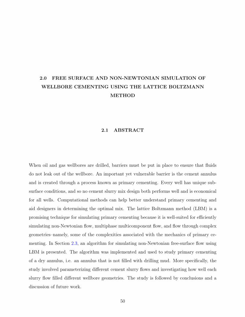
2.0 FREE SURFACE AND NON-NEWTONIAN SIMULATION OF

WELLBORE CEMENTING USING THE LATTICE BOLTZMANN

METHOD

2.1 ABSTRACT

When oil and gas wellbores are drilled, barriers must be put in place to ensure that fluids

do not leak out of the wellbore. An important yet vulnerable barrier is the cement annulus

and is created through a process known as primary cementing. Every well has unique sub-

surface conditions, and so no cement slurry mix design both performs well and is economical

for all wells. Computational methods can help better understand primary cementing and

aid designers in determining the optimal mix. The lattice Boltzmann method (LBM) is a

promising technique for simulating primary cementing because it is well-suited for efficiently

simulating non-Newtonian flow, multiphase multicomponent flow, and flow through complex

geometries–namely, some of the complexities associated with the mechanics of primary ce-

menting. In Section 2.3, an algorithm for simulating non-Newtonian free-surface flow using

LBM is presented. The algorithm was implemented and used to study primary cementing

of a dry annulus, i.e. an annulus that is not filled with drilling mud. More specifically, the

study involved parameterizing different cement slurry flows and investigating how well each

slurry flow filled different wellbore geometries. The study is followed by conclusions and a

discussion of future work.

50

2.2 INTRODUCTION

Of critical importance to drilling operations of all kinds is that barriers are placed to prevent

gasses and fluids from migrating from one geological zone to another (i.e., zonal isolation is

achieved) [44–48]. If zonal isolation is not achieved, gasses and fluids may migrate through

the well to the surface and up into the atmosphere–potentially causing pollution, or at the

very least, contributing to an increase in greenhouse gasses–or, worse yet, formation gasses

and fluids can migrate into aquifers, potentially harming wild life and people. Furthermore,

it can be argued that the most important, yet vulnerable, barrier in terms of achieving zonal

isolation of a wellbore is the cement annulus that is created between the casing and the

formation. There are various mechanisms by which this cement annulus can fail. According

to previous studies [48–54], the most prevalent failure mechanisms of the cement annulus

are:

• Stresses developing in the cement annulus as a result of temperature gradients, moisture

gradients, overburden pressure, and chemical shrinkage of the cement matrix. These

stresses can cause cracking in the cement, or debonding at either the casing–cement or

cement–formation interfaces.

• Poor fill of the annulus. If cement slurry does not fill the annulus and if drilling mud is

left behind the mud can dry, crack, and provide a weak path for fluids and gasses under

pressure to push through, or if a dry hole is cemented and not filled properly, fluids and

gasses can travel through channels and voids left in the annular space.

• Gas channeling through the annulus during cement curing. Initially, after the annulus

is poured, the cement column transmits its full hydrostatic pressure against the rock

formation. As the cement annulus hydrates, it solidifies, becoming stiffer and more self-

supporting. When the column begins to support itself, the hydrostatic pressure of the

cement column–against the rock formation–begins to drop. If the hydrostatic pressure

of the cement column drops below the pressure of a formation gas before the cement

annulus has developed adequate strength to resist it, the formation gas can penetrate

into the cement annulus and form channels, or degrade the cement annulus in other ways.

51

In order to better understand, and thus improve primary cementing for zonal isolation,

several works have attempted to model certain aspects of the multiphase and multiphysics

processes of wellbore cement placement. For example, [55] developed a mathematical model

to describe the displacement of drilling mud by the the cement slurry during primary cement-

ing. Among their assumptions were that the flow as laminar, the process could be modeled

in a quasi-steady manner, the volumetric flow rate was constant at each cross section of the

flow, and the pressure fields were only dependent on the distance from the center of the

annulus to either the rock formation or steel casing surface. The model was then used to

explore the effect of various parameters on the displacement efficiency of the spacer, such as

the density ratio between the mud and the spacer, the viscosity ratio between the mud and

the spacer, the displacement rate, the displaced phase yield stress, and the displacing phase

yield stress. It was concluded that displacement efficiency could be improved by increas-

ing the density of the displacing phase, increasing the viscosity of the displacing phase, (in

general) decreasing the displacement rate, decreasing the yield stress of the displaced phase,

and increasing the yield stress of the displacing phase. [49] developed a mathematical model

for primary cementing of an oil well using a Hele-Shaw displacement model. The model was

more general than the model developed by [55] as it used less restrictive assumptions and

was able to consider an eccentric annulus. The bulk fluid motion of the spacer and drilling

mud during primary cementing were investigated. The intended use of the model was not to

make general statements about what properties of the spacer and drilling mud were desir-

able, but to instead be used iteratively during the design process for the cement job. Results

showed that the model was able to simulate an unyielded channel of mud left on the narrow

side of the annulus. [54] used a computational fluids dynamics (CFD) solver with volume of

fluid (VOF) method to simulate the cementing process of a 50 ft. section of wellbore. The

model included the interfacial dynamics of, not just the spacer and drilling mud, but also the

cement slurry–which was not considered in either [55] or [49]. The drilling mud and cement

slurry properties were kept constant, while the spacer density, viscosity, and displacement

rates were varied. [54] concluded that the high displacement efficiency occurred when the

spacer was the same density as the drilling mud and had a smaller viscosity, similar to that

of water. The displacement efficiency was poor for all scenarios in which the spacer and

52

cement slurry densities were equal. [20] developed a model simulating primary cementing

using the Lattice Boltzmann Method. [20] used the model to investigate the shape of the

interface between the displacing phase (i.e. cement slurry) and displaced phase (i.e. drilling

mud) in a horizontal, eccentric annulus. It was found, in general, that a greater density ratio

between the displacing phase and displaced phase and lower eccentricity results in better

displacement in a horizontal, eccentric annulus.

Overall, past studies have tended to idealize the rock formation as a straight wall. Al-

though this is a desirable simplification to make for capturing bulk fluid phenomena, it does

not accurately describe what is happening locally at the surface of the rock formation. Flow

near the surface of the formation, and in and around the imperfections of the formation

geometry, could influence the bond of the cement annulus to the rock formation, and the

fill of the cement slurry very near to the rock formation. If an adequate bond does not

develop, debonding can occur as a result of thermal and mechanical stresses. Even if most

of the annulus is filled by the cement slurry, a small gap at the cement–formation interface

that stretches for a long enough span of the wellbore would still be susceptible to fluid and

gas migration, i.e. loss of zonal isolation. One could even argue that the characteristic of

the cement slurry flow is most important local to the cement–formation interface, and that

considering imperfections in the rock formation is imperative to determining whether zonal

isolation has been achieved.

The purpose of the current work is to develop a computational approach to investigate

the flow of cement slurry in and around the–possibly–imperfect features of a rock formation

in a vertical section of a wellbore, with the hope of better understanding what parameters of

the primary cement job will lead to a good fill of the cement annulus and high bond strength

at imperfect rock formation features. The Lattice Boltzmann Method (LBM) was chosen

53

as the most suitable modeling technique for the desired purpose because of its ability to

model flow through and around complex geometries [56], such as those found at the surface

of the rock formation. LBM also has other advantages as an approach for simulating primary

cementing:

• LBM is well-suited for simulating non-Newtonian fluids because the strain-rate tensor is

computed local to each node and is second-order accurate [4, 39]. Many fluids present in

primary cementing such as the spacer, drilling mud, and most importantly, the cement

slurry, are best modeled as non-Newtonian fluids.

• LBM is well-suited for simulating multiphase multicomponent flow and free-surface flow

because it can handle complicated interface shapes between fluid phases and components.

• LBM is easily written in parallel. As hardware architectures shift from one or a few cores

to several CPUs, it becomes increasingly important that code for simulating complex and

computationally expensive phenomena be written in parallel.

The current work focuses on the problem of cementing a dry hole, i.e. an annulus that is not

filled with drilling mud prior to cementing. In order to numerically investigate this problem,

an LBM model for non-Newtonian and free-surface flow is developed. The details of the

LBM model are outlined in Section 2.3. What follows in Section 2.4 is a preliminary study

on how different characteristics of flow, e.g. cement slurry yield stress, cement slurry inlet

velocity, etc., perform in regards to fill of the annulus for different wellbores with imperfect

rock formation geometries. Section 2.5 outlines conclusions resulting from the numerical

study and a discussion of future work.

2.3 NUMERICAL METHODS

2.3.1 Lattice Boltzmann Method

For the sake of computational efficiency, the numerical study considered a two-dimensional

section of the wellbore and was simulated using the D2Q9 lattice. Idealizing the annulus

as two-dimensional limits the modeling approach in that annulus eccentricity and other

54

three-dimensional phenomena could not be considered. A two-dimensional representation

of the annulus was deemed sufficient as the focus of this study is to establish the Lattice

Boltzmann Method as a suitable method for simulating primary cementing in an annulus

with an imperfect rock formation surface. In addition to using a D2Q9 lattice, the BGK

collision operator used was in the current chapter. For more details on the fundamentals

of the Lattice Boltzmann Method, the D2Q9 lattice, or the BGK collision operator, see

Section 1.3.

2.3.2 Cement Slurry Constitutive Relationship

Cement slurry is typically modeled using a non-Newtonian constitutive relationship. As is

commonly utilized for modeling cement and concrete fluid dynamics [19, 57–61], the Bingham

plastic constitutive relationship was utilized herein. Bingham plastics are characterized by

a plastic viscosity, which is analogous to the dynamic viscosity for Newtonian fluids, and a

yield stress, which is a stress threshold that, if the shear stress does not exceed, the strain-

rate is zero. The Bingham plastic constitutive model is difficult to work with numerically.

Therefore, a smooth approximation, specifically the Papastasiou approximation, is often

used [5, 8, 10, 41, 62, 63] and is used herein. Throughout this chapter, the Papastasiou

approximation with a stress growth exponent of m = 106 is used. The BGK collision

operator with m = 106 can be seen as a compromise between computational efficiency and

accuracy for simulating Bingham plastic flow. For more detail on Bingham plastics or the

Papastasiou approximation, see Section 1.3.7.1.

2.3.3 Free Surface Flow

A free-surface flow is a flow in which two-fluids exist but the dynamics of one fluid does

not need to be explicitly modeled. Typically, the phase of the primary fluid, or the fluid of

interest, is a liquid; and the secondary phase that does not need to be explicitly modeled is a

gas, often times air at atmospheric pressure. The primary fluid is modeled using a standard

CFD method, such as LBM, and the interaction of the secondary fluid on the primary

fluid is modeled as a boundary condition at the interface between the two fluids. The

55

interface is what is referred to as the free-surface. The advantage of modeling a multiphase

multicomponent flow as a free-surface is that, because the dynamics of the secondary fluid

are not explicitly tracked and simulated, the resulting algorithm is more computationally

efficient in terms of both memory and CPU overhead. The algorithm for extending the

Lattice Boltzmann Method for free-surface flow used in this work follows the algorithm

developed and presented in [64] and [65].

2.3.4 Capturing the Free-Surface

Consider at each node a cell of size dx × dx where dx is the distance between nodes and

the cell is centered at the node. In order to track where the primary fluid is and where it is

not (i.e. which cells contain the primary fluid), a variable is introduced, ε, which describes

what fraction of the cell is covered by the primary fluid. Cells that have a fluid fraction of

ε = 0 contain no primary fluid (i.e. are empty); cells that have a fluid fraction of ε = 1 are

filled; and cells that have a fluid fraction 0 < ε < 1 are neither completely filled nor are they

completely empty. The fluid fraction concept is similar to how fluids are tracked in Volume

of Fluid (VOF) methods.

2.3.4.1 Mass Transfer It is important to note that the particle distributions, f0, ..., f8,

cannot be used to directly determine the fluid fraction of a cell. Neither can the zeroth

velocity moment of the particle distributions, ρ =∑

i fi. For the algorithm used in this

work, ε(x, t) 6= ε(f(x, t), ρ(x, t)). Instead, each fi is related to the amount of primary fluid

advection in each of the ξi discrete velocity directions. To track the fluid fraction and how

it changes, another variable is introduced, M(x, t), which denotes the (primary) fluid mass

in each cell. The fluid mass is related to the fluid fraction by ε = M/ρ. The change in mass,

∆M(x, t) is related to f(x, t) and particle distribution in the neighborhood of x. Given

initial conditions on M(x, 0) and a fixed time step size ∆t, the fluid mass is determined

by M(x, tn) = M(x, 0) + ∆t∑n

k=1 ∆M(x, tk). What remains to track the fluid mass is to

develop an expression for ∆M(x, t).

56

2.3.4.2 Cell States Each of the cells in the domain are assigned one of three states:

fluid, interface, or gas. The set of fluid, interface, and gas cells are denoted by F , I, and

G, respectively. A fluid cell is a cell that is entirely covered by the primary fluid; and a gas

cell is a cell that is completely empty, or does not contain any primary fluid. An interface

is partially covered, and there is always a layer of interface cells between fluid and gas cells

so that a fluid cell and a gas cell are never neighbors. The change in mass is calculated for

fluid and interface cells (i.e. x ∈ F ∪ I) for each discrete velocity direction as follows:

∆Mi(x, t) =

fß(x + ξi∆t, t)− fi(x, t), x ∈ F or x + ξi∆t ∈ Fε(x,t)+ε(x+ξi∆t,t

2(fß(x + ξi∆t, t)− fi(x, t)), x ∈ I and x + ξi∆t ∈ I

0, x + ξi∆t ∈ G

(2.1)

where ξß represents the discrete velocity vector that is opposite in direction to ξi (i.e. ξß =

−ξi). (2.1) states that when the border of the two cells is covered with fluid, the change in

mass for a discrete velocity direction is equal to the difference of the particle distribution

entering the cell from the opposite direction and particle distribution leaving the cell in that

direction. When the border of the two cells are not covered with fluid (i.e. when both cells

are interface cells) the difference is weighted by the average fluid fraction of the two cells

because mass is only able to transfer across the fraction of the cell border that is covered

in fluid. The total change in mass for a cell is simply ∆M(x, t) =∑

i ∆Mi(x, t). Finally,

note that ∆Mi(x, t) = −∆Mß(x + ξi∆t, t) for all x ∈ X where X is the domain. As a

consequence, it is clear that∑

x∈X ∆M(x, t) = 0 (i.e. that mass is conserved for the mass

transfer step).

Tracking the transport of mass throughout the domain is an important step in determin-

ing what parts of the domain contain the primary fluid and what do not. However, for the

free-surface to change shape and propagate, cells need to be able to transition state. Cell

states change based on the rule set presented in Table 2.1 where δtrans is a small, computa-

tional constant that keeps cells from transitioning back and forth between fluid and interface,

or interface and gas states in subsequent time steps. To summarize Table 2.1, gas cells can-

not transition to fluid cells and vice versa, interface cells transition to fluid cells when their

mass has exceeded ρ by a computational constant, and gas cells when their mass is less than

57

Table 2.1: Cell state transition rules.

Current State Condition Transition

(x, t) ∈ I M(x, t) < −δtrans (x, t+ ∆t)→ G, M(x, t+ ∆t) = 0

M(x, t) > δtrans + ρ(x, t) (x, t+ ∆t)→ F ,

M(x, t+ ∆t) = ρ(x, t+ ∆t)

(x, t) ∈ F (x + ξi∆t, t+ ∆t) ∈ G for any

i = 1, 2, ..., 8

(x, t+ ∆t)→ I

(x, t) ∈ G (x + ξi∆t, t+ ∆t) ∈ F for any

i = 1, 2, ..., 8

(x, t+ ∆t)→ I

zero minus a computational constant. In addition, fluid cells and gas cells transition to the

interface state in order to maintain continuity of the interface, i.e. to ensure there is always a

layer of interface cells in between fluid cells and gas cells. An example of a cell transitioning

state is depicted in Figure 2.1.

2.3.4.3 Updating Cell States and Mass Redistribution The rules for updating cell

states in Table 2.1 are fairly intuitive, however, there are some details that must be considered

in order to ensure mass is properly conserved and interface continuity is achieved (e.g. note

that if the rules outlined in Table 2.1 are followed naively that mass is not conserved when

interface cells transition to fluid cells or gas cells). The algorithm for updating cell states

follows that which was presented in [65]. It is presented here as Algorithm 1 for the sake of

completeness and for outlining minor modifications.

58

Algorithm 1 Update Cell States and Mass Redistribution1: procedure UpdateStates

2: Initialize (empty) data structure, If . I cells to be transitioned to F3: Initialize (empty) data structure, Ig . I cells to be transitioned to G4: Initialize variable that represents global excess mass, Mgex = 0

5: for all cells x ∈ I do . Mark interface cells to transition6: if M(x, t) < −δtrans then7: Add x to If8: else if M(x, t) > ρ(x, t) + δtrans then9: Add x to Ig

10: end if11: end for

12: for all cells x ∈ If do. Prepare neighborhoods of I cells that are to be transitioned to F cells

13: Calculate the average density, ρavg, of the neighborhood14: Calculate the average velocity, uavg, of the neighborhood15: for all cells xn in the neighborhood of x do16: if xn ∈ G then17: Transition xn from a G state to I state18: fi(xn, t) = feqi (ρavg,uavg)19: else if xn ∈ Ig then20: Remove xn from Ig . Ensure interface is continuous21: end if22: end for23: end for

24: for all cells x ∈ Ig do. Prepare neighborhoods of I cells that are to be transitioned to G cells

25: for all cells xn in the neighborhood of x do26: if xn ∈ F then27: Transition xn from a F state to I state28: end if29: end for30: end for

59

31: for all cells x ∈ If do. Transition from I to F and redistribute excess mass

32: Let Mex =M(x, t)− ρ(x, t)33: Approximate the unit normal from the interface toward empty space,

n = 12

εi−1,j − εi+1,j

εi,j−1 − εi,j+1

. Central difference of fluid fraction

34: Initialize vsum = 035: Initialize (empty) data structure, Ir36: for all cells xn in the neighborhood of x do37: if xn ∈ I then38: Add xn to Ir

39: Let vi =

n · ξi, n · ξi > 0

0, otherwise40: vsum = vsum + vi41: end if42: end for43: if vsum > 0 then44: for all cells xj ∈ Ir do45: M(xj , t) =M(xj , t) +Mex

vivsum

46: end for47: else if vsum = 0 and Ir 6= ∅ then48: Let nr be the number of cells in Ir49: for all cells xj ∈ Ir do50: M(xj , t) =M(xj , t) +

Mexnr

51: end for52: else53: Mgex =Mgex +Mex

54: end if55: Transition x from an I state to F state56: Set M(x, t) = ρ(x, t)57: end for

60

58: for all cells x ∈ Ig do. Transition from I to G and redistribute excess mass

59: Let Mex =M(x, t)60: Approximate the unit normal from the interface toward empty space,

n = 12



. Central difference of fluid fraction

61: Initialize vsum = 062: Initialize (empty) data structure, Ir63: for all cells xn in the neighborhood of x do64: if xn ∈ I then65: Add xn to Ir

66: Let vi =

−n · ξi, n · ξi < 0

0, otherwise67: vsum = vsum + vi68: end if69: end for70: if vsum > 0 then71: for all cells xj ∈ Ir do72: M(xj , t) =M(xj , t) +Mex

vivsum

73: end for74: else if vsum = 0 and Ir 6= ∅ then75: Let nr be the number of cells in Ir76: for all cells xj ∈ Ir do77: M(xj , t) =M(xj , t) +

Mexnr

78: end for79: else80: Mgex =Mgex +Mex

81: end if82: Transition x from an I state to G state83: Set M(x, t) = 084: end for

85: Let ni be the number of cells in I86: for all cells x ∈ I do

. Redistribute remaining excess mass evenly among interface cells87: M(x, t) =M(x, t) +

Mgex

ni

88: end for89: end procedure

61

Figure 2.1: Example of cell state transitions. The interface cell highlighted in red on the left

is transitioned to a gas cell as it has emptied. On the right, the three cells highlighted in red

were transitioned from fluid to interface cells in order to keep the interface continuous.

Algorithm 1, as presented, ensures both mass conservation and continuity of the free-

surface. Moreover, when mass redistribution inevitably occurs, it is first attempted to be

redistributed and weighted in the direction in which the interface is propagating (e.g. line

1.45 or line 1.72. If there are no interface cells in the direction of interface propagation, it is

instead redistributed to neighboring interface cells (e.g. line 1.50 or line 1.77). If there is no

62

neighboring cells which are interface cells, the excess mass is added onto the global excess

mass, Mgex, which is eventually redistributed among all of the interface cells (e.g. line 1.87).

The hierarchy of possible redistribution steps ensures that mass redistribution is done in the

most physically meaningful way as is possible. Lastly, note that the interface normal, n, is

calculated using a finite difference approximation:

nij =1

2



(2.2)

where i is the index of the node in the x-direction and j is the index of the node in the

y-direction.

2.3.5 Boundary Conditions at the Free-Surface

Two important considerations not yet discussed are how boundary conditions are imple-

mented at the interface in order to capture the interaction between the primary phase and

the secondary phase, and how particle distributions that are missing from the streaming

step are reconstructed. The degrees of freedom, fi, are not tracked for gas cells. After the

streaming step, interface cells will be missing particle distributions that would have streamed

from gas cells–an issue that is depicted in Figure 2.2.

The missing particle distributions need to be reconstructed. Also, momentum needs to

be conserved at the interface. When the particle distributions are reconstructed, they will

be reconstructed in such a way that momentum is conserved between the primary fluid and

the secondary fluid. In order to perform the reconstruction, there are a few assumptions

that need to be made:

1. The velocity of the secondary fluid is equal to the velocity of the primary fluid at the

free-surface, i.e. there is no-slip between the two-fluids.

2. The secondary fluid is at equilibrium and at constant pressure, pG.

3. There is a force balance for opposite lattice directions.

63

Figure 2.2: Example of a scenario in which particle distributions are missing post-streaming.

Because particle distributions are a measure of momentum transport, the pressure of the

secondary fluid can be converted to the particle distribution scale and the missing particle

distribution can be solved for algebraically. Consider Figure 2.3. Balancing the opposite

lattice directions results in:

fi + fß = f eqß

(ρG,u) + f eqi (ρG,u), (2.3)

fß = f eqß

(ρG,u) + f eqi (ρG,u)− fi. (2.4)

Missing distribution functions can be reconstructed according to (2.4). In order for con-

servation of momentum to be satisfied along the free-surface, distribution functions coming

from the direction of the interface normal, n, must also be reconstructed. Thus, distribution

functions are reconstructed if coming from a gas cell, or if n · ξß > 0.

64

Figure 2.3: Particle distributions at free-surface for a pair of opposing lattice directions after

gas pressure, ρG, is in the particle distribution form.

2.3.6 Resulting Algorithm for Simulating Free-Surface Flow using the Lattice

Boltzmann Method

For clarity, the complete algorithm used in the current work for simulating free-surface flow

using the Lattice Boltzmann Method is presented in Algorithm 2.

2.4 NUMERICAL STUDY OF PRIMARY CEMENTING

The free-surface LBM model was implemented and used to simulate primary cementing in

a dry annulus, i.e. an annulus without drilling mud. The focus of the current study was the

performance of different characteristic flow behaviors (as could potentially relate to different

cement slurry mixes) when used to cement different imperfect wellbore geometries. Because

the focus in regards to the wellbore is on geometrical imperfections, the entire wellbore

annulus is not simulated, but instead a small section around a geometrical imperfection is

considered. A schematic of an example primary cementing simulation, including boundary

conditions, is shown in Figure 2.4.

65

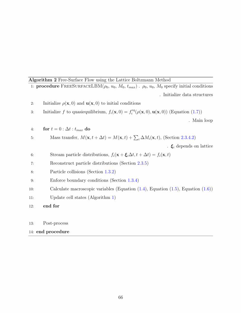
Algorithm 2 Free-Surface Flow using the Lattice Boltzmann Method1: procedure FreeSurfaceLBM(ρ0, u0, M0, tmax) . ρ0, u0, M0 specify initial conditions

. Initialize data structures

2: Initialize ρ(x, 0) and u(x, 0) to initial conditions

3: Initialize f to quasiequilibrium, fi(x, 0) = f eqi (ρ(x, 0),u(x, 0)) (Equation (1.7))

. Main loop

4: for t = 0 : ∆t : tmax do

5: Mass transfer, M(x, t+ ∆t) = M(x, t) +∑

i ∆Mi(x, t), (Section 2.3.4.2)

. ξi depends on lattice

6: Stream particle distributions, fi(x + ξi∆t, t+ ∆t) = fi(x, t)

7: Reconstruct particle distributions (Section 2.3.5)

8: Particle collisions (Section 1.3.2)

9: Enforce boundary conditions (Section 1.3.4)

10: Calculate macroscopic variables (Equation (1.4), Equation (1.5), Equation (1.6))

11: Update cell states (Algorithm 1)

12: end for

13: Post-process

14: end procedure

66

Figure 2.4: Example simulation used in primary cementing study. The black rectangles on

the left boundary represent notches protruding from the rock formation surface. The contours

are of the primary fluid (cement slurry) mass. The schematic on the right is courtesy of [1]

.

67

The simulations were carried out on a 50×500 lattice. For the mass inlet, a [38] velocity

boundary condition was used in conjuction with a constant mass boundary condition, i.e.

M(xj, t) = M0 = 1.0 for all xj along the inlet. This corresponded to a constant mass flow,

Min = M0u0, at inlet. For the outlet, mass was allowed to transfer out of the domain during

the mass transfer step such that fß(x + ξi∆t, t) = 0 in (2.1) for all x + ξi∆t that lie outside

of the domain on the other side of the mass outlet (i.e. the boundary condition at the outlet

is such that there is no backflow). All simulations were executed for 16000 time steps.

The different imperfect geometries that were considered at the rock formation surface

were: flow over a cavity that is 30% of the annulus width, “cav 30 × 1”; flow over a cavity

that is 60% of the annulus width, “cav 60×1”; flow over a square obstacle with sides that are

30% of the annulus width, “obs 30 × 1”; flow over two square obstacles with sides that are

30% of the annulus width, “obs 30× 2”; flow over a square obstacle with sides that are 60%

of the annulus width, “obs 60× 1”; flow over two square obstacles with sides that are 60% of

the annulus width, “obs 60× 2”; and flow over a rectangular obstacle with width that is 60%

of the annulus width and length that is four times the width, “obs 60 × L”. The wellbore

geometries that were considered herein are depicted in Figure 2.5.

In addition to wellbore geometry, different cement slurry material properties and cement

slurry flow rates were considered, which are characterized by the dimensionless Reynold’s

number, Re = ρULµp

, and Bingham number, Bn = τyL

µpU, of the flow, where L ≡ the width

of the annulus. A particular goal of the study was to investigate which Reynold’s numbers

and Bingham numbers were preferable for each geometry, and which Reynold’s numbers

and Bingham numbers performed well for all geometries. The dimensionless numbers were

68

Figure 2.5: Wellbore geometries considered in the study.

defined as follows, (Re,Bn) = (1.00, 4.00), (2.50, 0.00), (2.50, 1.00), (2.50, 10.0), (2.50, 25.0),

(5.00, 5.00), and (12.5, 2.0). Figure 2.6 shows the percentage of the wellbore annulus section

filled at the end of the cement simulation duration. The percent fill was calculated as:∑x∈X

ε(x, 16000)∑x∈X

1.0. (2.5)

Based upon Figure 2.6, some general statements can be made about what properties

of the cement slurry flow are preferable. For example, low yield stress, and consquently

low Bingham number flows (Bn ≤ 1.0), approximately completely filled the annulus for

every wellbore geometry considered. In addition, the negligible percentage of voids for the

(Re = 5.00, Bn = 5.00) and (Re = 12.5, Bn = 2.0) slurry flows suggests that a if the ratio

of Bn/Re is low, that the slurry flow will result in a low percentage of voids for cementing

a dry hole as is desired. As Bn/Re increases, it appears that, in certain cases and wellbore

geometries, the slurry flow tends to result in a larger percentage of voids (approximately 10%-

40%). What is interesting to note is that for slurry flows that resulted in a percentage of

69

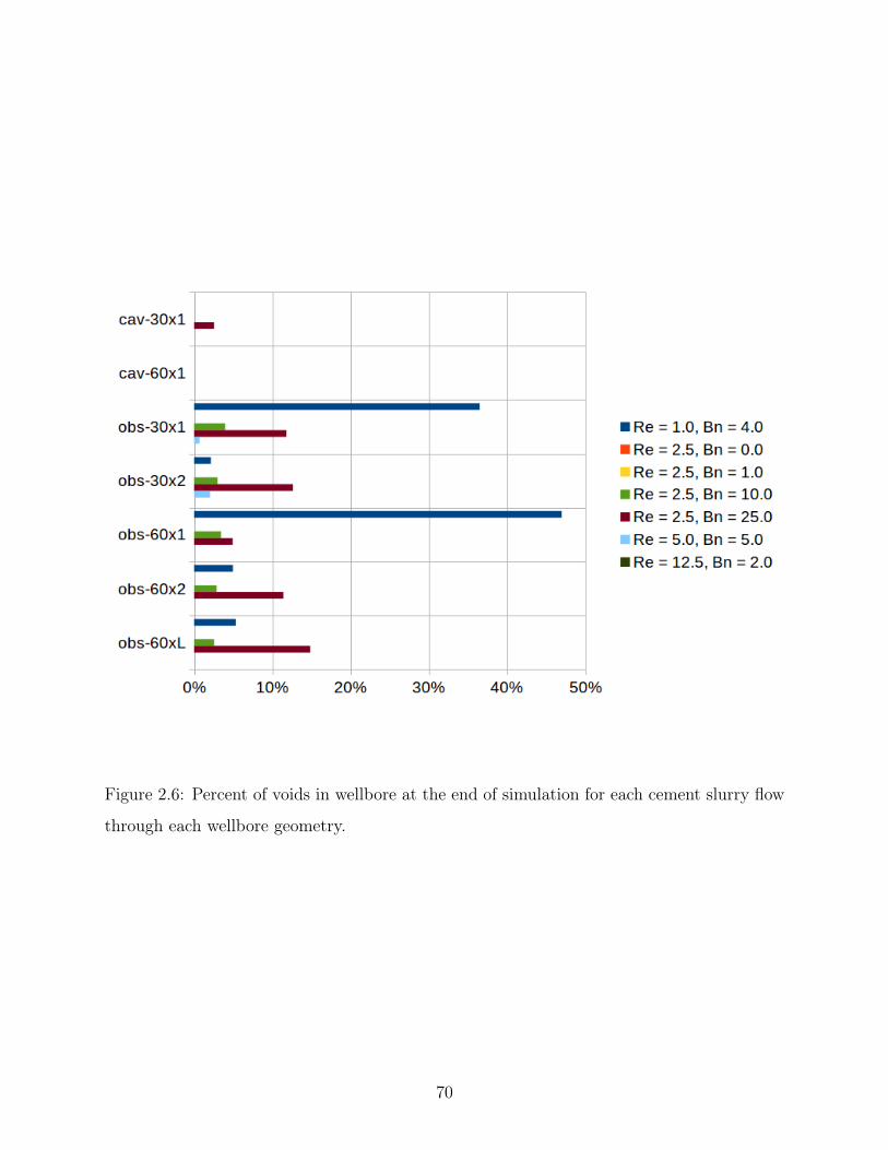
Figure 2.6: Percent of voids in wellbore at the end of simulation for each cement slurry flow

through each wellbore geometry.

70

voids greater than 3%, there was a lack of consistency across wellbore geometries in terms of

which slurry flow resulted in more voids and which slurry flow resulted in less, which suggests

that generalities cannot always be made and that computational methods are necessary for

understanding and designing slurry mixes for real-life wellbores.

2.5 CONCLUSIONS

An LBM model for simulating non-Newtonian and free-surface flow to represent cementing

dry annuli in oil and gas wellbores was presented. The model was then used to study how

different cement slurry flows, defined by different Reynold’s numbers and Bingham numbers,

would perform in different wellbore geometries. The results showed that in general, it is

preferable that the yield stress and Bn/Re ratio of the slurry flow be low. However, beyond

these considerations, it is not clear what slurry flow may be preferable for a given rock

formation geometry. The results suggest that computational methods are necessary for (a)

better understanding the mechanics of primary cementing and (b) for designing a cement mix

for a given wellbore. The lattice Boltzmann method extended for simulating non-Newtonian

and free-surface flow as presented in the current work has several properties that make it a

good candidate for such a design framework:

• LBM is well-suited for simulating non-Newtonian fluids because the strain-rate tensor is

computed local to each node and is second-order accurate [4, 39].

• LBM is well-suited for simulating multiphase multicomponent flow and free-surface flow

because it can handle complicated interface shapes between fluid phases and components.

• LBM is easily written in parallel and as hardware architectures shifts sequential to parallel

computing, it becomes increasingly important that code for simulating complex and

computationally expensive phenomena be written in parallel.

• The LBM no-slip boundary condition works well with complex geometries, such as those

that occur in realistic rock formation surfaces in drilled wellbores.

71

Future work would include developing a more physically realistic model. Primary ce-

menting can involve multiple phases and multiple components, namely the cement slurry, a

spacer fluid, and drilling mud. Possible future work would be make the model more general

so as to be capable of simulating multiphase multicomponent flow. In addition, a more

physically realistic model would simulate three-dimensional flow so as to be able to simulate

eccentric annuli and three-dimensional rock formation imperfections.

72

3.0 CONCLUSIONS

Various Lattice Boltzmann methods were investigated for their efficacy in simulating pri-

mary cementing. Although non-Newtonian fluid mechanics only represent a portion of the

challenges associated with simulating primary cementing, the fluid components that can be

present in primary cementing exhibit various non-Newtonian behaviors such as yield stress

or Bingham plastic behavior (e.g. cement slurry), power-law behavior (e.g. drilling mud),

among other non-Newtonian behaviors. In Chapter 1, the accuracy, stability, and efficiency

of Lattice Boltzmann models in simulating non-Newtonian fluid flow was investigated. Two

different benchmark problems were chosen for the study: Poiseuille flow, and lid-driven

square cavity flow, as Poiseuille flow is characterized by the development of velocity profiles

and lid-driven cavity flow is characterized by the development of vortices. Conclusions from

the study were presented in Section 1.5. In the context of studying the accuracy, stabil-

ity, and efficiency of Lattice Boltzmann models for simulating non-Newtonian flow, future

work would include investigating the effect of the choice of time step size and simulation

Mach number (as in [66]) on the convergence rate and accuracy of the results and LB meth-

ods presented in Section 1.4. In addition, possible future work could include investigating

other physical problems such as planar sudden expansion flow [5, 6, 8, 10], reentrant corner

flow [22, 23], and flow around a cylinder [7]. In the context of simulating wellbore cement-

ing, future work would include studying the accuracy, stability, and efficiency of Lattice

Boltzmann models for simulating the thixotropic and time-dependent behavior of cement

slurry [67].

In Chapter 2, the LBM algorithm for non-Newtonian flow is extended to simulate free

surface flow. The extended LBM model is then used to study wellbore cementing. Future

work for the wellbore cementing study would include developing a more physically realistic

73

model. Primary cementing can involve multiple phases and multiple components, namely

the cement slurry, a spacer fluid, and drilling mud. Possible future work would be make the

model more general so as to be capable of simulating multiphase multicomponent flow. In

addition, a more physically realistic model would simulate three-dimensional flow so as to

be able to simulate eccentric annuli and three-dimensional rock formation imperfections.

74

BIBLIOGRAPHY

[1] Introduction to cementing. http://www.drillingcourse.com/2015/12/introduction-to-cementing.html, 2015. Accessed: 2016-07-01.

[2] G Bohme. Non-newtonian fluid mechanics. series in applied mathematics and mechanics,1987.

[3] Chen-Hao Wang and Jeng-Rong Ho. A lattice boltzmann approach for the non-newtonian effect in the blood flow. Computers & Mathematics with Applications,62(1):75–86, 2011.

[4] T Krüger, F Varnik, and D Raabe. Second-order convergence of the deviatoric stress ten-sor in the standard bhatnagar-gross-krook lattice boltzmann method. Physical ReviewE, 82(2):025701, 2010.

[5] GH Tang, SB Wang, PX Ye, and WQ Tao. Bingham fluid simulation with the in-compressible lattice boltzmann model. Journal of Non-Newtonian Fluid Mechanics,166:145–151, 2011.

[6] Zhenhua Chai, Baochang Shi, Zhaoli Guo, and Fumei Rong. Multiple-relaxation-time lattice boltzmann model for generalized newtonian fluid flows. Journal of Non-Newtonian Fluid Mechanics, 166(5):332–342, 2011.

[7] Keivan Fallah, Morteza Khayat, Mohammad Hossein Borghei, Atena Ghaderi, andEhsan Fattahi. Multiple-relaxation-time lattice boltzmann simulation of non-newtonianflows past a rotating circular cylinder. Journal of Non-Newtonian Fluid Mechanics,177:1–14, 2012.

[8] SongGui Chen, QiCheng Sun, Feng Jin, and JianGuo Liu. Simulations of binghamplastic flows with the multiple-relaxation-time lattice boltzmann model. Science ChinaPhysics, Mechanics and Astronomy, 57:532–540, 2014.

[9] A Vikhansky. Lattice-boltzmann method for yield-stress liquids. Journal of Non-Newtonian Fluid Mechanics, 155:95–100, 2008.

[10] Chen-Hao Wang and Jeng-Rong Ho. Lattice boltzmann modeling of bingham plastics.Physica A: Statistical Mechanics and its Applications, 387:4740–4748, 2008.

75

http://www.drillingcourse.com/2015/12/introduction-to-cementing.html

http://www.drillingcourse.com/2015/12/introduction-to-cementing.html

[11] Liang Wang, Jianchun Mi, Xuhui Meng, and Zhaoli Guo. A localized mass-conservinglattice boltzmann approach for non-newtonian fluid flows. Communications in Compu-tational Physics, 17(04):908–924, 2015.

[12] J Boyd, James Buick, and S Green. A second-order accurate lattice boltzmann non-newtonian flow model. Journal of physics A: Mathematical and General, 39:14241–14247, 2006.

[13] Mahmud Ashrafizaadeh and Hani Bakhshaei. A comparison of non-newtonian models forlattice boltzmann blood flow simulations. Computers & Mathematics with Applications,58(5):1045–1054, 2009.

[14] James D Sterling and Shiyi Chen. Stability analysis of lattice boltzmann methods. arXivpreprint comp-gas/9306001, 1993.

[15] James D Sterling and Shiyi Chen. Stability analysis of lattice boltzmann methods.Journal of Computational Physics, 123(1):196–206, 1996.

[16] Saleh Bawazeer. Stability and accuracy of lattice boltzmann method. 2013.

[17] Pierre Lallemand and Li-Shi Luo. Theory of the lattice boltzmann method: Dispersion,dissipation, isotropy, galilean invariance, and stability. Physical Review E, 61:6546–6542,2000.

[18] Oldřich Švec, Jan Skoček, Henrik Stang, John Forbes Olesen, and Peter Noe Poulsen.Flow simulation of fiber reinforced self compacting concrete using lattice boltzmannmethod. 2011.

[19] Oldřich Švec, Jan Skoček, Henrik Stang, Mette R Geiker, and Nicolas Roussel. Free sur-face flow of a suspension of rigid particles in a non-newtonian fluid: A lattice boltzmannapproach. Journal of Non-Newtonian Fluid Mechanics, 179:32–42, 2012.

[20] Yanlong Zhao, Zhiming Wang, Quanshu Zeng, Jiangtao Li, and Xiao Guo. Latticeboltzmann simulation for steady displacement interface in cementing horizontal wellswith eccentric annuli. Journal of Petroleum Science and Engineering, 145:213–221,2016.

[21] Jonas Latt. Hydrodynamic limit of lattice Boltzmann equations. PhD thesis, Universityof Geneva, 2007.

[22] Susana Gabbanelli, German Drazer, and Joel Koplik. Lattice boltzmann method fornon-newtonian (power-law) fluids. Physical Review E, 72(4):046312, 2005.

[23] M Yoshino, Y Hotta, T Hirozane, and M Endo. A numerical method for incompressiblenon-newtonian fluid flows based on the lattice boltzmann method. Journal of non-newtonian fluid mechanics, 147:69–78, 2007.

76

[24] Dominique d’Humieres. Generalized lattice-boltzmann equations. Rarefied gasdynamics- Theory and simulations, pages 450–458, 1994.

[25] RA Brownlee, Alexander N Gorban, and Jeremy Levesley. Stabilization of the lat-tice boltzmann method using the ehrenfests’ coarse-graining idea. Physical Review E,74(3):037703, 2006.

[26] RA Brownlee, Alexander N Gorban, and Jeremy Levesley. Stability and stabilization ofthe lattice boltzmann method. Physical Review E, 75(3):036711, 2007.

[27] RA Brownlee, Alexander N Gorban, and Jeremy Levesley. Nonequilibrium entropylimiters in lattice boltzmann methods. Physica A: Statistical Mechanics and its Appli-cations, 387(2):385–406, 2008.

[28] Dave Packwood. Entropy balance and dispersive oscillations in lattice boltzmann mod-els. Physical Review E, 80(6):067701, 2009.

[29] Alexander N Gorban and DAVID J Packwood. Enhancement of the stability of latticeboltzmann methods by dissipation control. Physica A: Statistical Mechanics and itsApplications, 414:285–299, 2014.

[30] Shiyi Chen and Gary D Doolen. Lattice boltzmann method for fluid flows. Annualreview of fluid mechanics, 30:329–364, 1998.

[31] Sauro Succi. The Lattice Boltzmann Equation for Fluid Dynamics and Beyond. OxfordUniversity Press, New York, 2001.

[32] Carlo Cercignani. Mathematical methods in kinetic theory. Springer, 1990.

[33] P. Bhatnagar, E. Gross, and M. Krook. A model for collisional processes in gases i:small amplitude processes in charged and neutral one-component system. Phys. Rev.,94, 1954.

[34] Dieter A Wolf-Gladrow. Lattice-gas cellular automata and lattice Boltzmann models:An Introduction. Springer Science & Business Media, 2000.

[35] Paul J Dellar. Incompressible limits of lattice boltzmann equations using multiple re-laxation times. Journal of Computational Physics, 190(2):351–370, 2003.

[36] Dominique d’Humières. Multiple–relaxation–time lattice boltzmann models in threedimensions. Philosophical Transactions of the Royal Society of London A: Mathematical,Physical and Engineering Sciences, 360(1792):437–451, 2002.

[37] Matthew Grasinger, Zichang Li, Alex Vuotto, John Brigham, Anthony Iannacchione,Julie Vandenbossche, et al. Simulation of cement slurry flow to assess the potential forvoids and channels in wellbore cementing processes. In SPE Eastern Regional Meeting.Society of Petroleum Engineers, 2015.

77

[38] Qisu Zou and Xiaoyi He. On pressure and velocity boundary conditions for the latticeboltzmann bgk model. Physics of Fluids (1994-present), 9:1591–1598, 1997.

[39] Timm Krüger, Fathollah Varnik, and Dierk Raabe. Shear stress in lattice boltzmannsimulations. Physical Review E, 79:046704, 2009.

[40] Eugene Cook Bingham. Fluidity and plasticity, volume 2. McGraw-Hill Book Compny,Incorporated, 1922.

[41] Tasos C Papanastasiou. Flows of materials with yield. Journal of Rheology (1978-present), 31:385–404, 1987.

[42] Qiuxiang Li, Ning Hong, Baochang Shi, and Zhenhua Chai. Simulation of power-lawfluid flows in two-dimensional square cavity using multi-relaxation-time lattice boltz-mann method. Communications in Computational Physics, 15(01):265–284, 2014.

[43] Alexandros Syrakos, Georgios C Georgiou, and Andreas N Alexandrou. Performanceof the finite volume method in solving regularised bingham flows: Inertia effects in thelid-driven cavity flow. Journal of Non-Newtonian Fluid Mechanics, 208:88–107, 2014.

[44] Michael J Economides. 1 implications of cementing on well performance. Developmentsin Petroleum Science, 28:1–6, 1990.

[45] PB Jackson, CE Murphey, et al. Effect of casing pressure on gas flow through a sheathof set cement. In SPE/IADC drilling conference. Society of Petroleum Engineers, 1993.

[46] KJ Goodwin, RJ Crook, et al. Cement sheath stress failure. SPE Drilling Engineering,7(04):291–296, 1992.

[47] Maurice B Dusseault, Richard E Jackson, and Daniel Macdonald. Towards a road mapfor mitigating the rates and occurrences of long-term wellbore leakage. University ofWaterloo and Geofirma Engineering LTD, 2014.

[48] Zichang Li, Julie Vandenbossche, Anthony Iannacchione, John Brigham, BarbaraKutchko, et al. Theory-based review of limitations with static gel strength in ce-ment/matrix characterization. SPE Drilling & Completion, 2016.

[49] SH Bittleston, J Ferguson, and IA Frigaard. Mud removal and cement placement duringprimary cementing of an oil well–laminar non-newtonian displacements in an eccentricannular hele-shaw cell. Journal of Engineering Mathematics, 2:229–253, 2002.

[50] PR Cheung and Robert M Beirute. Gas flow in cements. Journal of petroleum technology,06:1041–1048, 1985.

[51] Dennis C Levine, Eugene W Thomas, HP Bezner, and Glen C Tolle. Annular gas flowafter cementing: a look at practical solutions. Society of Petroleum Engineers, 1979.

78

[52] RB Stewart and Schouten FC. Gas invasion and migration in cemented annuli: Causesand cures. SPE drilling engineering, 01:77–82, 1988.

[53] Soran Talabani, GA Chukwu, and DG Hatzignatiou. A unique experimental studyreveals how to prevent gas migration in a cemented annulus. Society of PetroleumEngineers, 1993.

[54] Muhammad Zulqarnain. Simulations of the primary cement placement in annular ge-ometries during well completion using computational fluid dynamics (cfd). Technicalreport, Baton Rouge, 2012.

[55] Robert M Beirute and Raymond W Flumerfelt. Mechanics of the displacement processof drilling muds by cement slurries using an accurate rheological model. Society ofPetroleum Engineers, 1977.

[56] Daniel T Thorne and C Michael. Lattice Boltzmann modeling: An introduction forgeoscientists and engineers. Springer, 2006.

[57] C Ferraris, F De Larrard, and N Martys. Fresh concrete rheology: recent developments.Materials Science of Concrete VI, Amer. Cer. Soc. Ed. S. Mindess, J. Skalny, pages215–241, 2001.

[58] Chiara F Ferraris and François de Larrard. Testing and modelling of fresh concreterheology. US Department of Commerce, Technology Administration, National Instituteof Standards and Technology, 1998.

[59] Geoffrey Howarth Tattersall. Workability and quality control of concrete. CRC Press,2003.

[60] Nicolas Roussel, Mette R Geiker, Frédéric Dufour, Lars N Thrane, and Peter Szabo.Computational modeling of concrete flow: General overview. Cement and Concreteresearch, 37:1298–1307, 2007.

[61] Nicolas Roussel, Annika Gram, Massimiliano Cremonesi, Liberato Ferrara, Knut Kren-zer, Viktor Mechtcherine, Sergiy Shyshko, Jan Skocec, Jon Spangenberg, Oldrich Svec,et al. Numerical simulations of concrete flow: A benchmark comparison. Cement andConcrete Research, 2015.

[62] Zhenhua Chai, Baochang Shi, Zhaoli Guo, and Fumei Rong. Multiple-relaxation-time lattice boltzmann model for generalized newtonian fluid flows. Journal of Non-Newtonian Fluid Mechanics, 5:332–342, 2011.

[63] Timothy Nigel Phillips and Gareth Wyn Roberts. Lattice boltzmann models for non-newtonian flows. IMA journal of applied mathematics, 76(5):790–816, 2011.

[64] Carolin Körner, Michael Thies, Torsten Hofmann, Nils Thürey, and Ulrich Rüde. Latticeboltzmann model for free surface flow for modeling foaming. Journal of StatisticalPhysics, 121:179–196, 2005.

79

[65] Nils Thürey, C Körner, and U Rüde. Interactive free surface fluids with the latticeboltzmann method. Technical Report05-4. University of Erlangen-Nuremberg, Germany,2005.

[66] Daniel Conrad, Andreas Schneider, and Martin Böhle. Accuracy of non-newtonianlattice boltzmann simulations. Journal of Computational Physics, 301:218–229, 2015.

[67] Nicolas Roussel. Steady and transient flow behaviour of fresh cement pastes. Cementand concrete research, 35:1656–1664, 2005.

80

Evaluating the Capabilities of the Lattice Boltzmann Method...

Documents

Transcript of Evaluating the Capabilities of the Lattice Boltzmann Method...