1

Evaluating Temporal Robustness ofMobile Networks

Salvatore Scellato∗, Ilias Leontiadis∗, Cecilia Mascolo∗, Prithwish Basu†, Murtaza Zafer‡∗Computer Laboratory, University of Cambridge, UK

†Raytheon BBN Technologies, MA, USA‡IBM T. J. Watson Research, NY, USA

Abstract—The application of complex network models to communication systems has led to several important results: nonetheless,previous research has often neglected to take into account their temporal properties, which in many real scenarios play a pivotal role.At the same time, network robustness has come extensively under scrutiny. Understanding whether networked systems can undergostructural damage and yet perform efficiently is crucial to both their protection against failures and to the design of new applications. Inspite of this, it is still unclear what type of resilience we may expect in a network which continuously changes over time.In this work we present the first attempt to define the concept of temporal network robustness: we describe a measure of networkrobustness for time-varying networks and we show how it performs on different classes of random models by means of analytical andnumerical evaluation. Finally, we report a case study on a real-world scenario, an opportunistic vehicular system of about 500 taxicabs,highlighting the importance of time in the evaluation of robustness. Particularly, we show how static approximation can wrongly indicatehigh robustness of fragile networks when adopted in mobile time-varying networks, while a temporal approach captures more accuratelythe system performance.

Index Terms—Mobile networks, temporal networks, network robustness.

F

1 INTRODUCTION

The study of real-world communication systems bymeans of complex network models has provided in-sightful results and has vastly expanded our knowl-edge on how single entities create connections andhow these connections are used for communication or,more generally, interaction [1]. Statistical network mod-els such as the Erdos Renyi random graph [2] and thescale-free networks generated by preferential-attachmentmechanisms [3] have been largely exploited to studyand understand real-world systems. While the formermodel embodies networks whose nodes are statisticallyindistinguishable, resulting in fairly homogenoues prop-erties, scale-free networks exhbit heterogeneous nodeproperties, with the vast majority of nodes having afew connections and a small minority of hubs having adisproportionately large number of links. The differentproperties present in these two families of models areable to capture a vast range of real-world systems. Inparticular, technological networks such as the Internetand the World Wide Web have been under scrutinyin terms of structure and dynamic behavior [4], [5].More recently, with the widespread adoption of mobileand opportunistic networks, it has become importantto develop new analytical tools to keep into accountnetwork dynamics over time [6], [7] and how this affectsphenomena such as information propagation [8], [9].

An earlier initial version of this work appeared in Proceedings of IEEE Info-com 2011, Miniconference track, with the title “Understanding Robustnessof Mobile Networks through Temporal Network Measures”.

Results have shown that time correlations and relativetemporal ordering of connection events among nodescannot be neglected, otherwise the performance of agiven system can be greatly overestimated [10], [11].

At the same time, the problem of understandingwhether real systems can sustain substantial damage andstill maintain acceptable performance has been exten-sively addressed [12], [13]. Various measures of networkrobustness have been defined and investigated for sev-eral classes of networks, evaluating how different systemcan be more or less resilient against random errors ortargeted attacks thanks to their underlying structuralproperties [14], [15].

Nonetheless, it is still unclear how to approach thestudy of robustness of networks by taking into accounttheir time-varying nature: by adopting a static represen-tation of a temporal network, important features whichimpact the actual performance might be missed. Thus,it becomes important to develop a robustness metricwhich takes into account the temporal dimension andgives insights on how a mobile network is affected bydamage or change. Particularly, the fact that links are notalways active means that information spreading can bedelayed or even stopped and that relative ordering in timeof connection events may affect the creation of temporal pathsin mobile networks.

Our main goal is to design a novel framework for theanalysis of robustness in mobile time-varying networks.We adopt temporal network metrics [10] to quantify net-work performance and define a measure of robustnessagainst generic network damages. At first, we study its

2

performance on random network models to understandits properties; then we apply our method to study a realmobile network, describing how temporal robustnessgives a more accurate evaluation of system resiliencethan static approaches.

Our contributions can be summarized as follows:• We describe the use of temporal network metrics

such as temporal distance to estimate the currentnetwork connectivity taking temporal variabilityinto account. We define temporal network robustness(Section 2), a novel measure which quantifies howthe communication of a given time-varying networkis affected by damage.

• We provide an analytical computation of temporalmetrics on a temporal version of the Erdos Renyi(ER) random graph model (Section 3) and we eval-uate through numerical simulation both a Markov-based link connectivity model, which provides time-correlations, and two random mobility models,which introduce space-correlations (Section 4).

• We show how, unlike what has been demonstrated withstatic measures, temporal networks do not exhibit sharpbreakdowns but instead fail gracefully when they aresubjected to failures. The temporal dimension is ableto capture the evolution dynamics, exposing the factthat time allows to create temporal paths acrossotherwise disconnected portions of the network.

• We investigate the usefulness of our approach tocharacterize a real communication system, an op-portunistic vehicular network simulated with realmobility traces of about 500 taxis in the San Fran-cisco Area (Section 5): we show that the robustnessevaluation based on static network analysis is too opti-mistic in real scenarios, since it greatly overestimateshow resilient a mobile system really is, withoutgiving reliable measures.

We discuss some implications of our findings for thedesign of new systems and applications (Section 6).Finally, we review related results on this topic (Section 8)and we conclude the paper (Section 9).

2 TEMPORAL ROBUSTNESS

In this section we will review some basic metrics fortemporal networks and describe how these measures canbe adopted to quantitatively define temporal networkrobustness.

2.1 Network Robustness

The study of robustness of complex networks has mainlyfocused on describing how a given performance metricof the network is affected when nodes are removedaccording to a certain rule. The underlying assumptionis that the absence or malfunctioning of some nodes willcause the removal of their edges and, thus, some pathswill become longer, increasing the distances between theremaining nodes, or completely disappear, resulting in

the loss of connectivity in the whole system. The per-formance measures previously adopted include the net-work diameter [12], the size of the giant component [12],[14] and the average inverse geodesic length [14], [15].Moreover, the strategies used to choose which nodes areto be removed can be divided in two broad categories:random failures, where every node has the same prob-ability of being removed, and targeted attacks, wherenodes are ranked according to a performance metric andthen accordingly removed [14].

In this work we will study the problem of definingand analyzing robustness in evolving networks: as aconsequence, we need to use a performance metric whichincludes the temporal dimension in its definition. At the sametime, we focus on the first strategy of node removal:we consider random and independent failures for everynode and we evaluate how the system tolerates increas-ing level of malfunctioning nodes.

2.2 Temporal Network Metrics

In networks where nodes can connect with a largenumber of other nodes over time (e.g., mobile and peerto peer networks) time ordering of events is important.Traditional approaches that aggregate links over timealways overestimate network connectivity, which meansthat some paths that seem to be present are in reality notpresent due to the actual ordering of the links over time.Hence, in this section we describe the notion of temporalgraph we use to model mobile networks [10], [11].

Temporal graph: A temporal graph is a graph G(t) =(V (t), E(t)) where V (t) is the set of nodes at time tand E(t) is the set of edges at time t. We assume that|V (t)| = N , thus nodes cannot be added from the graph,while nodes can be removed by disconnecting them fromthe rest of the network. Furthermore, we treat time asa discrete entity and we create a sequence of graphsG(t1), . . . G(t2) by adopting an appropriate resolutiontime.

Temporal distance: Then, given two nodes i and jwe can define a temporal path pij(t1, t2) between themin the time window [t1, t2]. The length of a temporalpath is defined as the amount of time steps it takesto spread information from node i to node j on thatparticular path. This value is always a positive integer.As a consequence, we can define the shortest temporaldistance dij(t1, t2) as the smallest length among all thetemporal paths between nodes i and j in time window[t1, t2]. For example, if a message sent by node A isreceived by node B at time td, then dAB = td − t1. Ifthere is no temporal path between i and j in [t1, t2], theirdistance can be considered infinite, i.e. dij(t1, t2) = ∞.The average temporal distance L(t1, t2) of a given temporalgraph G during a time window [t1, t2] is defined as:

L(t1, t2) =1

N(N − 1)

∑i,j

dij(t1, t2) (1)

3

This quantity is not well defined when some pairs ofnodes are not temporally connected. As a consequence,another metric has been introduced.

Temporal efficiency: We can define the temporal globalefficiency E(t1, t2) of a given temporal graph G

E(t1, t2) =1

N(N − 1)

∑i,j

1

dij(t1, t2)(2)

This value is not affected by disconnected pairs of nodes,because their contribution to the efficiency is computedas zero. Network efficiency is normalized between 0 and1 and it does not depend on the size of network, hence,it can be adopted to compare graphs with differentsizes. The concept of network efficiency was originallyintroduced for static graphs explicitly to cope with dis-connected couples and it measures how well nodes incan communicate [16].

Since a temporal graph is continuously evolving, wecan evaluate how temporal efficiency changes over timeby considering a value τ and evaluating EG(t) as therelative temporal efficiency of the temporal graph in thetime window [t − τ, t]. The effect of τ is to effectivelyimpose an upper bound on the temporal distances, asall paths longer than τ simply do not exist. As a conse-quence, τ should be chosen so that any communicationwhose delay is longer than τ itself can be ignored.Similarly, LG(t) is computed as the average temporaldistance in [t − τ, t]. If the properties of the temporalgraph are stationary, we expect these values to reach asteady value as time progresses. For instance, a temporalgraph whose links are evolving according to an ergodicrandom process will exhibit stationary behavior, whilea temporal graph whose evolution is ruled by a time-dependent process might not reach stationarity at all.In practice, a temporal graph with stationary propertiesmight reach an equilibrium point where temporal effi-ciency is fluctuating around its average value, while thismight not be valid for non-stationary temporal graphs.

0 50 100 150 200 250 300

t

0.00

0.05

0.10

0.15

0.20

0.25

EG

(t)

Fig. 1. Temporal efficiency in a time-varying network: att = 150 20% of the nodes are removed. The relative dropin efficiency after the damage can be used to quantify therobustness of the network.

2.3 Temporal Robustness MetricGiven a temporal graph G, we define a damage D asany structural modification on it and we define GD asthe graph resulting by the effect of the damage D onG. A damage may be the deactivation of some nodesor the removal of some edges at a particular time tD.Because of damage D, some temporal shortest paths willbe longer or will not exist any more, thus, we expectthat the temporal efficiency will eventually reach a newsteady value EGD

≤ EG. It is important to evaluate thenew value of the temporal efficiency on a new temporalgraph which still contains the deactivated nodes, inorder to obtain a decrease in efficiency. Otherwise, wemight obtain a smaller temporal graph which is moreefficient than the original graph, although it has lostmuch of its structure. Hence, we do not consider highlydynamic systems where nodes can be constantly addedor removed. Instead, we focus on evaluating the servicedegradation in a more controlled environment whereonly a number of existing nodes could fail.

We define the loss in efficiency ∆E(G,D) caused bythe damage D on the temporal graph G as ∆E(G,D) =EG − EGD

. Finally, we define the temporal robustnessRG(D) of the temporal graph against the damage D as

RG(D) = 1− ∆E(G,D)

EG=EGD

EG(3)

This value is normalized between 0 and 1 and it mea-sures the relative loss of efficiency caused by the damage:if the damage does not impact the efficiency of the graph(EGD

= EG) then its robustness is 1, while if the damagedestroys the efficiency of the graph (EGD

= 0) the ro-bustness drops to 0. Temporal efficiency is a particularlysuitable metric to study temporal network robustnessas it denotes both longer temporal paths and the lackof paths among temporally disconnected nodes at thesame time. Nonetheless, other metrics have been usedto assess robustness in static systems: for instance, therecould be scenarios where fast communication with smalldelays can be more important than global connectivity,thus other measures can be adopted. Provided that thesemeasures can be extended to the temporal case, they canbe easily integrated in our framework.

For example, as we see in Figure 1 for a randomtemporal network (see Section 3 for more details), a dam-age which affects a fraction of the nodes in a temporalgraph will result in a drop of the temporal efficiency.By measuring the amount of lost efficiency we canquantify the robustness of the network to that particulardamage. Moreover, by normalizing the efficiency dropwith respect to the original efficiency of the network,we can compare the robustness of systems with differentproperties and sizes.

3 THEORETICAL ANALYSIS

In this section we analytically investigate how temporalmetrics and temporal robustness evaluate on a random

4

model of a temporal network, namely a generalizationof the Erdos Renyi random graph [2].

3.1 Temporal Random Network Model

An Erdos Renyi (ER) random graph with N nodes andparameter p is created by independently including eachpossible edge in the graph with probability p, thusresulting in an expected number of edges K = pN(N−1)

2 ,and it is denoted as G(N, p) [2]. This model has beensuccessfully adopted to represent a simple random net-work, where only the density of links is fixed and allthe rest is randomized. We generalize this model to thetemporal case by creating a sequence of T ER randomgraphs G(N, p) and we denote the resulting temporalgraph as G(N, p, T ).

The simplicity of this model allows a theoretical anal-ysis and the computation of its temporal metrics as afunction of its parameters N , p and T . More precisely,we are interested in this question: if the flooding of amessage initiates from a random node at time t = 0, atwhich time step will other nodes receive it? This problemhas already been addressed by researchers studying epi-demic dissemination in mobile systems [17]: nonetheless,their temporal analysis of message spreading usuallyexploits either mean-field approximation to study theirbehavior in the limit of large systems [18]. Some at-tempts have also focused on providing tight bounds onthe speed of information dissemination on Markoviantime-varying graphs [19]. These solutions provide goodestimation of steady state behavior of the system, butcan be misleading when they are used to analyze thetransient behavior of the first steps of the dissemination.Instead, we are interested in the exact solution of thismodel in the case of a finite system with N nodes andwith discrete treatment of time, since we need to focuson the exact temporal values of message delay also forthe transient phase. As a consequence, we cannot usecontinuous mean-field formulation and we instead solvethe problem by modeling it as a discrete state randomprocess.

Let Nt be the random discrete process that counts thenumber of nodes which have received the message attime t: our aim is to compute the probability distributionof this random process for any given time 0 ≤ t ≤ T .In the following we use P (E) to denote the probabilitythat event E occurs. In addition, we will treat the case ofan arbitrary given node, without specifying any index,as in our case different nodes are statistically indistin-guishable. We will make use of the following lemma tocompute the probability distribution of Nt for 0 ≤ t ≤ T :

Lemma 1. The probability pm that a single node without themessage receives it in a time step when m other nodes alreadyhave it is given by pm = 1− (1− p)m.

Proof: A node without the message will receive itin a given time step if at least one of the other m nodeswith the message activates a link with it. Since every link

10−4 10−3 10−2 10−1 100

p

0

10

20

30

40

50

60

70

80

LG

SimulationTheoretical

(a) Average temporal length

10−4 10−3 10−2 10−1 100

p

0.0

0.2

0.4

0.6

0.8

1.0

CG

SimulationTheoretical

(b) Temporal connected couples

10−4 10−3 10−2 10−1 100

p

0.0

0.1

0.2

0.3

0.4

0.5

0.6

0.7

0.8

0.9

EG

SimulationTheoretical

(c) Temporal efficiency

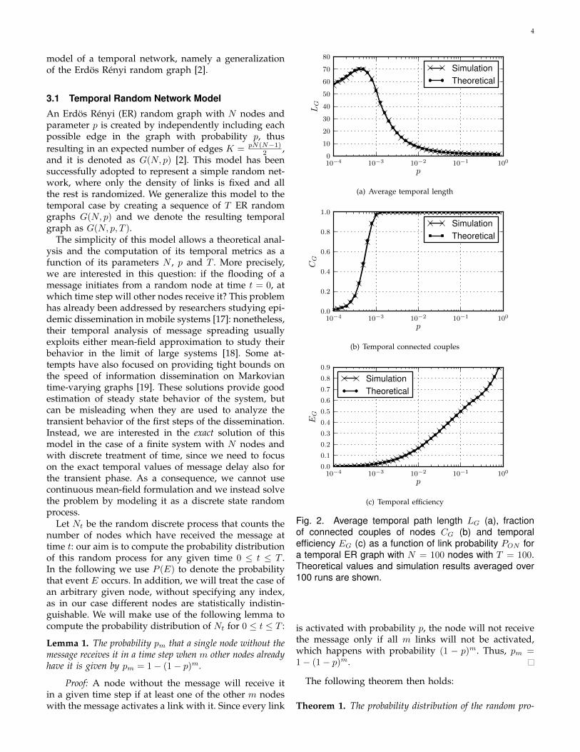
Fig. 2. Average temporal path length LG (a), fractionof connected couples of nodes CG (b) and temporalefficiency EG (c) as a function of link probability PON fora temporal ER graph with N = 100 nodes with T = 100.Theoretical values and simulation results averaged over100 runs are shown.

is activated with probability p, the node will not receivethe message only if all m links will not be activated,which happens with probability (1 − p)m. Thus, pm =1− (1− p)m.

The following theorem then holds:

Theorem 1. The probability distribution of the random pro-

5

cess Nt is:

P (Nt+1 = k) =

k∑m=1

(N −mk −m

)pk−mm (1− pm)N−kP (Nt = m)

(4)

with the initial condition P (N0 = 1) = 1.

Proof: We have an initial condition with only 1node with the message at time t = 0, the sender, soP (N0 = 1) = 1. In addition, the number of nodes reachedby the message can only increase with time. Then, theprobability distribution of Nt+1 is defined as a functionof the probability distribution of Nt:

P (Nt+1 = k) =

k∑m=1

P (Nt+1 = k|Nt = m)P (Nt = m)

=

k∑m=1

P (Mk−m|Nt = m)P (Nt = m)

where Mk−m is the event that k − m new nodes arereached by the message when there are already m nodeswith the message in the system. The probability that thisevent happens does not depend on time t but only onm. When there are N − m nodes that can be reachedby the message, each of them will get the message withprobability pm. Then, Eq.(5) can be expressed in termsof a binomial distribution with parameter pm for everyvalue of m, giving Eq. (4).

P (Nt+1 = k) =

k∑m=1

P (Mk−m|Nt = m)P (Nt = m) =

P (Nt+1 = k) =

k∑m=1

(N −mk −m

)pk−mm (1− pm)N−kP (Nt = m)

As a consequence, we have the following result on theprobability of a certain message delay:

Corollary 1. The probability Rt that a node has received themessage after t steps is given by

Rt =

N∑k=1

k − 1

N − 1P (Nt = k) (5)

Proof: The result comes from the fact that whenNt = k any node different than the source, and chosen atrandom, has the message with uniform probability k−1

N−1 .

Since P (N0 = 1) = 1, then R0 = 0. Instead, as t in-creases the probability of receiving the message increasesas well. In particular, if l is the message delay of a givennode, then Rt = P (l ≤ t),

Corollary 2. The probability that a node is reached by themessage exactly at time t is

dt = P (l = t) = P (l ≤ t)− P (l ≤ t− 1) = Rt −Rt−1 (6)

Proof: If a node is reached by time t then either it isreached exactly at time t or it is was already reached bytime t− 1, giving Rt = dt +Rt−1.

This derivation gives us the exact probability distribu-tion dt of temporal distances in G(N, p, T ), which enablesus to compute temporal metrics. The final fraction CG ofnodes reached by a temporal path before t = T is givenby Rt, whereas the expected average temporal lengthLG

1 and temporal efficiency EG can be computed usingthe probability distribution dt:

CG = RT (7)

LG =1

CG

T∑t=1

tdt (8)

EG =

T∑t=1

1

tdt (9)

3.2 Temporal MetricsIn order to validate our results, we simulate this modelfor various values of p and we compute temporal ef-ficiency EG(t) with N = 100 nodes for 500 time stepswith a time window of τ = 100, computing the averageefficiency value over the last τ steps. We also evaluatethe average temporal length LG and the fraction ofconnected couples of nodes CG. We then compare theseresults with the analytical solution of G(N, p, τ) for thesame values of p. As we see in Figure 2, theoreticalderivation and numerical simulation are in perfect agree-ment. We also note that as the probability p increasesboth temporal efficiency and the number of connectedcouples increases. Instead, the average temporal distanceLG reaches a maximum value and then decreases as weincrease p (Figure 2(a)). This is due to the fact that for lowvalues of p not all the couples of nodes can be connectedby a temporal path in the sequence of T graphs: thus,by increasing p, more and more couples can be reachedbut with longer paths. As soon as total connectivity isreached (Figure 2(b)), so that there exists a temporalpath between any pair of nodes, larger values of p givea decreasing temporal distance LG. This demonstrateshow temporal efficiency EG is a better measure thantemporal distance: since it is not affected by partialtemporal connectivity it gives a clear indication of thetemporal performance of the network (Figure 2(c)).

Furthermore, we note that there is no evidence of sharptransition from a disconnected to a connected temporal graph,since as we increase p the fraction of connected couplesCG smoothly increases from 0 to 1. This effect is dueto the temporal dimension: in this model, no matterhow small p is, the temporal graph will be eventuallyconnected as T → ∞ as long as there is a non-zeroprobability that each link is present. On the other hand,in the static case a ER random graph will experience a

1. This is computed only on the connected couples, so CG is theconditional probability that a node is reached by a temporal path.

6

sharp transition and will be connected, on average, onlywhen p approaches lnN

N [2].Finally, we investigate the impact of parameters N

and T on the temporal metrics by analyzing temporalefficiency EG. Figure 3(a) reports the relation betweenEG and probability p for two models with size N = 100and N = 1000. A larger number of nodes results inhigher efficiency for the same value of p, since thenumber of potential links in the model increases as N2

and thus there are many more potential paths to beused to connect nodes. Instead, we see in Figure 3(b)that the length of the interval T is not affecting theresults: as long as T is large enough to allow the creationof the temporal paths, increasing it will not make anydifference. The influence of T on temporal efficiencydecreases as T increases: all potential paths that arelonger than T are effectively removed, but longer pathscontribute less and less to temporal efficiency. As aresult, when temporal efficiency is evaluated empiricallyby using a sliding window τ a value large enough tolet temporal paths be created needs to be used. Largervalues will not make any difference and, instead, theymight slow down the computation.

3.3 Temporal RobustnessWe evaluate the temporal robustness of the temporalER model by directly computing the temporal efficiencyfor a normal network and for a damaged network. Wemodel a damage as a random failure of the nodes in thesystem by independently deactivating with probabilityPERR each node. As a result, an expected number ofND = NPERR nodes will be deactivated, thus notparticipating in any more communication. The damagecan be then entirely quantified by the probability of errorPERR: in this work we only consider independent andidentically distributed error probabilities, even thoughour framework can be extended to address also morecomplex cases with correlated errors. Thus, we investi-gate this model to understand how the temporal robust-ness measure behaves across systems with different sizeand different efficiency.

As reported in Figure 4, temporal robustness showsthat this random model fails smoothly as we increasethe fraction of removed nodes, without any sudden dis-ruption for any value of PERR. This is a main differencewith respect to what happens in the static case: for astatic ER random graph be a critical value of PERR

which causes a breakdown of the network in severaldisconnected components may exist [12]. This is not truefor temporal robustness, as new paths can still appearafter the damage as the network rearranges its con-nections. Time provides more redundancy and, hence,more resilience. Moreover, we also note that temporalrobustness does not depend on system size: since itis normalized with respect to the value of temporalefficiency before the damage, it depends only on therelative drop in efficiency, not on the absolute values ofthe metric.

10−4 10−3 10−2 10−1 100

p

0.0

0.1

0.2

0.3

0.4

0.5

0.6

0.7

0.8

0.9

EG

1001000

(a) Effect of N

10−4 10−3 10−2 10−1 100

p

0.0

0.1

0.2

0.3

0.4

0.5

0.6

0.7

0.8

0.9

EG

10.020.050.0100.0

(b) Effect of τ

Fig. 3. Temporal efficiency EG with τ = 100 and for twosystems with N = 100 and N = 1000 nodes (Figure 3(a)):larger systems result in higher efficiency values for thesame p, except for higher values of p. Temporal efficiencyEG as a function of probability of link presence p for dif-ferent values of τ for a system with N = 100 (Figure 3(b)):different values of τ result in similar values of temporalefficiency.

4 NUMERICAL EVALUATION

After the theoretical investigation of temporal robust-ness on a simplistic random model, we proceed tothe evaluation of this metric on more complex modelswhich introduce correlations in the temporal graph, withthe aim of investigating how these correlations impacttemporal network robustness. In this section we presenta numerical analysis of temporal metrics and robustnessfor two different classes of random temporal networks,evaluating their resilience against random errors.

4.1 Temporal Network Models4.1.1 Markov-based Temporal Network ModelThe temporal ER network model does not provide tem-poral correlations between consecutive graphs in the se-quence. We now consider a model where link evolutionis described by a Markov process, thus enabling memoryeffects in network dynamics [20].

7

0.0 0.2 0.4 0.6 0.8 1.0

PERR

0.0

0.2

0.4

0.6

0.8

1.0RG

1.0e-041.0e-031.0e-021.0e-01

(a) N = 100

0.0 0.2 0.4 0.6 0.8 1.0

PERR

0.0

0.2

0.4

0.6

0.8

1.0

RG

1.0e-041.0e-031.0e-021.0e-01

(b) N = 1000

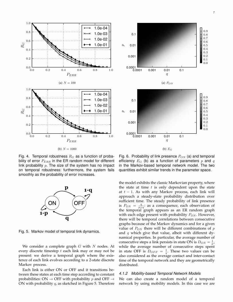
Fig. 4. Temporal robustness RG as a function of proba-bility of error PERR in the ER random model for differentlink probability p. The size of the system has no impacton temporal robustness: furthermore, the system failssmoothly as the probability of error increases.

OFFON

p

q1-p

1-q

Fig. 5. Markov model of temporal link dynamics.

We consider a complete graph G with N nodes. Atevery discrete timestep t each link may or may not bepresent: we derive a temporal graph where the exis-tence of each link evolves according to a 2-state discreteMarkov process.

Each link is either ON or OFF and it transitions be-tween these states at each time step according to constantprobabilities: ON → OFF with probability p and OFF →ON with probability q, as sketched in Figure 5. Therefore

0.0001 0.001 0.01 0.1q

0.0001

0.001

0.01

0.1

p

0.00.10.20.30.40.50.60.70.80.9

(a) PON

0.0001 0.001 0.01 0.1q

0.0001

0.001

0.01

0.1

p

0.00.10.20.30.40.50.60.70.80.9

(b) EG

Fig. 6. Probability of link presence PON (a) and temporalefficiency EG (b) as a function of parameters p and qin the Markov-based temporal network model. The twoquantities exhibit similar trends in the parameter space.

the model exhibits the classic Markovian property, wherethe state at time t is only dependent upon the stateat t − 1. As with any Markov process, each link willapproach a steady-state probability distribution oversufficient time. The steady probability of link presenceis PON = q

p+q : as a consequence, each observation ofthe temporal graph appears as an ER random graphwith each edge present with probability PON . However,there will be temporal correlations between consecutivegraphs because of the Markov dynamics and for a givenvalue of PON there will be different combinations of pand q which give that value, albeit with different dy-namical properties. In particular, the average number ofconsecutive steps a link persists in state ON is DON = 1

p ,while the average number of consecutive steps spentin state OFF is DOFF = 1

q . These two values can bealso considered as the average contact and inter-contacttime of the temporal network and they are geometricallydistributed.

4.1.2 Mobility-based Temporal Network ModelsWe can also create a random model of a temporalnetwork by using mobility models. In this case we are

8

introducing not only memory effects but also topologicalconstraints: indeed, a key difference with the previoustemporal models is that each node is not equally likelyto connect with all the other nodes, due to the effect ofspatial distance.

We consider N = 100 nodes moving in a square area1000x1000 meters and we define a communication ranger: at every time step we create a random geometricgraph where two nodes are connected with a link iftheir Euclidean distance is shorter than r. Thus, we canchange the probability of link presence PON by varyingeither the communication range or the density of nodesand in our simulations we only vary the former. Then, atemporal graph can be defined as the sequence of graphsextracted at each time step while the nodes move.

We investigate two different mobility models thatare implemented using the Universal Mobility ModelFramework [21]: Random Waypoint Model (RWP) andRandom Waypoint Group Model (RWPG): both thesemodels provide a simple yet inherently randomizedtemporal network that can be directly compared withthe previous models.

In RWP each node selects uniformly at random alocation and it moves towards this location with speeduniformly distributed in a fixed range [5, 40] mph. Assoon as the node reaches its destination, it waits for arandomly distributed time in [0, 120] seconds and repeatsthe above steps until the end of the simulation. We chosethese values as they resemble the real traces that we willstudy in the following Section 5. RWP is a very simplisticrandom model that may not capture the complexity ofreal mobility, however it provides a certain degree ofhomogeneous spatial mixing among nodes.

In RWPG nodes are divided into two classes: thereare M group leaders and N −M group followers. Everygroup follower has its own leader so that the N nodesare divided into equally-sized groups. Each group leaderselects a random target and moves towards it, similarlyto the RWP mobility model. Group members do notselect any target; instead they just follow their groupleader according to the pursuit force [21] which is setto give a group span of 200 meters: this force actsas an attraction force by predicting the geographicalpoint where the group members (pursuers) can catch theevader (group leader). Once that location is determineda steering force is applied on the pursuers to randomizetheir path towards the leader. The attraction force isinfluenced by the group span parameter that in our caseis set to be 200 meters, e.g., group members will try tostay within 200 meters from the group leader.

4.2 Simulation Strategy

We numerically evaluate temporal efficiency EG(t) overtime, adopting a time window of τ = 100, for a graphwith N = 100 nodes: after an initial phase, the randomtemporal graph reaches an equilibrium state and wecompute the steady value of temporal efficiency. We run

each simulation for 2τ steps and we compute the averagevalue of temporal efficiency over the last τ steps. Allresults have been averaged over 100 different runs.

We also evaluated numerically temporal robustnessby adopting the same failure strategy as in the pre-vious case, removing each node independently withprobability PERR. We measure temporal efficiency beforeand after the failure, when the network reaches a newequilibrium state.

In order to quantify temporal robustness, we computetemporal efficiency EG(t) over time, adopting a timewindow of τ = 100: after an initial phase, the temporalgraph will reach an equilibrium and we can compute thesteady value of temporal efficiency before the damageEG as the average temporal efficiency between t = 100and t = 150. At tERR = 150 we randomly removenodes with probability PERR and we wait until thenetwork reaches a new steady state. Then, we computethe average value of temporal efficiency after the damageEGERR

as the average value between t = 250 and t = 300.Hence, a simulation runs for 300 time steps.

4.3 Temporal Metrics4.3.1 Markov-based modelIn Figure 6(a) we report the probability of link presencePON as a function of the two parameters of the Markovprocess p and q: we see how the parameter space appearsdivided in two regions according to which parameter islarger than the other. As we see in Figure 6(b), temporalefficiency shows a similar behavior as PON in the pa-rameter space. This is an indication that in this modelthe most important parameters is the probability of linkpresence, while other parameters such ad DON or DOFF

are less important.However, this intuition is only partially confirmed

in Figure 7(a), where temporal efficiency is a functionof the probability of link presence both for the tem-poral ER model and for the Markov model. Similarvalues of PON results in similar values of efficiency,regardless the actual values of p and q. Yet, the samevalue of PON results, on average, in higher efficiency inthe temporal ER case, since avoiding time-correlationsallows the creation of new edges at higher rate: thus,given an equal time interval, single nodes enjoy moreopportunities to communicate directly with new nodesin the uncorrelated case than in the correlated model,where they might maintain the same set of links for alonger period due to memory effects. Instead, for highervalues of PON the two models behave in a similar way asthey reach almost complete connectivity: this is becausewith high PON at each time step every node is connectedby a direct link to a large fraction of the other nodesand so efficiency is already close to the maximum valueregardless how fast edge dynamics is.

4.3.2 Mobility-based modelsFigure 7(b) depicts temporal efficiency EG as a func-tion of probability of link presence PON in the RWP

9

10−4 10−3 10−2 10−1 100

PON

0.0

0.1

0.2

0.3

0.4

0.5

0.6

0.7

0.8

0.9EG

MarkovTemporal ER

(a)

10−4 10−3 10−2 10−1 100

PON

0.0

0.2

0.4

0.6

0.8

1.0

EG

Temporal ERRWPRWPG 2RWPG 4RWPG 20

(b)

Fig. 7. Temporal efficiency EG as a function of probabilityof link presence PON in the Markov model and comparedto the temporal ER model (Figure 7(a)). The Markovmodel has error bars which show standard deviation ofEG for different parameter combinations which hold ap-proximately the same PON (logarithmic binning has beenadopted). The two models behave similarly, with somedifferences only for lower values of efficiency. Temporalefficiency EG as a function of probability of link presencePON for different mobility-based network models (Fig-ure 7(b)): Random Waypoint Model (RWP) and RandomWaypoint Group Model (RWPG) with different number ofgroups. Temporal ER model is shown for comparison.The introduction of groups decreases the overall temporalefficiency of the system.

case: we vary the communication range to obtain anexpected given value of PON . There is a trend similarto the previous models: however, for the same value ofPON , the resulting efficiency is always smaller in theRWP case than in the temporal ER case. This can beattributed to the fact that nodes move in a geographicallyrestricted manner and, thus, they do not exhibit thesame probability to connect with any other node andtherefore the efficiency of RWP is much lower. This is animportant observation as it shows that in more realisticmobile scenarios efficiency might be affected by spatialcorrelations among links.

0.0 0.2 0.4 0.6 0.8 1.0

PERR

0.0

0.2

0.4

0.6

0.8

1.0

RG

1.0e-011.0e-021.0e-031.0e-04

(a) Markov

0.0 0.2 0.4 0.6 0.8 1.0

PERR

0.0

0.2

0.4

0.6

0.8

1.0

RG

1.0e-041.0e-031.0e-021.0e-01

(b) RWP

0.0 0.2 0.4 0.6 0.8 1.0

PERR

0.0

0.2

0.4

0.6

0.8

1.0

RG

1.0e-041.0e-031.0e-021.0e-01

(c) RWPG 20

Fig. 8. Temporal robustness RG as a function of proba-bility of error PERR and for different values of PON for thedifferent random models.

We also investigated RWPG with various group sizesand we present here three extreme situations: i) 20groups of 5 nodes (RWPG 20), ii) 4 groups of 25 nodes(RWPG 4) and iii) 2 groups of 50 nodes (RWPG 2).Figure 7(b) presents the value of temporal efficiencyEG obtained for the RWPG case: in this model thespatial distribution of the groups appears to have a majorimpact on the efficiency. Group mobility is actually less

10

efficient than RWP: group members have high efficiencybetween them but much smaller efficiency with nodesthat belong to other groups. Moreover, every RWPG sce-nario undergoes a transition in the trend of EG: as PON

increases, we see a particular value when the efficiencystarts increasing more quickly. This behavior is due tothe different groups finally being in direct temporal con-nection with each other, rather than connected throughlonger temporal paths. Before this transition, communi-cation mainly occurs within single groups, so scenarioswith larger groups have higher temporal efficiency. Afterthis transition, scenarios with smaller groups becomemore efficient, since they enjoy very fast communicationboth within a single group and among different groups(because there are more groups evenly distributed in thesimulation area). Also, this transition happens at highervalues of PON for scenarios with larger groups since theyare more clustered together, thus requiring longer rangesto inter-connect different groups.

4.4 Temporal Robustness4.4.1 Markov-based ModelAs reported in Figure 8(a), temporal robustness is af-fected by probability of error PERR in the same way asin the temporal ER model: the system fails graduallyas we remove more nodes. However, we note that forintermediate values of PON robustness has lower values.Exactly in the same range of PON we see in Figure 7(a)that the Markov-model deviates from the temporal ER:this indicates how in that range of values memory effectsresult in a network which is not well connected norhighly dynamic, with consequently lower values of tem-poral efficiency. At the same time, high and low values ofPON provide the same robustness, even if in these twocases the absolute value of temporal efficiency can bevery different, thanks to the normalization of temporalrobustness.

4.4.2 Mobility-based ModelsIn the case of mobility-based temporal networks, re-ported in Figure 8(b)-8(c), both RWP and RWPG exhibita similar behavior: again, the network loses efficiency ina smooth way and temporal robustness is not affectedby PON in this case as the spatial characteristics of thenetwork are mainly affecting the resulting robustness.

5 CASE STUDY

We have seen that temporal networks do not exhibitsudden breakdowns when nodes are being removed andthat various temporal network models exhibit analo-gies in their resilience. We now shift our attention toreal time-varying networks: our aim is to understandwhether temporal robustness gives us more informationthan static robustness in a real case and to investigatewhether random models can offer a good approximationto real networks.

5.1 DatasetThis case study is based on Cabspotting, a publicly avail-able dataset of mobility traces: the Cabspotting projecttracked taxi cabs in San Francisco traveling through allthe Bay Area for about two years with the aim of gather-ing data about city life [22]. The vehicles were equippedwith GPS sensors and every device was periodicallyupdating its position and uploading it to a central serverto be stored, along with the timestamp of the record.Thus, it is possible to reconstruct each taxi’s trajectoryover space.

We have selected an area of about 20 km x 20 kmaround the city of San Francisco and we have extracted24 consecutive hours of mobility traces, corresponding toWednesday, 21 May 2008. After this, we have generatedan artificial contact trace by defining a communicationrange of 200 m for the vehicles, which roughly cor-responds to WiFi connectivity range in similar scenar-ios [23]: whenever two cars are within this distance theycan communicate to each other. Time granularity is inseconds, so we have a sequence of 86,400 graphs with488 nodes and more than 350,000 contacts among them.The average contact duration is about 2 minutes whilethe average inter-contact time is more than 2.5 hours.

5.2 AnalysisWe study the reaction of the Cabspotting temporal net-work to random failures and compare it to our findingson random models. We adopt numerical simulation, butsince the temporal dynamics of this network is not sta-tionary, we can not compare the temporal efficiency EG

before and after a certain error, because the two temporalwindow will likely have already different properties.Instead, we fail nodes according to PERR at the very firsttime step of the temporal sequence of graphs: in this way,we can compare the average temporal efficiency over allthe time for the original network and for the damagedone. We adopt a value of τ = 3600, which allows us toconsider temporal paths up to 1 hour, even if such longerpaths can not contribute much to temporal efficiency.

The first comparison that we show in Figure 9(a) isbetween static robustness and temporal robustness forthe Cabspotting temporal network. In this case staticrobustness is computed on the static graph obtained byaggregating all the contacts in the trace and adoptingstatic global efficiency as performance measure. Since theresulting static graph contains more than 100,000 edgesit is clearly an overestimation of the communicationproperties of the real system, as not all these links arecontinuously available over time and some paths can notbe used due to temporal ordering constraints. Indeed,static robustness appears much larger than the temporalcounterparts: only temporal robustness is able to capturethe realistic communication capabilities of the systemand how they are affected by random failures.

Then, we attempt to understand if the various randomtemporal network models we have studied can be used

11

0.0 0.2 0.4 0.6 0.8 1.0

PERR

0.0

0.2

0.4

0.6

0.8

1.0RG

TemporalStatic

0.0 0.2 0.4 0.6 0.8 1.0

PERR

0.0

0.2

0.4

0.6

0.8

1.0

RG

Temporal ERMarkovRWPRWPGCabspotting

Fig. 9. Comparison between temporal robustness RG

and static robustness as a function of probability of er-ror PERR for the Cabspotting dataset (Figure 9(a)). Thestatic approach overestimates system robustness. Right:Comparison between the temporal robustness RG of thedataset and random null models with the same number ofnodes N and PON of the Cabspotting temporal network(Figure 9(b)).

to approximate the robustness properties of the realscenario. For each model, we compute the temporalrobustness as a function of PERR for a network with thesame number of nodes N and the same PON measured inthe Cabspotting temporal network (about 0.005), usingthe same simulation parameters as in the real scenario.As reported in Figure 9(b), all temporal networks presentthe same trend in network robustness, albeit randommodels have higher values of temporal robustness thanthe real network. Interestingly, the closest match is theMarkov-based temporal model, while the mobility-basedmodels are closer to the ER model than to the Cab-spotting network, even if this is actually a mobility-based contact network. However, the assumptions usedin mobility models require homogeneity of space andabsolute freedom to move continuously and indepen-dently in a boundless area, while in reality taxis areusually constrained to move on streets and bridges andthey often move together along the same direction orstop together in a particular place to wait for customers(i.e., airport or stations). The Markov model, instead,

introduces the type of time correlations that appear tobetter mimic the real scenario. In fact, the most importantaspect that needs to be captured is time ordering ofevents: in random mobility models connections do notfollow particular time patterns, whereas real traces do(rush hour, working hours, human sleeping cycles). Onlytemporal robustness can take into account these uniquecharacteristics.

These two results provide evidence that temporal ro-bustness is a more accurate measure to be used on mobile net-works instead of standard static approaches. Therefore, whentesting protocols and applications to be deployed inmobile networks, a temporal study is more meaningfuland should not be substituted by a static approximation.

6 IMPLICATIONS

In the previous sections we have seen how static ro-bustness is not adequate to capture all aspects of mo-bile networks, especially real-world (i.e., non random)scenarios. Instead, a temporal approach allows for abetter understanding of the robustness, since it takes intoaccount time-dependent connections. This work presentsmany implications for the study of mobile networksand for the design of systems and applications in thisdomain.

First of all, a key advantage of our approach isthat temporal robustness accurately models connectivitydisruption in mobile networks: random models fail ina controlled way as we increase the fraction of re-moved nodes, without any sudden network disconnec-tion. However, in a static ER random graph there couldbe a critical value of PERR which causes a completebreakdown of the system. This happens because thestatic analysis is unable to consider that time providesredundancy as new paths can still appear.

Moreover, our temporal robustness measure is notaffected by the network size and the selection of τ . Yetthe most interesting aspect is that although temporalefficiency is affected by PON , temporal robustness is not:it depends only on the relative efficiency drop caused bya network damage.

Another important property of the approach is that itdoes not overestimate connectivity. Time ordering andthe temporal connectivity threshold τ exclude a numberof connection paths that the static analysis would in-clude. Therefore, the temporal model is able to correctlyidentify network connectivity disruptions, especially inreal networks, where time ordering is important. Forexample, as we illustrated in Section 5, the static robust-ness analysis results in an almost linear relationship be-tween removed nodes and loss of network connectivity.Instead, when temporal aspects are taken into account,the fact that temporal paths become longer due to lessconnection opportunities causes a sudden performancedrop. This implication further supports our claim thatstatic metrics cannot encapsulate the complexity of mo-bile networks.

12

Finally, although this temporal model may appear tobe solely a theoretical tool to calculate the robustness ofa network in simulation, there are practical implicationstoo. This approach can be implemented in a real mobilenetwork: each node i may maintain a table of Lamportclocks [24] that contains the shortest temporal distancesto all known nodes that can contact i within τ timesteps. Clocks are then updated whenever two nodesare in contact with each other. Apart from providingreal-time connectivity information, this table can beused by each node to individually estimate temporalefficiency and robustness. It is worth mentioning thatsince temporal efficiency is based on the computationon shortest temporal distances, it represents an upperbound on the speed of information dissemination thata practical routing protocol can aspire to achieve. Inaddition, each node might detect anomalies and failures,even if they happen in remote parts of the network,by monitoring temporal efficiency over time. Routingalgorithms can further exploit this property to self-tunetheir communication parameters and maintain a certainlevel of service in challenged environments.

7 COMPUTATIONAL ISSUES

The evaluation of the temporal network robustness for amobile communication system relies on the computationof temporal efficiency at every time step: as a conse-quence, it is important to understand how temporaldistances can be computed on a sliding window fora given temporal network in a computationally effi-cient way. Furthermore, decentralized and distributedapproaches that can be used in real-world scenariosbecome particularly important and attractive.

More formally, in a time window [t1, t2] the temporaldistance dij(t1, t2) can be computed by considering amessage which is sent by node i at time t1 and thenflooded on the temporal network. At every time step themessage can only be sent by each node to its neighbors,until it reaches node j at time t∗ ≤ t2: thus, dij(t1, t2) =t∗ − t1 + 1, that is the temporal distance is exactly thenumber of time steps the message has traveled after t1to reach the destination. When the time window is slidto [t1+1, t2+1], a new message is injected in the networkat time t1 + 1 and the time when it arrives at node j isrecomputed to get dij(t1 + 1, t2 + 1).

However, in this case the temporal distance betweeni and j will be tied to instant t1 in such a way thatif another path appears later in the same time window[t1, t2], this is not considered. In a real communicationsystem what really matters is how fresh is the informa-tion that a node has received from other nodes. Thus,we define a relative temporal distance by taking intoaccount how a node i sends a message in every timesteps within a time window [t1, t2], while a node j willreceive up to k ≤ t2 − t1 among these messages, eachone sent at time ts1 , ts2 , . . . , tsk . If we consider all thereceived messages and we define ts = max(ts1 , . . . , tsk),

the relative temporal distance between the two nodesis given by drij(t1, t2) = t2 − ts + 1. This value isalways relative to the current time step, differently to theoriginal definition which is not affected by the progressof time.

Hence, relative temporal distance focuses on both howquickly a node can reach other nodes and on how fre-quently this happens over a certain period of time. Withthis definition, the most recent shortest path will alwaysbe considered and a short distance between two nodesneeds to be continuously kept alive by new potentialcommunication among them, otherwise it will graduallydegrade with time. Hence, by adopting Lamport times-tamps and message flooding mobile nodes can computetheir relative temporal distances in a straightforwardmanner. Each node can then compute an estimation ofglobal temporal efficiency by considering the distancesbetween itself and the rest of the nodes.

8 RELATED WORKS

Previous related works lie in the two broad areas of tem-poral network analysis and network robustness studies.

One of the first attempts to generalize static networkmodels to handle temporal information was to adopttime labels on edges to express temporal constraintson their presence [7]: this mainly algorithmic approachdoes not handle temporally disconnected nodes and,thus, is less suitable to investigate temporal networksarising from communication systems. Instead, some firstattempts to investigate the properties of human contactnetworks reported on the temporal correlations andperiodicities in these systems that arise at peculiar timescales [8], and on the impact of the frequency distri-bution of inter-contact time on delivery properties ofopportunistic protocols [9]. More recently, the concept ofnetwork distance for temporal graphs has been formal-ized and explored [10], [11]. We build up on these results,by adopting these temporal measures in the definition oftemporal network robustness.

The study of network robustness initially focusedon how different classes of random networks exhibitdifferent behavior when affected by random errors ortargeted attacks [12]. In particular, exponential randomgraphs appear equally robust against both errors andattacks, while scale-free networks have higher resilienceagainst random failures while being easily disruptedby intelligent attacks. Another approach to analyticallystudy this problem is to exploit percolation models andexplore how the network behaves as edges or nodesare removed [13]. Several extension on this topic haveprovided both extensive analysis on what type of at-tacks can be more disruptive in real networks [14] anddynamic models of failure which take into account howerrors modify not only the structural properties of a net-work but also its dynamic properties [15]. Nonetheless,there have been no attempts to address the problemof network robustness in time-varying graphs. To our

13

knowledge, our work presents the first method to quan-titatively evaluate network robustness by taking intoaccount temporal properties.

9 CONCLUSIONS AND FUTURE WORK

This paper has presented a study of temporal robustnessin time-varying network: we adopt temporal networkmetrics to assess network performance in presenceof increasingly larger random failures. We haveinvestigated the performance of our method bothanalytically on a random temporal network modeland via simulations in a Markov-based and in twomobility-based models, exploring how the temporaldimension provides more redundancy to communicationsystems compared to static evaluation. Finally, we haveshown how temporal robustness gives a more realisticestimation of the resilience of a real-world temporalnetwork than standard static approaches. We plan toextend our work by taking into account attack strategies,where network damages might be correlated acrossdifferent nodes, investigating whether random modelsand real networks react differently to this type ofdamage. Another interesting research direction wouldbe to extend the theoretical analysis of the temporalnetwork model to analyze more properties, such as thesettling time of the system after a damage.

ACKNOWLEDGMENTS

This work was supported in part by the U.S. Army Re-search Laboratory and the U.K. MOD under AgreementNumber W911NF-06-3-0001. The views and conclusionscontained in this document are those of the author(s)and should not be interpreted as representing the of-ficial policies, either expressed or implied, of the U.S.Army Research Laboratory, the U.S. Government, theU.K. MOD or the U.K. Government. The U.S. and U.K.Governments are authorized to reproduce and distributereprints for Government purposes notwithstanding anycopyright notation hereon.

REFERENCES

[1] S. Boccaletti, V. Latora, Y. Moreno, M. Chavez, and D. Hwang,“Complex networks: Structure and dynamics,” Physics Reports,vol. 424, no. 4-5, pp. 175–308, Feb. 2006.

[2] P. Erdos and A. Renyi, “On the evolution of random graphs,”Publications of the Mathematical Institute of the Hungarian Academyof Sciences, vol. 5, pp. 17–61, 1960.

[3] R. Albert and A.-L. Barabasi, “Statistical Mechanics of ComplexNetworks,” Review of Modern Physics, vol. 74, pp. 47–97, 2002.

[4] B. A. Huberman and L. A. Adamic, “Growth dynamics of theworld-wide web,” Nature, vol. 401, no. 6749, p. 131, 1999.

[5] M. Faloutsos, P. Faloutsos, and C. Faloutsos, “On power-law re-lationships of the Internet topology,” in Proceedings of SIGCOMM’99. New York, NY, USA: ACM, 1999, pp. 251–262.

[6] V. Kostakos, “Temporal graphs,” Physica A, vol. 388, no. 6, pp.1007–1023, March 2009.

[7] D. Kempe, J. Kleinberg, and A. Kumar, “Connectivity and infer-ence problems for temporal networks,” in J. Comput. Syst. Sci,2000, p. 2002.

[8] A. Clauset and N. Eagle, “Persistence and Periodicity in a Dy-namic Proximity Network,” in Proceedings of DIMACS Workshop onComputational Methods for Dynamic Interaction Networks, September2007.

[9] A. Chaintreau, P. Hui, J. Crowcroft, C. Diot, R. Gass, and J. Scott,“Impact of Human Mobility on Opportunistic Forwarding Algo-rithms,” IEEE Trans. on Mobile Computing, vol. 6, no. 6, pp. 606–620, 2007.

[10] J. Tang, M. Musolesi, C. Mascolo, and V. Latora, “TemporalDistance Metrics for Social Network Analysis,” in Proceedings ofWOSN ’09, Barcelona, Spain, August 2009.

[11] J. Tang, S. Scellato, M. Musolesi, C. Mascolo, and V. Latora,“Small-world behavior in time-varying graphs,” Phys. Rev. E,vol. 81, no. 5, p. 055101, May 2010.

[12] R. Albert, H. Jeong, and A.-L. Barabasi, “Error and attack toler-ance of complex networks,” Nature, vol. 406, no. 6794, pp. 378–382,July 2000.

[13] D. S. Callaway, M. E. J. Newman, S. H. Strogatz, and D. J.Watts, “Network robustness and fragility: Percolation on randomgraphs,” Physical Review Letters, vol. 85, no. 25, pp. 5468–5471, Dec2000.

[14] P. Holme, B. J. Kim, C. N. Yoon, and S. K. Han, “Attack vulner-ability of complex networks,” Phys. Rev. E, vol. 65, no. 5, May2002.

[15] P. Crucitti, V. Latora, M. Marchiori, and A. Rapisarda, “Error andattack tolerance of complex networks,” Physica A, vol. 340, pp.388–394, 2004.

[16] V. Latora and M. Marchiori, “Efficient Behavior of Small-WorldNetworks,” Physical Review Letters, vol. 87, no. 19, October 2001.

[17] P. Eugster, R. Guerraoui, A. M. Kermarrec, and L. Massoulie,“From Epidemics to Distributed Computing,” IEEE Computer,vol. 37, no. 5, pp. 60–67, May 2004.

[18] M. Musolesi and C. Mascolo, “Controlled Epidemic-style Dissem-ination Middleware for Mobile Ad Hoc Networks,” in Proceedingsof MOBIQUITOUS ’06. ACM Press, July 2006.

[19] A. E. F. Clementi and C. Macci and A. Monti and F. Pasqualeand R. Silvestri, “Flooding Time in edge-Markovian DynamicGraphs,” in Proceedings of PODC ’08, Toronto, Canada, Aug. 2008.

[20] S. Hwang and D. Kim, “Markov Model of Link Connectivity inMobile Ad Hoc Networks,” Telecomm. Sys., vol. 34, no. 1, pp. 51–58, 2007.

[21] A. Medina, G. Gursun, P. Basu, and I. Matta, “On the UniversalGeneration of Mobility Models,” in Proceedings of IEEE/ACMMASCOTS ’10, Miami Beach, FL, US, August 2010.

[22] M. Piorkowski, N. Sarafijanovic-Djukic, and M. Grossglauser,“CRAWDAD data set epfl/mobility (v. 2009-02-24),” Downloadedfrom http://crawdad.cs.dartmouth.edu/epfl/mobility, Feb. 2009.

[23] A. Chaintreau, J. Y. Le Boudec, and N. Ristanovic, “The age ofgossip: spatial mean field regime,” in Proceedings of SIGMETRICS’09. New York, NY, USA: ACM, 2009, pp. 109–120.

[24] L. Lamport, “Time, Clocks, and the Ordering of Events in aDistributed System,” Commun. ACM, vol. 21, no. 7, pp. 558–565,1978.

Salvatore Scellato is a PhD candidate in theComputer Laboratory, University of Cambridge.He holds a BSc in Computer Science (2006)and a MSc in Computer Science (2008) fromthe University of Catania, Italy. He has beenworking at University College London and atthe University of Cambridge before joining theComputer Laboratory, and at Google during hisPhD. His main research interests include onlinesocial networks, location-based services, humanmobility modeling and related mobile and dis-

tributed systems. More information are available at http://www.cl.cam.ac.uk/∼ss824/.

14

Dr. Ilias Leontiadis is a Research Fellow inthe Computer Laboratory, University of Cam-bridge. He holds a PhD in Computer Sciencefrom University College London, United King-dom (2009) and a MSc in Computer Systemsfrom the University of Ioannina, Greece (2004).He also spent some time at University of Califor-nia Los Angeles (UCLA) and Microsoft ResearchCambridge. His research interests include vehic-ular networks, delay tolerant networking, mobilenetworking and systems, wireless sensor sys-

tems and mobility modeling. More information about his profile and hisresearch work can be found at http://www.cl.cam.ac.uk/∼il235/.

Dr Cecilia Mascolo is a Reader in Mobile Sys-tems in the Computer Laboratory, University ofCambridge. She has published extensively in theareas of mobile computing, mobility and socialnetwork modelling. She is and has been PI ofvarious national and international projects onsocial network analysis, sensing and mobilitymodelling. Dr Mascolo has served as a pro-gramme committee member of many mobile,sensor systems and networking conferencesand workshops. She has taught various courses

on mobile and sensor systems and a Masters course on social andtechnological network analysis. More details of her profile are availableat www.cl.cam.ac.uk/users/cm542.

Dr. Prithwish Basu is a Senior Scientist atRaytheon BBN Technologies. He has been play-ing leading roles in several DoD funded re-search and development programs at BBN. Hisresearch interests include network science, mo-bile ad hoc networks (MANET), and in gen-eral, theoretical aspects of networking. He is thetechnical lead on the US Army funded NetworkScience Collaborative Technology Alliance (NSCTA) program and the Principal Investigator forBBN on the US/UK International Technology Al-

liance (ITA) program. Prithwish received the MIT Technology Review’sTR35 award (top 35 innovators under 35 years of age) in 2006 and isalso a Senior Member of the IEEE. He has published over 50 papers onvarious topics in networking and also serves on the technical programcommittees of leading networking conferences such as IEEE INFOCOMand SECON. Prithwish holds a Ph.D. in Computer Engineering fromBoston University and a B.Tech in Computer Science and Engineeringfrom IIT Delhi.

Dr. Murtaza Zafer (M’08) received the B.Techdegree in Electrical Engineering from the In-dian Institute of Technology (IIT) Madras, India,in 2001, and the S. M. and Ph.D. degrees inElectrical Engineering and Computer Sciencefrom the Massachusetts Institute of Technology(MIT), MA, USA, in 2003 and 2007 respectively.Currently, he is a Research Staff Member at IBMThomas J. Watson Research Center, NY, USA,where his research focuses on the theory, per-formance analysis and design of computer and

communication networks including wireless, mobile, sensor and cloudcomputing networks. He spent the summer of 2004 at the MathematicalSciences Research center, Bell Laboratories Alcatel-Lucent Inc., andthe summer of 2003 at the R&D division of Qualcomm Inc. He co-authored the paper that received the Best Student Paper award at IEEEWiOpt’05 conference (2005). He is a recipient of the Siemens prize andPhilips award in 2001 for academic excellence.