“Evaluating System Change Options and Timing...
24
“Evaluating System Change Options and Timing Using the Epoch Syncopation Framework” Daniel O. Fulcoly, Adam M. Ross, and Donna H. Rhodes Massachusetts Institute of Technology CSER 2012 St. Louis, 19-22 March 2012
Transcript of “Evaluating System Change Options and Timing...

“Evaluating System Change Options and Timing Using the Epoch
Syncopation Framework”
Daniel O. Fulcoly, Adam M. Ross, and Donna H. Rhodes Massachusetts Institute of Technology
CSER 2012
St. Louis, 19-22 March 2012
Definitions
• Epoch: a set of fixed contexts and needs that a system operates in
• Era: a time-ordered sequence of epochs • Evolvability: the ability of a design to change
its architecture between generations with inheritance
• Epoch Syncopation Framework (ESF): a method for evaluating designs, change mechanisms, and change strategies through Monte Carlo analysis of eras
seari.mit.edu 2 © 2012 Massachusetts Institute of Technology

Motivation
• Decisions early in the design process have far-reaching implications
• Simulating the entire lifecycle of a system provides unique insights
• Evolvable changes become more important as cost and complexity increase
• Existing methods – Time-Expanded Decision Networks1
– Epoch-Era Analysis2
seari.mit.edu 3 © 2012 Massachusetts Institute of Technology
Examining the way a design will propagate through possible eras can provide valuable insights 1. M. Silver, O. de Weck, “Time-expanded decision networks: a framework for designing evolvable complex systems,” Systems Engineering, vol. 10(2), 2007. 2. Ross, A.M., and Rhodes, D.H., "Using Natural Value-centric Time Scales for Conceptualizing System Timelines through Epoch-Era Analysis," INCOSE International Symposium 2008, Utrecht, the Netherlands, June 2008

ESF Overview
seari.mit.edu 4 © 2012 Massachusetts Institute of Technology
• Perform tradespace exploration of a design set given allowed transitions and predicted changes in context
• Given expected contexts, identify valuable: – Initial designs, path enablers, and change strategies

Inputs to ESF
• Design set and initial design – Includes initial cost and schedule – Performance model maps design variables to attributes – Path enablers included in initial cost and schedule
• Transition Matrices – Contains transition costs and schedules – A transition cost can be a function of current state, desired state, current
epoch, or past uses of a transition
• Markov Probability Era Constructor – Creates input era for ESF based on change parameters of epoch variables – Treats shifts in epoch variables as Poisson
events – When shifts occur, Markov transition matrix is called
to determine new state
seari.mit.edu 5 © 2012 Massachusetts Institute of Technology

Change Strategies and Outputs
• Change strategies determine when and how a system changes as well as to what design
– Strategy 1: “Always seek highest utility” – Strategy 2: “Always stay above threshold” – Strategy 3: “Stay above threshold at set generation lengths”
• Outputs for each era simulation – Lifecycle cost versus time vector – Design number versus time vector – Utility versus time vector
• Metrics applied to outputs – Lifecycle cost (initial design cost and cost of all executed transitions) – Time below threshold (number of steps where utility was below a
predetermined value) – Time-weighted average utility (mean value of system utility over entire
era)
seari.mit.edu 6 © 2012 Massachusetts Institute of Technology

APPLICATION TO SPACE TUG3
seari.mit.edu 7 © 2012 Massachusetts Institute of Technology
3. McManus, H. and Schuman, T. “Understanding the Orbital Transfer Vehicle Trade Space,” proceedings of AIAA Space 2003, Long Beach, CA, Sept. 2003.

Space Tug Epoch Variables
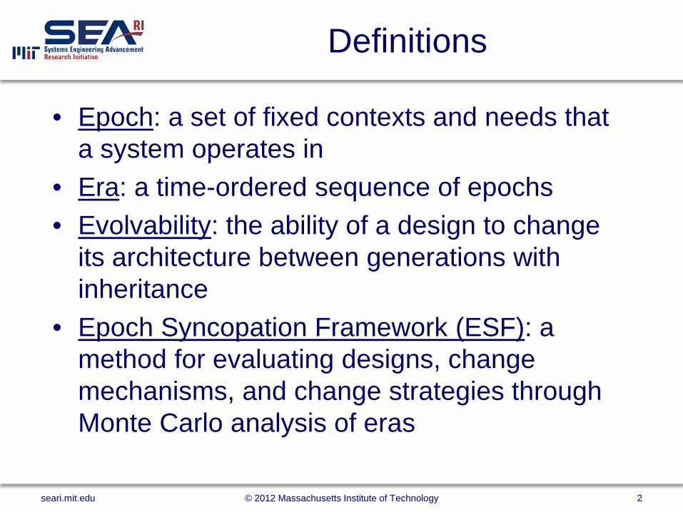
• 2 variables: mission (preference set) and technology level • Technology is either “present” or “future”
– Mean time between shifts: 8 years – Can only transition from present to future
• 8 Missions: (1) baseline, (2) technology demonstration, (3) GEO rescue, (4) deployment assistance, (5) refueling and maintenance, (6) garbage collector, (7) all-purpose military, and (8) satellite saboteur – Average mission duration: 4 years – Treated as contracts
seari.mit.edu 8 © 2012 Massachusetts Institute of Technology
Technology To Present To Future
From Present 0 1
From Future 0 1
Mission To 1 To 2 To 3 To 4 To 5 To 6 To 7 To 8 From 1 0.300 0.400 0.050 0.050 0.050 0.050 0.050 0.050 From 2 0.050 0.150 0.133 0.133 0.133 0.133 0.133 0.133 From 3 0.150 0.050 0.500 0.060 0.060 0.060 0.060 0.060 From 4 0.150 0.050 0.060 0.500 0.060 0.060 0.060 0.060 From 5 0.150 0.050 0.060 0.060 0.500 0.060 0.060 0.060 From 6 0.150 0.050 0.060 0.060 0.060 0.500 0.060 0.060 From 7 0.150 0.050 0.038 0.038 0.038 0.038 0.500 0.150 From 8 0.150 0.050 0.038 0.038 0.038 0.038 0.150 0.500
Space Tug Epoch Variables
• 2 variables: mission (preference set) and technology level • Technology is either “present” or “future”
– Mean time between shifts: 8 years – Can only transition from present to future
• 8 Missions: (1) baseline, (2) technology demonstration, (3) GEO rescue, (4) deployment assistance, (5) refueling and maintenance, (6) garbage collector, (7) all-purpose military, and (8) satellite saboteur – Average mission duration: 4 years – Treated as contracts
seari.mit.edu 9 © 2012 Massachusetts Institute of Technology
Technology To Present To Future
From Present 0 1
From Future 0 1
Mission To 1 To 2 To 3 To 4 To 5 To 6 To 7 To 8 From 1 0.300 0.400 0.050 0.050 0.050 0.050 0.050 0.050 From 2 0.050 0.150 0.133 0.133 0.133 0.133 0.133 0.133 From 3 0.150 0.050 0.500 0.060 0.060 0.060 0.060 0.060 From 4 0.150 0.050 0.060 0.500 0.060 0.060 0.060 0.060 From 5 0.150 0.050 0.060 0.060 0.500 0.060 0.060 0.060 From 6 0.150 0.050 0.060 0.060 0.060 0.500 0.060 0.060 From 7 0.150 0.050 0.038 0.038 0.038 0.038 0.500 0.150 From 8 0.150 0.050 0.038 0.038 0.038 0.038 0.150 0.500
These transition matrices and duration parameters will be used to construct the eras

Space Tug Design Set3
• 4 Design Variables • “DfE” represents
inclusion of evolvability design principles (modularity, margin, etc.) with cost/schedule penalties
• Propulsion type and DfE determine architecture for this simulation • Schedule calculated based on architecture
• Where 2 values are given: (Present Tech/Future Tech) • 2 month penalty added to initial schedule if DfE included
seari.mit.edu 10 © 2012 Massachusetts Institute of Technology
3. McManus, H. and Schuman, T. “Understanding the Orbital Transfer Vehicle Trade Space,” proceedings of AIAA Space 2003, Long Beach, CA, Sept. 2003.
Design Variables Levels
Manipulator Mass (kg) [300, 1000, 3000, 5000] Propulsion System Storable BiPropellant, Cryogenic, Electric, Nuclear Fuel Mass (kg) [30, 100, 300, 600, 1200, 3000, 10000, 30000] DfE (% Mass Penalty) [0, 20]
Propulsion System Isp (sec) Base Mass (kg) Mass Fract. Fast? Baseline Schedule (months) Storable BiProp 300 0 0.12 Y 8 Cryo 450/550 0 0.13 Y 9 Electric 3000 25 0.25/.3 N 10 Nuclear 1500 1000/600 0.20 Y 12

DfE Transitions
• Single transition mechanism: “redesign with inheritance” • If current design does not include DfE, redesign cost is just the
cost of the new design • If current design includes DfE, mass of continuing components
reduced by “reuse advantage” – Mass maps to cost in space tug – Redesign advantage = 50% in this simulation
• Redesign schedule is the same as initial schedule if DfE is not included in current design
• If current design has DfE, initial schedule is reduced by evolvability advantage to get redesign schedule – Evolvability advantage = 3 months – No penalty or advantage for discontinuing DfE
seari.mit.edu 11 © 2012 Massachusetts Institute of Technology
“Redesign with inheritance” is used to illustrate the way a transition rule would be implemented, not a proposed model
Example Data
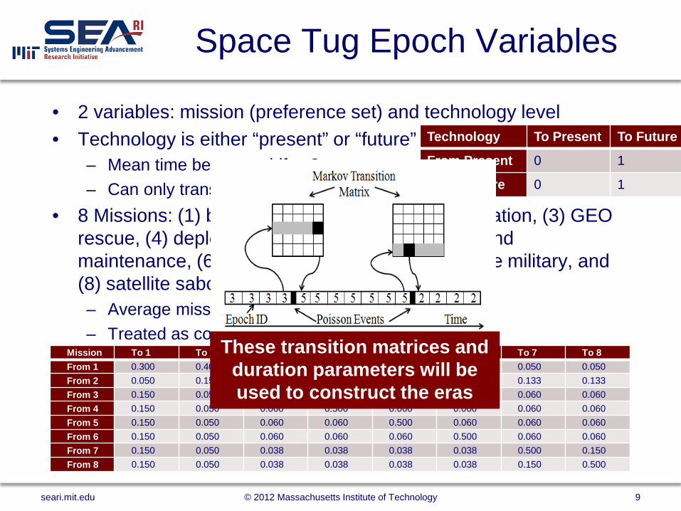
• Gave the same era and starting design to each strategy – Chart below shows the initial epoch and 4 subsequent epoch shifts
• Starting design was 155 – 300 kg manipulator,
electric propulsion, 300 kg fuel, includes DfE
• 40th percentile used for strategies 2 and 3 • 4 year generation length used for strategy 3 • Aggregate data shown here: • Strategy 1 has better
performance, but at 4 times the cost
seari.mit.edu 12 © 2012 Massachusetts Institute of Technology
Month 1 12 78 96 102
Mission 1 3 3 8 4
Tech Present Present Future Future Future
Epoch ID 1 3 11 16 12
Strategy LC_Cost ($M) Time Below (Months) TWAU
Strat 1 2,030 21 0.8833
Strat 2 (40) 549 22 0.6195
Strat 3 (40/4 yrs) 549 57 0.4157
These results capture overall performance, but give us little information about what happened during the era.

Example Trajectories
seari.mit.edu 13 © 2012 Massachusetts Institute of Technology
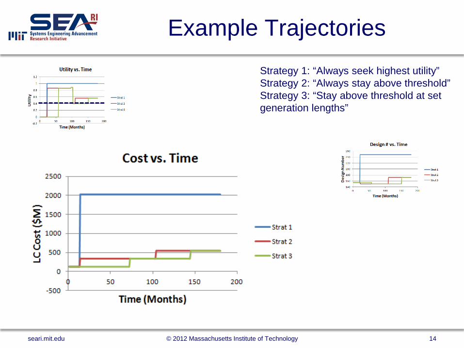
Strategy 1: “Always seek highest utility” Strategy 2: “Always stay above threshold” Strategy 3: “Stay above threshold at set generation lengths”
Example Trajectories
seari.mit.edu 14 © 2012 Massachusetts Institute of Technology
Strategy 1: “Always seek highest utility” Strategy 2: “Always stay above threshold” Strategy 3: “Stay above threshold at set generation lengths”
Example Trajectories
seari.mit.edu 15 © 2012 Massachusetts Institute of Technology
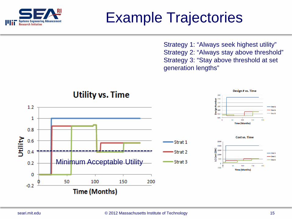
Strategy 1: “Always seek highest utility” Strategy 2: “Always stay above threshold” Strategy 3: “Stay above threshold at set generation lengths”
Minimum Acceptable Utility

Example Data Discussion
• When Design 155 was fielded in month 13, the mission had just changed from 1 to 3 (month 12) – Mission 1 Utility (Design 155) = 0.65 – Mission 3 Utility (Design 155) = 0 (slow mover) – Redesign immediately initiated in strategies 1 and 2
• Strategy 3 trajectories reached same values as strategy 2 trajectories, but lagged – Same logic applied at different
points in era • Here strategy 3 was dominated
by strategy 2 in all categories – Not always the case, especially
with volatile eras
seari.mit.edu 16 © 2012 Massachusetts Institute of Technology
Mission Shift
Design Fielded
Setting up Simulation
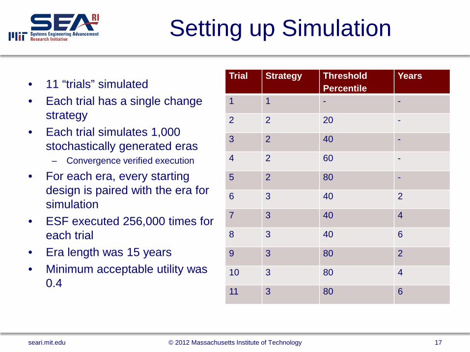
• 11 “trials” simulated • Each trial has a single change
strategy • Each trial simulates 1,000
stochastically generated eras – Convergence verified execution
• For each era, every starting design is paired with the era for simulation
• ESF executed 256,000 times for each trial
• Era length was 15 years • Minimum acceptable utility was
0.4
seari.mit.edu 17 © 2012 Massachusetts Institute of Technology
Trial Strategy Threshold Percentile
Years
1 1 - -
2 2 20 -
3 2 40 -
4 2 60 -
5 2 80 -
6 3 40 2
7 3 40 4
8 3 40 6
9 3 80 2
10 3 80 4
11 3 80 6
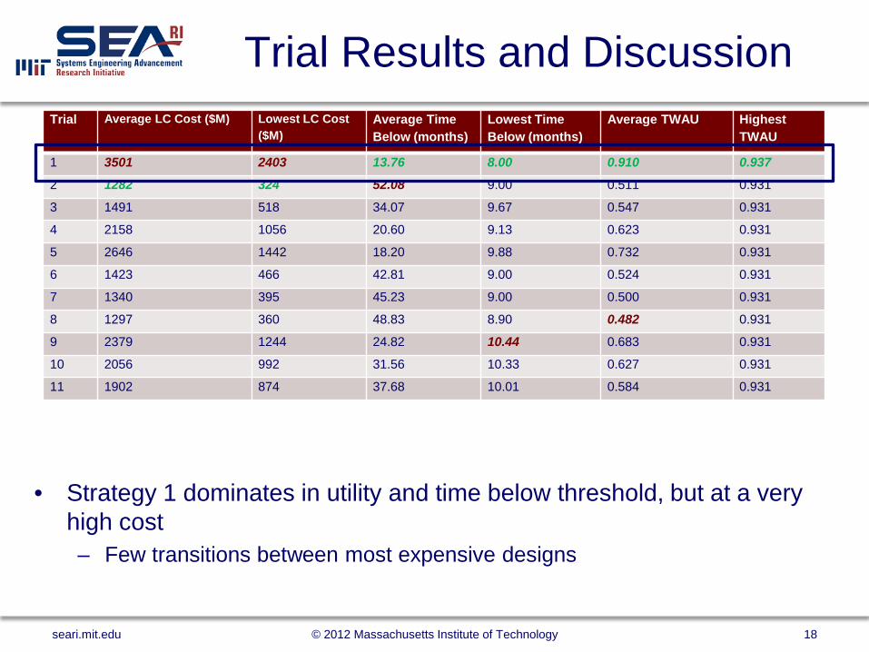
Trial Results and Discussion Trial Average LC Cost ($M) Lowest LC Cost
($M) Average Time Below (months)
Lowest Time Below (months)
Average TWAU Highest TWAU
1 3501 2403 13.76 8.00 0.910 0.937
2 1282 324 52.08 9.00 0.511 0.931
3 1491 518 34.07 9.67 0.547 0.931
4 2158 1056 20.60 9.13 0.623 0.931
5 2646 1442 18.20 9.88 0.732 0.931
6 1423 466 42.81 9.00 0.524 0.931
7 1340 395 45.23 9.00 0.500 0.931
8 1297 360 48.83 8.90 0.482 0.931
9 2379 1244 24.82 10.44 0.683 0.931
10 2056 992 31.56 10.33 0.627 0.931
11 1902 874 37.68 10.01 0.584 0.931
seari.mit.edu 18 © 2012 Massachusetts Institute of Technology
• Strategy 1 dominates in utility and time below threshold, but at a very high cost – Few transitions between most expensive designs

Trial Results and Discussion Trial Average LC Cost ($M) Lowest LC Cost
($M) Average Time Below (months)
Lowest Time Below (months)
Average TWAU Highest TWAU
1 3501 2403 13.76 8.00 0.910 0.937
2 1282 324 52.08 9.00 0.511 0.931
3 1491 518 34.07 9.67 0.547 0.931
4 2158 1056 20.60 9.13 0.623 0.931
5 2646 1442 18.20 9.88 0.732 0.931
6 1423 466 42.81 9.00 0.524 0.931
7 1340 395 45.23 9.00 0.500 0.931
8 1297 360 48.83 8.90 0.482 0.931
9 2379 1244 24.82 10.44 0.683 0.931
10 2056 992 31.56 10.33 0.627 0.931
11 1902 874 37.68 10.01 0.584 0.931
seari.mit.edu 19 © 2012 Massachusetts Institute of Technology
20 40 60 80 40 40 40 80 80 80
• As utility threshold increases for strategies 2 and 3 – LC cost increases, time below acceptability decreases, utility increases
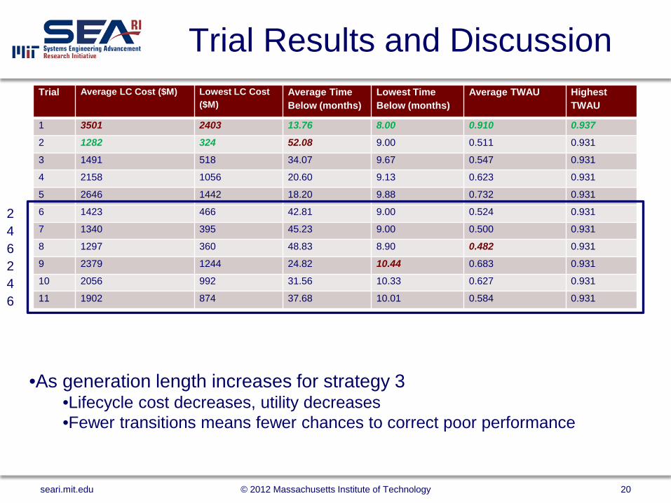
Trial Results and Discussion Trial Average LC Cost ($M) Lowest LC Cost
($M) Average Time Below (months)
Lowest Time Below (months)
Average TWAU Highest TWAU
1 3501 2403 13.76 8.00 0.910 0.937
2 1282 324 52.08 9.00 0.511 0.931
3 1491 518 34.07 9.67 0.547 0.931
4 2158 1056 20.60 9.13 0.623 0.931
5 2646 1442 18.20 9.88 0.732 0.931
6 1423 466 42.81 9.00 0.524 0.931
7 1340 395 45.23 9.00 0.500 0.931
8 1297 360 48.83 8.90 0.482 0.931
9 2379 1244 24.82 10.44 0.683 0.931
10 2056 992 31.56 10.33 0.627 0.931
11 1902 874 37.68 10.01 0.584 0.931
seari.mit.edu 20 © 2012 Massachusetts Institute of Technology
•As generation length increases for strategy 3 •Lifecycle cost decreases, utility decreases •Fewer transitions means fewer chances to correct poor performance
2 4 6 2 4 6
Discussion Cont’d
• The best performing designs with respect to lifecycle cost showed the following: – 300 kg manipulator mass, Nuclear or Electric propulsion – 30-300 kg of fuel, included DfE – Did not include expensive, potentially unnecessary options
• The best performing designs with respect to time below acceptability and TWAU showed the following: – 3,000-5,000 kg manipulator mass, any propulsion other than electric – 30,000 kg of fuel, no DfE included – Expensive, but high performance in most epochs
• DfE not needed since they rarely needed to transition
seari.mit.edu 21 © 2012 Massachusetts Institute of Technology

Space Tug Conclusions
• Space tug case study – For minimizing lifecycle cost, strategy 3 was best overall,
particularly with low utility thresholds and longer generations – Strategy 1 was best for minimizing time below acceptability
and maximizing utility
• Are the utility and time benefits worth the extra cost?
seari.mit.edu 22 © 2012 Massachusetts Institute of Technology
0.4
0.5
0.6
0.7
0.8
0.9
1
1000 1500 2000 2500 3000 3500 4000
Aver
age
TWAU
Average Lifecycle Cost ($M)
TWAU vs LC Cost
Strategy 1
Strategy 2
Strategy 3
0
10
20
30
40
50
60
1000 1500 2000 2500 3000 3500 4000
Aver
age
Tim
e Be
low
(Mon
ths)
Average Lifecycle Cost ($M)
Time Below vs LC Cost
Strategy 1
Strategy 2
Strategy 3

Conclusions
• ESF provides insights not seen in other methods – The sequencing of
epochs impacts performance
– The timing impacts of executing a change mechanism impact performance
seari.mit.edu 23 © 2012 Massachusetts Institute of Technology
ESF Future Work • Refine era constructor
stochastic modeling – Have transition matrix
become a function of time between shifts for certain types of epoch variables
• Develop more change strategies
• Apply to more data sets – More system examples – SoS applications
QUESTIONS?
seari.mit.edu 24 © 2012 Massachusetts Institute of Technology