EVALUATING SAMPLING STRATEGIES FOR RAINFALL …

University of Kentucky University of Kentucky

UKnowledge UKnowledge

Theses and Dissertations--Biosystems and Agricultural Engineering Biosystems and Agricultural Engineering

2014

EVALUATING SAMPLING STRATEGIES FOR RAINFALL EVALUATING SAMPLING STRATEGIES FOR RAINFALL

SIMULATION STUDIES AND SURFACE TRANSPORT OF SIMULATION STUDIES AND SURFACE TRANSPORT OF

ANTIBIOTICS FROM SWINE MANURE APPLIED TO FESCUE ANTIBIOTICS FROM SWINE MANURE APPLIED TO FESCUE

PLOTS PLOTS

Holly K. Enlow University of Kentucky, [email protected]

Right click to open a feedback form in a new tab to let us know how this document benefits you. Right click to open a feedback form in a new tab to let us know how this document benefits you.

Recommended Citation Recommended Citation Enlow, Holly K., "EVALUATING SAMPLING STRATEGIES FOR RAINFALL SIMULATION STUDIES AND SURFACE TRANSPORT OF ANTIBIOTICS FROM SWINE MANURE APPLIED TO FESCUE PLOTS" (2014). Theses and Dissertations--Biosystems and Agricultural Engineering. 21. https://uknowledge.uky.edu/bae_etds/21

This Master's Thesis is brought to you for free and open access by the Biosystems and Agricultural Engineering at UKnowledge. It has been accepted for inclusion in Theses and Dissertations--Biosystems and Agricultural Engineering by an authorized administrator of UKnowledge. For more information, please contact [email protected].

http://uknowledge.uky.edu/

http://uknowledge.uky.edu/

https://uknowledge.uky.edu/

https://uknowledge.uky.edu/bae_etds

https://uknowledge.uky.edu/bae_etds

https://uknowledge.uky.edu/bae

https://uky.az1.qualtrics.com/jfe/form/SV_9mq8fx2GnONRfz7

mailto:[email protected]

STUDENT AGREEMENT: STUDENT AGREEMENT:

I represent that my thesis or dissertation and abstract are my original work. Proper attribution

has been given to all outside sources. I understand that I am solely responsible for obtaining

any needed copyright permissions. I have obtained needed written permission statement(s)

from the owner(s) of each third-party copyrighted matter to be included in my work, allowing

electronic distribution (if such use is not permitted by the fair use doctrine) which will be

submitted to UKnowledge as Additional File.

I hereby grant to The University of Kentucky and its agents the irrevocable, non-exclusive, and

royalty-free license to archive and make accessible my work in whole or in part in all forms of

media, now or hereafter known. I agree that the document mentioned above may be made

available immediately for worldwide access unless an embargo applies.

I retain all other ownership rights to the copyright of my work. I also retain the right to use in

future works (such as articles or books) all or part of my work. I understand that I am free to

register the copyright to my work.

REVIEW, APPROVAL AND ACCEPTANCE REVIEW, APPROVAL AND ACCEPTANCE

The document mentioned above has been reviewed and accepted by the student’s advisor, on

behalf of the advisory committee, and by the Director of Graduate Studies (DGS), on behalf of

the program; we verify that this is the final, approved version of the student’s thesis including all

changes required by the advisory committee. The undersigned agree to abide by the statements

above.

Holly K. Enlow, Student

Dr. Carmen Agouridis, Major Professor

Dr. Donald Colliver, Director of Graduate Studies

EVALUATING SAMPLING STRATEGIES FOR RAINFALL SIMULATION

STUDIES AND SURFACE TRANSPORT OF ANTIBIOTICS FROM SWINE

MANURE APPLIED TO FESCUE PLOTS

____________________________________

THESIS

_____________________________________

A thesis submitted in partial fulfillment of the

requirements for the degree of Master of Science in Biosystems and Agricultural

Engineering in the College of Engineering at the University of Kentucky

By

Holly K. Enlow

Lexington, Kentucky

Director: Dr. Carmen T. Agouridis, Assistant Professor of

Biosystems and Agricultural Engineering

Lexington, Kentucky

2014

Copyright © Holly Kristina Enlow 2014

ABSTRACT OF THESIS




Antibiotics are commonly used in animal agriculture to treat and prevent diseases

and promote growth. Unfortunately, large amounts of antibiotics are not metabolized,

but instead are excreted in urine and feces. Rainfall simulation studies were used to

investigate the transport of the antibiotic oxytetracycline and various constituents in

runoff and the ability of alum to reduce pollutant transport. Runoff samples were

collected at several points during the simulated storm event from each of four treatments:

control (C), manure only (M), manure and antibiotics (MA), and manure, antibiotics and

alum (MAA). Flow-weighted composite samples were created and compared to the flow

weighted mean concentration (FWMC). Constituents with concentrations well-above the

detection limits (E. coli, NH4-N, turbidity, TSS, TOC, and EC) showed a strong

correlation between flow-weighted composite samples and FWMC. When constituent

concentrations were at or near the detection limits, errors associated with the composite

samples were magnified. Oxytetracycline concentrations had the strong correlation to E.

coli, Cl, TOC, TSS, and turbidity suggesting that a BMP effective at trapping sediment or

particulates may work best for reducing oxytetracycline concentrations in runoff. Alum

(1%) did not reduce levels of oxytetracycline in runoff. It is recommended that higher

doses of alum be tested.

KEYWORDS: Antibiotic, transport, runoff, alum, sampling

Holly Kristina Enlow

Signature

January 6, 2014

Date




By

Holly Kristina Enlow

Director of Thesis

Director of Graduate Studies

Date

Donald G. Colliver

January 6, 2014

Carmen T. Agouridis

For my grandparents

iii

ACKNOWLEDGEMENTS

This research was very much a team effort and would not have been possible without

the help and encouragement of many wonderful individuals. My graduate school

experience was greatly enhanced by all of the wonderful people in the Biosystems and

Agricultural Engineering Department. Without the advice, expertise, and assistance of

Alex Fogle and Lloyd Dunn, this project would not have been possible. Thank you for

your willingness to help me at every stage of this project, especially with the field work,

for fixing all of the things I broke along the way, and for teaching me the importance of

making work fun. To Dr. Manish Kulshrestha, thank you for the countless hours spent in

the lab, your persistence in solving all of the issues that arose throughout antibiotic

analysis process, and for ensuring me that we would figure it out eventually. I would like

to thank my fellow graduate students for all of your encouragement and support

throughout my graduate education. It was joy spending time with you and getting to

know all of you. A special thanks goes to the “X-Stream Team”, Whitney Blackburn-

Lynch, John McMaine, Mary Weatherford, Mariana da Rosa, and Zach Tyler, for your

willingness to assist with my research, even if it was not the most glamorous of jobs.

I am extremely thankful for the love and support of my family and friends. To my

Mom thank you for your encouragement and support throughout all of my academic

efforts and for giving me a desire to learn. To my Dad, thank you for instilling in me a

love for agriculture and teaching me about conservation and the environment at a very

young age. To my sister, thank you for setting such a great example and inspiring me to

pursue my master’s degree.

iv

I would like to thank my committee members, Dr. Dwayne Edwards and Dr.

Lindell Ormsbee, for their advice and suggestions throughout the course of my research.

Finally, I would like to express my deep gratitude to my advisor Dr. Carmen Agouridis

for all of her help, encouragement, and mentorship she has given throughout this whole

process and for always having an open door when I needed to talk. I would especially

like to thank her for her time and patience during the reviewing and editing stages.

v

TABLE OF CONTENTS

ACKNOWLEDGEMENTS ........................................................................................... III

LIST OF TABLES ....................................................................................................... VIII

LIST OF FIGURES ........................................................................................................ IX

CHAPTER 1: INTRODUCTION .................................................................................... 1

1.1 INTRODUCTION..................................................................................................... 1

1.2 OBJECTIVES ........................................................................................................... 9

1.3 ORGANIZATION OF THESIS ................................................................................ 9

CHAPTER 2: COMPARISON OF WATER QUALITY SAMPLING

TECHNIQUES FOR RAINFALL SIMULATION STUDIES ................................... 10

2.1 INTRODUCTION................................................................................................... 10

2.2 MATERIALS AND METHODS ............................................................................ 12

2.2.1 Study Site .......................................................................................................... 12

2.2.2 Plot Selection ................................................................................................... 13

2.2.3 Treatments........................................................................................................ 13

2.2.4 Rainfall ............................................................................................................. 15

2.2.5 Runoff Sample Collection ................................................................................ 15

2.2.6 Laboratory Analysis ......................................................................................... 16

2.2.6.1 Antibiotic Analysis ............................................................................................... 16

2.2.7 Data Analysis ................................................................................................... 17

2.3 RESULTS AND DISCUSSION .............................................................................. 17

2.4 CONCLUSIONS .......................................................................................................... 31

CHAPTER 3: RELATIONSHIPS BETWEEN OXYTETRACYCLINE AND

OTHER WATER QUALITY CONSTITUENTS ........................................................ 33

3.1 INTRODUCTION................................................................................................... 33


3.2.1 Study Site .......................................................................................................... 36

3.2.2 Plot Selection ................................................................................................... 36

vi

3.2.3 Experimental Treatments ................................................................................. 37

3.2.4 Rainfall ............................................................................................................. 38




3.2.7 Data Analysis ................................................................................................... 41

3.3 RESULTS AND DISCUSSION .............................................................................. 41

3.3.1 Manure and Soil Sampling............................................................................... 41

3.3.2 Antibiotic Losses via Runoff............................................................................. 42

3.3.3 Oxytetracycline and Constituent Correlations ................................................ 47

3.3.4. Best Management Practice Selection .............................................................. 53

3.4 CONCLUSIONS ..................................................................................................... 58

CHAPTER 4: EFFECT OF ALUM ON SURFACE TRANSPORT OF

OXYTETRACYCLINE ................................................................................................. 59

4.1 INTRODUCTION................................................................................................... 59


4.2.1 Study Site .......................................................................................................... 61

4.2.2 Plot Selection ................................................................................................... 61

4.2.3 Experimental Treatments ................................................................................. 62

4.2.4 Rainfall ............................................................................................................. 63




4.2.7 Data Analysis ................................................................................................... 65

4.3 RESULTS AND DISCUSSION ....................................................................................... 65

4.3.1 Treatment Effects ............................................................................................. 65

4.3.1.1 Non-significant Constituents ................................................................................ 66

4.3.1.2 Significant Constituents ........................................................................................ 68

4.3.2 Time Effects ...................................................................................................... 79

4.4 CONCLUSIONS ..................................................................................................... 82

vii

CHAPTER 5: SUMMARY OF CONCLUSIONS ....................................................... 84

CHAPTER 6: FUTURE WORK ................................................................................... 86

APPENDIX A: RAINFALL SIMULATOR CALIBRATION AND PLOT CURVE

NUMBER DETERMINATION ..................................................................................... 87

A.1.1 RAINFALL SIMULATOR CALIBRATION ................................................................... 88

A.1.2 PLOT CURVE NUMBER DETERMINATION .............................................................. 92

APPENDIX B: FLOW-WEIGHTED COMPOSITE SAMPLE DATA .................... 96

APPENDIX C: METHODOLOGY FOR E.COLI ANALYSIS ................................ 113

C.1 BUFFER WATER AND DI WATER PREPARATION ...................................................... 114

C.1.1 Prepare Solutions .......................................................................................... 114

C.1.2 Prepare Buffer Water .................................................................................... 114

C1.3 Prepare DI H2O ............................................................................................. 114

C.1.4 Autoclave ....................................................................................................... 114

C.2 DILUTION BOTTLE PREPARATION ........................................................................... 115

C.3 DILUTIONS ............................................................................................................. 115

APPENDIX D: METHODOLOGY FOR ANTIBIOTIC EXTRACTION AND

ANALYSIS .................................................................................................................... 118

D.1 SAMPLE PREPARATION .......................................................................................... 119

D.2 LYOPHILIZATION ................................................................................................... 119

D.3 SAMPLE CONCENTRATION ..................................................................................... 119

D.4 HPLC .................................................................................................................... 120

APPENDIX E: MANURE AND SOIL SAMPLING RESULTS .............................. 121

REFERENCES .............................................................................................................. 124

VITA............................................................................................................................... 135

viii

LIST OF TABLES

Table 1.1. Top Producing States for Each Category of Livestock and Total Production. .. 3

Table 1.2. Excretion Rates of Commonly used Veterinary Antibiotics. ............................ 6

Table 2.1. Curve Numbers (CN) of Plots Used in the Study. ........................................... 13

Table 2.2. Assignment of Treatments to Plots. ................................................................. 14

Table 2.3. Results of Regressing FWMC vs. Flow-Weighted Composite Concentration.18

Table 3.1. Curve Numbers of Plots Used in the Study. .................................................... 37

Table 3.2. Treatment Associated with Each Plot. ............................................................. 37

Table 3.3. Manure Sampling Results. ............................................................................... 42

Table 3.4. Soil Sampling Results. ..................................................................................... 42

Table 3.5 Flow Normalized Oxytetracylcine Levels per Treatment................................. 42

Table 3.6. Oxytetracyline Losses (%) via Runoff from MA Plots. .................................. 47

Table 3.7. Pearson Correlation Coefficients (r) between Oxytetracycline Concentrations

and Constituent Concentrations for C and M Treatments.1 .............................................. 48

Table 4.1 Curve Numbers of Plots Used in the Study. ..................................................... 62

Table 4.2 Treatment Associate with Each Plot. ................................................................ 63

Table 4.3. Statistics for Runoff Variables (Mean ± Standard Deviation). ........................ 66

Table 4.4 Statistics for Constituent Concentrations at Time Intervals (Mean ± Standard

Deviation). ........................................................................................................................ 81

ix

LIST OF FIGURES

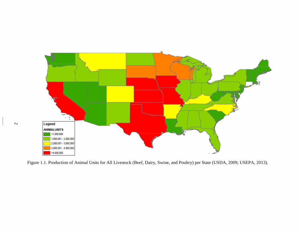
Figure 1.1. Production of animal units for all livestock (beef, dairy, swine, and poultry)

per state (USDA, 2009; USEPA, 2013). ............................................................................. 2

Figure 2.1. Comparison of FWMC and Flow-weighted Composite for ln E. coli. .......... 19

Figure 2.2. Comparison of FWMC and Flow-weighted Composite for ln NO3. .............. 20

Figure 2.3. Comparison of FWMC and Flow-weighted Composite for ln NH4. .............. 21

Figure 2.4. Comparison of FWMC and Flow-weighted Composite for ln PO4. .............. 22

Figure 2.5. Comparison of FWMC and Flow-weighted Composite for ln pH. ................ 23

Figure 2.6. Comparison of FWMC and Flow-weighted Composite for ln EC. ................ 24

Figure 2.7. Comparison of FWMC and Flow-weighted Composite for ln TSS. .............. 25

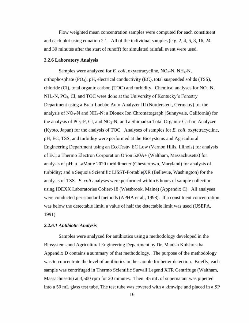
Figure 2.8. Comparison of FWMC and Flow-weighted Composite for ln TOC. ............. 26

Figure 2.9. Comparison of FWMC and Flow-weighted Composite for ln Turbidity. ...... 27

Figure 2.10. Comparison of FWMC and Flow-weighted Composite for ln

Oxytetracycline. ................................................................................................................ 28

Figure 2.11. Comparison of FWMC and Flow-weighted Composite for ln C1-. ............. 29

Figure 3.1. Oxytetracycline concentrations normalized by flow rate from a MA plot (B6).

........................................................................................................................................... 43

Figure 3.2. Oxytetracycline concentrations normalized by flow rate for a C plot (C2). .. 45

Figure 3.3. Oxytetracycline concentrations normalized by flow rate at M plot (B4). ...... 46

Figure 3.4. Relationship between Oxytetracycline and pH for the MA Plots. ................. 49

Figure 3.5. Relationship between Oxytetracycline and NO3-N for the MA Plots. ........... 50

Figure 3.6. Relationship between Oxytetracycline and PO4 for MA Plots. ..................... 51

Figure 3.7. E. coli Concentrations for M and MA Plots During the Simulated Storm ..... 52

Figure 3.8. Relationship between Oxytetracyline and Cl for MA Plots. .......................... 54

Figure 3.9. Relationship between Oxytetracycline and TOC for MA Plots. .................... 55

Figure 3.10. Relationship between Oxytetracycline and EC for MA Plots. ..................... 56

Figure 3.11. Relationship between Oxytetracycline and Turbidity MA Plots. ................. 57

Figure 4.1. Flow Normalized ln Cl Concentrations for Each Treatment. C=Control,

M=Manure Only, MA=Manure and Antibiotics, and MAA=Manure, Antibiotics and

Alum. ................................................................................................................................ 67

x

Figure 4.2. Flow Normalized ln TOC Concentrations for Each Treatment. C=Control,


Alum. ................................................................................................................................ 69

Figure 4.3. Flow Normalized ln pH Concentrations for Each Treatment. C=Control,


Alum. ................................................................................................................................ 70

Figure 4.4. Flow Normalized ln EC Concentrations for Each Treatment. C=Control,


Alum. ................................................................................................................................ 71

Figure 4.5. Flow Normalized ln TSS Concentrations for Each Treatment. C=Control,


Alum. ................................................................................................................................ 72

Figure 4.6. Flow Normalized ln Turbidity Concentrations for Each Treatment.

C=Control, M=Manure Only, MA=Manure and Antibiotics, and MAA=Manure,

Antibiotics and Alum. ....................................................................................................... 73

Figure 4.7. Flow Normalized ln E. coli Concentrations for Each Treatment. C=Control,


Alum. ................................................................................................................................ 74

Figure 4.8. Flow Normalized ln NO3-N Concentrations for Each Treatment. C=Control,


Alum. ................................................................................................................................ 76

Figure 4.9. Flow Normalized ln NH4-N Concentrations for Each Treatment. C=Control,


Alum. ................................................................................................................................ 77

Figure 4.10. Flow Normalized ln PO4-P Concentrations for Each Treatment. C=Control,


Alum. ................................................................................................................................ 78

Figure 4.11. Flow Normalized ln Oxytetracycline Concentrations for Each Treatment.


Antibiotics and Alum. ....................................................................................................... 80

1

CHAPTER 1: INTRODUCTION

1.1 INTRODUCTION

Animal agriculture generates over $154 billion in sales annually in the United

States (USDA, 2009). Though the number of livestock and poultry operations in the U.S.

has decreased by 80% since the 1950’s, production has more than doubled (USEPA,

2013). Livestock operations are now larger in size and are more geographically

concentrated in the central portion of the U.S. (Figure 1.1). Over half of swine facilities,

for example, are located within one mile of another animal agriculture operation (USDA,

2001). Table 1.1 contains top livestock producing states for each livestock category as

well as total livestock production. The greatest numbers of animal units (1 animal unit,

AU, equals 454 kg) are associated with beef cattle with Texas, Missouri and Oklahoma

producing a combined total of over 9.4 million AUs. Iowa, North Carolina, and

Minnesota are the top three swine producing states with nearly 4.8 million AUs.

California, Wisconsin, and New York are the leading dairy production states, and North

Carolina, Arkansas and Georgia are the leading poultry production states. Considering

beef, swine, dairy and poultry together, the largest livestock producing states are Texas,

Iowa, Nebraska, California, and Kansas; hence four of the top five states are located in

the central U.S.

The USEPA (2013) estimated that livestock and poultry operations in the U.S.

generate over 1.1 billion tons of manure on an annual basis. High concentrations of

livestock, as seen in Figure 1.1, means producers must manage large amounts of manure

oftentimes with insufficient amounts of cropland on which to apply this manure. Ideally,

agricultural operations would utilize integrated crops and livestock production methods

whereby animal manure serves as a fertilizer for nearby croplands. But because these

more concentrated livestock operations generate large quantities of manure, and nutrients

in greater volumes than those required by crops, developing a sound and sustainable

manure management plan with limited land resources is quite challenging. This is

especially true as nutrient management systems shift towards basing manure application

rates on phosphorus levels rather than nitrogen levels (Higgins et al., 2013). As noted by

Eghball and Power (1999), crops require less phosphorus as compared to nitrogen; hence

2

Figure 1.1. Production of Animal Units for All Livestock (Beef, Dairy, Swine, and Poultry) per State (USDA, 2009; USEPA, 2013).

3

Table 1.1. Top Producing States for Each Category of Livestock and Total Production.

State Rank

Beef Swine Dairy Poultry Total Livestock

State Total AU1 State Total AU State Total AU State Total AU State Total AU

1 TX 5,259 IA 2,409 CA 2,487 NC 647 TX 11,109

2 MO 2,089 NC 1,382 WI 1,688 AR 642 IA 5,587

3 OK 2,063 MN 999 NY 847 GA 594 NE 5,236

4 NE 1,889 IL 607 PA 748 AL 431 CA 5,235

5 SD 1,649 IN 486 ID 725 TX 367 KS 4,933

6 MT 1,522 NE 462 MN 621 MS 356 OK 4,571

7 KS 1,516 MO 435 TX 546 MN 335 MO 4,179

8 TN 1,179 OK 367 MI 465 CA 282 MN 3,269

9 KY 1,166 KS 256 NM 441 IA 279 WI 3,213

10 AR 947 OH 243 OH 367 MO 260 SD 3,180

11 FL 942 SD 207 WA 329 VA 203 NC 2,704

12 ND 930 PA 160 IA 291 SC 201 CO 2,183

13 IA 904 TX 152 AZ 248 PA 201 MT 2,172

14 CO 735 MI 141 IN 225 IN 198 AR 2,164

15 WY 732 CO 141 VT 189 OH 161 KY 2,143 Source: (USDA, 2009) 1AU= 1 animal unit=454 kg of live weight or one beef cattle. Numbers are in 1000’s of AUs.

4

lesser amount of manure should be applied to the land to help prevent water quality

impairment.

Presently, manure management systems for large livestock operations are

designed to store manure in lagoons or pit systems before periodic land application. And

while contaminants can enter surface and ground waters through spills and leaks from

these storage systems, land application of manure is the primary pathway in which

pollutants enter our nation’s streams, rivers, lakes and estuaries. Ideally, operators base

manure application rates on crop requirements of nitrogen and/or phosphorus (USEPA

2013, NRCS 2012); however, this is not always the case. Nutrients, pathogens and other

such constituents not captured in croplands either through plant uptake, soil sorption, or

the like are transported via runoff to surface waters or infiltrated into shallow ground

waters (NSTC-CENR 2000; Campagnolo et al., 2002). Alexander et al. (2008)

concluded that agricultural sources, largely manure, contributed 70% of the nitrogen and

80% of the phosphorus found in the Gulf of Mexico. The authors noted that these

nutrients, of which Kentucky is a significant contributor, were largely transported to the

Gulf of Mexico via small and midsized streams. Currently, Kentucky currently ranks 15th

in the nation in total livestock production and 13th

in manure production (USDA, 2009).

Additionally, Kentucky has over 148,000 km of stream, many of which are first- or

second-order systems (KDOW, 2010).

While much research has been conducted on the environmental impacts of animal

agriculture as it relates to nutrients (Moore and Miller, 1994; Edwards et al., 2000; Smith

et al., 2001; Penn and Bryant, 2006; Alexander et al., 2008; USEPA, 2013) and

pathogens (Khaleel et al., 1980; Mawdsley et al., 1995; Gerba and Smith, 2005;

USEPA, 2013), far fewer studies have examined other contaminants such as hormones

and antibiotics (Kay et al., 2005; Chee-Sanford et al., 2009; LaShore and Pruden, 2009;

Kim et al., 2010; DeLuane and Moore, 2013). Antibiotic use is widespread in animal

agriculture as a means of combating diseases and infections in order help ensure the meat

supply is safe for human consumption. Unfortunately, it has become more common for

livestock operations to use antibiotics as a preventative tool against illness and as a

growth additive, particularly in large concentrated animal feeding operations or CAFOs

where living conditions are crowded (LaShore and Pruden, 2009). Oftentimes, feed is

5

supplemented with antibiotics to limit nutrient absorption by gastrointestinal microbes

thus ensuring more nutrients are available for absorption by the animal in order to

achieve more rapid weight gain (Kumar et al., 2005). Davis et al. (2006) estimated that

over 11 million kg of veterinary antibiotics were used for nontherapeutic uses in 2002

alone.

Large amounts of these administered antibiotics are not metabolized by livestock

but instead are excreted in manure. Tetracyclines, for example, which are one of the

most commonly used groups of antibiotics due to their broad spectrum applicability, are

excreted a rate of about 70 to 90 % (Kumar et al., 2005). Concentrations of antibiotics in

manure can range from 1-10 mg L-1

though concentrations as high as 200 mg L-1

have

been measured (Kumar et al., 2005). A typical daily dose of antibiotics for adult humans

ranges from 80 to 6,000 mg depending on the antibiotic and intended treatment (Hirsch et

al., 1999). Oxytetracyline is often administered at 1 to 2 g d-1

for a typical adult (NLM,

2005). The rate of excretion for other types of antibiotics (non-tetracyclines) ranges from

25-75% (Chee-Sanford et al., 2001). Table 1.2 contains excretion rates for commonly

used veterinary antibiotics. The large rate of excretion for tetracycline is of particular

concern because it is a widely used antibiotic, and land application of manure has been

attributed as the primary means by which veterinary antibiotics are introduced into the

terrestrial and subsequently aquatic environments (Baguer et al., 2000).

Because of these and other findings, the U.S. Environmental Protection Agency

(USEPA) classifies antibiotics as a contaminant of emerging concern (CEC) (USEPA,

2007). A CEC is one that is now being detected in the environment and/or is at higher

than expected levels, meaning it was not previously present in the environment or was

present at undetectable or very low levels (USEPA, 2007). The risk that CEC’s pose to

human health is often unknown as in the case of antibiotics. Surface and ground waters

are not routinely tested for antibiotics; therefore their impact on the health of humans, as

well as other biota, is largely unknown. Since antibiotics are designed to combat

bacteria, it is expected that the presence of antibiotics in the soil and water would have a

negative impact on microorganisms living in these environments (Kay et al., 2005). The

primary concern with the wide-spread release of antibiotics into the environment is the

development of strains of antibiotic-resistant bacteria. It is feared that the accumulation

6

Table 1.2. Excretion Rates of Commonly used Veterinary Antibiotics.

Antibiotic

Amount

Excreted in

Urine and

Feces (%)1

Animal1,2

Common Uses2

Tetracycline 80

Beef, dairy,

poultry, sheep,

swine, humans

Bacterial pneumonia, bacterial

enteritis, foot rot, jowl abscesses,

mastitis, growth Promotion

Chlortetracycline 75

Beef, dairy,

swine, poultry,

sheep



mastitis, growth promotion

Oxytetracycline 80

Beef, dairy,

poultry, sheep,

swine, fish,

humans



mastitis, growth promotion

Lincomycin 60 Swine, poultry,

humans

Bacterial enteritis, infectious

arthritis, dysentery, mycoplasmal

pneumonia, growth promotion

Tylosin 50-90 Beef, dairy,

swine, sheep

Foot rot, liver abscesses,

respiratory disease, infectious

arthritis, growth promotion

Erythromycin 50-90

Beef, dairy,

poultry, sheep,

swine, humans

Foot rot, liver abscesses,

respiratory disease, bacterial

enteritis, infectious arthritis,

growth promotion

Monensin 50-90 Beef, dairy Liver abscesses, coccidiosis,

growth promotion Source: Kumar (2005)

1 and USEPA (2013)

2

of antibiotics in human-consumed plants and animals may lead to the introduction of

antibiotic-resistant bacteria into the food and water supply hence threatening human

health (Kemper, 2007). Likewise, the presence of antibiotics such as penicillin, which is

the most commonly reported allergy inducing antibiotic (ACAAI, 2013), in the food and

water supply could result in potentially fatal allergic reactions (Kummerer, 2003).

Research into the transport of antibiotics to surface waters via runoff is limited.

Arikan et al. (2008) sampled streams in a predominately agricultural watershed and

analyzed the water samples for several different types of antibiotics. Chlortetracycline

and oxytetracycline were the most commonly identified antibiotics in the samples with

concentrations of 0.016 µg L-1

. The authors concluded that the antibiotics were

7

transported in runoff from nearby manure-amended fields, as no other potential sources

of antibiotics were identified. Dolliver and Gupta (2008a) collected runoff samples from

manure amended land over the course of three years. Peak antibiotic concentrations of

0.5, 57.5 and 6.0 µg L-1

were found for chlortetracycline, monesin, and tysolin,

respectively. Dolliver and Gupta (2008a) found the greatest period for antibiotic losses

occurred during the non-growing season after fall application of manure. In another

study, Dolliver and Gupta (2008b) measured peak concentrations of 210, 3175, and 2544

µg L-1

for chlortetracycline, monensin, and tysolin, respectively, in runoff from

unprotected manure stockpiles suggesting that manure storage is also a significant

contributor to the presence of antibiotics in the aquatic environment. Kay et al. (2005)

spiked liquid hog manure to levels of 18.9 mg L-1

for oxytetracycline and 25.6 mg L-1

for

sulphachloropyridazine and applied this mixture to runoff plots. Runoff samples were

analyzed for the two antibiotics with peak concentrations determined to be 32 µg L-1

for

oxytetracycline and 415.5 µg L-1

for sulphachloropyridazine, which corresponds to a

mass loss of 0.074% and 0.418%, respectively. This study concluded that overland flow

has the potential to transport veterinary antibiotics to surface waters. Davis et al. (2006)

applied seven antibiotics at concentrations of 1 mg L-1

to plots prior to rainfall

simulation. Tetracycline concentrations in runoff were determined to be 0.03 µg L-1

which corresponds to a 0.002% antibiotic loss. However, 65% of this loss was associated

with sediment suggesting that erosion control practices could help reduce antibiotic

transport. Studies have shown antibiotics at levels of 50 µg L-1

for tysolin and 34 µg L-1

for chlortetracycline can be toxic to some algal species (Halling-Sørensen, 2000). While

it is not known at what levels antibiotics have a significant impact on other aquatic life,

hormones have been shown to have adverse effects, such as defeminization or

demasculinization, on fish at levels as low as 10-120 ng L-1

(Durhan et al., 2006).

Only a few studies have examined methods to reduce the transport of runoff to

surface waters. Lin (2011) examined three veterinary antibiotics (sulfamethazine,

tysolin, and enrofloxacin) and found that vegetated buffer strips reduced antibiotic

transport by 40% for sulfamethazine and 75% for both tylosin and enrofloxacin

suggesting that vegetated buffer strips can provide reductions in antibiotic transport. It is

important to note that the degree of mobility differs between antibiotics. Sulfonamides,

8

such as sulfamethazine, are more mobile in an aqueous phase than antibiotics such as

tylosin and enrofloxacin which are more likely to bind to the soil. Tetracyclines also have

a stronger affinity for binding to the soil (Tolls, 2001). Other methods from wastewater

treatment engineering hold promise in reducing antibiotic transport. Stackelberg et al.

(2007) found that conventional water treatment methods such as clarification,

disinfection, and granular activated carbon filtration reduced the concentration of several

antimicrobials, including erythromycin, linconycine, sulfamethazine, sulfathiazole, and

sulfamethoxazole, in water from 0.1 µg L-1

to levels below detection. Aluminum sulfate

or alum, which is a flocculating agent commonly used in wastewater treatment to settle

out solids, is effective at reducing the transport of phosphorus, hormones, and some

metals (Edwards and Daniel, 1992; Moore and Miller, 1994; Moore et al., 1998; Edwards

et al., 1999; Smith et al., 2001; Penn and Bryant, 2006; DeLaune and Moore 2013).

Smith et al. (2001) used rainfall simulators to observe the surface transport of phosphorus

and noted an 84% reduction in phosphorus levels following the addition of alum to swine

manure. Alum has also been shown to reduce levels of hormones (17β-estradiol) in

runoff from plots amended with poultry litter by up to 40% (Delaune and Moore, 2013).

Tetracycline antibiotics bind strongly to manure particles suggesting that a process used

to flocculate manure particles might reduce the transport of tetracyclines as well. Based

on the results by Smith et al. (2001) and DeLaune and Moore (2013), it is possible that

alum, if used as a manure amendment, could reduce concentrations of antibiotics in

runoff.

Due to the uncontrollability and unpredictability of weather patterns, investigating

the transport of contaminants in overland flow is challenging. Hence, rainfall simulation

studies are often used (Miller, 1987; Bushee et al., 1998; Edwards et al., 1999; Edwards

et al., 2000; Smith et al., 2001; Sharpley and Kleinman, 2003; Davis et al., 2006; Kim et

al., 2010). One challenge with rainfall simulation studies is managing the large number

of samples generated as runoff samples are typically collected at several points during the

simulated storm event. To reduce analysis expenses and better manage sample analysis

time constraints, a single flow-weighted composite sample is created and analyzed in lieu

of analyzing each collected sample individually. It is thought that this single composite

sample will provide the same constituent values as analyzing multiple samples from a

9

single storm event and computing the flow-weighted mean concentration (FWMC),

which is a representation of a constituent’s concentration across the entire storm event

(Agouridis and Edwards, 2003) though the accuracy of this assumption for rainfall

simulation studies has not been tested.

1.2 OBJECTIVES

Research was conducted to examine the error associated with composite sampling

and to evaluate techniques antibiotic transport, specifically oxytetracycline, via runoff.

Rainfall simulators and fescue plots, located at the University of Kentucky’s Maine

Chance Research Farm, were used to achieve the following objectives:

1. Determine the error associated creating a single flow-weighted composite sample

as it relates to rainfall simulation studies.

2. Evaluate the relationship between oxytetracyline and E. coli, NO3-N, NH4-N,

PO4, pH, EC, TSS, Cl, TOC and turbidity levels.

3. Evaluate the effect of aluminum sulfate (alum) as a manure amendment on the

reduction of oxytetracycline levels in runoff.

1.3 ORGANIZATION OF THESIS

An overview of the research problem and objectives is described in Chapter 1.

Chapters 2-4 give detailed descriptions of the work done to accomplish the objectives of

this thesis. Chapter 5 discusses conclusions of the research, and Chapter 6 describes

potential future work.

10

CHAPTER 2: COMPARISON OF WATER QUALITY SAMPLING

TECHNIQUES FOR RAINFALL SIMULATION STUDIES

2.1 INTRODUCTION

Increases in discharge can affect water quality constituent concentrations

differently. While discharge can have an inverse relationship with dissolved pollutants

meaning higher discharge rates often result in lower concentrations via dilution, the

opposite is often seen with other pollutants such as suspended sediments and total metals

(Rickert, 1985). To account for this discharge-associated variation, the flow weighted

mean concentration (FWMC) is often used (Hoos et al., 2000; Agouridis and Edwards,

2003). The FWMC is defined as the total mass load of a constituent divided by the total

flow volume of an event (Huber, 1993; Cooke et al., 2000) and is presented in Agouridis

and Edwards (2003) as

∫ ( ) ( )

∫ ( ) ∑ (

)(

)

∑ (

)

(2.1)

In equation 2.1, the variable c represents concentration, Q represents flow, and t

represents time. As the FWMC is a single value that represents the concentration of a

constituent during a storm event (Agouridis and Edwards, 2003), it is important that this

value is computed using samples collected throughout the entire storm event to minimize

error (EPA, 1973; Mueller and Stone, 1998). Thus while the FWMC reduces a

constituent’s concentration for a storm event to a single value, it does not reduce the

number of samples one must analyze, and hence the costs one must incur.

Creating a composite sample is one method of reducing laboratory costs while

striving to maintain accuracy (i.e. minimizing error). With composite sampling, a single

sample is created by mixing defined portions of discrete samples (USEPA, 1982). These

defined portions are based on time (time compositing) or flow (flow-weighted

compositing). Discrete samples for time compositing are collected at uniform times, such

as every 20 minutes throughout the storm event, or at variable time increments

considering the first flush phenomenon. With variable time increments, samples are

collected at closer time increments at the start of the storm in an effort to capture the

11

rising limb and peak of the hydrograph as compared to later in the storm (Harmel and

King, 2005).

A number of studies have evaluated the accuracy of composite sampling

techniques when used to collect samples from streams. Aulenbach and Hooper (2005)

collected samples from mountain streams near Atlanta, Georgia using different sampling

scenarios, including weekly grab samples and flow-weighted and time-weighted samples,

for storm events. Alkalinity concentrations in the samples were used to predict the error

of a composite sampling strategy to determine stream loads. The study concluded

composite sampling produced a bias of ±0.8% which was within the error associated with

flow measurements and analytical chemistry. The study also noted that errors with time-

weighted and flow-weighted composite sampling were dependent on sampling design.

More frequent and a longer time interval for sampling produced more accurate results.

Even with some bias, flow-weighted composite sampling produced more accurate results

than the other sampling techniques, such as a time-weighted approach, which tended to

underestimate stream loads by 0.5% to 7.6%. Harmel et al. (2006) explored the

uncertainty in each stage of water quality data collection: streamflow measurement,

sample collection, sample storage, and laboratory analysis by compiling water quality

data on dissolved N and P, total N and P, and TSS, as well as streamflow measurements

from several other studies. When looking at the error for sampling strategies, this Harmel

et al. (2006) found an expected error for flow-weighted sampling of -6% to +17%

compared to an error associated with grab sampling of ±25% for dissolved constituents

and ±50% for sediment. Stone et al. (2000) also examined the differences between flow-

composited, time-composited, and grab sampling methods using the constituents nitrate

(NO3), ammonia (NH4), and total kjeldahl nitrogen (TKN). The authors concluded that

flow-weighting puts a greater emphasis on storm events rather than base flow conditions

in streams, which could result in an over-prediction of actual stream loadings due to the

more intensive monitoring that occurs during storm events. Stone et al. (2000) also noted

that if a grab sampling strategy is used, samples must be collected frequently, such as at

least twice a month, and at varying flow rates for data to be representative of actual

stream loadings.

12

While flow-weighted compositing may over-predict total stream loading, it is

better for characterizing runoff events. Harmel and King (2005) sampled sediment,

nitrate, and phosphate concentrations in twenty storm events in two small agricultural

watersheds in Texas. The authors determined that flow proportional sampling resulted in

an error of ±10% and represented storm loads better than time composited samples.

Harmel and King (2005) concluded that flow-weighted composite sampling was the

optimal way to balance data accuracy with limited resources.

Rainfall simulation studies are another means of investigation into contaminant

transport that is often used because of the ability to control rainfall amounts and patterns.

Rainfall simulators have been used to examine nutrient transport (Edwards et al. 1999;

Edwards et al., 2000; Smith et al.,2001; Sharpley and Kleinman, 2003), veterinary

pharmaceutical transport (Bushee et al., 1998; Davis et al., 2006; Kim et al., 2010), and

best management practice effectiveness (Edwards et al. 1999; Smith et al., 2001; Lin et

al., 2011). As with storm event sampling in streams, rainfall simulation studies generate

large numbers of samples as runoff is collected at several points during the simulated

storm event for multiple treatments and replications. To reduce analysis expenses and

better manage sample analysis time constraints, such as with Escherichia coli, oftentimes

a single flow-weighted composite sample is created and analyzed in lieu of analyzing

each collected sample individually and then computing the FWMC. It is hypothesized

that for rainfall simulation studies a single flow-weighted composite sample will provide

the same constituent values as the FWMC.

2.2 MATERIALS AND METHODS

2.2.1 Study Site

The study was performed at the rainfall simulation facility at the University of

Kentucky’s Maine Chance Research Farm (latitude: 38.1164°N; longitude: 84.4903W).

Edwards et al. (2000) thoroughly described the rainfall simulation facility, but briefly, the

facility consists of 75 plots with dimensions of 2.4 m by 6.1 m. Thirty of the plots are

individual while the remaining 45 are grouped linearly in six sets of five (Appendix A).

The five plots in each group can be hydrologically separated or combined to create a

longer flow path of 30.5 m. The plots have a 3% slope and are planted in Kentucky 31

13

fescue. The soil underlying the plots is a Maury silt loam (fine, mixed, mesic Typic

Paleudalf) (NRCS, 2013). Each plot is bordered with galvanized steel to ensure that

runoff does not leave the plot but is instead directed to a collection system located at the

most down-gradient end of the plot.

2.2.2 Plot Selection

In an attempt to minimize the variation associated with possible plot differences,

curve numbers (CN) were computed for 48 plots prior to the start of the study, as

described in Appendix A. Curve numbers were calculated for each of the thirty

individual plots as well as the uppermost and middle plots (sections) of the five plot sets.

Adjacent plots in the sets were not used to ensure rainfall from the simulators did not spill

over (i.e. edge effect). Based on these results, sixteen plots were identified for use in the

study (Table 2.1). Plots used in this study had a mean curve number of 83 ±4.

Table 2.1. Curve Numbers (CN) of Plots Used in the Study.

Plot CN Plot CN

B1 82 C5 89

B4 82 C6 77

B5 88 D1 86

B6 90 D5 84

B10 82 L1 84

C2 89 L3 79

C3 82 N2 77

C4 80 N9 81

2.2.3 Treatments

The treatments consisted of control (C), swine manure (M), swine manure plus an

antibiotic (MA), and swine manure plus an antibiotic and alum (MAA). The manure was

obtained from a hog facility in Bardstown, Kentucky. The facility did not administer

antibiotics to the hogs which were the source of the manure. The manure had a slurry

consistency, and it was stored in a pit prior to collection for this study. Collected manure

was stored in a 1,040 L polyethylene intermediate bulk container (IBC) tote at the

University of Kentucky Biosystems and Agricultural Engineering Department. For

14

mixing and transport to the study site, 55 L of manure was then transferred to a 208 L

plastic barrel. One plastic barrel was used for each treatment to prevent cross-

contamination.

For the MA and MAA treatments, the antibiotic oxytetracycline (300 mg mL-1

),

which was sold under the brand name Noromycin 300 LA (Norbrook, Lenexa, KS), was

added the manure in each respective barrel to produce a final concentration of 20 mg L-1

.

For the MAA treatment, liquid alum (Al2SO4, 48.5% solution) was added to the manure

in the respective barrel to produce a final concentration of 1.2 g L-1

(Bushee-Bullock,

1999). Uniform mixing was achieved using a custom mixer attached to a cordless drill.

The custom mixer, which was constructed in the Biosystems and Agricultural

Engineering Department, was approximately 1.5 m in length and had two 30 cm long fins

at a distance of 0 cm and 30 cm from the bottom. Once thoroughly mixed,the manure

mixtures (M, MA, or MAA) were applied to the respective plots at an application rate of

3 L m-2

, immediately prior to the start of simulated rainfall. This application rate

corresponded to 45L per plot. The target application rate was 112 kg N ha-1

as

recommended by AGR-1 (UK, 2012) and as done in Bushee-Bullock (1999). However,

based on laboratory results from the University of Kentucky Regulatory Services, the

actual application rate was about 150 kg N ha-1

. Treatments, which were part of a larger

study into antibiotic transport, were randomly assigned to the sixteen plots (Table 2.2).

Table 2.2. Assignment of Treatments to Plots.

Treatment1 Plots

C C2, C6, D12, D5

M B4, B83,C5, L1

MA B6, B10, C3, L3

MAA B1, B5, C4, N9 1 C=control; M =manure only; MA=manure plus antibiotics; MAA=manure plus antibiotics and alum

2D1 was not used in the E. coli analysis due to sampling error.

3B8 was not used in the analysis because it did not produce runoff

Three days prior to manure application, each plot was mowed resulting in a sward

height of 10 cm. Immediately prior to manure application, soil samples were collected

from each plot and manure samples were collected from the barrel for each treatment.

15

Soil samples were analyzed for P, K, Ca, Mg, Zn, pH, buffer pH, total nitrogen, and soil

texture at the University of Kentucky Regulatory Service laboratory while manure

samples were analyzed for N, P, K, Ca, Mg, Zn, Cu, Fe, and Mn.

2.2.4 Rainfall

Rainfall simulation began 30 minutes following manure application in order to

represent a worst-case scenario. Simulated rainfall was applied to the plots at a rate of

102 mm hr-1

and continued until 30 minutes following the start of runoff, after which

rainfall was stopped. Appendix A contains the calibration curves for the rainfall

simulators used in the study.

2.2.5 Runoff Sample Collection

Runoff samples were collected in 1 L autoclaved polyethylene bottles at intervals

of 2, 4, 6, 8, 16, 24 and 30 minutes after the start of runoff. A stopwatch was used to

record the time required to fill the sample bottle at each time interval. Using the time (t)

required to fill a sample bottle along with the volume (V) of each sample, flow rates (Q)

for each time interval were computed.

Composite samples were made by placing a defined volume of sample (SV) from

each time interval into a single bottle. The SV for each of the seven time intervals was

calculated using equation 2.2.

( )

∑ ( ( ) )

(2.2)

The variable Vcomp represents the volume of the composite sample. Appendix B contains

the data used to create the composite samples. Because of the need to analyze water

samples within 24 hours when measuring E. coli, two composite samples were created.

One was used to analyze E. coli levels while the other was used for the remaining

constituents. Following collection samples were placed in coolers and transported to the

University of Kentucky Biosystems and Agricultural Engineering Department. Samples

were stored at 4°C until analyzed.

16

Flow weighted mean concentration samples were computed for each constituent

and each plot using equation 2.1. All of the individual samples (e.g. 2, 4, 6, 8, 16, 24,

and 30 minutes after the start of runoff) for simulated rainfall event were used.

2.2.6 Laboratory Analysis

Samples were analyzed for E. coli, oxytetracycline, NO3-N, NH4-N,

orthophosphate (PO4), pH, electrical conductivity (EC), total suspended solids (TSS),

chloride (Cl), total organic carbon (TOC) and turbidity. Chemical analyses for NO3-N,

NH4-N, PO4, Cl, and TOC were done at the University of Kentucky’s Forestry

Department using a Bran-Luebbe Auto-Analyzer III (Norderstedt, Germany) for the

analysis of NO3-N and NH4-N; a Dionex Ion Chromatograph (Sunnyvale, California) for

the analysis of PO4-P, Cl, and NO2-N; and a Shimadzu Total Orgainic Carbon Analyzer

(Kyoto, Japan) for the analysis of TOC. Analyses of samples for E. coli, oxytetracycline,

pH, EC, TSS, and turbidity were performed at the Biosystems and Agricultural

Engineering Department using an EcoTestr- EC Low (Vernon Hills, Illinois) for analysis

of EC; a Thermo Electron Corporation Orion 520A+ (Waltham, Massachusetts) for

analysis of pH; a LaMotte 2020 turbidimeter (Chestertown, Maryland) for analysis of

turbidity; and a Sequoia Scientific LISST-Portable|XR (Bellevue, Washington) for the

analysis of TSS. E. coli analyses were performed within 6 hours of sample collection

using IDEXX Laboratories Coliert-18 (Westbrook, Maine) (Appendix C). All analyses

were conducted per standard methods (APHA et al., 1998). If a constituent concentration

was below the detectable limit, a value of half the detectable limit was used (USEPA,

1991).

2.2.6.1 Antibiotic Analysis

Samples were analyzed for antibiotics using a methodology developed in the

Biosystems and Agricultural Engineering Department by Dr. Manish Kulshrestha.

Appendix D contains a summary of that methodology. The purpose of the methodology

was to concentrate the level of antibiotics in the sample for better detection. Briefly, each

sample was centrifuged in Thermo Scientific Survall Legend XTR Centrifuge (Waltham,

Massachusetts) at 3,500 rpm for 20 minutes. Then, 45 mL of supernatant was pipetted

into a 50 mL glass test tube. The test tube was covered with a kimwipe and placed in a SP

17

Scientific VirTis Wizard 2.0 lyophilzer (Gardiner, New York) until dry (approximately 3

days). The dry residue was dissolved in 900 µL of 50% methanol solution resulting in a

50x concentration. The solution was transferred to microcentrifuge tubes and centrifuged

with a Fisher Scientific Marathon 21000 (Waltham, Massachusetts) at 4,000 rpm for 10

minutes. Then, 100 µL of the concentrated solution was spiked with 100 µL of a 2 µg

mL-1

oxytetracycline solution resulting in a 25x greater concentration of oxytetracycline

as compared to the original sample. This step was done in order to develop a more

defined peak on the HPLC.

Analytes within a 20 µL sample volume were separated using a Dionex Ultimate

3000 HPLC with an Acclaim 120 (C18) column (Sunnyvale, California) along with an

Ultimate 3000RS Variable Wavelength detector (Sunnyvale, California) which was set to

a wavelength of 290 nm (Kay et al., 2005). Separation in the HPLC was accomplished

using a gradient mobile phase of 0.5% acetic acid in methanol and 0.5% acetic acid in

deionized water; a pumping rate of 0.400 mL min-1

was used. Four standards (10, 20,

100 and 200 µg mL-1

) were used for calibration.

2.2.7 Data Analysis

Constituent concentrations from FWMC (x) and flow-weighted composite (y)

samples were compared using linear regression models (y=x) in SigmaPlot 12.0, as

described in Agouridis and Edwards (2003). Student’s t-tests were performed to test the

null hypothesis that the slope equaled one, since the null hypothesis tested in the linear

regression model was that the slope equaled zero (Zar, 1999). The linear regression

model tested the null hypothesis that the intercept equaled zero. All data were ln

transformed to normalize the data.

2.3 RESULTS AND DISCUSSION

Results indicated that constituent concentrations for FWMC and flow-weighted

composite samples (slopes) did not differ for ln E. coli, ln NO3-N, ln NH4-N, ln PO4, ln

pH, ln EC, ln TSS, ln TOC, and ln turbidity (Table 2.3, Figures 2.1-2.9). Strong

relationships (R2 values >0.9) were seen for ln E. coli, ln NH4-N, ln EC, ln TSS, ln TOC

and ln turbidity.

18

Table 2.3. Results of Regressing FWMC vs. Flow-Weighted Composite Concentration.

Constituent1 Slope Intercept R

2

ln E. coli 1.012 -0.383R 0.995

ln oxytetracycline2 0.617

R 1.356

R 0.641

ln NO3-N 0.792 -1.655R 0.448

ln NH4-N 0.898 -0.044 0.962

ln PO4 0.931 -1.039 0.716

ln pH 1.018 -0.074 0.655

ln EC 0.976 0.174 0.956

ln TSS 1.000 -0.038 0.978

ln Cl- 3

1.292 R

-0.924 R

0.964

ln TOC 1.003 0.224 0.911

ln turbidity 1.099 -0.680 R

0.952 1Null hypothesis that the slope equaled one and the intercept equaled zero for the linear regression models.

The superscript R indicated the null hypothesis was rejected at the α=0.05 level of significance. 2All values included. If C2 is removed, slope=0.803, intercept=0.635, R

2=0.688; null hypotheses, for slope

and intercept, accepted. 3All values included. If B6 and C5, are removed, slope=1.137, intercept=-0.438, R

2=0.907; null

hypotheses, for slope and intercept, accepted.

Constituent concentrations for FWMC and flow-weighted composite samples

differed for only two of the evaluated constituents: ln oxytetracylcine and ln Cl-. Figures

2.10 and 2.11 show the results of regressing values of flow-weighted composite sampling

against FWMC for these two constituents. For ln oxytetracycline, flow-weighted

composite sampling was greater than the FWMC at lower levels (ln oxytetracycline < 2

μg L-1

). As seen in Figure 2.10, one plot largely accounted for this variation. For one C

plot (C2, refer to Appendix A), four of the seven samples had non-detectable

oxytetracycline values, plus, these four samples accounted for nearly 93% of the runoff.

By removing this sample from the data set, values for FWMC and flow-weighted

composite sampling do not significantly differ (slope=0.803, intercept=0.635, R2=0.688).

19

FWMC ln E. coli (cfu 100 mL-1

)

-2 0 2 4 6 8 10 12

Flo

w-w

eig

hte

d C

om

po

site

ln E

. co

li (

cfu

10

0 m

L-1

)

-2

0

2

4

6

8

10

12

1:1 line

Figure 2.1. Comparison of FWMC and Flow-weighted Composite for ln E. coli.

20

FWMC ln NO3 (mg L

-1)

-6 -5 -4 -3 -2 -1 0

Flo

w-w

eig

hte

d C

om

po

site

NO

3 (

mg

L-1

)

-6

-5

-4

-3

-2

-1

0

1:1 line

Figure 2.2. Comparison of FWMC and Flow-weighted Composite for ln NO3.

21

FWMC ln NH4 (mg L

-1)

-2 -1 0 1 2 3 4

Flo

w-w

eig

hte

d C

om

po

site

ln N

H4 (

mg

L-1

)

-2

-1

0

1

2

3

4

1:1 line

Figure 2.3. Comparison of FWMC and Flow-weighted Composite for ln NH4.

22

FWMC ln PO4 (mg L

-1)

-8 -7 -6 -5 -4 -3 -2 -1

Flo

w-w

eig

hte

d C

om

po

site

ln P

O4 (

mg

L-1

)

-8

-7

-6

-5

-4

-3

-2

-1

1:1 line

Figure 2.4. Comparison of FWMC and Flow-weighted Composite for ln PO4.

23

FWMC ln pH

1.98 2.00 2.02 2.04 2.06 2.08

Flo

w-w

eig

hte

d C

om

po

site

ln p

H

1.96

1.98

2.00

2.02

2.04

2.06

2.08

1:1 line

Figure 2.5. Comparison of FWMC and Flow-weighted Composite for ln pH.

24

FWMC ln EC ( S cm-1

)

5.6 5.8 6.0 6.2 6.4 6.6 6.8 7.0

Flo

w-w

eig

hte

d C

om

po

site

ln E

C (

S c

m-1

)

5.6

5.8

6.0

6.2

6.4

6.6

6.8

7.0

1:1 line

Figure 2.6. Comparison of FWMC and Flow-weighted Composite for ln EC.

25

FWMC ln TSS (mg L-1

)

3.5 4.0 4.5 5.0 5.5 6.0 6.5 7.0 7.5

Flo

w-w

eig

hte

d C

om

po

site

TS

S (

mg

L-1

)

3.5

4.0

4.5

5.0

5.5

6.0

6.5

7.0

7.5

1:1 line

Figure 2.7. Comparison of FWMC and Flow-weighted Composite for ln TSS.

26

FWMC ln TOC (mg L-1

)

1.5 2.0 2.5 3.0 3.5 4.0 4.5 5.0

Flo

w-w

eig

the

d C

om

po

site

ln T

OC

(m

g L

-1)

1.5

2.0

2.5

3.0

3.5

4.0

4.5

5.0

1:1 line

Figure 2.8. Comparison of FWMC and Flow-weighted Composite for ln TOC.

27

FWMC ln Turbidity (NTU)

0 1 2 3 4 5 6 7

Flo

w-w

eig

hte

d C

om

po

site

ln T

urb

idity

(NT

U)

0

1

2

3

4

5

6

7

1:1 line

Figure 2.9. Comparison of FWMC and Flow-weighted Composite for ln Turbidity.

28

FWMC ln Oxytetracycline ( g L-1

)

0 1 2 3 4 5 6

Flo

w-w

eig

hte

d C

om

po

site

Oxy

tetr

acyl

cin

e (

g L

-1)

0

1

2

3

4

5

6

1:1 line

Figure 2.10. Comparison of FWMC and Flow-weighted Composite for ln

Oxytetracycline.

29

FWMC ln Cl (mg L-1

)

2.5 3.0 3.5 4.0 4.5 5.0 5.5

Flo

w-w

eig

hte

d C

om

po

site

Cl- (

mg

L-1

)

2.5

3.0

3.5

4.0

4.5

5.0

5.5

1:1 line

Figure 2.11. Comparison of FWMC and Flow-weighted Composite for ln C1.

30

The differences between the flow-weighted composite and FWMC values at these

low levels (ln oxytetracycline < 2 μg L-1

) may be due in part to (1) the error associated

with measuring the antibiotic levels, and (2) the magnification of this error when a large

number of samples from the runoff event have low to non-detectable oxytetracycline

levels, particularly if those samples are associated with relatively high proportions of

flow. Measuring antibiotics in water samples is challenging as antibiotics concentrations

are often low and numerous factors such as solubility, polarity, pH, presence of chlorine,

and organic matter can interfere with extraction and analysis (Lindsey et al., 2001; Yang

et al., 2005; Ye et al., 2007). Such factors affect the amount of antibiotic recovered, and

hence error. For tetracylcines, Yang et al. (2005) noted recovery rates of about 80% from

wastewater treatment plant influent and effluent with decreased recovery (~5%)

associated with higher levels of organic matter or TOC. With their methodology, the

authors noted accuracies ranging from -9.5 to 13.2% and precisions, relative to standard

deviations, of 7.6 to 15.5%; no tetracycline concentration dependence with recovery

precision was found. While the accuracy and precision of the antibiotic extraction and

analysis methodology used in this study was not specifically examined, results of the

calibration curves, where defined amounts of antibiotic were added to deionized water

and measured, indicate the procedure works well under these controlled conditions.

Challenges were noted with achieving peak separations when samples originated from

plots containing manure. Since manure contains many organic contaminants, it was

difficult to separate the oxytetracyline peak from the peaks created by the other organic

contaminants at low levels. A similar lyophilization technique, as used in this study, was

described by Hirsch et al. (1998). The authors found oxytetracyline recoveries average

108% for spiked spring water, but decreased to 49% in the presence of high organic

matter.

Also, as seen in equation 2.1, samples for which no (or very little) oxytetracycline

was detected do not contribute (or significantly contribute) to the FWMC. For the C

plots, 11 samples out of 28 or nearly 36% had oxytetracycline values <2 μg L-1

. With the

M plots, 11 samples out of 28 or nearly 40% had oxytetracycline values <2 μg L-1

.

However, these non-detect samples accounted for 31 and 51% of the flow with the C and

M plots, respectively. Hence, it is quite possible, at such low levels, that the subsamples

31

collected to form the flow-weighted composites could have low but measureable levels of

oxytetracycline, particularly considering the potential error of the antibiotic extraction

and analysis methodology used in this study.

With regards to ln Cl, the opposite trend was found with oxytetracycline. FWMC

and flow-weighted composite values were quite similar at values <4.0; however at values

>4.0, flow-weighted composite sampling over-predicted the FWMC. These higher

FWMC values occurred at plots B6 (MA), and C5 (M), which both produced runoff in

about six minutes or less (only one other plot produced runoff as quickly, B5 (MAA)). It

is possible that the quicker response rates at these two plots influenced Cl transport, but

why this would result in differences between FWMC and flow-weighted composite

values is not known. If the data points for these two plots are removed, then values for

FWMC and flow-weighted composite sampling do not significantly differ (slope=1.137,

intercept=-0.438, R2=0.907).

A similar issue can be seen with NO3-N and PO4 (Figures 2.2 and 2.4) as with

oxytetracycline. While the FWMC and flow-weighted composite concentrations were

statistically the same for these constituents, the relationship was not very strong

(R2=0.382 for NO3-N and 0.730 for PO4). Several samples showed concentrations below

detectable limits for at least one of these constituents which could account for the error

associated with these constituents.

2.4 CONCLUSIONS

A strong correlation was found between FWMC and flow-weighted composite

concentrations for the majority of constituents analyzed including ln E.coli, ln turbidity,

ln TOC, ln TSS, ln NH4-N, and ln EC. All of these constituents had values well above

the detection limits. The parameter ln E.coli, which can be quite expensive and time

consuming to test for depending on the number of dilutions needed, exhibited the

strongest correlation (R2=0.995). When samples contained constituent concentrations

close to the detection limits, larger errors were noted with the flow-weighted composite

samples such as seen with PO4, NO3-N, and oxytetracycline. These findings suggest that

the flow-weighted composite sampling technique is more reliable for higher constituent

concentrations as compared to lower ones that are near the detection limits of the

32

analytical procedures. The precision of the oxytetracycline analysis technique used in

this study coupled with the low levels of oxytetracycline found in water samples could

account for the error in these flow-weighted composite samples. The reason for

differences between the FWMC and flow-weighted composite concentrations, which

were more prominent at higher Cl concentrations, was not known.

The analysis of water quality constituents can be time-consuming and cost

prohibitive. For this study, 112 individual samples and 16 composite samples were

analyzed at a cost of approximately $5,125 for the individual samples and $736 for the

composite samples. Flow-weighted composites can be a cheaper option for water quality

sampling, without sacrificing the quality of data for many constituents. However, when

constituent concentrations are close to or below detection limits, errors in flow-weighted

composite samples can be magnified, especially at higher flows. Thus in cases where

constituent concentrations are low, it is recommended that FWMC are used, if possible,

to minimize error.

33

CHAPTER 3: RELATIONSHIPS BETWEEN OXYTETRACYCLINE AND

OTHER WATER QUALITY CONSTITUENTS

3.1 INTRODUCTION

Veterinary antibiotics have a variety of uses in animal agriculture, the main

purpose being the treatment of diseases and infections. Oftentimes though, antibiotics are

used for sub-therapeutic reasons such as disease prevention and growth promotion via

increased feed efficiency. Antibiotics can increase the absorption of feed by inhibiting

bacteria, thereby creating a higher feed conversion ratio and more rapid weight gains

(Kumar et al., 2005). Because of these benefits, concentrated animal feeding operations

(CAFOs) administer antibiotics to livestock through feed, water injections, and/or

external applications in order to offset the negative effects that crowded living conditions

have on livestock health. While the use of veterinary antibiotics is not well documented,

the USEPA (2013) estimates that 60-80% of livestock and poultry routinely receive

antibiotics. For example, a 1996 survey conducted by the USDA revealed that 93% of

hogs were administered antibiotics at some point during the grower/finisher period with a

significant portion (25%) receiving higher than recommended doses (Dewey et al., 1997).

Several classes of antibiotics are approved for use in livestock with tetracyclines and

ionophores accounting for 70% of all livestock and poultry antimicrobials (USEPA,

2013).

Unfortunately, significant portions of antibiotics administered to livestock are not

metabolized by the animal but instead are excreted in urine and feces. Antibiotics are

excreted at rates of 30-90%, and the form that is excreted is virtually unchanged from the

parent compound (Sarmah et al., 2006). Concentrations of antibiotics have been found in

manure ranging from trace amounts to 200 mg L-1

(Kumar et al., 2005). One of the most

commonly used classes of antibiotics, tetracyclines, are excreted at rates as much as 70-

90%. The land application of manure, or even the direct deposition of manure on

pasturelands and rangelands via grazing livestock, has thus become the primary pathway

in which veterinary antibiotics enter the environment (Baguer et al., 2000). It is

estimated that 50% of surface waters contain antibiotics (Koplin et al., 2002).

Campagnolo et al. (2002) found antibiotics in 31% of surface and groundwater samples

34

near swine farms and 67% of surface and groundwater samples collected on or adjacent

to poultry farms. While sampling streams in an agricultural watershed dominated by

poultry production, Arikan et al. (2008) found that tetracyclines (chlortetracycline and

oxytetracyline) were the two most commonly identified antibiotics with concentrations of

0.016 µg L-1

. The authors concluded the antibiotics were transported via runoff from

nearby manure-amended fields, as no other potential sources of antibiotics were

identified in the watershed. While it is not known at what levels antibiotics have a

significant impact on aquatic life, hormones levels as low as 10-120 ng L-1

have been

shown to have adverse effects such as defeminization or demasculinization in fish

(Durhan et al., 2006).

While many antibiotics are soluble in water, others bind to soil particles and are

transported with eroded sediments, while some remain in the soil profile. The method of

transport varies with the physical and chemical properties of the antibiotic, such as

solubility and attraction to soil particles (Sarmah et al., 2006). The attraction to manure

or soil particles is given by the partition coefficient, Kd, which is a ratio of a chemical

sorbed to soil to the amount which remains in solution (Brady and Weil, 2008) and can

range in values from 0.6 to 6,000 for different antibiotics (Tolls, 2001). Macrolide

antibiotics, like tysolin, are highly soluble (5 g L-1

) (Chee-Sanford et al., 2009) indicating

that such antibiotics are relatively hydrophilic (e.g. water loving). However, tysolin has a

Kd value between 8.3-240 (Tolls, 2001), suggesting that mobility may be limited to

transport largely by soil. Sulfamethazine, on the other hand, has a lower solubility in

water (0.6 g L-1

) (Chee-Sanford et al., 2009) coupled with a very low Kd (4.9) (Tolls,

2001) thus making it more susceptible to transport via water. Though tetracycline

antibiotics have moderate solubilities (0.6-1.7 g L-1

), they have extremely high Kd values

(282-2,608) thus making them relatively immobile in water.

Due to the high excretion rates and recorded presence of antibiotics in surface

waters, the USEPA (2007) has identified antibiotics as a contaminant of emerging

concern (CEC). A CEC is a contaminant that is now being detected in the environment

and/or is at higher than expected levels, meaning it was not previously present in the

environment or was present at undetectable or very low levels. Plus, as is the case with

antibiotics, the impact of their presence in the environment on human health is not well-

35

known as research in this area is quite sparse. In evaluating ecological impacts, Baguer

et al. (2000) found that two antibiotics, oxytetracyline and tylosin, exhibited low levels of

toxicity to soil fauna and moderate levels of toxicity to aquatic invertebrates. Thus, the

potential exists for these organisms, particularly bacteria, to develop a survival response

and hence develop a resistance to antibiotics. Mckeon et al. (1995) collected water

samples from 44 untreated, rural, private groundwater wells over the course of three

years. Bacteria samples were isolated and tested for resistance to several antibiotics.

Over 250 coliform and non-coliform bacteria strains were isolated, with 90% showing

resistance to at least one antibiotic and 78% demonstrating multiple antibiotic resistances.

Of the bacteria isolated, 32% were resistant to tetracyclines. And while antibiotic

resistant bacteria have limited viability outside of the gastrointestinal tract of livestock,

the potential exists for such bacteria to transfer the genes for antibiotic resistance to other

bacteria. Chee-Sanford et al. (2001) examined the dispersion of antibiotic resistant genes

in bacteria that originated from a swine waste storage lagoon. The authors found

tetracycline resistant genes in bacteria sampled from groundwater wells more 250 m

downstream of the swine facility.

One means of reducing antibiotics in waterbodies is via source reduction whereby

fewer antibiotics are administered to livestock. For example, the Food and Drug

Administration is beginning to work with pharmaceutical companies to voluntarily

modify labeling on antibiotics such that those used to treat human infections would not be

labeled for use for growth promotion in livestock (Jalonick, 2013). However, since

antibiotics are an important component of animal agriculture, a complete ban on their use

for growth promotion is unlikely, particularly in the near future. McEwen and Fedorka-

Cray (2002) stated that such a ban could have unwanted consequences such as decreased

motivation by pharmaceutical companies for new drug development, reduced livestock

production efficiencies, and the increased therapeutic uses as the rate of infectious

diseases is likely to rise. Another concern is that banning antibiotic use for growth

promotion could be extremely costly to the industry. Brorsen et al. (2002) estimated that

such a ban would result in an annual loss of $242.5 million for the industry. Thus, with

the increased presence of antibiotics in the environment coupled with the unlikelihood of

a substantial decrease in antibiotic use in livestock, determining ways to reduce antibiotic

36

transport in the environment has become more critical. The first step in reducing

antibiotic transport is gaining a better understanding how antibiotics behave in the natural

environment. Such knowledge can aid in the development and/or selection of best

management practice (BMP) for reducing antibiotic transport to waterbodies.

Presently, several antibiotics are approved for use in both humans and livestock.

Oxytetracycline, because of its use in all types of livestock – it is a registered growth

promoter for cattle and swine in the U.S. (Sarmah et al., 2006) - as well as it use in

humans, was selected for this study. Oxytetracylcine has solubility in water of 1,000 mg

L-1

, which is less soluble than other commonly used antibiotics such as tylosin (5 g L-1

)

or penicillin (4 g L-1

) (Chee-Sanford et al., 2009). The objective of this study was to

compare the concentrations of oxytetracyline in simulated runoff to those of other

constituents to determine whether oxytetracycline behaves more like a dissolved (e.g.

NO3) or particulate (e.g. TSS) constituent. The results of this study could provide insight

on which BMPs are likely most suitable for evaluation in reducing antibiotic transport to

surface waters.


3.2.1 Study Site

Rainfall simulators and fescue runoff plots at the University of Kentucky’s Maine

Chance Research Farm (latitude: 38.1164°N; longitude: 84.4903W) were used for this

study. Plots (2.44 m by 6.10 m) were constructed on Maury silt loam (fine, mixed, mesic

Typic Paleufalf) (NRCS, 2013) at a 3% slope as described by Edwards et al. (2000).

Plots were planted with Kentucky 31 fescue and bordered with galvanized steel to ensure

runoff stayed on the plots during simulation. Each plot was equipped with a gutter that

diverted runoff into a PVC pipe that then discharged it into a sump where samples were

collected. A wood cover was placed over each gutter during simulation to ensure only

runoff was collected.


Curve numbers (CN) were computed for each plot in May 2013, as described in

Appendix A. Twelve plots with similar CNs were selected for this study. These plots

37

and their corresponding CNs are provided in Table 3.1. Plots selected for this study had a

mean curve number of 83 ±4.

3.2.3 Experimental Treatments

Manure was obtained from feeder pigs at a private hog farm in Bardstown,

Kentucky. The farm had not administered antibiotics to the hogs since their birth.

Manure, which had a slurry consistency, was stored in a pit before collection. Manure

was transported to and stored in a 1,041 L polyethylene intermediate bulk container

(IBC) tote at the University of Kentucky Biosystems and Agricultural Engineering

Department. Three treatments were randomly assigned to the plots. The treatments

consisted of a control (manure was not applied) (C), manure only (M), and manure and

antibiotics (MA). Table 3.2 details which treatments were assigned to which plost.

Manure (55 L) was placed in separate 208 L barrels for each treatment the night before

each application. Note that one plastic barrel was used for each treatment to prevent

cross-contamination.

Table 3.1. Curve Numbers of Plots Used in the Study.

Plot CN Plot CN

B4 82 C6 77

B6 90 D1 86

B10 82 D5 84

C2 89 L1 84

C3 82 L3 79

C5 89 B8 81

Table 3.2. Treatment Associated with Each Plot.

Treatment1 Plots

C C2, C6, D12, D5

M B4, B83, C5, L1

MA B6, B10, C3, L3 1C=control, M=manure only, and MA=manure and antibiotics.


3B8 was not used in the analysis because it did not produce runoff

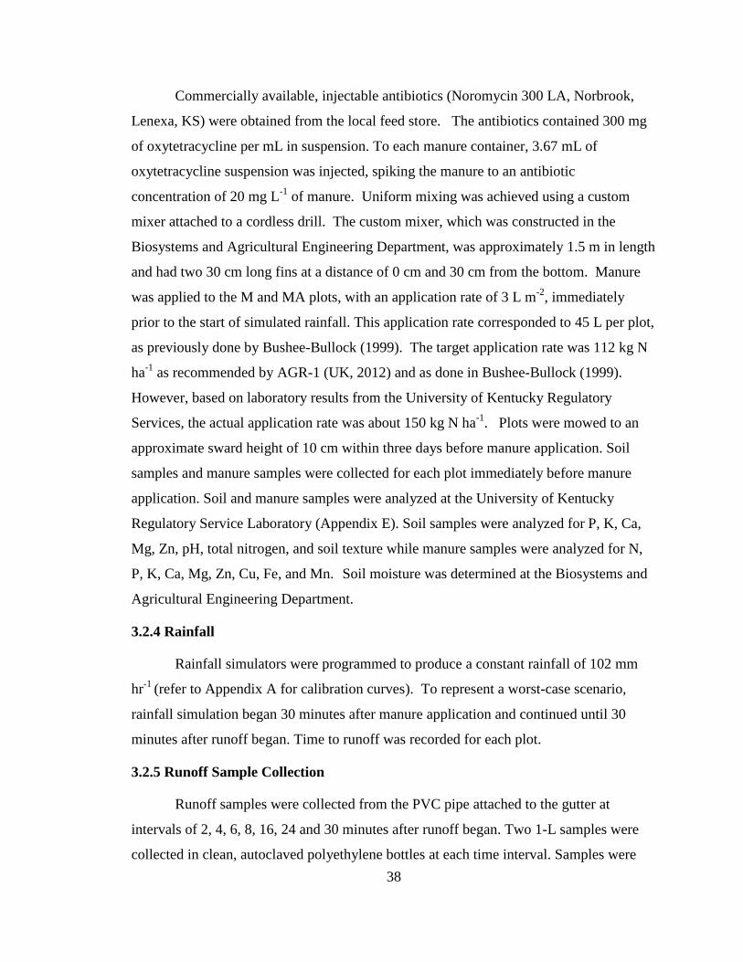
38

Commercially available, injectable antibiotics (Noromycin 300 LA, Norbrook,

Lenexa, KS) were obtained from the local feed store. The antibiotics contained 300 mg

of oxytetracycline per mL in suspension. To each manure container, 3.67 mL of

oxytetracycline suspension was injected, spiking the manure to an antibiotic

concentration of 20 mg L-1

of manure. Uniform mixing was achieved using a custom

mixer attached to a cordless drill. The custom mixer, which was constructed in the

Biosystems and Agricultural Engineering Department, was approximately 1.5 m in length

and had two 30 cm long fins at a distance of 0 cm and 30 cm from the bottom. Manure

was applied to the M and MA plots, with an application rate of 3 L m-2

, immediately

prior to the start of simulated rainfall. This application rate corresponded to 45 L per plot,

as previously done by Bushee-Bullock (1999). The target application rate was 112 kg N

ha-1

as recommended by AGR-1 (UK, 2012) and as done in Bushee-Bullock (1999).

However, based on laboratory results from the University of Kentucky Regulatory

Services, the actual application rate was about 150 kg N ha-1

. Plots were mowed to an

approximate sward height of 10 cm within three days before manure application. Soil

samples and manure samples were collected for each plot immediately before manure

application. Soil and manure samples were analyzed at the University of Kentucky

Regulatory Service Laboratory (Appendix E). Soil samples were analyzed for P, K, Ca,

Mg, Zn, pH, total nitrogen, and soil texture while manure samples were analyzed for N,

P, K, Ca, Mg, Zn, Cu, Fe, and Mn. Soil moisture was determined at the Biosystems and

Agricultural Engineering Department.

3.2.4 Rainfall

Rainfall simulators were programmed to produce a constant rainfall of 102 mm

hr-1

(refer to Appendix A for calibration curves). To represent a worst-case scenario,

rainfall simulation began 30 minutes after manure application and continued until 30

minutes after runoff began. Time to runoff was recorded for each plot.


Runoff samples were collected from the PVC pipe attached to the gutter at

intervals of 2, 4, 6, 8, 16, 24 and 30 minutes after runoff began. Two 1-L samples were

collected in clean, autoclaved polyethylene bottles at each time interval. Samples were

39

collected for 60 seconds or until the bottle was filled, whichever came first. The time

required to fill each bottle and the bottle’s weight were recorded. An average tare weight

was obtained for all bottles prior to sample collection. These values were used to create

two flow-weighted composite samples for each plot. One sample was created for

bacterial analysis while the other was used for the remaining constituents. The data

collected and volumes of each timed sample were used to create the composite samples

(Appendix B).


All eight samples collected from each plot (seven timed intervals and one

composite) were tested for the following constituents: E. coli, oxytetracycline, NO3-N,

NH4-N, PO4-P, pH, EC, TSS, Cl, TOC and turbidity. Samples were stored at

approximately 4°C until analysis. The University of Kentucky’s Forestry Department

analyzed samples for NO2-N, NO3-N, NH4-N, PO4-P, Cl, and TOC. A Bran-Luebbe

Auto-Analyzer III (Norderstedt, Germany) was used for the analysis of NO3-N and NH4-

N. A Dionex Ion Chromatograph (Sunnyvale, California) was used for PO4-P, Cl, and

NO2-N. Total organic carbon (TOC) was analyzed using a Shimadzu Total Orgainic

Carbon Analyzer (Kyoto, Japan).

Analysis for E.coli, oxytetracycline, pH, EC, turbidity and TSS occurred at the

Biosystems and Agricultural Engineering Department. E.Coli analysis was conducted

within 6 hours of sample collection. Coliert-18 was purchased from IDEXX laboratories

(Westbrook, Maine). Each sample from plots receiving manure was diluted three times

using sterile deionized (DI) water and buffer water. Instructions for buffer water

preparation and dilution can be found in Appendix C. Samples from control plots were

only diluted once. All dilutions were analyzed for E.coli by dissolving one packet of

Coliert-18 and two drops of anti-foaming agent in the sample. The samples were poured

into a Quanti-Trays*/2000 and sealed using an IDEXX Quanti-Tray* Sealer. Trays were

placed in an incubator at 35°C±0.5°C for 18-22 hrs. A UV-light was used after

incubation to determine the number of cells that fluoresced and turned yellow, indicating

the presence of E.coli. Software provided by IDEXX was used to determine the most

40

probable number of E.coli in each sample based on the number of cells that were

positive. Averages of the values for each dilution of each sample were computed.

An EcoTestr-EC Low (Vernon Hills, Illinois) was used for EC analysis. A

Thermo Electron Corporation Orion 520A+ (Waltham, Massachusetts) was used for pH

determination and a LaMotte 2020 turbidimeter (Chestertown, Maryland) was used for

turbidity. If the sample was too turbid, a 1/10 dilution was done by adding 1 mL of

sample to 9 mL of DI water. TSS analysis was conducted using a Sequoia Scientific

LISST-Portable|XR (Bellevue, Washington). Samples (175 mL) were separately added

to the mixing chamber and the mixer turned on. If sample was to turbid, 100 ml was

removed and the remaining sample was diluted with100 mL of DI water. All analyses

were conducted per standard methods (APHA et al., 1998).


Samples were analyzed for antibiotics using the methodology described in

Appendix D that was developed in the Biosystems and Agricultural Engineering

Department by Dr. Manish Kulshrestha. Samples were centrifuged at 3,500 rpm for 20

minutes on Thermo Scientific Survall Legend XTR Centrifuge (Waltham, Massachusetts)

before adding 45 mL to a 50 ml glass test tube. Each test tube was covered with a

kimwipe and placed in SP Scientific VirTis Wizard 2.0 lyophilzer (Gardiner, New York)

until dry (approximately 3 days). The remaining residue was dissolved in 900 µL of 50%

methanol solution, giving a 50X concentration from the original sample. The solution

was centrifuged again at 4,000 rpm for 10 minutes. A known amount of oxytetracycline

was added to the solution to give a better defined peak on the HPLC. A 25X concentrated

sample was achieved by adding 100µL of 2 µg mL-1

oxytetracycline solution to 100 µL

of concentrated solution.

High-Pressure Liquid Chromatography (HPLC) was used to separate the analytes.

A gradient mobile phase of 0.5% acetic acid in water and 0.5% acetic acid in methanol

was used. A Dionex Ultimate 3000 HPLC (Sunnyvale, California) along with an Ultimate

3000RS Variable Wavelength detector set at 290 nm was used for this analysis. The

HPLC used a pumping rate of 0.400 mL min-1

and injected 20µL of sample through a

41

Dionex Acclaim 120 (C18) column (Sunnyvale, California). Four standards (10, 20, 100

and 200 µg mL-1

) were used for calibration.

3.2.7 Data Analysis

Runoff flow rates from each plot were variable; therefore, constituent

concentrations were normalized by flow rate. Differences between treatments were

assessed for oxytetracycline using linear mixed models (PROC MIXED) and least square

means (LSMEANS) in SAS 9.3. Pearson correlation coefficients (r) between

concentrations of oxytetracycline in runoff samples and the other constituents were

determined for each treatment using the PROC CORR. The Pearson correlation

coefficient measures the linear correlation between two variables and ranges between -1

and 1. Negative values indicate a negative correlation while positive indicate a positive

relationship. A significance level of α=0.05 was used fo all analyses.


3.3.1 Manure and Soil Sampling

Table 3.3 contains the manure sampling results for each treatment. Values for N

and P were similar to those reported by ASABE (2005) for flush building. Table 3.4

contains the soil sampling results for each treatment. Values for organic matter (OM) and

N differed between C and MA; P did not differ between the treatments. Results for OM

were similar to those reported by Edwards et al. (2000) who used plots at the same

rainfall facility. However, N and P levels in this study were much lower than those

reported by Edwards et al. (2000). Values of N and P in this study ranged between 827 to

1,009 mg kg-1

and 37 to 47 mg kg-1

for N and P, respectively while Edwards et al. (2000)

recorded mean N and P values of 3,547 mg kg-1

for N and 169 mg kg-1

for P from soils

prior to manure and urine application. The differences may be due to the lengthy fallow

period (~10 years) experienced by the plots.

42

Table 3.3. Manure Sampling Results.

Treatment1

C (%)2 N (%) P (%)

M

2.0±0.0 a 0.5±0.0 a 0.1±0.0 a

MA

2.0±0.2 a 0.5±0.0 a 0.1±0.0 a 1C=control, M=manure only, and MA=manure and antibiotics.

2C=carbon, N=nitrogen, P=phosphorus

3Within column means followed by the same letter are not significantly different (α=0.05).

Table 3.4. Soil Sampling Results.

Treatment1

OM (%)2 N (mg kg

-1) P (mg kg

-1)

C

2.8±0.2a3 824±52 a 43±12 a

M

3.3±0.2 ab 947±44 ab 53±11 a

MA

3.5±0.4 b 1,009±108 b 47±11 a 1C=control, M=manure only, and MA=manure and antibiotics.

2OM=organic matter, N=nitrogen, P=phosphorus

3Within column means followed by the same letter are not significantly different (α=0.05).

3.3.2 Antibiotic Losses via Runoff

Treatment (p<0.0001) and sampling interval (p=0.0113) had significant effects on

oxytetracyline concentrations while replication (p=0.4286) did not. As expected,

oxytetracycline concentrations for the MA treatment differed significantly from the M

and the C plots (Table 3.5). For all plots, oxytetracycline concentrations were highest at

the time intervals 2, 4 and 6 minutes after the start of runoff; concentrations decreased as

the simulated storm continued (Figure 3.1). Oxytetracycline, as well as most of the other

constituents, exhibited the first flush phenomenon, which refers to a disproportionally

high concentration of a constituent in runoff during the first part of a storm (Sansalone

and Buchberger, 1997). This first-flush phenomenon is often seen in runoff events with

Table 3.5 Flow Normalized Oxytetracylcine Levels per Treatment.

Treatment1

Mean Concentration (µg·s L-2

)2,3

C

378.2b

M

421.7b

MA

1897.3a

1C=control, M=manure only, and MA=manure and antibiotics.

2Treatments with the same superscript indicate the means were not significantly different (p<0.05).

3Non-normalized means are as follows: C= 15.6 µg L

-1, M= 22.5 µg L

-1, and MA=129.7 µg L

-1.

43

Time Since Start of Runoff (min)

0 5 10 15 20 25 30 35

Oxy

tetr

acyc

line

(g

·s L

-2)

0

1000

2000

3000

4000

5000

Figure 3.1. Oxytetracycline Concentrations Normalized by Flowrate for a MA Plot (B6).

44

both suspended and dissolved constituents (Sansalone and Buchberger, 1997; Braskerud,

2002).

While it was expected that the C and M plots would not have detectable

oxytetracycline levels, this was not the case. The initial time intervals (2, 4 and 6

minutes) for the C and M plots produced higher than expected means (Figures 3.2 and

3.3). At the 8 minute and subsequent intervals, oxytetracycline levels plateaued,

approaching zero or nearly zero for most plots. The higher oxytetracylcine

concentrations in the C and M plots, at the beginning of the simulated storm events, were

attributed to difficulties in achieving peak separation in the chromatograms produced by

the HPLC at these low concentrations. Challenges in achieving peak separations in

samples could account for a portion of the oxytetracycline levels as concentrations are

computed based on the areas under the curves. Also important to note is that the samples

from the M, as well as MA, plots contained manure particles and hence organic matter.

The presence of organic matter has been shown to negatively impact oxytetracycline

recovery rates (Yang et al., 2005). In the runoff samples, another unknown pollutant was

detected near the peak of oxytetracycline thus preventing the return of the measurement

line to the datum. This had a greater impact on the samples from the M plots. This

interference made quantification of low levels of oxytetracycline difficult. It is possible

that concentrating the samples via lyophilization did not allow for the removal of the

interfering pollutant. Hirsch et al. (1998) found an average oxytetracyline recovery rate

of 108% for spiked spring water when using a similar lyophilization technique; however,

recovery rates decreased to 49% in the presence of high organic matter.

The peak (unnormalized) concentrations of oxytetracycline ranged between 62 and 549

µg L-1

for the four MA plots. Three of the four peaks (144, 408, and 549 µg L-1

) were

much higher than those found in other runoff studies. Kay et al. (2005) in the United

Kingdom, applied swine manure with an oxytetracycline concentration of 18.85 mg L-1

to

runoff plots and measured a peak runoff concentration of 71.7 µg L-1

. Manure was

applied 24 hrs before irrigation, which would have allowed the antibiotics to infiltrate

into the soil before the simulated storm event. The plots only received 15 mm of rain

over the course of two days, which did not allow for as much runoff to be generated as

quickly as in this study. Dolliver and Gupta (2007) measured antibiotic losses

45


0 5 10 15 20 25 30 35

Oxy

tetr

acyc

line

(g

·s L

-2)

0

50

100

150

200

250

300

350

Figure 3.2. Oxytetracycline Concentrations Normalized by Flowrate for a C Plot (C2).

46


0 5 10 15 20 25 30 35

Oxy

tetr

acyc

line

(g

·s L

-2)

50

60

70

80

90

100

110

120

Figure 3.3. Oxytetracycline Concentrations Normalized by Flowrate at M Plot (B4).

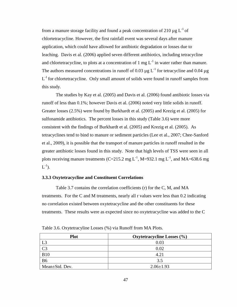
47

from a manure storage facility and found a peak concentration of 210 µg L-1

of

chlortetracycline. However, the first rainfall event was several days after manure

application, which could have allowed for antibiotic degradation or losses due to

leaching. Davis et al. (2006) applied seven different antibiotics, including tetracycline

and chlortetracycline, to plots at a concentration of 1 mg L-1

in water rather than manure.

The authors measured concentrations in runoff of 0.03 µg L-1

for tetracycline and 0.04 µg

L-1

for chlortetracycline. Only small amount of solids were found in runoff samples from

this study.

The studies by Kay et al. (2005) and Davis et al. (2006) found antibiotic losses via

runoff of less than 0.1%; however Davis et al. (2006) noted very little solids in runoff.

Greater losses (2.5%) were found by Burkhardt et al. (2005) and Krezig et al. (2005) for

sulfonamide antibiotics. The percent losses in this study (Table 3.6) were more

consistent with the findings of Burkhardt et al. (2005) and Krezig et al. (2005). As

tetracyclines tend to bind to manure or sediment particles (Lee et al., 2007; Chee-Sanford

et al., 2009), it is possible that the transport of manure particles in runoff resulted in the

greater antibiotic losses found in this study. Note that high levels of TSS were seen in all

plots receiving manure treatments (C=215.2 mg L-1

, M=932.1 mg L-1

, and MA=638.6 mg

L-1

).

3.3.3 Oxytetracycline and Constituent Correlations

Table 3.7 contains the correlation coefficients (r) for the C, M, and MA

treatments. For the C and M treatments, nearly all r values were less than 0.2 indicating

no correlation existed between oxytetracycline and the other constituents for these

treatments. These results were as expected since no oxytetracycline was added to the C

Table 3.6. Oxytetracyline Losses (%) via Runoff from MA Plots.

Plot Oxytetracycline Losses (%)

L3 0.03

C3 0.02

B10 4.21

B6 3.5

Mean±Std. Dev. 2.06±1.93

48

Table 3.7. Pearson Correlation Coefficients (r) between Oxytetracycline Concentrations

and Constituent Concentrations for C and M Treatments.1

Constituents Plots

C M MA

E.coli -0.199 0.112 0.6902

Cl- 0.026 -0.025 0.717

2

PO4 0.273 0.029 0.192

NO3-N 0.024 -0.065 -0.006

NH4-N 0.126 -0.144 0.6712

TOC 0.180 -0.122 0.5932

pH 0.107 0.6592 0.298

EC 0.167 0.110 0.5862

Turbidity -0.018 -0.192 0.5032

TSS 0.179 0.3772 0.515

2

1 All concentrations were flow-normalized.

2Significant at α=0.05 level.

and M plots. For the M plots, the correlation coefficients between oxytetracycline and

pH and TSS were substantially higher. With regards to TSS, this finding could indicate

that higher levels of manure particles, and therefore organic matter and pH, could have

effected oxytetracycline levels (Yang et al., 2005).

For the MA plots, the majority of the measured constituents were significantly

correlated to oxytetracycline (Table 3.5). As seen in Figures 3.4 to 3.6, pH, NO3-N, and

PO4, respectively, exhibited no relationship with oxytetracycline. With regards to pH, the

range of recorded values was small (7.0-7.7), and the presence of manure in the MA plots

did not affect pH levels. For NO3-N, several samples (71%) with levels below the

detection limit, an aspect that could have accounted in part for the lack of correlation with

oxytetracycline, occurred in the MA plots. PO4 also had a number of samples with non-

detectable values (43%) in the MA plots.

For the MA plots, all other constituents were significantly and positively

correlated with oxytetracycline (Table 3.5). In all instances, correlation coefficients were

above 0.5. Chloride exhibited the strongest correlation to oxytetracycline (r=0.72), as

seen Figure 3.7. The reason for this strong relationship is unclear. The label for

49

Oxytetracycline ( g·s L-2

)

0 2000 4000 6000 8000

pH

(p

H u

nits·s

L-1

)

0

100

200

300

400

500

Figure 3.4. Relationship between Oxytetracycline and pH for the MA Plots.

50


)

0 2000 4000 6000 8000

NO

3-N

(m

g·s

L-2

)

0

10

20

30

40

Figure 3.5. Relationship between Oxytetracycline and NO3-N for the MA Plots.

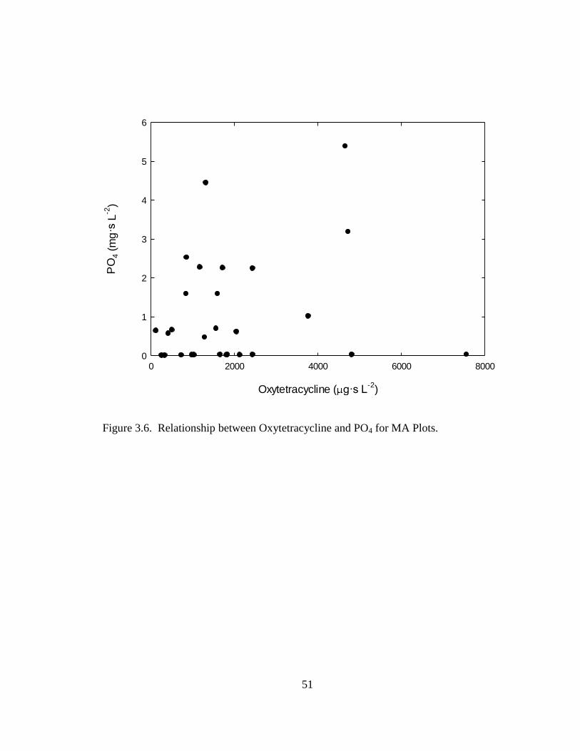
51


)

0 2000 4000 6000 8000

PO

4 (

mg

·s L

-2)

0

1

2

3

4

5

6

Figure 3.6. Relationship between Oxytetracycline and PO4 for MA Plots.

52


0 5 10 15 20 25 30 35

E.c

oli

(cfu

·s L

-2)

-10000

0

10000

20000

30000

40000

50000

M

MA

Figure 3.7. E. coli Concentrations for M and MA Plots During the Simulated Storm

Events.

53

Noromycin 300 LA indicates that hydrochloric acid could have been used in production

of the antibiotic to adjust the pH. Interestingly, the correlation coefficient between

oxytetracycline and E.coli indicates a strong positive correlation (r=0.69). Since

oxytetracycline is used to kill bacteria such as E. coli, it was theorized that higher levels

of oxytetracycline in runoff would result in lower levels of E. coli; however, this was not

the case (Figure 3.7).

The constituents TOC, EC, TSS and NH4-N also displayed strong positive

correlations with oxytetracylcine concentrations (Figures 3.8-3.11). The relationship

between TOC and oxytetracycline was expected as both are organic compounds. The

relationships between TSS and oxytetracycline and turbidity and oxytetracycline indicate

that the antibiotics are correlated with the amount of solids in the samples, a phenomenon

noted by Loke et al. (2002). Kulthrestha et al. (2004) noted the likelihood of

oxytetracycline to bind to clays with high ammonium content, which could account for

the strong correlation between ammonia and oxytetracycline seen in this study.

3.3.4. Best Management Practice Selection

Due to the common usage of antibiotics in livestock coupled with the

unlikelihood that significant forms of source reduction will occur in the foreseeable

future, other types of BMPs (e.g. structural) are needed to reduce the transport of

antibiotics to waterways. The results of this study suggest that BMPs which target

particulates or sediments may be more appropriate for reducing the transport of

oxytetracycline and potentially other antibiotics. Davis et al. (2006) concluded erosion

control practices could aid in the reduction of antibiotics in runoff. A similar sentiment

was echoed by Lin et al. (2011) who measured a 75% reduction in the transport of two

antibiotics, tysolin and enrofloxacin, with the use of a 4 m vegetative buffer strip. Other

BMPs such as composting and chemical additives could also aid in the reduction of off-

field transport of antibiotics. Arikan et al. (2007) showed a 99% removal of extractable

oxytetracycline in cattle manure after composting for 35 days. Chemical additives are

commonly used by the wastewater treatment industry, but their potential for reducing

antibiotic transport has received little research. Punamiya et al. (2013) found that

aluminum-based water treatment residuals have high potential to bind to tetracycline

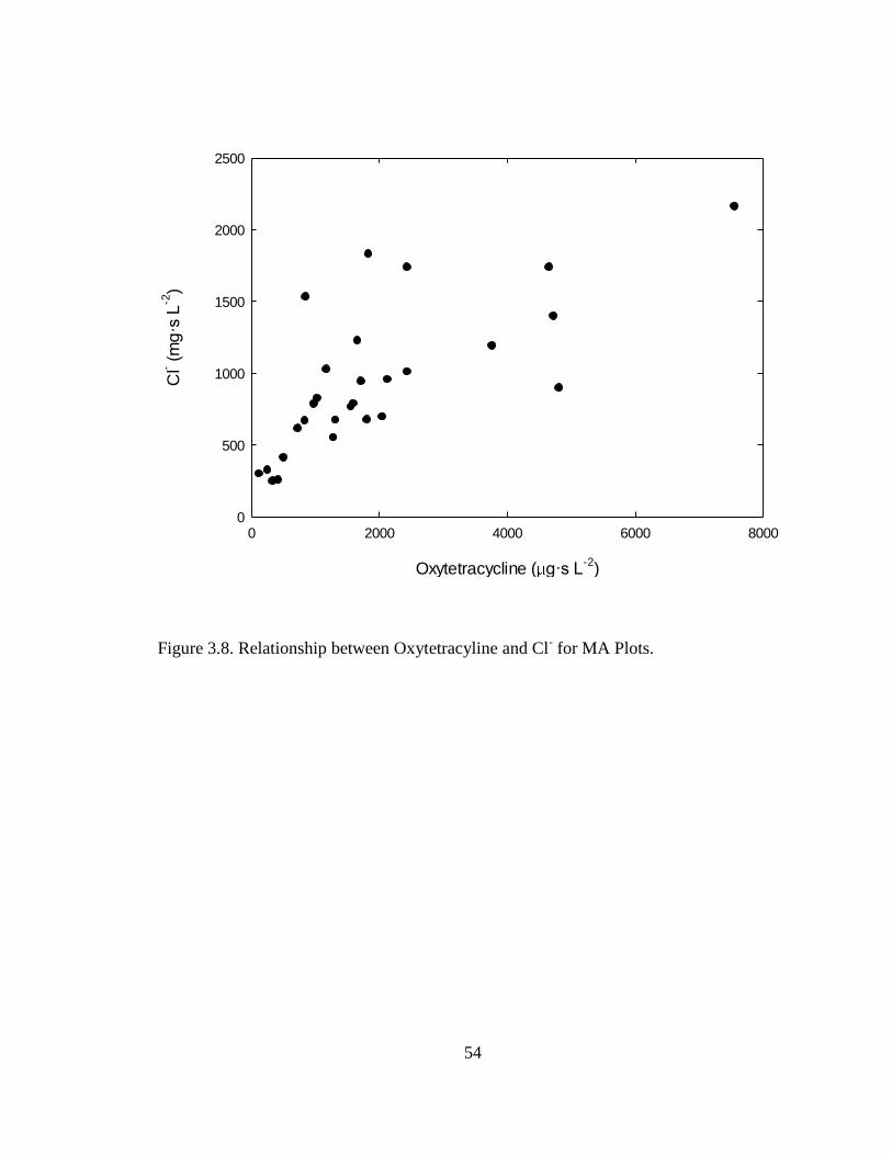
54


)

0 2000 4000 6000 8000

Cl- (

mg

·s L

-2)

0

500

1000

1500

2000

2500

Figure 3.8. Relationship between Oxytetracyline and Cl- for MA Plots.

55


)

0 2000 4000 6000 8000

TO

C (

mg

·s L

-2)

0

1000

2000

3000

4000

5000

Figure 3.9. Relationship between Oxytetracycline and TOC for MA Plots.

56


)

0 2000 4000 6000 8000

EC

0

5000

10000

15000

20000

25000

30000

35000

Figure 3.10. Relationship between Oxytetracycline and EC for MA Plots.

57


)

0 2000 4000 6000 8000

Turb

idity

(NT

U·s

L-1

)

0

2000

4000

6000

8000

10000

12000

14000

Figure 3.11. Relationship between Oxytetracycline and Turbidity MA Plots.

58

antibiotics. Another aluminum-based compound, aluminum sulfate or alum, has been

used for a number of years as a flocculent to settle out solids and remove organic

compounds from wastewater. Alum is also used by the livestock industry, particularly

poultry producers, to reduce the transport of phosphorus (DeLuane and Moore, 2013).

The strong correlation between oxytetracycline and the constituents TSS, turbidity and

TOC suggests a BMP, such as a vegetative buffer strip or alum, may be a viable method

for reducing the transport of this antibiotic.

3.4 CONCLUSIONS

Veterinary antibiotics such as oxytetracycline can be transported to waterbodies

via overland flow. Studies have shown that oxytetracycline can undergo

photodegradation (Doi and Stoskopf, 2000; Xuan et al., 2010), however, for this to occur,

the transport rate of oxytetracyline must be reduced so that the exposure time to sunlight

is maximized. Results from this study show that the presence of oxytetracycline is

strongly correlated to the presence of other water quality constituents such as E.coli, Cl,

TOC, turbidity, and TSS. The strong correlation between oxytetracycline and measures

of suspended sediment, namely turbidity and TSS, coupled with the likelihood of

oxytetracycline binding to manure particles suggests that BMPs used to reduce solids in

runoff, such as vegetative buffer strips and flocculants, could potentially reduce the

transport of oxytetracycline as well.

59

CHAPTER 4: EFFECT OF ALUM ON SURFACE TRANSPORT OF

OXYTETRACYCLINE

4.1 INTRODUCTION

Antibiotics are used in livestock production for both therapeutic and subtherapeutic

uses. Subtherapeutic uses are mainly the prevention of the spread of diseases and the

promotion of livestock growth through the increased nutrient absorption by the animal

and less by gastrointestinal bacteria (LaShore and Pruden, 2009). The USEPA (2013)

estimates that 60-80% of livestock and poultry routinely receive antimicrobials through

feed, water, injections or external applications. An estimated 93% of grower/finisher

hogs were administered antibiotics at some point during the grower/finisher time (USDA,

1996) with 25% of swine facilities administering antibiotics as levels higher than

recommended (Dewey et al., 1997). One of the challenges associated with frequently

dosing livestock with antibiotics is that livestock can only partially metabolize the

antibiotics they are administered. Thus, livestock excrete antibiotics at high rates (30%-

90%) and in virtually unchanged forms from the parent compounds (Sarmah et al., 2006).

Antibiotics have been found in manures at concentrations ranging from trace levels to as

much as 200 mg L-1

(Kumar et al., 2005).

Many of the antibiotics approved for use in livestock are used in humans as well.

Oxytertracycline, a tetracycline class antibiotic, is approved by the Food and Drug

Administration for therapeutic uses in humans as well as livestock, and it is approved for

subtherapeutic uses in cattle and swine as a growth promoter. Tetracyclines are one of

the largest classes of antibiotics used in livestock and poultry. Over 70% of the

antibiotics administered to livestock and poultry are of the classes of tetracyclines and

ionophores (USEPA, 2013).

The main concern with such high rates of antibiotic administration to livestock is the

potential for the development of antibiotic-resistant strains of bacteria. While sampling

private groundwater supplies, McKeon et al. (1995) found that 90% of the over 250

coliforms and non-coliforms samples were resistant to at least one antibiotic with 78% of

these coliforms displaying resistance to multiple antibiotics. Chee-Sanford et al. (2001)

found tetracycline resistant genes in bacteria in groundwater sampled more than 250 m

60

downstream of a swine waste storage lagoon indicating that such bacteria are readily

transported.

Because of the frequent dual usage between humans and livestock coupled with the

fact that detection of antiobiotics in the environment is occurring more frequently

(USEPA, 2007), the USEPA has classified antibiotic as a contaminant of emerging

concern (CEC). A CEC is one that is now being detected in the environment and/or is at

higher than expected levels, meaning it was not previously present in the environment or

was present at undetectable or very low levels (USEPA, 2007). Land application of

manure, which is common with livestock operations, serves as the primary pathway for

antibiotics to enter waterbodies (Baguer et al., 2000; Arikan et al., 2008). Approximately

50% of surface waters may contain antibiotics (Koplin et al., 2002). But, as seen with

Chee-Sandford et al. (2001), antibiotics are not found in surface waters alone.

Campagnolo et al. (2002) also found antibiotics in groundwater near swine farms in Iowa

– a state with large amounts of karst (Veni et al., 2001). The authors noted that 31% of

ground and surface water samples collected near swine operations and 67% of ground

and surface water samples near poultry operations contained antibiotics. Such findings

are of particular importance in karstic environment where surface water and ground water

connections are strong meaning pollutants applied to the land can readily access aquifers.

Aluminum sulfate, or alum, is a non-toxic flocculent used in the wastewater industry

(Tchobanoglous et al., 2003; Mason et al., 2005) and the poultry industry (Moore and

Miller, 1994; DeLuane and Moore, 2013). Numerous studies have demonstrated the

effectiveness of alum to reduce phosphorus levels in runoff (Moore and Miller, 1994;

Edwards and Daniel, 1993; Edwards et al., 1999; Smith et al., 2001; Penn and Bryant,

2006). Essentially, soluble forms of phosphorus are converted to insoluble ones which

are then precipitated out. Alum can also reduce concentrations of arsenic (56%), copper

(44%), and zinc (36%) (Moore et al., 1998) as well as the hormone 17β-estradiol

(DeLaune and Moore, 2013). Only one study has examined the potential use of alum to

reduce antibiotic transport. Adams et al. (2002), in a lab-scale study, examined the

effectiveness of alum to reduce antibiotic concentrations in river water. The authors

examined seven antibiotics, six of which were sulfidimides class of antibiotics; the other

was in the carbadox class. Results of the study indicated that alum did not remove a

61

significant amount of antibiotics from the river water. Tetracyclines, however, behave

differently than sulfidimides and carbadox classes of antibiotics as tetracyclines have a

higher tendency to bind to manure particles (Loke et al., 2002). The tendency of a

pollutant to bind to soil particles is described by the sorption coefficient, Kd, which is a

ratio of the amount of chemical sorbed to soil to the amount that is still in solution (Brady

and Weil, 2008). Higher Kd values mean the pollutant is more likely to bind to soil

particles. Sulfidimides, such as those studied by Adams et al. (2002, have low Kd values

(0.6-4.9) as compared to tetracyclines which have high Kd values (420-1030) (Tolls,

2001). Punamiva et al. (2013) noted that aluminum water treatment residuals, part of the

waste product from the water purification process, can sorb to tetracyclines thus

removing them from aqueous solution. The authors found a removal rate of 98% for

tetracycline and a 96% for oxytetracycline. Thus, the objective of this study was to

examine the effectiveness of alum for reducing concentrations of tetracycline antibiotic

(oxytetracycline) in simulated runoff.


4.2.1 Study Site

This study was conducted at the rainfall simulation facility at the University of

Kentucky’s Maine Chance Research farm (latitude: 38.1164°N; longitude: 84.4903W).

The facility consists of three rainfall simulators, which were constructed as described in

Miller (1987). Fescue plots measuring 2.44 m by 6.10 m were constructed on Maury silt

loam (fine, mixed, mesic Typic Paleufalf) (NRCS, 2013) as described by Edwards et al.

(2000) and planted with Kentucky 31 fescue. Each plot was bordered by galvanized steel

and was equipped with a gutter at the base that diverted runoff in to a PVC pipe located

in a sump. A wood cover was placed over the gutter to ensure that only runoff was

collected during the sampling events.


Rainfall simulators were used to generate curve numbers (CNs) for each plot

(Appendix A). Sixteen plots with similar CNs were selected for use in this study (Table

4.1). Plots selected for this study had a mean curve number of 83 ±4.

62

Table 4.1 Curve Numbers of Plots Used in the Study.

Plot CN Plot CN

B1 82 C5 89

B4 82 C6 77

B5 88 D1 86

B6 90 D5 84

B10 82 L1 84

C2 89 L3 79

C3 82 N2 77

C4 80 N9 81

4.2.3 Experimental Treatments

Liquid swine manure was obtained from a private hog farm in Bardstown, KY.

Manure was collected from hogs that had not been administered antibiotics since birth.

The manure had a slurry consistency, and it was stored in a pit prior to collection for this

study. Collected manure was stored in a 1,040 L polyethylene intermediate bulk

container (IBC) tote at the University of Kentucky Biosystems and Agricultural

Engineering Department.

Four treatments were randomly assigned to the plots (Table 4.2). Treatments

included a control (manure was not applied) (C), manure only (M), manure plus

antibiotics (MA), and manure plus antibiotics and alum (MAA). Manure (55L) was

placed in separate 208 L barrels which were designated in accordance with treatment to

prevent cross-contamination. Manure for each treatment receiving antibiotics was spiked

to a concentration of 20 mg L-1

by adding 3.67 mL of oxytetracycline to the 55 L of

manure. The oxytetracycline (Noromycin 300 LA, Norbrook, Lenexa, KS) was a

commercially available, injectable form containing 300 mg of antibiotic per mL in

suspension. For the MAA treatment, 1.13 L of liquid alum (48.5% solution) was added

to the manure and antibiotics resulting in a 1% alum concentration (Bushee-Bullock,

1999; Smith et al., 2001). Prior to application to the plots, manure was mixed for 5

minutes using a custom built mixer attached to a drill. The custom mixer, which was

constructed in the Biosystems and Agricultural Engineering Department, was

approximately 1.5 m in length and had two 30 cm long fins at a distance of 0 cm and 30

cm from the bottom.

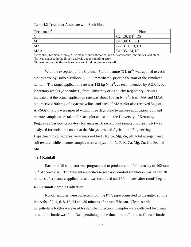
63

Table 4.2 Treatment Associate with Each Plot.

Treatment1 Plots

C C2, C6, D12, D5

M B4, B83 C5, L1

MA B6, B10, C3, L3

MAA B1, B5, C4, N9 1C=control, M=manure only, MA=manure and antibiotics, and MAA=manure, antibiotics, and alum.


3B8 was not used in the analysis because it did not produce runoff.

With the exception of the C plots, 45 L of manure (3 L m-2

) was applied to each

plot as done by Bushee-Bullock (1999) immediately prior to the start of the simulated

rainfall. The target application rate was 112 kg N ha-1

, as recommended by AGR-1, but

laboratory results (Appendix E) from University of Kentucky Regulatory Services

indicate that the actual application rate was about 150 kg N ha-1

. Each MA and MAA

plot received 900 mg of oxytetracycline, and each of MAA plot also received 54 g of

Al2(SO4)3. Plots were mowed within three days prior to manure application. Soil and

manure samples were taken for each plot and sent to the University of Kentucky

Regulatory Service Laboratory for analysis. A second soil sample from each plot was

analyzed for moisture content at the Biosystems and Agricultural Engineering

Department. Soil samples were analyzed for P, K, Ca, Mg, Zn, pH, total nitrogen, and

soil texture, while manure samples were analyzed for N, P, K, Ca, Mg, Zn, Cu, Fe, and

Mn.

4.2.4 Rainfall

Each rainfall simulator was programmed to produce a rainfall intensity of 102 mm

hr-1

(Appendix A). To represent a worst-case scenario, rainfall simulation was started 30

minutes after manure application and was continued until 30 minutes after runoff began.


Runoff samples were collected from the PVC pipe connected to the gutter at time

intervals of 2, 4, 6, 8, 16, 24 and 30 minutes after runoff began. Clean, sterile

polyethylene bottles were used for sample collection. Samples were collected for 1 min

or until the bottle was full. Data pertaining to the time to runoff, time to fill each bottle,

64

and weight of each bottle were recorded (Appendix B). All bottles were weighed before

sample collection and an average tare weight was calculated. Two flow-weighted

composite samples, one for bacterial analysis and one for the analysis of all other

constituents, were created using the weight of each sample along with the respective

sample bottle fill times. The data used to create the composite samples are presented in

Appendix B.


For each plot, samples from the seven time intervals along with a composite were

analyzed for E. coli, oxytetracycline, NO3-N, NH4-N, PO4-P, pH, EC, TSS, Cl, TOC and

turbidity. Samples were stored at approximately 4°C until analysis. Analysis for NO3-N,

NH4-N, PO4-P, Cl, and TOC occurred at the University of Kentucky’s Forestry

Department. A Bran-Luebbe Auto-Analyzer III (Norderstedt, Germany) was used for the

analysis of NO3-N and NH4-N. A Dionex Ion Chromatograph (Sunnyvale, California)

was used for PO4-P, Cl, and NO2-N. Total Organic Carbon (TOC) was analyzed using a

Shimadzu Total Orgainic Carbon Analyzer (Kyoto, Japan).

Samples were analyzed for E. coli, oxytetracycline, pH, EC, turbidity, and TSS at

the University of Kentucky’s Biosystems and Agricultural Engineering Department. E.

coli analysis was conducted within 6 hours of sample collection using Coliert-18

purchased from IDEXX laboratories (Westbrooke, Maine) (Appendix C). EC was

determined using an EcoTestr-EC Low (Vernon Hills, Illinois). A Thermo Electron

Corporation Orion 520A+ (Waltham, Massachusetts) was used for pH determination, and

a LaMotte 2020 turbidimeter (Chestertown, Maryland) was used for turbidity. TSS

analysis was conducted using a Sequoia Scientific LISST-Portable|XR (Bellevue,

Washington). All analyses were conducted per standard methods (APHA et al., 1998).


Samples were analyzed for antibiotics using a methodology developed in the

Biosystems and Agricultural Engineering Department by Dr. Manish Kulshrestha. A

detailed description of antibiotic analysis can be found in Appendix D. Approximately 50

mL of sample was centrifuged at 3,500 rpm for 20 minutes in a Thermo Scientific Survall

Legend XTR Centrifuge (Waltham, Massachusetts), and 45 mL was added to a glass test

65

tube. Kimwipes were uses to cover the test tubes, before placing the samples in a SP

Scientific VirTis Wizard 2.0 lyophilzer (Gardiner, New York) until dry. After

approximately three days, the test tubes were removed from the lyophilizer and the dry

residue was dissolved in 900 µL of 50% methanol solution. This concentrated the

original sample 50X. The solution was transferred to microcentrifuge tubes and

centrifuged again at 4,000 rpm for 10 minutes with a Fisher Scientific Marathon 21000

(Waltham, Massachusetts). In order to achieve a better defined peak and to ensure the

right peak was selected, a known amount of oxytetracycline was added to each sample.

A 25X concentrated sample was achieved by adding 100 µL of 2 µg/mL oxytetracycline

solution to 100 µL of concentrated solution.

High-pressure liquid chromatography (HPLC) was used to separate the analytes.

A Dionex Ultimate 3000 HPLC (Sunnyvale, California) along with an Ultimate 3000RS

Variable Wavelength detector set at 290 nm (Kay et al., 2005) was used for this analysis.

Using a gradient mobile phase of 0.5% acetic acid in water and 0.5% acetic acid in

methanol, samples were ran through a Dionex Acclaim 120 (C18) column (Sunnyvale,

California). The HPLC injected 20µL of sample through the column and used a pumping

rate of 0.400 mL/min. Four calibration standards ranging from 10µg mL-1

to 200µg mL-1

were used.

4.2.7 Data Analysis

Runoff flow rates from each plot were variable; therefore, constituent

concentrations were normalized by flow rate. Differences between treatments and time

intervals were assessed using linear mixed models (PROC MIXED) and least square

means (LSMEANS) in SAS 9.3. All data were ln transformed to normalize the data.


4.3.1 Treatment Effects

Treatments did not significantly affect constituent concentrations for Cl, TOC,

pH, EC, turbidity, and TSS, but significant treatment effects were noted for E. coli, NO3-

N, NH4-N, PO4, and oxytetracycline (Table 4.3). The lack of significance with regards to

66

Table 4.3. Statistics for Runoff Variables (Mean ± Standard Deviation).

Constituent Treatment

1,2

C M MA MAA

ln E. coli (cfu·s L-2

) 7.9±1.9b 3

14.4±1.6a

14.5±2.0a

13.1±3.2a

ln Cl (mg·s L-2

) 6.4±1.4a

6.9±0.7a

6.9±0.6a

6.6±1.3a

ln NO3-N (mg·s L-2

) 1.9±1.5a

-1.7±1.9b

-1.5±2.3b

0.5±3.9ab

ln NH4-N (mg·s L-2

) 2.9±1.4b

5.7±0.8a

5.2±0.8a

5.2±0.9a

ln PO4 (mg·s L-2

) -4.0±1.8b

-0.8±2.6a

-1.6±2.4a

-1.9±1.9a

ln TOC (mg·s L-2

) 5.5±1.2a

6.6±1.0a

6.2±0.7a

6.4±1.2a

ln Oxytetracycline (µg·s L-2)

5.8±1.0

b 5.6±1.1

b 7.1±0.9

a 7.7±1.0

a 2

ln pH (pH units·s L-1

) 5.4±1.3a

4.7±0.9a

4.8±0.8a

5.5±1.7a

ln EC (µS·s L-1

) 9.4±1.1a

9.4±0.7a

9.3±0.6a

9.9±1.3a

ln Turbidity (NTU·s L-1

) 5.7±1.7a

7.7±1.1a

6.9±1.1a

7.2±0.8a

ln TSS (mg·s L-2

) 8.5±1.3a

9.4±1.0a

9.1±0.8a

9.6±0.8a

1C=control, M=manure only, MA=manure and antibiotics, and MAA=manure, antibiotics, and alum.

2Values computed for all time intervals and repetitions. All reported values were normalized by flow and

ln transformed. 3Different letters within rows indicated means differed statistically at α=0.05.

4At α=0.10 means for flow-normalized oxytetracyline were statistically greater for the MAA treatment than

for the MA (p=0.062).

the constituents Cl, TOC, EC, turbidity, and TSS was surprising as it was expected that

constituent levels would be highest for the M, MA and MAA plots and lowest for the C

plots. This lack of significance is due in part to the large amount of variation amongst the

plots and across the time intervals. While no significant repetition differences were

noted, significant time interval differences were found.

4.3.1.1 Non-significant Constituents

Levels of Cl were the same across all treatments considering all time intervals and

repetitions (Figure 4.1). This result was surprising considering that swine manure has

been shown to have Cl levels above 1,700 mg L-1

(Krapac et al., 2002). Only three of the

samples collected during the study had Cl levels above secondary drinking water

standards (250 mg L-1

), and all of these samples occurred in the M plots within the 2 and

4 minute time intervals. The use of chlorinated water from a municipal water supply as

the simulated rain consisted could have influenced Cl levels in runoff to some degree.

The lack of difference between treatments regarding TOC was also surprising

given the high levels of TOC in swine manure. Huang et al. (2006) noted that TOC

67

Time Since Runoff (min)

0 5 10 15 20 25 30 35

ln C

l (m

g·s

L-2

)

3

4

5

6

7

8

9

10

M

MA

MAA

C

Figure 4.1. Flow Normalized ln Cl Concentrations for Each Treatment. C=Control,


Alum.

68

accounted for about 37% of swine manure from a swine facility in Hong Kong. As such,

it was expected that the application of swine manure to the non-C plots would increase

TOC levels in runoff. Though not significantly different, TOC values for the C plots

were less than the M, MA and MAA plots for the first half of the simulated storm event

(Figure 4.2).

With regards to pH and EC, it was expected that the addition of manure would

increase pH and EC levels; however, this was not the case (Figures 4.3 and 4.4).

Edwards and Daniel (1993) recorded a pH from swine manure of 8.4 while Huang et al.

(2006) recorded an average value of 8.1. The average pH of runoff from this study was

lower for all treatments (7.4-7.6) than those values. The average pH level of 7.3 reported

by the municipal water supplier indicated that the rainfall used in this study was a greater

influence on runoff pH then the addition of manure, antibiotics and/or alum. And like

pH, average EC levels in runoff (429-890 µS cm-1

) largely reflected the values consistent

with those expected from the municipal water supplier given the limestone geology of the

region. Edwards and Daniel (1993) recorded EC values for swine manure of 19,500 µS

cm-1

while Krapac et al. (2002) recorded EC values over 30,000 µS cm-1

Sediment measures, TSS and turbidity were also not significantly different among

treatments though mean values for the C plot time intervals were lowest (Figures 4.5 and

4.6). Mean TSS values for the treatments ranged from 194 to 920 mg L-1

, across all

repetitions and time intervals, while for turbidity those values ranged from 12 to 381

NTU. These values were notably higher than those reported by Edwards and Daniel

(1993) who measured TSS values between 8 and 74 mg L-1

for a simulated rainfall study

with swine manure. The rainfall intensity used by the authors of 10 cm h-1

is the same

rate used in this study. The authors found that greater application rates of swine manure

resulted in higher levels of TSS in runoff. A similar trend was noted in this study

between the C plots and the M, MA and MAA plots though the trend was not significant.

4.3.1.2 Significant Constituents

Levels of E. coli were significantly lower for the C plots as compared to the M,

MA and MAA plots (Figure 4.7). The addition of manure to these plots increased E. coli

levels in runoff, as expected. Though the values for the MAA plots were lower than the

69


0 5 10 15 20 25 30 35

ln T

OC

(m

g·s

L-2

)

3

4

5

6

7

8

9

M

MA

MAA

C

Figure 4.2. Flow Normalized ln TOC Concentrations for Each Treatment. C=Control,


Alum.

70


0 5 10 15 20 25 30 35

ln p

H (

pH

units·s

L-1

)

3

4

5

6

7

8

9

M

MA

MAA

C

Figure 4.3. Flow Normalized ln pH Concentrations for Each Treatment. C=Control,


Alum.

71


0 5 10 15 20 25 30 35

ln E

C (

S·s

L-1

)

7

8

9

10

11

12

13

M

MA

MAA

C

Figure 4.4. Flow Normalized ln EC Concentrations for Each Treatment. C=Control,


Alum.

72


0 5 10 15 20 25 30 35

TS

S (

mg

·s L

-2)

5

6

7

8

9

10

11

12

M

MA

MAA

C

Figure 4.5. Flow Normalized ln TSS Concentrations for Each Treatment. C=Control,


Alum.

73


0 5 10 15 20 25 30 35

Turb

idity

(NT

U·s

L-1

)

2

3

4

5

6

7

8

9

10

M

MA

MAA

C

Figure 4.6. Flow Normalized ln Turbidity Concentrations for Each Treatment.


Antibiotics and Alum.

74


0 5 10 15 20 25 30 35

ln E

.co

li (

cfu

·s

L-2

)

2

4

6

8

10

12

14

16

18

20

M

MA

MAA

C

Figure 4.7. Flow Normalized ln E. coli Concentrations for Each Treatment. C=Control,


Alum.

75

M and MA plots, the addition of alum did not significantly decrease E. coli levels. The

lack of significant effect of alum on E. coli levels is surprising given that alum has been

used as a flocculent to remove bacteria from water. Bulson et al. (1984) reported that

over 90% of E. coli in lake water were removed by the addition of 15 mg L-1

of alum.

While the study by Bulson et al. (1984) allowed for a longer flocculation time than this

study (30 h vs 12-24 h), it was expected that the addition of alum, which was at a much

greater concentration (1 g L-1

) in this study, would reduce E. coli levels.

With regards to NO3-N, mean levels were highest for the C and MAA plot and

lowest for the M and MA plots (Figure 4.8). The reason for these differences is not

known. Krupac et al. (2002) noted that the swine manure used in their study had NO3-N

levels less than 0.2 mg L-1

with the majority of N in the form of NH3-N and organic N.

Edwards and Daniel (1993) measured low levels (0.1 mg L-1

) of NO3-N in runoff from

plots with swine manure. Hence the addition of swine manure to the plots was not

expected to increase NO3-N levels substantially. For NH4-N, mean concentrations were

lowest with the C plots as compared to the M, MA and MAA plots (Figure 4.9). Edwards

and Daniel (1993) noted a similar trend between control plots and those to which

manure was applied. The addition of manure to the plots in this study significantly

increased NH4-N levels, as expected since the swine manure used in this study contained

about 0.5% N (Appendix E). ASABE (2005) indicates that swine manure, such as that

used in this study, generally contains 0.14% NH3-N. Krupac et al. (2002) measured

average NH3-N levels of 4,380 mg L-1

in swine manure.

Levels of PO4 were lowest in the C plots as compared to the M, MA and MAA

plots (Figure 4.10). The addition of manure increased PO4 levels in runoff; however, the

addition of alum did not decrease PO4 levels as expected based upon prior alum research

related to poultry litter and phosphorus reductions in runoff (Moore and Miller, 1994;

Moore et al., 1999; Smith et al. 2001). The pH of the runoff (7.4-7.6) was within the

range of Al(OH)3 floc formations whereby PO4 is sorbed to the floc (Cooke et al., 1986;

Moore and Miller, 1994). It is possible that the alum dosage (1%) was too low to

promote significant PO4-P removal or that the Al(OH)3 flocs were transported with the

runoff.

76


0 5 10 15 20 25 30 35

ln N

O3-N

(m

g·s

L-2

)

-40

-20

0

20

40

60

80

100

120

140

160

M

MA

MAA

C

Figure 4.8. Flow Normalized ln NO3-N Concentrations for Each Treatment. C=Control,


Alum.

77


0 5 10 15 20 25 30 35

ln N

H4-N

(m

g·s

L-2

)

1

2

3

4

5

6

7

8

M

MA

MAA

C

Figure 4.9. Flow Normalized ln NH4-N Concentrations for Each Treatment. C=Control,


Alum.

78


0 5 10 15 20 25 30 35

ln P

O4 (

mg

·s L

-2)

-10

-8

-6

-4

-2

0

2

4

M

MA

MAA

C

Figure 4.10. Flow Normalized ln PO4-P Concentrations for Each Treatment. C=Control,


Alum.

79

A significant treatment effect was found for oxytetracycline. Both C and M plots

had lower concentrations of oxytetracycline as compared to MA and MAA plots (Figure

4.11). While MA and MAA plots did not differ at α=0.05, a significant difference was

noted at α=0.10. At this level of significance, MAA plots had higher concentrations of

oxytetracycline than MA plots. It was hypothesized that the alum may have precipitated

oxytetracycline, but that the particles were transported in runoff. If such were the case, a

second BMP such as a vegetated filter strip would be required. However, the lack of

significance, even at α=0.10 for the other constituents measured in this study suggests

that this was not the case. The ineffectiveness of alum in this study may have been

related to the alum dosage. Bushee-Bullock (1999) found no reduction in the transport of

the hormone 17β-estradiol at a 1% alum dosage; however, DeLuane and Moore (2013)

found reductions in 17β-estradiol using alum doses of 5%, 10% and 20%. On the other

hand, other contaminants in the swine manure may inhibit alum regardless of the dosage.

Choi et al. (2008) found that organic matter interfered in the removal efficiency of poly-

aluminum-chloride in the reduction of oxytetracycline in river water. Removal

efficiencies were reduced by 40% when river water samples had high organic matter

contents. The high organic matter contents of manure will likely require consideration if

alum is to be further explored for oxytetracycline removal.

4.3.2 Time Effects

A significant difference was noted with respect to time interval for all of the

examined constituents except NO3, PO4, and oxytetracycline (Table 4.4). The first flush

phenomenon, whereby a disproportionally high concentration occurs in runoff during the

first part of a storm (Sansalone and Buchberger, 1997; Braskerud, 2002), was seen with

the majority of examined constituents. The time interval 2 min had the highest

concentrations for all constituents. For the most part, constituent concentrations reached

a minimum level after either 16 to 24 min since the start of runoff. These results point to

the importance of the first 15 minutes of a storm event as this period of time is when the

greatest amounts of contaminants are typically transported to waterbodies (Soupir et al.,

2006; Kato et al., 2009; Delpla et al., 2011). As such, BMP selection should target

reductions of constituent losses during the early parts of the storm (Moore and Miller,

80


0 5 10 15 20 25 30 35

ln O

xyte

tra

cyc

line

(g

·s L

-2)

3

4

5

6

7

8

9

10

11

M

MA

MAA

C

Figure 4.11. Flow Normalized ln Oxytetracycline Concentrations for Each Treatment.


Antibiotics and Alum.

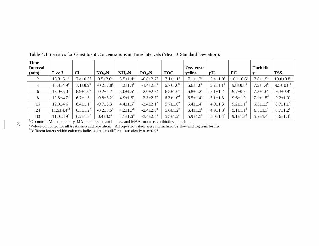
81

Table 4.4 Statistics for Constituent Concentrations at Time Intervals (Mean ± Standard Deviation).

Time

Interval

(min) E. coli Cl NO3-N NH4-N PO4-N TOC

Oxytetrac

ycline pH EC

Turbidit

y TSS

2 13.8±5.1a 7.4±0.8

a 0.5±2.6

a 5.5±1.4

a -0.8±2.7

a 7.1±1.1

a 7.1±1.3

a 5.4±1.0

a 10.1±0.6

a 7.8±1.5

a 10.0±0.8

a

4 13.3±4.9b 7.1±0.9

b -0.2±2.8

a 5.2±1.4

b -1.4±2.5

a 6.7±1.0

b 6.6±1.6

a 5.2±1.1

b 9.8±0.8

b 7.5±1.4

b 9.5± 0.8

b

6 13.0±5.0b 6.9±1.0

b -0.2±2.7

a 5.0±1.5

c -2.0±2.3

a 6.5±1.0

c 6.8±1.2

a 5.1±1.2

c 9.7±0.9

c 7.3±1.6

c 9.3±0.9

c

8 12.8±4.7b 6.7±1.3

c -0.8±3.2

a 4.9±1.5

c -2.3±2.7

a 6.3±1.0

d 6.5±1.4

a 5.1±1.3

c 9.6±1.0

c 7.1±1.5

d 9.2±1.0

c

16 12.0±4.6c 6.4±1.1

c -0.7±3.3

a 4.4±1.6

d -2.4±2.1

a 5.7±1.0

e 6.4±1.4

a 4.9±1.3

c 9.2±1.1

d 6.5±1.3

e 8.7±1.1

d

24 11.5±4.4cd

6.3±1.2c -0.2±3.5

a 4.2±1.7

d -2.4±2.5

a 5.6±1.2

e 6.4±1.3

a 4.9±1.3

c 9.1±1.1

d 6.0±1.3

f 8.7±1.2

d

30 11.0±3.9d 6.2±1.3

c 0.4±3.5

a 4.1±1.6

d -3.4±2.5

a 5.5±1.2

e 5.9±1.5

a 5.0±1.4

c 9.1±1.3

d 5.9±1.4

f 8.6±1.3

d

1C=control, M=manure only, MA=manure and antibiotics, and MAA=manure, antibiotics, and alum.

2Values computed for all treatments and repetitions. All reported values were normalized by flow and log transformed.

3Different letters within columns indicated means differed statistically at α=0.05.

82

1994) and care should be exercised in timing of manure application in relation to

anticipated storm events (Edwards and Daniel, 1993).

4.4 CONCLUSIONS

Antibiotics use in livestock is extensive with permitted applications extending

beyond therapeutic needs such as disease treatment to subtherapeutic ones such as growth

promotion. Such pervasive use of antibiotics coupled with high excretion rates of the

substances from livestock has resulted in an increased presence of antibiotics in surface

waters and groundwaters, and unfortunately, a greater likelihood of the presence of

antibiotic-resistant bacteria in the environment. As land application of manure is one of

the main pathways for introducing antibiotics to waterbodies, it is important to identify

BMPs for reducing antibiotic transport in runoff. For antibiotics with high sorption

coefficients, and hence a greater tendency to bind to soil particles, BMPs that target

sediments or constituents with similar tendencies (e.g. phosphorus) may be ideal for

antibiotic removal. Prior research examining the effectiveness of alum to reduce

phosphorus transport in runoff from poultry litter applied lands suggests that this BMP

may serve to reduce oxytetracycline transport in runoff as well. If effective, alum could

be added to swine manure prior to land application.

Results of this study, however, demonstrated that the addition of alum (1%

concentration) to liquid swine manure did not significantly reduce the concentration of

any of the examined constituents (E. coli, oxytetracycline, NO3-N, NH4-N, PO4-P, pH,

EC, TSS, Cl, TOC and turbidity) in simulated runoff. The reason for the lack of

reduction with alum addition could be related to the concentration used, as indicated by

results from studies on the use of alum to reduce the hormone 17β-estradiol (Bushee-

Bullock, 1999; DeLuane and Moore, 2013). The lack of reduction in PO4-P transport, for

instance, also suggests the alum dosage was too low. For oxytetracycline, the primary

constituent of interest in this study, the lack of reduction in runoff could also be linked to

the high organic matter contents present in swine manure (Choi et al., 2008). Further

research is needed to examine a range of alum doses and organic matter concentrations to

better assess its potential as a BMP for reducing antibiotic transport. Consideration

should also be given to the use of a secondary BMP (e.g. treatment train), such as a

83

vegetated filter strip, for filtering sediment-bound constituents and flocculants from

runoff.

Lastly, constituent concentrations were at their highest in runoff typically during

the first 15 minutes of the storm event after which they reached a minimum level. Thus,

BMPs should target this first flush (e.g. water quality volume) whereby contaminant

transport to waterbodies is the greatest. Likewise, care should be taken in timing manure

applications such that they do not precede eminent storm events.

84

CHAPTER 5: SUMMARY OF CONCLUSIONS

The objectives of this study were to (1) determine the error associated with flow-

weighted composite sampling for rainfall simulation studies, (2) evaluate the relationship

between the veterinary antibiotic oxytetracycline and other water quality constituents,

and (3) evaluate the ability of alum, as a manure amendment, on the reducing antibiotic

transport. Rainfall simulation experiments at the University of Kentucky’s Maine

Chance Research Farm were performed to evaluate these objectives. Runoff samples

were collected from fescue plots over the course of a simulated storm (102 mm h-1

) and

analyzed for the water quality constituents E. coli, oxytetracycline, NO3-N, NH4-N, PO4-

P, pH, EC, TSS, Cl, TOC and turbidity. All samples at each time interval (2, 4, 6, 8, 16,

24 and 30 min) were analyzed; additionally, flow-weighted composite samples were

created using each time interval sample, and the flow-weighted composites were also

analyzed. The flow-weighted composite concentrations were compared to the calculated

flow-weighted mean concentrations (FWMC). A methodology (Appendix D) was

developed to analyze water samples for oxytetracycline in order to compare the

concentrations to other water quality constituents to better focus treatment efforts and

evaluate the effect of alum on reducing oxytetracycline transport as well as transport of

the other constituents.

In Chapter 2, a flow-weighted composite sampling strategy was compared to the

standard use of the FWMC. For constituents concentrations well above the detection

limits (E. coli, turbidity, TOC, TSS, NH4-N and EC), a strong correlation was seen

between FWMC and flow-weighted composite concentrations. This finding indicates

that flow-weighted composite sampling more closely represents the FWMC at higher

concentrations. Larger errors were noted when constituent concentrations were close to

the detection limits (PO4, NO3-N, and oxytetracycline). When constituent concentrations

were close to the detection limits, larger differences between the flow-weighted

composites and FWMCs were noted. For oxytetracycline, it is suspected that the high

presence of organic matter in the samples caused some interference with the developed

oxytetracycline analysis methodology; as such, refinements to the methodology were

suggested. Also, the presence of a number of samples, mainly with the C and M plots,

85

having low detections could also account for some of the error seen with oxytetracycline.

For unknown reasons, the flow-weighted composite samples consistently over predicted

the FWMCs for Cl.

Chapter 3 evaluated the potential for oxytetracycline to be transported via

overland flow and the relationship between oxytetracycline concentrations and the

concentrations of other constituents. The goal of this study was to identify best

management practices, based on their ability to reduce the transport of constituents with

which oxytetracycline was related, for further study in the reduction of antibiotic

transport. Oxytetracycline concentrations were found in the µg L-1

range, which is

difficult to accurately quantify. Results of the study showed that oxytetracycline

concentrations were strongly correlated to E. coli, Cl, TOC, turbidity, and TSS. Due to

the strong correlation of oxytetracycline to TSS and turbidity and the likelihood of

oxytetracycline to bind to manure particles based on the literature, it was determined that

a BMP that reduces solids in runoff, such as a flocculants or vegetative buffer strips, may

also reduce oxytetracycline transport.

The effectiveness of amending manure with alum was evaluated in Chapter 4.

The addition of alum, at a 1% dosage, showed no decrease in the concentrations of any of

the examined constituents in runoff. The reason for the lack of reduction with the alum

addition could be related to the concentration used. Studies with the hormone 17β-

estradiol found reductions using alum but at higher concentrations (5, 10 and 20%). For

oxytetracycline, the primary constituent of interest in this study, the lack of reduction in

runoff could also be linked to the high organic matter contents present in swine manure.

Because oxytetracycline concentrations increased slightly with the addition of alum

(α=0.10), it is possible that the alum may resulted in an increase in antibiotic mobility.

While oxytetracycline may have formed flocs with the addition of alum, these flocs may

not have been large enough to settle out of the runoff. If such is the case, then using a

second BMP in addition to alum would be necessary to reduce oxytetracycline transport.

Lastly, a first flush phenomenon was seen with higher concentrations of all constituents

occurring at the beginning of the simulated storm for all treatments. This result points to

the need of a BMP to target the reduction of pollutants during the first part of the storm

(e.g. water quality volume).

86

CHAPTER 6: FUTURE WORK

In order to understand the mobility of oxytetracycline in the environment, a more

precise analytical procedure for oxytetracycline is necessary. The recovery rate of the

extraction procedure should undergo further exploration to improve the separation

between the oxytetracycline peak and the peaks of other organic contaminants using

HPLC, particularly for lower levels of oxytetracycline. The use of solid phase extraction

for the concentration of oxytetracycline should also be explored and compared to the

methodology used in this study. Improved accuracy of the oxytetracylcine analysis

methodology will be an important tool in the continued research of antibiotic transport.

Continued research on the behavior of oxytetracycline in the environment and the

effectiveness of BMPs on the concentrations of other constituents will assist with the

selection of a more effective BMP for oxytetracycline. Higher alum doses should be

examined for effectiveness in reducing antibiotic transport, possibly in a bench-scale

study first before proceeding to a rainfall simulated study. Also, the effectiveness of

vegetative buffer strips (e.g. vegetation heights), either by themselves or forming a

treatment train with alum, in reducing the transport of oxytetracycline should be

explored.

87

APPENDIX A: RAINFALL SIMULATOR CALIBRATION AND PLOT

CURVE NUMBER DETERMINATION

88

A.1.1 RAINFALL SIMULATOR CALIBRATION

Each of the three rainfall simulators was calibrated individually using five duty

cycles: 10, 30, 50, 75 and 100%. Percentages indicate the percentage of time the valves

were open. Sixty-four Tru-Chek rain gauges (Edwards Manufacturing Company, Albert

Lea, MN) were evenly distributed underneath the rainfall simulators. Simulators ran for

15 minutes on the 10% duty cycle, 12 minutes on the 30 and 50% duty cycles, and 10

minutes on the 75 and 100% duty cycles. Longer time periods were used at the lower

duty cycles to ensure the rain gauges collected a sufficient amount of water to accurately

read the gradations on the gauges. Water levels in each rain gauge were recorded at the

completion of each duty cycle. For each rainfall simulator and each duty cycle, an

average water level was computed using the 64 rain gauges. Based on the average water

level or rain fall depth and the duration of rainfall, average intensities were computed.

Figures A.1-A.3 show the calibration curves obtained for rainfall simulators 2-4. Note:

that rainfall simulator 1 was out of commission, and as such, was not used in this study.

89

Rainfall Intensity (mm hr-1

)

0 20 40 60 80 100 120 140 160 180

Duty

Cyc

le

0.0

0.2

0.4

0.6

0.8

1.0

1.2

y=0.0064x-0.0484

R2=0.9907

Figure A.1: Simulator 2 Calibration Curve.

90


)

0 20 40 60 80 100 120 140 160

Duty

Cyc

le

0.0

0.2

0.4

0.6

0.8

1.0

1.2

y=0.0074x-0.0424

R2=0.9978

Figure A.2. Simulator 3 Calibration Curve.

91


)

0 20 40 60 80 100 120 140

Duty

Cyc

le

0.0

0.2

0.4

0.6

0.8

1.0

1.2

y=0.0082x-0.048

R2=0.9997

Figure A.3. Simulator 4 Calibration Curve.

92

A.1.2 PLOT CURVE NUMBER DETERMINATION

Rainfall simulators were programed to a 100% duty cycle, which produced

rainfall intensities between 127 and 152.4 mm hr-1

. Plots received simulated rainfall until

the point of saturation (i.e. start of runoff) at which point the rainfall simulators were

turned off. Plots were then allowed to equilibrate for 30 minutes to ensure that runoff,

from this saturation, had ceased. After this 30-minute period, rainfall was recommenced,

and the time required to produce runoff was recorded. After runoff started, it was

collected in 1 L bottles every two minutes until a constant flow rate was reached. Once a

constant flow rate was reached, rainfall was stopped; however, runoff was collected at

one minute intervals until its cessation. Flow rates were computed by dividing the weight

of the collected water (full bottle minus tare weight of bottle) by the time required to fill a

bottle.

Hydrographs were developed for each plot. Total runoff, Vrunoff, was computed

by integrating the area under the hydrograph. Runoff depth, Q, was determined using

equation A.1 where Aplot represents the area of the plot or 14.86 m2.

(A.1)

Precipitation depth, P, was computed by multiplying rainfall intensity by the total time of

the simulated rainfall. The curve number (CN) for each plot was determined using

equations A.2 and A.3 where the variable S represents storage.

( ( ) (A.2)

(A.3)

If runoff was not achieved within one hour, the CN was not calculated and the plot was

not used in the study. Table A.1 contains the CNs for each plot. Figure A.2 is a map of

plot locations, for reference.

93

Table A.1. Curve Numbers (CN) for All Plots Evaluate for Use in the Study.

Plot Curve Number

B1 82

B2 96

B3 55

B4 82

B5 88

B6 90

B7 74

B8 81

B9 65

B10 82

C1 90

C2 89

C3 82

C4 80

C5 89

C6 77

C7 68

C8 --1

C9 82

C10 78

D1 86

D2 82

D3 --

D4 --

D5 84

D6 --

D7 --

D8 --

94

Table A.1 continued.

Plot Curve Number

D9 84

D10 69

L1 84

L2 70

L3 79

L4 --

L5 --

L6 75

L7 --

L8 --

L9 --

N1 77

N2 76

N3 86

N4 --

N5 85

N6 79

N7 77

N8 75

N9 81

1No runoff produced after one hour of simulated rain.

95

Figure A.4. Plot Location Map.

96

APPENDIX B: FLOW-WEIGHTED COMPOSITE SAMPLE DATA

97

Date 6/18/2013

Plot N2

Simulator 3

Bottle Tare Weight 98.7 g

Time to Runoff 3 min 21 sec

Rainfall Intensity 4 in/hr

Composite Volume

Time since Runoff

Time to

fill (s)

Mass

(g)

Sample

(g)

Flowrate

(mL/sec)

Incremental

Volume (L)

Bacteria

(mL)

Antibiotics

(mL)

2 29.72 890.8 792.1 26.7 1.6 3 22

4 29.69 1003.1 904.4 30.5 3.4 6 48

6 27.21 1044.3 945.6 34.8 3.9 7 55

8 26.14 1066.1 967.4 37.0 4.3 7 60

16 23.53 1073.8 975.1 41.4 18.8 31 262

24 20.74 1105.6 1006.9 48.5 21.6 36 301

30 19.45 1107.6 1008.9 51.9 18.1 30 252

Sum 71.7 120 1000

CN 64

Total Rainfall 56.5 mm

Runoff Depth 4.8 mm

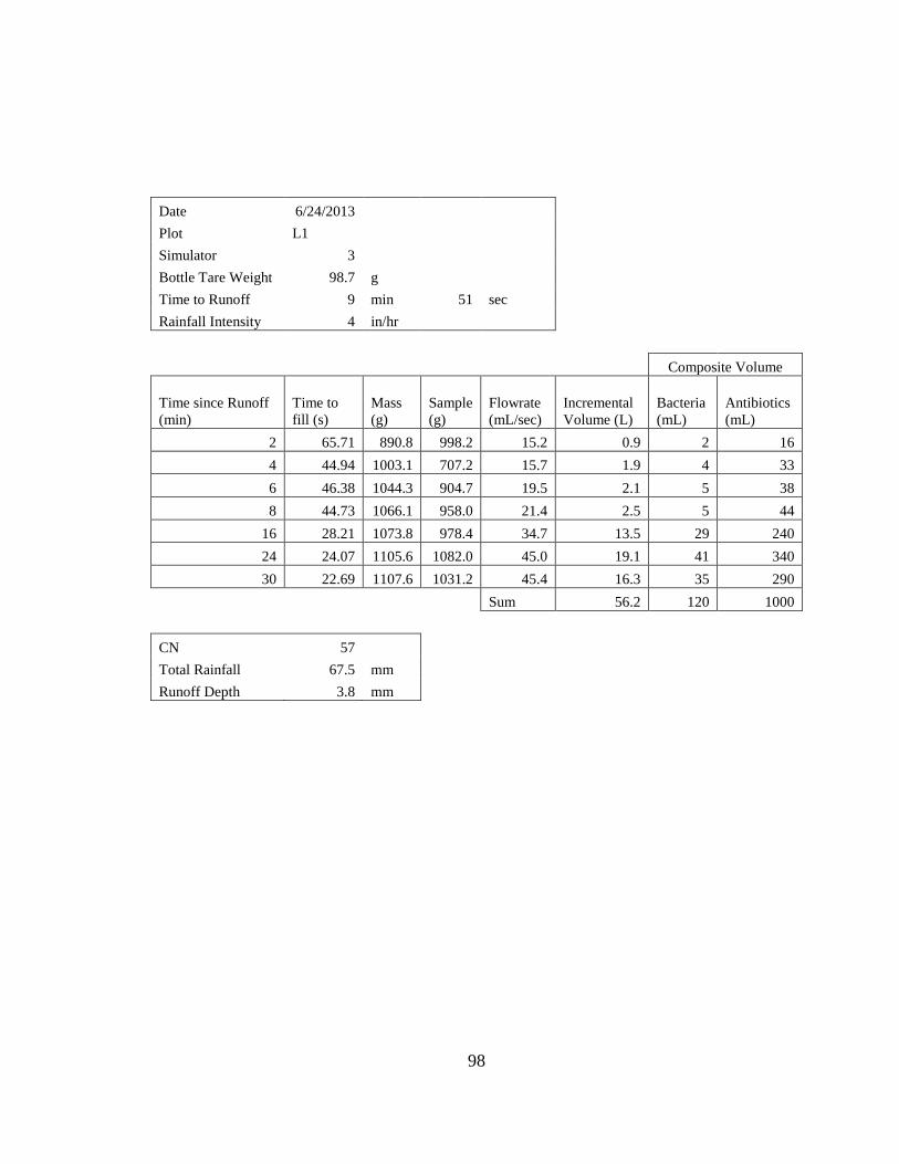
98

Date 6/24/2013

Plot L1

Simulator 3

Bottle Tare Weight 98.7 g



Composite Volume

Time since Runoff

(min)

Time to

fill (s)

Mass

(g)

Sample

(g)

Flowrate

(mL/sec)

Incremental

Volume (L)

Bacteria

(mL)

Antibiotics

(mL)

2 65.71 890.8 998.2 15.2 0.9 2 16

4 44.94 1003.1 707.2 15.7 1.9 4 33

6 46.38 1044.3 904.7 19.5 2.1 5 38

8 44.73 1066.1 958.0 21.4 2.5 5 44

16 28.21 1073.8 978.4 34.7 13.5 29 240

24 24.07 1105.6 1082.0 45.0 19.1 41 340

30 22.69 1107.6 1031.2 45.4 16.3 35 290

Sum 56.2 120 1000

CN 57


Runoff Depth 3.8 mm

99

Date 6/24/2013

Plot L3

Simulator 2

Bottle Tare Weight 98.7

Time to Runoff 27 min


Composite Volume

Time since Runoff

(min)

Time to

fill (s)

Mass

(g)

Sample

(g)

Flowrate

(mL/sec)

Incremental

Volume (L)

Bacteria

(mL)

Antibiotics

(mL)

2 45.32 962.4 863.7 19.1 1.1 3 27

4 39.47 966.2 867.5 22.0 2.5 7 58

6 40.49 990.2 891.5 22.0 2.6 7 62

8 38.48 1013.1 914.4 23.8 2.7 8 64

16 30.93 1011.5 912.8 29.5 12.8 36 299

24 39.48 950.9 852.2 21.6 12.3 34 287

30 30.86 932.2 833.5 27.0 8.7 25 204

Sum 42.8 120 1000

CN 44


Runoff Depth 2.9 mm

100

Date 6/24/2013

Plot N9

Simulator 4




Composite Volume

Time since Runoff

(min)

Time to

fill (s) Mass (g)

Sample

(g)

Flowrate

(mL/sec)

Incremental

Volume (L)

Bacteria

(mL)

Antibiotics

(mL)

2 60.80 575.3 476.6 7.8 0.5 4 23

4 61.65 609.9 511.2 8.3 1.0 7 47

6 59.66 681.0 582.3 9.8 1.1 8 52

8 55.66 706.0 607.3 10.9 1.2 10 60

16 101.59 931.7 833.0 8.2 4.6 35 222

24 92.98 862.4 763.7 8.2 3.9 30 191

30 90.31 972.3 873.6 9.7 3.2 25 156

Sum 15.5 120 750

CN 31


Runoff Depth 1.0 mm

101

Date 6/25/2013

Plot C3

Simulator 3



Composite Volume

Time since Runoff

(min)

Time to

fill (s)

Mass

(g)

Sample

(g)

Flowrate

(mL/sec)

Incremental

Volume (L)

Bacteria

(mL)

Antibiotics

(mL)

2 43.66 1072.6 973.9 22.3 1.3 3 23

4 35.24 1029.8 931.1 26.4 2.9 6 50

6 32.01 1023.5 924.8 28.9 3.3 7 57

8 29.35 1028.3 929.6 31.7 3.6 7 62

16 27.43 1005.7 907 33.1 15.5 32 265

24 22.21 1008.8 910.1 41.0 17.8 36 303

30 25.68 1068 969.3 37.7 14.2 29 241

Sum 58.7 120 1000

CN 38


Runoff Depth 3.9 mm

102

Date 6/25/2013

Plot C4

Simulator 3




Composite Volume

Time since Runoff

(min)

Time to

fill (s) Mass (g)

Sample

(g)

Flowrate

(mL/sec)

Incremental

Volume (L)

Bacteria

(mL)

Antibiotics

(mL)

2 55.36 674.5 575.8 10.4 0.6 10 62

4 54.83 574.1 475.4 8.7 1.1 18 113

6 53.97 416.1 317.4 5.9 0.9 14 86

8 220.54 823.8 725.1 3.3 0.6 9 54

16 224.74 814.1 715.4 3.2 1.6 25 154

24 171.66 754.1 655.4 3.8 1.7 27 166

30 210.74 653.3 554.6 2.6 1.2 18 115

Sum 7.6 120 750

CN 25


Runoff Depth 0.5 mm

103

Date 6/25/2013

Plot D5

Simulator 2




Composite Volume

Time since Runoff

(min)

Time to

fill (s)

Mass

(g)

Sample

(g)

Flowrate

(mL/sec)

Incremental

Volume (L)

Bacteria

(mL)

Antibiotics

(mL)

2 55.25 898.5 799.8 14.5 0.9 3 26

4 55.02 915.9 817.2 14.9 1.8 6 53

6 46.55 1037.2 938.5 20.2 2.1 8 63

8 55.13 732.7 634 11.5 1.9 7 57

16 37.18 1012.2 913.5 24.6 8.7 31 260

24 46.56 1010 911.3 19.6 10.6 38 318

30 45.21 1085.4 986.7 21.8 7.5 27 224

Sum 33.3 120 1000

CN 39


Runoff Depth 2.2 mm

104

Date 6/26/2013

Plot B1

Simulator 2




Composite Volume

Time since Runoff

(min)

Time to

fill (s)

Mass

(g)

Sample

(g)

Flowrate

(mL/sec)

Incremental

Volume Bacteria

(mL)

Antibiotics

(mL)

2 12.00 1004.8 906.1 75.5 4.5 2 15

4 9.34 1142.8 1044.1 111.8 11.2 5 38

6 6.81 1038.6 939.9 138.0 15.0 6 50

8 5.97 1067.4 968.7 162.3 18.0 7 60

16 5.18 1147.3 1048.6 202.4 87.5 35 292

24 4.99 1047.1 948.4 190.1 94.2 38 315

30 4.66 994.6 895.9 192.3 68.8 28 230

Sum 299.3 120 1000

CN 75


Runoff Depth 20.1 mm

105

Date 6/26/2013

Plot B4

Simulator 2




Composite Volume

Time since Runoff

(min)

Time to

fill (s)

Mass

(g)

Sample

(g)

Flowrate

(mL/sec)

Incremental

Volume (L)

Bacteria

(mL)

Antibiotics

(mL)

2 14.22 1042.1 943.4 66.3 4.0 3 22

4 11.55 1030.8 932.1 80.7 8.8 6 48

6 10.85 1088.5 989.8 91.2 10.3 7 56

8 9.05 1016.1 917.4 101.4 11.6 8 63

16 8.08 1075.6 976.9 120.9 53.3 35 290

24 8.11 1012.9 914.2 112.7 56.1 37 305

30 8.65 1044.0 945.3 109.3 40.0 26 217

Sum 184.1 120 1000

CN 69



106

Date 6/26/2013

Plot B10

Simulator 4




Composite Volume

Time since Runoff

(min)

Time to

fill (s) Mass (g)

Sample

(g)

Flowrate

(mL/sec)

Incremental

Volume (L)

Bacteria

(mL)

Antibiotics

(mL)

2 8.50 1020.1 921.4 108.4 6.5 3 27

4 6.71 990.9 892.2 133.0 14.5 7 59

6 6.36 1015.1 916.4 144.1 16.6 8 68

8 6.12 996.6 897.9 146.7 17.4 9 71

16 6.71 1096.2 997.5 148.7 70.9 35 290

24 6.76 1051.4 952.7 140.9 69.5 34 284

30 6.75 997.2 898.5 133.1 49.3 24 202

Sum 244.8 120 1000

CN 72



107

Date 6/26/2013

Plot C2

Simulator 3




Composite Volume

Time since Runoff

(min)

Time to

fill (s)

Mass

(g)

Sample

(g)

Flowrate

(mL/sec)

Incremental

Volume (L)

Bacteria

(mL)

Antibiotics

(mL)

2 38.19 1025.4 926.7 24.3 1.5 1 10

4 28.66 1076.2 977.5 34.1 3.5 3 24

6 22.28 1004.1 905.4 40.6 4.5 4 31

8 17.69 1096.3 997.6 56.4 5.8 5 40

16 10.09 1036.6 937.9 93.0 35.8 30 247

24 8.33 1059.4 960.7 115.3 50.0 41 345

30 7.39 1051.1 952.4 128.9 44.0 36 303

Sum 145.1 120 1000

CN 51


Runoff Depth 9.8 mm

108

Date 6/28/2013

Plot D1

Simulator 3




Composite Volume

Time since Runoff

(min)

Time to

fill (s)

Mass

(g)

Sample

(g)

Flowrate

(mL/sec)

Incremental

Volume (L)

Bacteria

(mL)

Antibiotics

(mL)

2 11.36 1065.7 967 85.1 5.1 1 12

4 5.95 1050.5 951.8 160.0 14.7 4 35

6 4.80 1103 1004.3 209.2 22.2 6 53

8 4.04 1039.7 941 232.9 26.5 8 63

16 3.54 1036.6 937.9 264.9 119.5 34 285

24 3.54 1129.9 1031.2 291.3 133.5 38 318

30 4.13 1143 1044.3 252.9 97.9 28 234

Sum 419.4 120 1000

CN 82



109

Date 7/2/2013

Plot C5

Simulator 2




Composite Volume

Time since Runoff

(min)

Time to

fill (s) Mass (g)

Sample

(g)

Flowrate

(mL/sec)

Incremental

Volume (L)

Bacteria

(mL)

Antibiotics

(mL)

2 6.97 1103.9 1005.2 144.2 8.7 3 28

4 5.27 1007.7 909.0 172.5 19.0 7 62

6 5.27 1037.2 938.5 178.1 21.0 8 69

8 5.30 1105.4 1006.7 189.9 22.1 9 72

16 5.47 1049.6 950.9 173.8 87.3 34 285

24 5.45 1019.7 921.0 169.0 82.3 32 269

30 4.87 1049.4 950.7 195.2 65.6 26 214

Sum 305.9 120 1000

CN 80



110

Date 7/2/2013

Plot B6

Simulator 4




Composite Volume

Time since Runoff

(min)

Time to

fill (s) Mass (g)

Sample

(g)

Flowrate

(mL/sec)

Incremental

Volume (L)

Bacteria

(mL)

Antibiotics

(mL)

2 9.08 1043.3 944.6 104.0 6.2 3 25

4 8.18 1048.6 949.9 116.1 13.2 6 53

6 7.64 1088.1 989.4 129.5 14.7 7 60

8 7.54 1094.7 996.0 132.1 15.7 8 64

16 6.41 1069.8 971.1 151.5 68.1 33 276

24 5.95 1012.9 914.2 153.6 73.2 36 297

30 6.47 1110.2 1011.5 156.3 55.8 27 226

Sum 247.0 120 1000

CN 76



111

Date 7/2/2013

Plot B5

Simulator 2




Composite Volume

Time since Runoff

(min)

Time to

fill (s) Mass (g)

Sample

(g)

Flowrate

(mL/sec)

Incremental

Volume (L)

Bacteria

(mL)

Antibiotics

(mL)

2 15.88 1037.6 938.9 59.1 3.5 2 13

4 9.24 1062.5 963.8 104.3 9.8 4 35

6 6.27 1066.7 968.0 154.4 15.5 7 55

8 5.68 1086.0 987.3 173.8 19.7 8 70

16 5.69 1132.9 1034.2 181.8 85.3 36 301

24 6.15 1119.7 1021.0 166.0 83.5 35 295

30 4.82 1057.8 959.1 199.0 65.7 28 232

Sum 283.1 120 1000

CN 80



112

Date 7/2/2013

Plot C6

Simulator 4



Rainfall Intensity 4

in/h

r

Composite Volume

Time since Runoff

(min)

Time to

fill (s)

Mass

(g)

Sample

(g)

Flowrate

(mL/sec)

Incremental

Volume(mL)

Bacteri

a (mL)

Antibiotic

s (mL)

2 53.02 569.2 470.5 8.9 0.5 3 27

4 53.92 659.2 560.5 10.4 1.2 7 58

6 54.53 699.3 600.6 11.0 1.3 8 64

8 55.02 733.5 634.8 11.5 1.4 8 68

16 76.41 1110.9 1012.2 13.2 5.9 36 297

24 72.4 1065.4 966.7 13.4 6.4 38 319

30 196.06 1118.0 1019.3 5.2 3.3 20 167

Sum 20.0 120 1000

CN 50


Runoff Depth 1.3 mm

113

APPENDIX C: METHODOLOGY FOR E.COLI ANALYSIS

114

Coliert-18, 120 mL IDEXX sample bottles (pre-sterilized) with sodium thiosulfate

(de-chlorinating agent), and Quanti-Tray*/2000 were purchase from IDEXX Laboratories

(Westbrook, ME). Dilutions (1:10, 1:100, and 1:1000) were made using sterilized

deionized water (DI H2O) and sterilized buffer water prepared by the following

instructions.

C.1 BUFFER WATER AND DI WATER PREPARATION

C.1.1 Prepare Solutions

1. Add 50g of MgSO4∙7H2O to 1 L flask of DI H2O.

2. Add 34g of KH2PO4 to a second 1 L flask of DI H2O and adjust pH to 7.2 with 1

N NaOH.

C.1.2 Prepare Buffer Water

3. Add 10 mL of MgSO4∙7H2O solution to a 2 L flask.

4. Add 2.5 mL of KH2PO4 solution to the same 2 L flask as in step 3.

5. Fill the remaining volume of the 2 L flask with DI H2O.

6. Securely place a lid on the 2 L flask. Mix the 2 L flask by inversion. Once mixing

is complete, loosen lid (e.g. enough to rattle), but such that it remains on the

threads.

C1.3 Prepare DI H2O

7. Fill a second 2 L flask with DI H2O. Place a lid on this 2 L flask. The lid should

be loose enough to rattle but still catch on threads.

C.1.4 Autoclave

8. Place autoclave tape on each lid (2 L flask of buffer water and 2 L flask of DI

H2O ) and check for proper looseness.

9. Autoclave on liquid cycle with the flasks in plastic trays.

10. Wait 10 minutes after cycle is complete before removing flasks.

11. Wait until the flasks are at room temperature before tightening the lids.

115

C.2 DILUTION BOTTLE PREPARATION

1. Place dilution bottles in plastic trays to prevent tipping. Lids should remain on

the sample bottles, but be loosened (e.g. still caught on the threads). Glass or

plastic 100-200 mL bottles are recommended.

2. Autoclave dilution bottles on labwares cycle.

3. Allow dilution bottles cool to room temperature before tightening lids.

C.3 DILUTIONS

1. Put 90 mL of buffer water into a sterilized dilution bottle (100-200 mL) to be used

for dilution series. When making three dilutions, as done in this study, two

sterilized dilution bottles with buffer are needed for each sample. See Figure C.1.

2. Put 90 mL of sterile DI H2O into the three sterilized dilution bottles to be used for

Coliert-18. One bottle for each dilution of each sample is needed for this step,

hence three dilutions require three bottles.

3. Add one packet of Coliert-18 to each sterilized dilution bottle containing DI H2O.

4. Add two drops of anti-foaming agent to each sterilized dilution bottle containing

DI H2O.

5. Put 10 mL of sample into 90 mL of DI H2O for the 1:10 Dilution. Empty all 100

mL into a Quanti-Tray.

6. Put 10 mL of sample into 90 mL of buffer water (dilution bottle prepared in step

1). This is the 1:10 buffer water and sample mixture.

7. Put 10 mL of the 1:10 buffer water and sample mixture (step 6) into 90 mL of DI

H2O and empty all 100 mL into a Quanti-Tray. This is the 1:100 dilution.

8. Add 10 mL of the 1:10 buffer water and sample mixture (step 6) to 90 mL of

buffer water. This is the 1:100 buffer water.

9. Put 10 mL of the 1:100 buffer water and sample mixture (step 8) in 90 mL of DI

H2O for the 1:1000 dilution and empty all 100 mL into a Quanti-Tray.

10. Continue this process for each subsequent dilution needed.

After emptying each dilution into its respective tray, seal using the IDEXX sealer. Place

the sealed tray in an incubator for 18-22 hours at 35°C±0.5°C. After the incubation

116

period, use a UV-light to determine which cells tested positive for E. coli. Cells must

turn yellow and fluoresce to be considered positive. If unsure, use the IDEXX

comparator tray to compare samples to the standard.

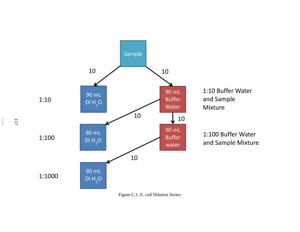
117

Figure C.1. E. coli Dilution Series.

Sample

90 mL DI H

2O

90 mL Buffer water

90 mL DI H

2O

90 mL Buffer Water

90 mL

DI H2O

10 mL

10 mL

10 mL

10 mL

10 mL

1:10 Dilution

1:100 Dilution

1:1000 Dilution

1:10 Buffer Water and Sample Mixture

1:100 Buffer Water and Sample Mixture

118

APPENDIX D: METHODOLOGY FOR ANTIBIOTIC EXTRACTION AND

ANALYSIS

119

The first step in antibiotic analysis is sample concentration. This step is necessary

due to the low concentrations (mg) typicaly found in water samples. Typically, this

concentration step is performed via solid phase extraction. However, the method of solid

phase extraction is quite time consuming and often results in low recovery rates of

antibiotics (Yang et al., 2005; Zhu et al,. 2001). As such, a new methodology was

developed whereby the process of lyophilization (freeze-drying), similar to that described

by Hirsh et al. (1998), was used.

D.1 SAMPLE PREPARATION

Approximately, 50 mL of sample was added to a 50 mL centrifuge tube. The

sample, in the centrifuge tube, was then centrifuged at 3,500 rpm for 20 minutes. Next,

45 mL of supernatant was pipetted into a 50 mL glass test tube. The test tube was then

covered with a kimwipe that was secured in place with tape. Note that filtering sample

through a 0.45 µm filter prior to its placement in a glass test tube would likely help refine

the chromatogram.

D.2 LYOPHILIZATION

Samples were placed in a freezer (-4°C) for 12 hours prior to placement in a

-40°C freezer for about 2 hours to further lower the temperature. An SP Scientific VirTis

Wizard 2.0 lyophilzer (Gardiner, New York) was turned on to the freeze cycle until the

shelf temperature reached approximately -20°C. Samples were then removed from the -

40°C freezer and placed in the lyophilizer. Note that while samples can be frozen in the

lyophilzer, a greater potential exists for the test tubes to break due to the rapidness of

freezing; hence the reason for using the freezer.

The lyophilizer condenser was turned on and allowed to reach a temperature between -

40°C and -60°C. The lyophilizer vacuum was turned on and allowed to reach less than

500 mTorr. Shelf control for the lyophilizer was turned on and began heating the shelf to

10°C. Samples were left in the lyophilizer until dry (approximately 3 days).

D.3 SAMPLE CONCENTRATION

Dry residue in the test tubes was re-dissolved in 900 µL of 50% methanol solution

by rinsing the test tube with 300 µL of methanol three times. The solution was then

120

transferred to micro-centrifuge tubes and centrifuged at 4,000 rpm for 10 minutes.

Approximately, 600 µL of supernatant was then transferred to HPLC vials.

A solution containing an oxytetratcycline concentration of 2 µg mL-1

was made

by diluting a 1 mg mL-1

oxytetracycline solution. A 300 µL glass insert was then placed

in an HPLC vial and 100 µL of concentrated sample was added to 100 µL of the 2 µg

mL-1

solution. This resulted in a 25X concentration from the original sample and a

concentration of at least 1 µg L-1

of oxytetracycline.

D.4 HPLC

A Dionex Ultimate 3000 HPLC along with an Ultimate 3000RS Variable

Wavelength detector (Sunnyvale, California) set was used for this analysis. The variable

wavelength detector was set at a wave length of 290 nm (Kay et al., 2005). A Dionex

Acclaim 120 (C18) column with an inner diameter of 3 µm and length of 250 mm was

used. The pumping rate was set to 0.400 mL min-1

with a gradient mobile phase of 0.5%

acetic acid in water and 0.5% acetic acid in methanol. The gradient can be seen in Table

D.1. The HPLC injected 20 µL of 25X concentrated sample and ran for 12 minutes per

sample.

Table D.1. HPLC Gradient used in Oxytetracycline Analysis.

Time (min) HPLC Gradients

1

A (%) B (%)

1 60 40

4 10 90

7 10 90

9 40 60

10 60 40 1A is DI water with 0.5% acetic acid; B is HPLC grade MeOH with 0.5% acetic acid.

121

APPENDIX E: MANURE AND SOIL SAMPLING RESULTS

122

Table E.1. Results of Manure Analysis.

Plot1 C (%) N (%) P (%) K (%) Ca (%) Mg (%) Zn (mg L

-1) Cu (mg L

-1) Mn (mg L

-1) Fe (mg L

-1)

-----------------------M-----------------------

B4 1.99 0.49 0.09 0.24 0.11 0.04 34.62 3.46 13.85 103.86

C5 1.95 0.49 0.09 0.23 0.12 0.04 37.80 3.78 15.12 98.28

L1 1.99 0.49 0.08 0.25 0.11 0.03 35.71 3.57 14.28 85.70

-----------------------MA------------------------

B6 1.72 0.45 0.08 0.25 0.13 0.04 60.67 3.79 15.17 75.84

B10 2.03 0.49 0.09 0.25 0.11 0.04 39.08 3.55 14.21 95.94

C3 2.10 0.49 0.09 0.25 0.11 0.04 36.78 3.68 14.71 114.00

L3 2.06 0.49 0.08 0.25 0.11 0.04 37.07 3.71 14.83 70.43

-----------------------MAA------------------------

B1 2.07 0.50 0.09 0.29 0.12 0.04 47.01 7.23 14.46 86.78

B5 2.17 0.53 0.10 0.30 0.12 0.04 52.75 12.17 16.23 93.33

C4 1.79 0.48 0.09 0.27 0.12 0.04 44.14 8.03 16.05 112.36

N9 1.94 0.52 0.10 0.30 0.11 0.04 49.04 12.26 16.35 93.98 1M=manure only, MA=manure and antibiotics, MAA=manure, antibiotics, and alum.

123

Table E.2. Results of Soil Analysis.

Plot1

P (lb

ac-1

)

K (lb

ac-1

) pH

Ca

(lb

ac-1

)

Mg

(lb

ac-1

)

Zn

(lb

ac-1

)

Total

N

(%)

Total

C

(%)

Sand

(%)

Silt

(%)

Clay

(%)

Moisture

(%)

-----------------------C-----------------------

C2 160 439 5.08 4,147 326 7.8 0.18 1.63 10.04 70.11 19.85 22.6

C6 169 520 4.95 2,989 338 10.8 0.20 1.79 10.01 72.96 17.03 29.9

D1 269 554 5.91 4,895 548 7.8 0.18 1.51 9.91 74.28 15.81 24.2

D5 164 384 5.17 3,913 298 9.0 0.17 1.64 12.14 62.75 25.11 23.8

-----------------------M-----------------------

B4 233 484 5.03 2,517 597 10.7 0.22 2.03 11.75 73.18 15.07 32.6

C5 184 584 5.28 3,755 317 35.6 0.21 2.00 13.21 69.33 17.46 29.8

L1 282 542 5.26 3,181 699 5.6 0.20 1.77 9.67 73.57 16.76 29.5

-----------------------MA-----------------------

B6 194 901 5.09 3,024 377 8.7 0.25 2.15 10.82 72.31 16.87 30.6

B10 149 587 5.25 3,297 832 5.0 0.20 1.80 10.37 70.41 19.21 30.3

C3 258 419 5.57 3,809 822 13.8 0.24 2.25 11.01 74.94 14.05 29.1

L3 234 519 5.32 3,540 850 6.4 0.20 1.89 14.25 62.01 23.71 30.0

-----------------------MAA-----------------------

B1 200 506 5.39 2,958 596 8.0 0.20 1.91 10.67 74.60 14.73 31.3

B5 175 601 5.1 3,427 421 23.6 0.21 1.90 11.67 70.76 17.57 29.0

C4 353 850 5.66 4,579 810 25.8 0.30 3.12 13.75 70.44 15.81 29.5

N9 137 264 5.28 2,972 729 4.2 0.17 1.48 7.95 75.16 16.88 29.0 1M=manure only, MA=manure and antibiotics, MAA=manure, antibiotics, and alum.

124

REFERENCES

[ACAAI] American College of Allergy, Asthma, and Immunology. 2013. Penicillin

Allergy. Available at: http://www.acaai.org/allergist/allergies/Types/drug-

allergy/Pages/penicillin-allergy.aspx. Accessed on December 16, 2013.

Adams, C., Y. Wang, K. Loftin, and M. Meyer. 2002. Removal of Antibiotics from

Surface and Distilled Water in Conventional Water Treatment Processes. Journal

of Environmental Engineering 128(3): 253-260.

Agouridis, C.T., and D.R. Edwards. 2003. The Development of Relationships between

Constituent Concentrations and Generic Hydrological Variables. Transactions of

the ASAE 46(2): 245-256.

Alexander, R.B., R.A. Smith, G.E. Schwarz, E.W. Boyer, J.V Nolan, and J.W. Brakebill.

2007. Differences in Phosphorus and Nitrogen Delivery to the Gulf of Mexico

from the Mississippi River Basin. Environmental Science and Technology 42(3):

822-830.

[APHA] American Public Health Association. 1998. Standard Methods for the

Examination of Water and Wastewater, 20th

edition. Clesceri, L.S., A.E.

Greenberg, and A.D. Eaton (eds.). American Public Health Association,

Baltimore, MD.

Arikan, O.A., C. Rice, E. Codling. 2008. Occurrence of Antibiotics and Hormones in a

Major Agricultural Watershed. Desalination 226(1): 121-133.

Arikan, O.A., L.J. Sikora, W. Mulbry, S.U. Khan, and G.D. Foster. 2007. Composting

Rapidly Reduces Levels of Extractable Oxytetracycline in Manure from

Therapeutically Treated Beef Calves. Bioresource Technology 98(1): 169-176.

Aulenbach, B.T. and R.P. Hooper. 2006. The Composite Method: an Improved Method

for Stream‐water Solute Load Estimation. Hydrological Processes 20(14): 3029-

3047.

Baguer, A.J., J. Jensen, and P.H. Krogh. 2000. Effects of the Antibiotics

Oxytetracycline and Tylosin on Soil Fauna. Chemosphere 40(7): 751-757.

Brady, N.C. and R.R. Weil. 1996. The Nature and Properties of Soils, 11th

ed. Prentice-

Hall Inc., Upper Saddle River, NJ.

125

Braskerud, B.C. 2002. Factors affecting Phosphorus Retention in Small Constructed

Wetlands Treating Agricultural Non-point Source Pollution. Ecological

Engineering 19(1): 41-61.

Brorsen, B.W., T. Lehenbauer, D. Ji, and J. Connor. 2002. Economic Impacts of

Banning Subtherapeutic Use of Antibiotics in Swine Production. Journal of

Agricultural and Applied Economics 34(3): 489-500.

Bulson, P.C., D.L. Johnstone, H.L. Gibbons, and W.H. Funk, W. H. 1984. Removal and

Inactivation of Bacteria during Alum Treatment of a Lake. Applied and

Environmental Microbiology 48(2): 425-430.

Burkhardt, M., C. Stamm, C. Waul, H. Singer, and S. Müller. 2005. Surface Runoff and

Transport of Sulfonamide Antibiotics and Tracers on Manured

Grassland. Journal of Environmental Quality 34(4): 1363-1371.

Bushee, E.L., D.R. Edwards, and P.A. Moore. 1998. Quality of Runoff from Plots

Treated with Municipal Sludge and Horse Bedding. Transactions of the

ASAE 41(4): 1035-1041.

Bushee-Bullock, E. L. 1999. Effects of Chemical Amendments on Gaseous Emissions

and Surface Water Runoff Concentration from Swine Manure. Master’s Thesis,

University of Kentucky, Lexington, KY.

Campagnolo, E.R., K.R Johnson, A. Karpati, C.S. Rubin, D.W. Kolpin, M.T, Meyer, E.J.

Esteban, R.W. Currier, K. Smith, K.M. Thu, and M. McGeehin. 2002.

Antimicrobial Residues in Animal Waste and Water Resources Proximal to

Large-scale Swine and Poultry Feeding Operations. Science of the Total

Environment 299(1): 89-95.

[NSTC-CENR] National Science and Technology Council Committee on Environment

and Natural Resources. 2000. Integrated Assessment of Hypoxia in the Northern

Gulf of Mexico. National Science and Technology Council Committee on

Environment and Natural Resources, Washington, DC, USA. Available at:

http://oceanservice.noaa.gov/products/hypox_final.pdf. Accessed on December 1,

2013.

126

Chee-Sanford, J.C., R. I. Aminov, I. J. Krapac, N. Garrigues-Jeanjean, and R.I. Mackie.

2001. Occurrence and Diversity of Tetracycline Resistance Genes in Lagoons

and Groundwater Underlying Two Swine Production Facilities. Applied and

Environmental Microbiology 67(4): 1494-1502.

Chee-Sanford, J.C., R.I. Mackie, S. Koike, I.G. Krapac, Y.. Lin, A.C. Yannarell, S.

Maxwell, and R.I. Aminov. 2009. Fate and Transport of Antibiotic Residues and

Antibiotic Resistance Genes Following Land Application of Manure

Waste. Journal of Environmental Quality 38(3): 1086-1108.

Cooke, G.D., E. B. Welch, S. A. Peterson, and P. R. Newroth. 1986. Lake and Reservoir

Restoration. Butterworth Publishers, Stoneham, MA

Cooke, S.E., S.M. Ahmed, N. MacAlpine. 2000. Introductory Guide to Surface Water

Quality Monitoring in Agriculture. Conservation and Development Branch,

Alberta Agriculture, Food and Rural Development. Available at:

http://www1.agric.gov.ab.ca/$department/deptdocs.nsf/all/wat2417. Accessed

October 15, 2013.

Davis, J.G., C.C. Truman, S.C. Kim, J.C. Ascough, and K. Carlson. 2006. Antibiotic

Ttransport via Runoff and Soil Loss. Journal of Environmental Quality 35(6):

2250-2260.

DeLaune, P.B. and P.A. Moore Jr. 2013. 17β-estradiol in Runoff as Affected by Various

Poultry Litter Application Strategies. Science of the Total Environment 444: 26-

31.

Delpla, I., E. Baurès, A.V. Jung, O. Thomas. 2011. Impacts of Rainfall Events on

Runoff Water Quality in an Agricultural Environment in Temperate Areas.

Science of the Total Environment 409(9): 1683-1688.

Dewey, C.E., B.D. Cox, B.E. Straw, E. J. Bush, and H.S. Hurd. 1997. Associations

between Off-label Feed Additives and Farm size, Veterinary Consultant Use, and

Animal Age. Preventive Veterinary Medicine 31(1): 133-146.

Doi, A.M. and M.K. Stoskopf. 2000. The Kinetics of Oxytetracycline Degradation in

Deionized Water under Varying Temperature, pH, Light, Substrate, and Organic

Matter. Journal of Aquatic Animal Health 12(3): 246-253.

127

Dolliver, H.A., and S.C. Gupta. 2008a. Antibiotic Losses in Leaching and Surface

Runoff from Manure-amended Agricultural Land. Journal of Environmental

Quality 37(3): 1227-1237.

Dolliver, H. A. and S. Gupta, S.C. 2008b. Antibiotic Losses from Unprotected Manure

Stockpiles. Journal of Environmental Quality 37(3): 1238-1244.

Durhan, E.J., C.S. Lambright, E.A. Makynen, J. Lazorchak, P.C. Hartig, V.S. Wilson,

and G.T. Ankley. 2006. Identification of Metabolites of Trenbolone Acetate in

Androgenic Runoff from a Beef Feedlot. Environmental Health

Perspectives 114(S-1): 65.

Edwards, D.R. and T.C. Daniel. 1992. Potential Runoff Quality Effects of Poultry

Manure Slurry Applied to Fescue Plots. Transactions of the ASAE 35(6): 1827-

1832.

Edwards, D.R., P.A. Moore, S.R. Workman, E.L. Bushee. 1999. Runoff of Metals from

Alum-Treated Horse Manure and Municipal Sludge. Journal of the American

Water Resources Association 35(1): 155-165.

Edwards, D.R., T.K. Hutchens, R.W. Rhodes, B.T. Larson, and L. Dunn. 2000. Quality

of Runoff from Plots with Simulated Grazing. Journal of the American Water

Resources Association 36(5): 1063-1073.

Eghball, B. and J.F. Power. 1999. Composted and Noncomposted Manure Application

to Conventional and No-tillage Systems: Corn Yield and Nitrogen

Uptake. Agronomy Journal 91(5): 819-825.

Gerba, C.P. and J.E. Smith. 2005. Sources of Pathogenic Microorganisms and Their

Fate During Land Application of Wastes. Journal of Environmental

Quality 34(1): 42-48.

Halling-Sørensen, B. 2000. Algal Toxicity of Antibacterial Agents Used in Intensive

Farming. Chemosphere 40(7): 731-739

Harmel, R.D. and K.W. King. 2005. Uncertainty in Measured Sediment and Nutrient

Flux in Runoff from Small Agricultural Watersheds. Transactions of the

ASAE 48(5): 1713-1721.

128

Harmel, R.D., R.J. Cooper, R.W. Slade, R.L. Haney, and J.G. Arnold. 2006. Cumulative

Uncertainty in Measured Streamflow and Water Quality Data for Small

Watersheds. Transactions of the ASAE 49(3): 689-701.

Higgins, S., A. Gumbert, and S. Mehlhope. 2013. ID-211 Kentucky nutrient

management planning guide. University of Kentucky Cooperative Extension

Service.

Hirsch, R., T.A. Ternes, K. Haberer, A. Mehlich, F. Ballwanz, F., and K.L. Kratz. 1998.

Determination of Antibiotics in Different Water Compartments via Liquid

Chromatography–electrospray Tandem Mass Spectrometry. Journal of

Chromatography A 815(2): 213-223.

Hirsch, R., T. Ternes, K. Haberer, and K.L. Kratz. 1999. Occurrence of Antibiotics in

the Aquatic Environment. Science of the Total Environment 225(1): 109-118.

Hoos, A.B., J.A. Robinson, R.A. Aycock, R.R. Knight, and M.D. Woodside. 2000.

Sources, Instream Transport, and Trends of Nitrogen, Phosphorus, and Sediment

in the Lower Tennessee River Basin, 1980-96. US Department of the Interior, US

Geological Survey.

Huang, G.F., Q.T. Wu, J.W.C. Wong, and B.B. Nagar. 2006. Transformation of Organic

Matter during Co-composting of Pig Manure with Sawdust. Bioresource

Technology 97(15): 1834-1842.

Huber, D.R. 1993. Contaminant Transport in Surface Water. Chapter 14 in Handbook

of Hydrology. D.R. Maidment (ed.). New York, N.Y.: McGraw-Hill.

Jalonick, M.C. 2013. FDA Takes Steps to Phase Out Antibiotics in Meat. Lexington

Herald Leader. December 11, 2013. Available at:

http://www.kentucky.com/2013/12/11/2982600/fda-targets-antibiotics-in-

meat.html. Accessed on December 19, 2013.

Kato, T., H. Kuroda, and H. Nakasone. 2009. Runoff Characteristics of Nutrients from

an Agricultural Watershed with Intensive Livestock Production. Journal of

Hydrology 368(1): 79-87.

Kay, P., P.A. Blackwell, and A. Boxall. 2005. Transport of Veterinary Antibiotics in

Overland Flow Following the Application of Slurry to Arable Land.

Chemosphere 59(7): 951-959.

129

[KDOW] Kentucky Division of Water. 2010. 2010 Integrated Water Quality Report:

Executive Summary. Available at: http://water.ky.gov/waterquality/Integrated

Reports/ExecutiveSummary2010.pdf. Accessed on December 13, 2013.

Kemper, N. 2008. Veterinary Antibiotics in the Aquatic and Terrestrial

Environment. Ecological Indicators 8(1): 1-13.

Khaleel, R., K.R. Reddy, and M.R. Overcash. 1980. Transport of Potential Pollutants in

Runoff Water from Land Areas Receiving Animal Wastes: a Review. Water

Research 14(5): 421-436.

Kim, S.C., J.G. Davis, C.C. Truman, J.C. Ascough II, and K. Carlson. 2010. Simulated

Rainfall Study for Transport of Veterinary Antibiotics–Mass Balance

Analysis. Journal of Hazardous Materials 175(1): 836-843.

Kolpin, D., E. Furlong, M. Meyer, E.M. Thurman, S. Zaugg, L. Barber, and H. Buxton.

2002. Pharmaceuticals, Hormones, and Other Organic Wastewater Contaminants

in U.S. Streams, 1999-2000: A National Reconnaissance USGS Staff -- Published

Research Paper 68. Available at: http://digitalcommons.unl.edu/usgsstaffpub/68.

Accessed on December 1, 2013.

Krapac, I.G., W.S. Dey, W.R. Roy, C.A. Smyth, E. Storment, S.L. Sargent, and J.D.

Steele. 2002. Impacts of Swine Manure Pits on Groundwater Quality.

Environmental Pollution 120(2): 475-492.

Kreuzig, R., S. Höltge, J. Brunotte, N. Berenzen, J. Wogram, and R. Schulz. 2005. Test‐

plot Studies on Runoff of Sulfonamides from Manured Soils after Sprinkler

Irrigation. Environmental Toxicology and Chemistry 24(4): 777-781.

Kulshrestha, P., R.F. Giese, D.S. Aga. 2004. Investigating the Molecular Interactions of

Oxytetracycline in Clay and Organic Matter: Insights on Factors Affecting its

Mobility in Soil. Environmental Science and Technology 38(15): 4097-4105.

Kumar, K.C., S. Gupta, Y. Chander, and A.K. Singh. 2005. Antibiotic Use in

Agriculture and Its Impact on the Terrestrial Environment. Advances in

Agronomy 87: 1-54.

Kümmerer, K. 2003. Significance of Antibiotics in the Environment. Journal of

Antimicrobial Chemotherapy 52(1): 5-7.

130

LaShore, S. and A. Pruden. (Eds.). 2009. Hormones and Pharmaceuticals Generated by

Concentrated Animal Feeding Operations (Vol. 1). Springer, New York, NY.

Lee, L.S., N. Carmosini, S.A. Sassman, H.M. Dion, and M.S. Sepulveda. 2007.

Agricultural Contributions of Antimicrobials and Hormones on Soil and Water

Quality. Advances in Agronomy 93: 1-68.

Lin, C.H., R.N. Lerch, K.W. Goyne, and H.E. Garrett. 2011. Reducing Herbicides and

Veterinary Antibiotics Losses from Agroecosystems Using Vegetative

Buffers. Journal of Environmental Quality 40(3): 791-799.

Lindsey, M.E., M. Meyer, E.M. Thurman. 2001. Analysis of Trace Levels of

Sulfonamide and Tetracycline Antimicrobials in Groundwater and Surface Water

using Solid-Phase Extraction and Liquid Chromatography/Mass Spectrometry.

Analytical Chemistry 73(19): 4640-4646.

Loke, M.L., J. Tjørnelund, B. Halling-Sørensen. 2002. Determination of the Distribution

Coefficient (log Kd) of Oxytetracycline, Tylosin A, Olaquindox and

Metronidazole in Manure. Chemosphere 48(3): 351-361.

Mason, L.B., C. Amrhein, C.C. Goodson, M.R. Matsumoto, and M. A. Anderson. 2005.

Reducing Sediment and Phosphorus in Tributary Waters with Alum and

Polyacrylamide. Journal of Environmental Quality 34(6): 1998-2004.

Mawdsley, J.L., R.D. Bardgett, R.J. Merry, B.F. Pain, and M.K. Theodorou. 1995.

Pathogens in Livestock Waste, Their Potential for Movement through Soil and

Environmental Pollution. Applied Soil Ecology 2(1): 1-15.

McEwen, S.A. and P.J. Fedorka-Cray. 2002. Antimicrobial Use and Resistance in

Animals. Clinical Infectious Diseases 34(Supplement 3): S93-S106.

McKeon, D.M., J.P. Calabrese, and G.K. Bissonnette. 1995. Antibiotic Resistant Gram-

Negative Bacteria in Rural Groundwater Supplies. Water Research 29(8): 1902-

1908.

Miller, W.P. 1987. A Solenoid-Operated, Variable Intensity Rainfall Simulator. Soil

Science Society of America Journal 51(3): 832-834.

Moore, P.A. and D.M. Miller. 1994. Decreasing Phosphorus Solubility in Poultry Litter

with Aluminum, Calcium, and Iron Amendments. Journal of Environmental

Quality 23(2): 325-330.

131

Moore, P.A., T.C.Daniel, J.T. Gilmour, B.R. Shreve, D.R. Edwards, and B.H. Wood.

1998. Decreasing Metal Runoff from Poultry Litter with Aluminum

sulfate. Journal of Environmental Quality 27(1): 92-99.

Mueller, D.K. and J.D. Stoner. 1998. Identifying the Potential for Nitrate Contamination

of Streams in Agricultural Areas of the United States. U.S. Geological Survey,

National Water–Quality Monitoring Council, Reston, VA.

[NLM] National Library of Medicine. 2005. Terramycin (Oxytetracycline

Hydrochloride) Capsule. Available at:

http://dailymed.nlm.nih.gov/dailymed/lookup.cfm? setid=6b4de8c9-8a32-4a07-

9183-419d6177ea08. Accessed on October 16, 2013.

[NRCS] Natural Resource Conservation Service. 2012. Conservation Practice Standard

Nutrient Management (Code 590). Available at: ftp://ftp-

fc.sc.egov.usda.gov/NHQ/practice-standards/standards/590.pdf/ Accessed

December 1, 2013.

[NRCS] Natural Resource Conservation Service. 2013. United States Department of

Agriculture. Web Soil Survey 3.0. Available at:

http://websoilsurvey.nrcs.usda.gov/. Accessed November 27, 2013.

Penn, C.J. and R.B. Bryant. 2006. Application of Phosphorus Sorbing Materials to

Streamside Cattle Loafing Areas. Journal of Soil and Water Conservation 61(5):

303-310.

Punamiya, P., D. Sarkar, S. Rakshit, and R. Datta. 2013. Effectiveness of Aluminum-

based Drinking Water Treatment Residuals as a Novel Sorbent to Remove

Tetracyclines from Aqueous Medium. Journal of Environmental Quality 42(5):

1449-1459.

Rickert, D.A. 1985. Water Quality—Compensation for Discharge in Detecting Trends in

Water Quality Data. Quality of Water Branch Memorandum No. 85.17. U.S.

Geological Survey, Reston, VA.

Sansalone, J.J. and S.G. Buchberger. 1997. Partitioning and First Flush of Metals in

Urban Roadway Storm Water. Journal of Environmental Engineering 123(2):

134-143.

132

Sarmah, A.K., M.T. Meyer, and A. Boxall. 2006. A Global Perspective on the Use,

Sales, Exposure Pathways, Occurrence, Fate and Effects of Veterinary Antibiotics

(VAs) in the Environment. Chemosphere 65(5): 725-759.

SAS Institute Inc. 2013. SAS/STAT® 13.1 User’s Guide. SAS Institute Inc., Cary, NC.

Sharpley, A. and P. Kleinman. 2003. Effect of Rainfall Simulator and Plot Scale on

Overland Flow and Phosphorus Transport. Journal of Environmental Quality

32(6): 2172-2179.

Smith, D. R., Moore, P. A., Griffis, C. L., Daniel, T. C., Edwards, D. R., & Boothe, D. L.

2001. Effects of alum and aluminum chloride on phosphorus runoff from swine

manure. Journal of Environmental Quality, 30(3), 992-998.

Soupir, M.L., S.S. Mostaghimi, E.R. Yagow, C.C. Hagedorn, and D.H. Vaughan. 2006.

Transport Of Fecal Bacteria From Poultry Litter and Cattle Manures Applied to

Pastureland. Water, Air and Soil Pollution 169(1-4): 125-136.

Stackelberg, P.E., J/ Gibs, E.T. Furlong, M.T. Meyer, S.D. Zaugg, and R.L. Lippincott.

2007. Efficiency of Conventional Drinking-Water-Treatment Processes in

Removal of Pharmaceuticals and Other Organic Compounds. Science of the

Total Environment 377(2): 255-272.

Stone, K.C., P.G. Hunt, J.M. Novak, M.H. Johnson, D.W. Watts. 2000. Flow-

Proportional, Time-Composited, and Grab Sample Estimation of Nitrogen Export

from an Eastern Coastal Plain Watershed. Transactions of the ASAE 43(2): 281-

290.

Tchobanoglous, G., F.L. Burton, and H.D. Stensel. 2002. Wastewater Engineering:

Treatment and Reuse. 4th

ed. McGraw-Hill, New York, New York.

Thuy, P.T., K. Moons, J.C. Van Dijk, N. Viet Anh, and B. Van der Bruggen. 2008. To

What Extent are Pesticides Removed from Surface Water During Coagulation–

Flocculation? Water and Environment Journal 22(3): 217-223.

Tolls, J. 2001. Sorption of Veterinary Pharmaceuticals in Soils: a Review.

Environmental Science and Technology 35(17): 3397-3406.

[UK] University of Kentucky Cooperative Extension Service. 2012. AGR-1: 2012-2013

Lime and Nutrient Recommendations.

133

[USDA] United States Department of Agriculture. 1996. Animal and Plant Health

Inspection Service. Veterinary Services, National Animal Health Monitoring

System (US). Antibiotic Usage in Premarket Swine. APHIS Veterinary Services

Factsheet, January 1996, Fort Collins, CO. Centres for Epidemiology and Animal

Health, USDA:APHIS:VS

[USDA] United States Department of Agriculture. 2001. Part I: Reference of Swine

Health and Management in the United States, 2000, National Animal Health

Monitoring System. Fort Collins, CO. #N338.0801.

[USDA] United States Department of Agriculture. 2009. 2007 Census of agriculture. AC-

07-A-51. Volume 1. USDA, National Agricultural Statistics Service. Geographic

Area Series, Washington, DC. Available at:

http://www.agcensus.usda.gov/Publications/2007/Full_Report/usv1.pdf. Accessed

October 15, 2013.

[USEPA] United States Environmental Protection Agency. 1973. Methods for

Identifying and Evaluating the Nature and Extent of Nonpoint Sources of

Pollutants. Paper No.430/9–73–014. Washington, D.C.: U.S. Environmental

Protection Agency, Office of Air and Water Programs.

[USEPA] United States Environmental Protection Agency Hazardous Waste

Management Division. 1991. Chemical Concentration Data Near the Detection

Limit (903891001). Available at:

http://nepis.epa.gov/Exe/ZyPURL.cgi?Dockey=9100S9OP.txt. Accessed on

November 27, 2013.

[USEPA] United States Environmental Protection Agency. Environmental Monitoring

and Support Laboratory Cincinnati. 1982. Handbook for Sampling and Sample

Preservation of Water and Wastewater (Vol. 83, No. 124503).

[USEPA] United States Environmental Protection Agency. 2013. Literature Review of

Contaminants in Livestock and Poultry Manure and Implications for Water

Quality (EPA 820-R-13-002)

Veni, G. 2002. Revising the Karst Map of the United States. Journal of Cave and Karst

Studies 64(1): 45-50.

134

Xuan, R., L. Arisi, Q. Wang, S.R. Yates, and K.C. Biswas. 2009. Hydrolysis and

Photolysis of Oxytetracycline in Aqueous Solution. Journal of Environmental

Science and Health Part B 45(1): 73-81.

Yang, S., J. Cha, K. Carlson. 2005. Simultaneous Extraction and Analysis of 11

Tetracycline and Sulfonamide Antibiotics in Influent and Effluent Domestic

Wastewater by Solid-Phase Extraction and Liquid Chromatography-Electrospray

Ionization Tandem Mass Spectrometry. Journal of Chromatography A 1097(1):

40-53.

Ye, Z., H.S. Weinberg, and M.T. Meyer. 2007. Trace Analysis of Trimethoprim and

Sulfonamide, Macrolide, Quinolone, and Tetracycline Antibiotics in Chlorinated

Drinking Water Using Liquid Chromatography Electrospray Tandem Mass

Spectrometry. Analytical Chemistry 79(3): 1135-1144.

Zar, J.H. 1999. Biostatistical Analysis, 4th

ed. Prentice Hall, New York, NY.

135

VITA

PLACE OF BIRTH

Elizabethtown, Kentucky

EDUCATION

B.S. Biosystems and Agricultural Engineering, University of Kentucky, Lexington,

Kentucky,

May 2012

Graduate Certificate, Stream and Watershed Science, University of Kentucky, Lexington,

Kentucky, May 2013

PROFESSIONAL EXPERIENCE

Graduate Research Assistant, Department of Biosystems and Agricultural Engineering,

University of Kentucky, Lexington, Kentucky. May 2012 – January 2014. Advisor: Dr.

C. T. Agouridis.

Teaching Assistant, Department of Biosystems and Agricultural Engineering,

University of Kentucky, Lexington, Kentucky. January 2013-May 2013

LICENSURE AND CERTIFICATION

Engineer-in-Training, Commonwealth of Kentucky, (Certificate No. 14460) September 21, 2012

PROFESSIONAL SOCIETIES

American Society of Agricultural and Biological Engineers

Society of Women Engineers

EVALUATING SAMPLING STRATEGIES FOR RAINFALL …

Documents

Transcript of EVALUATING SAMPLING STRATEGIES FOR RAINFALL …