Evaluating rainwater harvesting on watershed level in the ...
113
Faculty of Bioscience Engineering Academic year 2010 – 2011 Evaluating rainwater harvesting on watershed level in the semi-arid zone of Chile - Evaluatie van watercaptatietechnieken op stroomgebiedsniveau in de semi-aride zone van Chili Lynn Verstrepen Promotor: Prof. dr. ir. Wim CORNELIS Tutor: dr. ir. Koen VERBIST Masterproef voorgedragen tot het behalen van de graad van Master in de Bio-ingenieurswetenschappen: Milieutechnologie
Transcript of Evaluating rainwater harvesting on watershed level in the ...

Faculty of Bioscience Engineering
Academic year 2010 – 2011
Evaluating rainwater harvesting on watershed level in the semi-arid zone of Chile
- Evaluatie van watercaptatietechnieken op stroomgebiedsniveau
in de semi-aride zone van Chili
Lynn Verstrepen
Promotor: Prof. dr. ir. Wim CORNELIS
Tutor: dr. ir. Koen VERBIST
Masterproef voorgedragen tot het behalen van de graad van Master in de Bio-ingenieurswetenschappen: Milieutechnologie

I
Copyright
De auteur en begeleiders geven de toelating dit project voor consultatie beschikbaar te stellen en
delen ervan te kopiëren voor persoonlijk gebruik. Elk ander gebruik valt onder de beperkingen van
het auteursrecht, in het bijzonder met betrekking tot de verplichting uitdrukkelijk de bron te
vermelden bij het aanhalen van resultaten uit dit project.
The author and promoters give the permission to use this project for consultation and to copy parts
of it for personal use. Every other use is subjected to the copyright laws, more specifically the source
must be extensively specified when using from this thesis.
De promotor, De begeleider, Prof. dr. ir. Wim Cornelis dr. ir. Koen Verbist De auteur, Lynn Verstrepen 25 augustus 2011

II
Acknowledgement
The amazing experience of this thesis and the experimental work in Chile would never have been
possible without the help and support from several people. Therefore I would like to thank these
people on this page. I am very grateful to:
My promoter, Prof. dr. ir. Wim Cornelis for correcting my text, for giving me the opportunity to
perform this thesis and the experimental work of it in Chile. Dr. ir. Koen Verbist for teaching me to do
the experimental work and to steer everything in a good direction, for correcting my text and giving
me valuable opinions on it and for helping me with all the problems that occurred during this thesis
(from getting stuck in a ditch with the car in Chile to the problems with the model). Maarten
Volckaert for helping me with the analysis of the soil samples in the laboratory in Belgium. Mauricio
Lemus, Edmundo Gonzalez, Jorge Nuñez, Juan and Yolanda for the help in Chile. CAZALAC (Zonas
Áridas y Semiáridas de América Latina y El Caribe) without which the field work in Chile in all its
aspects would not have been possible and CONAF (Chile's National Forestry Corporation) for the use
of the measuring equipment. The Faculty of Bioscience Engineering for the financial support.
Isabel, for helping me with the experimental work in Chile and the support whenever there were
problems, for the company and the unforgettable trip. José and family, for letting me stay in their
homes when arriving, traveling and leaving Chile and for teaching me about the beautiful culture of
Chile. Marissa, for helping me to learn Spanish and giving useful tips about Chile. Mathias, for reading
my thesis and correcting the spelling. My mother, Karine, for granting me the opportunity to study
and supporting me in everything I do.
Last, Tom, the one person who is always there for me and helped me through the difficult times.
Every time when something went wrong or when I was struggling, he convinced me that in the end
everything would be worth it … And guess what … He is right.
Lynn Verstrepen, August 2011

III
Contents
Chapter 1 Introduction ____________________________________________ 1
Chapter 2 Description of the study area ______________________________ 3
2.1 Chile __________________________________________________________________ 3
2.1.1 Socio-economic situation _______________________________________________ 3
2.1.2 Geography ___________________________________________________________ 3
2.1.3 Climate ______________________________________________________________ 4
2.2 Alto Loica ______________________________________________________________ 5
2.2.1 Geography ___________________________________________________________ 5
2.2.2 Climate ______________________________________________________________ 5
2.3 Erosion control and afforestation in watersheds in the semi-arid region of Chile ______ 6
Chapter 3 Literature review ________________________________________ 8
3.1 Land degradation ________________________________________________________ 8
3.2 Surface runoff __________________________________________________________ 8
3.2.1 The surface runoff process ______________________________________________ 8
3.2.2 Factors affecting runoff and erosion _______________________________________ 9
3.3 Water harvesting techniques _____________________________________________ 11
3.4 Classification of water harvesting techniques _________________________________ 12
3.4.1 In situ RWH _________________________________________________________ 12
3.4.2 Micro-catchment system _______________________________________________ 13
3.4.3 Macro-catchment system ______________________________________________ 13
3.5 The infiltration furrow ___________________________________________________ 14
Chapter 4 Materials and methods _________________________________ 17
4.1 HydroGeoSphere _______________________________________________________ 17
4.1.1 Main processes ______________________________________________________ 18
4.1.1.1 Subsurface flow __________________________________________________ 18
4.1.1.2 Surface flow _____________________________________________________ 19
4.1.1.3 Flow coupling ____________________________________________________ 20
4.1.1.4 Flow boundary conditions __________________________________________ 21
4.1.2 Grid builder _________________________________________________________ 22
4.1.3 Input and output files _________________________________________________ 25
4.1.3.1 Input files _______________________________________________________ 25
4.1.3.2 Output files _____________________________________________________ 30
4.2 PEST _________________________________________________________________ 31
4.2.1 Model Calibration ____________________________________________________ 31
4.2.2 Rainfall simulation ____________________________________________________ 32
4.2.2.1 Set-up of the rainfall simulator ______________________________________ 32
4.2.2.2 Time Domain Reflectrometry _______________________________________ 33
4.3 Field measurements ____________________________________________________ 35
4.3.1 Guelph permeameter _________________________________________________ 35
IV
4.3.2 Tension disk infiltrometry ______________________________________________ 36
4.3.3 Soil moisture characteristics ____________________________________________ 38
4.3.4 Statistical analysis ____________________________________________________ 39
Chapter 5 Evaluation of the effect of the infiltration trenches in Alto Loica 41
5.1 Evaluation based upon discharge measurements ______________________________ 41
5.2 Evaluation based upon field measurements __________________________________ 44
5.2.1 Guelph permeameter _________________________________________________ 44
5.2.2 Tension disk infiltrometry ______________________________________________ 46
5.2.3 Soil moisture characteristics ____________________________________________ 47
5.3 Evaluation based upon modeling __________________________________________ 48
5.3.1 Calibration __________________________________________________________ 48
5.3.1.1 Results calibration process on a rainfall plot of 1 x 1 meter ________________ 48
5.3.1.2 Control of capturing the dynamic responses ___________________________ 51
5.3.1.3 Calibration on watershed scale ______________________________________ 51
5.3.2 Evaluation of the infiltration trenches based upon modeling __________________ 56
Chapter 6 Conclusion and discussion _______________________________ 60
6.1 Evaluation of infiltration trenches applied in Quillay ___________________________ 60
6.1.1 Evaluation of infiltration furrows via rainfall and discharge measurements _______ 60
6.1.2 Evaluation of infiltration furrows via field measurements _____________________ 61
6.1.3 Evaluation of infiltration furrows via modeling ______________________________ 62
6.2 Problems and possibilities related to HydroGeoSphere _________________________ 62
6.2.1 Problems ___________________________________________________________ 62
6.2.2 Opportunities _______________________________________________________ 63
Chapter 7 Nederlandse samenvatting (Summary in Dutch) _____________ 64
7.1 Inleiding ______________________________________________________________ 64
7.2 Beschrijving van het studiegebied __________________________________________ 64
7.2.1 Chili _______________________________________________________________ 64
7.2.2 Alto Loica ___________________________________________________________ 65
7.3 Literatuurstudie ________________________________________________________ 65
7.3.1 Landdegradatie en oppervlakkige afstroming _______________________________ 65
7.3.2 Watercaptatietechnieken ______________________________________________ 66
7.3.2.1 Classificatie _____________________________________________________ 66
7.3.2.2 Infiltratiegreppels ________________________________________________ 67
7.4 Materiaal en methode ___________________________________________________ 68
7.4.1 HydroGeoSphere _____________________________________________________ 68
7.4.1.1 Belangrijkste processen ____________________________________________ 68
7.4.1.2 Grid builder _____________________________________________________ 69
7.4.1.3 Input en output bestanden _________________________________________ 69
7.4.2 PEST _______________________________________________________________ 70
7.4.2.1 Model kalibratie _________________________________________________ 70
7.4.2.2 Regenvalsimulatie ________________________________________________ 71

V
7.4.3 Veldmetingen _______________________________________________________ 71
7.4.3.1 Guelph permeameter _____________________________________________ 71
7.4.3.2 Tension disk infiltrometer __________________________________________ 72
7.4.3.3 Bodemvochtkarakteristieken _______________________________________ 73
7.4.3.4 Statistische analyse _______________________________________________ 73
7.5 Effectevaluatie van infiltratiegreppels te Alto Loica ____________________________ 74
7.5.1 Evaluatie op stroomgebiedsniveau gebaseerd op afstromingsmetingen __________ 74
7.5.2 Evaluatie op stroomgebiedsniveau gebaseerd op veldmetingen ________________ 75
7.5.2.1 Guelph permeameter _____________________________________________ 75
7.5.2.2 Tension disk infiltrometer __________________________________________ 75
7.5.2.3 Bodemvochtkarakteristieken _______________________________________ 75
7.5.3 Evaluatie op stroomgebiedsniveau gebaseerd op modellering _________________ 76
7.5.3.1 Kalibratie _______________________________________________________ 76
7.5.3.2 Evaluatie van de infiltratiegreppels gebaseerd op modellering _____________ 77
7.6 Besluit _______________________________________________________________ 79
References _____________________________________________________ 81
Appendices _____________________________________________________ 86
A Grok-files __________________________________________________ 86
A.1 Grok-file of catchment Testigo ____________________________________________ 86
A.2 Grok-file of catchment Quillay_____________________________________________ 90
B Etprops-files _______________________________________________ 95
A.1 Etprops-file of catchment Testigo __________________________________________ 95
A.2 Etprops-file of catchment Quillay __________________________________________ 96
C Statistical analysis __________________________________________ 99
C.1 Statistical tests with Guelph permeameter ___________________________________ 99
C.1.1 Kolmogorov-Smirnov Test ______________________________________________ 99
C.1.2 Independent two-sample T-test _________________________________________ 99
C.1.3 One-way ANOVA ____________________________________________________ 101
C.2 Statistical tests with tension disk infiltrometry _______________________________ 102
C.2.1 Kolmogorov-Smirnov Test _____________________________________________ 102
C.2.2 Independent two-sample T-test ________________________________________ 103
C.3 Statistical tests with soil samples _________________________________________ 106
C.3.1 Kolmogorov-Smirnov Test _____________________________________________ 106
C.3.2 Independent two-sample T-test ________________________________________ 106
C.3.3 One-way ANOVA ____________________________________________________ 107

1
Chapter 1
Introduction
Physical movement of soil can lead to soil degradation through the process of soil erosion. The most
important erosion agents are wind and water, but water erosion is the most significant agricultural
problem throughout Chile. Almost every area, where food is produced and crops are cultivated, has
to deal with this problem. Erosion rates in some areas of Chile are greater than 100 tonnes per
hectare each year. Approximately 25.4% of continental Chile is subject to erosion and the erosion
affects more than 60% of the total usable land (Ellies, 2000).
Environmental fragility, topographic condition and the use of natural resources have generated
different levels of soil degradation. This manifested in the loss of nutrients, plant cover and
depressed crop production. At the beginning of the decade of the 60s, circa 60% of soils in the
Coastal Mountain Range of Chile showed visible signs of surface erosion. In severe cases of erosion,
gullies of variable depth were formed (IUCN, 2001). Arid and semi-arid zones are characterized by a
notable deficiency in water availability for plant growth. On the other hand, the soil is quickly
saturated because precipitation often comes in the form of short bursts of high intensity rainfall. This
promotes soil erosion, flash floods and in extreme cases even mud flows.
Runoff harvesting techniques such as infiltration trenches are often applied to increase rainwater
infiltration and water retention on steep slopes. They are also an erosion control measure to reduce
land degradation hazards (Verbist et al., 2009). Various demonstration projects were realized in
Chile, some even dating back to 1975. A specific demonstration project was launched by the
Government of Japan and that of Chile. The overall objective of this erosion control and afforestation
project was to promote sustainable development through conservation and restoration of soils and
waters (CONAF and JICA, 1998).
Although various projects were realized, few efforts were made to quantify the effect of water
harvesting techniques. Therefore, this thesis investigates the effect of infiltration trenches on the
discharge response of the watershed, through increased water retention. A combination of detailed
field measurements and modeling with the HydroGeoSphere software package was used to visualize
the effect of the infiltration trenches. This was done by evaluating data available from measurements
taken during the cooperation between CONAF (National Forestry Corporation) and JICA
(International Cooperation Agency of Japan) and by using these data to calibrate the hydrological 3D
model.

2
A general description of Chile and the study area of Alto Loica will be given in the second chapter of
this thesis, in terms of socio-economic situation, geography and climate. A brief summary about a
major project between CONAF and JICA will be included at the end of the second chapter. The third
chapter comprises a literature review on soil degradation and erosion. A solution to these problems,
namely water harvesting techniques with particular attention to the infiltration furrows, will also be
discussed. In the fourth chapter the materials and the methods that were applied throughout the
thesis will be explained. In the first section, the HydroGeoSphere software package will be explained
which was used to visualize the effect of the infiltration trenches. In the second section of this
chapter the PEST software which was used for automated calibration will be outlined. In the third
section, the materials used for the field measurements will be described. In the fifth chapter, the
evaluation of the infiltration trenches is performed. First, the effect is evaluated without modeling
and is only based on the analysis of measurements of discharge due to rain. In the second section the
results of the field measurements are evaluated. In the third section of this chapter PEST was used
for automated calibration. Afterwards, the evaluation of the effect of the infiltration trenches is
performed using HydroGeoSphere. In chapter six, conclusions are given. Finally, a brief summary of
this thesis is given in Dutch at the end of this thesis.

3
Chapter 2
Description of the study area
2.1 Chile
2.1.1 Socio-economic situation
The total population of Chile amounts to 16 601 707 with a population growth rate of 0.881% (CIA,
2010). 86% of the people live in urban areas with 40% living in the capital of Santiago (LOC, 2010). In
Chile there are 2.6 million people employed and 13.9% is employed in the forestry and agriculture
sector (U.S. Department of State, 2010).
2.1.2 Geography
Chile is a long (4270 km) country in South America and has an average width of 177 km (LOC, 2010).
The surface area amounts to 756102 km2 but only 2.62% of the land area is arable (CIA, 2010). Chile
has since 2007 been divided into 15 administrative regions (figure 2.1). Each region (except the
metropolitan region of Santiago) begins with a Roman numeral followed by a name (CONAF, 2010).
Figure 2.1: Map of the 15 administrative regions of Chile (CONAF, 2010)

4
Chile has a highly varying geographical character. It varies from north to south, as well as from west
to east. The north is characterized by one of the driest deserts, namely the Atacama Desert. More
towards the south, the land falls away and the region between mountains and ocean fades into the
baffling archipelagic maze that terminates in Chilean Patagonia (U.S. Department of State, 2010).
2.1.3 Climate
Chile's climate is as diverse as its geography. It comprises a wide range of weather conditions across
a large geographic scale, making generalizations difficult. Figure 2.2 and table 2.1 show the different
soil moisture regimes and their characteristics in Chile. In general, 60% of the land has a xeric to sub
humid climate and therefore more than half of Chile is in a vulnerable state (Verbist et al., 2010).
Figure 2.2: Hydric regimes in Chile (Verbist et al., 2010)

5
Table 2.1: The different soil moisture regimes in Chile (Verbist et al., 2010)
Moisture regimes Percent of total area Number of dry months Annual precipitation (mm)
Xeric 18% 12 0 – 80 Hyper arid 8% 11 – 12 80 – 660
Arid 13% 9 – 10 190 – 960 Semi-arid 13% 7 – 8 220 – 1640
Sub humid 8% 5 – 6 380 – 2830 Humid 9% 3 – 4 520 – 4310
Hyper humid 8% 1 – 3 820 – 4570 Hydric 9% 0 640 – 3830
Hyper hydric 15% 0 3800 – 7220
2.2 Alto Loica
2.2.1 Geography
Alto Loica is located in the metropolitan region (about 120 km southwest of Santiago), in the
province of Melipilla and the community of San Pedro. The project site is located at 34° latitude and
71° longitude, which is close to the borderline of the 6th region (figure 2.3) and is 77.12 hectares. The
area consists of mild hills of 200 to 350 m elevation. The slopes of the hills range from 5 to 15
degrees. Sheet erosion can be observed in 63% of the area and gully erosion is present in 24%. The
region has been used for wheat cultivation and grazing after deforestation. The surface soils have a
sandy clay texture (Ap-horizon with little organic matter). The saturated hydraulic conductivity of the
A- and B-horizon is respectively 10-3 cm s-1 and 10-3 - 10-4 cm s-1. The area is underlain by weathered
granite. Outcrops of bedrock could only be seen in the gullied areas (Fujieda and Vargas, 2005).
Figure 2.3: Location of Alto Loica (Fujieda and Vargas, 2005)
2.2.2 Climate
The climate is known as a Mediterranean climate with precipitation in winter (Tokugawa and Vargas,
1996). The mean annual rainfall for the period 1961 to 1991 was 398.5 mm with a standard deviation
of 193.8 mm. Circa 88% of the annual rainfall occurred from May to September. The maximum
temperature was 32.2 degrees in January. The minimum temperature on the other hand was 3.4
degrees in July. The mean annual temperature was 15.3 degrees. The catchment may be under dry

6
conditions except during the winter rainy season (Fujieda and Vargas, 2005). The Mediterranean
climate is one in which winter rainfall is more than three times the summer rainfall. This strong
contrast results in root zone drying of the soil during the summer, often for several months (Yaalon,
1997). The wind is also a factor which plays an important role in the dryness of the region. The wind
blows during fall from 11 a.m. till 8 p.m. in south-east direction and the mean velocity is 4 m s-1 but
can go up to 10 – 12 m s-1 (CONAF and JICA, 1995).
According to the Aridity Index AI [-] adopted by UNEP (United Nations Environment Programme), the
study area can be categorized as semi-arid (Middleton and Thomas, 1997). The AI is a numerical
indicator of the degree of dryness of the climate at a given location and is defined as:
�� = ����
with P [m] the mean annual precipitation and ET0 [m] the mean annual potential evapotranspiration.
2.3 Erosion control and afforestation in watersheds in the
semi-arid region of Chile
Through the National Forestry Corporation (CONAF) and the International Cooperation Agency of
Japan (JICA), the Government of Japan and that of Chile launched a major engineering project. This
project was called “Erosion control and afforestation in watersheds in the semi-arid region of Chile”.
The erosion control and afforestation project began in March 1993 and took 6 years. The project
took place in three demonstration areas, namely sector Yerba Loca in the community Lo Barnechea
(Metropolitan region), sector Las Cañas in Illapel (4th Region) and sector Alto Loica in San Pedro.
The goal of the project was to improve the quality of life for the people and the environment of the
semi-arid areas of Chile, through technological development and demonstration of erosion control
issues. The overall objective was to promote sustainable development through conservation and
restoration of soils and waters. The following methodology was used (CONAF and JICA, 1998):
• Identification of the degraded areas of the catchment
• Assessing the state of degradation of the units of the basin
• Mapping the degraded areas
• Setting priorities and criteria for intervention
• Selection of erosion control treatments
• Implementation, monitoring and maintenance of the erosion control treatments
Especially the last part is of interest to this research. To achieve a suitable erosion control treatment,
three micro-basins were set up in the sector Alto Loica (CONAF and JICA, 1995). In these micro-basins
water harvesting techniques such as the infiltration furrows were constructed. This study focuses on
two adjacent micro-basins, catchment Quillay and catchment Testigo. In figure 2.4 Quillay is shown
on the left and Testigo on the right. In both catchments a limnigraph was installed to measure runoff.
(2.1)

7
Also a pluviometer was provided in watershed Quillay to measure the amount of rainfall on a daily
basis (CONAF and JICA, 1998).
Figure 2.4: Catchments Quillay and Testigo (After CONAF and JICA, 1998)
In this study the headwater of catchments Quillay and Testigo were studied, as shown in figure 2.4.
The source region of catchment Quillay is 2.88 hectares and Testigo is 3.60 hectares and their
elevation is shown in figure 2.5 (CONAF and JICA, 1998).
Figure 2.5: Elevation (meters) of the headwater of catchments Quillay and Testigo
Since Testigo has no water harvesting techniques implemented, a comparative study can be
performed between the two catchments. The main subject of this thesis was to investigate the effect
of infiltration trenches on the discharge response of the watershed, in terms of increased water
retention.

8
Chapter 3
Literature review
3.1 Land degradation
The word ‘degradation’, from its Latin derivation, implies ‘reduction to a lower rank’. This ‘rank’ is in
relation to actual or possible uses. A reduction implies a problem for those who use the land. The
productivity of the land declines when land becomes degraded unless steps are taken to restore that
productivity (Blaikie and Brookfield, 1987).
Land degradation consists of the deterioration of soil quality and vegetation. Soil degradation more
specifically, refers to unfavorable alterations (physical, chemical or biological) of the soil properties.
Soil degradation will reduce the productive capability of the soil, which completely impedes plant
functions. Land degradation starts with the disappearance of the natural vegetation that covers the
soil or with the broken up soil. The land is therefore subject to direct solar radiation and excessive
oxygenation. This causes death to the living organisms and an acceleration of the biodegradation of
the humus which causes aggregates to disappear and porosity to decrease. As a result, water and air
do not easily circulate, the surface gets compacted and can even become impermeable. Water can
therefore run off the soil instead of becoming stored (Gualterio, 2006).
3.2 Surface runoff
3.2.1 The surface runoff process
When rain falls, the first drops of water are intercepted by the leaves and stems of the vegetation.
This is called interception storage. As the rain continues, water reaching the soil surface infiltrates
into the soil until the rate of rainfall (intensity) exceeds the infiltration capacity of the soil. Ditches
and other depressions are than filled. Thereafter runoff is generated (Critchley et al., 1991).
The infiltration capacity depends on the texture of the soil, its structure as well as on the antecedent
soil moisture content (previous rainfall). The initial infiltration capacity is high, so when it rains there
will be a part of the rainfall that is withheld. But as rainfall continues, the infiltration capacity
decreases as well as retention. Therefore the amount of runoff is increased. Finally, the infiltration
capacity reaches a steady state value. The process of runoff generation continues as long as the
rainfall intensity exceeds the actual infiltration capacity but stops when the rate of rainfall drops
below the actual rate of infiltration. The relationship between rainfall, infiltration and runoff is given
in figure 3.1 (Critchley et al., 1991).

Figure 3.1: Relationship between
3.2.2 Factors affecting runoff and erosion
Surface runoff causes erosion (physical movement of soil) and this erosion is often of great
magnitude, irreversible and may in extreme cases lead to total loss of soil. Erosion is therefore the
one process of land degradation that has the main impact. Consequently
disruption of the natural soil balance, increases runoff
in productivity. According to the Agricultural and Livestock Service, circa 60% of the forest and
agricultural areas in Chile show moderate to very severe erosion (figure 3.2).
Figure 3.2
There are a number of factors that influence runoff and hence erosion (
al., 1991):
• Antecedent moisture content
Time to ponding will be shorter if the soil has
• The topographic condition
Investigations on experimental runoff plots have shown that steep slope plots yield more
runoff than those with gentle slopes.
• Precipitation
Rainfall characteristics such as
direct influence on the occurrence and volume of runoff.
• Original material of the soil
The infiltration capacity depends on the porosity of the soil which determines the water
storage capacity and affects the resistance of water to flow into deeper layers. The porosity
differs from one soil type to the other and is t
9
precipitation, infiltration and discharge (inch hr-1) (Critchley
Factors affecting runoff and erosion
Surface runoff causes erosion (physical movement of soil) and this erosion is often of great
magnitude, irreversible and may in extreme cases lead to total loss of soil. Erosion is therefore the
one process of land degradation that has the main impact. Consequently, land degradation causes a
disruption of the natural soil balance, increases runoff and erosion (intensification) and
in productivity. According to the Agricultural and Livestock Service, circa 60% of the forest and
agricultural areas in Chile show moderate to very severe erosion (figure 3.2).
Figure 3.2: Desertification of Chile (After Soto, 1999)
There are a number of factors that influence runoff and hence erosion (see figure 3.
Antecedent moisture content
Time to ponding will be shorter if the soil has a high antecedent moisture content.
The topographic condition
Investigations on experimental runoff plots have shown that steep slope plots yield more
runoff than those with gentle slopes.
Rainfall characteristics such as frequency, intensity and duration of the precipitation
direct influence on the occurrence and volume of runoff.
terial of the soil
The infiltration capacity depends on the porosity of the soil which determines the water
storage capacity and affects the resistance of water to flow into deeper layers. The porosity
rom one soil type to the other and is the highest for loose, sandy soils.
26%
37%
30%
7%
Severe
Moderate
Mild
Unaffected
) (Critchley et al., 1991)
Surface runoff causes erosion (physical movement of soil) and this erosion is often of great
magnitude, irreversible and may in extreme cases lead to total loss of soil. Erosion is therefore the
land degradation causes a
and erosion (intensification) and causes a loss
in productivity. According to the Agricultural and Livestock Service, circa 60% of the forest and
figure 3.3) (Critchley et
high antecedent moisture content.
Investigations on experimental runoff plots have shown that steep slope plots yield more
frequency, intensity and duration of the precipitation have a
The infiltration capacity depends on the porosity of the soil which determines the water
storage capacity and affects the resistance of water to flow into deeper layers. The porosity
loose, sandy soils.

• Vegetation coverage
The amount of rain lost to interception storage depends on the kind of vegetation and its
growth stage. Dense vegetation shields the soil from the raindrop impact.
deforestation leads to more erosi
surface is increased. Therefore projects such as
watersheds in the semi
increases the soil porosity and therefore allows more water to infiltrate. Vegetation also
retards the surface flow, giving the water more time to infiltrate and to evaporate
results in higher soil organic carbon conte
and promoting porosity.
Figure 3.3: Factors affecting soil
The most important erosion agents are wind and water, but water erosion is the most significant
in Chile. The most important problems with erosion are found in the altiplano sector, the foothills
and mountains of the Andes. Wind erosion is most pronounced in the steppes of Patagonia, where
the soil remains dry during intense spring and summer winds that easi
soil particles (Gualterio, 2006). Water erosion begins with the impact of a raindrop on the soil surface
which disperses the finest soil particles in many different ways and loosens the particles from the soil
aggregates. These particles are carried along by rainfall runoff. P
of short bursts of high intensity rainfall
rain intensities and consequently, sheet
furrows (figure 3.4), the speed and kinetic energy will increase
Figure 3.4: Formation of furrows in catchment Testigo in Alto Loica
10
The amount of rain lost to interception storage depends on the kind of vegetation and its
growth stage. Dense vegetation shields the soil from the raindrop impact.
eforestation leads to more erosion because the impact of energy from raindrops on the soil
surface is increased. Therefore projects such as “Erosion control and afforestation in
watersheds in the semi-arid region of Chile” are important. In addition, the root system
increases the soil porosity and therefore allows more water to infiltrate. Vegetation also
retards the surface flow, giving the water more time to infiltrate and to evaporate
results in higher soil organic carbon contents, seriously improving stability of soil aggregates
Factors affecting soil erosion (after Gualterio, 2006)
The most important erosion agents are wind and water, but water erosion is the most significant
. The most important problems with erosion are found in the altiplano sector, the foothills
and mountains of the Andes. Wind erosion is most pronounced in the steppes of Patagonia, where
soil remains dry during intense spring and summer winds that easily remove and transport fine
Water erosion begins with the impact of a raindrop on the soil surface
which disperses the finest soil particles in many different ways and loosens the particles from the soil
particles are carried along by rainfall runoff. Precipitation often comes in the form
of short bursts of high intensity rainfall. The soil capacity of infiltration is surpassed due to the
ies and consequently, sheet erosion begins. When runoff becomes organized in little
), the speed and kinetic energy will increase (Gualterio, 2006).
Formation of furrows in catchment Testigo in Alto Loica
Erosion
Precipitation
Topography
Vegetativecover
Soil type
The amount of rain lost to interception storage depends on the kind of vegetation and its
growth stage. Dense vegetation shields the soil from the raindrop impact. Therefore
on because the impact of energy from raindrops on the soil
“Erosion control and afforestation in
In addition, the root system
increases the soil porosity and therefore allows more water to infiltrate. Vegetation also
retards the surface flow, giving the water more time to infiltrate and to evaporate, and it
nts, seriously improving stability of soil aggregates
, 2006)
The most important erosion agents are wind and water, but water erosion is the most significant one
. The most important problems with erosion are found in the altiplano sector, the foothills
and mountains of the Andes. Wind erosion is most pronounced in the steppes of Patagonia, where
ly remove and transport fine
Water erosion begins with the impact of a raindrop on the soil surface
which disperses the finest soil particles in many different ways and loosens the particles from the soil
recipitation often comes in the form
. The soil capacity of infiltration is surpassed due to these high
n runoff becomes organized in little
Formation of furrows in catchment Testigo in Alto Loica

When speed and kinetic energy increase,
short distance without rupture of the surface
perpendicular to the slope (Gualterio
loss of the soil in the affected sector (see figure 3.
Figure 3.5: Ditch formation in catchment Testigo in Alto Loica
3.3 Water harvesting techniques
Erosion leads to land degradation resulting in less water infiltrating in the soil and less water
available for plant production. While irrigation may be the most obvious response to drought, it has
proved costly. It also relies on advanced technology, whi
now increasing interest in a low cost alternative, namely water harvesting. Collecting or harvesting
precipitation, often called water harvesting is the general name used for all the different techniques
to collect and store runoff. By doing so the infiltration in the soil is increased and water is once again
available for plant production. Water harvesting techniques can also act as an
measure to reduce land degradation hazards, because instea
is harvested and utilized (Critchley
3.6.
Figure
11
When speed and kinetic energy increase, landslides in the form of plates or displacements over
short distance without rupture of the surface will accompany erosion, forming little
Gualterio, 2006). Finally, these can develop into gullies
of the soil in the affected sector (see figure 3.5).
Ditch formation in catchment Testigo in Alto Loica
Water harvesting techniques
Erosion leads to land degradation resulting in less water infiltrating in the soil and less water
available for plant production. While irrigation may be the most obvious response to drought, it has
proved costly. It also relies on advanced technology, which is lacking in most semi
now increasing interest in a low cost alternative, namely water harvesting. Collecting or harvesting
precipitation, often called water harvesting is the general name used for all the different techniques
ollect and store runoff. By doing so the infiltration in the soil is increased and water is once again
available for plant production. Water harvesting techniques can also act as an
degradation hazards, because instead of runoff being left to cause erosion, it
is harvested and utilized (Critchley et al., 1991). The principle of water harvesting is given in figure
Figure 3.6: The principle of water harvesting
Catchment
Storage
Cultivated area
runoff
landslides in the form of plates or displacements over a
, forming little ridges
gullies with a complete
Ditch formation in catchment Testigo in Alto Loica
Erosion leads to land degradation resulting in less water infiltrating in the soil and less water
available for plant production. While irrigation may be the most obvious response to drought, it has
ch is lacking in most semi-arid areas. There is
now increasing interest in a low cost alternative, namely water harvesting. Collecting or harvesting
precipitation, often called water harvesting is the general name used for all the different techniques
ollect and store runoff. By doing so the infiltration in the soil is increased and water is once again
available for plant production. Water harvesting techniques can also act as an erosion control
d of runoff being left to cause erosion, it
The principle of water harvesting is given in figure
12
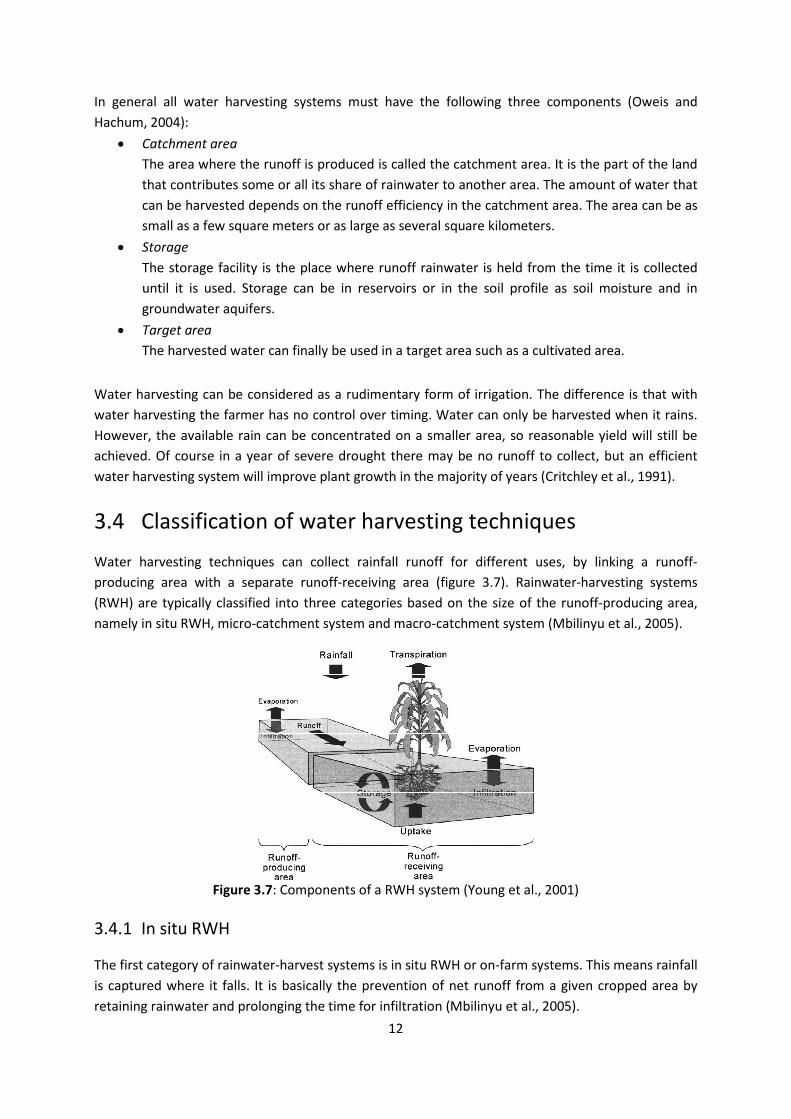
In general all water harvesting systems must have the following three components (Oweis and
Hachum, 2004):
• Catchment area
The area where the runoff is produced is called the catchment area. It is the part of the land
that contributes some or all its share of rainwater to another area. The amount of water that
can be harvested depends on the runoff efficiency in the catchment area. The area can be as
small as a few square meters or as large as several square kilometers.
• Storage
The storage facility is the place where runoff rainwater is held from the time it is collected
until it is used. Storage can be in reservoirs or in the soil profile as soil moisture and in
groundwater aquifers.
• Target area
The harvested water can finally be used in a target area such as a cultivated area.
Water harvesting can be considered as a rudimentary form of irrigation. The difference is that with
water harvesting the farmer has no control over timing. Water can only be harvested when it rains.
However, the available rain can be concentrated on a smaller area, so reasonable yield will still be
achieved. Of course in a year of severe drought there may be no runoff to collect, but an efficient
water harvesting system will improve plant growth in the majority of years (Critchley et al., 1991).
3.4 Classification of water harvesting techniques
Water harvesting techniques can collect rainfall runoff for different uses, by linking a runoff-
producing area with a separate runoff-receiving area (figure 3.7). Rainwater-harvesting systems
(RWH) are typically classified into three categories based on the size of the runoff-producing area,
namely in situ RWH, micro-catchment system and macro-catchment system (Mbilinyu et al., 2005).
Figure 3.7: Components of a RWH system (Young et al., 2001)
3.4.1 In situ RWH
The first category of rainwater-harvest systems is in situ RWH or on-farm systems. This means rainfall
is captured where it falls. It is basically the prevention of net runoff from a given cropped area by
retaining rainwater and prolonging the time for infiltration (Mbilinyu et al., 2005).

13
3.4.2 Micro-catchment system
The micro-catchment system is a second category of RWH system. It involves a distinct division
between a runoff-generating catchment area (CA) and a cultivated basin (CB) where the runoff is
stored in the root zone and productively used by plants. This principle is given in figure 3.7. The CA
and CB are adjacent to each other in a micro-catchment system (Mbilinyu et al., 2005).
The catchment length is usually between 1 and 30 meters and the ratio between CA and CB is
normally between 1:1 and 1:3 (Critchley et al., 1991). The farmer has control, within his farm, over
both the catchment and the target area. An example is shown in figure 3.8. This is an open-ended
structure in “V” shape. Runoff is collected and stored in the infiltration pit.
Figure 3.8: “V”-shaped micro-catchments (Critchley et al., 1991)
Micro-catchment systems provide many advantages over other irrigation techniques (Oweis and
Hachum, 2004):
• It is simple to construct.
• All the components are constructed within farm boundaries. This is an advantage from the
point of view of maintenance and management.
• It can be built rapidly using local materials and manpower.
• Runoff water does not have to be transported or pumped, so it is relatively inexpensive.
However, the principle of micro-catchment systems causes loss of productive land. Therefore it is
only practiced in the drier environments where cropping is most risky and farmers are willing to
allocate a part of their farm to be used as a catchment (Oweis and Hachum, 2004).
3.4.3 Macro-catchment system
The third category is macro-catchment system or an external catchment system, which is
characterized by having runoff water collected from relatively large CA’s. The catchment is usually 30
to 200 meters long and the ratio between CA and CB is usually between 2:1 and 10:1 (Critchley et al.,
1991). The catchment area is located outside the cropped area, where individual farmers have little
or no control over it (Mbilinyu et al., 2005). An example of a macro-catchment system is given in
figure 3.9. Trapezoidal bunds are used to enclose larger areas (up to 1 ha) and to impound larger
quantities of runoff. The name is derived from the structure (Critchley et al., 1991).

14
Figure 3.9: Trapezoidal bunds (Critchley et al., 1991)
The larger the size of the catchment the larger the distance runoff water has to surpass and the
lower the percentage of runoff collected. So the smaller individual catchments (micro-catchments)
have higher runoff efficiency (volume of runoff per unit of area). This is another advantage of micro-
catchments (Critchley et al., 1991).
3.5 The infiltration furrow
The infiltration furrow system is a micro-catchment system that is generally used for soil and water
retention in Chile. The main objectives of the use of the furrows are (CONAF and JICA, 1998b):
• Soil recuperation by catching the runoff water on slopes and thus reducing soil losses from
hillslopes.
• Increasing the infiltration of runoff water into the soil.
• Reduction of superficial runoff and its speed.
It is clear that infiltration furrows are a good tool to reduce land degradation hazards and because
more water infiltrates, there is more water available for plant production. This will increase the
survival chances of newly introduced plants.
The infiltration trench is a non-sloping channel that is dug out in a slope. This is done perpendicular
to the direction of the slope and parallel to the contour lines. In figure 3.10a an overview of the
implementation phase of infiltration trenches in catchment Quillay is shown. An example of an
infiltration furrow holding water is shown in figure 3.10b. The following specifications of the
infiltration furrow are recommenced by CONAF and JICA (CONAF and JICA, 1998b):
• A width at the top between 0.52 to 1 meter
• A width at the base of 0.2 meter
• A depth between 0.2 and 0.4 meter
• A length between 2.5 and 5 meter

15
(a) (b)
Figure 3.10: The infiltration furrow: a) Implementation of the trenches (CONAF and JICA, 1998b), b)
Example in catchment Quillay
The horizontal space between the infiltration trenches depends on the characteristics of the slope
(from eight meters in moderate slopes to three meters in moderate to steep slopes). The
construction cost of infiltration trenches can vary greatly depending on the configuration, location,
site-specific conditions, etc. The construction cost in catchment Quillay is 16950 Chilean pesos for
100 lineal meters per hectare or 24.67 euro for 100 lineal meters per hectare where 24 lineal meters
can be constructed each day (CONAF and JICA, 1999). In catchment Quillay the infiltration trenches
were implemented with the dimensions that are given in figure 3.11.
Figure 3.11: Dimensions of the furrows implemented in Quillay (After Tokugawa and Vargas, 1996)
16
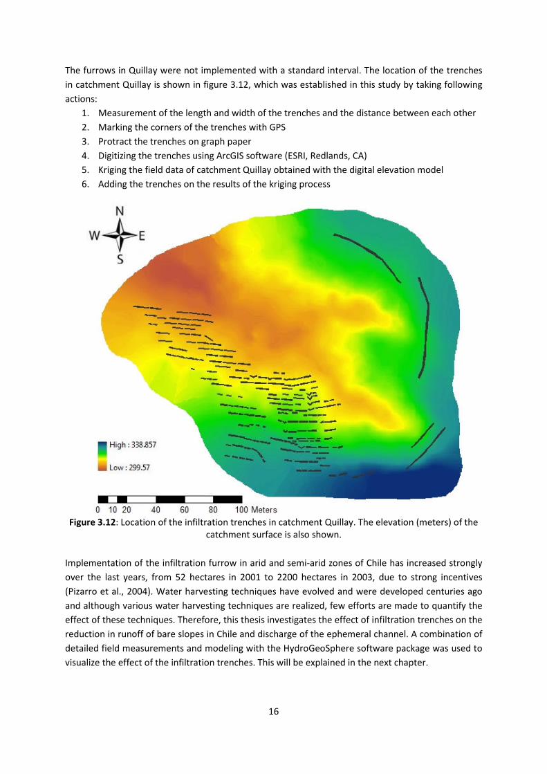
The furrows in Quillay were not implemented with a standard interval. The location of the trenches
in catchment Quillay is shown in figure 3.12, which was established in this study by taking following
actions:
1. Measurement of the length and width of the trenches and the distance between each other
2. Marking the corners of the trenches with GPS
3. Protract the trenches on graph paper
4. Digitizing the trenches using ArcGIS software (ESRI, Redlands, CA)
5. Kriging the field data of catchment Quillay obtained with the digital elevation model
6. Adding the trenches on the results of the kriging process
Figure 3.12: Location of the infiltration trenches in catchment Quillay. The elevation (meters) of the
catchment surface is also shown.
Implementation of the infiltration furrow in arid and semi-arid zones of Chile has increased strongly
over the last years, from 52 hectares in 2001 to 2200 hectares in 2003, due to strong incentives
(Pizarro et al., 2004). Water harvesting techniques have evolved and were developed centuries ago
and although various water harvesting techniques are realized, few efforts are made to quantify the
effect of these techniques. Therefore, this thesis investigates the effect of infiltration trenches on the
reduction in runoff of bare slopes in Chile and discharge of the ephemeral channel. A combination of
detailed field measurements and modeling with the HydroGeoSphere software package was used to
visualize the effect of the infiltration trenches. This will be explained in the next chapter.
17
Chapter 4
Materials and methods In the first section the HydroGeoSphere software will be explained which was used to visualize the
effect of the infiltration trenches. Before using it for evaluating this effect, the model first needed to
be calibrated and to that end PEST was used. How this was done will be explained in the second
section. The evaluation of the effect of infiltration trenches will not only be performed with
HydroGeoSphere, but also by comparing soil physical properties in both catchments. This is done via
field measurements and statistical analysis of the corresponding results. The latter is explained in the
third and fourth sections.
4.1 HydroGeoSphere
Models for water transport at the surface and subsurface are helpful tools for understanding physical
processes and for validating scientific hypotheses. Although the 'blueprint' for physically-based,
surface-subsurface models was first proposed over three and a half decades ago (Freeze and Harlan,
1969), its use has only become widespread in the past 15 years with the advent of inexpensive and
powerful computers (Sudicky et al., 2008). Surface and subsurface water flow models can be
differentiated into three classes: the uncoupled, the iterative coupled and the fully coupled models.
Examples of fully coupled models are InHM (Vanderkwaak, 1999), ParFlow (Kollet and Maxwell,
2006) and HydroGeoSphere (Therrien et al., 2010). These models take into account all components
of the hydrologic cycle and the governing equations for the surface and subsurface domains are
simultaneously solved. This is in strong contrast to the previous generation of models, in which the
equations were solved separately for each domain and were eventually assembled via iteration
(Sciuto and Diekkrüger, 2010).
The model used in this study is the integrated surface-subsurface, three dimensional, finite element
model HydroGeoSphere. It is a powerful numerical simulator specifically developed for supporting
water resource and engineering projects pertaining to hydrologic systems with surface and
subsurface flow and mass transport components (Therrien et al., 2010). The HydroGeoSphere model
has been successfully applied at a large range of scales, from relatively small scale subcatchments,
e.g. Sudicky et al. (2008), to larger watersheds, e.g. Li et al. (2008). As the scale increases the
computation time will increase. The HydroGeoSphere has definitely got the potential for small and
large scale hydrological studies and will increase even more in the future, because the computing
power of computers is getting stronger and these computers are also becoming more affordable. In
the following subsections a short overview of the main processes of the HydroGeoSphere software
used in this thesis are discussed. More detailed information can be found in Therrien et al. (2010).
Also a pre-processor called Grid builder was used to generate the plots of Testigo and Quillay. Finally
the necessary input and output files are handled. This is discussed in the last subsection.

18
4.1.1 Main processes
There are three fluxes occurring: subsurface, surface and interface flux. Because the implementation
of these fluxes is based on different equations, each flux will be discussed separately in the following
subsections. In the last subsection flow boundary conditions are discussed.
4.1.1.1 Subsurface flow
Flow transport in the porous medium is simulated in three dimensions using the Richards’ equation
for variably saturated subsurface flow (Therrien et al., 2010):
− ∇ ∙ � ��� + ∑ ��� ± � = � ��� ������
where �[� !"#$ %#&'] is the volumetric fraction of the total porosity occupied by the porous
medium and is always equal to 1 except when a second porous continuum is considered for a
simulation. The vector � is the fluid flux [L T-1] and is given by:
� = −) ∙ *+ ∇ �ψ + z�
where *+ = *+(��� represents the relative permeability of the medium [dimensionless] with respect
to the degree of water saturation �� [dimensionless]. Water saturation is related to the water
content � [dimensionless] according to �� = ../. Van Genuchten (1980) proposed the following
saturation-pressure relation:
�� = ��+ + �1 − ��+� 11 + | 3ψ |4567 8%9 ψ < 0
�� = 1 8%9 ψ ≥ 0
with the relative permeability given by:
*+ = ��=> ?1 − @1 − ��A 7⁄ C7DE
where
@F = 1 − A4C , H > 1
and where 'J is the pore-connectivity parameter and is equal to 0.5 for most soils, α [L-1] and β
[dimensionless] are van Genuchten parameters, Se is an effective saturation [dimensionless]:
�� = �KL6KLM��A6KLM�
where ��+ is the residual water saturation [dimensionless] and is related to the water content �
according to ��+ = .M./. ψ [L] in equation 4.2 is the pressure head and Z [L] is the elevation head. The
hydraulic conductivity tensor ) [L T-1] is given by:
) = OPQ R
where g is the gravitational acceleration [L T-2], µ is the viscosity of water [M L-1 T-1], R is the
permeability tensor of the porous medium [L²] and S is the density of water [M L-3]. ��� in equation
4.1 represents the volumetric fluid exchange rate [L3 L-3 T-1] between the subsurface domain and all
(4.2)
(4.3)
(4.4)
(4.5)
(4.6)
(4.7)
(4.1)

19
other types of domains supported by the model. It is positive for flow into the porous medium. Fluid
exchange with the outside of the simulation domain, as specified from boundary conditions, is
represented by Q [L3 L-3 T-1]. This is a volumetric fluid flux per unit volume representing a source
(positive) or a sink (negative) to the porous medium system. �� [dimensionless] is the saturated
water content and is assumed equal to the porosity n (Therrien et al., 2010).
The storage term forming the right-hand side of equation 4.1 is expanded in a way similar to that
presented by Cooley (1971) and Neuman (1973) to describe subsurface flow in the saturated zone.
They relate a change in storage in the saturated zone to a change in fluid pressure through
compressibility terms and they also assume that the bulk compressibility of the medium is constant
for saturated and nearly-saturated conditions. For unsaturated conditions it is assumed that the
compressibility effects on storage of water are negligible compared to effects of changes in
saturation. The storage term is expressed as follows:
��� ������ ≈ ���� �U�� + �� �KL��
where �� is the specific storage coefficient [L-1] (Therrien et al., 2010).
4.1.1.2 Surface flow
The overland flow is simulated using the two-dimensional Saint Venant equations, which consist of
three equations and are given by the following mass balance equation (Therrien et al., 2010):
�ф� W��� + ��XYZ�[���� + ��XY\�[���] + �^� ± �^ = 0
coupled with the momentum equation for the x-direction:
��� �_�^�^� + ��� �_�^E �^� + ��] �_�^_]^�^� + a�^ �[��� = a�0��0b − �8b�
and the momentum equation for the y-direction:
��� �_]^�^� + ��] �_]^E �^� + ��� �_�^_]^�^� + a�^ �[��� = a�0��0c − �8c�
where ф^ is a surface flow domain porosity that integrates flows over uneven surfaces, ℎ^ is the
water surface elevation [L] and is the sum of the land surface elevation z0 [L] and the depth of flow �^ [L], _�^ and _]^ are the vertically averaged flow velocities in the x and y directions [L T-1] and �^ is
a volumetric flow rate per unit area representing external sources and sinks [L T-1].
The variables �^� , �^] , �e� and �e] used in equations 4.10 and 4.11 are dimensionless bed and
friction slopes in the x and y directions. The friction slopes can be determined with the Manning, the
Chezy or the Darcy-Weisbach equations. Only the Manning equations will be explained as it was used
in this study. Information about the Chezy and the Darcy-Weisbach equations can be found in
Therrien et al. (2010). Using the Manning equation the friction slopes are determined by:
�e� = XYZ�XY/�fZg[�h i⁄
�e] = XY\�XY/�f\g[�h i⁄
(4.9)
(4.12)
(4.13)
(4.8)
(4.10)
(4.11)

20
where _�^ is the vertically averaged velocity [L T-1] along the direction of maximum slope s, nx and ny
are the Manning roughness coefficients [L-1/3 T] in the x and y directions. The momentum equations
4.10 and 4.11 can be simplified using equations 4.12 and 4.13 and this results in the following
equations:
_j� = −k^� �W���
_j] = −k^] �W��]
where k^� and k^] are surface conductances [L T-1] and are given for the Manning equations by:
k^� = [�g i⁄fZ
A[�W� ��⁄ ]l g⁄
k^] = [�g i⁄f\
A[�W� ��⁄ ]l g⁄
The diffusion-wave equation which the HydroGeoSphere software uses to simulate surface flows is
finally obtained by substituting equations 4.14 and 4.15 into the mass balance equation 4.9, which
give the following simplified equation:
mф0ℎ0mn − mmb @�^k^� mℎ0mb C − mmc @�^k^] mℎ0mc C + �^�0 ± �^ = 0
Equation 4.13 can also be written in vectorial notation:
− ∇ ∙ ��^�o� − �0� ± �0 = �ф�W���
where �o is the fluid flux [L T-1] and is given by: �o = −)o ∙ *+^ ∇ �d^ + z^�
where *+^ is a factor that accounts for the reduction in horizontal conductance from obstruction
storage exclusion [dimensionless] (Therrien et al., 2010).
4.1.1.3 Flow coupling
The subsurface and surface are complex systems that behave in a coupled manner. Therefore fully
coupled models such as HydroGeoSphere have a big advantage, namely a full coupling between the
surface and subsurface flow can be accomplished. The approach, used to define the water exchange
term between the two domains, uses a Darcy flux relation to transfer water from one domain to the
other. The flux is computed from the difference in hydraulic head between the two domains. It
assumes that the domains are separated by a (nonexistent) thin layer of porous material across
which water exchange will occur. The water exchange term is given by (Therrien et al., 2010):
�^� = qM)rr=sZtu �ℎ − ℎ^�
where a positive � [T-1] represents flow from the subsurface to the surface as determined by
equation 4.9, h is the subsurface water head [L] and ℎ^ is the surface water head [L], *+
[dimensionlesss] is the relative permeability for the exchange flux, )rr is the vertical saturated
hydraulic conductivity of the underlying medium [L T-1] and '��vℎ is the coupling length [L] (Therrien
et al., 2010). A low value of the coupling length coefficient represents a rapid exchange of flow
between the two domains and a low leakance factor or coupling length requires more computation
time (Sciuto and Diekkrüger, 2010).
(4.14)
(4.18)
(4.20)
(4.21)
(4.15)
(4.16)
(4.17)
(4.19)

21
4.1.1.4 Flow boundary conditions
In this study the boundary conditions were expressed in terms of flux (Neumann type). In particular,
rainfall and evapotranspiration were applied to the surface and no boundary conditions were
imposed for the bottom and lateral domains. Evapotranspiration is an important component of the
water balance and for this particular reason it is discussed here. Actual evapotranspiration is
modeled as a combination of plant transpiration wJ and of evaporation x� and affects both
subsurface and surface flow domains. Transpiration occurs within the root zone of the subsurface.
The rate of transpiration wJ is estimated using the following relationship (Therrien et al., 2010):
wJ = 8A�y��� 8E��� z{|1xJ − xv}f5
where 8A�y��� is a function of leaf area index [dimensionless], 8E��� is a function of nodal water
content [dimensionless], RDF is the time varying root distribution function, xJ is the potential or
reference evapotranspiration and xv}f is the canopy evapotranspiration that corresponds to the
evaporation of water intercepted by the canopy. The vegetation term is expressed as equation 4.23,
the root zone term is defined by equation 4.24 and the moisture content is expressed by 4.25:
8A�y��� = !&b~0, ! #[1, ��2 + �1 y���]�
z{| = � +��� ′��g′�l′ [� ′� +��� ′��M� [� ′
8E��� =�����
0 8%9 0 ≤ � ≤ ��J8� 8%9 ��J ≤ � ≤ �ev1 8%9 �ev ≤ � ≤ �^8� 8%9 �^ ≤ � ≤ �}f0 8%9 �}f ≤ ��
where:
8� = 1 − � .�t6 ..�t6.L>���
8� = 1 − ?.��6 ..��6.�D��
and where C1, C2 and C3 are fitting parameter [dimensionless], y+ [L] is the effective root depth, z’
[L] is the depth coordinate from the soil surface, 9� is the root extraction function [L3 T-1], ��J is the
moisture content at the wilting point, �ev is the moisture content at field capacity, �^ is the moisture
content at the oxic limit and �}f is the moisture content at the anoxic limit. Below the wilting point
moisture content transpiration is zero. Above that the transpiration increases to a maximum at the
field capacity moisture content. This maximum is maintained up to the oxic moisture content,
beyond which the transpiration decreases to zero at the anoxic moisture content. The roots will
become inactive due to lack of aeration when the available moisture is larger than the anoxic
moisture content (Therrien et al., 2010).
Evaporation from the soil surface and subsurface soil layers is expressed as follows if we assume that
evaporation occurs along with transpiration:
x� = 3∗�xJ − xv}f�[1 − 8A�y���]x{|�y��
(4.22)
(4.23)
(4.25)
(4.24)
(4.26)
(4.27)
(4.28)

where EDF is the evaporation distribution function that distributes the water extracted from the
evaporative zone along the evaporative depth
expressed as follow:
Where θe1 is the moisture content above which full evaporation can occur and
moisture content below which evaporation is zero.
represents the maximum quantity of water that can be
and the canopy storage parameter
4.1.2 Grid builder
The first step in applying HydroGeoSphere is grid generation for which Grid builde
was used for designing the grids of catchment
generated automatically in a two
dimensional grid (McLaren, 2007). This projection is do
phase. Although no general rules can be given about the optimal grid size, it is recommended to use
the finest grid balanced with the availability of data and the required computational time to
guarantee an accurate solution (Sciuto and Diekkrüger, 2010).
A digital elevation model was used to define
mesh representing the top of both catchments
Testigo constructed with Grid builder is given. The grid is refined near the river.
Figure 4.1: Two dimensional grid of Testigo with a refining near the river
22
where EDF is the evaporation distribution function that distributes the water extracted from the
evaporative zone along the evaporative depth Le [L] and α* is a wetness factor [dimensionless
the moisture content above which full evaporation can occur and
moisture content below which evaporation is zero. The interception storage capacity
represents the maximum quantity of water that can be intercepted by the canopy. It depends on LAI
and the canopy storage parameter Cint [L] and is given by (Therrien et al., 2010):
The first step in applying HydroGeoSphere is grid generation for which Grid builde
the grids of catchments Testigo and Quillay. The finite element grid is
in a two-dimensional plane and is projected in the vertical
grid (McLaren, 2007). This projection is done during the HydroGeoSphere
es can be given about the optimal grid size, it is recommended to use
the finest grid balanced with the availability of data and the required computational time to
(Sciuto and Diekkrüger, 2010).
A digital elevation model was used to define with Grid builder a two-dimensional, triangular
both catchments. In figure 4.1 the two dimensional grid of catchment
constructed with Grid builder is given. The grid is refined near the river.
: Two dimensional grid of Testigo with a refining near the river
where EDF is the evaporation distribution function that distributes the water extracted from the
is a wetness factor [dimensionless] and is
the moisture content above which full evaporation can occur and θe2 is the limiting
The interception storage capacity [L]
intercepted by the canopy. It depends on LAI
The first step in applying HydroGeoSphere is grid generation for which Grid builder (McLaren, 2007)
. The finite element grid is
dimensional plane and is projected in the vertical to form a three-
ne during the HydroGeoSphere pre-processing
es can be given about the optimal grid size, it is recommended to use
the finest grid balanced with the availability of data and the required computational time to
dimensional, triangular-element
4.1 the two dimensional grid of catchment
: Two dimensional grid of Testigo with a refining near the river
(4.29)
(4.30)

23
The grid of Quillay is given in figure 4.2 and is refined near the infiltration furrows. The infiltration
trenches were incised into the surface mesh by lowering the nodes 0.20 m. The grid of Quillay is a
much finer grid than Testigo. This higher refinement was done to obtain a good resolution, as shown
in the right part of figure 4.2
Figure 4.2: Two dimensional grid of Quillay with a refining near river and infiltration furrows
On these grids the field elevation data obtained with the digital elevation model was added and a
kriging interpolation process started. The results of these interpolations can be visualized with
external visualization software like Tecplot 360 and is given in figure 4.3 for catchment Testigo and in
figure 4.4 for catchment Quillay. The grids in figure 4.3 and 4.4 are the finest grids. In order to
compare simulations on these fine grids with simulations on coarse grids, a rectangular grid was
made with an element length of 25 m for Testigo and Quillay. The coarse grid of Testigo is given in
figure 4.5 and the coarse grid of Quillay is given in figure 4.6.
Figure 4.3: Tecplot 3D-visualization of the surface elevation (meters) of Testigo after kriging.

24
Figure 4.4: Tecplot 3D-visualization of the surface elevation (meters) of Quillay after kriging
Figure 4.5: Coarse grid of Testigo and tecplot 3D-visualization of the surface elevation (meters)
Figure 4.6: Coarse grid of Quillay and tecplot 3D-visualization of the surface elevation (meters)

25
4.1.3 Input and output files
There are four steps involved in solving a given problem using HydroGeoSphere:
1. Build the necessary input files for the pre-processor GROK
2. Run GROK to generate input data files for the actual processor HGS
3. Run HGS to solve the problem and generate output data files
4. Run the post-processor HSPLOT which generates output files suitable to be opened in Tecplot
4.1.3.1 Input files
All inputs are text-based files which can be written with every text editor such as notepad++, but
they are to be saved with a specific extension. The main input file is the grok-file (extension: *.grok).
This is a controlling file with a well-structured list of commands and data, specifying the conditions
that have to be simulated. All the different possible commands are listed in the HydroGeoSphere
manual (Therrien et al., 2010). An example of used grok-files for catchments Testigo and Quillay are
given in appendix A. It concerns a simulation for the rainfall event described in chapter 5 (§5.3.2),
namely the simulations which are based on the finest grids and with evapotranspiration data.
Among other things, precipitation and runoff data are added in the grok-file. Rainfall data was
obtained through the cooperation between CONAF and JICA. A pluviometer (see figure 4.7) and an
automated pluviometer with a tipping bucket system which was connected to a battery driven
pluviograph was used to measure the amount of precipitation. Trap-like ticks were recorded
whenever the bucket changed sides, once for every millimeter rain. The ticks had to be counted and
digitalized manually.
(a) (b)
Figure 4.7: The pluviometer used in catchment Quillay: a) Exterior of the pluviometer, b) Collection of
rainwater in a bottle
Next to precipitation data, runoff data is needed. This data was also obtained through the
cooperation between CONAF and JICA where runoff data was collected for both catchments Testigo
and Quillay. The runoff measurements were determined using a limnigraph (figure 4.8a). This is
based upon a V-shaped weir by constant measurements of the water level of the water passing the

26
triangle. A water level recorder (model: W-351, Yokogawa Weathac Corporation) was used to
measure the water height. An example of a measuring paper is shown in figure 4.8b, whereby a
continuous full line is drawn reflecting the height difference for every millimeter. The red line gives
the differences in height in mm and the green line in cm. Measurements of the water level were
performed from 1993 until 2006.
(a) (b)
Figure 4.8: Measuring the runoff: a) Limnigraph in catchment Quillay, b) Discharge observation
paper (after Geeroms, 2009)
The discharge was determined for both watersheds from the continuous water level measurements
using the following equation (Tokugawa and Vargas, 1996):
� = �A� �[ n&# ∝E �2 a ℎ� g�
where Q [m³ s-1] is the discharge, �[ the coefficient of discharge, ∝ [°] the bottom angle of the V-
shaped weir, g [9.81 m s-2] the gravitational acceleration and h [m] the water level.
The grok-file can also refer to other input files, such as the mprops-, oprops- and etprops-files. Also
the grid-files discussed in subsection 4.1.2 can be used as input file.
The mprops-file stands for material properties file (extension: *.mprops) and contains the data
related to the porous subsurface part of the model. A few examples are hydraulic conductivity,
porosity, specific storage … The oprops-file stands for overland properties file (extension: *.oprops)
and contains overland or surface properties such as the x friction, y friction and coupling length. Note
that this is actually not a surface nor a subsurface parameter. The used values of the parameters in
the mprops and oprops files in this study are discussed later in §5.3.1.
The etprops-file stands for evapotranspiration properties file (extension: *.etprops) and contains the
data related to evapotranspiration. For Testigo data was used of Acacia caven and grass. For Quillay
data was used of Acacia caven, grass and Eucalyptus globulus subsp. globulus. Using a GPS, the trees
had been marked and this is shown in figure 4.9. The top area in this figure is catchment Testigo and
the area underneath is catchment Quillay.
(4.31)

27
Figure 4.9: Trees in catchments Testigo (top) and Quillay (bottom)
The introduction of evapotranspiration in the model is done by assigning parts of the top layer of the
grid as evaporating elements. This is done via Grid builder using the data obtained from the GPS
(figure 4.9). The top elements were therefore subdivided. Evapotranspiration parameters of
Eucalyptus globulus subsp. globulus were assigned to the areas containing big trees (Acacia dealbata,
Cupressus arizonica, Eucalyptus camaldulensis, Eucalyptus globulus, Maytenus boaria, Pinus and

28
Quillay). Evapotranspiration parameters of Acacia caven were assigned to the areas containing little
trees (Acacia caven and Romero silvestre) and the areas in between received evapotranspiration
values of grass. This simplification was made because evapotranspiration data was not available for
each of the different tree species, but for the current structure there is still a distinction made
between large and small trees. As such there is still sufficient reality fed into the model. The
parameters that were needed to simulate the total evapotranspiration are given in table 4.1. The
values for grass and Eucalyptus were taken from Geeroms (2009) and Hingston et al. (1997). The
values for Acacia were taken from Hingston et al. (1997). Although some values were chosen
identical to those of Eucalyptus because of lack of information, these can be updated at a later stage
when they become available. The etprops-files of Testigo and Quillay are given in appendix B.
Table 4.1: Input values for introducing evapotranspiration in the model. Grass Eucalyptus globulus Acacia caven
Parameter Value Unit Value Unit Value Unit
Canopy storage parameter � ¡¢£� 0.04 m 0.00045 m 0.0005 m
Initial interception storage �¤¡¢£o � 0.04 m 0.0003 m 0.0005 m
Transpiration fitting parameters
C1 C2 C3
0.5 0.0 1.0
- - -
0.3 0.2 1.0
- - -
0.3 0.2 1.0
- - -
Transpiration limiting saturations
Wilting point Field capacity Oxic limit Anoxic limit
0.29 0.56 0.75 0.90
% sat % sat % sat % sat
0.29 0.56 0.85 0.95
% sat % sat % sat % sat
0.29 0.56 0.85 0.95
% sat % sat % sat % sat
Evaporation limiting saturations
Minimum �¥¦§� Maximum �¥¦¨�
0.25 0.9
% sat % sat
0.22 0.95
% sat % sat
0.22 0.95
% sat % sat
Leaf Area Index �©ª«� 1.0 - 2.5 - 2.5 - Root zone depth �©¬� 0.5 m 5 m 1 m Evaporation depth �©¦� 0.5 m 5 m 1 m
In figure 4.10 the grid of catchment Testigo is shown where the red elements represent Acacia caven
and the blue elements represent grass. This was done in a similar way for catchment Quillay but with
three evaporating elements (Acacia caven, grass and Eucalyptus globulus).
Figure 4.10: The grid of catchment Testigo with a distinction into two different evaporating elements,
namely Acacia caven (red) and grass (blue)

Besides adding the etprops-file,
model and this is done in the
computed from vegetation and climatic factors
given in figure 4.12. The following data
are required as input for the program:
• Latitude: 33° 41’ 00’’, longitude: 71° 12’ 00’’
• Minimum and maximum temperature and sunlight hours: figure
• Humidity: figure 4.11b and w
(b) (c)
Figure 4.11: The necessary input data for calculating the reference evapotranspirationMinimum and maximum temperature and sunlight hours
Figure 4.12: The monthly reference evapotranspiration
0
10
20
30
40
0
10
20
30
40
50
60
70
80
90
Jan
uar
y
Feb
ruar
y
Mar
ch
Ap
ril
May
Jun
e
July
Au
gust
Hu
mid
ity
(%)
0
2
4
6
8
10
Pre
cip
itat
ion
/ev
apo
tran
spir
atio
n(m
m d
-1)
29
the reference evapotranspiration xJ also needs to be included in the
model and this is done in the grok-file (see appendix A). The potential evapotranspiration was
computed from vegetation and climatic factors using a computer program called CROPWAT and is
following data, that were obtained via the Chilean water authority (DGA)
required as input for the program:
ongitude: 71° 12’ 00’’ and altitude: 165 m
Minimum and maximum temperature and sunlight hours: figure 4.11a
and wind speed: figure 4.11c
(a)
(b) (c)
: The necessary input data for calculating the reference evapotranspirationum temperature and sunlight hours, b) Humidity (%), c)
reference evapotranspiration Ep and precipitation in
sun (h) Tmin (°C) Tmax (°C)
Au
gust
Sep
tem
ber
Oct
ob
er
No
vem
ber
Dec
emb
er
0
50
100
150
200
250
300
350
Jan
uar
y
Feb
ruar
y
Mar
ch
Ap
ril
May
Jun
e
July
Win
d s
pee
d (
km d
-1)
Precipitation
needs to be included in the
(see appendix A). The potential evapotranspiration was
using a computer program called CROPWAT and is
obtained via the Chilean water authority (DGA),
(b) (c)
: The necessary input data for calculating the reference evapotranspiration: a)
, b) Humidity (%), c) Wind speed (km d-1)
in 2001 in Alto Loica
July
Au
gust
Sep
tem
ber
Oct
ob
er
No
vem
ber
Dec
emb
er
Evapotranspiration

30
A comparison between the evapotranspiration and the precipitation for Alto Loica in 2001 is also
given in figure 4.12. The rainfall is negligible except for the months April, May, June, July and August.
The monthly reference evapotranspiration exceeds the monthly rainfall mostly from October through
April (Fujieda and Vargas, 2005).
4.1.3.2 Output files
A description of each of the output files generated by GROK en HGS fall outside the scope of this
study. More information about these files can be found in the HydroGeoSphere manual (Therrien et
al., 2010). Only the output files that are generated by the post-processor are of interest. These
output files can be visualized via Tecplot 360 or can be opened with Microsoft Excel, notepad++. In
figure 4.13 the Tecplot visualization in three dimensions of the pressure head of catchment Testigo is
given for day 199. The Tecplot visualization of catchment Quillay for day 199 is given in figure 4.14.
Figure 4.13: Tecplot 3D-visualization of Testigo with a simulation of the pressure head (meters)
Figure 4.14: Tecplot 3D-visualization of Quillay with a simulation of the pressure head (meters)

31
4.2 PEST PEST is a nonlinear parameter estimation and optimization modeling software for automated
calibration and data interpretation of models. The purpose of PEST (which is an acronym for
Parameter ESTimation) is to assist in data interpretation, model calibration and predictive analysis
(Doherty, 2010). PEST’s role in sensitivity analysis and predictive analysis is discussed in Pierreux
(2009). PEST was only used in this study for its role in model calibration. How PEST is used for
calibrating a model is explained in subsection 4.2.1. The soil water distribution as measured by the
TDR-probes and runoff rates during a rainfall simulation can be used as datasets for calibration and
this will be discussed in subsection 4.2.2.
4.2.1 Model Calibration
Models produce numbers. If there are field or laboratory measurements corresponding to some of
these numbers, PEST can adjust model parameters in order that the discrepancies between the
pertinent model-generated numbers and the corresponding measurements are reduced to a
minimum (Doherty, 2010). So when PEST is used for calibrating a model, it strives for a minimum
value of the objective function by implementing the Levenberg – Marquardt minimization procedure
(Marquardt, 1963).
The objective function mathematically expresses the discrepancy between the predicted system and
the observed values. The general form of the objective function Φ is as follows (Šimůnek et al.,
1998):
Φ�β� = ∑ _ ∑ °,¯1�∗�n°� − �¯�n° , H�5Ef±°²A�²A
where β is the vector of adjustable parameters (e.g., α, n, k� …), m the number of different
measurements sets, #¯ the number of measurements in a particular data set, �∗�n°� are specific
measurements at time n° for the jth measurement set, �¯�n° , H� are the corresponding model
predictions, _ and °,¯ are weighing coefficients. The weight °,¯ contains information about the
measurement error such that:
°,¯ = A³´µg
where σ·E is the variance of the measurement error of �∗. Often it is set equal to unity because of a
lack of information on the measurement variance (Šimůnek et al., 1998). _ is expressed as follows:
_ = A
PEST does the minimization process by taking control of the model and running it as many times as
necessary to achieve the minimum value of the objective function in order to determine the optimal
set of parameters. Here it is important that the model user informs PEST where the adjustable
parameters can be found in the model input files (Doherty, 2010).
(4.32)
(4.33)
(4.34)

32
More specifically, the Levenberg – Marquardt algorithm is an iterative procedure that PEST utilizes to
fit the parameters. The method starts with an initial estimate H° of the unknown parameters. In
many cases the algorithm converges only if the initial guess is already somewhat close to the final
solution. At the beginning of each iteration the relationship between model parameters and the
model generated observations is linearised by formulating it as a Taylor expansion about the
currently best parameter set at that point, by which the derivatives of all observations with respect
to all parameters must be calculated. This linearised problem is then solved for a better parameter
set and the new parameters are tested by running the model again. At every step the objective
function is calculated and compared to its previous value. Based on whether an improvement has
been achieved or not, PEST can decide to undertake another optimization iteration, or not. The
strength of this method lies in the fact that it estimates parameters using fewer model runs than any
other estimation method (Bahremand and De Smedt, 2007). This is a big advantage for large models
whose run times may be considerable. For further information about PEST, the reader is referred to
the manual (Doherty, 2010). For further information about improvement of this PEST parameter
estimation algorithm, the reader is referred to Goegebeur and Pauwels (2006).
4.2.2 Rainfall simulation
The soil water distribution as measured by the TDR-probes and runoff rates, both obtained during
rainfall simulation experiments in catchment Quillay, can be used as datasets for calibration. The aim
was to perform calibration so that a selection could be made as to which parameter set was most
suitable for testing the efficiency of infiltration trenches. The primary purpose of the rainfall
simulator was to accurately and precisely simulate natural rainfall.
4.2.2.1 Set-up of the rainfall simulator
The rainfall simulator (figure 4.15a) consists of a sprinkler boom on which nozzles (type Teejet TG SS
14w) were fixed at a distance of 1 meter from each other. The spraying system is supported by
metallic tripods with adjustable legs. The construction was positioned at a height of 1.8 meter.
(a) (b)
Figure 4.15: The rainfall simulation set-up: a) Set-up rainfall simulation, b) Determining the runoff
During the simulated rainfall event, the time for the wetting front to reach the four TDR probes was
monitored. The TDR probes were installed horizontally at a depth of 5 cm and a distance of 20 cm of
each other (figure 4.16). The rainfall simulation provides valuable information about the cumulative

33
infiltration characteristics, the amount of runoff produced and the field saturated hydraulic
conductivity Kfs (Verbist et al., 2009). To assure uniformity of the rainfall intensity and drop size
distribution, a preferential combination of 180 cm and 100 kPa for respectively height and pressure
was used (Alaerts, 2006).
Four rainfall events were simulated for 30 minutes. The rainfall amount and intensity was measured
by placing 14 cups with an inner diameter of 9.19 cm at the border of the plots (figure 4.16). The
intensity and the amount of rainfall were calculated from the average volume of water collected in
these cups during the simulation. Table 4.2 shows the slope of the four plots and the amount and
intensity of rainfall. A ditch around the plot drained the water that did not fall onto the plot.
Table 4.2: Slope, intensity and total amount of rainfall of the four rainfall events
Slope (%) Intensity (mm h-1
) Total amount of rainfall (mm)
Rainfall event 1 20.04 113.61 56.81 Rainfall event 2 27.56 118.38 59.19 Rainfall event 3 18.44 126.70 63.35 Rainfall event 4 17.96 111.57 55.79
Figure 4.16: Determining the rainfall intensity by using 14 cups
The water that did not infiltrate into the soil and ran off was collected by placing a cup at the end of a
pipe connected to a collection gutter (see figure 4.15b). The plot size for the runoff experiment was 1
x 1 m. After every minute we counted how many cups could be filled during that minute (each cup
had a volume of 700 ml) and total runoff was calculated during each minute. The evolution of runoff
with time for rainfall event 1 is given in figure 4.17. This figure shows that runoff was not constant.
This is due to the fact that the pressure of 100 kPa was not always achieved, because sometimes the
pump was less effective.
Figure 4.17: Average runoff for rainfall event 1
4.2.2.2 Time Domain Reflectrometry
A very accurate and easy method used for determining the volumetric water content is Time Domain
Reflectrometry (TDR). TDR is a method by which volumetric water content is estimated indirectly by
0
500
1000
1500
2000
2500
0 5 10 15 20 25 30
Ave
rage
ru
no
ff (
cm³)
Time (minutes)

34
measurement of the permittivity or dielectric constant of the soil. A TDR set-up consists of a pulse
generator, a transmission line, a timing unit and in case of the TDR100 (Campbell Scientific,
Loughborough, Logan, USA), which we used in this study, PCTDR software to read the wavelength.
This transmission line (figure 4.18) consists of a coaxial cable and a probe. The probe consists of
stainless, evenly spaced steel rods (Jury and Horton, 2004).
Figure 4.18: Schematic representation of a TDR transmission line (CSC, 2011)
The generator emits a high frequency electromagnetic wave, which is transmitted through the
coaxial cable towards the probe. At the junction between the cable and the probe, the pulse is
partially reflected back. The refracted pulse moves along the probe into the soil and is then reflected
to the source, where its travel time can be estimated with the software (Jury and Horton, 2004). The
velocity of the reflected pulse C [L T-1] is determined as follows (Cornelis, 2010):
� = E ¹�
where L is the length of the probe and T is the time interval between two subsequently reflected
pulses. The relative dielectric permittivity º+ [-] of the soil is calculated as follows (Cornelis, 2010):
ε¼ = 3 @�0� C2
where C0 [L T-1] is the velocity of electromagnetic waves in vacuum space and 3 [dimensionless] is a
factor depending on the shape of the probe. The permittivity relates to a material’s ability to
transmit an electric field. The dielectric permittivity for water is 80.36, for air one and for solid soil
particles around three. Therefore the higher the volumetric water content, the higher the dielectric
permittivity (Cornelis, 2010). Various equations exist that determine the volumetric water content or
θv [dimensionless] from εr. Topp et al. (1980) used the following empirical third-order polynomial to
calculate θv and this equation is quite universal and is mostly independent of the soil type:
�X = −5.3 × 10⁶E + 2.92 × 10⁶E εr − 5.5 × 10⁶� εrE + 4.3 × 10⁶Ã εr�
The volumetric water content (the volume of liquid water per volume of soil) obtained through the
four TDR probes for rainfall event 1 is given in figure 4.19.
Figure 4.19: Volumetric water content for rainfall event 1
0.15
0.2
0.25
0.3
0.35
0.4
0 5 10 15 20 25 30
Vo
lum
etri
c w
ater
co
nte
nt
(-)
Time (minutes)
TDR1
TDR2
TDR3
TDR4
(4.35)
(4.36)
(4.37)

35
4.3 Field measurements
The field saturated soil hydraulic conductivity was calculated via Guelph permeameter
measurements and will be explained in the first subsection. Infiltration measurements can also be
performed with the tension disk infiltrometer and will be explained in the second subsection. Soil
moisture characteristics can be determined through the analysis of undisturbed soil samples and is
explained in the last subsection. Finally, the methods used to see whether there are significant
differences between the results of the field measurements of the two catchments are discussed.
4.3.1 Guelph permeameter
The Guelph permeameter (GP) (Soil moisture Equipment Corp., Santa Barbara, USA) is an in-hole,
constant-head permeameter employing the Mariotte principle to maintain a constant water height in
a bore hole. The set-up of a GP on the field is given in figure 4.20a and the principle in figure 4.20b.
The GP consists of two reservoirs. The inner reservoir finds itself inside the outer reservoir. The inner
reservoir can be used when making readings in slow infiltration soils, to make sure a good resolution
is accomplished. Within the inner reservoir, a centric air tube is provided. After boring a hole the GP
is placed. Initially both reservoirs will be filled with water and a constant head level is established by
regulating the position of the bottom of the air tube. In these measurements the height was fixed at
5 cm. The water will flow slowly from the GP into the hole and penetrates into the soil. As the water
level in the reservoirs falls, a vacuum is created in the air space above the water, at the top of the GP.
This vacuum can only be relieved when air of ambient atmosphere pressure enters the reservoirs
through the air inlet tip and bubbles up towards the top of the reservoir.
(a) (b)
Figure 4.20: Field determination of the hydraulic conductivity using the Guelph permeameter: a) Set-
up, b) Principle of the Guelph permeameter
At a certain moment a saturated bulb is formed and the flow of water from the storage cylinder
reaches a constant and measurable value. These data together with the diameter of the hole and the
water level in the hole were used to determine the saturated hydraulic conductivity. The field
saturated hydraulic conductivity Kfs [L T-1] was calculated as follows (Elrick and Reynolds, 1992):

36
ke� = � Ä/E ŠƲÈ� Å }²Èg É ÊË∗
where �� [L³ T-1] is the steady state water discharge when a constant depth of ponding H [L] is
maintained in the well, C is a dimensionless shape factor that depends primarily on the H/a ratio, a is
the radius of the well [L] and 3∗ [L-1] is a soil texture-structure parameter. The term “field-saturated”
is used because under field conditions air is usually entrapped in the soil during the infiltration
process and this can result in estimates of the “saturated” hydraulic conductivity. The field saturated
hydraulic conductivity is lower than if the soil had been completely saturated (Elrick et al., 1989).
The 3∗ parameter is the soil macroscopic capillary length parameter and represents the importance
of gravity and capillarity forces during an infiltration process (Raats, 1976). A large 3∗ value indicates
a dominance of gravity over capillarity. According Elrick et al. (1989) 3∗ is equal to 0.04 cm-1 for soils
that are both fine textured and unstructured. Since this is the case for the studied area, a value of
0.04 cm-1 was taken which is a rather low value (dominance of capillarity over gravity). In this case H
was 0.05 meter and a was 0.03 meter. From the onset of the infiltration experiment, every 2 minutes
the change of the water level in the reservoir was recorded and this during 60 minutes. The
difference between the water level values of each subsequent measurement period was then
calculated. Finally, the average of the infiltration values of the last ten minutes was calculated and
divided by the measurement period (2 minutes). Hereafter �� was calculated by multiplying this
mean infiltration rate with the cross section of the inner and outer (X = 35.22 cm²) or inner (Y =2.15
cm²) reservoir. In these measurements the inner and outer reservoir was used and therefore �� was
calculated using the X value. The C-factor was calculated with the empirical formula of Zhang et al.
(1998). For 3∗ ≥ 0.04 cm-1 and when 0.25 < Æ} < 20 the factor is calculated as follows:
� = @ ÆA.ÌÌE }È^.^ÌA ÆC^.Ã��
Measurements for the field satured hydraulic conductivity were done at a depth of 30 cm beneath
the soil surface. This was done twelve times, six in catchment Testigo and six in catchment Quillay.
Where the Guelph measurements were taken in the catchments are given in figure 4.22 and 4.23.
4.3.2 Tension disk infiltrometry
Tension disk infiltrometry is a popular method for in situ measurement of the unsaturated soil
hydraulic properties. The tension infiltrometer (Soil moisture Equipment corp., Santa Barbara, USA)
(figure 4.21c) is an instrument to characterize water entry into the soil under a range of negative
water pressure heads (Verbist et al., 2009). By filling the inlet tube (figure 4.21d) with a given height
of water, a counter head is created. This counter head only allows water to infiltrate into pores that
are able to exert a suction that is higher than the pressure head at the inlet. Therefore at large
negative pressure heads, water only flows through very small pores. As the pressure head is
increased towards zero pressure head, larger pores participate to flow.
Prior to putting the device into position in catchment Quillay, the soil surface was leveled (figure
4.21a by the use of a shovel, to ensure the device could stand up straight. Next, contact sand was
used to obtain optimal contact between the disk (figure 4.21d) and the soil. The desired pressure
(4.38)
( 4.39)

37
head was established by varying the volume of water within the tube (figure 4.21d on the left). This
tube is directly connected to the disk. For each measurement (10 in total), subsequent pressure
heads were used: -0.12 m, -0.09 m, -0.03 m and -0.001 m. If the soil was relatively wet then the
following subsequent pressure heads were used: -0.10 m, -0.07 m, -0.03 m and -0.001 m. For each
pressure head, the measurements proceed in analogy with the Guelph permeameter. Before the
measurement could begin, the air tube was pulled up to 5 cm. The measurements started when the
first bubbles of air passed through the disc and visibly rose in the reservoir. The readings of the
cumulative infiltration were done manually every minute during one hour. The moisture content was
determined using the TDR probes before and after the tension disk infiltrometry (figure 4.21b).
(a) (b)
(c) (d)
Figure 4.21: Field determination of the hydraulic conductivity using the tension disk infiltrometer: a)
Leveling the top layer, b) TDR measurements, c) Tension disk infiltrometer, d) disk of a tension infiltrometer
After conversion of the reading values into steady state infiltration rates � �ℎ� [L³ T-1], the
corresponding unsaturated hydraulic conductivity at different imposed pressure heads was
calculated by invoking Ankeny’s et al. (1991) equations:
� �ℎA� = @Í 9E + + ∗ E ∗[ ℎ1− ℎ2] ∗ [��ℎ1�+��ℎ2�][��ℎ1�−��ℎ2�] C k�ℎA�
k�ℎE� = Ä�Wg�∗ Î�Wl�Ä�Wl�
(4.40)
(4.41)

38
with 9 [L] is the radius of the disc, h1 and h2 [L] are two pressure heads (with h1 the highest pressure
head), ��ℎA� and ��ℎE� are two steady state infiltration rates respectively at pressure head 1 and 2, k�ℎA� and k�ℎE� are the unsaturated hydraulic conductivities respectively at pressure head 1 and 2.
In this case r was 0.1025 meter and the applied pressure heads are mentioned in previous paragraph.
From the onset of the experiment, every minute the change of the water level in the reservoir was
recorded. After fifteen minutes another pressure head was selected. The difference between the
water level values of each subsequent measurement period (1 minute) was then calculated for each
pressure head. Finally the average of the infiltration values of the last five minutes was calculated for
each pressure head. The steady state infiltration rates � �ℎ� were then calculated by multiplying
these mean infiltration rates at each pressure head with the cross section of the inner and outer (X =
35.22 cm²) or inner (Y =2.15 cm²) reservoir. As with the Guelph measurements also here the inner
and outer reservoir was used.
4.3.3 Soil moisture characteristics
Thirty undisturbed soil samples were taken using standard 100cm³ Kopecky rings at a depth of 35 cm
beneath the soil surface to determine the soil water retention curves i.e. the relationship between
the soil water content θ [m³ m-3] and the matric potential Ï� in pressure units [Pa] or h in hydraulic
head units [m]. The matric potential can be defined, according Jury and Horton (2004), as the energy
per unit volume of water required to transfer an infinitesimal quantity of water from a reference
pool of soil water at elevation of the soil to the point of interest in the soil at reference air pressure.
For the determination of the soil water retention curve fifteen soil samples (figure 4.22) were taken
at catchment Quillay. Three transects were drawn and on each transect five soil samples were taken.
The blue line represents the river and the three transects are the three pink lines. Also the six Guelph
measurements are shown in this figure.
Figure 4.22: Taken soil samples and Guelph measurements in catchment Quillay, obtained via ArcGIS
The other 15 samples were taken in the catchment Testigo (see figure 4.23). The same method was
used as in catchment Quillay and the 10 Guelph measurements are also given in figure 4.23.

39
Figure 4.23: Taken soil samples and Guelph measurements in catchment Testigo, obtained via ArcGIS
The 30 samples were analyzed in the laboratory of the Department of Soil Management, Faculty of
Bioscience Engineering, Ghent University, to determine the soil water retention curves. In the
laboratory the samples were subjected to the under-pressure method with sandbox (Eijkelkamp
Agrisearch Equipment, Giesbeek, the Netherlands) for pressure heads of -10 cm, -30 cm, -60 cm and
-100 cm and the overpressure method was used with ceramic plates (Soilmoisture Equipment
Corporation, Santa Barbara, CA, USA) for pressures of -33, -100 and -1500 kPa. For a more profound
description of the used method the reader is referred to the manual of methods for soil analysis of
the above laboratory (Gabriels et al., 1998). The equation that was used to describe the relationship
between the soil water content and the matric potential was the closed form equation of van
Genuchten (1980) (see eq. 4.3).
In accordance with van Genuchten et al. (1991) the restriction m = 1 − Af was imposed. Hereby is n
the H parameter in eq. 4.3. The parameters of the van Genuchten equation (�+, ��, n, 3, Ks) were
estimated via the iterative algorithm of Marquardt (Marquardt, 1963) by using the RETC-software by
van Genuchten et al. (1991). According to Geeroms (2009) the necessary initial estimates of the van
Genuchten parameters are those corresponding with a Sandy Clay Loam soil as soil textural group.
Carsel and Parrish (1988) was used to determine initial estimates for this soil type, resulting in values
of �+ equal to 0.100 m³ m-3, �� is 0.39 m³ m-3, n is 1.48 m³ m-3, 3 is 0.059 cm-1 and Ks is 31.44 cm d-1
for non linear curve fitting.
4.3.4 Statistical analysis
In order to evaluate and compare the different results of the field measurements a statistical
evaluation procedure was carried out. For in situ measurements of hydraulic conductivities it is
common that the calculated saturated hydraulic conductivities show lognormal statistical
distributions when tested using a Kolmogorov-Smirnov test (e.g. Warrick and Nielsen, 1980). As a

40
result all statistical analysis with the Guelph permeameter were performed on lognormal
transformed hydraulic conductivities and to be sure a Kolmogorov-Smirnov test was used to see
whether this is true via the statistical software program SPSS (IBM, Armonk, New York). If the Asymp.
Sig. (2-tailed) value in the output of SPSS was greater than the level of significance (often 0.05 is
used) the distribution was normal.
These logs normally transformed Kfs were subjected to an independent two-sample T-test with SPSS.
This T-test compares the mean scores of two groups on a given variable. There are a few
assumptions:
• The dependent variable is normally distributed.
• The two groups have approximately equal variance on the dependent variable.
• The two groups are independent of one other.
The Levene’s test was used to confirm the statistical requirement of equal variances
(homoscedasticity). If the Levene’s Test is significant (p<level of significance), the two variances are
significantly different. Also here 0.05 was used as level of significance and when p>0.05 the variances
are approximately equal. The second assumption is met. After performing a Levene’s test for equality
of variances, a T-test for equality for means was carried out.
It is also possible to investigate whether there is a significant difference between more than two
groups. The independent two-sample T-test cannot be used in this case (only 2 groups are possible).
Therefore a one-way ANOVA was used, because it is an extension of the independent two-sample T-
test and therefore more than 2 groups can be used to compare the means of them on a given
variable. The one-way ANOVA has the same assumptions as the independent two-sample T-test. The
same level of significance was, namely 0.05.
Also the other results of the field measurements (tension disk infiltrometry and soil samples) were
subjected to the same statistical analysis as mentioned above.

41
Chapter 5
Evaluation of the effect of the infiltration trenches in Alto Loica In the following sections the use of the implemented infiltration trenches in Quillay (as earlier
mentioned in the literature review) was evaluated by comparing Testigo and Quillay. This
comparison was done via three ways: i) by comparing measurements of the rainfall and discharge
obtained by CONAF and JICA, ii) by comparing soil physical properties in both catchments (field
measurements) and iii) by comparing via modeling.
5.1 Evaluation based upon discharge measurements The precipitation and discharge in Testigo in 2001 is given in figure 5.1. The runoff was measured
only from May 14 (day 134) until October 7 (day 280) with the limnigraph. It can be seen that a
runoff peak corresponds perfectly to a rainfall peak except between June 12 (day 163) and June 22
(day 173) (red arrow in figure 5.1) during which the limnigraph did not work. When the precipitation
decreased from that of the previous days, the discharge decreased slowly. Conversely, when
precipitation peaks followed each other quickly, the soil became saturated and at the next rainfall
peak the runoff peak was higher. This is the case for day 210 and day 211. Figure 5.1 shows also a
comparison between the discharge in Quillay and Testigo. The limnigraph in Quillay did not work
from August 26 (day 238) until September 4 (day 247). Hence, there is no runoff peak visible in the
figure from August 26 to September 4. The effect of the furrows can be observed in lower discharge
peaks. For example, on day 210 the runoff in Testigo was almost 5 times higher than in Quillay.
Figure 5.1: Comparison between the discharge with and without treatment in 2001. The
corresponding precipitation is also given.
0.0
10.0
20.0
30.0
40.0
50.0
60.0
70.0
13
4
13
9
14
4
14
9
15
4
15
9
16
4
16
9
17
4
17
9
18
4
18
9
19
4
19
9
20
4
20
9
21
4
21
9
22
4
22
9
23
4
23
9
24
4
24
9
25
4
25
9
26
4
26
9
27
4
27
9Pre
cip
itat
ion
/ d
isch
arge
(m
m d
-1)
DayPrecipitation Discharge without treatment Discharge with treatment

42
If the discharge is expressed on a logarithmic scale, a delay in runoff travel time due to the infiltration
trenches can clearly be seen for catchment Quillay in contrast with catchment Testigo. This is shown
in figure 5.2.
Figure 5.2: Comparison on logarithmic scale between discharge with and without treatment in 2001
The same effect was found for the year 1998 (dry year) and 1997 (wet year). A rain event of the
driest year of the measurements, namely 1998 was selected (11 September). The precipitation of this
event and the corresponding runoff in catchments Testigo and Quillay is given in figure 5.3. Runoff
was still observed in catchment Testigo (untreated watershed) while no runoff was produced in
catchment Quillay with soil and water conservation measures. This means that the precipitation was
stored in the watershed Quillay and therefore increased the plant available water in a dry year.
Figure 5.3: The discharge (m³) in catchments Testigo and Quillay from the rain event of 11 September
in 1998. The corresponding precipitation (mm) is also given.
A rain event – 3 until 5 October - was also selected for the year 1997 which was a wet year and the
discharge of both catchments Testigo and Quillay were calculated and plotted. This is shown in figure
5.4. The corresponding discharge is also shown in figure 5.4. From this graph, convincing evidence
could be found that the infiltration furrows have an effect in reducing peak runoff. A large effect can
be observed of the introduced treatment. The runoff peaks are reduced to more than a half of the
values that were observed where no water harvesting techniques were implemented.
0.0
0.1
1.0
10.0
100.0
13
4
13
9
14
4
14
9
15
4
15
9
16
4
16
9
17
4
17
9
18
4
18
9
19
4
19
9
20
4
20
9
21
4
21
9
22
4
22
9
23
4
23
9
24
4
24
9
25
4
25
9
26
4
26
9
27
4
27
9
Pre
cip
itat
ion
/ d
isch
arge
(m
m d
-1)
DayPrecipitation Discharge without treatment Discharge with treatment
024681012141618200
0.2
0.4
0.6
0.8
1
1.2
0 1 2 3 4 5 6 7 8 9 10 11 12 13 14 15 16 17 18 19 20 21 22 23 24
Pre
cip
itat
ion
(m
m)
Ru
no
ff (
m³)
HoursPrecipitation Testigo Quillay

43
Figure 5.4: Comparison between the discharge (m³) in catchments Quillay and Testigo from the rain
event of 3 until 5 October in 1997. The corresponding precipitation (mm) is also given.
A second rain event in the same wet year 1997 (29 until 30 July) and the corresponding hydrographs
of catchments Testigo and Quillay are given in figure 5.5. This is a rain event whereby it has rained
more than the rain event in figure 5.4. In this rain event a lot of precipitation peaks followed each
other quickly and saturated the soil, because this next rainfall peak, namely after 32 hours, was high
(more than 160 m³). Even during such high rainfall event the infiltration furrows were able to reduce
the runoff peak with more than a half of the value that was observed in catchment Testigo, namely
60 m³. As a result, the idea is suggested that the measurements are able to withhold a big part of the
total amounts of precipitation, but not the total amount. According to Geeroms (2009) the latter is
explained by under-dimensioning of the system.
Figure 5.5: Comparison between the discharge in catchments Quillay and Testigo from the rain event
of 29 until 30 July in 1997. The corresponding precipitation (mm) is also given.
It is clear that the use of water harvesting techniques, such as the infiltration trenches, have an effect
on reducing the peak runoff. Nevertheless, some points of discussion have to be taken into account.
The first point that should be kept in mind is that there is a difference in size between catchment
Testigo (3.60 hectares) and catchment Quillay (2.80 hectares). This obviously has some impact on the
comparison between both catchments for evaluating the effect of the infiltration furrows. Therefore,
it has to be considered that small differences in peak runoff can be the result of the size difference
between the two catchments. But the clearly larger differences can be explained as the effect of the
infiltration furrows. Certainly, it is possible to avoid this first problem by dividing the runoff in m³ by
the surface are of the watershed, as done in figure 5.1 and 5.2. However, in this study was not opted
0.0
2.0
4.0
6.0
8.0
10.0
12.0
14.0 0
5
10
15
20
25
30
0 4 8
12
16
20
24
28
32
36
40
44
48
52
56
60
64
68
72
76
Pre
cip
itat
ion
(m
m)
Ru
no
ff (
m³)
HoursPrecipitation Testigo Quillay
0.0 2.0 4.0 6.0 8.0 10.0 12.0 14.0 16.0 18.0 20.0 22.0 24.0 26.0 0
153045607590
105120135150165180195210
0 2 4 6 8
10
12
14
16
18
20
22
24
26
28
30
32
34
36
38
40
42
44
46
48
Pre
cip
itat
ion
(m
m)
Ru
no
ff (
m³)
HoursPrecipitation Testigo Quillay

44
for this strategy for the following reason. The demarcation of the two catchments was very
subjective determined. Therefore different people suggests different surface areas of the two
watersheds, e.g. CONAF and JICA (1998) suggests a surface area of 3.60 hectares for Testigo and 2.80
hectares for Quillay, Verbist (2011) on the other hand suggests a surface area of 3.90 hectares for
Testigo and 3.80 hectares for Quillay. The surface are of the grids used in this study amounts to 5.11
hectares for Testigo and 3.83 hectares for Quillay. Thus, because of the subjectivity during the
demarcation the runoff was expressed in m³ or in m³ s-1 (see §5.3) and not in millimeter.
A second point is that a large range of treatments were introduced in catchment Quillay, including
the infiltration furrows. Therefore, it is possible that the effect of a reduction in peak runoff is the
result of not only the furrows, but also of the other implemented treatments such as the water
deviation channels and the plantation of trees. Nevertheless, the furrows were the main treatment,
so it can be expected that the effect of reduction in peak runoff was mainly due to the trenches.
5.2 Evaluation based upon field measurements
In this section a comparison of the Kfs and the Kh will be made between the two catchments to see
whether the infiltration furrows have impacted the soil properties. Finally, the soil moisture
characteristics of the two watersheds will be compared through the analysis of undisturbed soil
samples and determining the soil water retention curves to see if homogeneous conditions occurred
in both catchments.
5.2.1 Guelph permeameter
In table 5.1, the results of the calculations of the field saturated hydraulic conductivities or Kfs via the
twelve Guelph measurements (six in Testigo and six in Quillay) are given. First a Kolmogorov-Smirnov
test was performed to see whether the log (kfs) values are normally distributed in each catchment.
The output of the test is given in appendix C.1.1. The test indicated that the log (kfs) values were
normally distributed for Testigo as well as for Quillay. Therefore all statistical analysis can be
performed on lognormal transformed hydraulic conductivities. The output of the independent two-
sample T-tests and the one-way ANOVA can be found respectively in appendix C.1.2 and C.1.3.
Table 5.1: The calculated field saturated hydraulic conductivities via the Guelph measurements
Guelph measuring points (see figure 4.22 and 4.23) Kfs (m s-1
) Log (Kfs)
Catchment Testigo
1 2 3 4 5 6
1.259 E-11 3.776 E-11 1.290 E-10 2.612 E-10 9.440 E-12 1.259 E-11
-10.900 -10.423 -9.889 -9.583
-11.025 -10.900
Catchment Quillay
1 2 3 4 5 6
5.035 E-11 9.440 E-12 1.259 E-11 1.573 E-11 6.293 E-12 1.259 E-11
-11.025 -10.298 -10.900 -10.803 -11.201 -10.900

45
Catchment Testigo versus catchment Quillay
In this case the T-test compares the geometric mean log(Kfs) measured in catchment Testigo and
Quillay. In table 5.2, it is shown that the mean log (kfs) of Testigo is higher than Quillay’s. The levene’s
test was not significant (p=0.069) and the independent two-sample T-test showed no significant
difference between the log (kfs) of catchments Testigo and Quillay (p=0.176). This suggests that the
soil conservation measures, such as the infiltration furrows, had not impacted the soil properties
sufficiently to observe any measurable differences. This confirms the results of Daelman (2009), who
didn’t find any significant differences when using a tension infiltrometer.
Table 5.2: Group statistics
Catchment Number Mean Std. Deviation Std. Error Mean
log (Kfs) Testigo 6 (see table 5.1) -10.4534 .60039 .24511
Quillay 6 (see table 5.1) -10.8540 .30527 .12462
Slope aspect in each catchment
It can be investigated whether there is a significant difference between the mean log (kfs) values of
the western and the eastern part of the watershed Testigo. In table 5.3, it is shown that the mean log
(kfs) of the western part is the highest. The Levene’s test (p=0.299) indicated that variances are
approximately equal and no significant difference (p=0.865) was observed between the log (kfs) in the
western and the eastern part of the watershed. The same was done for catchment Quillay. Table 5.3
shows that the mean log (kfs) of the western part is the highest, therefore the same trend is
maintained as in Testigo. The Levene’s test (p=0.159) and the T-test (p=0.143) indicated the same
result as in catchment Testigo.
Table 5.3: Group statistics
N Mean Std. Deviation Std. Error Mean
log (Kfs) Catchment Testigo
East (measurement 4, 5 and 6) West (measurement 1, 2 and 3)
3 3
-10.5027 -10.4040
0.79890 0.50577
0.46125 0.29201
Catchment Quillay
East (measurement 1, 5 and 6) West (measurement 2, 3 and 4)
3 3
-11.0420 -10.6670
0.15122 0.32322
0.08731 0.18661
Between transects in each catchment
The one way ANOVA was performed on the log (kfs) resulting of the Guelph measurements taken in
Testigo (figure 23) and Quillay (figure 22). In table 5.4, it is shown that the log (kfs) of transect 3 is the
highest for Testigo. This is also the case for watershed Quillay, therefore the same trend is
maintained as in Testigo. The one-way ANOVA indicated that there was no significant difference
(p=0.805) between the mean log (kfs) of the three transects in Testigo. For catchment Quillay the
same conclusion was found (p=0.555).
Table 5.4: Group statistics
N Mean Std. Deviation Std. Error Mean
log (Kfs) Catchment Testigo
Transect 1 (measurement 3 and 6) Transect 2 (measurement 2 and 5) Transect 3 (measurement 1 and 4)
2 2 2
-10.3945 -10.7240 -10.2415
0.71488 0.42568 0.93126
0.50550 0.30100 0.65850
Catchment Quillay
Transect 1 (measurement 4 and 6) Transect 2 (measurement 3 and 5) Transect 3 (measurement 1 and 2)
2 2 2
-10.8515 -11.0505 -10.6615
0.06859 0.21284 0.51407
0.04850 0.15050 0.36350

46
5.2.2 Tension disk infiltrometry
In table 5.5 the group statistics are shown which resulted from the calculations of the unsaturated
hydraulic conductivities via the 10 tension infiltrometry measurements in catchment Quillay (see
table 5.6).
Table 5.5: Group statistics for catchment Quillay
Kh E-6 m s-1
N Mean Std. Deviation
K-0.001
K-0.03 10 10
13.2160 3.1200
6.68939 2.39850
K-0.09
K-0.12 10 10
1.1750 1.0210
0.88821 0.79981
Table 5.6: The calculated unsaturated hydraulic conductivities via the tension disk infiltrometry measurements
Tension disk infiltrometry
measurements
K-0.001
E-6 m s-1
K-0.03
E-6 m s-1
K-0.09**
E-6 m s-1
K-0.12*
E-6 m s-1
1
2
3
4
5
6
7
8
9
10
10.35
6.90
4.49
13.75
5.95
15.21
21.31
24.51
18.24
11.45
1.49
1.48
1.07
3.17
1.01
4.46
2.85
4.47
8.90
2.30
0.99
1.03
0.83
0.53
0.50
0.79
1.14
1.28
3.60
1.06
1.12
0.59
0.71
0.26
0.34
0.53
1.33
1.06
3.03
1.24
*For measurement 2, 3, 4 and 6 K-0.10 was used, ** For measurement 2, 3, 4 and 6 K-0.07 was used
These results can be compared with earlier studies, such as Verbist (2011) and Daelman (2009). In
these studies none of the conductivities proved significantly different between the two watersheds.
First a Kolmogorov-Smirnov test was performed to see whether the kh values are normally
distributed for each pressure head. The outputs of the tests are given in appendix C.2.1. The test
indicated that the kh values are normally distributed for each pressure head. To investigate if there is
a significant difference between the values in table 5.5 of Quillay and those of Testigo in Verbist
(2011) and Daelman (2009) a two-sample independent T-test was used. The outputs of these tests
are given in appendix C.2.2. Only the hydraulic conductivities at pressure heads -0.12 m, -0.03 m and
-0.001 m can be compared because in the 10 tension infiltrometry measurements done this year in
Quillay there were no measurements of hydraulic conductivities at pressure head -0.06 m.
All the two-sample independent T-tests indicated that there is significant difference between the
hydraulic conductivities of catchments Testigo and Quillay. The T-test can also be used to compare
the values of catchment Quillay obtained in 2010 (table 5.5) with the values of catchment Quillay
obtained by Verbist (2011) and Daelman (2009). Also here the T-test indicated a significant
difference. Based on current knowledge, no clear reason could be found that explains the measured
differences between both data sets.

47
5.2.3 Soil moisture characteristics
The van Genuchten parameters were estimated from fifteen undisturbed soil samples taken at a
depth of 35 cm in each catchment, using the methodology described in chapter 4 (§4.3.3). The
resulting soil water retention curve (figure 5.6 for catchment Testigo and figure 5.7 for catchment
Quillay) fitted rather well to the data.
Figure 5.6: Soil water retention curve with indication of mean and individual measurements for
catchment Testigo
Figure 5.7: Soil water retention curve with indication of mean and individual measurements for
catchment Quillay
From the soil-water retention curve, the available water capacity �ÑÒ� [m³ m-3] was estimated as the
difference between � at -33 kPa and � at -1500 kPa. This was done for both catchments and for each
transect within each watershed. The results are given in table 5.7. The Kolmogorov-Smirnov test
indicated that the �ÑÒ� are normally distributed in each catchment. No significant difference was
found between the �ÑÒ� of each catchment. Also, no significant difference was found between the
transects in each watershed. The corresponding outputs of the Kolmogorov-Smirnov test, T-tests and
the one-way ANOVA’s are given in appendix C3. In Daelman (2009) soil samples were already taken
at a depth of 5 cm in catchment Quillay. Also, here no significant differences were found between

48
�ÑÒ� inside and outside the trench. This shows the homogeneous conditions occurring in both
catchments, allowing them to be considered equal in terms of their hydrophysical properties.
Table 5.7: Available water capacity in catchments Testigo and Quillay
ÓÔÕÖ [m³ m-3
] ×Ø ± Ù
Catchment Testigo
Transect 1 Transect 2 Transect 3
0.0679 ± 0.02653 0.0569 ± 0.01004 0.0660 ± 0.03321 0.0815 ± 0.03079
Catchment Quillay
Transect 1 Transect 2 Transect 3
0.0703 ± 0.02140 0.0567 ± 0.02695 0.0786 ± 0.01639 0.0774 ± 0.01465 b ± Ú designates mean ± the standard deviation
5.3 Evaluation based upon modeling
In the first subsection (§5.3.1) PEST will be used to calibrate the HydroGeoSphere model. When
model calibration is achieved the evaluation of the effect of the infiltration furrows will be performed
using HydroGeoSphere and this is done in the second subsection (§5.3.2).
5.3.1 Calibration
In §5.3.1.1 the results of the calibration process on a rainfall plot of 1 x 1 meter, as discussed in
§4.2.2, will be discussed. In order to control the ability of the model to capture the responses of both
catchments with as initial steady state condition the parameter values found in §5.3.1.1,
HydroGeoSphere was run, but now on watershed scale instead of a rainfall plot of 1 x 1 m. This will
be outlined in 5.3.1.2. In the last subsection (§5.3.1.3) PEST will be used to calibrate the model on
watershed scale with the parameter values found in §5.3.1.1 as input values.
5.3.1.1 Results calibration process on a rainfall plot of 1 x 1 meter
The model calibration process was performed by setting all parameters free and by adjusting these
model parameter values within physically realistic bounds until the best possible match was found
between the simulated and observed values.
The calibration process with PEST showed a best possible match between observed and simulated
discharge for the TDR data set when a high weight was set for the TDR data set and a lower weight
for the runoff data set. Reversed, the calibration process showed a best possible match for the runoff
data set when a high weight was set for the runoff data set and a lower weight for the TDR data set.
No weight was found that provided a good fit for both the TDR as the runoff data set. Consequently,
a choice had to be taken between good results for the TDR data set or good results for the runoff
data set. In this study the choice was made for the runoff data set and this because of the following
two reasons. Normally, a combination of rainfall-runoff and soil moisture content time series should
allow to effectively calibrate the HydroGeoSphere model univocally. Unfortunately, the response
curves of the TDR-probes positioned at the same depth, proved to variable to be used as a
benchmark for the parameter optimization. A possible source of this problem pertains to the
calibration data itself. In figure 4.19, it was shown that for rainfall event 1 the TDR probes showed a

49
different soil moisture content increase with time. This suggests preferential flow in some locations
of the profile, although direct measurements of soil hydrophysical properties showed rather
homogenous conditions as discussed by Verbist (2011). A second problem in the calibration data set
was that different initial water contents were measured with the probes. This can also be seen in
figure 4.19 for rainfall simulation 1 and this was also the case for the other simulations. The different
initial water contents can be attributed to rainfall events prior to the rainfall simulation, creating
drier and wetter zones in the profile. This shows the importance of homogeneous and ideally dry
initial conditions. These problems could not be solved with the current data set, invalidating this data
set for model calibration.
Because the TDR data set cannot be used for calibration in this study, only runoff data sets will be
used for calibration of the HGS model. The result of the calibration run for discharge only is given in
figure 5.8. As it can be seen in figure 5.8, the computed discharge reasonably matched the observed
runoff. The erratic course of the measured discharge is not modeled. This irregularity is due to the
fact that optimal pump pressure was not always achieved and therefore the rainfall was not always a
uniform amount per time period.
(a) (b)
(c) (d)
Figure 5.8: Results of the calibration runs for the runoff of the 4 rainfall events: a) Rainfall event 1, b)
Rainfall event 2, c) Rainfall event 3, d) Rainfall event 4 Geeroms (2009) proposed also an ideal parameter set for an experimental site in catchment Quillay
and this is given in table 5.8. This suitable parameterization was obtained by first estimating the
parameters upon the gathered field data, consisting of infiltration measurements and determinations
of the soil water retention curve. Afterwards the parameters were optimized based on rainfall and
runoff data using PEST by Geeroms (2009). However two obstacles were found by Geeroms (2009),
namely a high correlation between the parameters and a lack of consistent observation data and
long run durations. Because of these two problems, the full use of PEST was not possible, which
made it impossible to estimate all parameters. Therefore all estimated parameters based on the
infiltration experiments and determinations of the soil water retention curve had to be used directly
0
500
1000
1500
2000
2500
0 10 20 30
Ru
no
ff (
cm³)
Time (minutes)
0
500
1000
1500
2000
2500
0 10 20 30
Ru
no
ff (
cm³)
Time (minutes)
0
1000
2000
3000
0 10 20 30
Ru
no
ff (
cm³)
Time (minutes)
0
500
1000
1500
2000
2500
0 10 20 30
Ru
no
ff (
cm³)
Time (minutes)
Observed Simulated
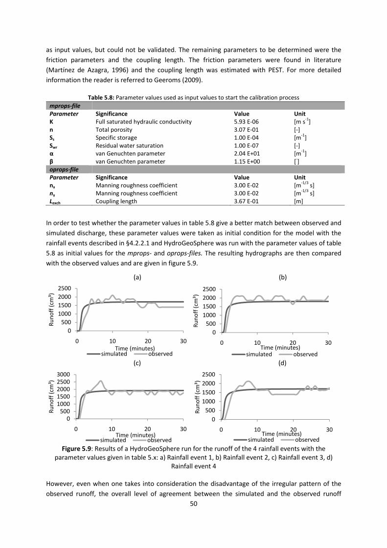
50
as input values, but could not be validated. The remaining parameters to be determined were the
friction parameters and the coupling length. The friction parameters were found in literature
(Martínez de Azagra, 1996) and the coupling length was estimated with PEST. For more detailed
information the reader is referred to Geeroms (2009).
Table 5.8: Parameter values used as input values to start the calibration process
mprops-file
Parameter Significance Value Unit
K Full saturated hydraulic conductivity 5.93 E-06 [m s-1
] n Total porosity 3.07 E-01 [-] Ss Specific storage 1.00 E-04 [m
-1]
Swr Residual water saturation 1.00 E-07 [-] α van Genuchten parameter 2.04 E+01 [m
-1]
β van Genuchten parameter 1.15 E+00 [-]
oprops-file Parameter Significance Value Unit
nx Manning roughness coefficient 3.00 E-02 [m-1/3
s] ny Manning roughness coefficient 3.00 E-02 [m
-1/3 s]
Lexch Coupling length 3.67 E-01 [m]
In order to test whether the parameter values in table 5.8 give a better match between observed and
simulated discharge, these parameter values were taken as initial condition for the model with the
rainfall events described in §4.2.2.1 and HydroGeoSphere was run with the parameter values of table
5.8 as initial values for the mprops- and oprops-files. The resulting hydrographs are then compared
with the observed values and are given in figure 5.9.
(a) (b)
(c) (d)
Figure 5.9: Results of a HydroGeoSphere run for the runoff of the 4 rainfall events with the
parameter values given in table 5.x: a) Rainfall event 1, b) Rainfall event 2, c) Rainfall event 3, d) Rainfall event 4
However, even when one takes into consideration the disadvantage of the irregular pattern of the
observed runoff, the overall level of agreement between the simulated and the observed runoff
0
500
1000
1500
2000
2500
0 10 20 30
Ru
no
ff (
cm³)
Time (minutes)simulated observed
0
500
1000
1500
2000
2500
0 10 20 30
Ru
no
ff (
cm³)
Time (minutes)simulated observed
0500
10001500200025003000
0 10 20 30
Ru
no
ff (
cm³)
Time (minutes)simulated observed
0
500
1000
1500
2000
2500
0 10 20 30
Ru
no
ff (
cm³)
Time (minutes)simulated observed
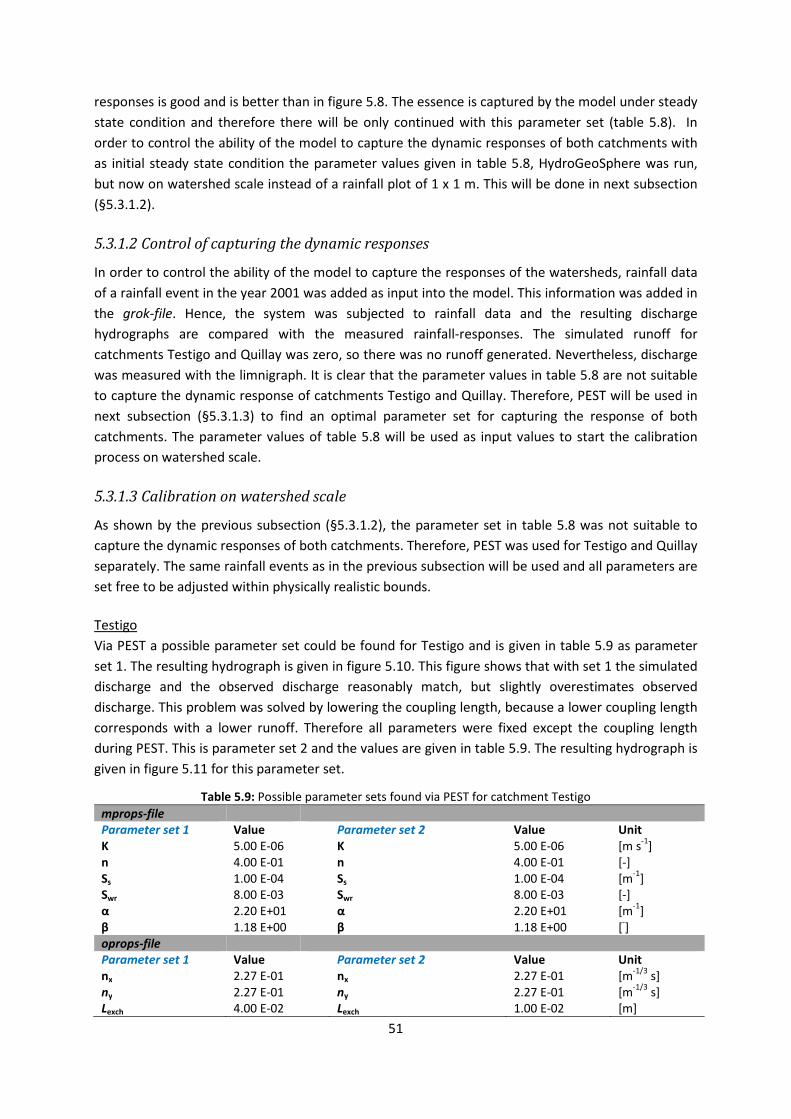
51
responses is good and is better than in figure 5.8. The essence is captured by the model under steady
state condition and therefore there will be only continued with this parameter set (table 5.8). In
order to control the ability of the model to capture the dynamic responses of both catchments with
as initial steady state condition the parameter values given in table 5.8, HydroGeoSphere was run,
but now on watershed scale instead of a rainfall plot of 1 x 1 m. This will be done in next subsection
(§5.3.1.2).
5.3.1.2 Control of capturing the dynamic responses
In order to control the ability of the model to capture the responses of the watersheds, rainfall data
of a rainfall event in the year 2001 was added as input into the model. This information was added in
the grok-file. Hence, the system was subjected to rainfall data and the resulting discharge
hydrographs are compared with the measured rainfall-responses. The simulated runoff for
catchments Testigo and Quillay was zero, so there was no runoff generated. Nevertheless, discharge
was measured with the limnigraph. It is clear that the parameter values in table 5.8 are not suitable
to capture the dynamic response of catchments Testigo and Quillay. Therefore, PEST will be used in
next subsection (§5.3.1.3) to find an optimal parameter set for capturing the response of both
catchments. The parameter values of table 5.8 will be used as input values to start the calibration
process on watershed scale.
5.3.1.3 Calibration on watershed scale
As shown by the previous subsection (§5.3.1.2), the parameter set in table 5.8 was not suitable to
capture the dynamic responses of both catchments. Therefore, PEST was used for Testigo and Quillay
separately. The same rainfall events as in the previous subsection will be used and all parameters are
set free to be adjusted within physically realistic bounds.
Testigo
Via PEST a possible parameter set could be found for Testigo and is given in table 5.9 as parameter
set 1. The resulting hydrograph is given in figure 5.10. This figure shows that with set 1 the simulated
discharge and the observed discharge reasonably match, but slightly overestimates observed
discharge. This problem was solved by lowering the coupling length, because a lower coupling length
corresponds with a lower runoff. Therefore all parameters were fixed except the coupling length
during PEST. This is parameter set 2 and the values are given in table 5.9. The resulting hydrograph is
given in figure 5.11 for this parameter set.
Table 5.9: Possible parameter sets found via PEST for catchment Testigo
mprops-file
Parameter set 1 Value Parameter set 2 Value Unit
K 5.00 E-06 K 5.00 E-06 [m s-1
] n 4.00 E-01 n 4.00 E-01 [-] Ss 1.00 E-04 Ss 1.00 E-04 [m
-1]
Swr 8.00 E-03 Swr 8.00 E-03 [-] α 2.20 E+01 α 2.20 E+01 [m
-1]
β 1.18 E+00 β 1.18 E+00 [-]
oprops-file Parameter set 1 Value Parameter set 2 Value Unit
nx 2.27 E-01 nx 2.27 E-01 [m-1/3
s] ny 2.27 E-01 ny 2.27 E-01 [m
-1/3 s]
Lexch 4.00 E-02 Lexch 1.00 E-02 [m]

52
Figure 5.10: Measured and simulated discharge in Testigo for a rainfall event from 7 until 17 July in
2001 with parameter set 1 as parameter values.
Figure 5.11: Measured and simulated discharge in Testigo for a rainfall event from 7 until 17 July in
2001 with parameter set 2 as parameter values.
Figure 5.11 shows indeed that the discharge is lower than when working with parameter set 1. The
simulated discharge is still higher than the observed runoff but the difference is smaller now. Only
the second simulated runoff peak is now lower than in reality. This suggested that maybe the
coupling length is too low now. Therefore, a manual calibration was performed increasing this
parameter from its initial value of 0.04, with intermediate values of 0.02 m, 0.019 m, 0.018 m, 0.017
m, 0.016 m, 0.015 m, 0.014 m until the best fit was found between the simulated and the observed
discharge. The best fit was found with a coupling length equal to 0.015 m and the resulting
hydrograph is given in figure 5.12. This hydrograph shows good agreement with the hydrograph for
the observations.
0.00E+00
1.00E-06
2.00E-06
3.00E-06
4.00E-06
5.00E-06
6.00E-06
7.00E-06
8.00E-060.00E+00
1.00E-02
2.00E-02
3.00E-02
4.00E-02
5.00E-02
6.00E-02
7.00E-02
8.00E-02
9.00E-02
1.00E-01
16200000 16400000 16600000 16800000 17000000
Pre
cip
itat
ion
(m
s-1
)
Ru
no
ff (
m³
s-1)
Time (s)Observed Simulated Precipitation
0.00E+00
1.00E-06
2.00E-06
3.00E-06
4.00E-06
5.00E-06
6.00E-06
7.00E-06
8.00E-060.00E+00
1.00E-02
2.00E-02
3.00E-02
4.00E-02
5.00E-02
6.00E-02
7.00E-02
8.00E-02
9.00E-02
1.00E-01
16200000 16400000 16600000 16800000 17000000P
reci
pit
atio
n (
m s
-1)
Ru
no
ff (
m³
s-1)
Time (s)Observed Simulated Precipitation

53
Figure 5.12: Measured and simulated discharge in catchment Testigo for a rainfall event from 7 until
17 July 2001 with a coupling length equal to 0.015 m.
In order to make a final decision of which parameter set will be used for evaluating the effect of the
infiltration trenches another rainfall event was used and the resulting hydrographs can be compared.
A rainfall event in the year 1997 was used i.e. the same event as in figure 5.4 (from 3 until 15
October). The hydrograph for parameter set 1 is given in figure 5.13 and the hydrograph for a
coupling length equal to 0.015 m is given in figure 5.14. The best fit according to PEST (parameter set
1) shows again that the simulated discharge and the observed discharge reasonably match. However,
only the simulated runoff is a bit too high compared to the observed runoff. When examining figure
5.14, the runoff is lowered and the match is better. The general features of the measured discharge
are captured with the simulations and the overall level of agreement is good.
Figure 5.13: Measured and simulated discharge in catchment Testigo for a rainfall event from 3 until
15 October in 1997 with parameter set 1 as parameter values.
0.00E+00
1.00E-06
2.00E-06
3.00E-06
4.00E-06
5.00E-06
6.00E-06
7.00E-06
8.00E-060.00E+00
1.00E-02
2.00E-02
3.00E-02
4.00E-02
5.00E-02
6.00E-02
7.00E-02
8.00E-02
9.00E-02
1.00E-01
16200000 16400000 16600000 16800000 17000000
Pre
cip
itat
ion
(m
s-1
)
Ru
no
ff (
m³
s-1)
Time (s)Observed Simulated Precipitation
0
0.000001
0.000002
0.000003
0.000004
0.000005
0.000006
0.000007
0.0000080.00E+00
1.00E-02
2.00E-02
3.00E-02
4.00E-02
5.00E-02
6.00E-02
7.00E-02
8.00E-02
9.00E-02
23700000 23900000 24100000 24300000 24500000 24700000 24900000
Pre
cip
itat
ion
(m
s-1
)
Ru
no
ff (
m³
s-1)
Time (s)Observed Simulated Precipitation
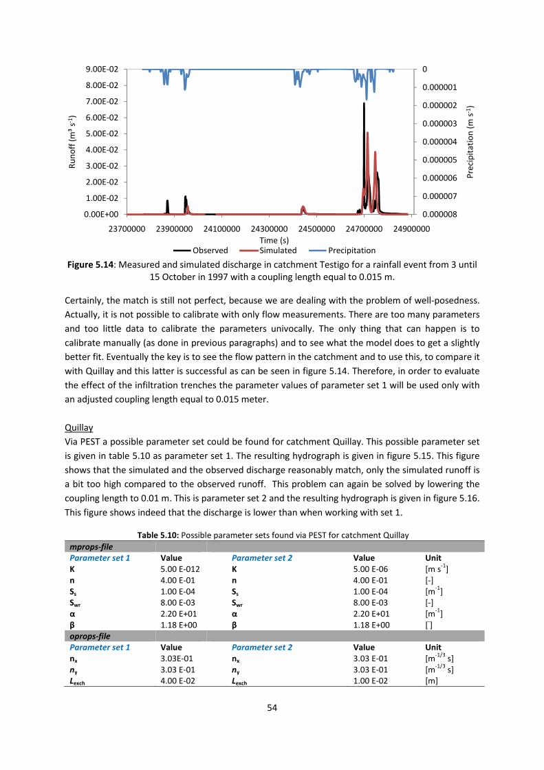
54
Figure 5.14: Measured and simulated discharge in catchment Testigo for a rainfall event from 3 until
15 October in 1997 with a coupling length equal to 0.015 m.
Certainly, the match is still not perfect, because we are dealing with the problem of well-posedness.
Actually, it is not possible to calibrate with only flow measurements. There are too many parameters
and too little data to calibrate the parameters univocally. The only thing that can happen is to
calibrate manually (as done in previous paragraphs) and to see what the model does to get a slightly
better fit. Eventually the key is to see the flow pattern in the catchment and to use this, to compare it
with Quillay and this latter is successful as can be seen in figure 5.14. Therefore, in order to evaluate
the effect of the infiltration trenches the parameter values of parameter set 1 will be used only with
an adjusted coupling length equal to 0.015 meter.
Quillay
Via PEST a possible parameter set could be found for catchment Quillay. This possible parameter set
is given in table 5.10 as parameter set 1. The resulting hydrograph is given in figure 5.15. This figure
shows that the simulated and the observed discharge reasonably match, only the simulated runoff is
a bit too high compared to the observed runoff. This problem can again be solved by lowering the
coupling length to 0.01 m. This is parameter set 2 and the resulting hydrograph is given in figure 5.16.
This figure shows indeed that the discharge is lower than when working with set 1.
Table 5.10: Possible parameter sets found via PEST for catchment Quillay
mprops-file
Parameter set 1 Value Parameter set 2 Value Unit
K 5.00 E-012 K 5.00 E-06 [m s-1
] n 4.00 E-01 n 4.00 E-01 [-] Ss 1.00 E-04 Ss 1.00 E-04 [m
-1]
Swr 8.00 E-03 Swr 8.00 E-03 [-] α 2.20 E+01 α 2.20 E+01 [m
-1]
β 1.18 E+00 β 1.18 E+00 [-]
oprops-file Parameter set 1 Value Parameter set 2 Value Unit
nx 3.03E-01 nx 3.03 E-01 [m-1/3
s] ny 3.03 E-01 ny 3.03 E-01 [m
-1/3 s]
Lexch 4.00 E-02 Lexch 1.00 E-02 [m]
0
0.000001
0.000002
0.000003
0.000004
0.000005
0.000006
0.000007
0.0000080.00E+00
1.00E-02
2.00E-02
3.00E-02
4.00E-02
5.00E-02
6.00E-02
7.00E-02
8.00E-02
9.00E-02
23700000 23900000 24100000 24300000 24500000 24700000 24900000
Pre
cip
itat
ion
(m
s-1
)
Ru
no
ff (
m³
s-1)
Time (s)Observed Simulated Precipitation

55
Figure 5.15: Measured and simulated discharge in Quillay for a rainfall event from 7 until 27 July in 2001
with parameter set 1 as parameter values.
Figure 5.16: Measured and simulated discharge in Quillay for a rainfall event from 7 until 27 July in 2001
with parameter set 2 as parameter values.
In order to make a final decision which parameter set will be used for Quillay, another rainfall event
was used and the resulting hydrographs compared. The same rainfall event as for Testigo was used (3
until 15 October in 1997). The hydrograph for parameter set 1 and 2 is given in figure 5.17.
Figure 5.17: Measured and simulated discharge in Quillay for a rainfall event from 3 until 15 October in
1997 with parameter set 1 and 2 as parameter values.
0.00E+00
1.00E-06
2.00E-06
3.00E-06
4.00E-06
5.00E-06
6.00E-060.00E+00
5.00E-03
1.00E-02
1.50E-02
2.00E-02
2.50E-02
3.00E-02
3.50E-02
4.00E-02
4.50E-02
5.00E-02
16000000 16300000 16600000 16900000 17200000 17500000
Pre
cip
itat
ion
(m
s-1
)
Ru
no
ff (
m³
s-1)
Time (s)Observed Simulated Precipitation
0.00E+00
1.00E-06
2.00E-06
3.00E-06
4.00E-06
5.00E-06
6.00E-060.00E+00
5.00E-03
1.00E-02
1.50E-02
2.00E-02
2.50E-02
3.00E-02
16250000 16550000 16850000 17150000 17450000
Pre
cip
itat
ion
(m
s-1
)
Ru
no
ff (
m³
s-1)
Time (s)Observed Simulated Precipitation
0.00E+00
1.00E-06
2.00E-06
3.00E-06
4.00E-06
5.00E-06
6.00E-06
7.00E-06
8.00E-060.00E+00
5.00E-03
1.00E-02
1.50E-02
2.00E-02
23700000 23900000 24100000 24300000 24500000 24700000 24900000
Pre
cip
itat
ion
(m
s-1
)
Ru
no
ff (
m³
s-1)
Time (s)
Simulated with parameter set 1 Simulated with parameter set 2 Observed Precipitation

56
Figure 5.17 shows that with parameter set 2 the dynamic response was not always captured and this
in contrast with parameter set 1. With parameter set 1 the simulated discharge was sometimes
higher than the observed runoff (like in figure 5.15) but the general features were captured and this
is the most important factor. Therefore, in order to evaluate the effect of the infiltration trenches the
parameter values of parameter set 1 will be used for catchment Quillay.
5.3.2 Evaluation of the infiltration trenches based upon modeling
Since model calibration is achieved in the previous subsection (§5.3.1.3), the model can be used to
predict the effect of the infiltration trenches by comparing the simulated discharge hydrograph of
Testigo with the discharge hydrograph of Quillay. First, rainfall data of the whole year 2001 was used
to model the effect of the trenches and the corresponding hydrographs of Testigo and Quillay are
given in figure 5.18a. This simulation was done with the finest and the most representative grids, as
shown earlier in figure 4.3 and 4.4. From figure 5.18a convincing evidence was found that the
furrows have an effect on reducing peak runoff. The simulation in Testigo and Quillay indicated that
the infiltration trenches can effectively be used to buffer excess rainfall and thus will lead to reduced
soil losses. The corresponding observed discharge in Quillay and Testigo is given in figure 5.18b.
Figure 5.18: Comparison between the discharge in Quillay and Testigo in 2001: a) based on
simulations on fine grids, b) based on observations. The corresponding precipitation is also given.

57
Figure 5.18b is the same as figure 5.1 but now expressed in different units. This was done in order to
obtain a comparison with the simulations. As mentioned in §5.1 the limnigraph did not work in the
beginning of the rainfall event in both catchments and also did not work in catchment Quillay at the
end of the rainfall event (from 20463600 s). If we compare figure 5.18a and 5.18b, it is clear that the
general features of the measured discharge are captured with the simulations. Figure 5.18b shows
also that the discharge peaks in Quillay are lower than in Testigo and that the rainfall is effectively
buffered by the trenches. Except at the end of the rainfall event the peak is higher in the watershed
with the measurements due to a delay in runoff travel time in the trenches.
The same rainfall event can be used but now evapotranspiration data will be added to the model. In
this way the simulation is closer to reality. The calibration process in (§5.3.1) was done without
evapotranspiration data, because otherwise too many parameters needed to be calibrated with little
data. The corresponding hydrographs for Quillay are given in figure 5.19 and those for Testigo in
figure 5.20. Adding evapotranspiration to the model should, in theory, make the model more realistic
and therefore the simulated runoff should match the observed discharge better. In figure 5.19, it is
shown that in the beginning the simulation with evapotranspiration (ET) data matches more with the
observations than the simulation without ET data. However, this is not always the case as can be
seen in the right part of the figure.
Figure 5.19: Comparison between discharge in Quillay in 2001 when the simulation is based on the finest grids with and without evapotranspiration data.
In Figure 5.20, it is shown that the discharge is indeed lowered to match more the observed values
but it is too much lowered in most of the cases and therefore the match between observed and
simulated is still not good enough. In general, both in Testigo and Quillay the simulations with ET
data gave no better match between the observations and simulations than the simulations without
ET data. This is possible due to the fact that not all the input values were known in literature and an

approximation was taken for the values
the input values for introducing evapotranspiration in the model would improve the results.
Figure 5.20: Comparison between discharge in Testigo in 2001 when the simulation is based on the finest grids with and without evapotranspiration data.
A similar simulation was done but now on the coarse grids, as shown in figure
two different grid configurations can be compared. The fine grids allow a more realistic description of
the local phenomenon at the river zone. The most realistic simulation (fine
one with the best match between observed and simulated.
the coarse grids are given in figure 5.21 for Quillay and in figure 5.22 for Testigo
Figure 5.21: Discharge in Quillay in 2001 w
0.00E+00
2.00E-02
4.00E-02
6.00E-02
8.00E-02
1.00E-01
1.20E-01
1.40E-01
1.60E-01
1.80E-01
2.00E-01
11000000 13000000
Ru
no
ff (
m³
s-1)
Simulated without ET data
58
approximation was taken for the values. Therefore, it is expected that a more rigorous description of
evapotranspiration in the model would improve the results.
Comparison between discharge in Testigo in 2001 when the simulation is based on the finest grids with and without evapotranspiration data.
done but now on the coarse grids, as shown in figure 4.5
two different grid configurations can be compared. The fine grids allow a more realistic description of
the local phenomenon at the river zone. The most realistic simulation (fine grid) is expected to be the
one with the best match between observed and simulated. The hydrographs of the simulations with
e grids are given in figure 5.21 for Quillay and in figure 5.22 for Testigo.
in Quillay in 2001 when the simulation is based on the finest
13000000 15000000 17000000Time (s)
Simulated without ET data Observed Simulated with ET data
Therefore, it is expected that a more rigorous description of
evapotranspiration in the model would improve the results.
Comparison between discharge in Testigo in 2001 when the simulation is based on the
4.5 and 4.6. As such,
two different grid configurations can be compared. The fine grids allow a more realistic description of
grid) is expected to be the
The hydrographs of the simulations with
.
tion is based on the finest and coarse grid
17000000 19000000
Simulated with ET data

59
Figure 5.22: Discharge in Testigo in 2001 when the simulation is based on the finest and coarse grid
In Quillay the simulation based on a coarse grid overestimates the runoff. This is due to the fact that
when a coarse grid is used the trenches are not incorporated well in the grid and therefore the
furrows will retain less rainfall. In Testigo the simulation based on a coarse grid underestimates the
runoff considerably. This is due to the fact that the river was not incorporated well in the grid
because of its coarseness and therefore less runoff is predicted. It is clear that the simulations with
the fine grids matches better the observed discharges than the coarse grids. The theoretic
assumption that the fine grid will give the best fit is therefore confirmed.
Finally, to evaluate the efficiency of the infiltration furrows in terms of runoff, the total simulated
runoff in watershed Testigo can be compared with the results from the total runoff simulated in
Quillay for different years. A dry year (year 1998), a wet year (year 2000) and a normal year namely
the year 2001 will be used. The results from the runoff simulations are given in table 5.11.
Table 5.11: Runoff values for simulations of a normal, wet and dry year
Normal year 2001 Wet year 2000 Dry year 1998
Precipitation (mm) 438 893 144 With infiltration furrows (m³) 15505 57422 1381 Without infiltration furrows (m³) 17995 74303 1642 Percentage runoff withhold 14% 23% 16%
From table 5.11 it is clear that the infiltration furrows were not able to withhold all the runoff. But
the trenches have an important influence on runoff amounts, with reductions in percentage runoff
withhold for three years. Despite the reduction in runoff the amounts of runoff withhold will not be
enough to ensure a sufficient erosion control. The results indicate that infiltration furrows can
effectively be used to buffer excess rainfall from semi-arid hillslopes during low intensity rain events
and will thus lead to reduced erosion and reduced land degradation hazards (as mentioned in the
literature review in §3.5). The effectiveness reduces however due to trench overfilling when rainfall
intensities and amounts increase. Therefore, the infiltration trenches must be optimally designed for
the soil physical and climatic conditions available at Alto Loica.
0.00E+00
2.00E-02
4.00E-02
6.00E-02
8.00E-02
1.00E-01
1.20E-01
1.40E-01
1.60E-01
1.80E-01
2.00E-01
11000000 13000000 15000000 17000000 19000000
Ru
no
ff (
m³
s-1)
Time (s)Simulated fine grid Observed Simulated coarse grid

60
Chapter 6
Conclusion and discussion Soil erosion is an important hazard in Chile and this leads to land degradation resulting in less water
infiltrating in the soil and less water available for plant production. Water harvesting techniques are
a potential solution to this problem. Water harvesting techniques were developed centuries ago and
although various water harvesting techniques are realized, few efforts are made to quantify the
effect of these techniques. Therefore the objective of this study was the use of HydroGeoSphere, a
fully coupled model, for the evaluation of the infiltration furrows on the river discharge in a semi-arid
zone of Chile.
The study was performed in Alto Loica, a small village located in the metropolitan region in the
province of Melipilla and the community of San Pedro. In this village, a number of soil conservation
techniques, such as infiltration trenches, were installed in three micro-basins in the scope of a
project on erosion control. In this study, two watersheds are compared, one with soil conservation
techniques installed, called Quillay, and a second one, Testigo, which represents a natural,
unchanged watershed. Input data was gathered in Quillay and Testigo and this included the hydraulic
conductivity from tension disk infiltrometry and Guelph permeameter measurements. Furthermore
undisturbed soil samples were taken to determine the soil water retention curve. The design of the
infiltration furrows and the characteristics of the catchments were carefully measured in order to
construct grids that were representative for the real situation.
6.1 Evaluation of infiltration trenches applied in Quillay
The use of the implemented infiltration trenches in Quillay was evaluated by comparing both
catchments. This comparison was done via three ways: i) by comparing measurements of the rainfall
and discharge obtained by CONAF and JICA, ii) by comparing soil physical properties in both
catchments and iii) by comparing via modeling.
6.1.1 Evaluation of infiltration furrows via rainfall and discharge measurements
This evaluation was based on the comparison of the discharge of Testigo with the discharge of
Quillay for given rainfall events. The problem with this starting point is two-sided. There is a
difference in size between Testigo and Quillay. Small differences in peak runoff can therefore be the
result of the size difference between the two catchments. But the clearly larger differences can be
explained as the effect of the infiltration furrows. A second point is that a large range of treatments
were introduced in Quillay, including the infiltration furrows. Therefore, it is possible that the effect

61
of a reduction in peak runoff is the result of not only the infiltration furrows. Nevertheless, the
infiltration furrows were the main treatment, therefore it can be expected that the effect of
reduction in peak runoff is mainly due the infiltration trenches.
The evaluation of the discharge measurements was done for rainfall events in three years, namely
2001 (normal year), 1998 (dry year) and 1997 (wet year). In 2001, lower discharge peaks were
observed in Quillay and when the discharge was expressed on a logarithmic scale a delay in runoff
travel time due to the infiltration trenches could be seen clearly. In the dry year no runoff was
observed in Quillay in contrast with Testigo where discharge was measured. So, the precipitation was
stored in Quillay and therefore increased the plant available water in a dry year. Also in the wet year
convincing evidence was found that the infiltration furrows have an effect in reducing peak runoff
(more than a half of the values that were observed in Testigo). Finally, a second rain event in the
same year was used. In this rain event a lot of precipitation peaks had followed each other quickly
and saturated the soil. Even at this moment the infiltration furrows were able to reduce the runoff
peak with more than a half of the value that is observed in Testigo. But this was not always the case.
At the end of a long rainfall event (the whole year of 2001) the peak was higher in the watershed
with the measurements due to a delay in runoff travel time in the trenches.
The idea is suggested that the measurements are able to withhold a big part of the total amounts of
precipitation, but not the total amount. This is due to under-dimensioning of the infiltration furrows.
These findings illustrate the importance of the dimensions of the infiltration furrow system and the
importance to look for better dimensions to optimize this erosion control system.
6.1.2 Evaluation of infiltration furrows via field measurements
First, field measurements of the hydraulic conductivity were done via the Guelph permeameter. No
statistic differences were found between the log(Kfs) of the two catchments. This suggests that the
soil conservation measures, such as the infiltration furrows, had not impacted the soil properties
sufficiently to observe any measurable differences. This confirms the results of Daelman (2009), who
didn’t find any significant differences when using a tension infiltrometer. No significant difference
was observed between the log (kfs) resulted from measurements located in the western and the
eastern part of the watershed. Finally also no significant difference was found between the log (kfs) of
the three transects in each watershed. However, a same trend was observed in Testigo and Quillay,
namely the log(Kfs) of the western part of the watersheds and the log(Kfs) of transect 3 in each
catchment was higher than respectively the eastern part and the other transects.
Field measurements were also done with the tension disk infiltrometry. A two-sample independent
T-test was used to investigate if there was a significant difference between the Kh of Testigo and
Quillay. All the two-sample independent T-tests indicated that there was a significant difference
between the hydraulic conductivities of Testigo and Quillay. The T-test was also used to compare the
values of Quillay obtained this year with the values of Quillay obtained in 2009. Also here the T-test
indicated a significant difference. Based on current knowledge, no clear reason could be found that
explains the measured differences between both data sets.
Finally, soil samples were taken at a depth of 35 cm to determine the soil water retention curves.
From the soil-water retention curve, the available water capacity �ÑÒ� [m³ m-3] was estimated for

62
both catchments and for each transect within each watershed. No significant difference was found
between the �ÑÒ� of the two catchments. Also, no significant differences were found between the
transects in each watershed. Soil samples were already taken at a depth of 5 cm in an earlier study
and also here no significant difference was found between �ÑÒ� inside and outside the trench. This
shows the homogeneous conditions occurring in both catchments, allowing them to be considered
equal in terms of their hydrophysical properties.
6.1.3 Evaluation of infiltration furrows via modeling
In the third kind of evaluation HydroGeoSphere was introduced to model the effect of the infiltration
furrows. PEST was used to find an optimal parameter set to use as initial condition. The main
problem that was encountered was that the parameter sets found with PEST gave still no perfect
match between observed and simulated runoff. This was because we are dealing with the problem of
well-posedness. It was not possible to calibrate all model parameters with only flow measurements.
There are too many parameters and too little data to calibrate the parameters univocally. Therefore,
manual calibration was required to calibrate further. The final objective consists of visualizing the
flow pattern in the catchment and to use this to compare the two watersheds.
The simulation with fine grids in Testigo and Quillay indicated that the infiltration trenches can
effectively be used to buffer excess rainfall and thus will lead to reduced soil losses and reduced land
degradation hazards (as mentioned in the literature review). After comparing the simulations with
the observations, it turned out that the general features of the measured discharge are captured
with the simulations with fine grids. When evapotranspiration data was added to the model it was
expected that simulated and observed runoff would match better. Unfortunately this was not always
the case. A more rigorous description of the input values for introducing evapotranspiration in the
model would improve the results. Therefore it is important that further research is done to update
the input values to the most realistic and correct ones. At the end two different grid configurations
(coarse and fine) were compared. The theoretic assumption that the fine grids will give a better fit
between observed and simulated discharge, due to the more realistic description of the local
phenomenon at the river zone and the infiltration trenches, was confirmed with the simulations.
Finally, in order to evaluate the efficiency of the infiltration furrows in terms of runoff, the total
simulated runoff in Testigo was compared with the results from the total simulated runoff in Quillay
for a dry year, normal year and a wet year. The trenches had an influence on runoff amounts, but not
enough to ensure a sufficient erosion control. Therefore the infiltration trenches must be optimally
designed for the soil physical and climatic conditions available at Alto Loica and further research into
the dimensions of the trenches, other than those mentioned in the literature review (§3.5), will teach
us much more about the optimal design of the trenches.
6.2 Problems and possibilities related to HydroGeoSphere
6.2.1 Problems
HydroGeoSphere is a coupled model and therefore a coupling between the surface and subsurface
flow needs to be accomplished. The coupling is done by inserting a (none visualized) thin layer of
porous material between the two domains across where water exchange will occur. The layer is very

63
important in regulating the flux between both domains but the thickness of this non-existing layer
has to be introduced as an input into the models. The problem with the coupling length is the great
influence it has on the outcome of the models as shown in chapter 5 (§5.3.1.3), but since the layer is
nonexistent it cannot be measured. The only way to define the parameter is by means of inverse
modeling. This was tried in this study by using only runoff data, but as mentioned before no perfect
match was found, because there were only flow measurements available for calibration. A solution
for this problem is to use different types of observations, preferably spread over both domains, e.g.
soil moisture data combined with runoff data. This was the original position in this study by using
runoff data generated by a rainfall simulator, in combination with measurements of the evolution in
soil moisture content by means of TDR-probes. Unfortunately the TDR data set was not suitable for
calibration. The coupling length will play a decisive role in determining whether or not fully coupled
models can be used for future investigation of this type. It is important that further research is done
on possible other ways of coupling or on an improved knowledge about the coupling length.
A second problem is the fact that high demands were posed to the computer system, e.g. the PEST
run of catchment Quillay took more than 2 weeks (day and night) to complete. It is also different
when more detailed grids and heavier grids are used, e.g. a HydroGeoSphere run of catchment
Testigo (less heavy grid than catchment Quillay) took approximately one hour and a run of Quillay
took more than 12 hours. Therefore, high computer standards are to be obtained when larger or
more detailed grids are used as an input to handle the heavier grids. This problem will probably solve
itself when faster and more affordable computers are developed, and when parallel versions become
available.
Finally, another problem related to HydroGeoSphere is that is still rather new and can still contain
some bugs. During this study bugs were encountered from time to time which often had to do with
the large scale of the grids, but it has to be noticed that the developers of the software were very
helpful and were always available to solve these problems.
6.2.2 Opportunities
Despite the above problems and limitations, the HydroGeoSphere software package offers a lot of
new opportunities. The first opportunity is that HydroGeoSphere belongs to the second generation
of fully-integrated numerical models that take into account all components of the hydrologic cycle
and simultaneously solves the governing equations for the surface and subsurface domains. This
offers great opportunities in modeling soil-water systems as shown in this study.
A second opportunity the model offers is the one for designing grids. As shown in this study also
designing large scale grids belongs to the abilities. The design of the grids can also easily be
manipulated which allows the use of HydroGeoSphere for evaluating other types of systems.
Overall it is concluded that the model is capable of simulating fully-integrated surface-subsurface
flow processes at catchment scale. Moreover I believe that this fully-integrated approach to
watershed simulation and analysis has the potential to greatly improve upon existing conventional
approaches that either consider surface and subsurface processes separately or link them together in
a weakly coupled manner. Therefore further research on the bottlenecks is needed.

64
Chapter 7
Nederlandse samenvatting
(Summary in Dutch)
7.1 Inleiding
Erosie is het proces waarbij slijtage van een vast oppervlak optreedt en waarbij materiaal wordt
verplaatst of geheel verdwijnt. Erosie gebeurt vooral via wind en water, maar watererosie is het
meest belangrijke landbouwkundig probleem in Chili. Circa 25.4% van het continentale Chili is aan
erosie onderhevig en de erosie is van invloed op meer dan 60% van de totale bruikbare grond (Ellies,
2000). Watercaptatietechnieken zoals de infiltratiegreppels worden vaak toegepast om de infiltratie
in de bodem te verhogen. Het zijn ook erosiebestrijdingsmaatregelen om landdegradatie te
verminderen (Verbist et al., 2009). Verschillende projecten betreffende dit aspect werden al
gerealiseerd (CONAF and JICA, 1998), maar er zijn nog maar weinig inspanningen gedaan om het
effect van watercaptatietechnieken te kwantificeren. Daarom wordt in deze thesis het effect van de
infiltratiegreppels op de rivier afstroming in Chili onderzocht. Een combinatie van gedetailleerde
veldmetingen en modellering met het HydroGeoSphere software pakket werd gebruikt om het effect
van de infiltratiegreppels te visualiseren. Dit werd gedaan door de evaluatie van de beschikbare
meetgegevens tijdens de samenwerking tussen CONAF (Chileense nationale dienst voor
bosbouw) en JICA (Japanse internationaal coöperatief agentschap) en het gebruiken van deze
gegevens om het hydrologische 3D-model te kalibreren.
Een korte algemene beschrijving van Chili en het studiegebied Alto Loica zal gegeven worden in §7.2.
Het tweede deel (§7.3) bestaat uit een literatuuronderzoek over landdegradatie en erosie. In het
derde deel (§7.4) zullen de materialen en de methoden die toegepast werden gedurende de thesis
worden toegelicht. In het vierde deel (§7.5) wordt de eigenlijke evaluatie doorgevoerd van het effect
van de infiltratiegreppels. In het laatste stuk (§7.6) worden de conclusies gegeven.
7.2 Beschrijving van het studiegebied
7.2.1 Chili
De Republiek Chili is een lang en smal land in Zuid-Amerika. Chili heeft een gemiddelde breedte van
177 km en is 4270 km lang (LOC, 2010). Het wordt begrensd door de Andes in het oosten en de Stille

65
oceaan in het westen. Chili is sinds 2007 verdeeld in 15 administratieve regio’s (CONAF, 2010).
Chili heeft een zeer uiteenlopend geografisch karakter. Het varieert van noord naar zuid en van west
naar oost. Het noorden wordt gekenmerkt door één van de droogste woestijnen, namelijk de
Atacama woestijn. Het zuiden echter is rijk aan bossen, graslanden, meren en vulkanen (U.S.
Department of State, 2010). In Chili is het klimaat zo divers als de geografie en dit aspect zorgt ervoor
dat veralgemeningen moeilijk te maken zijn.
7.2.2 Alto Loica
Alto Loica is gelegen in de hoofdstedelijke regio, in de provincie Melipilla en de gemeenschap van San
Pedro. Het alto Loica project is gelegen dicht bij de grens van de 6de regio en is 77.12 hectare groot.
Het gebied bestaat uit milde heuvels van 200 tot 350 meter hoogte. De hellingen van deze heuvels
variëren van 5 tot 15 graden. Oppervlakte-erosie kan waargenomen worden in 63% van het gebied
en ravijnerosie voor 24% (Fujieda and Vargas, 2005).
Het klimaat staat bekend als een mediterraan klimaat met neerslag in de winter (Tokugawa and
Vargas, 1996). De gemiddelde jaarlijkse neerslag voor de periode 1961 – 1991 was 398.5 mm met
een standaarddeviatie van 139.8 mm. Circa 88% van de jaarlijkse regenval vond plaats van mei tot
september. De maximum temperatuur bedroeg 32.2 graden in januari en de minimale temperatuur
was 3.4 graden in juli (Fujieda and Vargas, 2005). Het mediterrane klimaat is een klimaat waarin
regenval in de winter drie keer groter is als in de zomer. Dit sterk contrast resulteert in een
uitdroging van de bodem tijdens de zomer, vaak voor enkele maanden (Yaalon, 1997). De wind is ook
een factor die een belangrijke rol speelt in de droogte van de regio. De wind waait in de herfst van 11
uur tot 8 uur in zuidoostelijke richting en de gemiddelde snelheid is 4 m s-1, maar kan oplopen tot
10 – 12 m s-1 (CONAF and JICA, 1995).
7.3 Literatuurstudie
7.3.1 Landdegradatie en oppervlakkige afstroming
Landdegradatie bestaat uit de verslechtering van de bodemkwaliteit en de vegetatie. Degradatie van
de bodem zal de productiecapaciteit van de bodem verminderen. Landdegradatie begint met de
verdwijning van de natuurlijke vegetatie en de bodem is daardoor onderworpen aan directe
zonnestraling en overmatige oxydatie. Dit veroorzaakt de dood van levende organismen en een
versnelling van de biodegradatie van de humus, waardoor aggregaten verdwijnen en de porositeit
daalt. Hierdoor kunnen water en lucht niet gemakkelijk meer circuleren en het oppervlak wordt
gecompacteerd en kan zelfs impermeabel worden. Bijgevolg kan neerslag afstromen in plaats van
opgeslagen te worden (Gualterio, 2006).
Als het regent, worden de eerste druppels onderschept door de bladeren en de stengels. Als de
regen aanhoudt, infiltreert het in de bodem tot de neerslagintensiteit groter wordt dan de
infiltratiecapaciteit. Depressies zijn dan gevuld. Daarna wordt afstroming gegenereerd. Deze duurt
zolang de neerslagintensiteit groter is dan de werkelijke infiltratiecapaciteit, maar stopt als de
snelheid van de regenval daalt tot minder dan de werkelijke snelheid van infiltratie (Critchley et
al., 1991). Oppervlakkige afstroming veroorzaakt erosie en deze is vaak van grote omvang en

66
onomkeerbaar. Als de afstroming georganiseerd wordt in kleine groeven, zal de snelheid en de
kinetische energie verhogen. Dit levert voren of groeven. Tot slot kunnen er geulen ontwikkeld
worden met als resultaat een totaal verlies van de bodem. Erosie leidt tot landdegradatie wat
resulteert in een verstoring van het natuurlijk bodemevenwicht, een lagere infiltratie van water en
minder water beschikbaar voor de productie van planten. Er ontstaat ook een toenemende mate van
afstroming en dit zorgt voor een intensificatie van het erosieproces. Ongeveer 60% van de bos- en
agrarische gebieden in Chili vertonen matige tot zeer ernstige erosie (Soto, 1999).
De topografische toestand en regenvalkenmerken zoals frequentie, intensiteit en duur zijn factoren
die een rol spelen in het afstromingsproces. Eveneens is het origineel materiaal van de bodem
bepalend. Tenslotte speelt de vegetatiebedekking een rol, want dichte begroeiing schermt de bodem
van de impact van de regendruppels. Ontbossing leidt tot meer erosie, omdat de impact afkomstig
van de energie uit de regendruppels op de bodem wordt verhoogd. Daarom zijn bebossingsprojecten
zeer belangrijk. Bovendien zorgt het wortelsysteem voor een verhoogde porositeit en meer
infiltratie. Vegetatie vertraagt ook de oppervlakkige afstroming, waardoor het water meer tijd heeft
om te infiltreren (Critchley et al., 1991).
7.3.2 Watercaptatietechnieken
7.3.2.1 Classificatie
Terwijl irrigatie de meest voor de hand liggende reactie is op droogte, is het zeer duur. Het is ook
gebaseerd op geavanceerde technologie, die meestal ontbreekt in de meeste semi-aride gebieden. Er
is nu een toenemende belangstelling in een goedkoop alternatief, namelijk watercaptatietechnieken.
Hierbij wordt de afstroming opgevangen en opgeslagen. Hierdoor wordt de infiltratie in de bodem
verhoogd en is het water weer beschikbaar voor plantaardige productie. Watercaptatietechnieken
kunnen worden beschouwd als een rudimentaire vorm van irrigatie. Het verschil is dat met
watercaptatietechnieken de landbouwer er weinig controle over heeft. Water kan alleen worden
verzameld wanneer het regent. De beschikbare regen kan echter worden geconcentreerd op een
kleiner gebied, zodat toch een redelijke opbrengst bereikt wordt. Natuurlijk zal in een jaar van
ernstige droogte niet veel afstroming verzameld worden, maar een efficiënte watercaptatietechniek
zal de groei van de planten meestal verbeteren (Critchley et al., 1991). Bij watercaptatietechnieken
wordt afstroming van regen verzameld door de koppeling van een afstromingsgenererend gebied
aan een afstromingsontvangend gebied. De technieken worden meestal ingedeeld in drie
categorieën op basis van de grootte van het ontvangende gebied, namelijk in situ
watercaptatietechnieken, micro-stroomgebied systeem en een macro-stroomgebied systeem.
Bij in situ technieken wordt de neerslag opgevangen waar het valt. Het is eigenlijk de preventie van
netto afvoer van een bepaalde beteelde oppervlakte door de neerslag te weerhouden en op deze
manier de tijd voor infiltratie te verhogen.
Bij het micro-stroomgebied systeem is er een duidelijke scheiding tussen een afstromingsgenererend
stroomgebied en een gecultiveerd bekken waar de afstroming wordt opgeslagen in de wortelzone en
productief gebruikt wordt door planten. Het genererende gebied en het bekken bevinden zich naast
elkaar (Mbilinyu et al., 2005). Het genererende gebied is meestal tussen de één en 30 meter lang en
de verhouding tussen het genererende en het ontvangende gebied is normaal tussen 1:1 en 1:3.

67
Het macro-stroomgebied systeem wordt echter gekenmerkt door afstroming van neerslag van
relatief grote stroomgebieden (30 tot 200 meter lang) en de ratio tussen het genererende en het
ontvangende gebied is tussen 2:1 en 10:1. Hoe groter de omvang van het generend stroomgebied
hoe groter de afstand de afstroming van neerslag moet overtreffen en hoe lager het percentage
verzamelde afstroming. De kleinere stroomgebieden (micro-stroomgebieden) hebben dus een
hogere afstromingsefficiëntie (volume afstroming per oppervlakte-eenheid). Dit is een groot
voordeel van micro-stroomgebieden (Critchley et al., 1991).
7.3.2.2 Infiltratiegreppels
Het infiltratiegreppel systeem is een micro-stroomgebied systeem met als belangrijkste
doelstellingen (CONAF and JICA, 1998b):
• Recuperatie van de bodem door het opvangen van de afstroming van neerslag op hellingen.
Op deze manier wordt erosie voorkomen.
• Het verhogen van de infiltratie van neerslag in de bodem.
• Verlaging van de oppervlakkige afstroming en zijn snelheid.
Het is duidelijk dat de infiltratiegreppels een goed hulpmiddel zijn om landdegradatie te verminderen
doordat meer water infiltreert. Daardoor is er ook meer water beschikbaar voor plantaardige
productie. Dit verhoogt de overlevingskansen van nieuwe geïntroduceerde planten. De
infiltratiegreppel is een niet-hellend kanaal dat uitgegraven wordt in een helling. Dit wordt loodrecht
gedaan op de richting van de helling en is evenwijdig aan de contourlijnen. Onderstaande
specificaties van de infiltratiegreppels worden aanbevolen door CONAF en JICA (CONAF and JICA,
1998b). Wat tussen haakjes staat, is wat toegepast werd in Quillay.
• Een breedte aan de top tussen de 0.52 en 1 meter (0.52 meter)
• Een breedte aan de voet van 0.2 meter (0.2 meter)
• Een diepte tussen de 0.2 en 0.4 meter (0.2 meter)
• Een lengte tussen de 2.5 en 5 meter (variërend)
De implementatie van de infiltratiegreppels is sterk toegenomen in de aride en semi-aride gebieden
in Chili, namelijk van 52 hectare in 2001 tot 2200 hectare in 2003. Dit is te wijten aan sterk prikkels
(Pizarro et al., 2004). Om een geschikt erosiebestrijdingssysteem te behalen werden drie
microbekkens opgezet in de sector van Alto Loica (CONAF and JICA, 1995). In deze microbekkens
werden watercaptatietechnieken geconstrueerd zoals de infiltratiegreppels. Microbekken 2 is Quillay
en naast Quillay is er een tweede soortgelijk stroomgebied, genaamd Testigo. In beide
stroomgebieden was een limnigraph geïnstalleerd om de afstroming te meten en een pluviometer
om de hoeveelheid neerslag te meten op een dagelijkse basis (CONAF and JICA, 1998). In deze thesis
werd enkel het brongebied van beide stroomgebieden bestudeerd. Het brongebied van Quillay is
2.88 hectare groot en die van Testigo is 3.60 hectare. Desondanks er al veel watercaptatietechnieken
zijn aangelegd, zijn er nog maar weinig pogingen gedaan om het effect te kwantificeren van de
infiltratiegreppels op de rivier afstroming. Aangezien er in Testigo geen watercaptatietechnieken
werden geïmplementeerd, kan er een vergelijkende studie uitgevoerd worden tussen de
stroomgebieden om zo het effect na te gaan van de infiltratiegreppels. Een combinatie van
gedetailleerde veldmetingen en modellering met het HydroGeoSphere software pakket werd
gebruikt om het effect te visualiseren. Dit wordt toegelicht in het volgende hoofdstuk.

68
7.4 Materiaal en methode
In §7.4.1 zal de HydroGeoSphere software worden uitgelegd dat gebruikt werd om het effect van de
infiltratiegreppels te visualiseren. Vooraleer het te gebruiken voor de effect evaluatie, moet het
model eerst gekalibreerd worden. Hiervoor zal PEST gebruikt worden en hoe dit werkt, wordt
uitgelegd in §7.4.2. De effect evaluatie gebeurt niet alleen via HydroGeoSphere, maar ook via
veldmetingen. Dit laatste wordt uitgelegd in §7.4.3.
7.4.1 HydroGeoSphere
Modellen voor watertransport over het oppervlak en in de ondergrond zijn een nuttig hulpmiddel
voor het begrijpen van fysische processen en voor het valideren van wetenschappelijke hypothesen.
Oppervlakte en ondergrondse waterstromingsmodellen kunnen opgedeeld worden in drie klassen:
de ongekoppelde, de iteratief gekoppelde en de volledig gekoppelde modellen. Voorbeelden van
volledig gekoppelde modellen zijn InHM (Vanderkwaak, 1999), ParFlow (Kollet and Maxwell, 2006)
en HydroGeoSphere (Therrien et al., 2010). Deze modellen houden rekening met alle componenten
van de hydrologische cyclus en de vergelijkingen van de bovengrondse en ondergrondse domeinen
worden tegelijk opgelost. Dit is in schril contrast met de vorige generatie van modellen waarbij de
vergelijkingen afzonderlijk werden opgelost voor elk domein en uiteindelijk werden geassembleerd
via iteratie (Sciuto and Diekkrüger, 2010).
Het model dat in deze masterproef gebruikt wordt is het geïntegreerde driedimensionale
oppervlakte-ondergrond model HydroGeoSphere. Het is een krachtige numerieke simulator dat
reeds succesvol is toegepast op een groot aantal schalen, van relatief kleine deelstroomgebieden,
bijvoorbeeld Sudicky et al. (2008), tot grotere stroomgebieden, bijvoorbeeld Li et al. (2008).
Naarmate de schaal vergroot zal ook de rekentijd toenemen. HydroGeoSphere heeft duidelijk het
potentieel voor kleine en grootschalige hydrologische studies en dit zal nog meer toenemen in de
toekomst, aangezien de rekenkracht van computers steeds sterker wordt en deze computers ook
steeds meer betaalbaar worden.
In de volgende paragrafen wordt een kort overzicht gegeven van de belangrijkste processen van de
HydroGeoSphere software die gebruikt werd in deze thesis. Ook een pre-processor genaamd Grid
builder werd gebruikt om de ‘grids’ van de stroomgebieden Testigo en Quillay te genereren. In de
laatste paragraaf worden de nodige input en output bestanden besproken.
7.4.1.1 Belangrijkste processen
Er zijn drie fluxen die optreden, namelijk een oppervlakte, een ondergrondse en een interface flux.
De simulaties berekenen de fluxen in elk van deze drie onderdelen op het zelfde moment, waardoor
een geïntegreerd model wordt bekomen. Waterstroming in het poreuze medium wordt gesimuleerd
in drie dimensies met behulp van de Richards vergelijking voor variabele verzadigde ondergrondse
stromingen. De oppervlakte stroming wordt gesimuleerd met behulp van de tweedimensionale Saint
Venant vergelijkingen. De ondergrond en het oppervlak zijn complexe systemen die zich vaak in een
gekoppelde manier gedragen. Vanwege dit feit hebben volledig gekoppelde modellen zoals
HydroGeoSphere een groot voordeel, namelijk een volledige koppeling tussen de oppervlakte en de

69
ondergrondse stroming. De water uitwisseling tussen de twee domeinen wordt gedefinieerd aan de
hand van een Darcy flux. De flux wordt berekend aan de hand van het verschil in hydraulische hoogte
tussen de twee domeinen. Het veronderstelt ook dat de twee domeinen van elkaar gescheiden zijn
door een (niet zichtbare) dunne laag van poreus materiaal waarover de wateruitwisseling zal
optreden (Therrien et al., 2010).
De randvoorwaarden werden eveneens uitgedrukt in termen van flux. In het bijzonder werden
neerslag en evapotranspiratie toegepast op het oppervlak en er werden geen randvoorwaarden
opgelegd voor de bodem en de laterale domeinen. Evapotranspiratie is een belangrijk onderdeel van
de waterbalans. Actuele evapotranspiratie wordt gemodelleerd als een combinatie van plantaardige
transpiratie en evaporatie en het beïnvloedt zowel de oppervlakte als de ondergrondse domeinen.
7.4.1.2 Grid builder
De eerste stap in de toepassing van HydroGeoSphere is ‘grid’ generatie van Testigo en Quillay
waarvoor Grid builder (McLaren, 2007) werd gebruikt. Grid builder is een pre-processor waarbij de
elementen automatisch gegenereerd worden in een tweedimensionaal vlak en daarna geprojecteerd
worden in het verticale om zo een driedimensionaal ‘grid’ te vormen (McLaren, 2007). Deze projectie
wordt dan uitgevoerd gedurende het HydroGeoSphere proces. Ter hoogte van de infiltratiegreppels
werd het ‘grid’ verlaagd met 0.20 meter. Het ‘grid’ van Testigo werd verfijnd nabij de rivier en bij
Quillay gebeurde een verfijning ter hoogte van de infiltratiegreppels. Op deze ’grids‘ werd veld
elevatie data toegevoegd dat verkregen was via een digitaal elevatie model.
7.4.1.3 Input en output bestanden
Er zijn vier stappen betrokken bij het oplossen van een probleem met behulp van HydroGeoSphere:
1. Opbouwen van de nodige input bestanden voor de pre-processor GROK
2. GROK laten lopen om input data te genereren voor de werkelijke processor HGS
3. HGS laten lopen om het probleem op te lossen en een output te genereren
4. De post-processor HSPLOT laten lopen om output bestanden te creëren
Alle inputs zijn tekst gebaseerde bestanden maar moeten opgeslagen worden met een specifieke
extensie. Het belangrijkste input bestand is het grok-bestand (extensie: *.grok). Dit is een controle
bestand met een goed gestructureerde lijst van commando’s en gegevens, waarin de voorwaarden
gespecificeerd zijn die gesimuleerd moeten worden. De grok-bestanden van Testigo en Quillay
worden weergegeven in appendix A. Onder andere worden neerslag- en afstromingsdata
toegevoegd. De regenval gegevens werden verkregen via de samenwerking tussen CONAF en JICA.
Een pluviometer werd gebruikt om de hoeveelheid neerslag te meten. Naast neerslag gegevens is er
ook behoefte aan afstromingsgegevens. Deze gegevens werden ook verkregen door de
samenwerking tussen CONAF en JICA waarbij afstromingsdata werden verzameld voor Testigo en
Quillay. De metingen van de afstroming werden uitgevoerd via een V-vormige stuw door constant
metingen uit te voeren van het waterpeil van het water dat via de stuw passeerde. Hierbij werd er
gebruik gemaakt van een waterniveau-recorder (model: W-351, Yokogawa Weathac Corporation).
Metingen van het waterniveau werden uitgevoerd van 1993 tot 2006. Het grok-bestand kan ook
verwijzen naar andere input bestanden, zoals de mprops-, oprops-, etprops- en de grid-bestanden.

70
Het mprops-bestand (extensie: *.mprops) bevat de gegevens met betrekking tot de poreuze
ondergrond. Een paar voorbeelden zijn de porositeit, hydraulische geleidbaarheid …
Het oprops-bestand (extensie: *.oprops) bevat de oppervlakte eigenschappen zoals de x-
wrijvingscoefficiënt, y-wrijvingscoefficiënt en koppelingslengte. Merk op dat deze laatste eigenlijk
niet een oppervlakte, noch een ondergrondse parameter is. De gebruikte parameterwaarden voor de
mprops- en oprops-bestanden worden besproken in §7.5.3.
Het etprops-bestand (extensie: *.etprops) bevat de evapotranspiratie gegevens. Voor Testigo werd
data gebruikt van gras en Acacia caven en voor Quillay werd data gebruikt van Acacia caven, gras en
Eucalyptus globulus subsp. Globulus (zie appendix B). De waarden voor gras en Eucalyptus globulus
werden genomen uit Geeroms (2009) en Hingston et al. (1997). De waarden voor Acacia komen uit
Hingston et al. (1997) waarbij sommige waarden dezelfde zijn als deze van Eucalyptus wegens gebrek
aan informatie, maar deze kunnen aangevuld worden in een later stadium wanneer deze beschikbaar
worden. Evapotranspiratie wordt in het model geïntroduceerd door het toewijzen van delen van de
bovenste laag van het ‘grid’ als evaporerende elementen. Tevens moet de referentie
evapotranspiratie opgenomen worden in het model en dit gebeurt via het grok-bestand. De
referentie evapotranspiratie werd berekend via een computerprogramma genaamd CROPWAT.
De output bestanden gegenereerd door GROK en HGS vallen buiten het toepassingsgebied van deze
thesis. Alleen de output bestanden gegenereerd door HSPLOT zijn van belang.
7.4.2 PEST
PEST is een niet-lineaire parameterschatting en optimalisatie modelleringssoftware voor
automatische kalibratie en interpretatie van gegevens van modellen. PEST zal in deze thesis gebruikt
worden voor kalibratie. Hoe dit werkt wordt uitgelegd in §7.4.2.1. In §7.4.2.2 wordt uitgelegd hoe de
bodem-water distributie gemeten door TDR’s en afstromingssnelheden tijdens een regenvalsimulatie
gebruikt kunnen worden als datasets voor kalibratie.
7.4.2.1 Model kalibratie
Modellen produceren getallen. Als er veld- of laboratoriummetingen overeenkomen met deze
getallen kan PEST de modelparameters aanpassen, zodat de verschillen tussen de desbetreffende
model gegenereerde getallen en de bijbehorende metingen tot een minimum beperkt worden
(Doherty, 2004). Dus als PEST gebruikt wordt voor het kalibreren van een model, streeft het naar een
minimale waarde van de doelfunctie door de uitvoering van de Levenberg-Marquardt minimalisatie
procedure (Marquardt, 1963). PEST voert het minimalisatie proces uit door de controle te nemen
over het model en het te laten lopen zo vaak als nodig om de minimale waarde van de doelfunctie te
bereiken. De doelfunctie is een algemene maat voor de afwijking tussen de gesimuleerde en
geobserveerde waarden. Dit minimalisatieproces gebeurt met het oog op de bepaling van de
optimale set van parameters. Het is belangrijk dat de gebruiker hierbij PEST informeert waar de
instelbare parameters kunnen gevonden worden in de model input bestanden (Doherty, 2004).

71
7.4.2.2 Regenvalsimulatie
De bodem-water distributie gemeten door de TDR-probes en de afstromingssnelheden konden
gebruikt worden als datasets voor de kalibratie. Het doel was om een kalibratie uit te voeren zodat
een selectie kan worden gemaakt ten aanzien van welke parameterset het meest geschikt is voor het
testen van de effectiviteit van de infiltratiegreppels. De creatie van de twee datasets werd gedaan
met behulp van regenvalsimulaties in Quillay. De regenvalsimulator werd geplaatst op een hoogte
van 1.8 meter boven het maaiveld. Tijdens de regenvalsimulatie werd het volumetrisch vochtgehalte
gemeten met vier TDR-sondes, die horizontaal werden geplaatst op een diepte van 5 cm en 20 cm
van elkaar (Verbist et al., 2009). De TDR is een methode waarmee het volumetrisch vochtgehalte
indirect bepaald wordt door een meting van de permittiviteit of de diëlektrische constante van de
bodem (Cornelis, 2010). Om uniformiteit van de regenval intensiteit te garanderen werd een
preferentiële combinatie van 180 cm en 100 kPa voor respectievelijk de hoogte en de druk gebruikt
(Alaerts, 2006).
Vier regenvalevenementen werden gesimuleerd gedurende 30 minuten. De hoeveelheid neerslag en
de intensiteit werden gemeten door het plaatsen van 14 bekers met een inwendige diameter van
9.19 cm op de grens van de percelen. De intensiteit en de hoeveelheid neerslag werd berekend op
basis van het gemiddelde volume water verzameld in deze bekers gedurende de simulatie. Een
greppel rond het perceel zorgde tenslotte ervoor dat het water, dat niet viel op het perceel,
gedraineerd werd.
Het water dat niet infiltreerde in de bodem en afstroomde, werd verzameld in een buis en het
afgestroomde water werd dan opgevangen aan de hand van een beker aan het einde van deze buis.
Na elke minuut werd er geteld hoeveel bekers gevuld konden worden tijdens die minuut, waarbij
elke beker een volume had van 700 ml. Uit dit kon de totale afstroming berekend worden gedurende
elke minuut. Het bleek echter dat de afstroming een grillig patroon vertoonde. Dit is te wijten aan
het feit dat de druk van 100 kPa niet altijd bereikt werd doordat de pomp soms minder effectief
werkte.
7.4.3 Veldmetingen
De veld verzadigde hydraulische geleidbaarheid werd berekend via Guelph permeameter metingen
en dit wordt uitgelegd in §7.4.3.1. Infiltratiemetingen kunnen ook uitgevoerd worden met de tension
disk infiltrometer en dit wordt uitgelegd in §7.4.3.2. Bodemvochtkenmerken kunnen bepaald worden
door de analyse van ongestoorde bodemstalen en deze methode wordt in §7.4.3.3 uitgelegd.
Tenslotte worden de methodes uitgelegd nodig voor een statistische analyse te kunnen uitvoeren.
7.4.3.1 Guelph permeameter
De Guelph permeameter (GP) is een ‘in-situ’-apparaat dat werkt volgens het principe van de
mariottefles. De GP bestaat uit twee reservoirs. Het binnenste reservoir bevindt zich in de buitenste.
De binnenste reservoir kan gebruikt worden bij metingen in bodems met een langzame infiltratie.
Binnen de binnenste reservoir bevindt zich een centrale luchtbuis. Nadat een gat is geboord, wordt
de GP geplaatst. Initieel zijn de reservoirs gevuld met water en een constant waterniveau wordt
vastgesteld door het regelen van de positie van de luchtbuis. Het water zal hierna uit de

72
permeameter langzaam stromen in het boorgat en de bodem indringen. Wanneer het waterniveau in
het reservoir daalt, wordt een vacuüm gecreëerd in de luchtruimte boven het water en dit kan alleen
worden afgelost wanneer lucht op omringende atmosfeerdruk de reservoirs doorheen de luchtbuis
binnenkomt en omhoog borrelt naar de top van het reservoir. Na een bepaalde tijd wordt een
verzadigde ‘bel’ gevormd en bereikt de wateruitstroom een constante waarde. Deze meetgegevens
worden samen met de diameter en het waterpeil in het gat gebruikt om de veld verzadigde
hydraulische geleidbaarheid of Kfs te bepalen via de vergelijking van Elrick en Reynolds (1992).
De term ‘veld verzadigd’ wordt gebruikt omdat onder veldomstandigheden lucht meestal ingesloten
zit in de bodem tijdens het infiltratieproces en dit kan resulteren in schattingen van de verzadigde
hydraulische geleidbaarheid. De veld verzadigde hydraulische geleidbaarheid is lager dan wanneer de
bodem volledig verzadigd zou zijn (Elrick et al., 1989).
Het infiltratieproces duurde telkens 60 minuten waarbij elke 2 minuten de verandering in het
waterniveau werd opgemeten. Het verschil tussen het waterniveau van elke opeenvolgende
meetperiode werd hierna berekend. Uiteindelijk werd een gemiddelde genomen van de 10 laatste
infiltratiewaarden en werd dit gedeeld door de meetperiode (2 minuten). Deze gemiddelde
infiltratiewaarden werden dan vermenigvuldigd met het dwarsoppervlak van de binnenste en
buitenste buis of alleen de binnenste buis. In deze metingen werd zowel de binnenste als de
buitenste buis gebruikt (0.003522 m²). Op deze manier werd de ‘steady state’ waterstroming of ��
bekomen die nodig is voor de berekening van de Kfs via de vergelijking van Elrick en Reynolds (1992).
Andere parameters nodig voor deze berekening zijn de radius van het boorgat (0.03 meter), een
bodem textuur-structuur parameter (0.04 cm-1), een dimensieloze vorm factor (0.842059) en het
initiële waterpeil in het boorgat (0.05 m). De metingen gebeurden op een diepte van 30 centimeter
en werden 12 keer uitgevoerd (zes in Testigo en zes in Quillay).
7.4.3.2 Tension disk infiltrometer
De tension disk infiltrometer is een populaire methode voor ‘in situ’ metingen van de onverzadigde
hydraulische eigenschappen van de bodem. De tension infiltrometer is een instrument om het
binnendringen van water in de bodem te karakteriseren onder een reeks van negatieve drukhoogtes
(Verbist et al., 2009). Door de inlaatbuis te vullen met water tot op een gegeven hoogte, wordt er
een tegendruk gecreëerd. Deze tegendruk laat alleen toe water te infiltreren in poriën die in staat
zijn een zuigkracht uit te oefenen die hoger is dan de drukhoogte bij de inlaat. Dus bij grote negatieve
drukhoogtes zal er enkel water stromen in de kleine poriën. Naarmate de drukhoogte verhoogd
wordt naar nul, zullen grotere poriën deelnemen aan de stroming.
Voorafgaand het toestel in Quillay te plaatsen werd het bodemoppervlak genivelleerd aan de hand
van een schop zodanig het apparaat mooi rechtop kan staan. Vervolgens werd zand gebruikt om een
optimaal contact tussen de disk en de bodem te krijgen. De gewenste drukhoogte wordt bereikt door
de waterhoogte in de inlaatbuis te variëren. Deze inlaatbuis is dan direct verbonden met de disk.
Voor elke meting werden de volgende drukhoogtes gebruikt: -0.12 m, -0.09 m, -0.03 m en -0.001 m.
Wanneer de bodem relatief nat was, werden de volgende drukhoogtes gebruikt: -0.10 m, -0.07 m, -
0.03 m en -0.001 m. Voor elke drukhoogte verlopen de metingen in analogie met de Guelph
permeameter. De lezingen van de cumulatieve infiltratie werden met de hand gedaan om de minuut
gedurende één uur. Na 15 minuten werd er overgeschakeld op de volgende drukhoogte. Het verschil

73
tussen het waterniveau van elke opeenvolgende meetperiode (1 minuut) werd hierna berekend.
Uiteindelijk werd een gemiddelde genomen van de laatste 5 minuten voor elke drukhoogte. Deze
gemiddelde infiltratiewaarden werden dan vermenigvuldigd met het dwarsoppervlak van de
binnenste en buitenste buis (0.003522 m²). Op deze manier werd de ‘steady state’ infiltratie snelheid � �ℎ� bekomen. Na conversie van de lezingen in de ‘steady state’ infiltratie snelheden � �ℎ� werd de
bijbehorende onverzadigde hydraulische geleidbaarheid (Kh) berekend aan de hand van Ankeny’s et
al. (1991) vergelijkingen. Parameters die hiervoor nodig zijn, zijn de straal van de disk (0.1025 m) en
de gebruikte drukhoogtes.
7.4.3.3 Bodemvochtkarakteristieken
Dertig ongestoorde bodemstalen werden genomen met behulp van 100 cm³ Kopecky ringen op een
diepte van 35 cm voor de bepaling van de bodemvochtretentiecurves. Deze laatste is de relatie
tussen het vochtgehalte in de bodem en de matrix potentiaal. De 30 stalen werden geanalyseerd in
het laboratorium van de afdeling Bodembeheer van de faculteit Bio-ingenieurswetenschappen
(Universiteit Gent). In het laboratorium werden de stalen onderworpen aan de onderdruk methode
met zandbak voor drukhoogtes van -10 cm, -30 cm, -60 cm en -100 cm en de overdruk methode met
keramische platen voor drukken van -33, -100 en -1500 kPa.
Voor de bepaling van de bodemvochtretentiecurves werden 15 bodemstalen genomen in Testigo en
15 stalen in Quillay. Telkens werden hiervoor 3 transecten getrokken en werden er per transect 5
stalen genomen. De vergelijking die gebruikt werd voor de beschrijving van de relatie tussen
vochtgehalte en de matrix potentiaal is de gesloten vorm van de vergelijking van Genuchten (1980).
De parameters van de van Genuchten vergelijking werden geschat via het iteratieve algoritme van
Marquardt (Marquardt, 1963) met behulp van de RETC-software. Volgens Geeroms (2009) zijn de
noodzakelijke eerste schattingen van de van Genuchten parameters deze welke overeenkomen met
een zandige kleiige leembodem als textuurklasse.
7.4.3.4 Statistische analyse
Om de verschillende resultaten van de veldmetingen te kunnen vergelijken kan een statistische
analyse worden uitgevoerd. Voor ‘in situ’ metingen van de hydraulische geleidbaarheid is het
gebruikelijk dat de berekende verzadigde hydraulische geleidbaarheden een lognormale verdeling
hebben wanneer deze getest worden met een Kolmogorov-Smirnov test (bv. Warrick en Nielsen). Als
gevolg hiervan zullen alle statistische analyses bij de Guelph permeameter gebeuren op lognormaal
getransformeerde geleidbaarheden. Deze log(Kfs) waarden werden onderworpen aan een T-toets
voor twee onafhankelijke steekproeven aan de hand van het statistisch software programma,
namelijk SPSS (IBM, Armonk, New York). Hierbij zijn er een paar veronderstellingen: de afhankelijke
variabele is normaal verdeeld, de twee groepen hebben ongeveer gelijke varianties op de
afhankelijke variabele en de twee groepen zijn onafhankelijk van elkaar. De eerste veronderstelling
werd getest aan de hand van een Kolmogorov-Smirnov test en de tweede veronderstelling aan de
hand van een Levene’s test. Het is ook mogelijk om te onderzoeken of er een significant verschil is
tussen meer dan twee steekproeven. Hiervoor werd een ‘one-way ANOVA’ gebruikt, waarbij deze
test dezelfde uitgangspunten heeft als de T-toets voor 2 onafhankelijke steekproeven. Tevens
werden de andere resultaten van de veldmetingen (Tension disk infiltrometer en de bodemstalen)
aan dezelfde statistische analyse onderworpen.

74
7.5 Effectevaluatie van infiltratiegreppels te Alto Loica
7.5.1 Evaluatie op stroomgebiedsniveau gebaseerd op afstromingsmetingen
Eerst werd er gekeken naar een regenval evenement in het jaar 2001. Uit de grafieken bleek dat een
afstromingspiek overeenkomt met een neerslagpiek. Wanneer de neerslag afneemt ten opzichte van
de neerslag van de vorige dagen, daalt de afstroming geleidelijk aan. Omgekeerd, wanneer de
neerslagpieken elkaar snel opvolgen, zal de bodem verzadigd worden en bij de volgende neerslagpiek
zal de afstroming groter zijn. Uit de vergelijkende studie tussen Testigo en Quillay bleek er een effect
van de infiltratiegreppels te zijn, want er waren lagere afstromingspieken zichtbaar in stroomgebied
Quillay ten opzichte van Testigo. Wanneer de afstroming op logaritmische schaal werd uitgedrukt
was er duidelijk een vertraging zichtbaar in de afstromingstijd te wijten aan de infiltratiegreppels.
Er werd gezocht naar het zelfde effect in gegevens van het jaar 1998 (droog jaar) en 1997 (nat jaar).
Bij een regenval evenement in het drogere jaar werd er afstroming waargenomen in Testigo, maar
geen afstroming werd geregistreerd in het stroomgebied Quillay met bodem- en waterconservering
maatregelen. Dit betekent dat de neerslag was opgeslagen in Quillay en dat er daardoor ook een
grotere beschikbare hoeveelheid water was voor de planten in een droog jaar. Bij een regenval
evenement in het nattere jaar (1997) werd een duidelijk effect zichtbaar van de infiltratiegreppels.
De afstromingspieken zijn tot meer dan de helft teruggebracht in Quillay ten opzichte van Testigo. Als
laatste werd er nog naar een tweede regenval evenement gekeken in dit nattere jaar, maar het gaat
nu om een evenement waarbij het meer geregend had. In dit evenement volgden veel
neerslagpieken elkaar snel op en de bodem raakte daardoor snel verzadigd. Maar zelfs hier zorgden
de genomen maatregelen in Quillay voor een reductie in afstromingspieken. Maar dit is niet altijd het
geval. Op het einde van een lang regenval evenement (bv. het jaar 2001) was de piek hoger in Quillay
door een vertraging van de afstroming te wijten aan de infiltratiegreppels. Deze vaststellingen wijzen
ons erop dat de maatregelen in staat zijn om een groot deel van de neerslag te weerhouden, maar
niet de volledige hoeveelheid.
Het is duidelijk dat het gebruik van watercaptatietechnieken, zoals de infiltratiegreppels, een effect
hebben op het verminderen van de afstroming. Toch zijn er een aantal aandachtspunten die in
rekening moeten gebracht worden. Ten eerste dient er op gewezen te worden dat er een verschil is
in grootte tussen het stroomgebied Testigo en het stroomgebied Quillay. Dit heeft natuurlijk een
invloed op de vergelijking tussen de twee stroomgebieden voor het evalueren van het effect van de
infiltratiegreppels. Daarom moet er rekening gehouden worden met het feit dat kleine verschillen in
afstroming het gevolg kunnen zijn van het verschil in grootte tussen de twee stroomgebieden. Maar
de duidelijk grotere verschillen zijn natuurlijk wel te verklaren door de genomen maatregelen in
Quillay, waaronder de infiltratiegreppels. Ten tweede is er een breed gamma aan behandelingen
geïntroduceerd in het stroomgebeid Quillay met inbegrip van de infiltratiegreppels. Dus het is
mogelijk dat een vermindering in afstroming niet alleen het resultaat is van de greppels maar ook van
de andere geïmplementeerde behandelingen zoals waterafwijkingskanalen. Toch zijn de
infiltratiegreppels de belangrijkste en de grootste maatregel en kan er verwacht worden dat het
effect van vermindering in afstroming wel degelijk te wijten is aan de infiltratiegreppels.

75
7.5.2 Evaluatie op stroomgebiedsniveau gebaseerd op veldmetingen
In deze sectie wordt een vergelijking gemaakt tussen de Kfs waarden van de twee stroomgebieden via
de Guelph permeameter. Ook zullen infiltratiemetingen via de tension infiltrometer geëvalueerd
worden. Tenslotte worden bodemkarakteristieken vergeleken tussen de twee stroomgebieden.
7.5.2.1 Guelph permeameter
Uit de Kolmogorov-Smirnov test bleek dat de log(Kfs) waarden normaal verdeeld zijn zowel voor
Testigo als voor Quillay. Dus alle statistische analyses kunnen uitgevoerd worden op de lognormaal
getransformeerde hydraulische geleidbaarheid. De T-toets voor 2 onafhankelijke steekproeven werd
uitgevoerd voor verschillende gevallen. Eerst werd nagegaan of er een significant verschil is tussen
de gemiddelde log(Kfs) van de twee stroomgebieden en dan werd er nagegaan of er een significant
effect is van de helling op de log(Kfs) in elk stroomgebied. In alle twee de gevallen was de Levene’s
test niet significant (gelijke varianties). Er werd ook geen significant verschil vastgesteld tussen de
stroomgebieden. Dit suggereert dat de genomen maatregelen in Quillay, zoals de infiltratiegreppels,
de bodemeigenschappen nog niet voldoende geïmpacteerd hebben om meetbare verschillen vast te
stellen. Dit bevestigt ook de resultaten van Daelman (2009). Met de T-toets werd ook geen
significant effect van de helling op de log(Kfs) in beide stroomgebieden vastgesteld. Er werd wel een
zelfde trend vastgesteld in beide stroomgebieden, namelijk dat het westelijke deel van de
stroomgebieden de hoogste Kfs waarde heeft. De ‘one-way ANOVA’ werd tenslotte gebruikt om na te
gaan of er een significant verschil is tussen de transecten in elke stroomgebied. De test toonde aan
dat er geen significant verschil is. Er werd wel een zelfde trend vastgesteld in beide stroomgebieden,
namelijk dat transect drie van de stroomgebieden de hoogste Kfs waarde heeft.
7.5.2.2 Tension disk infiltrometer
Uit de Kolmogorov-Smirnov test bleek dat de Kh waarden normaal verdeeld zijn voor elke
drukhoogte. De T-toets voor 2 onafhankelijke steekproeven werd uitgevoerd om te zien of er een
significant verschil is tussen de Kh verkregen in het stroomgebied Quillay dit jaar en die verkregen in
het stroomgebied Testigo in 2009. De test toonde aan dat er een significant verschil is tussen
onverzadigde hydraulische geleidbaarheid van beide stroomgebieden. De T-toets werd ook
uitgevoerd om te zien of er een significant verschil waarneembaar is tussen de Kh verkregen in het
stroomgebied Quillay dit jaar en die verkregen in het stroomgebied Quillay in 2009. Ook hier werd
een significant verschil gevonden. Op basis van de huidige kennis, kon geen duidelijke oorzaak
gevonden worden, dat de gemeten verschillen tussen de beide data sets verklaart.
7.5.2.3 Bodemvochtkarakteristieken
Uit de waterretentiecurves kan de beschikbare watercapaciteit bepaald worden �ÑÒ� [m³ m-3] door
het verschil te berekenen tussen � bij -33 kPa en � bij -1500 kPa. Dit werd zowel voor de twee
stroomgebieden als voor elk transect binnen elk stroomgebied gedaan. De Kolmogorov-Smirnov test
toonde aan dat de beschikbare watercapaciteiten in ieder stroomgebied normaal verdeeld zijn. Uit
de T-toets bleek dat er geen significant verschil is tussen de �ÑÒ� van de twee stroomgebieden.
Tevens is er geen significant verschil tussen de transecten in elk stroomgebied. In Daelman (2009)
werden reeds bodemstalen genomen maar op een diepte van 5 cm in het stroomgebied Quillay. Ook
hier werden geen significante verschillen gevonden tussen binnen de infiltratiegreppel en erbuiten.

76
7.5.3 Evaluatie op stroomgebiedsniveau gebaseerd op modellering
In §7.5.3.1 zal PEST gebruikt worden om een finale optimale parameterset te vinden. Wanneer het
model gekalibreerd is, zal de evaluatie van het effect van de infiltratiegreppels uitgevoerd worden
met behulp van HydroGeoSphere. Dit gebeurt in §7.5.3.2.
7.5.3.1 Kalibratie
Resultaten kalibratie via regenvalsimulaties
De kalibratie werd uitgevoerd, waarbij de waarden werden aangepast binnen fysieke realistische
grenzen, tot de best mogelijke match werd gevonden tussen de gesimuleerde en waargenomen
waarden. Het kalibratie proces toonde aan dat geen gewicht gevonden kon worden dat voor zowel
de TDR data set een goede fit zorgde tussen observaties en simulaties als voor de afstromingsdata
set. Hierdoor moest een keuze gemaakt worden tussen de twee data sets. In deze thesis werd er
gekozen voor de afstromingsdata set en dit omwille van de volgende twee redenen. Ten eerste
hadden de vier TDR-probes een verschillend verloop van het volumetrisch vochtgehalte in functie
van de tijd bij alle regenvalsimulaties. Dit suggereert preferentiële stroming op sommige locaties,
desondanks directe metingen van de hydrofysische eigenschappen van de bodem homogene
condities aantoonde zoals besproken in Verbist (2011). Een tweede probleem lag in het feit dat
verschillende initiële volumetrische vochtgehaltes werden gemeten bij alle regenvalsimulaties. Dit
kan toegeschreven worden aan een regenval voorafgaand aan de regenvalsimulatie, waardoor
nattere en drogere zones gecreëerd worden in het profiel. Dit toont het belang van homogene en
idealiter droge beginvoorwaarden aan. Aangezien deze problemen niet opgelost konden worden, is
de TDR data set in deze thesis niet geschikt voor kalibratie.
Omdat de TDR dataset niet gebruikt kan worden voor kalibratie, werd er alleen met afstromingsdata
verder gewerkt. Het resultaat van de kalibratie maar dan alleen voor afstroming toonde aan dat de
gemodelleerde afstroming de werkelijke afstroming goed benadert voor alle regenvalsimulaties. Het
grillige patroon van de gemeten afstroming werd echter niet gemodelleerd.
Geeroms (2009) heeft ook een voorstel gedaan voor een ideale parameterset voor een
experimentele site in het stroomgebied Quillay en deze waarden worden gegeven in tabel 5.8. Om te
testen of deze waarden een betere initiële conditie zijn voor het model met de
regenvalevenementen, werd het model uitgevoerd met HydroGeoSphere. De gemodelleerde
waarden worden vervolgens vergeleken met de waargenomen waarden. Hieruit bleek dat zelfs
wanneer men het nadeel van het onregelmatige patroon van de afstroming in rekening brengt, de
overeenstemming tussen gesimuleerde en waargenomen afstroming redelijk goed is en dat de
essentie wordt vastgelegd. Daardoor zal ook met de parameter set in tabel 5.8 verder worden
gewerkt. Om te controleren of het model in staat is om de dynamische reacties vast te leggen met als
initiële waarden die uit tabel 5.8, zal HydroGeoSphere gebruikt worden op stroomgebiedsniveau (en
dus niet langer via een experimenteel plot van de regenvalsimulaties). Dit wordt uitgelegd in de
volgende paragraaf.

77
Controle van het model
Om te controleren of het model in staat is om de dynamische reacties van de stroomgebieden op een
regenval vast te leggen, werd regenval data toegevoegd aan het model van het jaar 2001. Deze
informatie werd toegevoegd aan het grok-bestand. Het systeem wordt dus onderworpen aan
neerslag en de resulterende afstroming wordt vergeleken met de gemeten afstroming in de
stroomgebieden. De gesimuleerde afstroming voor Testigo en Quillay is nul en er wordt dus geen
afstroming gegenereerd desondanks er afstroming werd opgemeten met de limnigraaf. Het is
hierdoor duidelijk dat de parameterwaarden uit tabel 5.8 niet geschikt zijn om de dynamische
respons van Testigo en Quillay vast te leggen. Daarom zal PEST opnieuw gebruikt worden om een
beter parameter set te vinden voor het vastleggen van de dynamische reacties van beide
stroomgebieden en zullen de waarden uit tabel 5.8 gebruikt worden als input waarden. Dit wordt
besproken in de volgende paragraaf.
Kalibratie op stroomgebiedsniveau
Uit vorige subsectie bleek dat de parameterwaarden in tabel 5.8 niet geschikt zijn om de dynamische
reacties vast te leggen van beide stroomgebieden. Hierdoor zal PEST gebruikt worden voor
stroomgebied Testigo en Quillay afzonderlijk met als input waarden deze uit tabel 5.8.
Via PEST werd een mogelijke parameter set gevonden voor Testigo. Wanneer de geobserveerde en
gesimuleerde afstroming vergeleken werd, bleek dat de gesimuleerde afstroming redelijk
overeenkomt met de geobserveerde afstroming maar licht de observaties overschat. Dit probleem
werd opgelost door de koppelinglengte te verlagen, want een lagere koppelingslengte komt overeen
met een lagere afstroming. De koppelingslengte werd steeds manueel verlaagd totdat de meest
ideale waarde werd gevonden. De beste fit tussen simulaties en observaties werd gevonden bij een
koppelingslengte van 0.015 m. Om een definitieve beslissing te kunnen maken van welke parameter
set gebruikt gaat worden voor de verdere simulaties, werd tevens een ander regenval evenement (3
tot 15 oktober in 1997) gebruikt om na te gaan hoe goed de fit is tussen de geobserveerde en
gesimuleerde afstroming. Wederom was de fit het best bij een koppelingslengte van 0.015 m en
werden de algemene kenmerken van de gemeten afstroming vastgelegd aan de hand van de
simulaties. Daardoor zal een koppelingslengte van 0.015 meter gebruikt worden om het effect van de
infiltratiegreppels te simuleren.
Via PEST werd ook een mogelijke parameter set gevonden voor Quillay. Wederom bleken de
simulaties de observaties iets te overschatten. De koppelingslengte werd verlaagd om te zien of de fit
beter werd. Hieruit bleek dat de algemene kenmerken van de gemeten afstroming niet altijd
vastgelegd werden aan de hand van de simulaties met deze lagere koppelingslengte. Dit was wel het
geval bij het oorspronkelijke voorstel, gevonden via PEST. De gesimuleerde afstroming was soms wel
hoger dan de observaties maar de algemene kenmerken werden vastgelegd en dit is de meest
belangrijke factor. Daardoor zal het voorstel gevonden via PEST gebruikt worden bij de verdere
simulaties.
7.5.3.2 Evaluatie van de infiltratiegreppels gebaseerd op modellering
Zodra model kalibratie bereikt werd in de vorige subsectie, kan het model gebruikt worden om het
effect van de infiltratiegreppels op de rivier afstroming te visualiseren door het vergelijken van de
78
afstroming in het stroomgebied Testigo met deze van het stroomgebied Quillay. Eerst werden
neerslaggegevens van heel het jaar 2001 gebruikt om het effect van infiltratiegreppels na te gaan.
Deze simulatie gebeurt op de meest fijne en representatieve ‘grids’. Hieruit bleek dat de
infiltratiegreppels wel degelijk invloed hebben op het reduceren van de afstroming en dat op deze
manier erosie kan voorkomen worden. Wanneer deze gesimuleerde afstroming werd vergeleken met
de geobserveerde afstroming, bleek dat de algemene kenmerken van de gemeten afstroming werd
vastgelegd met de simulaties. Uit deze geobserveerde afstroming bleek ook dat de afstroming in
Quillay lager is dan in Testigo en dat de regenval effectief gebufferd wordt door de
infiltratiegreppels. Behalve op het einde was de piek in Quillay hoger dan in Testigo als gevolg van
een vertraging in afstroming te wijten aan de greppels.
Dezelfde regenvalgegevens kunnen gebruikt worden, maar nu werden ook evapotranspiratie
gegevens toegevoegd aan het model. Op deze manier moeten de simulaties meer de werkelijkheid
benaderen. Het toevoegen van evapotranspiratie moet in theorie namelijk het model realistischer
maken waardoor de fit tussen simulaties en observaties beter zou moeten zijn. In de meeste gevallen
gaf het toevoegen van evapotranspiratie geen betere fit tussen observatie en simulaties. Dit is te
wijten aan het feit dat niet alle input waarden betreffende evapotranspiratie gekend zijn in literatuur
en daardoor een schatting gemaakt werd. Daarom wordt verwacht dat een strengere en betere
omschrijving van de input waarden voor de introductie van evapotranspiratie in het model de
resultaten zal verbeteren.
Dezelfde simulatie kan ook gedaan worden, maar op ruwere ‘grids’. Op deze manier kunnen twee
verschillende ‘grid’ configuraties vergeleken worden. De fijne ‘grids’ zorgen voor een meer
realistische beschrijving van het gebied en het is te verwachten dat deze ‘grids’ ook voor de beste fit
zullen zorgen tussen geobserveerde en gesimuleerde afstroming. In Quillay zorgden de simulaties op
basis van een grof ‘grid’ voor een overschatting van de afstroming. Dit is te wijten aan het feit dat bij
een grof ‘grid’ de infiltratiegreppels niet accuraat genoeg in het model worden geïmplementeerd en
daardoor de greppels ook minder doeltreffend werken in de simulaties. In Testigo zorgden de
simulaties op basis van een grof ‘grid’ voor een onderschatting van de afstroming. Dit is te wijten aan
een slechte integratie van de rivier in het model door de ruwheid van het ‘grid’. Hierdoor werd er
minder afstroming gesimuleerd. Het is dan ook duidelijk dat de simulaties op basis van de fijne ‘grids’
een betere overeenstemming geven tussen observaties en simulaties.
Tenslotte kan de totale gesimuleerde afstroming in Testigo vergeleken worden met de resultaten van
de simulaties in Quillay om de efficiëntie van de infiltratiegreppels te evalueren. Hiervoor zal een
droog jaar (1998), een nat jaar (2000) en een normaal jaar (2001) gebruikt worden. Uit de evaluatie
bleek dat de infiltratiegreppels niet in staat zijn om de hele afstroming te weerhouden, maar toch
hebben de greppels een invloed op de afstromingshoeveelheid. Desondanks de reductie in
afstromingshoeveelheid, is het huidige infiltratie-greppel systeem geen goede
erosiebestrijdingsmaatregel. Daardoor is het belangrijk dat de infiltratiegreppels optimaal ontworpen
en afgestemd worden op de plaatselijke situatie in Alto Loica.

79
7.6 Besluit
Watercaptatietechnieken zijn een mogelijke oplossing voor het probleem van erosie dat veel
voorkomt in Chili. Deze technieken zijn al eeuwen geleden ontwikkeld en hoewel al verschillende
projecten hieromtrent gerealiseerd zijn, zijn er nog maar weinig inspanningen gedaan om het effect
van de technieken te kwantificeren. Daarom is de evaluatie van de infiltratiegreppels in de semi-aride
zone van Chili de doelstelling van deze thesis. De studie werd uitgevoerd in Alto Loica in
stroomgebied Quillay, waar een aantal watercaptatietechnieken waaronder de infiltratiegreppels zijn
aangelegd. Naast Quillay ligt een gelijkaardig stroomgebied genaamd Testigo, maar dan zonder
watercaptatietechnieken. De focus lag daarom op deze twee stroomgebieden, waarbij de twee
gebieden vergeleken worden om zo het effect van de infiltratiegreppels te bepalen. De vergelijking
werd gedaan op drie manieren: via afstromingsmetingen, via veldmetingen en via modellering.
Uit de evaluatie van de afstromingsmetingen bleek dat de greppels in staat zijn om een groot deel
van de totale neerslag te weerhouden, maar niet het totale bedrag. Dit is te wijten aan onder-
dimensionering van de greppels. Dit illustreert het belang van de dimensies van de infiltratiegreppels
en het belang om te zoeken naar betere dimensies om dit systeem te optimaliseren.
De veldmetingen via de Guelph permeameter en de bodemstalen toonden aan dat er geen
significant verschil is tussen de verzadigde hydraulische geleidbaarheid en de beschikbare
watercapaciteit van de twee stroomgebieden. Dit suggereert dat de genomen maatregelen in
Quillay, zoals de infiltratiegreppels, de bodemeigenschappen nog niet voldoende geïmpacteerd
hebben om meetbare verschillen vast te stellen. De metingen via de tension disk infiltrometer
toonden wel een significant verschil aan tussen Testigo en Quillay. Op basis van de huidige
kennis, kon geen duidelijke oorzaak gevonden worden, dat de gemeten verschillen tussen de
beide data sets verklaart.
In de derde soort van evaluatie werd HydroGeoSphere gebruikt om het effect te kwantificeren. PEST
werd gebruikt om een optimale parameter set te vinden. Het grootste probleem was dat zelfs na
PEST de parameter set niet voor een perfecte fit zorgde tussen de gesimuleerde en geobserveerde
afstroming. Dit komt omdat we te maken hebben met het probleem van ‘well-posedness’. Het is
namelijk niet mogelijk om te kalibreren met slechts debietmetingen. Er zijn te veel parameters en te
weinig gegevens om de parameters te kalibreren. Het enige dat men dan nog kan doen is handmatig
kalibreren zoals in deze thesis is gebeurd. Vooral de koppelingslengte werd handmatig aangepast. Uit
de simulaties op basis van de meest fijne en representatieve ‘grids’ bleek dat de infiltratiegreppels
wel degelijk invloed hadden op het reduceren van de afstroming. Tegen alle verwachtingen in
leverde de toevoeging van evapotranspiratie gegevens aan het model geen betere fit op tussen
observaties en simulaties. Een strengere en betere omschrijving van de input waarden voor de
introductie van evapotranspiratie in het model zouden de resultaten dan ook moeten verbeteren.
Het is dan ook belangrijk dat verder onderzoek wordt uitgevoerd naar de meest realistische en
correcte input waarden. Uit de vergelijking tussen de simulaties op basis van fijne en ruwe ‘grids’
bleek dat de fijne ‘grids’ een betere overeenstemming gaven tussen observaties en simulaties
doordat ze het bestaande gebied realistischer beschrijven dan de ruwe ‘grids’. Tenslotte bleek uit de
vergelijking tussen de totale gesimuleerde afstroming in Testigo en in Quillay dat er een reductie
optreedt in afstromingshoeveelheid maar dat het huidige infiltratie-greppel systeem niet krachtig

80
genoeg is om een goede erosiebestrijdingsmaatregel te kunnen zijn. Daardoor is het belangrijk dat de
infiltratiegreppels optimaal ontworpen en afgestemd worden op de plaatselijke situatie in Alto Loica.
Er zijn een aantal problemen omtrent HydroGeoSphere. Het grote probleem was de koppeling tussen
het oppervlak en het ondergrondse deel. De parameter die dit bepaalt, namelijk de koppelingslengte,
kan immers op geen enkele wijze worden bepaald en moet dus geschat worden aan de hand van
inverse modellering. Dit werd geprobeerd zoals eerder vermeld met enkel afstromingsgegevens. De
oplossing voor dit probleem is verschillende types data series gebruiken, zoals een TDR-data set en
afstromingsdata. Dit was oorspronkelijk het uitgangspunt in deze thesis maar helaas bleek de TDR-
data set niet geschikt voor kalibratie. De koppelingslengte zal een doorslaggevende rol spelen bij het
bepalen of volledig gekoppelde modellen al dan niet gebruikt kunnen worden voor toekomstige
onderzoeken van dit type. Het is belangrijk dat nader onderzoek gebeurt naar mogelijke andere
manieren van koppeling of meer kennis verworven wordt over de koppelingslengte.
Een tweede probleem ligt in het feit dat hoge eisen werden gesteld aan de computersystemen. Een
PEST run van Quillay duurde bijvoorbeeld meer dan twee weken. Het is ook verschillend wanneer
men meer gedetailleerde ‘grids’ gebruikt. Een run van Testigo (minder zwaar ‘grid’ dan Quillay)
duurde bijvoorbeeld ongeveer een uur en een run van Quillay duurde meer dan 12 uur. Er dienen dus
hoge standaarden verkregen te worden voor de computers om de zware ‘grids’ aan te kunnen. Dit
probleem zal zich waarschijnlijk in de toekomst oplossen wanneer de rekenkracht van computers
steeds sterker wordt en deze computers ook meer betaalbaar worden.
Het laatste probleem ligt bij het feit dat HydroGeoSphere nog vrij nieuw is en nog een aantal foutjes
kan bevatten. Tijdens deze thesis zijn er een paar opgedoken, maar het moet worden opgemerkt dat
de ontwikkelaars van de software zeer behulpzaam waren om deze problemen op te lossen.
Ondanks de bovenstaande problemen biedt HydroGeoSphere veel nieuwe mogelijkheden door de
koppeling van een oppervlakte aan een ondergrondse fase. Ook kunnen ‘grids’ niet alleen voor kleine
schaal ontworpen worden, maar ook voor grote schaal zoals aangetoond in deze thesis voor
stroomgebiedsniveau. De ‘grids’ kunnen ook makkelijk aangepast worden waardoor
HydroGeoSphere heel wat mogelijkheden biedt naar de toekomst in het ontwerpen van
verschillende watercaptatietechnieken. Volgens mij zal ook het potentieel van deze gekoppelde
modellen sterk het potentieel van bestaande conventionele benaderingen, die ofwel oppervlakte en
ondergrond apart behandelen of ze koppelen op een zwakke manier, overstijgen.

81
References
Alaerts, K., (2006). Evaluation of infiltration furrows for the capitation of runoff water in a semi-arid region in Chile. Thesis at the Department of Soil Management, Ghent University, Belgium, 148 pp. Ankeny, M. D., Ahmed, M., Kaspar, T.C., Horton R., (1991). Simple field method for determining unsaturated hydraulic conductivity. Soil Science Society America Journal, 55, 467–470. Bahremand, A., De Smedt, F., (2007). Distributed hydrological modeling and sensitivity analysis in torysa watershed, Slovakia. Water Resources Management, 22, 393-408. Blaikie, P., Brookfield, H., (1987). Land degradation and society. Methuen, 284 pp. Carsel, R.F., Parrish, R.S., (1988). Developing Joint Probability Distributions of Soil Water Retention Characteristics, Water Resources Research, 24(5), 755-769. CIA, (2010). The World factbook. On CIA website: https://www.cia.gov/library/publications/the-world-factbook/geos/ci.html. CIA: Central Intelligence Agency, Washington DC, 15 pp. (accessed October 12, 2010) Cooley, R.L., (1971). A finite difference method for unsteady flow in variably saturated porous media: Application to a single pumping well. Water Resources Research, 7(6), 1607-1625. CONAF and JICA, (1995). Informe Intermedio de control de erosion. Chile, Proyecto cuencas: CONAF y JICA: control de erosion y forestacion en cuencas hidrogracas de la zona semiarida de Chile, 141 pp. CONAF and JICA, (1998). Informe Final de control de erosion. Chile, Proyecto cuencas: CONAF y JICA: control de erosion y forestacion en cuencas hidrogracas de la zona semiarida de Chile, 161 pp. CONAF and JICA, (1998b). Manual de control de Erosion. Chile, Proyecto cuencas: CONAF y JICA: control de erosion y forestacion en cuencas hidrogracas de la zona semiarida de Chile, 73 pp.
CONAF and JICA, (1999). Informe De Contrapartes Nacionales. Chile, Proyecto cuencas: CONAF y JICA: control de erosion y forestacion en cuencas hidrogracas de la zona semiarida de Chile, 68 pp. CONAF, (2010). Mapa de regiones de Chile. On CONAF website: http://www.conaf.cl/conaf/index.html. CONAF: Corporación Nacional Forestal. (accessed October 15, 2010) Cornelis, W., (2010). Soil physics: Water retention in soils. Department of Soil Management, Ghent University.

82
Critchley, W., Siegert, K., Chapman, C., Finkel, M., (1991). A manual for the design and construction of water harvesting schemes for plant production. Food and agriculture organization of the United Nations, Rome, 154 pp. CSC, (2011). Time Domain Reflectrometry System. On CSC website: http://www.campbellsci.ca/Index.html. CSC: Campbell Scientific (Canada) Corp. (accessed January 6, 2011) Daelman, M., (2009). The influence of physical soil properties on drought vulnerability of soils in a semiarid region in Central Chile. Thesis at the Department of Soil Management. Ghent University, Belgium, 86 pp. Doherty, J., (2010). PEST: Model-Independent Parameter Estimation User Manuel: 5th edition. Watermark Numerical Computing, Oxley, Australia, 336 pp. Ellies, A., (2000). Soil erosion and its control in Chile – An overview. Acta geologica hispanica, 35(3-4), 279-284. Elrick, D.E., Reynolds, W.D., Tan, K.A. (1989). Hydraulic conductivity measurements in the unsaturated zone using improved well analysis. Ground Water Monit. Rev. 9, 184-193. Elrick, D.E., Reynolds, W.D., (1992). Methods for analyzing constant-head well permeameter data. Soil Science Society of America Journal, 56, 320-323.
Freeze, R.A., Harlan, R.L., (1969). Blueprint for a physically-based digitally-simulated hydrologic response model. Journal of Hydrology, 9, 237-258. Fujieda, M., Vargas, R., (2005). Hydrological characteristics at hilly catchment in a semi-arid region, Chile. JARQ, 39(1), 69-76. Gabriels, D., Hartmann, R., Verplancke, H., Cornelis, W., Verschoore, P., (1998). Werkwijzen voor grondanalyses. Ghent University, Belgium, 90 pp. Geeroms, J., (2009). 3D modeling to evaluate infiltration furrows for rainwater harvesting in the semiarid zone of Chile. Thesis at the Department of Soil Management. Ghent University, Belgium, 110 pp. Goegebeur, M., Pauwels, V.R.N., (2006). Improvement of the PEST parameter estimation algorithm through Extended Kalman Filtering. Journal of Hydrology, 337(3-4), 436-451. Gualterio, H., (2006). Trends in Land Degradation in South America. 127-146, In Stefanski, R. and Pasteris, P., Management of Natural and Environmental Resources for Sustainable Agriculture Development, Proceedings of Workshop, Portland, Oregon. Hingston, F.J., Galbraith, J.H., Dimmock, G.M., (1997). Application of the process-based model BIOMASS to Eucalyptus globules subsp. Globules plantations on ex-farmland in south Western Australia: I. Water use by trees and assessing risk of losses due to drought. Forest Ecology and Management, 106, 141-156. IUCN, (2001). Consultation on desertification in South America. IUCN: International Union for Conservation of Nature, 64 pp.

83
Jury, W., Horton, R., (2004). SOIL PHYSICS (Sixth ed.). John Wiley and Sons, 370 pp. Kollet, S.J., Maxwell, R.M., (2006). Integrated surface-groundwater flow modelling: A free-surface overland flow boundary condition in a parallel groundwater flow model. Adv. Water Resour., 29, 945-958. Li, Q., Unger, A.J.A., Sudicky, E.A., Kassenaar, D., Wexler, E.J., Shikaze, S., (2008). Simulating the multi-seasonal response of a large-scale watershed with a 3D physically-based hydrologic model. Journal of Hydrology, 357(3-4), 317-366.
LOC, (2010). A Country Study: Chile. On LOC website: http://memory.loc.gov/frd/cs/cltoc.html. LOC: Library of Congress. (accessed October 8, 2010) Marquardt, D. W. (1963). An algorithm for least-squares estimation of nonlinear parameters. Journal of the Society for Industrial and Applied Mathematics, 11(2), 432 - 441. Martínez de Azagra, A., (1996). Diseño de sistemas de recolección de aqua para la repoblación forestal. Ediciones Mundi Prensa, Madrid, 78 pp. Mbilinyu, B.P., Tumbo, S.D., Mahoo, H.F., Senkondo, E.M., Hatibu, N., (2005). Indigenous knowledge as decision support tool in rainwater harvesting. Physics and Chemistry of the Earth, Parts A/B/C, 30(11-16), 792-798. McLaren, R.G., (2007). Grid builder: a pre-processor for 2D, triangular element, finite element programs. Groundwater Simulations Group, University of Waterloo, CA, 93 pp. Middleton, N., Thomas, D., (1997). World atlas of desertification (Second ed.). London, UK: United Nations Environmental Program, 182 pp. Neuman, S.P., (1973). Saturated-unsaturated seepage by finite elements, ASCE J. Hydraul. Div., 99(HY12), 2233-2251. Oweis, T., Hachum, A., (2004). Water harvesting and supplemental irrigation for improved water productivity of dry farming systems in West Asia and North Africa. Aleppo, Syria, ICARDA: International Center for Agricultural Research in the Dry Areas, 14 pp. Pierreux, S., (2009). Calibration and validation of the 3D-waterflow model HydroGeoSphere for the evaluation of infiltration furrows on two test cases in Central and North Chile. Thesis at the Department of Soil Management. Ghent University, Belgium, 181 pp. Pizarro, R., Sangüesa, C., Flores, J., and Martínez, E., (2004). Monografía zanjas de infiltración. Universidad de Talca, 32 pp. Raats, P.A.C., (1976). Analytical solution of a simplified flow equation. Trans. A.S.A.E., 19, 683-689. Sciuto, G., Diekkrüger, B., (2010). Influence of Soil Heterogeneity and Spatial Discretization on Catchment Water Balance Modeling. Vadose Zone Journal, 9, 955-969. Šimůnek, J., Wendroth, O., Van Genuchten, M.T., (1998). Parameter estimation analysis of the evaporation method for determining soil hydraulic properties. Soil Science Society America Journal, 62, 894-905.

84
Soto, G., (1999). Mapa preliminary de la desertificacion en Chile – por comunas: Corporación Nacional Forestal, Santiago, Chile, 88 pp. Sudicky, E.A., Jones, J.P., Park, Y., Brookfield, A.E., Colautti, D., (2008). Simulating complex flow and transport dynamics in an integrated surface-subsurface modeling framework. Geosciences Journal, 12(2), 107-122. Therrien, R., McLaren, R.G., Sudicky, E.A., Panday, S.M., (2010). HydroGeoSphere: A three-dimensional numerical model describing fully-integrated subsurface and surface flow and solute transport: User’s guide, Groundwater Simulations Group, Waterloo, Canada, 467 pp. Tokugawa, K., Vargas, R., (1996). Informe Intermedio de control de erosion. Chile, Proyecto cuencas: CONAF y JICA: control de erosion y forestacion en cuencas hidrogracas de la zona semi-arida de Chile, 97 pp. Topp, G.C., Davis, J.L., Annan, A.P, (1980). Electromagnetic determination of soil water content: Measurements in coaxial transmission lines. Water Resources Research, 16, 574-582. U.S. Department of State, (2010). Background Note: Chile. On U.S. Department of State webstie: http://www.state.gov/r/pa/ei/bgn/1981.htm. Bureau of Western Hemisphere Affairs. (accessed October 8, 2010) van Genuchten, M.T., (1980). A closed-form equation for predicting the hydraulic conductivity of unsaturated soils. Soil Science Society of America Journal, 44(5), 892-898. van Genuchten, M. T., Leij, F. J., Yate, S. R., (1991). The RETC code for quantifying the hydraulic functions of unsaturated soils. Version 6.0, U.S. Salinity Laboratory, California, USA. Vanderkwaak, J.E., (1999). Numerical solution of flow and chemical transport in integrated surface-subsurface hydrologic systems. Ph.D. Diss. Department of earth science, University of Waterloo, Waterloo, ON, Canada. Verbist, K., Cornelis, W., Gabriels, D., Alaerts, K., Soto, G. (2009). Using an inverse modeling approach to evaluate the water retention in a simple water harvesting technique. Hydrology and Earth System Sciences Discussions, 13(3), 1979-1992. Verbist, K., Santibañez, F., Gabriels, D., Soto, G., (2010). Atlas of Arid Zones in Latin America and the Caribbean, Technical Document of the PHI-LAC, UNESCO International Hydrological Programme, Montevideo, Uruguay, 55 pp. Verbist, K. (2011). Climatic and Soil Physical Constraints for Efficient Rain Water Harvesting in Degraded Lands of Chile. PhD at the Department of Soil Management, Ghent University, Belgium, 224 pp. Warrick, A.W., Nielsen, D.R., (1980). Spatial variability for soil physical properties in the field. Applications of soil physics. Academic Press, Toronto, 319-344. Yaalon, D. H., (1997). Soils in the Mediterranean region: what makes them different?. Institute of Earth sciences, Hebrew University, Jerusalem, Israel, 157-169.

85
Young, M.D.B., Gowing, J.W., Wyseure, G.C.L., Hatibu, N., (2001). Parched-Thirst: Development and validation of a process-based model of rainwater harvesting. Agricultural Water Management, 55, 121-140. Zhang, Z.F., Groenevelt, P.H., Parkin, G.W., (1998). The well-shape factor for the measurement of soil hydraulic properties using the Guelph Permeameter. Soil Tillage Res., 49, 219-221.

86
Appendices
A Grok-files
A.1 Grok-file of catchment Testigo
!-------------------------- Problem description Cuenca Testigo rainfall event in the year 2001 end title !-------------------------- Grid generation read gb 2d grid ../gb/testigo generate layers interactive zone by layer base elevation elevation constant 350. end ! base elevation new layer layer name layer100 uniform sublayering 5 elevation from gb file ../gb/testigo.nprop.topo with river end end ! generate layers interactive end grid generation !-------------------------- General simulation parameters finite difference mode transient flow dual nodes for surface flow units: kilogram-metre-second !-------------------------- Porous media properties use zone type

87
porous media properties file CT.mprops clear chosen zones choose zone number 1 read properties ALTO LOICA tables !-------------------------- Overland flow properties use zone type surface properties file CT.oprops clear chosen faces choose faces top new zone 1 clear chosen zones choose zone number 1 read properties overland !--------------------------- Subsurface flow initial and boundary conditions !pressure head input use zone type porous media clear chosen nodes choose nodes all initial head from output file steadystate_cto.head.003 clear chosen nodes choose nodes gb ../gb/testigo.nchos.free drainage 1 100 free drainage !--------------------------- Surface flow initial and boundary conditions use zone type surface

88
choose nodes all initial water depth 1.0e-4 critical depth boundary all around clear chosen faces choose faces top specified rainfall 454 0 0 6231600 0 6235200 6.94444E-08 6238800 0 6242400 6.94444E-08 … 20811600 2.77778E-07 20815200 2.77778E-07 20818800 2.77778E-07 20822400 0 26262000 0 !-------------------------- Evaporation clear chosen faces choose faces top specified evaporation 12 0 , 7.1875E-08 2678400 , 6.73611E-08 5097600 , 5.01157E-08 7776000 , 3.84259E-08 10368000 , 2.11806E-08 13046400 , 1.57407E-08 15638400 , 1.70139E-08 18316800 , 2.65046E-08 20995200 , 3.47222E-08 23587200 , 4.59491E-08 26265600 , 6.70139E-08 28857600 , 7.92824E-08 use domain type et properties file AltoLoicaET.etprops clear chosen faces choose faces top gb ../gb/testigo.echos.gras new zone 1

89
clear chosen zones choose zone number 1 read properties gras clear chosen faces choose faces top gb ../gb/testigo.echos.acacia new zone 2 clear chosen zones choose zone number 2 read properties acacia caven !-------------------------- Timestep controls newton iteration control 10 initial timestep 1.e-4 maximum timestep multiplier 1.1 minimum timestep multiplier 0.5 upstream weighting factor 1.0 output times 0 86400 172800 259200 345600 … 31276800 31363200 31449600 end !--------------------------- Newton iteration parameters compute underrelaxation factor Newton maximum iterations 12 Jacobian epsilon 1.0d-6

90
Newton absolute convergence criteria 1.0d3 Newton residual convergence criteria 1e3 !-------------------------- Output make observation point base 4898.8 5110.6 370. Clear chosen nodes Choose nodes top gb ../gb/testigo.nchos.outlet Set hydrograph nodes outlet
A.2 Grok-file of catchment Quillay
!-------------------------- Problem description Cuenca Quillay rainfall event in the year 2001 end title !-------------------------- Grid generation read gb 2d grid ../gb/ob_quillay_final_trenches_river2 generate layers interactive zone by layer base elevation elevation constant 285. end ! base elevation new layer layer name layer100 uniform sublayering 5 elevation from gb file ../gb/ob_quillay_final_trenches_river2.nprop.ob_quillay_trenches_river1234 end end ! generate layers interactive end grid generation !-------------------------- General simulation parameters finite difference mode transient flow dual nodes for surface flow

91
units: kilogram-metre-second !-------------------------- Porous media properties use zone type porous media properties file CT.mprops clear chosen zones choose zone number 1 read properties ALTO LOICA tables !-------------------------- Overland flow properties use zone type surface properties file CT.oprops clear chosen faces choose faces top new zone 1 clear chosen zones choose zone number 1 read properties overland !--------------------------- Subsurface flow initial and boundary conditions !pressure head input use zone type porous media clear chosen nodes choose nodes all initial head -1000 clear chosen nodes choose nodes gb ../gb/ob_quillay_final_trenches_river2.nchos.drainage 1 100

92
!--------------------------- Surface flow initial and boundary conditions use zone type surface choose nodes all initial water depth 1.0e-4 critical depth boundary all around clear chosen faces choose faces top specified rainfall 454 0 0 6231600 0 6235200 6.94444E-08 6238800 0 6242400 6.94444E-08 … 20811600 2.77778E-07 20815200 2.77778E-07 20818800 2.77778E-07 20822400 0 26262000 0 !-------------------------- Evaporation clear chosen faces choose faces top specified evaporation 12 0 , 7.1875E-08 2678400 , 6.73611E-08 5097600 , 5.01157E-08 7776000 , 3.84259E-08 10368000 , 2.11806E-08 13046400 , 1.57407E-08 15638400 , 1.70139E-08 18316800 , 2.65046E-08 20995200 , 3.47222E-08 23587200 , 4.59491E-08 26265600 , 6.70139E-08 28857600 , 7.92824E-08 use domain type et properties file AltoLoicaET.etprops clear chosen faces

93
choose faces top gb ../gb/ob_quillay_final_trenches_river2.echos.gras new zone 1 clear chosen zones choose zone number 1 read properties gras clear chosen faces choose faces top gb ../gb/ob_quillay_final_trenches_river2.echos.acacia new zone 2 clear chosen zones choose zone number 2 read properties acacia caven clear chosen faces choose faces top gb ../gb/ob_quillay_final_trenches_river2.echos.eucalyptus new zone 3 clear chosen zones choose zone number 3 read properties eucalyptus !-------------------------- Timestep controls newton iteration control 10 initial timestep 1 maximum timestep multiplier 2 minimum timestep multiplier 0.5 upstream weighting factor 1.0

94
output times 0 86400 172800 259200 345600 … 31276800 31363200 31449600 End !--------------------------- Newton iteration parameters compute underrelaxation factor Newton maximum iterations 12 Jacobian epsilon 1.0d-6 Newton absolute convergence criteria 1.0d3 Newton residual convergence criteria 1e3 newton maximum update for depth 0.1 maximum flow depth 0.001 remove negative coefficients minimum elemental energy slope 0.01 surface water depth cutoff 1.0e-8 water depth control 0.01 !-------------------------- Output make observation point base 2504113.72988 -3977972.68701 298 Clear chosen nodes Choose nodes top gb ../gb/ob_quillay_final_trenches_river2.nchos.drainage Set hydrograph nodes outlet

95
B Etprops-files
A.1 Etprops-file of catchment Testigo
gras evaporation depth 0.5 !1.e20 ! to simulate base_case i.e. no et edf constant function root depth 0.5 !1.e20 ! to simulate base_case i.e. no et rdf constant function lai tables 0.0 1 525600 1 end ! lai tables transpiration fitting parameters 0.5 ! c1 0.0 ! c2 1.0 ! c3 transpiration limiting saturations 0.29 ! wilting point 0.56 ! field capacity 0.75 ! oxic limit 0.90 ! anoxic limit evaporation limiting saturations 0.25 ! minimum 0.9 ! maximum canopy storage parameter 0.04 initial interception storage 0.04 end acacia caven evaporation depth

96
1. !1.e20 ! to simulate base_case i.e. no et edf quadratic decay function root depth 1. !1.e20 ! to simulate base_case i.e. no et rdf quadratic decay function lai tables 0.0 2.5 525600 2.5 end ! lai tables transpiration fitting parameters 0.3 ! c1 0.2 ! c2 1.0 ! c3 transpiration limiting saturations 0.29 ! wilting point 0.56 ! field capacity 0.85 ! oxic limit 0.95 ! anoxic limit evaporation limiting saturations 0.22 ! minimum 0.95 ! maximum canopy storage parameter 0.0005 initial interception storage 0.0005 end
A.2 Etprops-file of catchment Quillay
gras evaporation depth 0.5 !1.e20 ! to simulate base_case i.e. no et edf constant function root depth 0.5

97
!1.e20 ! to simulate base_case i.e. no et rdf constant function lai tables 0.0 1 525600 1 end ! lai tables transpiration fitting parameters 0.5 ! c1 0.0 ! c2 1.0 ! c3 transpiration limiting saturations 0.29 ! wilting point 0.56 ! field capacity 0.75 ! oxic limit 0.90 ! anoxic limit evaporation limiting saturations 0.25 ! minimum 0.9 ! maximum canopy storage parameter 0.04 initial interception storage 0.04 end eucalyptus evaporation depth 5. !1.e20 ! to simulate base_case i.e. no et edf quadratic decay function root depth 5. !1.e20 ! to simulate base_case i.e. no et rdf quadratic decay function lai tables 0.0 2.5 525600 2.5 end ! lai tables

98
transpiration fitting parameters 0.3 ! c1 0.2 ! c2 1.0 ! c3 transpiration limiting saturations 0.29 ! wilting point 0.56 ! field capacity 0.85 ! oxic limit 0.95 ! anoxic limit evaporation limiting saturations 0.22 ! minimum 0.95 ! maximum canopy storage parameter 0.00045 initial interception storage 0.0003 end acacia caven evaporation depth 1. !1.e20 ! to simulate base_case i.e. no et edf quadratic decay function root depth 1. !1.e20 ! to simulate base_case i.e. no et rdf quadratic decay function lai tables 0.0 2.5 525600 2.5 end ! lai tables transpiration fitting parameters 0.3 ! c1 0.2 ! c2 1.0 ! c3 transpiration limiting saturations 0.29 ! wilting point 0.56 ! field capacity 0.85 ! oxic limit

99
0.95 ! anoxic limit evaporation limiting saturations 0.22 ! minimum 0.95 ! maximum canopy storage parameter 0.0005 initial interception storage 0.0005 end
C Statistical analysis
C.1 Statistical tests with Guelph permeameter
C.1.1 Kolmogorov-Smirnov Test
One-Sample Kolmogorov-Smirnov Test
Quillay Testigo
N 6 6
Normal Parametersa,,b
Mean -10,8545 -10,4534400
Std. Deviation ,30516 ,60038931
Most Extreme Differences Absolute ,266 ,272
Positive ,266 ,272
Negative -,133 -,171
Kolmogorov-Smirnov Z ,652 ,665
Asymp. Sig. (2-tailed) ,788 ,768
a. Test distribution is Normal.
b. Calculated from data.
C.1.2 Independent two-sample T-test
Catchment Testigo versus catchment Quillay
Group Statistics
Catchment N Mean Std. Deviation Std. Error Mean
log (kfs) Testigo 6 -10,4534 ,60039 ,24511
Quillay 6 -10,8540 ,30527 ,12462

100
Independent Samples Test
Levene's Test
for Equality of
Variances t-test for Equality of Means
F Sig. t df
Sig. (2-
tailed)
Mean
Difference
Std. Error
Difference
95% Confidence
Interval of the
Difference
Lower Upper
log (kfs) Equal variances
assumed
4,132 ,069 1,457 10 ,176 ,40056 ,27497 -,21211 1,01323
Equal variances
not assumed
1,457 7,423 ,186 ,40056 ,27497 -,24220 1,04332
Slope aspect in Testigo
Group Statistics
slope N Mean Std. Deviation Std. Error Mean
log (kfs) oost 3 -10,5027 ,79890 ,46125
west 3 -10,4040 ,50577 ,29201
Independent Samples Test
Levene's Test for
Equality of
Variances t-test for Equality of Means
F Sig. t df
Sig. (2-
tailed)
Mean
Difference
Std. Error
Difference
95% Confidence
Interval of the
Difference
Lower Upper
log (kfs) Equal variances
assumed
1,424 ,299 -,181 4 ,865 -,09867 ,54591 -1,61435 1,41702
Equal variances
not assumed
-,181 3,381 ,867 -,09867 ,54591 -1,73026 1,53292
Slope aspect in Quillay
Group Statistics
slope N Mean Std. Deviation Std. Error Mean
log (kfs) oost 3 -11,0420 ,15122 ,08731
west 3 -10,6670 ,32322 ,18661

101
Independent Samples Test
Levene's Test for
Equality of
Variances t-test for Equality of Means
F Sig. t df
Sig. (2-
tailed)
Mean
Difference
Std. Error
Difference
95% Confidence
Interval of the
Difference
Lower Upper
log (kfs) Equal variances
assumed
2,983 ,159 -1,820 4 ,143 -,37500 ,20603 -,94702 ,19702
Equal variances
not assumed
-1,820 2,835 ,172 -,37500 ,20603 -1,05272 ,30272
C.1.3 One-way ANOVA
Testigo
Descriptives - log (kfs)
Transect N Mean Std. Deviation Std. Error
95% Confidence Interval for
Mean
Minimum Maximum Lower Bound Upper Bound
1 2 -10,3945 ,71488 ,50550 -16,8175 -3,9715 -10,90 -9,89
2 2 -10,7240 ,42568 ,30100 -14,5486 -6,8994 -11,03 -10,42
3 2 -10,2415 ,93126 ,65850 -18,6085 -1,8745 -10,90 -9,58
Total 6 -10,4533 ,60045 ,24513 -11,0835 -9,8232 -11,03 -9,58
ANOVA
Sum of Squares df Mean Square F Sig.
Between Groups ,243 2 ,122 ,234 ,805
Within Groups 1,560 3 ,520
Total 1,803 5

102
Quillay
Descriptives - log (kfs)
Transect N Mean Std. Deviation Std. Error
95% Confidence Interval for
Mean
Minimum Maximum Lower Bound Upper Bound
1 2 -10,8515 ,06859 ,04850 -11,4678 -10,2352 -10,90 -10,80
2 2 -11,0505 ,21284 ,15050 -12,9628 -9,1382 -11,20 -10,90
3 2 -10,6615 ,51407 ,36350 -15,2802 -6,0428 -11,03 -10,30
Total 6 -10,8545 ,30516 ,12458 -11,1747 -10,5343 -11,20 -10,30
ANOVA
Sum of Squares df Mean Square F Sig.
Between Groups ,151 2 ,076 ,722 ,555
Within Groups ,314 3 ,105
Total ,466 5
C.2 Statistical tests with tension disk infiltrometry
C.2.1 Kolmogorov-Smirnov Test
One-Sample Kolmogorov-Smirnov Test
K-0.001 K-0.003 K-0.009 K-0.12
N 10 10 10 10
Normal Parametersa,,b
Mean 13,2160 3,1200 1,1750 1,0210
Std. Deviation 6,68939 2,39850 ,88821 ,79981
Most Extreme Differences Absolute ,127 ,192 ,353 ,250
Positive ,127 ,192 ,353 ,250
Negative -,096 -,190 -,224 -,171
Kolmogorov-Smirnov Z ,403 ,606 1,116 ,789
Asymp. Sig. (2-tailed) ,997 ,856 ,165 ,562
a. Test distribution is Normal.
b. Calculated from data.

103
C.2.2 Independent two-sample T-test
Catchment Quillay versus Testigo (2009) with K-0.001
Group Statistics
Catchment N Mean Std. Deviation
Kh Quillay 10 13,216 6,68939
Testigo 36 3,230 2,85000
Independent Samples Test
Levene's Test for
Equality of Variances t-test for Equality of Means
F Sig. t df
Sig. (2-
tailed)
Mean
Difference
Std. Error
Difference
95% Confidence
Interval of the
Difference
Lower Upper
Kh Equal variances
assumed
35,631 ,000 8,153 44 ,000 ,99847 ,12246 ,75166 1,24528
Equal variances
not assumed
4,673 9,365 ,001 ,99847 ,21367 ,51797 1,47897
Catchment Quillay versus Testigo (2009) with K-0.003
Group Statistics
Catchment N Mean Std. Deviation
Kh Quillay 10 3,120 2,39850
Testigo 36 1,490 ,90000
Independent Samples Test
Levene's Test for
Equality of Variances t-test for Equality of Means
F Sig. t df
Sig. (2-
tailed)
Mean
Difference
Std. Error
Difference
95% Confidence
Interval of the
Difference
Lower Upper
Kh Equal variances
assumed
1,855 ,180 2,688 44 ,010 ,16871 ,06277 ,04221 ,29520
Equal variances
not assumed
2,105 11,164 ,059 ,16871 ,08013 -,00734 ,34475

104
Catchment Quillay versus Testigo (2009) with K-0.12
Group Statistics
Catchment N Mean Std. Deviation
Kh Quillay 10 1,021 ,79981
Testigo 36 ,260 ,24000
Independent Samples Test
Levene's Test for
Equality of Variances t-test for Equality of Means
F Sig. t df
Sig. (2-
tailed)
Mean
Difference
Std. Error
Difference
95% Confidence
Interval of the
Difference
Lower Upper
Kh Equal variances
assumed
13,202 ,001 5,108 44 ,000 ,07594 ,01487 ,04597 ,10590
Equal variances
not assumed
2,968 9,418 ,015 ,07594 ,02558 ,01846 ,13342
Catchment Quillay versus Quillay (2009) with K-0.001
Group Statistics
Catchment N Mean Std. Deviation
Kh Quillay 10 13,216 6,68939
Quillay
(2009)
36 3,000 1,91000
Independent Samples Test
Levene's Test for
Equality of Variances t-test for Equality of Means
F Sig. t df
Sig. (2-
tailed)
Mean
Difference
Std. Error
Difference
95% Confidence
Interval of the
Difference
Lower Upper
Kh Equal variances
assumed
37,090 ,000 8,364 44 ,000 1,01438 ,12128 ,76994 1,25881
Equal variances
not assumed
4,751 9,333 ,001 1,01438 ,21349 ,53405 1,49470

105
Catchment Quillay versus Quillay (2009) with K-0.003
Group Statistics
Catchment N Mean Std. Deviation
Kh Quillay 10 3,120 2,39850
Quillay
(2009)
36 1,540 ,79000
Independent Samples Test
Levene's Test for
Equality of Variances t-test for Equality of Means
F Sig. t df
Sig. (2-
tailed)
Mean
Difference
Std. Error
Difference
95% Confidence
Interval of the
Difference
Lower Upper
Kh Equal variances
assumed
1,466 ,232 2,639 44 ,011 ,16412 ,06220 ,03877 ,28947
Equal variances
not assumed
2,051 11,099 ,065 ,16412 ,08001 -,01178 ,34002
Catchment Quillay versus Quillay (2009) with K-0.12
Group Statistics
Catchment N Mean Std. Deviation
Kh Quillay 10 1,021 ,79981
Quillay (2009) 36 ,290 ,17000
Independent Samples Test
Levene's Test for
Equality of Variances t-test for Equality of Means
F Sig. t df
Sig. (2-
tailed)
Mean
Difference
Std. Error
Difference
95% Confidence
Interval of the
Difference
Lower Upper
Kh Equal variances
assumed
7,395 ,009 4,415 44 ,000 ,07172 ,01624 ,03898 ,10446
Equal variances
not assumed
2,779 9,755 ,020 ,07172 ,02581 ,01402 ,12943

106
C.3 Statistical tests with soil samples
C.3.1 Kolmogorov-Smirnov Test
One-Sample Kolmogorov-Smirnov Test
Testigo Quillay
N 10 11
Normal Parametersa,,b
Mean ,0679 ,0703
Std. Deviation ,02653 ,02140
Most Extreme Differences Absolute ,146 ,140
Positive ,136 ,122
Negative -,146 -,140
Kolmogorov-Smirnov Z ,462 ,466
Asymp. Sig. (2-tailed) ,983 ,982
a. Test distribution is Normal.
b. Calculated from data.
C.3.2 Independent two-sample T-test
Catchment Quillay versus catchment Testigo
Group Statistics
Watershed N Mean Std. Deviation Std. Error Mean
AWC Testigo 10 ,0679 ,02653 ,00839
Quillay 11 ,0703 ,02140 ,00645
Independent Samples Test
Levene's Test for
Equality of
Variances t-test for Equality of Means
F Sig. t df
Sig. (2-
tailed)
Mean
Difference
Std. Error
Difference
95% Confidence
Interval of the
Difference
Lower Upper
Equal variances assumed
Equal variances not
assumed
,207 ,654 -,228 19 ,822 -,00239 ,01047 -,02431 ,01953
-,226 17,335 ,824 -,00239 ,01058 -,02469 ,01991

107
C.3.3 One-way ANOVA
Testigo
Descriptives - AWC
Transect N Mean Std. Deviation Std. Error
95% Confidence Interval for
Mean
Minimum Maximum Lower Bound Upper Bound
1 3 ,0569 ,01004 ,00580 ,0320 ,0819 ,05 ,07
2 4 ,0660 ,03321 ,01660 ,0131 ,1188 ,02 ,09
3 3 ,0815 ,03079 ,01778 ,0050 ,1580 ,06 ,12
Total 10 ,0679 ,02653 ,00839 ,0489 ,0869 ,02 ,12
ANOVA
Sum of Squares df Mean Square F Sig.
Between Groups ,001 2 ,000 ,602 ,574
Within Groups ,005 7 ,001
Total ,006 9
Quillay
Descriptives - AWC
Transect N Mean Std. Deviation Std. Error
95% Confidence Interval for
Mean
Minimum Maximum Lower Bound Upper Bound
1 4 ,0567 ,02695 ,01347 ,0138 ,0996 ,02 ,09
2 4 ,0786 ,01639 ,00819 ,0525 ,1047 ,06 ,10
3 3 ,0774 ,01465 ,00846 ,0410 ,1138 ,06 ,09
Total 11 ,0703 ,02140 ,00645 ,0559 ,0847 ,02 ,10
ANOVA
Sum of Squares df Mean Square F Sig.
Between Groups ,001 2 ,001 1,367 ,309
Within Groups ,003 8 ,000
Total ,005 10