
Evaluating Motion Graphs for Character Animationgraphics.cs.cmu.edu/nsp/papers/evalToG07.pdf ·...
39
Evaluating Motion Graphs for Character Animation Paul S. A. Reitsma and Nancy S. Pollard Carnegie Mellon University Realistic and directable humanlike characters are an ongoing goal in animation. Motion graph data structures hold much promise for achieving this goal; however, the quality of the results obtainable from a motion graph may not be easy to predict from its input motion clips. This paper describes a method for using task-based metrics to evaluate the capability of a motion graph to create the set of animations required by a particular application. We examine this capability for typical motion graphs across a range of tasks and environments. We find that motion graph capability degrades rapidly with increases in the complexity of the target environment or required tasks, and that addressing deficiencies in a brute-force manner tends to lead to large, unwieldy motion graphs. The results of this method can be used to evaluate the extent to which a motion graph will fulfill the requirements of a particular application, lessening the risk of the data structure performing poorly at an inopportune moment. The method can also be used to characterize the deficiencies of motion graphs whose performance will not be sufficient, and to evaluate the relative effectiveness of different options for improving those motion graphs. Categories and Subject Descriptors: Computer Graphics [Three-Dimensional Graphics and Realism]: Animation General Terms: Experimentation, Measurement, Reliability Additional Key Words and Phrases: motion capability, capability metrics, motion capture, human motion, motion graphs, motion graph embedding, editing model 1. INTRODUCTION Character animation has a prominent role in many applications, from entertainment to education. Auto- mated methods of generating character animation, such as motion graphs, have a wide range of benefits for such applications, especially for interactive applications. When coupled with motion capture and motion editing, motion graphs have the potential to allow automatic and efficient construction of realistic character animations in response to user or animator control. Unfortunately, many of these potential benefits are difficult to realize with motion graphs. One major stumbling block is a lack of understanding of the effects of the motion graph data structure; it is not known with any confidence what a character can or cannot do when animated by a particular motion graph in a particular environment. Due to this lack of knowledge of a motion graph’s capabilities, they are not reliable enough for many applications, especially interactive applications where the character must always be in a flexible and controllable state regardless of the control decisions of the user. Even if a particular motion graph does happen to fulfill all our requirements, that reliability will go unknown and – for a risk-averse application – unused without a method to evaluate and certify the capability of the motion graph. This paper addresses the problem of analyzing a motion graph’s capability to create required animations. Author’s address: Paul Reitsma, Computer Science Department, Carnegie Mellon University, 5000 Forbes Ave., Pittsburgh, PA, 15213. Permission to make digital/hard copy of all or part of this material without fee for personal or classroom use provided that the copies are not made or distributed for profit or commercial advantage, the ACM copyright/server notice, the title of the publication, and its date appear, and notice is given that copying is by permission of the ACM, Inc. To copy otherwise, to republish, to post on servers, or to redistribute to lists requires prior specific permission and/or a fee. c 2007 ACM 0730-0301/2007/0100-0001 $5.00 ACM Transactions on Graphics, Vol. V, No. N, March 2007, Pages 1–39.
Transcript of Evaluating Motion Graphs for Character Animationgraphics.cs.cmu.edu/nsp/papers/evalToG07.pdf ·...
Evaluating Motion Graphs for Character Animation
Paul S. A. Reitsma and Nancy S. Pollard
Carnegie Mellon University
Realistic and directable humanlike characters are an ongoing goal in animation. Motion graph datastructures hold much promise for achieving this goal; however, the quality of the results obtainable
from a motion graph may not be easy to predict from its input motion clips. This paper describesa method for using task-based metrics to evaluate the capability of a motion graph to create theset of animations required by a particular application. We examine this capability for typicalmotion graphs across a range of tasks and environments. We find that motion graph capability
degrades rapidly with increases in the complexity of the target environment or required tasks,and that addressing deficiencies in a brute-force manner tends to lead to large, unwieldy motiongraphs. The results of this method can be used to evaluate the extent to which a motion graphwill fulfill the requirements of a particular application, lessening the risk of the data structure
performing poorly at an inopportune moment. The method can also be used to characterize thedeficiencies of motion graphs whose performance will not be sufficient, and to evaluate the relativeeffectiveness of different options for improving those motion graphs.
Categories and Subject Descriptors: Computer Graphics [Three-Dimensional Graphics and Realism]: Animation
General Terms: Experimentation, Measurement, Reliability
Additional Key Words and Phrases: motion capability, capability metrics, motion capture, humanmotion, motion graphs, motion graph embedding, editing model
1. INTRODUCTION
Character animation has a prominent role in many applications, from entertainment to education. Auto-mated methods of generating character animation, such as motion graphs, have a wide range of benefits forsuch applications, especially for interactive applications. When coupled with motion capture and motionediting, motion graphs have the potential to allow automatic and efficient construction of realistic characteranimations in response to user or animator control.
Unfortunately, many of these potential benefits are difficult to realize with motion graphs. One majorstumbling block is a lack of understanding of the effects of the motion graph data structure; it is not knownwith any confidence what a character can or cannot do when animated by a particular motion graph in aparticular environment. Due to this lack of knowledge of a motion graph’s capabilities, they are not reliableenough for many applications, especially interactive applications where the character must always be in aflexible and controllable state regardless of the control decisions of the user. Even if a particular motiongraph does happen to fulfill all our requirements, that reliability will go unknown and – for a risk-averseapplication – unused without a method to evaluate and certify the capability of the motion graph.
This paper addresses the problem of analyzing a motion graph’s capability to create required animations.
Author’s address: Paul Reitsma, Computer Science Department, Carnegie Mellon University, 5000 Forbes Ave., Pittsburgh,
PA, 15213.Permission to make digital/hard copy of all or part of this material without fee for personal or classroom use provided thatthe copies are not made or distributed for profit or commercial advantage, the ACM copyright/server notice, the title of thepublication, and its date appear, and notice is given that copying is by permission of the ACM, Inc. To copy otherwise, to
republish, to post on servers, or to redistribute to lists requires prior specific permission and/or a fee.c© 2007 ACM 0730-0301/2007/0100-0001 $5.00
ACM Transactions on Graphics, Vol. V, No. N, March 2007, Pages 1–39.
2 · Paul S. A. Reitsma and Nancy S. Pollard
To do so, we propose a definition of a motion graph’s capability, describe a method to quantitatively evaluatethat capability, and present an analysis of some representative motion graphs. The method identifies motiongraphs with unacceptable capability and also identifies the nature of their deficiencies, shedding light onpossible remedies. One important finding is that the capability of a motion graph depends heavily on theenvironment in which it is to be used. Accordingly, it is necessary for an evaluation method to explicitly takeinto account the environment in which a motion graph is to be used, and we introduce an efficient algorithmfor this purpose. In addition, the information obtained from this evaluation approach allows well-informedtradeoffs to be made along a number of axes, such as trading off motion graph capability for visual qualityof the resulting animations or for motion graph size (i.e., answering “how much motion capture data isenough?”). As well, the evaluation approach can offer insight into some strengths and weaknesses of themotion graph data structure in general based on the analysis of a range of particular motion graphs. Wediscuss briefly how our method for analyzing individual motion graphs, as well as our conclusions about themotion graph data structure in general, might be useful for the related problem of motion synthesis. Finally,we conduct experiments to examine the space/time scaling behavior of the evaluation method, as well as itsoverall stability and validity over various scenarios.
1.1 Contributions
The primary contributions of this paper are:
—A statement of the problem of evaluating global properties of motion generation algorithms.We propose that it should be possible to quantitatively evaluate a character’s ability to perform a suiteof tasks and to use these results to compare motion graphs or other algorithms for motion generation.
—A concrete method for evaluating motion graphs for applications involving a broad class ofmotion types. We offer metrics to capture several measures of a character’s ability to navigate effectivelywithin an environment while performing localized tasks at arbitrary locations.
—An efficient algorithm for embedding a motion graph into a given environment for analysis.The algorithm embeds the entire motion graph, allowing analysis of the full variability inherent in theavailable motion clips, and is efficient enough to scale to large environments or motion graphs.
—Benchmarking results for a sample dataset over various environments. We show that the abilityto navigate a simple environment is easy to achieve, but that increased complexity in either the task orthe environment substantially increases the difficulty of effectively using motion graphs.
While benchmarking example motion graphs, we obtained two major insights about motion graphs as theyare commonly used today:
—Simple tasks in simple environments are easy for most motion graphs to perform, but capability degradesrapidly with increasing complexity.
—Reactivity (e.g., to user control) is poor for motion graphs in general. Furthermore, techniques such asadding data, allowing motions to be edited more, or using hub-based motion graphs did not raise reactivityto acceptable levels in our experiments.
Portions of this research have appeared previously in [Reitsma and Pollard 2004]. This paper incorporatessubstantial improvements, including: (1) a new embedding algorithm with asymptotically lower memoryrequirements which allows evaluation of scenarios orders of magnitude larger; (2) several times as manyevaluation metrics covering a much wider range of practical considerations; (3) the ability to evaluate a widerclass of motion graphs, including those with user-triggered actions such as picking up an object or ducking;(4) more thorough evaluation of the scaling behavior of the system; and (5) more thorough evaluation ofsome of the underlying assumptions of the system. The majority of techniques and results in this paper arenew.
ACM Transactions on Graphics, Vol. V, No. N, March 2007.

Evaluating Motion Graphs for Character Animation · 3
2. BACKGROUND
It is necessary to choose a particular automatic animation generation technique in order to demonstrateconcrete examples of our measurements in practice. We used motion graphs, due to a number of benefits thealgorithm offers (e.g., realistic motion, amenability to planning, similarity to in-production systems), anddue to the significant body of supporting work on the technique (e.g., [Molina-Tanco and Hilton 2000] [Leeet al. 2002] [Kovar et al. 2002] [Arikan and Forsyth 2002] [Li et al. 2002] [hoon Kim et al. 2003] [Arikan et al.2003] [Kwon and Shin 2005] [Lee et al. 2006]).
Some previous research has looked at the problem of altering motion graphs to overcome their disadvan-tages. Mizuguchi et al. [2001] examines a common approach used in the production of interactive games,which is to build a motion-graph-like data structure by hand and rely heavily on the skills and intuition ofthe animators to tune the results. Gleicher et al. [2003] developed tools for editing motion data in a similarmanner, in particular the creation of transition-rich “hub” frames. Lau and Kuffner [2005] use a hand-tunedhub-based motion graph to allow rapid planning of motions through an environment. Sung et al. [2005]make use of a probabilistic roadmap to efficiently speed up path searches using a motion graph. Ikemotoet al. [2006] use multi-way blending to improve the transitions available within a set of motion capture data.Our analysis approach is complementary, as it can be used to evaluate and provide information on motiongraphs generated in any fashion. Shin and Oh [2006] and Heck and Gleicher [2007] introduced methods toassociate a single edge (or node) of a motion graph with multiple related motion clips, allowing any pathusing that edge (or node) to use a blended combination of those motion clips.
In order to make embedding large motion graphs into large environments a tractable task, we use agrid-based approach inspired by grid-based algorithms used in robotic path-planning (e.g., [Latombe 1991][Lozano-Perez and O’Donnell 1991] [Donald et al. 1993]). We note that these algorithms are designed fora different purpose than ours, namely that of finding a single good path for a robot to move from start togoal positions, and hence cannot be easily adapted to our analysis problem. Instead of finding a single path,our embedding approach represents the set of all possible paths through the environment for the purpose ofevaluating character capabilities.
Four other projects have considered placing a motion graph into an environment in order to capture itsinteraction with objects. Research into this area was pioneered by Lee et al. [2002]. Their first approachcaptured character interactions with objects inside a restricted area of the environment. A second approach([Choi et al. 2003]) demonstrates how to incorporate a portion of a motion graph into an environment byunrolling it onto a roadmap ([Kavraki and Latombe 1998]) constructed in that environment. Reitsma andPollard [2004] presented an earlier version of this work, which differed as noted in Section 1.1. Suthankaret al. [2004] applied a similar embedding process to model the physical capabilities of a synthetic agent,and Lee et al. [2006] applied a similar embedding process to incorporate motion data into repeatable tiles.Our work is complementary to these projects, with the information gained via analysis being useful forimproving motion-generation algorithms. For example, analysis could drive the creation of a sparse-but-sufficient roadmap.
While some work has been done on the evaluation of character animation, most such work has examinedonly local quantities corresponding to a small set of test animations. For example, several researchers haveexamined user perceptions of animated human motion (e.g., [Hodgins et al. 1998] [Oesker et al. 2000] [Reitsmaand Pollard 2003] [Wang and Bodenheimer 2003] [Wang and Bodenheimer 2004] [Harrison et al. 2004] [Renet al. 2005], [Safonova and Hodgins 2005]). By contrast, the goal of our approach is to evaluate more globalproperties of the motions available to animate the character, such as the expected efficiency of optimalpoint-to-point paths through the environment. These local and global measurements are complementary,combining to form a more complete understanding of the animations that can be created.
ACM Transactions on Graphics, Vol. V, No. N, March 2007.
4 · Paul S. A. Reitsma and Nancy S. Pollard
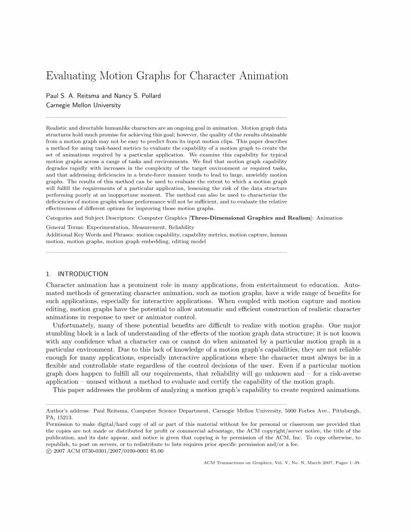
Fig. 1. A motion graph is formed by adding additional transitions between frames of motion capture data. In this diagram,each vertical hashmark is a frame of motion; connecting arrows represent these additional transitions. The frames of Motion1 from ip to iq represent one clip (node) in the motion graph, and the edges of the motion graph are the connections between
clips. The clip represented by the frames from ip to iq , for example, has two incoming edges: one from Motion 2 (blue arrow)and another from frame ip−1 in Motion 1.
3. SYSTEM OVERVIEW
Our system takes as input (1) a set of motion capture data, (2) visual quality requirements for the animations(represented as a model of acceptable motion editing), (3) a set of motion capability requirements (i.e., whattasks the character must be able to accomplish), and (4) an environment in which the character is to performthose tasks. These inputs define the scenario under analysis.
The motion capture data is processed to form a motion graph (see Section 3.1). We further process thismotion graph to capture interactions with the target environment (Section 3.2 and Section 4), based ona model of motion editing (Section 3.3). The resulting data structure is used to measure the animatedcharacter’s ability to successfully complete the required tasks in the given environment (Section 3.4 andSection 5).
3.1 Introduction to Motion Graphs
The following is a brief introduction to the idea of a motion graph; much more detail can be found in thereferences, for example [Kovar et al. 2002].
Normally, motion capture data is played sequentially; to replay the motion of clip i, the animation tran-sitions from frame ik to frame ik+1. The intention of a motion graph is to allow additional flexibility whenusing the motion capture data. The data is examined to find additional transitions of the form ik to jm (i.e.,clip i, frame k to clip j, frame m) that will result in acceptable motions. One common criterion for selectionof such transitions is that frames ik and jm−1 are sufficiently similar.
A motion graph is formed by considering these additional transitions to be the edges of a directed graph(see Figure 1). Nodes in the graph are sequences of frames extending between transitions (e.g., frame ip toframe iq−1), and are referred to in this paper as motion clips. Traversing this graph consists of playing asequence of these clips, with all clip-to-clip boundaries being at one of these additional transitions. To allowcontinuous motion generation, only the largest strongly connected component (SCC) of the motion graph isused.
3.2 Capturing Motion Graph/Environment Interaction
The details of a particular environment can have a very significant impact on the capabilities imparted toan animated character by a motion graph. The simplest example of this is to consider two environments
ACM Transactions on Graphics, Vol. V, No. N, March 2007.

Evaluating Motion Graphs for Character Animation · 5
(a) Empty environ-ment
(b) Environ withtrench
(c) More complex en-viron
(d) Complex environ (3D)
Fig. 2. Example environments. The upper obstacle (blue) in environments (b) and (c) is annotated as a chasm or similarobstacle, meaning it can be jumped over. The environment shown in (c) and (d) is our baseline reference environment.
(Figure 2(a) and 2(b)), one of which has a deep trench bisecting it that must be jumped over; for a motiongraph with no jumping motions, the two environments will induce a very different ratio between the totalspace of the environment and the space which can be reached by a character starting in the lower portion. Amore complex example is shown in Figure 2(c) and 2(d), where small changes to the sizes and positions ofobstacles—changes that may appear superficial—produce very large differences in the ability of the characterto navigate through the environment. Due to this strong environmental influence on the capabilities of amotion graph, the only way to understand how a motion-graph-driven animated character will actuallyperform in a given environment is to analyze the motion graph in the context of that environment.
For any given scenario to be evaluated, we need a way to capture the influence of the environmenton the capabilities of the motion graph. There are a number of possible approaches to capturing theinteraction between an environment and the motion graph; our approach is to embed the motion graph into
ACM Transactions on Graphics, Vol. V, No. N, March 2007.

6 · Paul S. A. Reitsma and Nancy S. Pollard
Fig. 3. A motion clip can be edited to place its endpoint anywhere within its footprint (yellow region). Dotted arrows showthe edited paths corresponding to the possible endpoints (pi, θi) and (pk, θk).
the environment—unrolling it into the environment in the manner described in Section 4.
3.3 Visual Quality Requirements
Embedding a motion graph into an environment so that its capabilities can be measured requires makinga choice of editing model. Generally, the visual quality of motions created in a motion graph will start ata high base due to the verisimilitude of the underlying motion capture data, and will be degraded by anyediting done to the motion, either due to the loss of subtle details or to the introduction of artifacts such asfoot sliding. Such editing is necessary to transition between the different motion clips of the motion graphand to precisely target the character to achieve certain goals (such as picking up an object or walking througha narrow doorway). Additionally, allowing motions to be edited increases the range of motions available tothe animation system, increasing the capabilities of the available animations while decreasing their visualquality.
We assume that current and future research on motion editing and on perceptual magnitude of editingerrors will allow animators to determine the extent to which a motion clip can be edited while maintainingsufficient visual quality to meet the given requirements. Given those bounds on acceptable editing, a motionclip starting at a point p and character facing θ which would normally terminate at a point p′ and facingθ′ can be edited to terminate at a family of points and facings {pi, θi} containing {p′, θ′}. In general, thebetter the editing techniques and the lower the visual quality requirements, the larger this family of validendpoints for a given clip. This family of points is known as the footprint of the motion clip; given a specificstarting point and direction, the footprint of a clip is all of the endpoints and ending directions which it canbe edited to achieve without breaching the visual quality requirements (see Figure 3).
Design of motion editing models is an open problem; we use a simple linear model, meaning the amountof acceptable editing grows linearly with both distance traveled and motion clip duration (see Appendix A),similar to the approach of Sung et al. [2005] and Lee et al. [2006].
3.4 Motion Capability Requirements
We define the capability of a motion graph within an environment as its ability to create motions that fulfillour requirements within that environment. The appropriate metric for evaluating character capabilitiesdepends on the tasks the character is expected to perform. For localized tasks such as punching a target orkicking an object, the task may be to efficiently navigate to the target and contact it with an appropriatevelocity profile, while for some dance forms the task may be to string together appropriate dance sequenceswhile navigating according to the rules of the dance being performed. This paper focuses on navigation
ACM Transactions on Graphics, Vol. V, No. N, March 2007.

Evaluating Motion Graphs for Character Animation · 7
C
B
A
SCC, local reference frame
A
B C
random walk in task domainoriginal motion graph
Fig. 4. (Left) A motion graph may be constructed using a reference frame local to the character to preserve flexibility in thecharacter’s motion. (Right) Using this motion graph to drive the character through an environment with obstacles can resultin dead ends. Because obstacle information is not available in the local reference frame (left), extracting a strongly connectedcomponent (SCC) from the original motion graph does not guarantee that the character can move through a given environmentindefinitely.
and localized actions (such as punching, ducking, or picking up an object). We focus on the followingrequirements, chosen so as to approximate the tasks one might expect an animated character to be requiredto perform in a dynamic scenario, such as a dangerous-environment training simulator or an adventure game:
—Character must be able to move between all major regions of the environment.
—Character must be able to perform its task suite in any appropriate region of the environment; for example,picking up an object from the ground regardless of that object’s location within the environment.
—Character must take a reasonably efficient path from its current position to any specified valid targetposition.
—The previous two items should not conflict; i.e., a character tasked with performing a specific action at aspecific location should still do so efficiently.
—Character must respond quickly, effectively, and visibly to user commands.
4. EMBEDDING INTO THE ENVIRONMENT
In this section, we describe the details of our embedding algorithm. To illustrate the design considerationsfor an embedding approach, consider attempting to compute the value of a sample metric: Simple Coverage.The value of this metric is just the fraction of the environment through which the character can navigatefreely. One immediate challenge is to form a compact description of the space of character trajectories –simply expanding the motion graph in a breadth-first fashion from an arbitrary starting state, for example,will rapidly lead to an exponential explosion in the number of paths being considered. A second key challengeis to consider only paths which do not unnecessarily constrain the ability of the character to navigate. Forexample, avoiding dead ends is necessary for an autonomous character with changing goals, or for a charactersubject to interactive control. Even though the original motion graph has no dead ends, obstacles can causedead ends in the environment (see Figure 4)
In order to meet these challenges, we discretize the environment, approximating it with a regular grid ofcells. At each cell, we embed all valid movement options available to the character. This embedding forms adirected graph, of which we only use the largest strongly connected component (SCC). Note that this SCCis in the embedded graph, not within the original motion graph. For example, in Figure 4, link A is not validat that position within the environment, and so would be discarded for that position only; link A may notbe blocked in other parts of the environment, and hence may be a part of the (embedded) SCC in somepositions and not in others.
ACM Transactions on Graphics, Vol. V, No. N, March 2007.

8 · Paul S. A. Reitsma and Nancy S. Pollard
While computing the embedded SCC has a high one-time cost, that cost is amortized over the manytests run to compute the metrics of interest, each of which is made more efficient by having the informationembodied in the SCC available. This savings can reach many orders of magnitude for metrics such as testingfor availability of efficient paths through the environment. Consider, for example, the problem of searchingfor an optimal path in an environment filled with obstacles. With the embedded graph, paths that leadinexorably to collisions (of which there are many) are not part of the SCC and never need to be considered.Computing this SCC in advance, then, allows efficient computations of the capabilities of the motion graphunder investigation.
4.1 Discretization
We discretize the environment along the following dimensions, representing the state of the character:
X The x-axis groundplane position of the character’s root.
Z The z-axis groundplane position of the character’s root.
Θ The facing direction of the character.
C The clip which brought the character to this (X,Z,Θ) point (i.e., the character’s pose).
C is inherently discrete, but the groundplane position indices (X,Z) are determined by discretizing theenvironment into a grid with fixed spacing distance between adjacent X or Z bins. Similarly, the facing ofthe character is discretized into a fixed number of angular bins.
Typically, a ground-plane position specified by only X and Z is referred to as grid location; adding thefacing angle Θ denotes a grid point; finally, specifying the pose of the character by including the motion clipthat brought the character to that point specifies a grid node in the 4D state space.
Each grid node can be considered a node of a directed graph, where [x, z, θ, c] has an edge to [x′, z′, θ′, c′]if and only if:
—Clip c can transition to clip c′ in the original motion graph
—Given a character with root position (x, z) and facing θ, animating the character with clip c′ places(x′, z′, θ′) within the footprint of c′.
—The character follows a valid path through the environment (i.e., avoids obstacles and respects annotations)when being animated from (x, z, θ) to (x′, z′, θ′) by the edited clip c′.
A pair of nodes (u, v) is known as an edge candidate if the first two criteria hold (i.e., the edge will existunless the environment renders it invalid). Note that collision detection is a part of the third criterion (thatthe character follows a valid path through the environment), and hence is performed every time an edgecandidate is examined.
For example, suppose clip A can be followed by either clip B or clip C in the original motion graph. In theenvironment represented in Figure 5, the starting point ([1, 1, π
2, A] is marked with a blue star, endpoints of
valid edges with green circles, and edge candidates which are not valid edges are marked with red squares.The edge ([1, 1, π
2, A], [5, 1, π
2, C]) is in the embedded graph, since its endpoint is within C’s footprint and
the path to it is valid. By contrast, there is no edge from ([1, 1, π2, A], [5, 0, π
2, C]), since the edited path of
clip C (dotted arrow) is not valid in the environment (it intersects an obstacle).Note that this discretization approach offers a tradeoff between precision and computation. Our metrics
generally give broadly similar results across a range of grid sizes (see Section 6.5), suggesting that the valuescomputed in a discretized setting are reasonable approximations of those values in the continuous case.
4.2 Space-Efficient Unrolling
Reitsma and Pollard [2004] present an embedding algorithm that works by computing all edges and thenusing Depth-First Search to find the largest strongly connected component (SCC). The main limitation of this
ACM Transactions on Graphics, Vol. V, No. N, March 2007.

Evaluating Motion Graphs for Character Animation · 9
Fig. 5. Computing edges from a single node; the endpoints of valid edges are marked as green circles. Note that not all nodeswithin a clip’s footprint are the endpoints of edges, as obstacles can obstruct the edited path from the source to the target node(dotted path).
(a) Seed node (b) Reachable pass 1 (c) Reachable pass 2 (d) Reachable nodes
(e) Reaching pass 1 (f) Reaching pass 2 (g) Reaching nodes (h) SCC
Fig. 6. Steps of the embedding algorithm. (a) A seed node (green ”S”) is chosen. (b) First pass of the reachable flood marksnodes reachable in one step from the seed node. (c) Second pass marks additional nodes reachable in two steps. (d) All reachablenodes are marked (blue vertical hashes). (e) First pass of the reaches flood marks nodes which reach the seed node in one step.(f) Second pass marks additional nodes reaching in two steps. (g) All reaching nodes are marked (red horizontal hashes). (h)
Intersection of set of reachable nodes and set of reaching nodes (purple ”+”) is the SCC of the embedded graph.
algorithm is that it requires explicitly storing all edges needed to compute the embedded graph. While thisis an efficient and sensible approach for smaller environments or coarser grids, due to memory considerationsit significantly limits the size of environments and the resolution at which they can be processed.
As an alternative that requires much less memory, we propose a flood-based algorithm which takes ad-vantage of the fact that edges outgoing from or incoming to a node can be computed only as needed. Forgrid nodes u and v, an edge candidate (u, v) will be in the SCC if and only if nodes u and v are both in theSCC, and (u, v) is an edge of the embedded graph (i.e., its associated path is valid within the environment),so storing only the nodes in the SCC allows computation of the correct edges as needed.
Finding the SCC for use with this on-the-fly approach can be done efficiently in the discretized environment
ACM Transactions on Graphics, Vol. V, No. N, March 2007.

10 · Paul S. A. Reitsma and Nancy S. Pollard
(see Figure 6):
—Choose a source node s (green ”S”).
—Flood out from s, tagging all reachable nodes (blue vertical hashes).
—Flood into s, tagging all nodes reaching it (red horizontal hashes).
—Intersection of the two tagged sets is the SCC (purple ”+”).
In practice, motion graphs embedded into environments typically result in an embedded graph with asingle SCC whose number of nodes is linear in the total number of nodes in the environment which are notobstructed by obstacles1; 10-25% of the total number of nodes in the environment is a typical size for anSCC. Accordingly, s can be chosen uniformly at random until a node inside the SCC is found without anasymptotic increase in time2.
Flooding is done using a multi-pass Breadth-First Search. For finding the set of Reachable nodes, bit arraysare used to tag which nodes are Active or Reached. Initially only s has its Active bit set, and no nodeshave their Reached bits set. At each pass, the algorithm iterates through each node k in the environment.If Active(k) is set, then k is expanded. Expanding a node consists of setting Reached(k) to true, settingActive(k) to false, and finding the set of edges for k3. For each of those edges j, Active(j) is set if and onlyif Active(j) and Reached(j) are both false (i.e., j has not been tagged or expanded yet). The algorithm endswhen there is no node k such that Active(k) is set.
Since any node’s Active bit is set to true at most once, the algorithm terminates. Since all nodes reachablefrom s will have their Active bit set, the algorithm correctly computes the set of nodes reachable from s.Each pass of the algorithm may touch every node in the environment, but each edge is expanded only onceper flood direction. Accordingly, the runtime of the algorithm is the cost of computing whether each edgeis valid in the environment plus the cost of reading each node’s tags for each iteration until until the searchis complete; i.e., Θ(e) + Θ(D ∗ N), for e the number of edges in the SCC, N the number of nodes in theenvironment, and D the diameter of the embedded graph (i.e., the maximum depth of the Breadth-FirstSearch). In practice, the Θ(e) term dominates, making the algorithm approximately as efficient as regularBreadth-First Search.
The set of nodes which can reach s is computed analogously; however, since the set of reachable nodesin already known, only those nodes need to be expanded, as no other nodes can be in the SCC. This offerssubstantial computational savings.
Note that storing the Reachable and Reaching sets requires two bits of storage per node, and that anotherbit is required as scratch memory for the Active set, for a total memory requirement of three bits per node.
4.2.1 Space Complexity. We can estimate the theoretical space complexity of the embedded graph withrespect to the parameters affecting it. For a given environment, the number of nodes in the embedded graphis
O(n) = O(AxzaC) (1)
1There is some evidence this should be expected; see, for example, [Muthukrishnan and Pandurangan 2005] regarding thisproperty in random geometric graphs.2In practice, the actual overhead is minimal if fast-fail tests are used. Testing that source nodes have at least 5,000 reaching
and reachable nodes efficiently rejects most nodes outside the SCC; in our experiments, testing that the source node can reachitself was the only other fast-fail test required.3Recall from Section 4.1, an edge from node [x, z, θ, c] to node [x′, z′, θ′, c′] exists if and only if (1) clip c can transition toclip c′ in the original motion graph, (2) starting the character at position (x, z, θ) and animating it with clip c′ will place
(x′, z′, θ′) within that clip’s footprint, and (3) the resulting path is valid in the environment (i.e., avoids obstacles and respectsannotations).
ACM Transactions on Graphics, Vol. V, No. N, March 2007.
Evaluating Motion Graphs for Character Animation · 11
and the number of edges in the embedded graph is
O(e) = O(Ax2z2a2Cb) = O(nxzab) (2)
where:
A = the accessible (i.e., character would not collide with an obstacle) area of the environment, in m2.
x = the discretization of the X axis, in grid cells per m.
z = the discretization of the Z axis, in grid cells per m.
a = the discretization of the character’s facing angle, in grid cells per 2π radians.
C = the number of motion clips used (i.e., the number of nodes in the original motion graph).
b = the mean branching factor of the original motion graph.
Equation 1 simply notes that the number of nodes in the SCC is linear in the total number of nodesinto which the environment is discretized. Equation 2 demonstrates how the average number of edges pernode is constant with increasing environment size, but increases linearly with increasing resolution (in eachdimension), due to more grid points being packed under each clip’s editing footprint. Note that a clip’sediting footprint increases in size with the length and duration of the clip, but that enforcing a minimumand maximum clip duration when creating the motion graph ensures two clips’ footprints will differ in areaby at most a constant factor.
The one-step unrolling algorithm presented in [Reitsma and Pollard 2004] stores the edges of this embeddedgraph explicitly, and so has space complexity O(nxzab). By contrast, the flood-based algorithm presentedhere has space complexity O(n); i.e., linear in the number of nodes in the embedded graph, rather thanin the number of edges, meaning the amount of memory required is reduced by a factor of Θ(xzab). Inpractice, the big-Theta notation hides an additional large constant factor of improvement, as only a few bitsare required to compute and store each node.
The empirical scaling behavior of these two algorithms with respect to environments of increasing size isexamined in Section 6.4.3.
4.2.2 Time Complexity. While the space-efficient algorithm requires asymptotically less space than theone-step unrolling algorithm, it typically does not require asymptotically more time.
The algorithm of Reitsma and Pollard [2004] computes each edge candidate in the environment once,stores valid edges, and accesses each cached edge twice when using Depth-First Search to find the SCC. Theruntime for this algorithm is:
Trp04 = Θ(oNbf + 2E) = Θ(oE + 2E) = Θ(oE) (3)
where N is the number of unobstructed nodes in the environment, f is the mean number of nodes underthe footprint of a clip, E is the number of edges in the environment, and o is the mean number of obstacle-intersection tests required when computing each edge.
When expanding a node, the algorithm of Section 4.2 computes either incoming edge candidates or outgoingedge candidates. As a node will be expanded only once in each direction (Reachable/Reaching), each outgoingedge candidate from that node and each incoming edge candidate to that node will be computed only oncewhen finding the SCC. Accordingly, the runtime of our algorithm is:
Tflood = Θ(onrbf + onbf ′) = O(oE) (4)
where nr is the number of nodes reachable from the SCC, and f ′ is the mean number of nodes under thereverse footprint of a clip (i.e., the set of start points {p, θ} such that the footprint of clip c played from thatpoint will contain the end point (p′, θ′)).
ACM Transactions on Graphics, Vol. V, No. N, March 2007.
12 · Paul S. A. Reitsma and Nancy S. Pollard
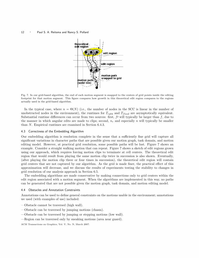
Fig. 7. In our grid-based algorithm, the end of each motion segment is snapped to the centers of grid points inside the editingfootprint for that motion segment. This figure compares how growth in this theoretical edit region compares to the regionsactually used in the grid-based algorithm.
In the typical case, where n = Θ(N) (i.e., the number of nodes in the SCC is linear in the number ofunobstructed nodes in the environment), the runtimes for Trp04 and Tflood are asymptotically equivalent.Substantial runtime differences can occur from two sources: first, f ′ will typically be larger than f , due tothe manner in which angular edits are made to clips; second, nr and especially n will typically be smallerthan N . Empirical runtimes are examined in Section 6.4.3.
4.3 Correctness of the Embedding Algorithm
Our embedding algorithm is resolution complete in the sense that a sufficiently fine grid will capture allsignificant variations in character paths that are possible given our motion graph, task domain, and motionediting model. However, at practical grid resolution, some possible paths will be lost. Figure 7 shows anexample. Consider a straight walking motion that can repeat. Figure 7 shows a sketch of edit regions grownusing our approach, which requires forcing motion clips to terminate at cell centers. The theoretical editregion that would result from playing the same motion clip twice in succession is also shown. Eventually,(after playing the motion clip three or four times in succession), the theoretical edit region will containgrid centers that are not captured by our algorithm. As the grid is made finer, the practical effect of thisapproximation will decrease, and we discuss the results of experiments testing the stability to changes ingrid resolution of our analysis approach in Section 6.5.
The embedding algorithms are made conservative by making connections only to grid centers within theedit region associated with a motion segment. When the algorithms are implemented in this way, no pathscan be generated that are not possible given the motion graph, task domain, and motion editing model.
4.4 Obstacles and Annotation Constraints
Annotations can be used to define general constraints on the motions usable in the environment; annotationswe used (with examples of use) included:
—Obstacle cannot be traversed (high wall).
—Obstacle can be traversed by jumping motions (chasm).
—Obstacle can be traversed by jumping or stepping motions (low wall).
—Region can be traversed only by sneaking motions (area near guard).
ACM Transactions on Graphics, Vol. V, No. N, March 2007.
Evaluating Motion Graphs for Character Animation · 13
—Region cannot be traversed by jumping motions (normal locomotion should not be assumed to includejumping for no reason).
—Picking-up motions should not be used unless the user selects the action.
Most of these annotations—either defining different obstacle types which interact differently with differentmotion types, or defining regions where the character must act in a certain way—are self-explanatory, andare handled automatically during collision-detection; any path which violates an annotation constraint willnot be expanded, and hence cannot contribute to the embedded graph. Annotations such as the last one aremore complicated, as some motions need to be designated as strictly-optional (and hence cannot be used toconnect parts of the embedded graph) but readily-available. We refer to these as selective actions.
4.5 Selective Actions
Selective actions are those actions which must be strictly optional (i.e., selectable by the user at will, butotherwise never occurring in unconstrained navigation). A user may choose to have the character perform apicking-up action when there are no nearby objects on the floor, for example, but it would look very strangefor such a spurious pick-up action to show up in automatically-generated navigation.
An embedded graph created from all motions will not respect this requirement; in particular, parts ofthe environment may be reachable only via paths which require selective actions, rather than by regularlocomotion, and hence those parts of the environment should not be considered reachable.
Selective actions are handled by a slight modification to the embedding algorithm. First, the embeddingalgorithm described previously is run with only those actions deemed “locomotion” permitted; all otheractions are deemed “selective”, and are not expanded, although any selective-action nodes reached aremarked as such. An exception is made for selective actions which are necessary for traversing an annotatedobstacle; e.g., jumping motions are permitted only insofar as they are required to traverse obstacles suchas the jumpable-chasm obstacle in Figure 2(b). This creates a backbone embedded graph composed oflocomotions.
Next, for each reachable selective action, nodes from all valid paths of reasonable length are added to theembedded graph. The result may not be a strongly connected component, since some of the added pathsmay not rejoin the SCC; accordingly, the embedding algorithm is rerun (as illustrated in Figure 6) to findthe new strongly connected component. This time, however, the resulting SCC must be a subset of theprevious embedded graph (i.e., the original SCC plus the added paths); hence, that information can be usedto substantially reduce the number of nodes expanded by the embedding algorithm. The resulting embeddedgraph, known as the augmented SCC will automatically include all reachable selective actions which can inturn reach the backbone SCC by paths of reasonable length, and will include all such rejoining paths.
The cost for creating this augmented SCC is the cost for creating the initial SCC, plus the cost of addingin paths from each selective action out to a fixed depth, plus the cost of re-running the flooding algorithmon this subset of nodes. The total cost is:
Taug = Tflood + Tpaths + Tflood′ = O(oE) + O(onbfh) + O(oE) = O(oE) (5)
where h is the mean depth in edges of the added paths. Comparing to Equation 4, computing the augmentedembedded graph is asymptotically equivalent to computing the regular motion graph with all motions treatedequally, and in practice requires about twice as much computation time. In addition, storing the “selective”actions during computation of the initial embedded graph and storing that initial SCC during computationof the final, augmented SCC requires an extra bit of storage per node, for a total cost of four bits per nodein the environment.
We used this type of embedded graph for all of our experiments.
ACM Transactions on Graphics, Vol. V, No. N, March 2007.
14 · Paul S. A. Reitsma and Nancy S. Pollard
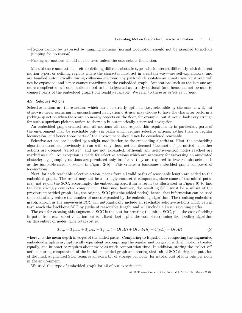
Fig. 8. A grid cell is covered by a clip if that clip’s footprint includes the cell’s center. (Covered grid cells are in green.)
5. MOTION GRAPH CAPABILITY METRICS
To measure the capability of a motion graph, we define metrics which evaluate the motion graph’s ability tofulfill the requirements identified in Section 3.4.
5.1 Environment Coverage
The most basic problem a motion graph can have in an environment is simply that it is unable to navigatethe character effectively enough to access large regions of that environment. Accordingly, the environmentcoverage metric is designed to capture the ability of the character to reach every portion of its workspacewithout becoming irretrievably stuck, similar to the viability domain from viability theory (see, for example,Aubin [1990]). For navigation, this workspace is represented by discretized grid points {X,Z,Θ} (see Section4.1).
We define grid point (X,Z,Θ) as covered by clip c if the center of (X,Z,Θ) is within the footprint of c
(see Figure 8).4 From this occupancy information we compute Environment Coverage as:
CXZA =
∑
i covered(i)∑
i collisionFree(i)(6)
where the numerator contains a count of all 3D grid points which are covered by at least one clip in theembedded graph, and the denominator contains a count of all grid positions which are theoretically validfor character navigation (i.e., some motion type exists for which the character would not collide with anobstacle or violate an annotation constraint; see Figure 9). CXZA is a discretized estimate of the fraction ofviable (x, z, θ) workspace through which the character can navigate under arbitrary control. CXZ , the 2Dequivalent, can be defined analogously.
Regions with low or no coverage typically indicate that the entrances to those regions from the rest ofthe environment are highly constricted, and there are few ways to place the motions required to enter thatregion without colliding with obstacles or violating annotation constraints.
5.2 Action Coverage
The coverage for action k is defined analogously to Environment Coverage. The 2D version is:
CXZ,k =
∑
i coveredk(i)∑
i collisionFree(i)(7)
4An alternative definition of coverage is that any grid point containing any root position of any frame of any clip is covered. Inpractice, these definitions give essentially identical results, but the former definition is significantly faster to compute.
ACM Transactions on Graphics, Vol. V, No. N, March 2007.

Evaluating Motion Graphs for Character Animation · 15
Fig. 9. Coverage over a simple environment. Obstacles are in red; covered areas are in grey. Brighter grey means more coverage(i.e., the grid location is covered by more clips).
where coveredk(i) is true if and only if there exists an edge in the embedded graph such that animating thecharacter with that edge causes the central frame of action k to occur in grid location i.
5.3 Path Efficiency
The path efficiency metric is designed to evaluate the ability of the motion graph to allow the characterto navigate efficiently within the accessible portion of the environment. Each path will have a particularvalue for path efficiency, and hence the goal is to estimate the distribution of path efficiencies over the setof all possible paths through the environment. To estimate this distribution, we must make an assumptionabout the manner in which paths will be specified. For this paper, we examine the problem of point-to-pointnavigation, where the (X,Z) values of start and end points are specified (such as with a mouse) and a pathmust be found for the character to travel between these two points5. Ideally, a near-minimal-length pathwould exist for all pairs of start and end positions. The metric for relative path length in point-to-pointnavigation is:
EP =pathLength
minPathLength(8)
where pathLength is the length of the shortest path available to the character from the start point to theend point and minPathLength is the length of an ideal reference path between those two points (see Figure10).
When evaluating the path efficiency ratio of a (start, end) pair, we work with the embedded graph describedin Section 4. Using this graph ensures that only paths which do not result in dead ends are considered, andalso significantly improves the efficiency of shortest path calculations.
Given this embedded graph, we use Monte Carlo sampling to estimate the distribution of path efficiencyratios within the 4D space defined by all valid (start, end) pairs. Start and end positions are selecteduniformly at random from the set of grid positions which have non-zero coverage (see Section 5.1). ValuepathLength, the shortest path available to the character, is computed using A* search through the embeddedgraph. Value minPathLength, the shortest path irrespective of available motions, is estimated using A*search over the discretization grid imposed on the environment, with each 2D (X,Z) grid location beingconnected to all neighbors within five hops in either X or Z (i.e., an 11x11 box). Path efficiency is thencomputed as in Equation 8.
Due to the highly discrete nature of motion graphs, extremely short paths may have unrepresentative pathefficiency ratios according to the presence or absence of a clip of particular length in the motion graph; to
5Several similar definitions of this metric are possible, such as accepting paths that pass through the target point, rather than
only ones ending there. In practical embedded graphs, the results will tend to be very similar, but the definition used here canbe computed more quickly, and is closer to the “go to the click” interaction paradigm which motivates the metric.
ACM Transactions on Graphics, Vol. V, No. N, March 2007.

16 · Paul S. A. Reitsma and Nancy S. Pollard
Fig. 10. Paths through a simple environment. Obstacles are in bright red, the minPathLength path is in deep red, and thepathLength path is in green (starting point is marked with a wider green dot). (Left) A typical path. (Right) The theoreticalminPathLength path can head directly into the wall, while the pathLength path, which relies on motions in the SCC, must end
in a state that allows for further movement.
reduce this erratic influence and to consider paths more representative of typical user-controlled navigationaltasks, we throw away (start, end) pairs whose linear distance is less than 4m and re-select start and endcandidates. Since the space complexity of A∗ grows exponentially with path depth and we expect moresophisticated planning algorithms will be used in practice, we similarly throw out (start, end) pairs whoseminPathLength is greater than 7m. We believe such longer paths will not have significantly different pathefficiency distributions from paths in the 4 − 7m range, due to the ability to chain shorter paths togetherto create long ones. Note also that extremely slow-moving motions, such as idling in place, can skew theresults. We treat each clip as having a minimum effective speed of 0.5m/s for the purposes of minimumpath computation in order to help filter out spurious paths such as ones which make all turns by stoppingand turning in place. Note that this speed is virtual only; while a path which includes two seconds of idlingwould have an additional 1m added to its length during the search for the shortest path, if selected its truelength would be used to calculate the path efficiency ratio.
A poor score on the Path Efficiency metric usually results from the most direct route between the startand end locations passing through areas of very limited coverage (and, hence, very limited path options).
5.4 Action Efficiency
This metric measures the efficiency overhead required to execute a desired action, such as picking up an objectlying on the floor across the room. The metric is measured in a Monte Carlo fashion exactly analogous tothat described for Path Efficiency:
AEa =pathLengtha
minPathLength(9)
where a is the action type in question, minPathLength is the length of the reference path computed exactlyas per the path efficiency metric, and pathLengthA is the length of the shortest path through the embeddedgraph that ends in a clip which executes an instance of action a in the end location.
High values of this metric as compared to the Path Efficiency value for the same (start, end) pair typicallyrepresent actions which are inflexibly linked into the motion graph, such as a ducking motion which can onlybe accessed after running straight for several meters, and which are coupled with or consist of motions whichdo not fit well into regions of the environment (such as a region requiring twisty paths between obstacles).
5.4.1 A* Planner. Our A* planner uses the following as a conservative distance estimate:
Dest = DS→X + ||X − E|| (10)
ACM Transactions on Graphics, Vol. V, No. N, March 2007.

Evaluating Motion Graphs for Character Animation · 17
where Dest is the heuristic estimate of distance from the start point S to the end point E, DS→X is thelength of the path currently being examined, and ||X −E|| is the linear distance between X, the end of thecurrent path, and E.
Note that our A* path planner returns the optimal path between the specified start and end locations;applications which use a different style of planner which sometimes returns sub-optimal paths will havecommensurately-worse path-based metric results. In the more demanding environments, some of the optimalpaths initially move a substantial distance away from the end location, so a path planner with a limitedhorizon would generate paths that were longer or even substantially longer than optimal, which would resultin a worse score on both the Path Efficiency and the Action Efficiency metrics.
5.5 Local Maneuverability
Inspired by the idea of local controllability [Luenberger 1979], the local maneuverability metric is designed toevaluate the responsiveness of the character to interactive user control. In many interactive applications, ahighly responsive character is critical; in a hazardous-environment training scenario, for example, a significantlag in character response would not only be immensely frustrating and interfere with training, but couldactually teach bad habits; for example, if a character is unable to transition rapidly into evasive behaviors,users may simply learn to avoid using such behaviors, even in situations where they would be appropriate.
The instantaneous local maneuverability of a character is simply the mean amount of time required for thatcharacter to perform any other action which is currently valid. At a particular moment, the instantaneouslocal maneuverability of the character with regard to action k is:
LMk(t) = (1 − α(t)) ∗ Dc0+ MDPk (11)
where c0 is the currently-playing clip, α(t) is the fraction of that clip already played at time t, Dc is theduration in seconds of clip c, and MDPk is the shortest possible time to reach an instance of motion type k
from the end of the current path while following paths from the motion graph. For example, if the characteris 0.3s from the end of a running clip and the minimum-time path from the end of that clip to an instanceof punching is 1s, then the character’s Local Maneuverability with respect to punching is 1.3s.
The character’s overall Local Maneuverability is the weighted sum of its per-action Local Maneuverabilities:
LM(t) =1
||K||
∑
k∈K,k 6=Tc0
(wk ∗ LMk) (12)
where K is the set of actions which are in the motion graph and currently valid, and wk is the weight foraction type k. This gives an overall measure of the character’s ability to respond to external control, takinginto account the different reactivity needs of the different motion types (i.e., evasive actions such as duckingmay need to be available much more rapidly than actions such as picking up an object).
There are two ways to measure expected overall local maneuverability. The first is Theoretical LocalManeuverability, which is measured in the original motion graph:
LMT,k =1
||C||
∑
c∈C
(0.5 ∗ Dc + MDMPc,k) (13)
where C is the set of all clips in the motion graph and MDMPc,k is the duration in seconds of the minimumduration path through the motion graph from the end of clip c to any instance of motion type k. This givesa baseline for what instantaneous local maneuverability a character can be expected to have at any timeunder ideal conditions (i.e., the environment does not invalidate any of the minimum-duration paths). Poortheoretical local maneuverability values typically indicate poor connectivity between motion types in themotion graph.
ACM Transactions on Graphics, Vol. V, No. N, March 2007.

18 · Paul S. A. Reitsma and Nancy S. Pollard
By contrast, in-practice or Practical Local Maneuverability computes the expected instantaneous localmaneuverability from each node of the embedded graph:
LMP,k =1
||G||
∑
n∈G
(0.5 ∗ Dcn+ MDEPcn,k) (14)
where G is the set of nodes in the embedded graph, cn is the clip associated with embedded graph node n,and MDEPc,k is the duration in seconds of the minimum duration path through the embedded graph fromthe end of clip c to an instance of motion type k. This gives an expectation for what instantaneous localmaneuverability a character can be expected to have at any time when navigating through the environmentin question. Comparing this to its theoretical equivalent can provide information about the restrictions theenvironment places on responsiveness to user control.
Note that computing local maneuverability for every node is computationally expensive; in practice, weuse a subset of nodes selected uniformly at random (i.e., 1% sampling means any particular node was used inthe calculation with probability 0.01). The stability of the result at different sampling densities is examinedin Section 6.5.
Finally, note that local maneuverability can be computed for many slices of the data; of note are:
—Computing the local maneuverability for a single action which needs to be rapidly accessible at all times(such as evasive ducking).
—Computing the local maneuverability from one subset to another, such as from locomotions to all evasivemaneuvers.
—Computing the local maneuverability from locomotions to same-type locomotions with the character’sfacing turned more than N degrees clockwise from the starting facing, in order to gain a local measure ofthe character’s ability to respond rapidly to a user’s navigational directions (such as “run into that alcoveto the left to avoid the boulder rolling at you”).
—Computing statistical information on any of the above by examining the distribution of local maneuver-ability values over all nodes. Information about extremal values, such as how often it would take greaterthan 3 seconds to reach an evasive motion, can be particularly informative.
6. RESULTS
6.1 Example Scenarios
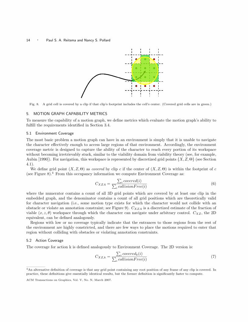
The two components of a test scenario are the motion graph used and the environment in which it is em-bedded. Our primary test environment was a large room with varying levels of clutter (Figure 11(c)). Thisroom measures 15m by 8m, and our primary testing resolution used a grid spacing of 20cm by 20cm forthe character’s position and 20 degrees for the character’s facing angle. We include results from other en-vironments, including tests on randomly-generated environments of varying sizes and configurations, andother discretization grid resolutions. To take into account obstacles, we do collision detection with a cylin-der of radius 0.25m around the character’s root, although more exact collision detection algorithms (e.g.,[Gottschalk et al. 1996]) could be plugged in seamlessly; hence, all obstacles can be described as 2D shapeswith annotations.
All motion graphs used were computed using motions downloaded from the CMU motion capture database(mocap.cs.cmu.edu). Our dataset consisted of 50 motion clips comprising slightly over seven minutes of cap-tured motion, with significant amounts of unstructured locomotion (running, sneaking, and idling), severalexamples each of several actions (jumping, ducking, picking up an object from the floor, punching, andkicking an object on the floor), and transitions between the locomotions and some of the (locomotion,action)
ACM Transactions on Graphics, Vol. V, No. N, March 2007.
Evaluating Motion Graphs for Character Animation · 19
(a) Empty (b) Random (c) Baseline
Fig. 11. Evaluation environments of increasing complexity. The upper obstacle (blue) in environment (c) is annotated as achasm or similar obstacle, meaning it can be jumped over.
pairs (sneak+duck, run+duck, run+punch, run+kick, sneak+pickup, etc.). Each source motion was labeledwith the types of motions it contained, as well as the start, center, and end times of actions.
The per-pair values of adding a transition between any pair of frames were computed using the techniqueof Lee et al. [2002]. The resulting matrix of transition costs was processed in a globally-greedy manner toidentify local maxima (see Appendix B) and to enforce user-specified minimum and maximum clip lengths.Our primary motion graph consisted of 98 nodes (clips) connected by 288 edges, representing 1.5 minutes ofmotion capture data with eight distinct types of motion. We also include results from larger motion graphscontaining additional examples of the same types of behavior.
Our embedding algorithm was implemented in Java and used a simple hash table of fixed size to cachenodes’ edge lists during metric evaluation, with hash table collisions being resolved by a simple hit-vs-missheuristic. Running on a 3.2GHz Xeon computer, finding the final (augmented) embedded graph requiredabout 6.7 minutes and produced an embedded graph with 218K nodes and 1.88M edges.
When playing back motion through the embedded graph, transitioning from the end of motion clip A tothe start of clip B was done by warping the first frame of clip B to match the last frame of clip A, andthen using quaternion splines to smoothly remove that warping over the following 0.5s. Motion editing towarp clips to grid centers was done using displacement splines on the root translation and facing angle. Thisediting technique of course creates footsliding artifacts, which should be cleaned up in post-processing.
6.2 Baseline
Table I shows evaluation results from our basic test scenarios. XZ Coverage is the fraction of collision-free(X,Z) grid cells in the environment which contain at least one node of the embedded graph; XZA Coverageis the analogous quantity taking into account character facing (see Section 5.1). Local Maneuverability(Section 5.5) is the minimum-duration path from a running motion to an instance of the “pick” action ineither the original motion graph (Theoretical LM) or the embedded graph (Practical LM). Path Efficiencyis the ratio of the distances of the shortest point-to-point path in the embedded graph vs. an ideal referencepath (Section 5.3), and Action Efficiency is the ratio of the distances of the shortest path ending in a “pick”motion vs. the same ideal reference path (Section 5.4). All of these paths are optimal for their particularstart and end locations, so the Median Path Efficiency, for example, is the efficiency of the optimal path for
ACM Transactions on Graphics, Vol. V, No. N, March 2007.

20 · Paul S. A. Reitsma and Nancy S. Pollard
Environ Coverage(%) Local Maneuv Path Efficiency Action Efficiency
XZ XZA Theory Prac Mean Median Mean Median
Empty 99.8 94.1 3.6s 4.4s 1.00 1.00 1.25 1.11
Random 94.3 66.5 3.6s 5.6s 1.21 1.03 1.93 1.85Baseline 95.7 60.6 3.6s 6.6s 1.87 1.11 2.85 2.59
Table I. Evaluation results for the three basic test scenarios. Capability steadily worsens as the environments become morecongested with obstacles, as shown by the across-the-board increase of all metric values.
a typical pair of start and end points. Accordingly, any scenario with poor Path Efficiency has a poor valuefor that metric in the optimal case, so a path at “90% Path Efficiency” means the optimal path for thatparticular start and end location was less efficient than the optimal paths for 90% of the other (start, end)pairs chosen.
Results for the environment with no obstacles are excellent, suggesting that the process of discretizationand analysis does not unduly affect the capabilities of the motion graph. Note, however, how Practical LocalManeuverability and Action Efficiency show mobility is slightly affected, largely by the walls surroundingthe environment removing some path options.
The environment with randomly-placed obstacles is relatively open, but represents a much more realisticenvironment, with more interesting evaluation results. XZ Coverage is still high (94.3%), but XZA Coverageis much lower (66.5%), reflecting congested regions which the character can only traverse along a single axis.Median Path Efficiency is still very close to the optimum, but the mean path is over 20% longer than thereference path, meaning that some regions of the environment are difficult for navigation and require verylong paths. This is reflected more strongly in the sharply higher values for Practical Local Maneuverabilityand especially for Action Efficiency. The latter is especially interesting; even the median paths were much(85%) longer than the reference paths, suggesting that the motion graph requires a sizeable open region toefficiently set up and use motions such as “pick”s.
The performance of the default motion graph in the Baseline Environment – the most obstacle-dense ofthe three – is quite poor, especially with respect to having the character use specific actions in specific partsof the environment. The high XZ Coverage value (95.7%) indicates that the character can reach almostany point in the environment; however, the lower XZA Coverage value (60.6%) – reflecting restrictions onthe character’s facing at many points in the environment – indicates the character may have a restrictedability to maneuver at many points. We see that most point-to-point paths through the embedded graph arestill relatively efficient (median was 11% longer than reference), although interactions with highly congestedregions of the environment cause a significant number of exceptions (Figure 12).
By contrast, the mean time from any frame to the nearest “pick” action in the embedded graph is almostdoubled (3.6s to 6.6s) from its already-high value in the original motion graph, and is substantially worsethan the equivalent measurement in the relatively-cluttered Random Environment. Accordingly, we observesubstantial difficulty in creating efficient point-to-point paths which end in a specific action, such as a “pick”motion; even typical paths (Figure 13) are about 160% longer than the ideal reference paths (see Table I,Action Efficiency (Median)).
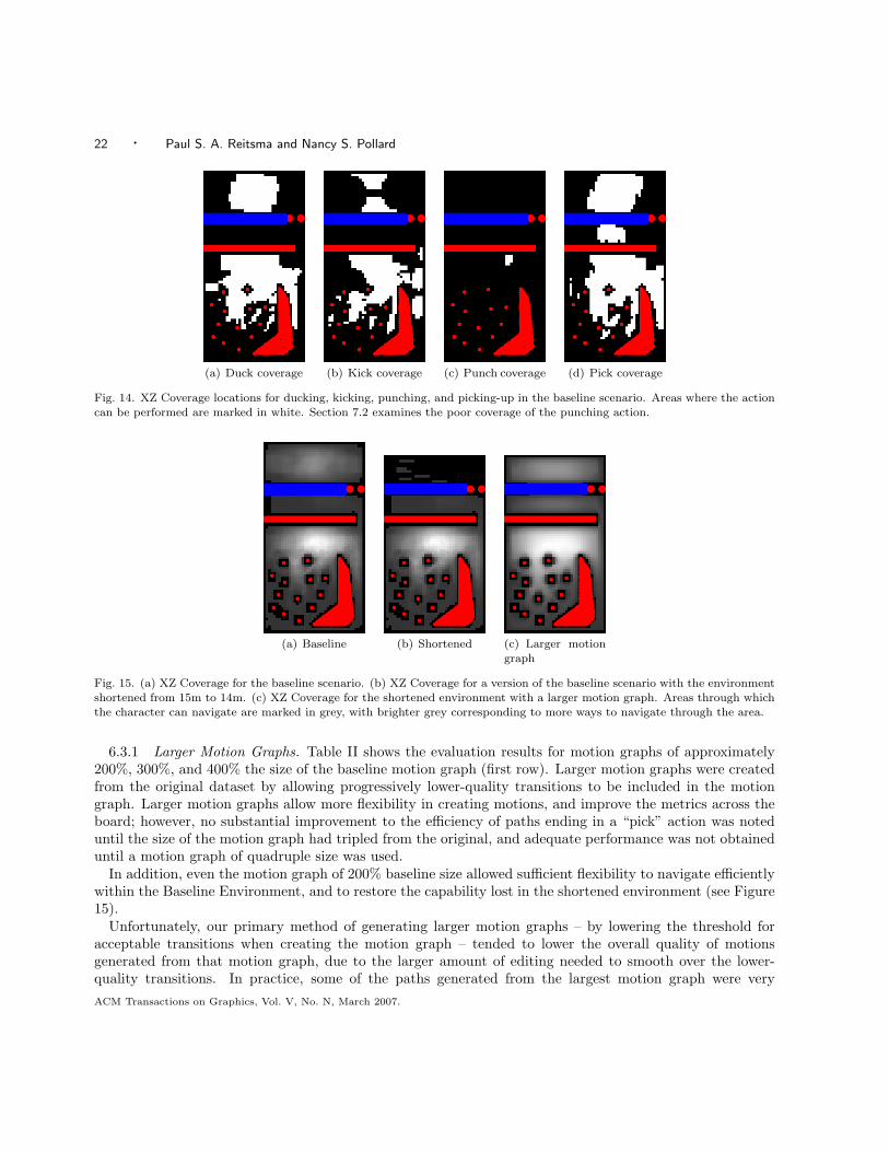
Of the discrete actions available in our motion graph (i.e., pick, duck, kick, punch), the range of areas inwhich each could be used varied widely (see Figure 14). In addition, a slight modification to the BaselineEnvironment radically changed the coverage pattern (see Figure 15).
Section 6.3 examines several potential approaches for improving the performance of motion graphs in thisenvironment. Section 6.4 explores how this evaluation approach scales with increasing size and complexityof scenarios, as well as the effects of our on-demand edge computation algorithm. Finally, specifying a setof metrics required making several assumptions, the validity of which are examined in Section 6.5.
ACM Transactions on Graphics, Vol. V, No. N, March 2007.

Evaluating Motion Graphs for Character Animation · 21
(a) Good path(10th percentile)
(b) Median path(50th percentile)
(c) Bad path(90th percentile)
Fig. 12. Representative character navigation paths in the baseline scenario. The best paths actually available to the characterare in green, ideal reference paths are in dark red. The starting point of the actual path is drawn slightly widened. A 10th
percentile path means that, of all the (start,end) pairs tested, only 10% resulted in a better Path Efficiency metric score (i.e.,
had a ratio between optimal path actually available to the character and ideal reference path that was lower).
(a) Good path(10th percentile)
(b) Median path(50th percentile)
(c) Bad path(90th percentile)
Fig. 13. Representative character pick paths in the baseline scenario. Best-available paths ending in a pick action are in darkgreen and ideal reference paths are in dark red. The starting point of the actual path is drawn slightly widened. A 10th
percentile path means that, of all the (start,end) pairs tested, only 10% resulted in a better Path Efficiency metric score (i.e.,
had a ratio between optimal path actually available to the character and ideal reference path that was lower).
6.3 Improving Motion Graphs
We examine the effects of three common techniques which can be used to improve the flexibility of acharacter’s performance when using a motion graph:
(1) Adding more motion data
(2) Allowing more motion editing
(3) Increasing inter-action connectivity
ACM Transactions on Graphics, Vol. V, No. N, March 2007.
22 · Paul S. A. Reitsma and Nancy S. Pollard
(a) Duck coverage (b) Kick coverage (c) Punch coverage (d) Pick coverage
Fig. 14. XZ Coverage locations for ducking, kicking, punching, and picking-up in the baseline scenario. Areas where the action
can be performed are marked in white. Section 7.2 examines the poor coverage of the punching action.
(a) Baseline (b) Shortened (c) Larger motiongraph
Fig. 15. (a) XZ Coverage for the baseline scenario. (b) XZ Coverage for a version of the baseline scenario with the environmentshortened from 15m to 14m. (c) XZ Coverage for the shortened environment with a larger motion graph. Areas through whichthe character can navigate are marked in grey, with brighter grey corresponding to more ways to navigate through the area.
6.3.1 Larger Motion Graphs. Table II shows the evaluation results for motion graphs of approximately200%, 300%, and 400% the size of the baseline motion graph (first row). Larger motion graphs were createdfrom the original dataset by allowing progressively lower-quality transitions to be included in the motiongraph. Larger motion graphs allow more flexibility in creating motions, and improve the metrics across theboard; however, no substantial improvement to the efficiency of paths ending in a “pick” action was noteduntil the size of the motion graph had tripled from the original, and adequate performance was not obtaineduntil a motion graph of quadruple size was used.
In addition, even the motion graph of 200% baseline size allowed sufficient flexibility to navigate efficientlywithin the Baseline Environment, and to restore the capability lost in the shortened environment (see Figure15).
Unfortunately, our primary method of generating larger motion graphs – by lowering the threshold foracceptable transitions when creating the motion graph – tended to lower the overall quality of motionsgenerated from that motion graph, due to the larger amount of editing needed to smooth over the lower-quality transitions. In practice, some of the paths generated from the largest motion graph were very
ACM Transactions on Graphics, Vol. V, No. N, March 2007.

Evaluating Motion Graphs for Character Animation · 23
Coverage(%) Local Maneuv Path Efficiency Action Efficiency
Clips XZ XZA Theory Prac Mean Median Mean Median
98 95.7 60.6 3.6s 6.6s 1.87 1.11 2.85 2.59
190 98.3 90.3 3.3s 4.6s 1.11 1.01 2.36 2.10282 98.3 91.5 3.6s 3.9s 1.06 1.01 1.47 1.37
389 98.3 95.5 2.6s 3.0s 1.02 1.00 1.20 1.11
Table II. Evaluation results by size of motion graph (see Section 6.3.1). All metric values show substantial improvement,although different tasks improve at different rates.
Edit Coverage(%) Local Maneuv Path Efficiency Action Efficiency
Size XZ XZA Theory Prac Mean Median Mean Median
75% 40.5 17.2 3.6s 10.3s 2.67 2.67 5.12 5.39
88% 51.5 28.9 3.6s 9.0s 1.54 1.24 3.29 3.31100% 95.7 60.6 3.6s 6.6s 1.87 1.11 2.85 2.59
112% 96.8 69.4 3.6s 5.9s 1.55 1.05 2.34 1.89125% 97.2 75.9 3.6s 5.7s 1.25 1.02 1.98 1.48
150% 98.3 84.0 3.6s 4.9s 1.18 1.02 1.61 1.19
Table III. Evaluation results for the baseline scenario with different sizes of editing footprint (see Section 6.3.2). All metricvalues improve, but not necessarily to acceptable levels (e.g., Local Maneuverability).
efficient and looked good at a global level, but contained poor-quality motion and looked poor at a morelocal level, suggesting that increased capability from lower transition thresholds should be balanced againstthis potential quality loss.
6.3.2 Increasing Allowed Editing. Table III shows the evaluation results for the baseline motion graphwith varying assumptions about the maximum allowable amount of motion editing. The results show that aminimum level of editing is necessary to form a well-connected embedded graph. After that point, however,capability improves at a decreasing rate. Even the highest level of editing does not adequately resolve theproblems with poor Practical Local Maneuverability and Action Efficiency, with transitioning from runningto a “pick” action taking a mean of almost 5 seconds, and paths ending in a “pick” being over 60% longerthan the ideal reference paths.
While allowing more motion editing permits greater coverage of the environment, in practice there arelimits on the extent to which a motion can be edited while remaining of high enough quality to meet therequirements of the application. When editing size is larger than 125% of baseline, we observe unacceptablefootsliding artifacts in the resulting motion.
6.3.3 User-Modified Motion Graphs. Table IV compares the baseline motion graph with a small butdensely-connected hub-based motion graph which was carefully edited to have highly-interconnected motiontypes in a manner similar to that of Lau and Kuffner [2005].
While the hub-based motion graph has superior Local Maneuverability, its Path Efficiencies are onlyslightly better than that of the baseline motion graph. In general, the hub-based motion graph did not offeras much improvement as expected, some reasons for which are examined in Section 7.2.
6.4 Scaling Behavior of the Methods
Realistic scenarios often include large environments with complex motion graphs, and a practical method forevaluating motion graphs must be able to scale to meet these demands. We examined the scaling behaviorof the evaluation method in terms of increasing demands of several different types.
ACM Transactions on Graphics, Vol. V, No. N, March 2007.

24 · Paul S. A. Reitsma and Nancy S. Pollard
Motion Coverage(%) Local Maneuv Path Efficiency Action Efficiency
Graph XZ XZA Theory Prac Mean Median Mean Median
Baseline 95.7 60.6 3.5s 6.6s 1.87 1.11 2.85 2.59
Tuned 93.0 40.0 2.9s 5.2s 1.51 1.17 2.48 2.39
Table IV. Evaluation results for the Baseline Environment with either the baseline motion graph or a smaller, hub-based one(see Section 6.3.3). The hub-based motion graph has better capability by most measures, but by a surprisingly small amount.
Fig. 16. 40m by 10m environment partitioned into rooms by 8m-long walls and populated with random obstacles. 10m by 10m,20m by 10m, and 80m by 10m environments of the same format were also used to evaluate scaling behavior of the algorithm in
equivalently-dense environments.
Time(s) Edges Memory Used
Area(m2) Total Embedding Metrics /sec /m2 Base Peak
56 612 163 470 3.5k 10k 182MB 204MB120 1,769 742 1,010 5.8k 36k 182MB 283MB
240 4,709 2,137 2,550 8.2k 73k 183MB 382MB1,000 24,337 15,667 8,653 8.3k 130k 190MB 361MB
5,000 417,075 274,052 142,955 10.2k 560k 222MB 542MB
Table V. Time and memory requirements for evaluation of environments of different sizes. “Edges/sec” is the number of edges inthe embedded graph divided by the total embedding time. For comparative purposes, an NBA basketball court is approximately
430m2, and an NFL football field is approximately 5, 300m2; evaluation of either would fit comfortably within the memory ofa typical desktop PC.
Size(m) Embedding Time(s) EdgesTime(s) /m2 /sec /m2
10x10 1,007 10.5 3.7k 38k
20x10 2,190 11.0 3.5k 39k
40x10 4,076 10.2 3.8k 39k80x10 9,571 12.0 3.7k 44k
Table VI. Time to compute the embedded graph is approximately linear with area across environments with equivalent obstacle
densities. (Additional “fake obstacles” (which had no effect on edge validity) were added to the smaller environments to equalizecollision-detection overhead between environments.)
ACM Transactions on Graphics, Vol. V, No. N, March 2007.

Evaluating Motion Graphs for Character Animation · 25
6.4.1 Scaling with Increasing Area. Table V shows the time and memory requirements for evaluatingenvironments of different sizes. Embedding Time is the total computation time required to obtain thestrongly connected component of the final embedded graph. Metrics time is the computation time requiredto compute all metrics. Base memory is the memory use reported by the Java Virtual Machine (JVM)after the graph embedding. Peak memory is the maximum memory use reported by the JVM; path searchis the main contributor to the difference between peak and base memory, with some effect from dynamicedge caching. Each environment was populated with randomly-selected and randomly-placed obstacles inthe manner of the Random Environment (Figure 11(b)) of a size appropriate to the environment (i.e., largerenvironments tended to have both more and larger obstacles). Graph embedding dominated the runningtime of larger environments, increasing from 28% of processing time for the smallest environment to 66% forthe largest.
In this experiment, runtime scaled approximately quadratically with area, but actually decreased on aper-edge basis (“Edges/sec” column in Table V). The apparent reason for this quadratic scaling with areais that the size of each obstacle increased with the size of the environment, making successive environmentscloser and closer approximations of an unconstrained environment; accordingly, the size of the embeddedgraph (and hence the computation time) increased faster than the size of the environment (“Edges/m2”column).
To factor out the effects of different obstacle densities, we examined a set of environments designed tohave approximately equal obstacle density (see Figure 16). All environments in the set were 10m long, withwidths of 10m, 20m, 40m, and 80m. Each environment was partitioned into 10m by 10m sections by aseries of narrow 8m-long walls (so movement between sections was possible only through the 2m gaps besidethe walls); these partitions made the larger environments approximate a series of the smallest 10m by 10menvironment, rather than having large regions away from the constraining influence of side walls. Eachenvironment was populated with an equal density of random obstacles drawn from the same population (i.e.,comparable sizes). Finally, each environment contained enough “fake” obstacles (requiring collision testsbut not affecting edge validity) to bring the total obstacle count up to the number of obstacles present inthe largest environment. These fake obstacles made per-edge collision detection costs comparable across theenvironments.
By contrast with the largely unconstrained environments seen previously, embedding time for these envi-ronments divided into “rooms” scaled close to linearly with area (Table VI). The partitioned environmentsmaintain approximately the same embedded graph density at all sizes, and hence their computational re-quirements scaled linearly with area, as the theoretical analysis suggested. We note, however, that there wasa small upwards trend in embedded graph density and per-m2 embedding time (about 15% over an 8x sizeincrease), suggesting that even the small 2m openings between adjacent rooms may have slightly changedthe obstacle density of the environments. We conclude that different configurations of obstacles – such aslong, thin walls partitioning the interior of a building vs. small, scattered bushes or tree trunks in a field –may have qualitatively different effects on the capability of an animated character.
Finally, we note that the embedded graph in the largest environment evaluated (100m by 50m) contained122,368,278 nodes and 2,798,837,985 edges. Explicitly storing this embedded graph would have requiredapproximately 11GB of memory; computing it via the method of Reitsma and Pollard [2004] would haverequired approximately 50GB, as compared to the 0.5GB used by our method.
6.4.2 Scaling with Increasing Motion Graph Size. Table VII shows the time and memory requirements forevaluating the Baseline Environment with motion graphs of various sizes. Larger motion graphs were formedfrom the same database of motions by progressively lowering the threshold for acceptable transitions. Totalrunning times ranged from under half an hour to over six hours, with metric evaluation taking approximately75% of the overall time. Much of the heightened requirements were due to the path searches through the
ACM Transactions on Graphics, Vol. V, No. N, March 2007.
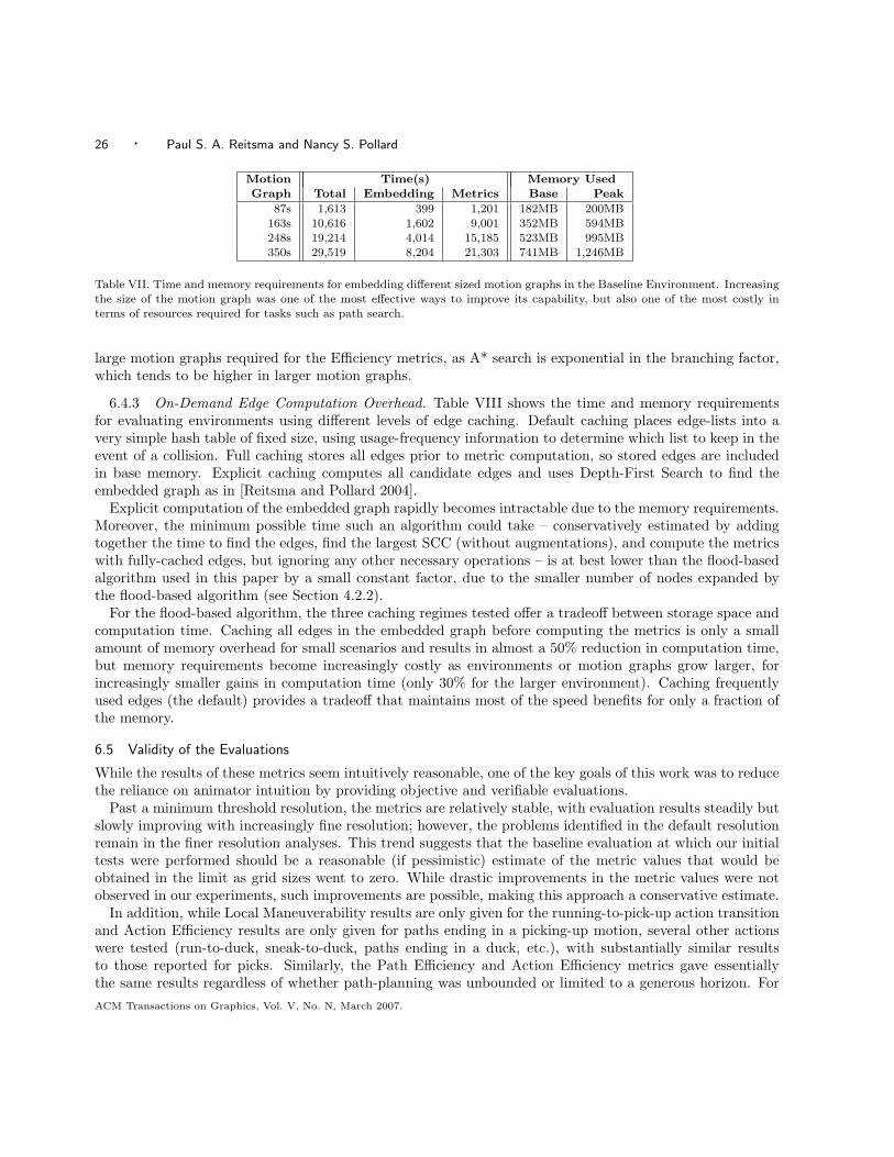
26 · Paul S. A. Reitsma and Nancy S. Pollard
Motion Time(s) Memory Used
Graph Total Embedding Metrics Base Peak
87s 1,613 399 1,201 182MB 200MB
163s 10,616 1,602 9,001 352MB 594MB248s 19,214 4,014 15,185 523MB 995MB
350s 29,519 8,204 21,303 741MB 1,246MB
Table VII. Time and memory requirements for embedding different sized motion graphs in the Baseline Environment. Increasingthe size of the motion graph was one of the most effective ways to improve its capability, but also one of the most costly in
terms of resources required for tasks such as path search.
large motion graphs required for the Efficiency metrics, as A* search is exponential in the branching factor,which tends to be higher in larger motion graphs.
6.4.3 On-Demand Edge Computation Overhead. Table VIII shows the time and memory requirementsfor evaluating environments using different levels of edge caching. Default caching places edge-lists into avery simple hash table of fixed size, using usage-frequency information to determine which list to keep in theevent of a collision. Full caching stores all edges prior to metric computation, so stored edges are includedin base memory. Explicit caching computes all candidate edges and uses Depth-First Search to find theembedded graph as in [Reitsma and Pollard 2004].
Explicit computation of the embedded graph rapidly becomes intractable due to the memory requirements.Moreover, the minimum possible time such an algorithm could take – conservatively estimated by addingtogether the time to find the edges, find the largest SCC (without augmentations), and compute the metricswith fully-cached edges, but ignoring any other necessary operations – is at best lower than the flood-basedalgorithm used in this paper by a small constant factor, due to the smaller number of nodes expanded bythe flood-based algorithm (see Section 4.2.2).
For the flood-based algorithm, the three caching regimes tested offer a tradeoff between storage space andcomputation time. Caching all edges in the embedded graph before computing the metrics is only a smallamount of memory overhead for small scenarios and results in almost a 50% reduction in computation time,but memory requirements become increasingly costly as environments or motion graphs grow larger, forincreasingly smaller gains in computation time (only 30% for the larger environment). Caching frequentlyused edges (the default) provides a tradeoff that maintains most of the speed benefits for only a fraction ofthe memory.
6.5 Validity of the Evaluations
While the results of these metrics seem intuitively reasonable, one of the key goals of this work was to reducethe reliance on animator intuition by providing objective and verifiable evaluations.
Past a minimum threshold resolution, the metrics are relatively stable, with evaluation results steadily butslowly improving with increasingly fine resolution; however, the problems identified in the default resolutionremain in the finer resolution analyses. This trend suggests that the baseline evaluation at which our initialtests were performed should be a reasonable (if pessimistic) estimate of the metric values that would beobtained in the limit as grid sizes went to zero. While drastic improvements in the metric values were notobserved in our experiments, such improvements are possible, making this approach a conservative estimate.
In addition, while Local Maneuverability results are only given for the running-to-pick-up action transitionand Action Efficiency results are only given for paths ending in a picking-up motion, several other actionswere tested (run-to-duck, sneak-to-duck, paths ending in a duck, etc.), with substantially similar resultsto those reported for picks. Similarly, the Path Efficiency and Action Efficiency metrics gave essentiallythe same results regardless of whether path-planning was unbounded or limited to a generous horizon. For
ACM Transactions on Graphics, Vol. V, No. N, March 2007.
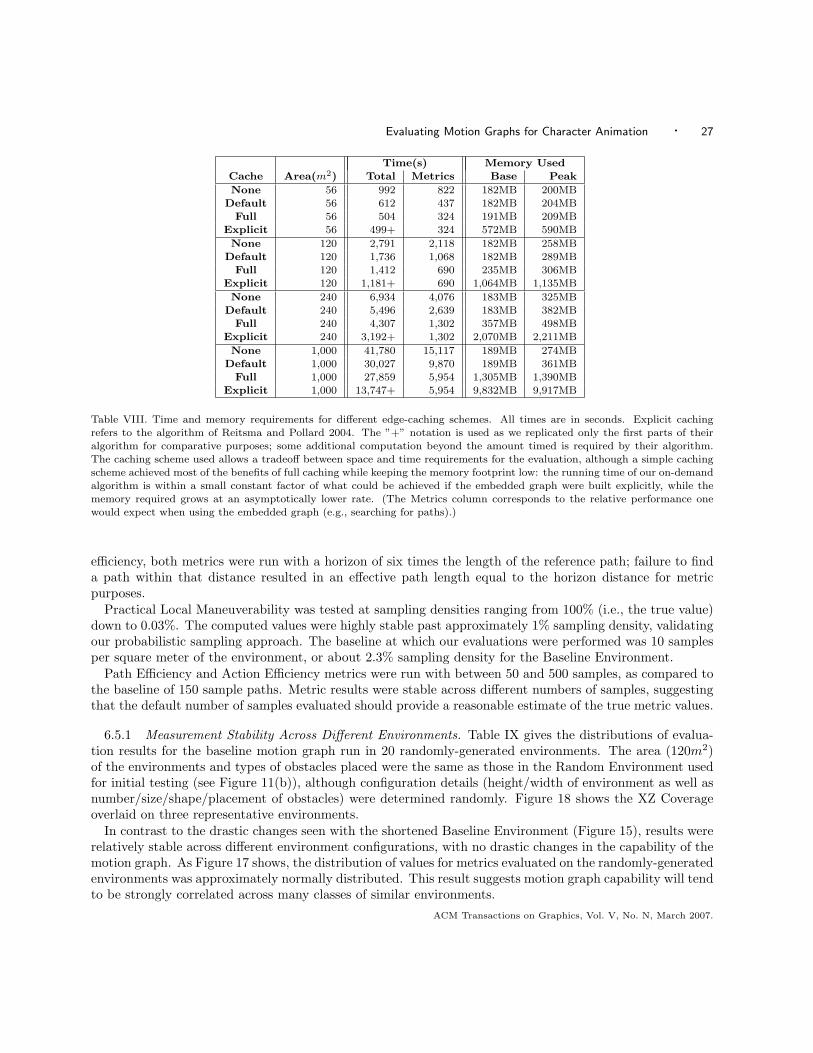
Evaluating Motion Graphs for Character Animation · 27
Time(s) Memory Used
Cache Area(m2) Total Metrics Base Peak
None 56 992 822 182MB 200MB
Default 56 612 437 182MB 204MBFull 56 504 324 191MB 209MB
Explicit 56 499+ 324 572MB 590MB
None 120 2,791 2,118 182MB 258MB
Default 120 1,736 1,068 182MB 289MB
Full 120 1,412 690 235MB 306MBExplicit 120 1,181+ 690 1,064MB 1,135MB
None 240 6,934 4,076 183MB 325MB
Default 240 5,496 2,639 183MB 382MB
Full 240 4,307 1,302 357MB 498MB
Explicit 240 3,192+ 1,302 2,070MB 2,211MB
None 1,000 41,780 15,117 189MB 274MB
Default 1,000 30,027 9,870 189MB 361MB
Full 1,000 27,859 5,954 1,305MB 1,390MB
Explicit 1,000 13,747+ 5,954 9,832MB 9,917MB
Table VIII. Time and memory requirements for different edge-caching schemes. All times are in seconds. Explicit cachingrefers to the algorithm of Reitsma and Pollard 2004. The ”+” notation is used as we replicated only the first parts of theiralgorithm for comparative purposes; some additional computation beyond the amount timed is required by their algorithm.
The caching scheme used allows a tradeoff between space and time requirements for the evaluation, although a simple cachingscheme achieved most of the benefits of full caching while keeping the memory footprint low: the running time of our on-demandalgorithm is within a small constant factor of what could be achieved if the embedded graph were built explicitly, while thememory required grows at an asymptotically lower rate. (The Metrics column corresponds to the relative performance one
would expect when using the embedded graph (e.g., searching for paths).)
efficiency, both metrics were run with a horizon of six times the length of the reference path; failure to finda path within that distance resulted in an effective path length equal to the horizon distance for metricpurposes.
Practical Local Maneuverability was tested at sampling densities ranging from 100% (i.e., the true value)down to 0.03%. The computed values were highly stable past approximately 1% sampling density, validatingour probabilistic sampling approach. The baseline at which our evaluations were performed was 10 samplesper square meter of the environment, or about 2.3% sampling density for the Baseline Environment.
Path Efficiency and Action Efficiency metrics were run with between 50 and 500 samples, as compared tothe baseline of 150 sample paths. Metric results were stable across different numbers of samples, suggestingthat the default number of samples evaluated should provide a reasonable estimate of the true metric values.
6.5.1 Measurement Stability Across Different Environments. Table IX gives the distributions of evalua-tion results for the baseline motion graph run in 20 randomly-generated environments. The area (120m2)of the environments and types of obstacles placed were the same as those in the Random Environment usedfor initial testing (see Figure 11(b)), although configuration details (height/width of environment as well asnumber/size/shape/placement of obstacles) were determined randomly. Figure 18 shows the XZ Coverageoverlaid on three representative environments.
In contrast to the drastic changes seen with the shortened Baseline Environment (Figure 15), results wererelatively stable across different environment configurations, with no drastic changes in the capability of themotion graph. As Figure 17 shows, the distribution of values for metrics evaluated on the randomly-generatedenvironments was approximately normally distributed. This result suggests motion graph capability will tendto be strongly correlated across many classes of similar environments.
ACM Transactions on Graphics, Vol. V, No. N, March 2007.

28 · Paul S. A. Reitsma and Nancy S. Pollard
Total Times(s) XZ Cvgs(%) Prac LM Path Efficiencies Action Efficiencies
Mean StdDev Mean StdDev Mean StdDev Mean StdDev Mean StdDev
1,535 260 90.3 3.1 5.8s 0.55s 1.25 0.11 2.11 0.36
Table IX. Mean values and standard deviations for evaluation results of randomly-generated environments. Environments with
similar types and densities of obstacles tend to induce similar levels of capability on motion graphs.
(a) XZ Coverage
(b) Action Efficiency
Fig. 17. Distributions of a representative pair of metric values for the random environments evaluated. Y axis is count ofnumber of environments in each bin. Metric values were distributed approximately normally.
7. DISCUSSION
7.1 Findings
When using regular motion graphs on general environments, our experiments identified several problems.
7.1.1 Effects of Complexity. One fundamental result of our experiments is the observation that whenworking with a motion graph data structure, easy tasks are easy; more complex tasks are hard. For a simpletask, such as basic locomotion in an obstacle-free environment, all motion graphs we tested performed well,
ACM Transactions on Graphics, Vol. V, No. N, March 2007.
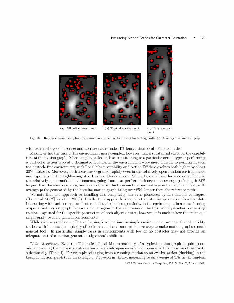
Evaluating Motion Graphs for Character Animation · 29
(a) Difficult environment (b) Typical environment (c) Easy environ-ment
Fig. 18. Representative examples of the random environments created for testing, with XZ Coverage displayed in grey.
with extremely good coverage and average paths under 1% longer than ideal reference paths.Making either the task or the environment more complex, however, had a substantial effect on the capabil-
ities of the motion graph. More complex tasks, such as transitioning to a particular action type or performinga particular action type at a designated location in the environment, were more difficult to perform in eventhe obstacle-free environment, with Local Maneuverability and Action Efficiency values both higher by about20% (Table I). Moreover, both measures degraded rapidly even in the relatively-open random environments,and especially in the highly-congested Baseline Environment. Similarly, even basic locomotion suffered inthe relatively-open random environments, going from near-perfect efficiency to an average path length 25%longer than the ideal reference, and locomotion in the Baseline Environment was extremely inefficient, withaverage paths generated by the baseline motion graph being over 85% longer than the reference paths.
We note that one approach to handling this complexity has been pioneered by Lee and his colleagues([Lee et al. 2002][Lee et al. 2006]). Briefly, their approach is to collect substantial quantities of motion datainteracting with each obstacle or cluster of obstacles in close proximity in the environment, in a sense forminga specialized motion graph for each unique region in the environment. As this technique relies on re-usingmotions captured for the specific parameters of each object cluster, however, it is unclear how the techniquemight apply to more general environments.
While motion graphs are effective for simple animations in simple environments, we note that the abilityto deal with increased complexity of both task and environment is necessary to make motion graphs a moregeneral tool. In particular, simple tasks in environments with few or no obstacles may not provide anadequate test of a motion generation algorithm’s abilities.
7.1.2 Reactivity. Even the Theoretical Local Maneuverability of a typical motion graph is quite poor,and embedding the motion graph in even a relatively open environment degrades this measure of reactivitysubstantially (Table I). For example, changing from a running motion to an evasive action (ducking) in thebaseline motion graph took an average of 3.6s even in theory, increasing to an average of 5.8s in the random
ACM Transactions on Graphics, Vol. V, No. N, March 2007.

30 · Paul S. A. Reitsma and Nancy S. Pollard
environments (Table IX) and 6.6s in the Baseline Environment. Considering that interactive environmentssuch as games and training scenarios will tend to operate at timescales driven by users’ recognition andchoice reaction times (approximately 0.5s, rising to 1s for unexpected stimuli; see [Green 2000a] [Green2000b] [Kosinski 2005]), substantial improvements in the ability of motion graphs to react to interactivecontrol are necessary. Ikemoto et al. [2006] examine one possible approach to this problem.
7.1.3 Embedding. We note the importance of evaluating the capability of a motion graph within thecontext of its target environment. Our experiments with variants of the Baseline Environment (Figure 15)show that minor changes to an environment can potentially cause drastic changes in the effective capabilityof one motion graph – in this case making the upper portion of the environment largely inaccessible – whilecausing virtually no changes in the effective capability of another motion graph. However, our experimentswith randomly-generated environments (Table IX) demonstrate that there is a strong correlation betweenthe capability of a motion graph in environments with similar types and densities of small obstacles. Thecapabilities of motion graphs in our randomly-generated environments were distributed approximately nor-mally (Figure 17). Based on the results with the Shortened Baseline Environment (Figure 15), however, itappears that smaller numbers of longer or wider obstacles will lead to less predictable capability than thelarger numbers of smaller obstacles used in the randomly-generated environments.
7.2 Identified Causes
Our experiments suggested three main problems with the motion graphs tested.
First, many clips, especially those of actions such as picking-up, ducking, or jumping, were effectively “setpieces” – i.e., they were linked into the motion graph in such a way that substantial amounts of specificmotion was unavoidable both before and after the action itself. Both instances of punching actions, forexample, required about eight meters of mostly straight-line movement to perform, resulting in the almostcomplete inability to perform punches in the Baseline Environment (Figure 14(c)). By contrast, other actionswere embedded in linear paths through the motion graph consisting of about 2-4m of movement, which wasmuch easier to place within the environment (Figure 14). Lengthy “set pieces” of motion such as theseare not only easily disrupted by obstacles, reducing the coverage of the action in the environment, but alsodrastically worsen Local Maneuverability.
Similarly, actions of these sorts tend to have only a few instances in the motion graph in order to keepthe overall size of the graph down as the variety of actions it contains increases. Unfortunately, the pathscorresponding to the instances of these actions are often poorly linked into the motion graph, with the startof the branchless portion of the path typically being accessible from very few (often only two) other clipsin the motion graph. In a congested environment, however, the ability to take any particular transitionfrom the character’s current location can easily be blocked by obstacles, meaning that the small numberof direct paths through the motion graph to the desired action can easily be rendered unavailable. Thismakes the character’s Local Maneuverability unacceptably fragile and variable, as well as contributing tothe inefficiency of paths.
Finally, many obstacles in close proximity, such as the lower-left region of the Baseline Environment (Figure11(c)), create a need for paths with specific patterns of left-and-right turning in order to wend between theobstacles. Motion graphs, due to their heavy reliance on the source data, have trouble substantially changingthe curvature patterns of their constituent paths, although some of this is possible during clip transitions.
We examined three common approaches to resolving these problems: adding more data to the basic motiongraph; allowing more extensive motion editing at clip transitions; and using a small but highly-connected,hub-based motion graph.
ACM Transactions on Graphics, Vol. V, No. N, March 2007.
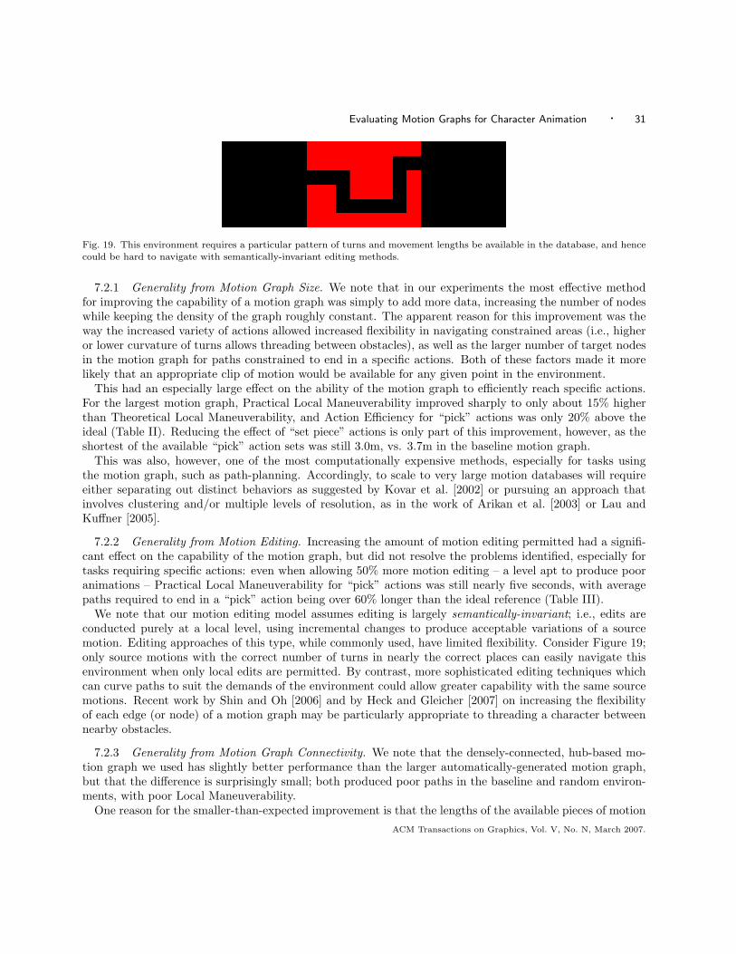
Evaluating Motion Graphs for Character Animation · 31
Fig. 19. This environment requires a particular pattern of turns and movement lengths be available in the database, and hencecould be hard to navigate with semantically-invariant editing methods.
7.2.1 Generality from Motion Graph Size. We note that in our experiments the most effective methodfor improving the capability of a motion graph was simply to add more data, increasing the number of nodeswhile keeping the density of the graph roughly constant. The apparent reason for this improvement was theway the increased variety of actions allowed increased flexibility in navigating constrained areas (i.e., higheror lower curvature of turns allows threading between obstacles), as well as the larger number of target nodesin the motion graph for paths constrained to end in a specific actions. Both of these factors made it morelikely that an appropriate clip of motion would be available for any given point in the environment.
This had an especially large effect on the ability of the motion graph to efficiently reach specific actions.For the largest motion graph, Practical Local Maneuverability improved sharply to only about 15% higherthan Theoretical Local Maneuverability, and Action Efficiency for “pick” actions was only 20% above theideal (Table II). Reducing the effect of “set piece” actions is only part of this improvement, however, as theshortest of the available “pick” action sets was still 3.0m, vs. 3.7m in the baseline motion graph.
This was also, however, one of the most computationally expensive methods, especially for tasks usingthe motion graph, such as path-planning. Accordingly, to scale to very large motion databases will requireeither separating out distinct behaviors as suggested by Kovar et al. [2002] or pursuing an approach thatinvolves clustering and/or multiple levels of resolution, as in the work of Arikan et al. [2003] or Lau andKuffner [2005].
7.2.2 Generality from Motion Editing. Increasing the amount of motion editing permitted had a signifi-cant effect on the capability of the motion graph, but did not resolve the problems identified, especially fortasks requiring specific actions: even when allowing 50% more motion editing – a level apt to produce pooranimations – Practical Local Maneuverability for “pick” actions was still nearly five seconds, with averagepaths required to end in a “pick” action being over 60% longer than the ideal reference (Table III).
We note that our motion editing model assumes editing is largely semantically-invariant; i.e., edits areconducted purely at a local level, using incremental changes to produce acceptable variations of a sourcemotion. Editing approaches of this type, while commonly used, have limited flexibility. Consider Figure 19;only source motions with the correct number of turns in nearly the correct places can easily navigate thisenvironment when only local edits are permitted. By contrast, more sophisticated editing techniques whichcan curve paths to suit the demands of the environment could allow greater capability with the same sourcemotions. Recent work by Shin and Oh [2006] and by Heck and Gleicher [2007] on increasing the flexibilityof each edge (or node) of a motion graph may be particularly appropriate to threading a character betweennearby obstacles.
7.2.3 Generality from Motion Graph Connectivity. We note that the densely-connected, hub-based mo-tion graph we used has slightly better performance than the larger automatically-generated motion graph,but that the difference is surprisingly small; both produced poor paths in the baseline and random environ-ments, with poor Local Maneuverability.
One reason for the smaller-than-expected improvement is that the lengths of the available pieces of motion
ACM Transactions on Graphics, Vol. V, No. N, March 2007.
32 · Paul S. A. Reitsma and Nancy S. Pollard
are not altered by this increased connectivity, and the character must often travel a significant distance beforereturning to a hub pose and becoming able to transition to a new clip of motion. For example, performinga “pick” action required playing approximately 3.7m of motion in the baseline motion graph before a choiceof which clip to transition to next was available, vs. 3.5m in the hub-based motion graph. Due to this,the immediate-horizon ability of the character to navigate through a congested environment is not greatlyimproved.
Accordingly, a highly-connected, hub-based motion graph which does not address the problem of long “setpiece” chunks of motion does not appear to adequately address the deficiencies observed.
One potential solution would be to increase the degree of connectivity not only at the ends of clips, butinside clips as well. This approach would allow the character to move between actions such as locomotionwith different radius of curvature more freely, permitting a greater ability to navigate in highly-congestedenvironments.
Unfortunately, this approach would substantially increase the size and density of the motion graph. Theresulting graph would be significantly harder to reason about, either intuitively or analytically, and wouldbe much more expensive to use for operations such as path planning. Both of these drawbacks underminesome of the important benefits of motion graphs, suggesting the importance of a careful and well-informedtradeoff.
7.3 Scaling Behavior
7.3.1 Memory. As noted in the theoretical analysis of memory requirements (Section 4.2.1), base memoryrequired increases linearly with the size of the target environment, but the constant is so small that theamount of memory required is not a bottleneck for our algorithm. The main component of base memoryis caching prerotated clips for faster edge computation; however, our results suggest that the overall basememory requirements are reasonable.
Peak memory requirements are driven by the A* search technique used to evaluate the ability of the motiongraph to produce efficient paths in the target environment. Due to the exponential nature of A*, this valueis highly sensitive to parameters such as the planning horizon, and in practice memory limitations can besignificantly lessened by appropriate parameter settings and heuristics. Moreover, applications using motiongraphs will by necessity already have a path-planning method in place, and that method will be the mostappropriate one to use when evaluating scenarios for that application. As such, peak memory requirementsand their solutions are amply discussed in the path-planning and search literature.
7.3.2 Computation Time. For larger and more complex scenarios, computation time is typically a strongerconcern than memory requirements. For larger environments, computation time is increasingly dominatedby the time required to embed the graph in the environment (increasing from under 30% for the smallestenvironment to over 60% for the largest). In practice, larger environments are often qualitatively differentfrom smaller environments, and their greater openness leads to denser embedded graphs.
By contrast, larger motion graphs continue to have the large part of their runtime (around 70%) comefrom path search. As with memory requirements, computational requirements for path search and pathplanning have been a subject of much research, and whatever method is intended for use in the applicationemploying the motion graph can be used efficiently in the embedded graph.
7.4 Alternative Editing Models
The analysis in this paper examined the capability of motion graphs constructed via a concatenation-basedapproach to motion editing (i.e., clips of source data are edited to fit together seamlessly, and are played oneafter another to animate the character). This approach typically uses displacement splines or blending (e.g.,[Kovar et al. 2002], [Stone et al. 2004], [Kwon and Shin 2005], [Lee et al. 2006], etc.), and can be augmented
ACM Transactions on Graphics, Vol. V, No. N, March 2007.
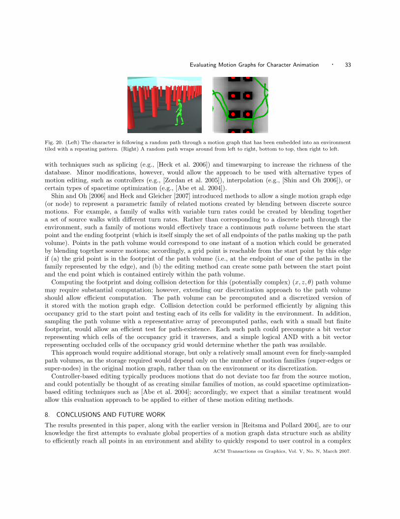
Evaluating Motion Graphs for Character Animation · 33
Fig. 20. (Left) The character is following a random path through a motion graph that has been embedded into an environmenttiled with a repeating pattern. (Right) A random path wraps around from left to right, bottom to top, then right to left.
with techniques such as splicing (e.g., [Heck et al. 2006]) and timewarping to increase the richness of thedatabase. Minor modifications, however, would allow the approach to be used with alternative types ofmotion editing, such as controllers (e.g., [Zordan et al. 2005]), interpolation (e.g., [Shin and Oh 2006]), orcertain types of spacetime optimization (e.g., [Abe et al. 2004]).
Shin and Oh [2006] and Heck and Gleicher [2007] introduced methods to allow a single motion graph edge(or node) to represent a parametric family of related motions created by blending between discrete sourcemotions. For example, a family of walks with variable turn rates could be created by blending togethera set of source walks with different turn rates. Rather than corresponding to a discrete path through theenvironment, such a family of motions would effectively trace a continuous path volume between the startpoint and the ending footprint (which is itself simply the set of all endpoints of the paths making up the pathvolume). Points in the path volume would correspond to one instant of a motion which could be generatedby blending together source motions; accordingly, a grid point is reachable from the start point by this edgeif (a) the grid point is in the footprint of the path volume (i.e., at the endpoint of one of the paths in thefamily represented by the edge), and (b) the editing method can create some path between the start pointand the end point which is contained entirely within the path volume.
Computing the footprint and doing collision detection for this (potentially complex) (x, z, θ) path volumemay require substantial computation; however, extending our discretization approach to the path volumeshould allow efficient computation. The path volume can be precomputed and a discretized version ofit stored with the motion graph edge. Collision detection could be performed efficiently by aligning thisoccupancy grid to the start point and testing each of its cells for validity in the environment. In addition,sampling the path volume with a representative array of precomputed paths, each with a small but finitefootprint, would allow an efficient test for path-existence. Each such path could precompute a bit vectorrepresenting which cells of the occupancy grid it traverses, and a simple logical AND with a bit vectorrepresenting occluded cells of the occupancy grid would determine whether the path was available.
This approach would require additional storage, but only a relatively small amount even for finely-sampledpath volumes, as the storage required would depend only on the number of motion families (super-edges orsuper-nodes) in the original motion graph, rather than on the environment or its discretization.
Controller-based editing typically produces motions that do not deviate too far from the source motion,and could potentially be thought of as creating similar families of motion, as could spacetime optimization-based editing techniques such as [Abe et al. 2004]; accordingly, we expect that a similar treatment wouldallow this evaluation approach to be applied to either of these motion editing methods.
8. CONCLUSIONS AND FUTURE WORK
The results presented in this paper, along with the earlier version in [Reitsma and Pollard 2004], are to ourknowledge the first attempts to evaluate global properties of a motion graph data structure such as abilityto efficiently reach all points in an environment and ability to quickly respond to user control in a complex
ACM Transactions on Graphics, Vol. V, No. N, March 2007.

34 · Paul S. A. Reitsma and Nancy S. Pollard
Fig. 21. Increasing the size of a motion graph improves capability for all tasks, but different metrics approach their optimalvalue at different rates. The Y axis shows how close a particular metric is to its ideal value, while the X axis shows the sizeof the motion graph (approximately 100, 200, 300, or 400 clips). Simpler tasks, such as efficient navigation (“Path”, pink line)
approach optimal more rapidly than more complex tasks, such as efficiently picking up an object at a specified location (“Pick”,yellow line), suggesting that past a certain size it may be most useful to ignore the unconstrained navigation task and insteadtarget added clips towards improving the picking task. By contrast, tasks such as rapid response to user input (Practical LocalManeuverability or “LMP”, blue line) are not improved to near their optimal level by to this improvement method, suggesting
that a radically different method, or even an algorithmic change, may be necessary.
environment.Embedding a motion graph into the environment and assessing global properties of this data structure
allows us to compare motion datasets and identify weak points in these motion datasets and problematicareas in the environments. In addition, analysis of a range of motion graphs across a range of environmentscan shed light on the strengths and weaknesses of the motion graph algorithm in general.
We also provide a method for determining a reasonable answer to the standard question of “how muchmotion is enough?” Our analysis techniques, coupled with task-based metrics representing the application athand, can be used to evaluate the capabilities of a motion graph, allowing one to be selected that is neithertoo big for efficient searching and planning nor too small for effective task performance.
Our experiments highlighted several important considerations regarding generating animations with mo-tion graphs.
First, capability degrades surprisingly rapidly with increasing complexity. Tasks more complex than basicnavigation and environments with obstacles in close proximity sharply narrow the options available whenpath-planning with a motion graph. Accordingly, testing an animation system with only simple tasks orrelatively unconstrained environments may not provide the full picture of the system’s abilities.
Reactivity for characters animated by motion graphs is often poor even in theory, and is easily degradedfurther by complex tasks or environments. The ability to react rapidly to user control, however, is crucialto interactive applications, and an inability to move efficiently between motion types lessens the capabilityof motion graphs with regards to more complex tasks.
Several approaches can help alleviate these problems, including denser motion graphs (perhaps with shorterclips or edges transitioning from the inside of clips), more sophisticated editing techniques, and adding moredata to motion graphs. These approaches tend to offer performance tradeoffs, however, increasing capabilitywhile increasing the computational cost of using a motion graph.
ACM Transactions on Graphics, Vol. V, No. N, March 2007.
Evaluating Motion Graphs for Character Animation · 35
Our hope is that analysis methods such as the one in this paper will be useful in managing tradeoffs suchas these. For example, our analysis revealed that the motion graph improvement methods tended to improvethe different metrics at different rates (Figure 21). One potential application of these methods is to directavailable memory or computation resources towards those tasks which will generate the greatest capabilitybang for the resource buck.
In addition, such methods potentially allow a motion graph to be certified as sufficient for a particularenvironment and set of tasks, or even certified as suitable for a class of environments (e.g., environmentswhose obstacles do not cluster more tightly than a certain threshold). Additionally, a conservative estima-tion of capability may allow deemed-acceptable motion graphs to be used with confidence in their targetenvironments.
We see several directions for extensions to this research. A more general scenario could include dynamicenvironments, multiple autonomous characters, deformable objects, and complex interactions, and we hope torelax some of the simplifying assumptions we have made about the nature of the scenario to be evaluated. Inaddition, this evaluation approach could be placed in a feedback loop with a motion graph generation system,potentially allowing automatic optimization of motion graphs. As well, we are interested in generalizing theevaluation approach, both to other task domains and to other motion generation algorithms.
Finally, we note that the main bottleneck in the current approach is computation time. One optionfor reducing this time is to divide the environment into segments, either examining only those segmentsrequired (such as in the case of localized changes to obstacles) or forming the environment out of a numberof repeatable tiles (see Figure 20; this approach is examined in more detail in [Reitsma and Pollard 2004]and [Lee et al. 2006]). Alternatively, it should be noted that all major steps in the evaluation process arehighly parallelizeable, allowing a tradeoff between computation time and required hardware.
In summary, the techniques shown here provide a way to evaluate a character’s capabilities that is moresound than the trial and error approach commonly used. Evaluation techniques such as these can help auser to compare alternative data structures and provide detailed information on performance to aid the userin refining their motion graph or motion generation algorithm.
ACKNOWLEDGMENTS
Supported in part by the NSF under grants IIS-0326322, CCF-0343161, and ECS-0325383. Alias/Wavefrontdonated their Maya software for use in this research.
A. EDITING FOOTPRINTS
The editing model is based on the intuition that the amount a motion can be changed will tend to grow withthe distance it covers, as well as with the time spanned by the clip—in essence, we assume an error will beacceptably small if it is small relative to the rate at which other actions are taking place.
We specify the amount that V , the root position and orientation, can be adjusted as a linear function ofboth distance traveled and number of frames in the clip:
abs (Vi − V ′) < (s + αd)
rx
rz
rθ
(15)
where (Vi − V ′) is the vector difference between the new and original root configurations, s is the arclengthof the original motion clip, d is the duration of the motion clip, α is a scaling factor used to weight arc lengthvs. duration in terms of editing importance, and (s + αd)[rx rz rθ]
T is the size of the ellipsoidal footprintrepresenting allowable edits to root configuration.
The new path taken by the clip is computed by adding the currently-accumulated portion of (Vi − V ′) to
ACM Transactions on Graphics, Vol. V, No. N, March 2007.
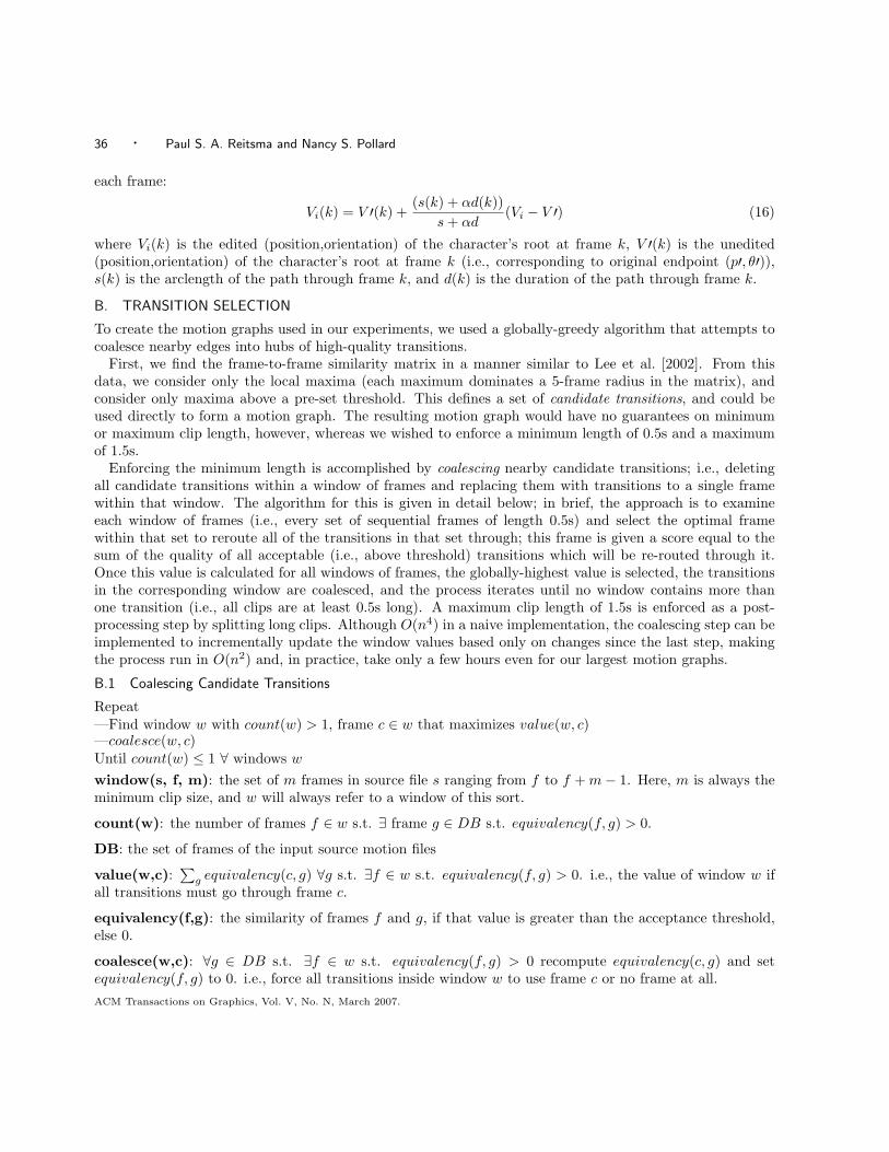
36 · Paul S. A. Reitsma and Nancy S. Pollard
each frame:
Vi(k) = V ′(k) +(s(k) + αd(k))
s + αd(Vi − V ′) (16)
where Vi(k) is the edited (position,orientation) of the character’s root at frame k, V ′(k) is the unedited(position,orientation) of the character’s root at frame k (i.e., corresponding to original endpoint (p′, θ′)),s(k) is the arclength of the path through frame k, and d(k) is the duration of the path through frame k.
B. TRANSITION SELECTION
To create the motion graphs used in our experiments, we used a globally-greedy algorithm that attempts tocoalesce nearby edges into hubs of high-quality transitions.
First, we find the frame-to-frame similarity matrix in a manner similar to Lee et al. [2002]. From thisdata, we consider only the local maxima (each maximum dominates a 5-frame radius in the matrix), andconsider only maxima above a pre-set threshold. This defines a set of candidate transitions, and could beused directly to form a motion graph. The resulting motion graph would have no guarantees on minimumor maximum clip length, however, whereas we wished to enforce a minimum length of 0.5s and a maximumof 1.5s.
Enforcing the minimum length is accomplished by coalescing nearby candidate transitions; i.e., deletingall candidate transitions within a window of frames and replacing them with transitions to a single framewithin that window. The algorithm for this is given in detail below; in brief, the approach is to examineeach window of frames (i.e., every set of sequential frames of length 0.5s) and select the optimal framewithin that set to reroute all of the transitions in that set through; this frame is given a score equal to thesum of the quality of all acceptable (i.e., above threshold) transitions which will be re-routed through it.Once this value is calculated for all windows of frames, the globally-highest value is selected, the transitionsin the corresponding window are coalesced, and the process iterates until no window contains more thanone transition (i.e., all clips are at least 0.5s long). A maximum clip length of 1.5s is enforced as a post-processing step by splitting long clips. Although O(n4) in a naive implementation, the coalescing step can beimplemented to incrementally update the window values based only on changes since the last step, makingthe process run in O(n2) and, in practice, take only a few hours even for our largest motion graphs.
B.1 Coalescing Candidate Transitions
Repeat—Find window w with count(w) > 1, frame c ∈ w that maximizes value(w, c)—coalesce(w, c)Until count(w) ≤ 1 ∀ windows w
window(s, f, m): the set of m frames in source file s ranging from f to f + m − 1. Here, m is always theminimum clip size, and w will always refer to a window of this sort.
count(w): the number of frames f ∈ w s.t. ∃ frame g ∈ DB s.t. equivalency(f, g) > 0.
DB: the set of frames of the input source motion files
value(w,c):∑
g equivalency(c, g) ∀g s.t. ∃f ∈ w s.t. equivalency(f, g) > 0. i.e., the value of window w ifall transitions must go through frame c.
equivalency(f,g): the similarity of frames f and g, if that value is greater than the acceptance threshold,else 0.
coalesce(w,c): ∀g ∈ DB s.t. ∃f ∈ w s.t. equivalency(f, g) > 0 recompute equivalency(c, g) and setequivalency(f, g) to 0. i.e., force all transitions inside window w to use frame c or no frame at all.
ACM Transactions on Graphics, Vol. V, No. N, March 2007.

Evaluating Motion Graphs for Character Animation · 37
Motion Graph
Clips Transitions Motion
98 288 87s
190 904 163s282 1,712 248s
389 3,198 350s
Table X. Clips, transitions, and total amount of motion contained by the different motion graphs created for our main evalua-tions. The full motion database contained 439 seconds of motion.
B.2 Crafting Representative Motion Graphs
The frame-to-frame similarity matrix computed above will depend strongly on the precise details of theinput motion capture clips. In practice, even a relatively small change in the transition qualities between aninput file and other files in the database can result in a substantially different motion graph. If one runningmotion is replaced by another, for example, or even if the same running motion is used but with a differenttransition-selection threshold, a very different motion graph can result due to the discrete nature of takinglocal maxima in the similarity matrix, coalescing them to enforce minimum clip lengths, and taking thelargest strongly connected component of the result.
In order to ensure that high-quality and representative motion graphs were used for our tests, each ofthe 50 input files was assigned a “desirability” weight which directly modified the relative quality of anytransitions to or from that motion. These weights were manually adjusted until an acceptable motion graphwas obtained. Our baseline motion graph was crafted via these weights to have a representative mix of allavailable motion types, with an emphasis on the two main locomotions (running and sneaking), a smalleramount of idling motion, and one to four examples of each of the actions (jumping, picking-up, ducking,punching, kicking) in the database. In addition, we ensured that each instance of an action was directlyaccessible from locomotion (i.e., it was not necessary to pass through a kicking motion to reach a duckingmotion, for example), and that all three types of locomotion (including idling) could be reached from eachother without passing through an action clip (i.e., the motion graph consisting of just the three locomotionswas also a strongly connected component).
Three larger motion graphs were created from the primary motion database in the manner detailed above(see Table X). The sneaking and running motions contained in the baseline motion graph created by thisprocess is visualized in Figure 22.
REFERENCES
Abe, Y., Liu, C. K., and Popovic, Z. 2004. Momentum-based parameterization of dynamic character motion. In 2004 ACMSIGGRAPH / Eurographics Symposium on Computer Animation. 173–182.
Arikan, O. and Forsyth, D. A. 2002. Interactive motion generation from examples. ACM Transactions on Graphics 21, 3(July), 483–490.
Arikan, O., Forsyth, D. A., and O’Brien, J. F. 2003. Motion synthesis from annotations. ACM Transactions on Graph-ics 22, 3 (July), 402–408.
Aubin, J.-P. 1990. A survey of viability theory. Society for Industrial and Applied Mathematics Journal of Control andOptimization, 28(4), p.749-788 .
Choi, M. G., Lee, J., and Shin, S. Y. 2003. Planning biped locomotion using motion capture data and probabilistic roadmaps.
ACM Transactions on Graphics 22, 2 (Apr.), 182–203.
Donald, B., Xavier, P., Canny, J., and Reif, J. 1993. Kinodynamic motion planning. Journal of the ACM 40, 5, 1048–1066.
Gleicher, M., Shin, H. J., Kovar, L., and Jepsen, A. 2003. Snap-together motion: Assembling run-time animation. ACMTransactions on Graphics 22, 3 (July), 702–702.
Gottschalk, S., Lin, M. C., and Manocha, D. 1996. OBBTree: A hierarchical structure for rapid interference detection.Computer Graphics 30, Annual Conference Series, 171–180.
ACM Transactions on Graphics, Vol. V, No. N, March 2007.

38 · Paul S. A. Reitsma and Nancy S. Pollard
(a) Paths (4x4m) (b) Depth 1 (11x11m) (c) Depth 2 (11x11m) (d) Depth 3 (11x11m)
Fig. 22. Figure 22(a) shows the sneaking and running motions available in the Baseline motion graph, displayed in a 4m by 4marea. The character starts at the white dot, facing upwards. The other figures show in an 11m by 11m area all available sneakingand running motions unrolled to different depths of graph expansion, along with additional clips representing discretized sampleof the result of applying our editing model to those source motions. Endpoint markers (green) mark the extent of each clip’s
editing footprint.
Green, M. 2000a. Driver reaction time. http://www.visualexpert.com/Resources/reactiontime.html .
Green, M. 2000b. How long does it take to stop? methodological analysis of driver perception-brake times. TransportationHuman Factors, 2(3), 195-216 .
Harrison, J., Rensink, R. A., and van de Panne, M. 2004. Obscuring length changes during animated motion. ACM
Transactions on Graphics 23, 3 (Aug.), 569–573.
Heck, R. and Gleicher, M. 2007. Parametric motion graphs. In 2007 ACM Symposium on Interactive 3D Graphics.
Heck, R., Kovar, L., and Gleicher, M. 2006. Splicing upper-body actions with locomotion. Computer Graphics Forum 25, 3
(Sept.), 459–466.
Hodgins, J. K., O’Brien, J. F., and Tumblin, J. 1998. Perception of human motion with different geometric models. IEEETransactions on Visualization and Computer Graphics 4, 4 (October), 307–316.
hoon Kim, T., Park, S. I., and Shin, S. Y. 2003. Rhythmic-motion synthesis based on motion-beat analysis. ACM Transactions
on Graphics 22, 3 (July), 392–401.
Ikemoto, L. K. M., Arikan, O., and Forsyth, D. 2006. Quick motion transitions with cached multi-way blends. Tech. Rep.UCB/EECS-2006-14, EECS Department, University of California, Berkeley. February 13.
Kavraki, L. E. and Latombe, J.-C. 1998. Probabilistic roadmaps for robot path planning. In Practical Motion Planning InRobotics: Current Approaches and Future Directions, K. Gupta and A. del Pobil, Eds. John Wiley, 33–53.
Kosinski, R. J. 2005. A literature review on reaction time. http://biae.clemson.edu/bpc/bp/Lab/110/reaction.htm.
Kovar, L., Gleicher, M., and Pighin, F. 2002. Motion graphs. ACM Transactions on Graphics 21, 3 (July), 473–482.
Kwon, T. and Shin, S. Y. 2005. Motion modeling for on-line locomotion synthesis. In 2005 ACM SIGGRAPH / EurographicsSymposium on Computer Animation. 29–38.
Latombe, J. C. 1991. Robot Motion Planning. Kluwer Academic Publishers, Boston.
Lau, M. and Kuffner, J. J. 2005. Behavior planning for character animation. In 2005 ACM SIGGRAPH / EurographicsSymposium on Computer Animation. 271–280.
Lee, J., Chai, J., Reitsma, P. S. A., Hodgins, J. K., and Pollard, N. S. 2002. Interactive control of avatars animated withhuman motion data. ACM Transactions on Graphics 21, 3 (July), 491–500.
Lee, K. H., Choi, M. G., and Lee, J. 2006. Motion patches: building blocks for virtual environments annotated with motiondata. ACM Transactions on Graphics 25, 3 (July), 898–906.
Li, Y., Wang, T., and Shum, H.-Y. 2002. Motion texture: A two-level statistical model for character motion synthesis. ACMTransactions on Graphics 21, 3 (July), 465–472.
Lozano-Perez, T. and O’Donnell, P. A. 1991. Parallel robot motion planning. In Proc. IEEE Intl. Conference on Roboticsand Automation.
Luenberger, D. G. 1979. Introduction to Dynamic Systems: Theory, Models, and Applications. John Wiley & Sons.
Mizuguchi, M., Buchanan, J., and Calvert, T. 2001. Data driven motion transitions for interactive games. In ShortPresentation, Eurographics 2001.
ACM Transactions on Graphics, Vol. V, No. N, March 2007.

Evaluating Motion Graphs for Character Animation · 39
Molina-Tanco, L. and Hilton, A. 2000. Realistic synthesis of novel human movements from a database of motion capture
examples. In In proceedings of IEEE Workshop on Human Motion 2000.
Muthukrishnan, S. and Pandurangan, G. 2005. The bin-covering technique for thresholding random geometric graph
properties. In Proceedings of SODA 2005.
Oesker, M., Hecht, H., and Jung, B. 2000. Psychological evidence for unconscious processing of detail in real-time animation
of multiple characters. Journal of Visualization and Computer Animation 11, 105–112.
Reitsma, P. S. A. and Pollard, N. S. 2003. Perceptual metrics for character animation: Sensitivity to errors in ballisticmotion. ACM Transactions on Graphics 22, 3 (July), 537–542.
Reitsma, P. S. A. and Pollard, N. S. 2004. Evaluating motion graphs for character navigation. In 2004 ACM SIGGRAPH/ Eurographics Symposium on Computer Animation. 89–98.
Ren, L., Patrick, A., Efros, A. A., Hodgins, J. K., and Rehg, J. M. 2005. A data-driven approach to quantifying naturalhuman motion. ACM Transactions on Graphics 24, 3 (Aug.), 1090–1097.
Safonova, A. and Hodgins, J. K. 2005. Analyzing the physical correctness of interpolated human motion. In 2005 ACMSIGGRAPH / Eurographics Symposium on Computer Animation. 171–180.
Shin, H. J. and Oh, H. S. 2006. Fat graphs: Constructing an interactive character with continuous controls. In 2006 ACMSIGGRAPH / Eurographics Symposium on Computer Animation. 291–298.
Stone, M., DeCarlo, D., Oh, I., Rodriguez, C., Stere, A., Lees, A., and Bregler, C. 2004. Speaking with hands: creatinganimated conversational characters from recordings of human performance. ACM Transactions on Graphics 23, 3 (Aug.),
506–513.
Sung, M., Kovar, L., and Gleicher, M. 2005. Fast and accurate goal-directed motion synthesis for crowds. In 2005 ACM
SIGGRAPH / Eurographics Symposium on Computer Animation. 291–300.
Suthankar, G., Mandel, M., Sycara, K., and Hodgins, J. K. 2004. Modeling physical capabilities of humanoid agents using
motion capture. In AAMAS 2004 Proceedings.
Wang, J. and Bodenheimer, B. 2003. An evaluation of a cost metric for selecting transitions between motion segments. In
2003 ACM SIGGRAPH / Eurographics Symposium on Computer Animation. 232–238.
Wang, J. and Bodenheimer, B. 2004. Computing the duration of motion transitions: an empirical approach. In 2004 ACM
SIGGRAPH / Eurographics Symposium on Computer Animation. 335–344.
Zordan, V. B., Majkowska, A., Chiu, B., and Fast, M. 2005. Dynamic response for motion capture animation. ACM
Transactions on Graphics 24, 3 (Aug.), 697–701.
Received Month Year Revised Month Year Accepted Month Year
ACM Transactions on Graphics, Vol. V, No. N, March 2007.


![Hybrid Motion Graphs for Character Animation€¦ · fewer paths will become available [7]. Yazhou [8] proposes a locomotion planner based motion graphs coupling with an upper-body](https://static.fdocuments.in/doc/165x107/5f8d6518613b3b232e22db48/hybrid-motion-graphs-for-character-animation-fewer-paths-will-become-available-7.jpg)