Evaluating Model Estimation Processes for Diagnostic ...
127
Evaluating Model Estimation Processes for Diagnostic Classification Models By W. Jake Thompson Submitted to the graduate degree program in Educational Psychology and the Graduate Faculty of the University of Kansas in partial fulfillment of the requirements for the degree of Doctor of Philosophy. Committee members Neal Kingston, PhD, Chairperson Jonathan Templin, PhD William Skorupski, PhD Brooke Nash, PhD Paul Johnson, PhD, Outside member Date defended: March 28, 2018
Transcript of Evaluating Model Estimation Processes for Diagnostic ...
Evaluating Model Estimation Processes for DiagnosticClassification Models
By
W. Jake Thompson
Submitted to the graduate degree program in Educational Psychology and the Graduate Faculty ofthe University of Kansas in partial fulfillment of the requirements for the degree of Doctor of
Philosophy.
Committee members
Neal Kingston, PhD, Chairperson
Jonathan Templin, PhD
William Skorupski, PhD
Brooke Nash, PhD
Paul Johnson, PhD, Outside member
Date defended: March 28, 2018
The Dissertation Committee for W. Jake Thompson certifiesthat this is the approved version of the following dissertation:
Evaluating Model Estimation Processes for Diagnostic Classification Models
Neal Kingston, PhD, Chairperson
Date approved: March 28, 2018
ii
Abstract
Diagnostic classification models (DCMs) are a class of models that define respondent
ability on a set of predefined categorical latent variables. In recent years, the pop-
ularity of these models has begun to increase. As the community of researchers of
practitioners of DCMs grow, it is important to examine the implementation of these
models, including the process of model estimation. A key aspect of the estimation
process that remains unexplored in the DCM literature is model reduction, or the re-
moval of parameters from the model in order to create a simpler, more parsimonious
model. The current study fills this gap in the literature by first applying several model
reduction processes on a real data set, the Diagnosing Teachers’ Multiplicative Rea-
soning assessment (Bradshaw et al., 2014). Results from this analysis indicate that the
selection of model reduction process can have large implications for the resulting pa-
rameter estimates and respondent classifications. A simulation study is then conducted
to evaluate the relative performance of these various model reduction processes. The
results of the simulation suggest that all model reduction processes are able to provide
quality estimates of the item parameters and respondent masteries, if the model is able
to converge. The findings also show that if the full model does not converge, then re-
ducing the structural model provides the best opportunities for achieving a converged
solution. Implications of this study and directions for future research are discussed.
Keywords. Diagnostic classification models, log-linear cognitive diagnosis model,
model reduction, Monte Carlo simulation
iii

Acknowledgements
I would like to thank my advisor, Neal Kingston, for his mentorship, guidance, support, and limit-
less optimism. I’ve been extremely lucky to have an advisor that has opened the door to so many
opportunities for me to grow. Thank you for teaching me to always strive for the ideal, rather than
settling for what seems possible at the time.
I would also like to thank the rest of my committee: Jonathan Templin, Billy Skorupski, Paul
Johnson, and Brooke Nash. Jonathan, thank you for introducing me to diagnostic models and
sharing your knowledge with me. I am incredibly appreciative for all the time you have spent
answering my questions, not just about DCMs, but also sports models and any other project I
email you about. Billy, thank you for teaching me how to think about psychometrics. Without
your guidance and willingness to share your expertise I would not be the psychometrician I am
today. Paul, thank you for teaching me how to be a better programmer and software developer.
This simulation study would not have been nearly as efficient without your guidance. Brooke,
thank you for keeping me grounded in the real-world impact of my work when I start to get too
high in the ivory tower. Thank you also for constantly being a sounding board for me to talk
through issues with as I take over your white board.
I am also thankful to Accessible Teaching, Learning, and Assessment Systems for financial
and computing resources that supported this project. Even more so, I am thankful to the rest of
the Dynamic Learning Maps psychometric, specifically Amy Clark and Meagan Karvonen, for the
mentorship and support that has contributed to both my professional and personal growth.
None of this would have been possible without my family who have provided nonstop encour-
agement and support. I would not be who I am today without my parents’ unquestioning belief
in me. I am so very grateful for the seemingly unending amount of patience they have given me
during my years in graduate school in addition to their unconditional love and support. I promise
iv

to call and visit more!
I also must thank my Kansas City family and friends. To my in-laws, thank you for welcoming
me into your family and your home, taking care of Larry when our schedules get busy, and always
giving me a laugh and a distraction. Thank you also to my close friend and former cube-mate
Jennifer Brussow, who is always ready to talk through any issue or question that pops into my
head, no matter the subject. And to my dog Larry, who can’t read this but spent many late nights
and early mornings on the couch with me as I worked on this project: thank you for filling my life
with warm snuggles, breadsticks, and cold licks.
Finally, I would like to thank my wonderful wife Julia. Without you none of this would have
been possible. Out of everything I’m thankful for, you are by far the top of the list. Thank you for
always supporting me and listening to me rant about my latest programming challenges. This is as
much your accomplishment as it is mine. Thank you for everything. I love you!
v
Contents
1 Introduction 1
1.1 Study constraints . . . . . . . . . . . . . . . . . . . . . . . . . . . . . . . . . . . 2
1.2 Colophon . . . . . . . . . . . . . . . . . . . . . . . . . . . . . . . . . . . . . . . 3
2 Literature Review 4
2.1 Structure of diagnostic classification models . . . . . . . . . . . . . . . . . . . . . 5
2.1.1 The Q-matrix . . . . . . . . . . . . . . . . . . . . . . . . . . . . . . . . . 7
2.2 Types of DCMs . . . . . . . . . . . . . . . . . . . . . . . . . . . . . . . . . . . . 8
2.2.1 Noncompensatory DCMs . . . . . . . . . . . . . . . . . . . . . . . . . . . 8
2.2.2 Compensatory DCMs . . . . . . . . . . . . . . . . . . . . . . . . . . . . 9
2.3 The log-linear cognitive diagnosis model . . . . . . . . . . . . . . . . . . . . . . . 10
2.3.1 LCDM measurement model . . . . . . . . . . . . . . . . . . . . . . . . . 11
2.4 Structural models . . . . . . . . . . . . . . . . . . . . . . . . . . . . . . . . . . . 15
2.4.1 Log-linear structural models . . . . . . . . . . . . . . . . . . . . . . . . . 16
2.5 Model reduction . . . . . . . . . . . . . . . . . . . . . . . . . . . . . . . . . . . . 17
2.5.1 Model reduction in structural equation modeling . . . . . . . . . . . . . . 18
2.5.2 Model reduction in item response theory . . . . . . . . . . . . . . . . . . . 19
2.5.3 Model reduction in DCMs . . . . . . . . . . . . . . . . . . . . . . . . . . 20
2.6 The current study . . . . . . . . . . . . . . . . . . . . . . . . . . . . . . . . . . . 21
3 Pilot Study 23
3.1 Method . . . . . . . . . . . . . . . . . . . . . . . . . . . . . . . . . . . . . . . . 23
3.1.1 DTMR data . . . . . . . . . . . . . . . . . . . . . . . . . . . . . . . . . . 23
vi
3.1.2 Model estimation . . . . . . . . . . . . . . . . . . . . . . . . . . . . . . . 25
3.2 Results . . . . . . . . . . . . . . . . . . . . . . . . . . . . . . . . . . . . . . . . . 27
3.2.1 Measurement model results . . . . . . . . . . . . . . . . . . . . . . . . . 27
3.2.2 Structural model results . . . . . . . . . . . . . . . . . . . . . . . . . . . 32
3.3 Conclusions . . . . . . . . . . . . . . . . . . . . . . . . . . . . . . . . . . . . . . 34
4 Methods 36
4.1 Overview of Monte Carlo methods . . . . . . . . . . . . . . . . . . . . . . . . . . 36
4.2 The current simulation . . . . . . . . . . . . . . . . . . . . . . . . . . . . . . . . 37
4.2.1 Simulation conditions . . . . . . . . . . . . . . . . . . . . . . . . . . . . 37
4.2.2 Data generation process . . . . . . . . . . . . . . . . . . . . . . . . . . . 38
4.2.3 Model reduction process . . . . . . . . . . . . . . . . . . . . . . . . . . . 39
4.2.4 Outcome measures . . . . . . . . . . . . . . . . . . . . . . . . . . . . . . 41
4.2.5 Software . . . . . . . . . . . . . . . . . . . . . . . . . . . . . . . . . . . 42
5 Results 43
5.1 Reduction by p-value . . . . . . . . . . . . . . . . . . . . . . . . . . . . . . . . . 44
5.1.1 Convergence . . . . . . . . . . . . . . . . . . . . . . . . . . . . . . . . . 44
5.1.2 Parameter recovery . . . . . . . . . . . . . . . . . . . . . . . . . . . . . . 45
5.1.3 Mastery classification . . . . . . . . . . . . . . . . . . . . . . . . . . . . . 49
5.1.4 Model fit . . . . . . . . . . . . . . . . . . . . . . . . . . . . . . . . . . . 53
5.1.5 Description of reduced parameters . . . . . . . . . . . . . . . . . . . . . . 56
5.2 Reduction by heuristic . . . . . . . . . . . . . . . . . . . . . . . . . . . . . . . . 61
5.2.1 Convergence . . . . . . . . . . . . . . . . . . . . . . . . . . . . . . . . . 62
5.2.2 Parameter recovery . . . . . . . . . . . . . . . . . . . . . . . . . . . . . . 64
5.2.3 Mastery classification . . . . . . . . . . . . . . . . . . . . . . . . . . . . . 67
5.2.4 Model fit . . . . . . . . . . . . . . . . . . . . . . . . . . . . . . . . . . . 71
5.2.5 Description of reduced parameters . . . . . . . . . . . . . . . . . . . . . . 74
vii
6 Conclusions 78
6.1 Limitations and future directions . . . . . . . . . . . . . . . . . . . . . . . . . . . 80
References 82
A Parameter Recovery with Reduction from P-values 91
A.1 Individual Bias . . . . . . . . . . . . . . . . . . . . . . . . . . . . . . . . . . . . 91
A.2 Individual Mean Square Error . . . . . . . . . . . . . . . . . . . . . . . . . . . . 97
B Parameter Recovery with Reduction from Heuristic 103
B.1 Individual Bias . . . . . . . . . . . . . . . . . . . . . . . . . . . . . . . . . . . . 103
B.2 Individual Mean Square Error . . . . . . . . . . . . . . . . . . . . . . . . . . . . 109
viii
List of Figures
3.1 Flowchart of model reduction processes . . . . . . . . . . . . . . . . . . . . . . . 26
3.2 DTMR respondent classification under each model reduction process . . . . . . . . 34
4.1 Flowchart of simulation study reduction processes . . . . . . . . . . . . . . . . . . 40
5.1 Convergence rates when reducing using p-values . . . . . . . . . . . . . . . . . . 45
5.2 Bias in measurement model main effect estimates when reducing using p-values . . 46
5.3 Mean square error in measurement model main effect estimates when reducing
using p-values . . . . . . . . . . . . . . . . . . . . . . . . . . . . . . . . . . . . . 47
5.4 Bias in structrual model parameter estimates when reducing using p-values . . . . 48
5.5 Mean square error in structrual model parameter estimates when reducing using
p-values . . . . . . . . . . . . . . . . . . . . . . . . . . . . . . . . . . . . . . . . 49
5.6 Average correct classification rate of attribute mastery when reducing using p-values 50
5.7 Average Cohen’s κ of attribute mastery when reducing using p-values . . . . . . . 51
5.8 Average correct classification rate of profile assignment when reducing using p-
values . . . . . . . . . . . . . . . . . . . . . . . . . . . . . . . . . . . . . . . . . 52
5.9 Average Cohen’s κ of profile assignment when reducing using p-values . . . . . . 53
5.10 Number of selections as best fitting model as measured by the AIC when reducing
using p-values . . . . . . . . . . . . . . . . . . . . . . . . . . . . . . . . . . . . . 54
5.11 Number of selections as best fitting model as measured by the BIC when reducing
using p-values . . . . . . . . . . . . . . . . . . . . . . . . . . . . . . . . . . . . . 55
5.12 Number of selections as best fitting model as measured by the adjusted BIC when
reducing using p-values . . . . . . . . . . . . . . . . . . . . . . . . . . . . . . . . 56
5.13 Proportion of correct measurement model reductions when reducing with p-values . 57
ix
5.14 Proportion of correct structural model reductions when reducing with p-values . . . 58
5.15 Distributions of estimates and standard errors for reduced measurement model pa-
rameters when reducing with p-values . . . . . . . . . . . . . . . . . . . . . . . . 60
5.16 Distributions of estimates and standard errors for reduced structural model param-
eters when reducing with p-values . . . . . . . . . . . . . . . . . . . . . . . . . . 61
5.17 Convergence rates when reducing using a heuristic . . . . . . . . . . . . . . . . . 63
5.18 Bias in measurement model main effect estimates when reducing using a heuristic . 64
5.19 Mean square error in measurement model main effect estimates when reducing
using a heuristic . . . . . . . . . . . . . . . . . . . . . . . . . . . . . . . . . . . . 65
5.20 Bias in structrual model parameter estimates when reducing using a heuristic . . . 66
5.21 Mean square error in structrual model parameter estimates when reducing using a
heuristic . . . . . . . . . . . . . . . . . . . . . . . . . . . . . . . . . . . . . . . . 67
5.22 Average correct classification rate of attribute mastery when reducing using a heuris-
tic . . . . . . . . . . . . . . . . . . . . . . . . . . . . . . . . . . . . . . . . . . . 68
5.23 Average Cohen’s κ of attribute mastery when reducing using a heuristic . . . . . . 69
5.24 Average correct classification rate of profile assignment when reducing using a
heuristic . . . . . . . . . . . . . . . . . . . . . . . . . . . . . . . . . . . . . . . . 70
5.25 Average Cohen’s κ of profile assignment when reducing using a heuristic . . . . . 71
5.26 Number of selections as best fitting model as measured by the AIC when reducing
using a heuristic . . . . . . . . . . . . . . . . . . . . . . . . . . . . . . . . . . . . 72
5.27 Number of selections as best fitting model as measured by the BIC when reducing
using a heuristic . . . . . . . . . . . . . . . . . . . . . . . . . . . . . . . . . . . . 73
5.28 Number of selections as best fitting model as measured by the adjusted BIC when
reducing using a heuristic . . . . . . . . . . . . . . . . . . . . . . . . . . . . . . . 74
5.29 Proportion of correct measurement model reductions when reducing with a heuristic 75
5.30 Proportion of correct structural model reductions when reducing with a heuristic . . 76
A.1 Bias in measurement model intercept estimates when reducing using p-values . . . 91
x
A.2 Bias in measurement model main effect estimates when reducing using p-values . . 92
A.3 Bias in measurement model 2-way interaction estimates when reducing using p-
values . . . . . . . . . . . . . . . . . . . . . . . . . . . . . . . . . . . . . . . . . 93
A.4 Bias in measurement model 3-way interaction estimates when reducing using p-
values . . . . . . . . . . . . . . . . . . . . . . . . . . . . . . . . . . . . . . . . . 94
A.5 Bias in measurement model 4-way interaction estimates when reducing using p-
values . . . . . . . . . . . . . . . . . . . . . . . . . . . . . . . . . . . . . . . . . 95
A.6 Bias in structural model estimates when reducing using p-values . . . . . . . . . . 96
A.7 MSE in measurement model intercept estimates when reducing using p-values . . . 97
A.8 MSE in measurement model main effect estimates when reducing using p-values . 98
A.9 MSE in measurement model 2-way interaction estimates when reducing using p-
values . . . . . . . . . . . . . . . . . . . . . . . . . . . . . . . . . . . . . . . . . 99
A.10 MSE in measurement model 3-way interaction estimates when reducing using p-
values . . . . . . . . . . . . . . . . . . . . . . . . . . . . . . . . . . . . . . . . . 100
A.11 MSE in measurement model 4-way interaction estimates when reducing using p-
values . . . . . . . . . . . . . . . . . . . . . . . . . . . . . . . . . . . . . . . . . 101
A.12 MSE in structural model estimates when reducing using p-values . . . . . . . . . . 102
B.1 Bias in measurement model intercept estimates when reducing using a heuristic . . 103
B.2 Bias in measurement model main effect estimates when reducing using a heuristic . 104
B.3 Bias in measurement model 2-way interaction estimates when reducing using a
heuristic . . . . . . . . . . . . . . . . . . . . . . . . . . . . . . . . . . . . . . . . 105
B.4 Bias in measurement model 3-way interaction estimates when reducing using a
heuristic . . . . . . . . . . . . . . . . . . . . . . . . . . . . . . . . . . . . . . . . 106
B.5 Bias in measurement model 4-way interaction estimates when reducing using a
heuristic . . . . . . . . . . . . . . . . . . . . . . . . . . . . . . . . . . . . . . . . 107
B.6 Bias in structural model estimates when reducing using a heuristic . . . . . . . . . 108
B.7 MSE in measurement model intercept estimates when reducing using a heuristic . . 109
xi
B.8 MSE in measurement model main effect estimates when reducing using a heuristic 110
B.9 MSE in measurement model 2-way interaction estimates when reducing using a
heuristic . . . . . . . . . . . . . . . . . . . . . . . . . . . . . . . . . . . . . . . . 111
B.10 MSE in measurement model 3-way interaction estimates when reducing using a
heuristic . . . . . . . . . . . . . . . . . . . . . . . . . . . . . . . . . . . . . . . . 112
B.11 MSE in measurement model 4-way interaction estimates when reducing using a
heuristic . . . . . . . . . . . . . . . . . . . . . . . . . . . . . . . . . . . . . . . . 113
B.12 MSE in structural model estimates when reducing using a heuristic . . . . . . . . . 114
xii
List of Tables
2.1 Example cross classification . . . . . . . . . . . . . . . . . . . . . . . . . . . . . 10
2.2 Example cross classification with latent trait . . . . . . . . . . . . . . . . . . . . . 11
2.3 Log-linear structural model for a 2-attribute assessment . . . . . . . . . . . . . . . 17
3.1 DTMR Q-matrix . . . . . . . . . . . . . . . . . . . . . . . . . . . . . . . . . . . 24
3.2 DTMR estimates of item intercepts, λi,0 . . . . . . . . . . . . . . . . . . . . . . . 28
3.3 DTMR estimates of item main effects for Referent Units, λi,1,(1) . . . . . . . . . . 29
3.4 DTMR estimates of item main effects for Partitioning and Iterating, λi,1,(2) . . . . . 29
3.5 DTMR estimates of item main effects for Appropriateness, λi,1,(3) . . . . . . . . . 30
3.6 DTMR estimates of item main effects for Multiplicative Comparison, λi,1,(4) . . . . 30
3.7 DTMR estimates of item interactions between Referent Units and Partitioning and
Iterating, λi,2,(1,2) . . . . . . . . . . . . . . . . . . . . . . . . . . . . . . . . . . . 31
3.8 DTMR estimates of item interactions between Referent Units and Multiplicative
Comparison, λi,2,(1,4) . . . . . . . . . . . . . . . . . . . . . . . . . . . . . . . . . 31
3.9 DTMR estimates of item interactions between Partitioning and Iterating and Mul-
tiplicative Comparison, λi,2,(2,4) . . . . . . . . . . . . . . . . . . . . . . . . . . . 31
3.10 DTMR estimates of item interactions between Appropriateness and Multiplicative
Comparison, λi,2,(3,4) . . . . . . . . . . . . . . . . . . . . . . . . . . . . . . . . . 32
3.11 DTMR estimates of structural parameters . . . . . . . . . . . . . . . . . . . . . . 33
5.1 Saturated model convergence rates . . . . . . . . . . . . . . . . . . . . . . . . . . 43
xiii
Chapter 1
Introduction
Over the past several years, diagnostic classification models (DCMs) have become a more promi-
nent research focus in the field of educational assessment, and psychometrics more broadly (Brad-
shaw, 2017; Rupp & Templin, 2008b; Rupp, Templin, & Henson, 2010). Rather than providing
a single scaled-score for unidimensional construct, as is common in many item response theory
based assessments (see Ayala, 2009), DCMs are multidimensional assessments that provide as
their scores a profile of mastery or non-mastery on the skills, or attributes, that are assessed. Thus,
DCMs are able to provide more detailed and actionable information about the skills a student has
mastered, and the skills that could use more instruction.
In all multidimensional models (e.g., multidimensional item response theory, structural equa-
tion modeling, DCMs), there is a measurement model that relates observed data to the latent traits
and a structural model that defines the relationships between the latent traits. If all possible parame-
ters are estimated for both the measurement and structural models, then it is likely that unnecessary
parameters are estimated, which can impact the stability of other parameters and scores, as well
as increasing the complexity and intensity of computation (Browne, Rockloff, & Rawat, 2016).
However, Templin & Bradshaw (2014b) note that it is also important to estimate enough parame-
ters to capture the full complexity of the data. Model reduction refers to the process of removing
parameters to provide a more parsimonious model while still capturing the appropriate level of
complexity.
In the context of DCMs, there is little research or guidance as to how the model reduction
process should take place. For instance, the measurement model and structural model could be
reduced simultaneously, one could be reduced after the other, or only one could be reduced. An
1
exploration of these various processes using an assessment known as Diagnosing Teachers’ Multi-
plicative Reasoning assessment (Chapter 3) shows that the choice of model reduction process can
have a profound impact on the final set of parameters included in the model, the estimates and
standard errors of the parameters across processes, and respondent assignment to attribute profiles.
The current study further explores this gap in the literature concerning best practices for model
reduction of DCMs. A simulation study is conducted, whereby data is simulated from the log-
linear cognitive diagnosis model (section 2.3), and then the DCM is estimated using each of the
possible model reduction processes. Bias and mean-squared error of the parameter estimates, along
with estimated attribute mastery agreement provide insight as to which model reduction process
is most appropriate under a variety of data generation conditions. The findings of this study have
practical implications for the estimation of DCMs, as the simulation study provides evidence for
effectiveness of various model reduction processes. Additionally, practitioners using DCMs in an
applied setting will be able to benefit, as a more parsimonious model that is still accurate may
provide a more efficient estimation process.
1.1 Study constraints
Although DCMs can be estimated with attributes that have more than one latent category (Rupp et
al., 2010), this paper limits the discussion to binary latent attributes. Binary attributes are the most
commonly used with DCMs, and this limitation simplifies the problem for the initial investigation
proposed in this study. Further, the proposed study limits the discussion of data to dichotomously
scored items. There are generalized DCMs that can accommodate alternative response types (e.g.,
Templin, Henson, Rupp, Jang, & Ahmed, 2008), however, these have not been widely used in the
literature. Thus, the proposed study is limited to the types of DCMs that have been most widely
investigated and used operationally: binary attributes with dichotomous item responses.
2

1.2 Colophon
This document was written in Rmarkdown inside RStudio (RStudio, 2018) using the rmarkdown
(Allaire et al., 2017), bookdown (Xie, 2017a), and jayhawkdown (Thompson & Johnson, 2017)
packages. The raw Rmarkdown was converted to html and pdf documents using pandoc (“Pandoc,”
2017) and the knitr package (Xie, 2017b). All graphics were created using the ggplot2 (Wickham
& Chang, 2018), ggforce (Pedersen, 2016), and colorblindr (McWhite & Wilke, 2018) packages,
and tables were formatted using the kableExtra package (Zhu, 2018). The website was made with
jekyll (Preston-Werner, 2018) and published to Netlify (Netlify, 2018) with Travis-CI (Travis CI,
2018). The source code for this document is available on GitHub.
3
Chapter 2
Literature Review
Diagnostic classification models (DCMs; also known as cognitive diagnostic models), are class
of psychometric models that define a mastery profile on a predefined set of attributes (Rupp &
Templin, 2008b; Rupp et al., 2010). These attributes are categorical in nature, and although they
can consist of more than two categories, they most usually are binary (Bradshaw, 2017). Given
an attribute profile for an individual, the probability of providing a correct response to an item is
determined by the attributes that are required by the item.
This profile of attribute mastery that gives rise to item responses makes DCMs an inherently
different type of assessment than what is most commonly used in psychometrics. For example clas-
sical test theory (DeVellis, 2006), item response theory (Reckase, 2009), and structural equation
modeling (Ullman & Bentler, 2003) all assume a continuous latent trait. This can result in diffi-
culty in interpreting what an assessment score means. In an educational setting, a process known
as standard setting (Cizek, 2006) is typically conducted to categorize the continuous score so that
stakeholders and parents can better interpret what a score means (Hambleton, 2006). In contrast,
assessments that are scaled with a diagnostic model provide a categorical class for each attribute
that is mastered. This allows for a greater differentiation of respondent latent traits. However, a
decision must still be made as to what probability of attribute mastery is sufficient for reporting an
individual as a master.
Take, for example, a standard K-12 math assessment. Using traditional test scaling methods, a
student would receive an overall math score, performance level determined by the standard setting
process, and possibly a selection of subscores. However, because the unidimensional variants of
these methods are most commonly used, subscores have been shown to be problematic with these
4
types of assessments (Feinberg & Wainer, 2014; Sinharay, Haberman, & Wainer, 2011).
Diagnostic models on the other hand are multidimensional models. Thus, if the math assess-
ment were scaled using diagnostic models, the student would receive a probability of mastery on
each of the attributes that was assessed (Bradshaw & Templin, 2014), although it is possible to also
use a standard setting process within DCMs if desired (see Templin, 2010; Templin, Poggio, Irwin,
& Henson, 2007). What these attributes are is determined in the test design process. They could be
specific skills, educational standards, or subareas within the larger content area (e.g., algebra, ge-
ometry, and statistic all fall within the larger math construct). Therefore, it is critical to determine
what level of score reporting is desired prior to test construction. For example both Rupp et al.
(2010) and Almond, Mislevy, Steinberg, Yan, & Williamson (2015) discuss the evidence centered
design framework, and how this approach to validity can aid in the construction of a diagnostic
assessment. Under the evidence centered design framework, generally speaking, test design be-
gins with the inferences about student ability that are desired, and then works back to the evidence
needed to support those inferences. In this way, the grain size of the desired inferences will dictate
the grain size of the attribute definitions.
In this chapter, the statistical structure of DCMs is outlined, the key differences between tra-
ditional sub-types of DCMs are highlighted. The log-linear cognitive diagnosis model is then
explored in more depth, as this model subsumes all other DCMs and is the basis for this study.
Finally, model estimation and reduction techniques are discussed across a variety of psychometric
models, including diagnostic models, item response theory, and structural equation modeling.
2.1 Structure of diagnostic classification models
In this paper, the discussion of diagnostic models is restricted to binary attributes assessed by
dichotomously scored items. Practically, this means that all models presented are extensions of
latent class models. Specifically, DCMs can be thought of as a restricted latent class model where
each class represents a profile of attribute mastery. When using binary attributes, the number of
unique classes is equal to 2A, where A is the number of attributes assessed. Given the specification
5
of available attribute profiles, the probability of respondent r providing a response to an item is as
follows.
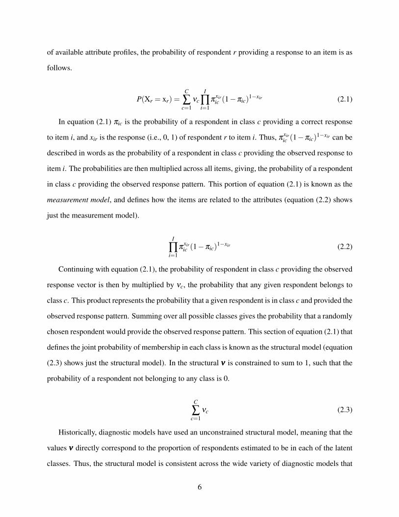
P(Xr = xr) =C
∑c=1
νc
I
∏i=1
πxiric (1−πic)
1−xir (2.1)
In equation (2.1) πic is the probability of a respondent in class c providing a correct response
to item i, and xir is the response (i.e., 0, 1) of respondent r to item i. Thus, πxiric (1−πic)
1−xir can be
described in words as the probability of a respondent in class c providing the observed response to
item i. The probabilities are then multiplied across all items, giving, the probability of a respondent
in class c providing the observed response pattern. This portion of equation (2.1) is known as the
measurement model, and defines how the items are related to the attributes (equation (2.2) shows
just the measurement model).
I
∏i=1
πxiric (1−πic)
1−xir (2.2)
Continuing with equation (2.1), the probability of respondent in class c providing the observed
response vector is then by multiplied by νc, the probability that any given respondent belongs to
class c. This product represents the probability that a given respondent is in class c and provided the
observed response pattern. Summing over all possible classes gives the probability that a randomly
chosen respondent would provide the observed response pattern. This section of equation (2.1) that
defines the joint probability of membership in each class is known as the structural model (equation
(2.3) shows just the structural model). In the structural ννν is constrained to sum to 1, such that the
probability of a respondent not belonging to any class is 0.
C
∑c=1
νc (2.3)
Historically, diagnostic models have used an unconstrained structural model, meaning that the
values ννν directly correspond to the proportion of respondents estimated to be in each of the latent
classes. Thus, the structural model is consistent across the wide variety of diagnostic models that
6
exists. What differs between these models is how the measurement model, or how the items relate
to the attributes. This process begins with the specification of a Q-matrix.
2.1.1 The Q-matrix
The specification of which attributes are measured by each item is defined a priori by the Q-
matrix. The Q-matrix is an n items × a attributes matrix filled with 0s and 1s. A 0 indicates
the item is not measured by the attribute, whereas a 1 indicates that the item is measured by the
attribute (Tatsuoka, 1983). The Q-matrix is developed in consultation with content area experts
to determine the attributes that need to be present in order for the item to be answered correctly
(Bradshaw, 2017). Because the Q-matrix defines how the items relate to the latent attributes, the
correct specification of the Q-matrix is critical to the accuracy of the parameter estimates and
scores. Both Kunina-Habenicht, Rupp, & Wilhelm (2012) and Rupp & Templin (2008a) used
simulation studies to demonstrate the ill-effects of misspecification on classification accuracy and
parameter bias. Given this importance, it is common practice to make changes to the Q-matrix
following the estimation of the DCM (Rupp et al., 2010).
For example de la Torre (2008) proposed a method for empirically validating the Q-matrix fol-
lowing estimation with the deterministic-input, noisy-and-gate model (see section 2.2.1). Using
this method, de la Torre found acceptable Type I and Type II error rates, indicating that the method
was able to adequately identify places where the Q-matrix was both correctly and incorrectly spec-
ified. Similarly, DeCarlo (2011) found that changing the Q-matrix structure could significantly
improve the placement of respondents into latent classes. For example, the initial specification of
the Q-matrix for fraction subtraction data (Tatsuoka, 1990) leads to respondents with no correct
answers mastering the majority of skills. By changing the specification of the Q-matrix, DeCarlo
(2011) was able to correct this, resulting in a more interpretable output. Chen, Liu, Xu, & Ying
(2015) took this approach to the extreme by estimating the entire Q-matrix based only on the
dependencies seen in item responses. Using this method, content experts are removed from the
process of creating the Q-matrix entirely, and it is specified entirely by empirical methods.
7
What the Q-matrix is unable to define is how the attributes interact with each other on a given
item to influence performance. If an item is measured by multiple attributes, does the respondent
have to have mastered all of the attributes in order to have a high probability of answering the
item correctly? Or would mastery of any of the attributes be sufficient? This definition of how the
attributes interact with the items is defined by the measurement model (equation (2.2)). Tradition-
ally, this choice of compensatory versus non-compensatory has been accomplished by choosing
one of a variety of DCMs that have been proposed in the literature.
2.2 Types of DCMs
Traditionally, the type of compensation employed in the measurement model has been defined
through the selection of a specific DCM. The individual types of DCMs each defined the compen-
satory or non-compensatory nature of the attributes and items differently. Thus, the relationships
of attributes and items must be assumed a priori, and then enforced by the selected model. This
relationship can be either non-compensatory or compensatory. Ostensibly, both compensatory and
non-compensatory models could be estimated, compared, and then a final model selected a pos-
teriori; however, usually when selecting one of these models, there is a conceptual reason for the
selection, which may not be compatible with other types of DCMs. Non-compensatory DCMs re-
quire all of the attributes measured by an item to be mastered in order for the item to be answered
correctly. In compensatory DCMs, mastery of some of the attributes measured by an item may be
enough to provide a high probability of success. A high level description of these classes of DCMs
follows.
2.2.1 Noncompensatory DCMs
Non-compensatory DCMs are defined such that all attributes associated with an item must be mas-
tered in order for the respondent to have a high probability of answering the item correctly. In other
words, having an excess of ability on one of the attributes measured by an item cannot make up
8
for the lack of ability on another. This class of DCMs includes the determinisitic-input, noisy-and-
gate (DINA; de la Torre & Douglas, 2004; Haertel, 1989; Junker & Sijtsma, 2001), noisy-input,
deterministic-and gate (NIDA; Henson & Douglas, 2005; Junker & Sijtsma, 2001), and reduced
non-compensatory reparameterized unified (reduced NC-RUM; DiBello, Stout, & Roussos, 1995;
Hartz, 2002) models. In the DINA and NIDA models, there are slipping and guessing parameters
that are held constant across items or attributes respectively. In these models, the slipping parame-
ter represents the probability of incorrectly applying an attribute that has be mastered, whereas the
guessing parameter represents the probability of correctly applying an attribute that hasn’t been
mastered. The reduced NC-RUM is parameterized slightly differently. In this model, the probabil-
ity of providing a correct response when all required attributes have been mastered, with a penalty
factor then applied for each attribute that isn’t mastered. However, in all of these models, the
presence of one of the required attributes is unable to make up for the absence of another.
2.2.2 Compensatory DCMs
In contrast to the non-compensatory DCMs outlined above, compensatory DCMs are structured
such that mastering a subset of the required attributes is sufficient to provide a correct response
to the item. This means that not only a subset attributes that are measured by an item have to
be mastered in order for the respondent to have a high probability of success. DCMs in this
class include the deterministic-input, noisy-or-gate (DINO; Templin & Henson, 2006), noisy-input,
deterministic-or-gate (NIDO; Rupp & Templin, 2008b), compensatory reparameterized unified (C-
RUM; Hartz, 2002) models. The DINO model is parameterized similarly to the DINA and NIDA
models, with slipping and guessing parameters that are held constants across items. However, in
this model, the slipping parameter represents the probability of providing an incorrect response
when at least one of the required attributes has been mastered (rather than when all attributes have
been mastered as in the DINA model). A similar interpretation is made for the guessing parameter.
The NIDO and C-RUM models are parameterized slightly differently. Rather than modeling
parameters on the probability scale, a linear predictor is estimated on the log-odds scale, and then
9
mapped to item scores using the logit link function (see section 2.3.1). In the NIDO model, an
intercept is added to the linear predictor for all attributes measured by the item, and an additional
main effect parameter for each of the mastered attributes. The C-RUM model is similar; however,
rather than an estimating intercept for each attribute, the C-RUM model estimates an intercept for
the entire item, which represents the log-odds of a correct response when none of the measured
attributes are mastered. An additional main effect term is then added for each of the mastered
attributes.
2.3 The log-linear cognitive diagnosis model
The log-linear cognitive diagnosis model (LCDM) is a general framework for diagnostic mod-
els that subsumes most of the existing DCMs, including those discussed in section 2.2 (Henson,
Templin, & Willse, 2008; Rupp et al., 2010). Log-linear models are most commonly used in cate-
gorical data analysis when examining the change in frequency of respondents in a category across
groups (Agresti, 2012). In these models, the frequency of respondents in a category is predicted
by dummy coded grouping variables. Consider an example where a researcher is attempting to
determine if there is a relationship between gender and political party affiliation (for the purposes
of this example this will be limited to democratic or republican). This would result a 2x2 table
similar to Table 2.1.
Table 2.1: Example cross classification
Democratic Republican
Male 400 500Female 600 300
The relationship between gender and party affiliation would be written mathematically as:
ln(Fi j) = λ0 +λGenderi +λ
Partyj +λ
Gender∗Partyi j (2.4)
In equation (2.4) the log frequency of respondents in a cell is given by a linear predictor. The
10
intercept, λ0 represents the frequency for individuals in the reference group for both gender and
party affiliation. The next two terms, λ Genderi and λ
Partyj represent the simple main effects for
gender and party affiliation respectively. Finally, the interaction term, λGender∗Partyi j represents how
related the two factors are. For instance, if gender and party affiliation are completely independent
of one another, the interaction term would be equal to 0.
The LCDM is a log-linear model with categorical latent traits. Consider an item on an achieve-
ment test that measures a single attribute, α1. This would lead to a cross classification table similar
to Table 2.1, but with a latent attribute.
Table 2.2: Example cross classification with latent trait
Master Nonmaster
Correct (X=1) 900 200Incorrect (X=0) 100 600
The mathematical definition of Table 2.2 would be as follows:
ln(Fi j) = λ0 +λα1i +λ
xj +λ
α1∗xi j (2.5)
Table 2.2 and equation (2.5) could both be extended to multiple latent attributes by creating
a three way cross classification table and adding the appropriate main effects and additional in-
teraction terms. Because mastery of the attributes is unobserved, it must be estimated by relating
the observed response to the unobserved attribute. As discussed in section 2.2, the relationship
between observed data and the latent attributes is known as the measurement model.
2.3.1 LCDM measurement model
In order to use a log-linear model to predict probabilities of events occurring (rather than fre-
quencies), a different link function must be used. Equations (2.4) and (2.5) used a log-link, as
frequencies are only bounded on the lower end of the distribution by 0. Probabilities, on the other
hand, are bounded by 0 on the lower and 1 on the upper ends of the distribution. Therefore, a lo-
11
gistic, or logit, link is used. As discussed in section 2.2.2, these types of generalized linear models
involve combining the predictors into what is known as a kernel (or linear predictor in the gener-
alized linear modeling literature; Stroup, 2012), which is an unbounded continuous value that is
mapped to the item responses through a link function. When dealing with dichotomous data, this is
most commonly achieved using the logit link function (Stroup, 2012), defined is in equation (2.6).
ηic = logit(πic) = ln(
πic
1−πic
)(2.6)
Similarly, the inverse of the logit can be expressed as follows.
πic = logit−1(ηic) =exp(ηic)
1+ exp(ηic)(2.7)
The inverse logit in equation (2.7) is more commonly seen in psychometrics, especially in
reference to item response theory (Ayala, 2009).
For the LCDM, the general notation used by Rupp et al. (2010) for parameters in the linear
predictor is λi,l,(a,a′,...). In this notation, the first subscript identifies the item for the parameter,
the second parameter indicates the level of the parameter (i.e., 0 = intercept, 1 = main effect,
2 = two-way interaction, etc.), and the third subscript specifies which attribute(s) are measured
by the parameter. For example, if item 1 on an assessment measured both attributes 1 and 2,
the probability of a correct response would be defined by an intercept, λ0, a simple main effect
for attribute 1, λ1,1,(1), a simple main effect for attribute 2, λ1,1,(2), and the interaction between
attributes 1 and 2 λ1,2,(1,2).
For any number of attributes, A, the kernel for the logit can be defined as follows:
kerneli = λi,0 +A
∑a=1
λi,1,(a)αcaqia + ∑a=1
A
∑a′>1
λi,2,(a,a′)αcaαca′qiaqia′+ ... (2.8)
Equation (2.8) demonstrates that the kernel for item is made up of the intercept, all main effects
for attributes that have both been mastered by individuals in latent class c and are measured by item
i, and all two-way interactions that meet the conditions of all attributes in the interaction have been
12
mastered by latent class c are measured by item i. Equation (2.8) could continue on, adding higher
level interaction terms as more and more attributes are measured by item i, up to the total number
of attributes, A.
Written more succinctly, equation (2.8) can be expressed with matrix notation as:
kerneli = λi,0 +λλλTi h(αααc,qi) (2.9)
For item i, λλλ Ti represents the transpose of the (2A − 1)× 1 vector of item parameters that
contains the main effects and interactions, and h(αααc,qi) is the (2A−1)×1 vector of attribute and
Q-matrix combinations. Thus, written in a more general form, the probability of a respondent in
latent class c providing a correct response to item i can be defined as:
πic = P(Xic = 1 | αααc) =exp(λi,0 +λλλ T
i h(αααc,qi))
1+ exp(λi,0 +λλλ Ti h(αααc,qi))
(2.10)
This expression of a DCM has many advantages over those defined in section 2.2. First, the
LCDM has parameters that are easier to interpret than those seen in the traditional DCMs. For
example, the DINA and NIDA models both contain guessing and slipping parameters, but the
interpretation of them differs due to how parameters are constrained in these models. Additionally,
the slipping parameter (the probability of getting the item wrong despite having mastered all of the
constituent attributes) is less useful than (1−si), or the probability of providing a correct response,
which is usually the value of interest. In contrast, the LCDM parameters are directly analogous
to the parameters of a generalized linear models. Each parameter represents the change in the
log-odds of a correct response.
Additionally, by placing constraints on the parameters of the LCDM, it is possible to estimate
the aforementioned DCMs. For example, the DINA model requires that all attributes be mastered in
order to increase the probability of a correct response. This can be accomplished by constraining
all parameters except the intercept and highest level interaction term of equation (2.8) to be 0
(Henson et al., 2008; Rupp et al., 2010). With these constraints, the log-odds of success are equal
13
to λi,0 when not all attributes have been mastered, and λi,0+λi,2,(a,a′) when all attributes have been
mastered (assuming the item only measures two attributes). The inverse logit (equation (2.7)) of
λi,0 is equal to the guessing parameter gi in the DINA model, and the inverse logit of λi,0+λi,2,(a,a′)
is equal to (1− si).
Similarly, the DINO model can also be replicated through constraints on the LCDM model.
In the DINO model, mastering one attribute is just as good as mastering a different or multiple
attributes that are measured by the item. Thus, the first constraint is that the main effects must
be equal. If an item measures two attributes, the increase in the log-odds of providing a correct
response is equal, regardless of which of the two is mastered. The second constraint is that the
interaction term is equal to the negative of the main effect parameter. This means that three param-
eters (two main effects and an interaction) all have the same absolute value, but the main effects
are positive and the interaction is negative. This has the effect of the interaction cancelling out the
additional increase in log-odds of a correct response for mastering additional attributes. Thus, the
kernel for LCDM parameterization of the DINO model can be written as:
kerneli = λi,0 +λiα1 +λiα2−λiα1α2
= λi,0 +λi(α1 +α2−α1α2)(2.11)
When neither of the attributes measured by the item have been mastered, α1 and α2 are 0, and
equation (2.11) simplifies to λi,0, which is equivalent to the inverse logit of gi in the DINO model.
If only attribute 1 has been mastered, the α2 will be equal to 0, and equation (2.11) simplifies to
λi,0 +λi, which is equivalent to (1− si) in the DINO model. Finally, if both attributes have been
mastered, then equation (2.11) becomes λi,0 +λi(1+1−1×1) = λi,0 +λi, which is identical the
result when only one attribute was mastered.
Because the LCDM is able to encompass this variety of DCMs, the choice of compensatory
versus non-compensatory DCM becomes irrelevant. Instead, the saturated LCDM can be esti-
mated, and if the items truly follow the DINA, DINO, or other lower-level DCM, the estimated
14
parameters will reflect this. Further the LCDM provides a framework for testing the assumptions
of these other DCMs. For example, two models could be fit to the same data: one fully saturated
LCDM, the other with constraints on the item parameters. A likelihood ratio test can then be
performed to determine if the reduced model fits as well as the saturated model.
2.4 Structural models
To this point, the discussion has focused on the measurement model of DCMs. Recall from equa-
tion (2.1), reprinted here, that this is only one piece of the diagnostic model.
P(Xr = xr) =C
∑c=1
νc
I
∏i=1
πxiric (1−πic)
1−xir (2.12)
The measurement model, which relates the attributes to the observed item responses, is con-
cerned with estimated πic. The structural model is focused on νc. In DCMs, νc represents the
base rate probability of each latent class (Rupp et al., 2010). The base probabilities allow for the
calculation of mastery rates for each attribute marginally, as well as the correlations between the
attributes. In an assessment with A attributes there are 2A latent classes. Because all elements of
ν must sum to 0, there are 2A−1 parameters to estimate, as the final element can be calculated by
taking 1 minus the sum of the other elements.
Estimating each of these probabilities directly is referred to as the “unstructured” or “uncon-
strained” structural model (Rupp et al., 2010). By estimating the probabilities directly, it is possible
to observe if there are any classes that have few respondents, possibly indicating the presence of
an attribute hierarchy as described by (Templin & Bradshaw, 2014a). However, this type of uncon-
strained model can cause problems in high dimensional attribute spaces. Because the number of
structural parameters to be estimated is 2A−1, the number of parameters increases exponentially
with each added attribute. For example, a five attribute assessment requires 25− 1 = 31 parame-
ters, whereas a 10 attribute assessment would require 210−1 = 1,023 parameters. Thus, it is often
desirable to reduce the number of parameters that need to be estimated.
15
Two such approaches for reducing the structural model are the unstructured tetrachoric model
(Hartz, 2002) and structured tetrachoric model (de la Torre & Douglas, 2004). These approaches
work well in many instances (e.g., if the primary interest is the relationships between the attributes),
however, they can be rather restrictive in what can be estimated. For example, suppose that and
unstructured tetrachoric model is utilized, and it is determined that the structural model has been
reduced too much. With this method, it is not a straightforward proposition as to how to add
parameters back in without going all the way back to the unconstrained model. Additionally,
suppose that a researcher is interested in both the potential hierarchical structure of attributes and
the attributes’ associations. How should the researcher reduce the model, and achieve both of these
desired outcomes? Rupp et al. (2010) suggest a “top-down approach” using log-linear models,
which is described in the following section (section 2.4.1).
2.4.1 Log-linear structural models
The log-linear approach to structural models was proposed by (Henson & Templin, 2005), and is
very similar to the log-linear model that was used to define the measurement model of the LCDM
in section 2.3.1. Specifically, the kernel for latent class c can be defined as follows:
kernelc =A
∑a=1
γ1,(a)αca +A−1
∑a=1
A
∑a′=a+1
γ2,(a,a′)αcaαca′+ ...+ γA,(a,a′,...)
A
∏a=1
αca (2.13)
The parameters included for latent class c are a main effect for each attribute that has been
mastered by individuals in the class, as well interactions between the mastered attributes (two-way
up to A-way, where A is the total number of attributes assessed). For an assessment measuring two
attributes, the structural model would be defined as outlined in Table 2.3.
The fully saturated log-linear structural model is equivalent to the unconstrained structural
model. However, this parameterization has many benefits over the tetrachoric methods. First,
using this method allows for a hypothesis test on each of the estimated parameters. Thus, non-
significant parameters can be removed from the model, allowing for model reduction to occur
16
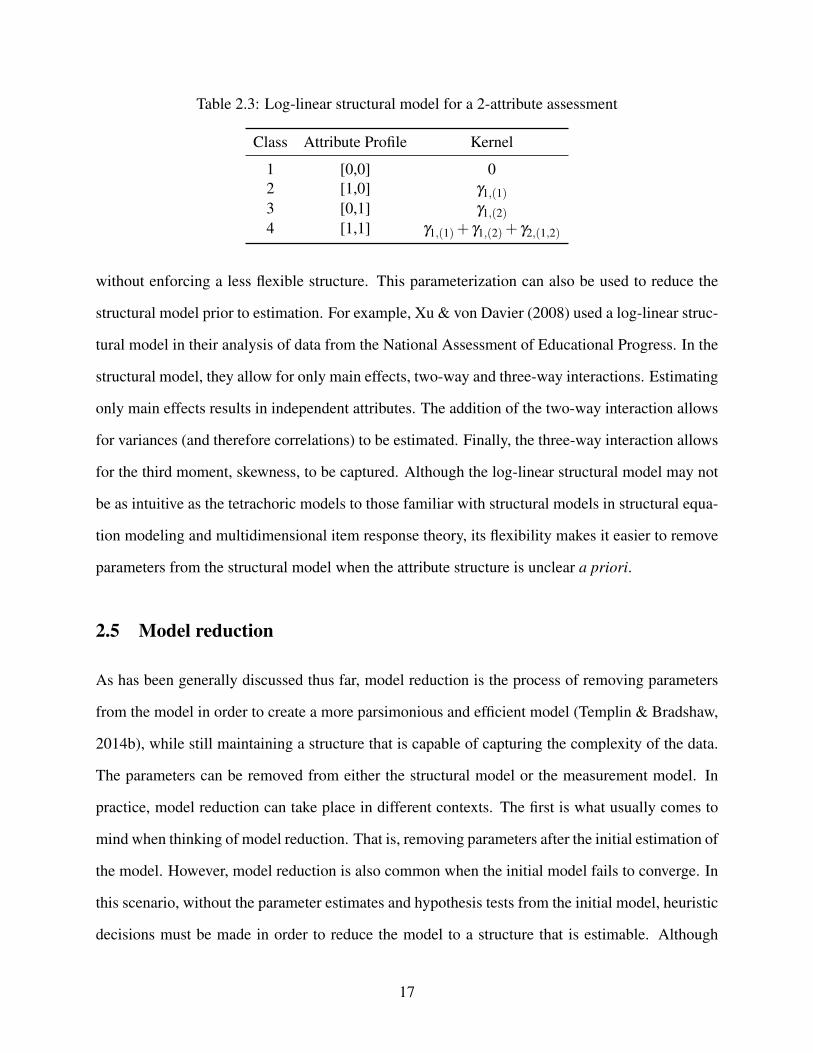
Table 2.3: Log-linear structural model for a 2-attribute assessment
Class Attribute Profile Kernel
1 [0,0] 02 [1,0] γ1,(1)3 [0,1] γ1,(2)4 [1,1] γ1,(1)+ γ1,(2)+ γ2,(1,2)
without enforcing a less flexible structure. This parameterization can also be used to reduce the
structural model prior to estimation. For example, Xu & von Davier (2008) used a log-linear struc-
tural model in their analysis of data from the National Assessment of Educational Progress. In the
structural model, they allow for only main effects, two-way and three-way interactions. Estimating
only main effects results in independent attributes. The addition of the two-way interaction allows
for variances (and therefore correlations) to be estimated. Finally, the three-way interaction allows
for the third moment, skewness, to be captured. Although the log-linear structural model may not
be as intuitive as the tetrachoric models to those familiar with structural models in structural equa-
tion modeling and multidimensional item response theory, its flexibility makes it easier to remove
parameters from the structural model when the attribute structure is unclear a priori.
2.5 Model reduction
As has been generally discussed thus far, model reduction is the process of removing parameters
from the model in order to create a more parsimonious and efficient model (Templin & Bradshaw,
2014b), while still maintaining a structure that is capable of capturing the complexity of the data.
The parameters can be removed from either the structural model or the measurement model. In
practice, model reduction can take place in different contexts. The first is what usually comes to
mind when thinking of model reduction. That is, removing parameters after the initial estimation of
the model. However, model reduction is also common when the initial model fails to converge. In
this scenario, without the parameter estimates and hypothesis tests from the initial model, heuristic
decisions must be made in order to reduce the model to a structure that is estimable. Although
17
different, understanding these processes is critical to the interpretation of the results. Before ex-
amining prior research on this using DCMs, the related literature from other latent variable models
such as structural equation modeling and item response theory will be examined.
2.5.1 Model reduction in structural equation modeling
As in DCMs, in structural equation modeling, the measurement model relates the observed vari-
ables to the latent traits and the structural model defines the relationships between the latent traits.
As such, both parts of the structural equation model can be reduced. In practice, this is a multi-
stage process. Both Kline (2002) and Ullman (2012) suggest first fitting each measurement model
separately. In other words, for each latent variable, fit a unidimensional model first. Then, add
or remove parameters as necessary in order to ensure model fit. Once all of the unidimensional
models have been assessed for model fit, they can be estimated simultaneously in the structural
equation model, and the structural model can be reparameterized as needed to ensure the fit of the
whole model.
Thus, the structural equation modeling world seems to follow a measurement model first, then
structural model approach to model reduction. In an examination of the relationships between
mental toughness, motivation, and emotion in sports, Perry, Nicholls, Clough, & Crust (2015) ex-
amined the factors from each questionnaire separately before combining them into the full model.
They found that the full model had significantly better fit when the measurement models were ad-
justed prior to the estimation of the full model. Similarly, Burkholder & Harlow (2003) followed
this procedure to reduce their model investigating HIV behavior risk. In this model, there was
no reduction of the measurement model as each factor was just-identified. Thus, there was only
reduction at the structural level, where all non-significant regression coefficients were removed.
However, it should be noted that model modifications are not limited to the removal of pa-
rameters in structural equation models. It is also common to use modification indices to locate
places in the model where there is misfit and add parameters to improve the overall fit (Brown,
2006; Kaplan, 2009). These parameters could include additional regression paths, covariances be-
18
tween latent factors, or residual covariances. Thus, when structural equation models are modified
following the initial estimation it is common practice to not only reduce the model by removing
non-significant parameters, but also add additional parameters in order to ensure model fit.
2.5.2 Model reduction in item response theory
Unlike structural equation modeling, model reduction is relatively uncommon in item response
theory. There are a few possible reasons for this. First, the majority of operationally used item
response theory models are unidimensional, with multidimensional item response theory models
having yet to see wide spread operational use (see Fukuhara & Kamata, 2011; Reckase, 1997;
Sinharay, 2010; Thissen & Steinberg, 1986). In unidimensional models, there are no relationships
between latent variables to estimate, as there is only one. Thus, only the measurement model is
of consequence. In unidimensional item response theory models, this comes down to the selection
of the number of parameters to be included (i.e., 1-parameter logistic model, 2-parameter logistic
model, or 3-parameter model). Thus, after choosing an initial model, the options are to either
reduce the model by removing items that don’t fit, or change models to add additional parameters.
In contrast, multidimensional item response theory models do offer opportunities for model re-
duction. In multidimensional models, the covariance structure of the latent factors can be reduced,
as well as respecifying the latent traits that are measured by each item. However, although there are
a few examples of various specifications being tested (see Kingston & McKinley, 1988; McKinley
& Kingston, 1988), this is typically not done in practice. Indeed, there is no mention at all of
modifying the structure of the multidimensional model following estimation in the most widely
cited textbook on multidimensional item response theory models (see Reckase, 2009). Instead, a
saturated covariance matrix is estimated for the latent traits, and decisions about the measurement
model parameters are confined to removing items that don’t fit the model.
19
2.5.3 Model reduction in DCMs
In diagnostic models, the model reduction process is more similar to structural equation modeling
than item response theory, in that it is a common practice to reduce the model by removing non-
significant parameters after the estimation of the initial model. For example, Jurich & Bradshaw
(2013) used the LCDM with a log-linear structural model to scale the Socialcultural Dimension
Assessment version 6 (Halonen, Harris, Pastor, Abrahamson, & Huffman, 2005). In the estimation
of the LCDM, four separate structural models were defined a priori: the fully saturated log-linear
model, reduced model where three- and four-way interactions were removed (constrained to be 0),
and a model with only main effects and two-way interactions that were constrained to be equal.
Initially, Jurich & Bradshaw (2013) estimated the model with a fully saturated measurement and
structural model. Following this initial estimation they removed non-significant parameters from
the measurement model, before using the reduced measurement model to evaluate the structural
models.
A similar approach was used by Bradshaw, Izsák, Templin, & Jacobson (2014) in their analysis
of the Diagnosing Teachers’ Multiplicative Reasoning assessment. In this analysis, a fully satu-
rated LCDM and log-linear structural model were used in the initial estimation. However, when
three- and four-way interaction terms were specified in the structural model, the model was not able
to converge. Thus, they settled on a reduced structural model with only main effects and two-way
interactions included. Using the reduced structural model, Bradshaw et al. proceeded to remove
non-significant terms from the measurement model. This same procedure was followed by de la
Torre, Ark, & Rossi (2015) in their analysis of the Dutch version of the Millon Clinical Multiaxial
Inventory-III (T. Millon, Millon, Davis, & Grossman, 2009). Using a saturated structural model,
the measurement model was reduced by removing non-significant terms from each item. However,
no further model reduction was done to the structural model.
As can be seen from these studies, there is an inconsistency as to the order in which model
reduction should occur in DCMs. Bradshaw et al. (2014) reduced the structural model first out
of necessity due to convergence, whereas Jurich & Bradshaw (2013) elected to reduce the mea-
20
surement model first. However, this has not, to this point, been an investigation as to which of the
processes should be preferred.
One option would be to follow the direction of the structural equation modeling literature and
always reduce the measurement model first. This is potentially problematic for a few reasons.
First, structural equation models assume that the data is normally distributed, whereas diagnostic
models assume dichotomous items. It is possible to have non-dichotomous data (e.g., Skrondal &
Rabe-Hesketh, 2004), but that is beyond the scope of this study. Additionally the latent variables
in structural equation models are generally continuous, whereas DCMs use categorical latent vari-
ables. Because the observed data and latent variable space both follow different distributions, it’s
possible that the best practices may differ between the two models.
Additionally, there is the added complexity of precisely how the measurement model is esti-
mated in structural equation models. Recall from section 2.5.1 that the recommended practice to
estimate each latent variable’s own measurement model first in order to ensure fit (Kline, 2002).
However the measurement model for DCMs require multiple attributes in order to estimate the
interaction effects (see equation (2.8)). Thus, the measurement models could only be estimated
separately when there was a simple specification of the Q-matrix where each item measured only
one attribute. Therefore, the approach taken by the structural equation modeling community is
unlikely to be feasible for most DCM assessments.
2.6 The current study
Despite the uncertainty in the process of model reduction, this is a crucial aspect of DCM estima-
tion. Rojas, de la Torre, & Olea (2012) showed that estimating high level interaction terms when
unnecessary can decrease the classification accuracy compared to a reduced model. However, Ro-
jas et al. (2012) only examined reduction of the measurement model. Therefore, the present study
seeks to examine reduction of both the measurement and structural models to answer the following
research questions:
21
1. Does choosing different a model reduction process impact the output of the model?
2. What are the benefits of reducing the measurement and/or structural model(s)?
3. Are there advantages or disadvantages to the order of reduction (i.e., measurement or struc-
tural reduction first)?
This is accomplished through two studies. The first is a pilot study to further demonstrate the
importance of the order of model reduction. Specifically the Diagnosing Teachers’ Multiplicative
Reasoning assessment data (as described in Bradshaw et al., 2014) is reduced in different orders
to compare the values of the resulting parameter estimates. Second, given the results of the pilot
study, and Monte Carlo simulation study is conducted to examine the effects of model reduction
and the order of reduction under a variety of data generation and dimensionality conditions.
22
Chapter 3
Pilot Study
In order to better assess the impact of the order of model reduction, a pilot study was conducted
on the Diagnosing Teachers’ Multiplicative Reasoning (DTMR) assessment data, as described in
Bradshaw et al. (2014). In this study, the DTMR data set was analyzed using a variety of model
reduction processes to determine if the selected process has an impact on the resulting model
parameters. Thus, the pilot study was designed to answer the first research question defined in
section 2.6. This is an important first step as without evidence that the model reduction process
has an impact on the results, there would be little motivation for a more thorough analysis via
simulation.
3.1 Method
3.1.1 DTMR data
The DTMR assessment consists of 28 dichotomously scored items that together measure 4 at-
tributes related to educators’ understanding of multiplicative reasoning (Bradshaw et al., 2014):
1. Referent Units (RU): recognizing which whole the fraction refers to,
2. Partitioning and Iterating (PI): splitting a whole into equal pieces repeatedly to achieve larger
fractions,
3. Appropriateness (APP): determining the correct mathematical operation from a problem
statement, and
4. Multiplicative Comparison (MC): evaluating the ratio of one value to another.
23
Of the 28 items, Referent Units is measured by 16, Partitioning and Iterating by 10, Appro-
priateness by 6, and Multiplicative Comparison by 10. This totals adds to more than 28 because
several items measure more than one attribute. Specifically, there are 14 items measuring only
1 attribute and 14 that measure 2 attributes. The complete saturated Q-matrix for the DTMR as-
sessment can be see in Table 3.1. For example, item 1 measures only the Referent Units attribute,
whereas item 5 measures both the Referent Units and Multiplicative Comparison attributes.
Table 3.1: DTMR Q-matrix
Item Item Name RU PI APP MC
1 1 1 0 0 02 2 0 0 1 03 3 0 1 0 04 4 1 0 0 05 5 1 0 0 1
6 6 0 1 0 07 7 1 0 0 08 8a 0 0 1 19 8b 0 0 1 0
10 8c 0 0 1 0
11 8d 0 0 1 012 9 1 0 0 013 10a 1 0 0 114 10b 1 0 0 115 10c 1 0 0 1
16 11 1 0 0 117 12 1 0 0 018 13 0 1 0 119 14 1 1 0 020 15a 0 1 0 1
21 15b 0 1 0 122 15c 0 1 0 123 16 1 0 0 024 17 1 1 0 025 18 1 1 0 0
26 19 0 0 1 027 21 1 0 0 028 22 1 1 0 0
24
In total 990 math teachers took the assessment. Bradshaw et al. (2014) reported that sample
demographics were consistent with a representative national sample. For a complete description
of the sample characteristics and data collection process, see the original description of the DTMR
in Bradshaw et al. (2014).
3.1.2 Model estimation
In order to assess the impact of various model reduction processes, the LCDM was estimated for
the DTRM using five different reduction methods:
1. Simultaneous reduction: after estimating the fully saturated model, all non-significant pa-
rameters from both the measurement and the structural models are removed and the model
is re-estimated,
2. Measurement reduction: after estimating the fully saturated model, all non-significant pa-
rameters from the measurement model only are removed and the model is re-estimated,
3. Structural reduction: after estimating the fully saturated model, all non-significant parame-
ters from the structural model only are removed and the model is re-estimated,
4. Measurement-Structural reduction: after estimating the measurement reduction model, all
non-significant parameters from the structural model only are removed and the model is
re-estimated, and
5. Structural-Measurement reduction: after estimating the structural reduction model, all non-
significant parameters from the measurement model only are removed and the model is re-
estimated.
The different ordering processes for model reduction, and their relationships to each other,
are represented visually in Figure 3.1. The significance of each parameter was determined by
the p-value derived from the Wald test provided by Mplus. This test provides a p-value for the
null hypothesis that the parameter is equal to zero. Parameters with a p-value greater than 0.05
were determined to be non-significant, and therefore removed at the corresponding stage of model
25
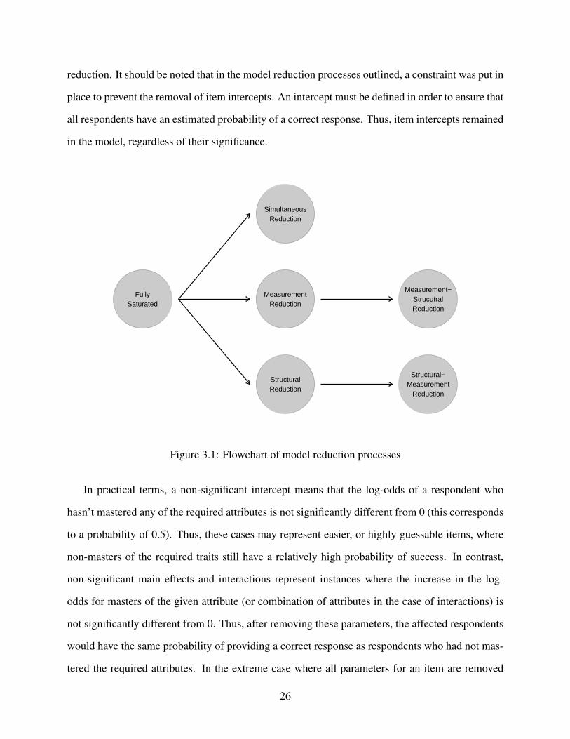
reduction. It should be noted that in the model reduction processes outlined, a constraint was put in
place to prevent the removal of item intercepts. An intercept must be defined in order to ensure that
all respondents have an estimated probability of a correct response. Thus, item intercepts remained
in the model, regardless of their significance.
FullySaturated
SimultaneousReduction
MeasurementReduction
StructuralReduction
Measurement−StrucutralReduction
Structural−Measurement
Reduction
Figure 3.1: Flowchart of model reduction processes
In practical terms, a non-significant intercept means that the log-odds of a respondent who
hasn’t mastered any of the required attributes is not significantly different from 0 (this corresponds
to a probability of 0.5). Thus, these cases may represent easier, or highly guessable items, where
non-masters of the required traits still have a relatively high probability of success. In contrast,
non-significant main effects and interactions represent instances where the increase in the log-
odds for masters of the given attribute (or combination of attributes in the case of interactions) is
not significantly different from 0. Thus, after removing these parameters, the affected respondents
would have the same probability of providing a correct response as respondents who had not mas-
tered the required attributes. In the extreme case where all parameters for an item are removed
26
except for the intercept, all respondents would have the same probability of success, regardless of
their profile of attribute mastery.
All analyses for the pilot study were conducted in Mplus version 7.4 (L. K. Muthén & Muthén,
1998) via the MplusAutomation package (Hallquist & Wiley, 2018) in R version 3.4.3 (R Core
Team, 2017). Mplus code for the estimation of the LCDM was generated in R using custom scripts
based on the work of Rupp & Wilhelm (2012) and Templin & Hoffman (2013).
3.2 Results
The final estimate and associated standard error for each parameter from each of the model reduc-
tion processes are presented in their own tables in order to easily compare across model reduction
processes. Table 3.2, Table 3.3, Table 3.4, Table 3.5, Table 3.6, Table 3.7, Table 3.8, Table 3.9,
and Table 3.10 show the results of the measurement model parameters, and Table 3.11 shows the
results of the structural model parameters.
3.2.1 Measurement model results
Although it is tempting to compare the point estimates and standard errors for the parameters
across model reduction techniques, this is ill-advised. Because the main effects and interactions
are conditional on other parameters in the model, the exclusion of parameters will change the
interpretation of the other parameters. Thus, changes in point estimates and standard errors may
be expected. Thus, these results are most useful for comparing which parameters are ultimately
retained in the model. In general we can see that the choice of the model reduction method can
have a profound impact on which parameters are ultimately retained in the model. The exception
to this is the item intercepts (Table 3.2). Because model reduction was constrained to never remove
item intercepts, all intercepts are estimated, no matter which reduction technique was used. This is
not the case for main effects. For example, when examining the main effects for attribute 1 (Table
3.3), the main effect for item 13 was only retained when either the structural model only was
27
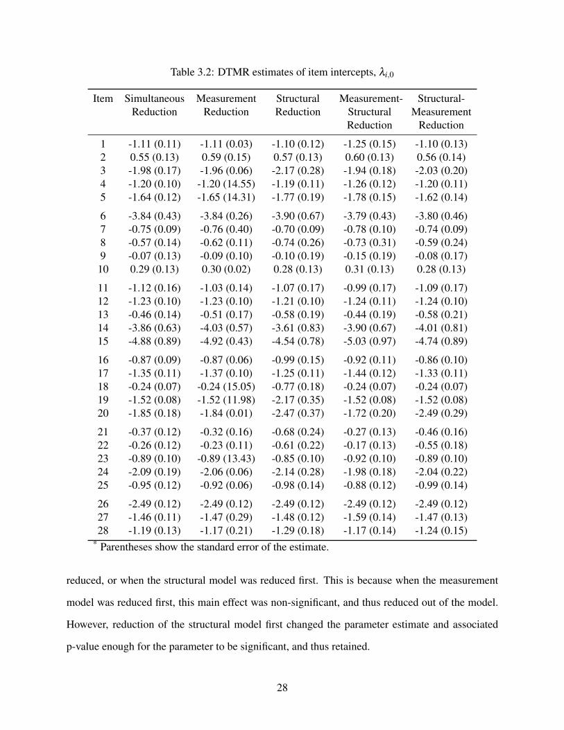
Table 3.2: DTMR estimates of item intercepts, λi,0
Item SimultaneousReduction
MeasurementReduction
StructuralReduction
Measurement-StructuralReduction
Structural-Measurement
Reduction
1 -1.11 (0.11) -1.11 (0.03) -1.10 (0.12) -1.25 (0.15) -1.10 (0.13)2 0.55 (0.13) 0.59 (0.15) 0.57 (0.13) 0.60 (0.13) 0.56 (0.14)3 -1.98 (0.17) -1.96 (0.06) -2.17 (0.28) -1.94 (0.18) -2.03 (0.20)4 -1.20 (0.10) -1.20 (14.55) -1.19 (0.11) -1.26 (0.12) -1.20 (0.11)5 -1.64 (0.12) -1.65 (14.31) -1.77 (0.19) -1.78 (0.15) -1.62 (0.14)
6 -3.84 (0.43) -3.84 (0.26) -3.90 (0.67) -3.79 (0.43) -3.80 (0.46)7 -0.75 (0.09) -0.76 (0.40) -0.70 (0.09) -0.78 (0.10) -0.74 (0.09)8 -0.57 (0.14) -0.62 (0.11) -0.74 (0.26) -0.73 (0.31) -0.59 (0.24)9 -0.07 (0.13) -0.09 (0.10) -0.10 (0.19) -0.15 (0.19) -0.08 (0.17)
10 0.29 (0.13) 0.30 (0.02) 0.28 (0.13) 0.31 (0.13) 0.28 (0.13)
11 -1.12 (0.16) -1.03 (0.14) -1.07 (0.17) -0.99 (0.17) -1.09 (0.17)12 -1.23 (0.10) -1.23 (0.10) -1.21 (0.10) -1.24 (0.11) -1.24 (0.10)13 -0.46 (0.14) -0.51 (0.17) -0.58 (0.19) -0.44 (0.19) -0.58 (0.21)14 -3.86 (0.63) -4.03 (0.57) -3.61 (0.83) -3.90 (0.67) -4.01 (0.81)15 -4.88 (0.89) -4.92 (0.43) -4.54 (0.78) -5.03 (0.97) -4.74 (0.89)
16 -0.87 (0.09) -0.87 (0.06) -0.99 (0.15) -0.92 (0.11) -0.86 (0.10)17 -1.35 (0.11) -1.37 (0.10) -1.25 (0.11) -1.44 (0.12) -1.33 (0.11)18 -0.24 (0.07) -0.24 (15.05) -0.77 (0.18) -0.24 (0.07) -0.24 (0.07)19 -1.52 (0.08) -1.52 (11.98) -2.17 (0.35) -1.52 (0.08) -1.52 (0.08)20 -1.85 (0.18) -1.84 (0.01) -2.47 (0.37) -1.72 (0.20) -2.49 (0.29)
21 -0.37 (0.12) -0.32 (0.16) -0.68 (0.24) -0.27 (0.13) -0.46 (0.16)22 -0.26 (0.12) -0.23 (0.11) -0.61 (0.22) -0.17 (0.13) -0.55 (0.18)23 -0.89 (0.10) -0.89 (13.43) -0.85 (0.10) -0.92 (0.10) -0.89 (0.10)24 -2.09 (0.19) -2.06 (0.06) -2.14 (0.28) -1.98 (0.18) -2.04 (0.22)25 -0.95 (0.12) -0.92 (0.06) -0.98 (0.14) -0.88 (0.12) -0.99 (0.14)
26 -2.49 (0.12) -2.49 (0.12) -2.49 (0.12) -2.49 (0.12) -2.49 (0.12)27 -1.46 (0.11) -1.47 (0.29) -1.48 (0.12) -1.59 (0.14) -1.47 (0.13)28 -1.19 (0.13) -1.17 (0.21) -1.29 (0.18) -1.17 (0.14) -1.24 (0.15)
* Parentheses show the standard error of the estimate.
reduced, or when the structural model was reduced first. This is because when the measurement
model was reduced first, this main effect was non-significant, and thus reduced out of the model.
However, reduction of the structural model first changed the parameter estimate and associated
p-value enough for the parameter to be significant, and thus retained.
28
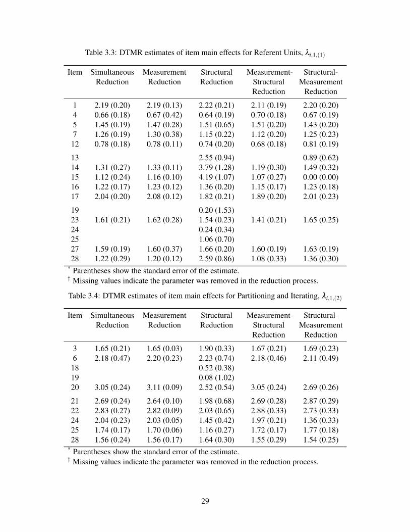
Table 3.3: DTMR estimates of item main effects for Referent Units, λi,1,(1)
Item SimultaneousReduction
MeasurementReduction
StructuralReduction
Measurement-StructuralReduction
Structural-Measurement
Reduction
1 2.19 (0.20) 2.19 (0.13) 2.22 (0.21) 2.11 (0.19) 2.20 (0.20)4 0.66 (0.18) 0.67 (0.42) 0.64 (0.19) 0.70 (0.18) 0.67 (0.19)5 1.45 (0.19) 1.47 (0.28) 1.51 (0.65) 1.51 (0.20) 1.43 (0.20)7 1.26 (0.19) 1.30 (0.38) 1.15 (0.22) 1.12 (0.20) 1.25 (0.23)
12 0.78 (0.18) 0.78 (0.11) 0.74 (0.20) 0.68 (0.18) 0.81 (0.19)
13 2.55 (0.94) 0.89 (0.62)14 1.31 (0.27) 1.33 (0.11) 3.79 (1.28) 1.19 (0.30) 1.49 (0.32)15 1.12 (0.24) 1.16 (0.10) 4.19 (1.07) 1.07 (0.27) 0.00 (0.00)16 1.22 (0.17) 1.23 (0.12) 1.36 (0.20) 1.15 (0.17) 1.23 (0.18)17 2.04 (0.20) 2.08 (0.12) 1.82 (0.21) 1.89 (0.20) 2.01 (0.23)
19 0.20 (1.53)23 1.61 (0.21) 1.62 (0.28) 1.54 (0.23) 1.41 (0.21) 1.65 (0.25)24 0.24 (0.34)25 1.06 (0.70)27 1.59 (0.19) 1.60 (0.37) 1.66 (0.20) 1.60 (0.19) 1.63 (0.19)28 1.22 (0.29) 1.20 (0.12) 2.59 (0.86) 1.08 (0.33) 1.36 (0.30)
* Parentheses show the standard error of the estimate.† Missing values indicate the parameter was removed in the reduction process.
Table 3.4: DTMR estimates of item main effects for Partitioning and Iterating, λi,1,(2)
Item SimultaneousReduction
MeasurementReduction
StructuralReduction
Measurement-StructuralReduction
Structural-Measurement
Reduction
3 1.65 (0.21) 1.65 (0.03) 1.90 (0.33) 1.67 (0.21) 1.69 (0.23)6 2.18 (0.47) 2.20 (0.23) 2.23 (0.74) 2.18 (0.46) 2.11 (0.49)
18 0.52 (0.38)19 0.08 (1.02)20 3.05 (0.24) 3.11 (0.09) 2.52 (0.54) 3.05 (0.24) 2.69 (0.26)
21 2.69 (0.24) 2.64 (0.10) 1.98 (0.68) 2.69 (0.28) 2.87 (0.29)22 2.83 (0.27) 2.82 (0.09) 2.03 (0.65) 2.88 (0.33) 2.73 (0.33)24 2.04 (0.23) 2.03 (0.05) 1.45 (0.42) 1.97 (0.21) 1.36 (0.33)25 1.74 (0.17) 1.70 (0.06) 1.16 (0.27) 1.72 (0.17) 1.77 (0.18)28 1.56 (0.24) 1.56 (0.17) 1.64 (0.30) 1.55 (0.29) 1.54 (0.25)
* Parentheses show the standard error of the estimate.† Missing values indicate the parameter was removed in the reduction process.
29
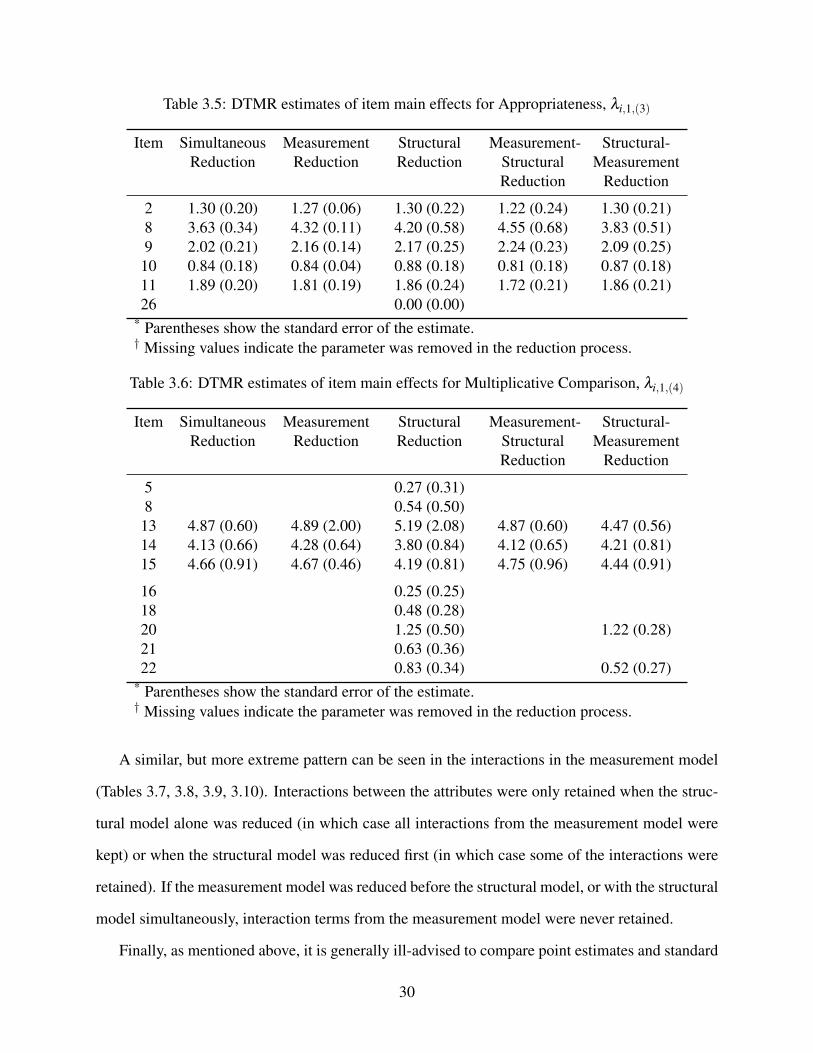
Table 3.5: DTMR estimates of item main effects for Appropriateness, λi,1,(3)
Item SimultaneousReduction
MeasurementReduction
StructuralReduction
Measurement-StructuralReduction
Structural-Measurement
Reduction
2 1.30 (0.20) 1.27 (0.06) 1.30 (0.22) 1.22 (0.24) 1.30 (0.21)8 3.63 (0.34) 4.32 (0.11) 4.20 (0.58) 4.55 (0.68) 3.83 (0.51)9 2.02 (0.21) 2.16 (0.14) 2.17 (0.25) 2.24 (0.23) 2.09 (0.25)
10 0.84 (0.18) 0.84 (0.04) 0.88 (0.18) 0.81 (0.18) 0.87 (0.18)11 1.89 (0.20) 1.81 (0.19) 1.86 (0.24) 1.72 (0.21) 1.86 (0.21)26 0.00 (0.00)
* Parentheses show the standard error of the estimate.† Missing values indicate the parameter was removed in the reduction process.
Table 3.6: DTMR estimates of item main effects for Multiplicative Comparison, λi,1,(4)
Item SimultaneousReduction
MeasurementReduction
StructuralReduction
Measurement-StructuralReduction
Structural-Measurement
Reduction
5 0.27 (0.31)8 0.54 (0.50)
13 4.87 (0.60) 4.89 (2.00) 5.19 (2.08) 4.87 (0.60) 4.47 (0.56)14 4.13 (0.66) 4.28 (0.64) 3.80 (0.84) 4.12 (0.65) 4.21 (0.81)15 4.66 (0.91) 4.67 (0.46) 4.19 (0.81) 4.75 (0.96) 4.44 (0.91)
16 0.25 (0.25)18 0.48 (0.28)20 1.25 (0.50) 1.22 (0.28)21 0.63 (0.36)22 0.83 (0.34) 0.52 (0.27)
* Parentheses show the standard error of the estimate.† Missing values indicate the parameter was removed in the reduction process.
A similar, but more extreme pattern can be seen in the interactions in the measurement model
(Tables 3.7, 3.8, 3.9, 3.10). Interactions between the attributes were only retained when the struc-
tural model alone was reduced (in which case all interactions from the measurement model were
kept) or when the structural model was reduced first (in which case some of the interactions were
retained). If the measurement model was reduced before the structural model, or with the structural
model simultaneously, interaction terms from the measurement model were never retained.
Finally, as mentioned above, it is generally ill-advised to compare point estimates and standard
30
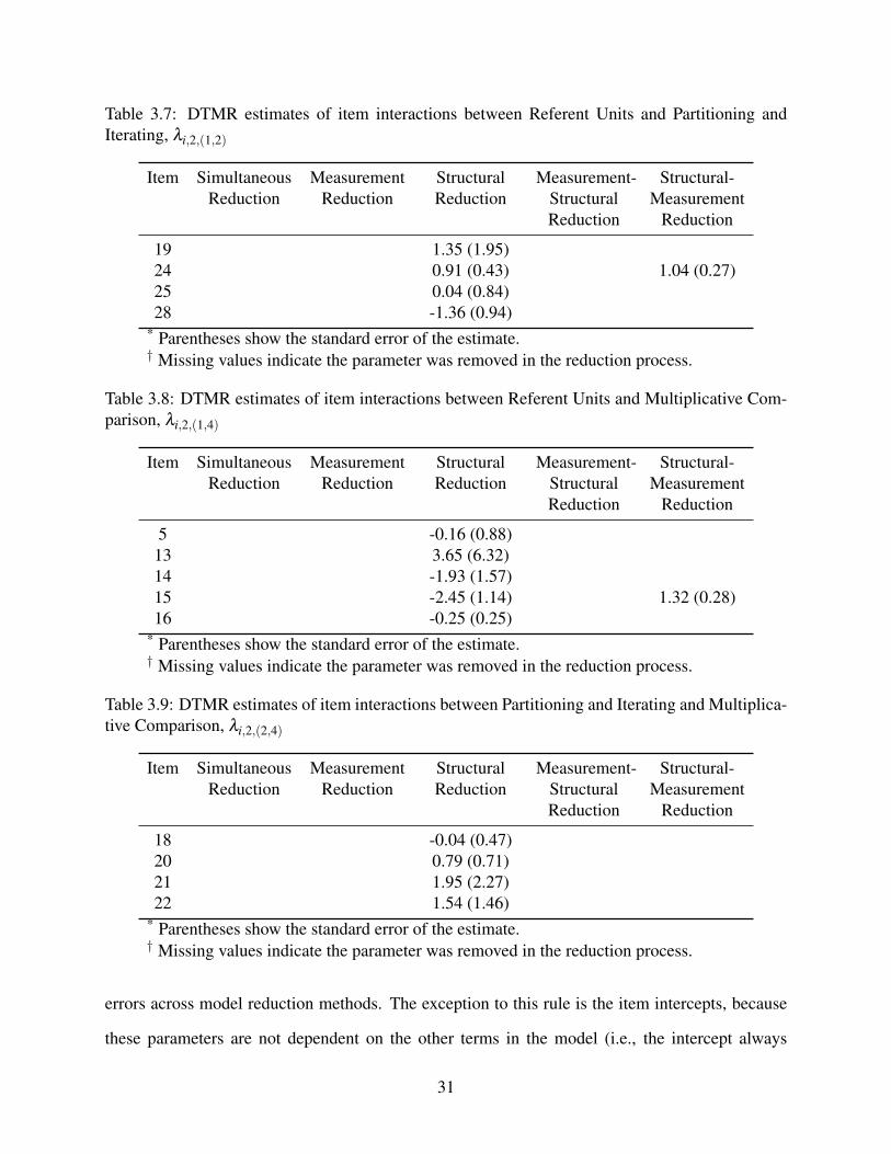
Table 3.7: DTMR estimates of item interactions between Referent Units and Partitioning andIterating, λi,2,(1,2)
Item SimultaneousReduction
MeasurementReduction
StructuralReduction
Measurement-StructuralReduction
Structural-Measurement
Reduction
19 1.35 (1.95)24 0.91 (0.43) 1.04 (0.27)25 0.04 (0.84)28 -1.36 (0.94)
* Parentheses show the standard error of the estimate.† Missing values indicate the parameter was removed in the reduction process.
Table 3.8: DTMR estimates of item interactions between Referent Units and Multiplicative Com-parison, λi,2,(1,4)
Item SimultaneousReduction
MeasurementReduction
StructuralReduction
Measurement-StructuralReduction
Structural-Measurement
Reduction
5 -0.16 (0.88)13 3.65 (6.32)14 -1.93 (1.57)15 -2.45 (1.14) 1.32 (0.28)16 -0.25 (0.25)
* Parentheses show the standard error of the estimate.† Missing values indicate the parameter was removed in the reduction process.
Table 3.9: DTMR estimates of item interactions between Partitioning and Iterating and Multiplica-tive Comparison, λi,2,(2,4)
Item SimultaneousReduction
MeasurementReduction
StructuralReduction
Measurement-StructuralReduction
Structural-Measurement
Reduction
18 -0.04 (0.47)20 0.79 (0.71)21 1.95 (2.27)22 1.54 (1.46)
* Parentheses show the standard error of the estimate.† Missing values indicate the parameter was removed in the reduction process.
errors across model reduction methods. The exception to this rule is the item intercepts, because
these parameters are not dependent on the other terms in the model (i.e., the intercept always
31
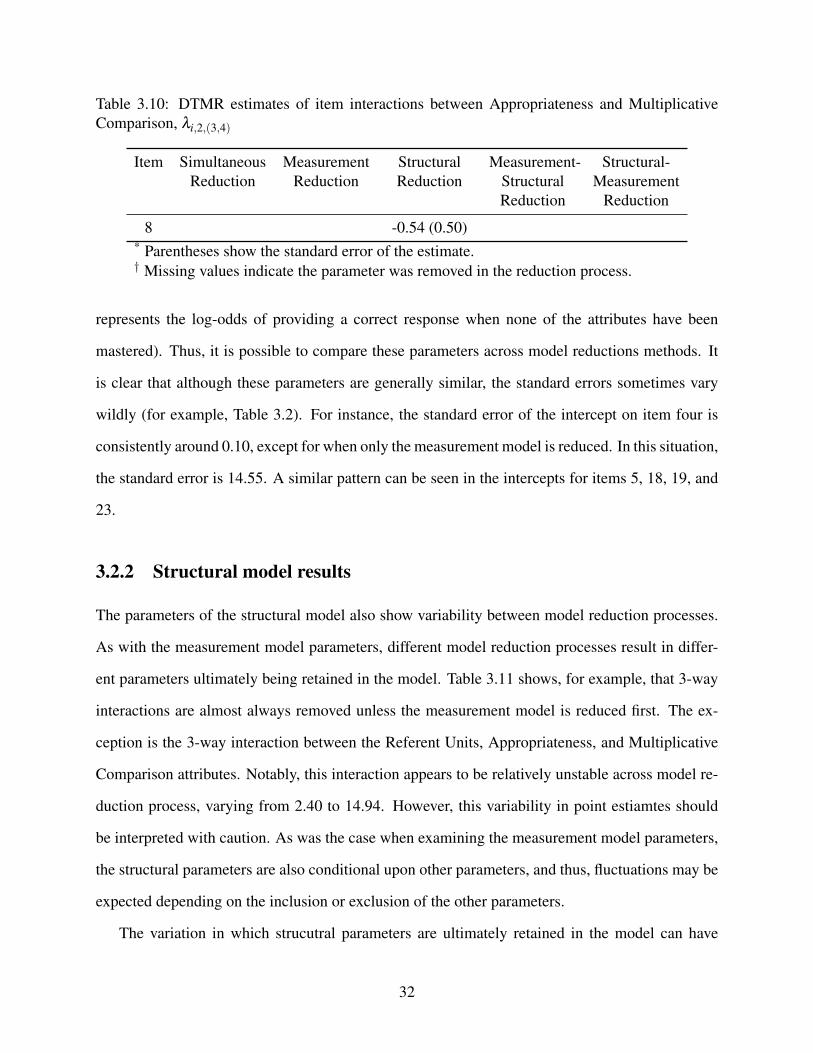
Table 3.10: DTMR estimates of item interactions between Appropriateness and MultiplicativeComparison, λi,2,(3,4)
Item SimultaneousReduction
MeasurementReduction
StructuralReduction
Measurement-StructuralReduction
Structural-Measurement
Reduction
8 -0.54 (0.50)* Parentheses show the standard error of the estimate.† Missing values indicate the parameter was removed in the reduction process.
represents the log-odds of providing a correct response when none of the attributes have been
mastered). Thus, it is possible to compare these parameters across model reductions methods. It
is clear that although these parameters are generally similar, the standard errors sometimes vary
wildly (for example, Table 3.2). For instance, the standard error of the intercept on item four is
consistently around 0.10, except for when only the measurement model is reduced. In this situation,
the standard error is 14.55. A similar pattern can be seen in the intercepts for items 5, 18, 19, and
23.
3.2.2 Structural model results
The parameters of the structural model also show variability between model reduction processes.
As with the measurement model parameters, different model reduction processes result in differ-
ent parameters ultimately being retained in the model. Table 3.11 shows, for example, that 3-way
interactions are almost always removed unless the measurement model is reduced first. The ex-
ception is the 3-way interaction between the Referent Units, Appropriateness, and Multiplicative
Comparison attributes. Notably, this interaction appears to be relatively unstable across model re-
duction process, varying from 2.40 to 14.94. However, this variability in point estiamtes should
be interpreted with caution. As was the case when examining the measurement model parameters,
the structural parameters are also conditional upon other parameters, and thus, fluctuations may be
expected depending on the inclusion or exclusion of the other parameters.
The variation in which strucutral parameters are ultimately retained in the model can have
32
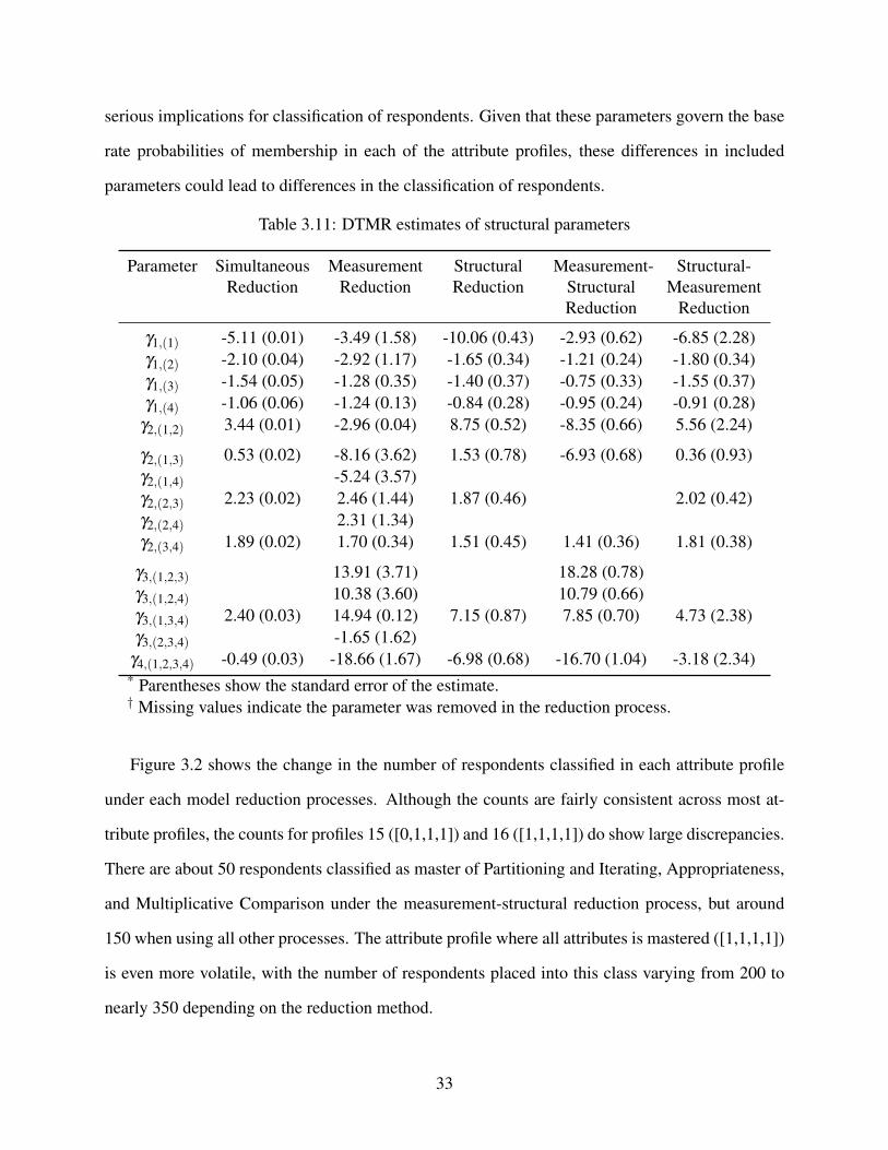
serious implications for classification of respondents. Given that these parameters govern the base
rate probabilities of membership in each of the attribute profiles, these differences in included
parameters could lead to differences in the classification of respondents.
Table 3.11: DTMR estimates of structural parameters
Parameter SimultaneousReduction
MeasurementReduction
StructuralReduction
Measurement-StructuralReduction
Structural-Measurement
Reduction
γ1,(1) -5.11 (0.01) -3.49 (1.58) -10.06 (0.43) -2.93 (0.62) -6.85 (2.28)γ1,(2) -2.10 (0.04) -2.92 (1.17) -1.65 (0.34) -1.21 (0.24) -1.80 (0.34)γ1,(3) -1.54 (0.05) -1.28 (0.35) -1.40 (0.37) -0.75 (0.33) -1.55 (0.37)γ1,(4) -1.06 (0.06) -1.24 (0.13) -0.84 (0.28) -0.95 (0.24) -0.91 (0.28)
γ2,(1,2) 3.44 (0.01) -2.96 (0.04) 8.75 (0.52) -8.35 (0.66) 5.56 (2.24)
γ2,(1,3) 0.53 (0.02) -8.16 (3.62) 1.53 (0.78) -6.93 (0.68) 0.36 (0.93)γ2,(1,4) -5.24 (3.57)γ2,(2,3) 2.23 (0.02) 2.46 (1.44) 1.87 (0.46) 2.02 (0.42)γ2,(2,4) 2.31 (1.34)γ2,(3,4) 1.89 (0.02) 1.70 (0.34) 1.51 (0.45) 1.41 (0.36) 1.81 (0.38)
γ3,(1,2,3) 13.91 (3.71) 18.28 (0.78)γ3,(1,2,4) 10.38 (3.60) 10.79 (0.66)γ3,(1,3,4) 2.40 (0.03) 14.94 (0.12) 7.15 (0.87) 7.85 (0.70) 4.73 (2.38)γ3,(2,3,4) -1.65 (1.62)
γ4,(1,2,3,4) -0.49 (0.03) -18.66 (1.67) -6.98 (0.68) -16.70 (1.04) -3.18 (2.34)* Parentheses show the standard error of the estimate.† Missing values indicate the parameter was removed in the reduction process.
Figure 3.2 shows the change in the number of respondents classified in each attribute profile
under each model reduction processes. Although the counts are fairly consistent across most at-
tribute profiles, the counts for profiles 15 ([0,1,1,1]) and 16 ([1,1,1,1]) do show large discrepancies.
There are about 50 respondents classified as master of Partitioning and Iterating, Appropriateness,
and Multiplicative Comparison under the measurement-structural reduction process, but around
150 when using all other processes. The attribute profile where all attributes is mastered ([1,1,1,1])
is even more volatile, with the number of respondents placed into this class varying from 200 to
nearly 350 depending on the reduction method.
33
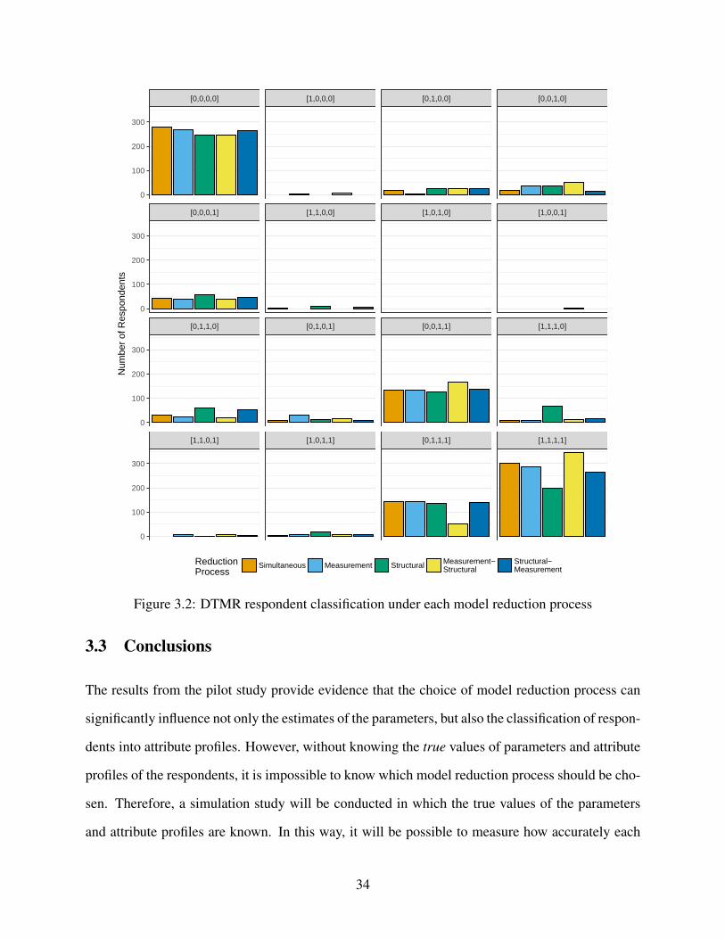
[1,1,0,1] [1,0,1,1] [0,1,1,1] [1,1,1,1]
[0,1,1,0] [0,1,0,1] [0,0,1,1] [1,1,1,0]
[0,0,0,1] [1,1,0,0] [1,0,1,0] [1,0,0,1]
[0,0,0,0] [1,0,0,0] [0,1,0,0] [0,0,1,0]
0
100
200
300
0
100
200
300
0
100
200
300
0
100
200
300
Num
ber
of R
espo
nden
ts
ReductionProcess
Simultaneous Measurement Structural Measurement−Structural
Structural−Measurement
Figure 3.2: DTMR respondent classification under each model reduction process
3.3 Conclusions
The results from the pilot study provide evidence that the choice of model reduction process can
significantly influence not only the estimates of the parameters, but also the classification of respon-
dents into attribute profiles. However, without knowing the true values of parameters and attribute
profiles of the respondents, it is impossible to know which model reduction process should be cho-
sen. Therefore, a simulation study will be conducted in which the true values of the parameters
and attribute profiles are known. In this way, it will be possible to measure how accurately each
34

model reduction process is able to recover parameter values and respondent attribute profiles. The
results of the simulation will then be able to inform which method is best suited to analyze the
DTMR data.
35
Chapter 4
Methods
The current study investigates the performance of the different model reduction processes using a
Monte Carlo simulation. The simulation will be designed to follow the structure and characteristics
of the DTMR data and the corresponding estimated parameters.
4.1 Overview of Monte Carlo methods
Broadly speaking, Monte Carlo simulations can be used to evaluate the performance of different or
competing methodologies (Rubinstein & Kroese, 2017). As discussed in section 3.3, when using
real data it is difficult to evaluate competing procedures, because the true values of the parameters
are unknown. Thus, the estimates from different procedures can be compared to each other, but
cannot be compared to what the real value is. With Monte Carlo methods, data is generated from
a model with known parameters. The different procedures can be used on the simulated data, and
then the resulting estimates compared to the actual values that were used to generate the data.
The general process of a Monte Carlo simulation is as follows:
1. Define distributions for model parameters,
2. Randomly draw model parameters from previously defined distributions,
3. Simulate response data from the drawn model parameters,
4. Estimate the model using simulated response data, and
5. Compare estimated parameters to the parameters that were randomly drawn and used to
simulate the data.
36
Monte Carlo studies have been used extensively in psychometric research (see Feinberg &
Rubright, 2016 for a survey of simulation studies in educational measurement). There are disad-
vantages to this methodology however (e.g., Harwell, Stone, Hsu, & Kirisci, 1996). In the simu-
lation of data, only parameters that are defined influence the generation of response data. Thus, if
the model specified in the simulation study is inconsistent with reality, the simulation may not be
informative. Additionally, the data generated will be perfectly model fitting (unless misfit is intro-
duced in the data generation process). This means that the findings of the simulation study may not
hold when there is misfit in the data. In other words, the main disadvantage of Monte Carlo studies
is that simulation environment may not generalize to empirical data. Therefore, when designing a
Monte Carlo study it is important to make the conditions and parameter distributions as realistic as
possible (Feinberg & Rubright, 2016).
4.2 The current simulation
In order to make this simulation as realistic as possible, it will be modeled after the DTMR assess-
ment and the results from the pilot study.
4.2.1 Simulation conditions
The DTMR assessment consists of 28 items measuring four attributes. The simulation study will
use three and four attributes in order to assess the effects of increasingly complex structural mod-
els. Additionally, each condition will hold the number of items constant at 30 to reduce the number
of conditions in the simulation. Three sample size conditions will be used: 500, 1000, and 5000.
These sizes are representative of hte DTMR sample size of 990, a smaller sample, and a large sam-
ple that would remove any sample size concerns for estimation. This will allows for the evaluation
of sample size effects. Thus, there are two attribute conditions times three sample size conditions
= six data generation conditions.
For each generated data set, three Q-matrices will be used to estimate the model: the true Q-
37
matrix, a 10 percent over-specified Q-matrix, and a 20 percent over-specified Q-matrix. In the
over-specified Q-matrices, each value of zero in the Q-matrix will have either a 10 or 20 percent
chance of being changed to a one, depending on the condition. Finally, for each Q-matrix, the
model will be estimated in six ways:
1. Saturated model,
2. Simultaneous reduction,
3. Measurement reduction,
4. Structural reduction,
5. Measurement-Structural reduction, and
6. Structural-Measurement reduction.
This results in a total of three Q-matrix conditions times six model estimation conditions =
18 estimation conditions. Therefore, there are six data generation conditions times 18 estimation
conditions = 108 total conditions. Each condition will be replicated 100 times to ensure that robust
estimates of the outcomes measures can be calculated for each condition.
4.2.2 Data generation process
When simulating data sets, the γ parameters that make up the structural model will be simulated
first. There are no constraints on the values of γ; however, based on the results of the pilot study,
structural parameters will be drawn from a N (0,2) distribution. Using this distribution, most
draws will come within 3 standard deviations of the mean, resulting in most values falling between
-6 and 6. These values are consistent with what is seen in the DTMR pilot study (Table 3.11).
Additionally, this range allows for large effects using the guidelines suggest by Chinn (2000), but
also makes very large γ values unlikely.
Once the structural parameters have been generated, the base rate probabilities for each class
can be calculated. These will in turn be used to generate attribute profiles for the simulated re-
spondents. The attribute profiles, in conjunctions with item parameters, are used to calculate the
38
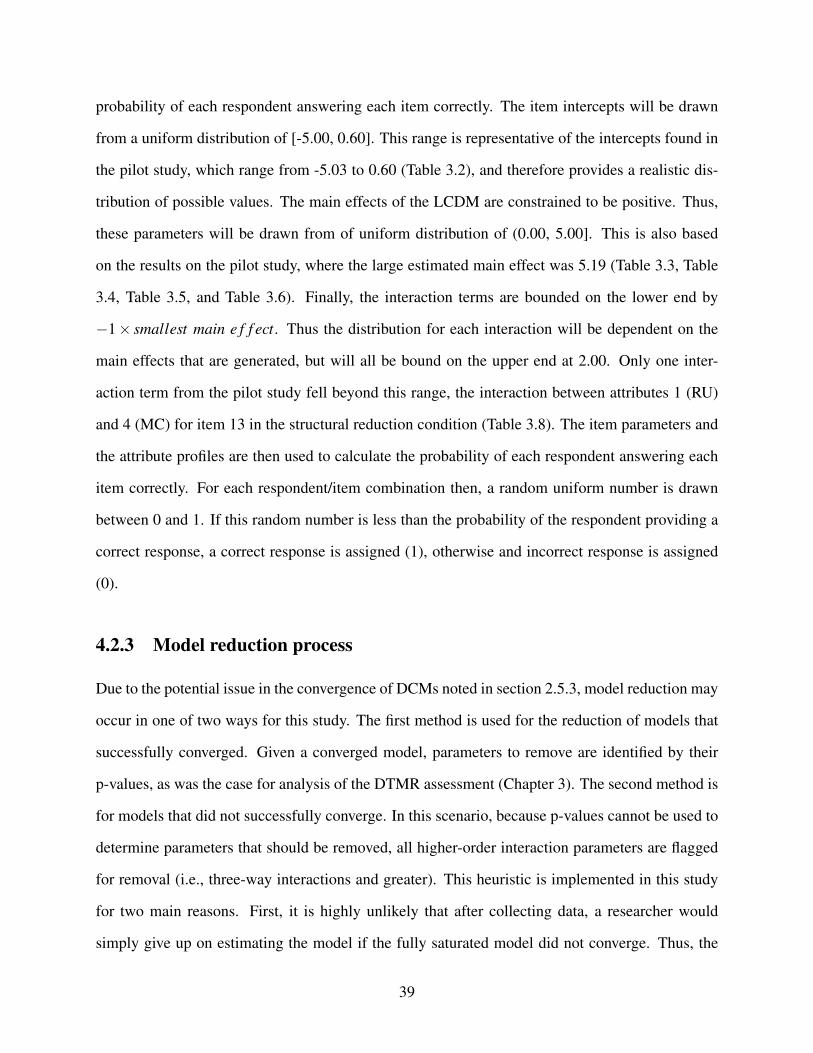
probability of each respondent answering each item correctly. The item intercepts will be drawn
from a uniform distribution of [-5.00, 0.60]. This range is representative of the intercepts found in
the pilot study, which range from -5.03 to 0.60 (Table 3.2), and therefore provides a realistic dis-
tribution of possible values. The main effects of the LCDM are constrained to be positive. Thus,
these parameters will be drawn from of uniform distribution of (0.00, 5.00]. This is also based
on the results on the pilot study, where the large estimated main effect was 5.19 (Table 3.3, Table
3.4, Table 3.5, and Table 3.6). Finally, the interaction terms are bounded on the lower end by
−1× smallest main e f f ect. Thus the distribution for each interaction will be dependent on the
main effects that are generated, but will all be bound on the upper end at 2.00. Only one inter-
action term from the pilot study fell beyond this range, the interaction between attributes 1 (RU)
and 4 (MC) for item 13 in the structural reduction condition (Table 3.8). The item parameters and
the attribute profiles are then used to calculate the probability of each respondent answering each
item correctly. For each respondent/item combination then, a random uniform number is drawn
between 0 and 1. If this random number is less than the probability of the respondent providing a
correct response, a correct response is assigned (1), otherwise and incorrect response is assigned
(0).
4.2.3 Model reduction process
Due to the potential issue in the convergence of DCMs noted in section 2.5.3, model reduction may
occur in one of two ways for this study. The first method is used for the reduction of models that
successfully converged. Given a converged model, parameters to remove are identified by their
p-values, as was the case for analysis of the DTMR assessment (Chapter 3). The second method is
for models that did not successfully converge. In this scenario, because p-values cannot be used to
determine parameters that should be removed, all higher-order interaction parameters are flagged
for removal (i.e., three-way interactions and greater). This heuristic is implemented in this study
for two main reasons. First, it is highly unlikely that after collecting data, a researcher would
simply give up on estimating the model if the fully saturated model did not converge. Thus, the
39
inclusion of this rule-based model reduction will inform practitioners on best practices. Secondly,
the removal of higher-order interaction terms has already been implemented in the literature as a
method for dealing with non-convergence (see Bradshaw et al., 2014 for an example). Accord-
ingly, this implementation of this rule in the simulation study mimics the current practice of model
estimation. A modifiied model reduction flow chart can be seen in Figure 4.1.
FullySaturated
SimultaneousReduction
MeasurementReduction
StructuralReduction
Measurement−StrucutralReduction
Structural−Measurement
Reduction
ReductionMethod
p−value Heuristic
Figure 4.1: Flowchart of simulation study reduction processes
Note that in Figure 4.1, the rule-based model reductions can only occur after the fully saturated
model. The logic behind this decision is as follows. If the fully saturated converges and the next
model fails to converge, the practitioner should revert back to the model that successfully con-
verged, rather than continuing to attempt to remove additional parameters. Conversely, if the fully
saturated model fails to converge, and the next model also fails to converge, then the third model
would result in the removal of both measurement and structural parameters using the heuristic.
This would then be equivalent to the simultaneous reduction method using the heuristic, rendering
third-step model redundant. Finally, regardless of the convergance of the fully saturated model, if
40
the second-step model converges, the model reduction process can continue to the third step using
p-values.
4.2.4 Outcome measures
Results for models that were reduced from converged and non-converged models will be analyzed
separately. This is to allow for the possibility that different methods of reducing the model may
prefer different model reduction processes. Accordingly, convergence rates of each model reduc-
tion process will be an important outcome measure. In addition, estimated item and structural
parameters will be compared to the true values. The bias and mean squared error of the estimates
will be calculated to evaluate the ability of each model reduction process to recover the parameter
values. In these calculations, parameters that were removed in the reduction process will have their
estimates set to 0.
In addition to the recovery of model parameters, the recovery of attribute profiles will also be
examined. This will be calculated at both the attribute and pattern level. This distinction differen-
tiates how accurate attribute mastery was and how accurate profile assignment was. For example,
assume a respondent had a true attribute profile of [1,0,1,0], and an estimated profile of [1,1,1,0].
At the pattern level, they were incorrectly assigned to an attribute profile. However, at the attribute
level, 75% of attributes were correctly estimated. These measures will be evaluated using percent
correct classification, and the quadratically weighted Cohen’s kappa (Cohen, 1960, 1968).
Another important outcome of the model fitting process is model data fit. Thus, it is important
to investigate whether any reduction processes consistently provide better fit to the data. This will
be assessed using the Akaike information criterion (AIC; Akaike, 1974), Bayesian information
criterion (BIC; Schwarz, 1978), and the adjusted Bayesian information criterion (Sclove, 1987).
These methods all measure the relative fit of a model compared to competing models. All the
methods measure how well the model fits the data, with a penalty for the number of parameters.
Within each measure, the model with the lowest index on the measure is the preferred model,
taking into account both overall fit and model complexity.
41
Finally, diagnostics of the model reduction processes will be examined. Specifically, the rate at
which each process results in the correct parameters being retained in the model will be examined.
This will be examined separately for the measurement and structural models. Additionally, the
distributions of the values and standard errors of parameters that are reduced with p-values will be
evaluated. This will allow for an analysis of whether reduced parameters are being removed due
to small parameter estimates or overly large standard errors.
4.2.5 Software
As with the pilot study, all models were estimated using Mplus version 7.4 (L. K. Muthén &
Muthén, 1998) via the MplusAutomation package (Hallquist & Wiley, 2018) in R version 3.4.3
(R Core Team, 2017). Mplus code for the estimation of the LCDM was generated in R using
custom scripts based on the work of Rupp & Wilhelm (2012) and Templin & Hoffman (2013).
Data generation and evaluation of the models was carried out in R using the dplyr (Wickham,
Francois, Henry, & Müller, 2018), forcats (Wickham, 2018a), glue (Hester, 2017), lubridate
(Spinu, Grolemund, & Wickham, 2018), portableParallelSeeds (Johnson, 2016), purrr (Henry
& Wickham, 2017), readr (Wickham, Hester, & Francois, 2017), stringr (Wickham, 2018b),
tibble (Müller & Wickham, 2018), tidyr (Wickham & Henry, 2018), and tidyselect (Henry &
Wickham, 2018) packages. All analyses were carried out on the Amazon Elastic Compute Cloud
(EC2; Amazon Web Services, 2018).
42
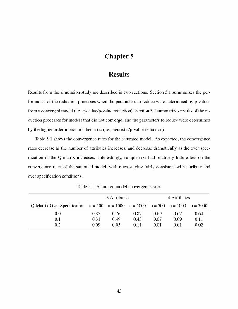
Chapter 5
Results
Results from the simulation study are described in two sections. Section 5.1 summarizes the per-
formance of the reduction processes when the parameters to reduce were determined by p-values
from a converged model (i.e., p-value/p-value reduction). Section 5.2 summarizes results of the re-
duction processes for models that did not converge, and the parameters to reduce were determined
by the higher order interaction heuristic (i.e., heuristic/p-value reduction).
Table 5.1 shows the convergence rates for the saturated model. As expected, the convergence
rates decrease as the number of attributes increases, and decrease dramatically as the over spec-
ification of the Q-matrix increases. Interestingly, sample size had relatively little effect on the
convergence rates of the saturated model, with rates staying fairly consistent with attribute and
over specification conditions.
Table 5.1: Saturated model convergence rates
3 Attributes 4 Attributes
Q-Matrix Over Specification n = 500 n = 1000 n = 5000 n = 500 n = 1000 n = 5000
0.0 0.85 0.76 0.87 0.69 0.67 0.640.1 0.31 0.49 0.43 0.07 0.09 0.110.2 0.09 0.05 0.11 0.01 0.01 0.02
43
5.1 Reduction by p-value
5.1.1 Convergence
When saturated model converged, reduction of measurement and structural parameters proceeded
by using p-values to determine which parameters to reduce. Figure 5.1 shows the convergence
rates for these reduction processes when the saturated model converged. Recall that measurement-
structural and structural measurement reduction only occurred if the measurement and structural
reductions, respectively, converged. Across all conditions, reduction processes where there mea-
surement model was reduced first (i.e., simultaneous, measurement, and measurement-structural)
tended to have higher convergence rates. This was most notable when the Q-matrix was over
specified. In the most extreme case, the four-attribute condition with a 20 percent over specified
Q-matrix, no reductions converged if the measurement model was not part of the initial reduction.
However, because the saturated model very rarely converged for this condition (Table 5.1), the
sample size is very limited.
44
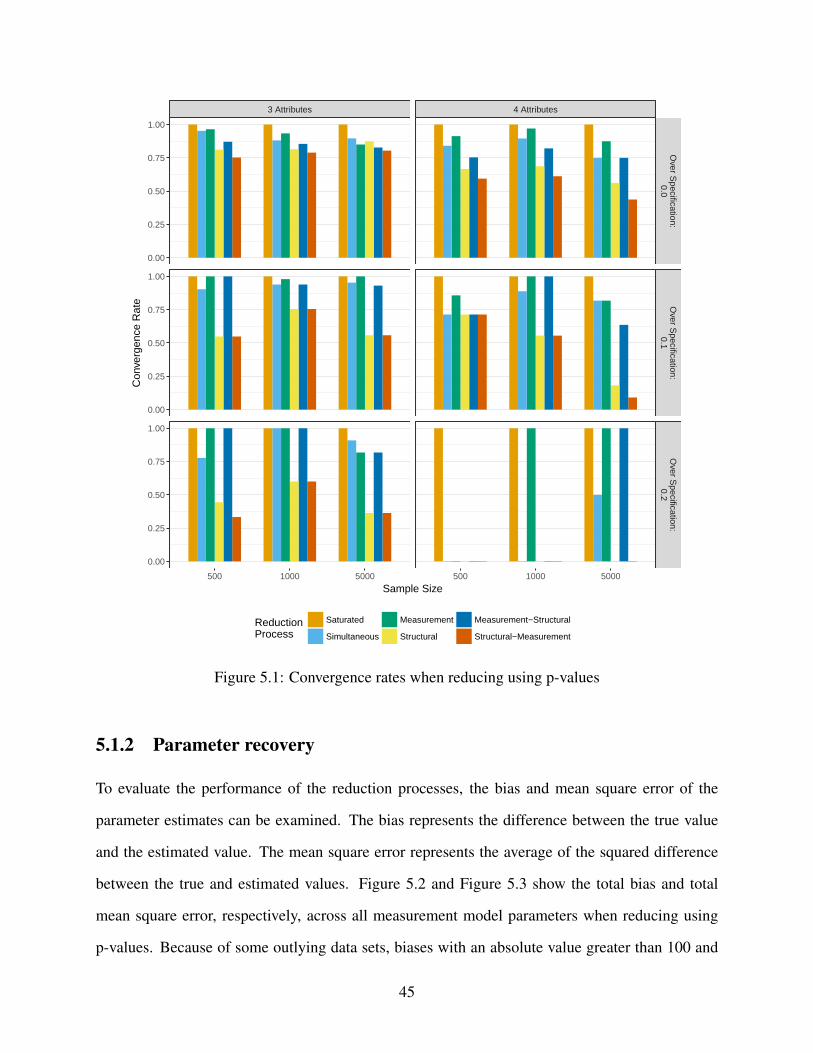
3 Attributes 4 Attributes
Over S
pecification:0.0
Over S
pecification:0.1
Over S
pecification:0.2
500 1000 5000 500 1000 5000
0.00
0.25
0.50
0.75
1.00
0.00
0.25
0.50
0.75
1.00
0.00
0.25
0.50
0.75
1.00
Sample Size
Con
verg
ence
Rat
e
ReductionProcess
Saturated
Simultaneous
Measurement
Structural
Measurement−Structural
Structural−Measurement
Figure 5.1: Convergence rates when reducing using p-values
5.1.2 Parameter recovery
To evaluate the performance of the reduction processes, the bias and mean square error of the
parameter estimates can be examined. The bias represents the difference between the true value
and the estimated value. The mean square error represents the average of the squared difference
between the true and estimated values. Figure 5.2 and Figure 5.3 show the total bias and total
mean square error, respectively, across all measurement model parameters when reducing using
p-values. Because of some outlying data sets, biases with an absolute value greater than 100 and
45
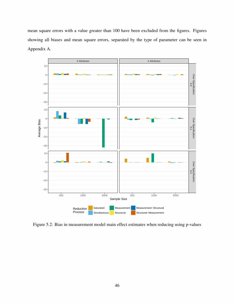
mean square errors with a value greater than 100 have been excluded from the figures. Figures
showing all biases and mean square errors, separated by the type of parameter can be seen in
Appendix A.
3 Attributes 4 Attributes
Over S
pecification:0.0
Over S
pecification:0.1
Over S
pecification:0.2
500 1000 5000 500 1000 5000
−30
−20
−10
0
10
−30
−20
−10
0
10
−30
−20
−10
0
10
Sample Size
Ave
rage
Bia
s
ReductionProcess
Saturated
Simultaneous
Measurement
Structural
Measurement−Structural
Structural−Measurement
Figure 5.2: Bias in measurement model main effect estimates when reducing using p-values
46
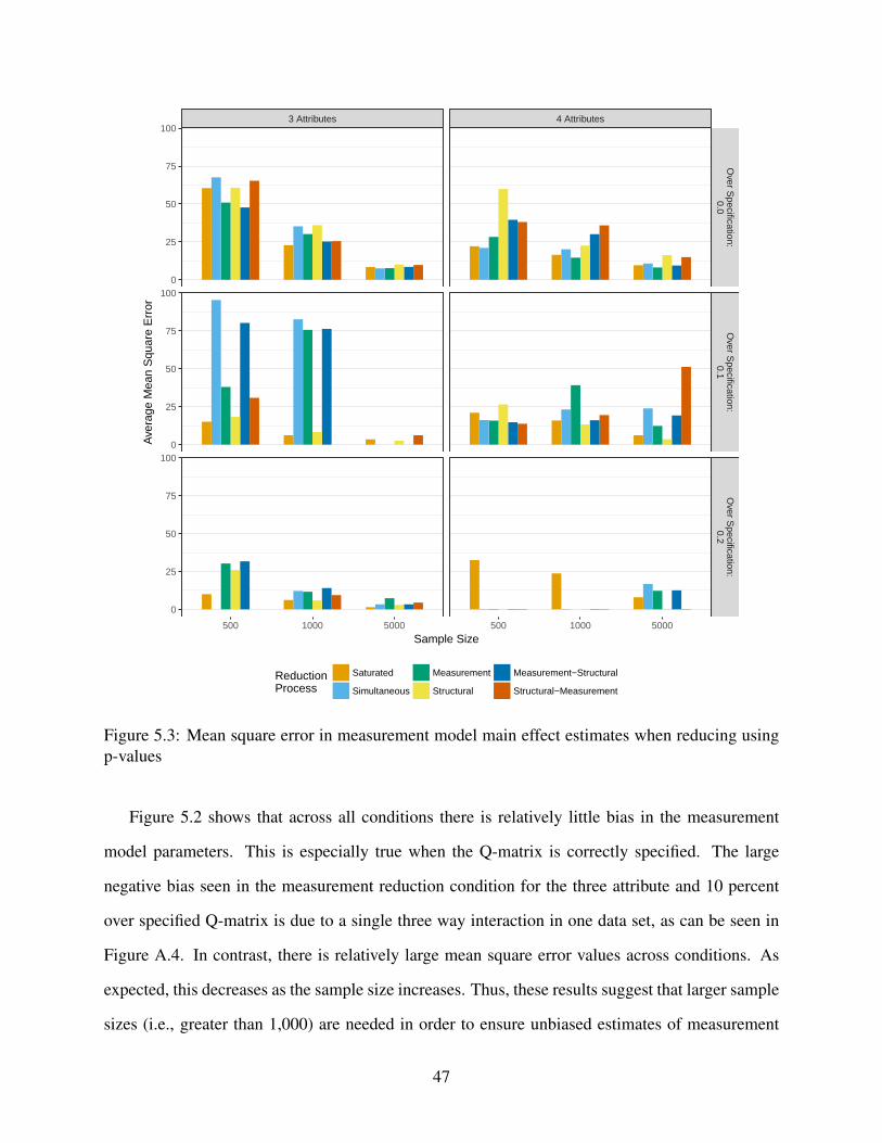
3 Attributes 4 Attributes
Over S
pecification:0.0
Over S
pecification:0.1
Over S
pecification:0.2
500 1000 5000 500 1000 5000
0
25
50
75
100
0
25
50
75
100
0
25
50
75
100
Sample Size
Ave
rage
Mea
n S
quar
e E
rror
ReductionProcess
Saturated
Simultaneous
Measurement
Structural
Measurement−Structural
Structural−Measurement
Figure 5.3: Mean square error in measurement model main effect estimates when reducing usingp-values
Figure 5.2 shows that across all conditions there is relatively little bias in the measurement
model parameters. This is especially true when the Q-matrix is correctly specified. The large
negative bias seen in the measurement reduction condition for the three attribute and 10 percent
over specified Q-matrix is due to a single three way interaction in one data set, as can be seen in
Figure A.4. In contrast, there is relatively large mean square error values across conditions. As
expected, this decreases as the sample size increases. Thus, these results suggest that larger sample
sizes (i.e., greater than 1,000) are needed in order to ensure unbiased estimates of measurement
47
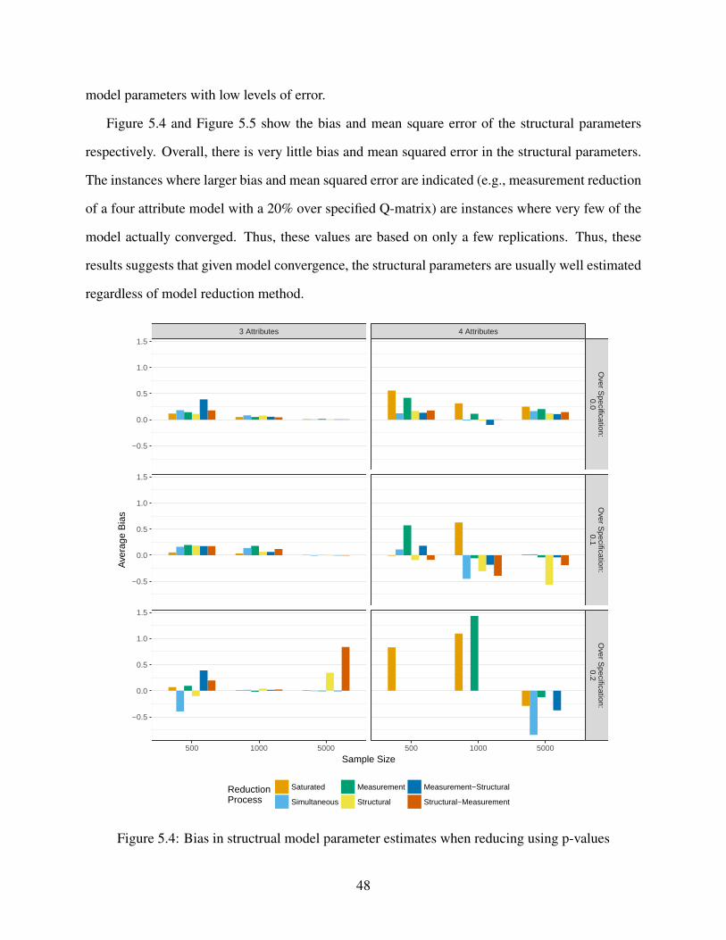
model parameters with low levels of error.
Figure 5.4 and Figure 5.5 show the bias and mean square error of the structural parameters
respectively. Overall, there is very little bias and mean squared error in the structural parameters.
The instances where larger bias and mean squared error are indicated (e.g., measurement reduction
of a four attribute model with a 20% over specified Q-matrix) are instances where very few of the
model actually converged. Thus, these values are based on only a few replications. Thus, these
results suggests that given model convergence, the structural parameters are usually well estimated
regardless of model reduction method.
3 Attributes 4 Attributes
Over S
pecification:0.0
Over S
pecification:0.1
Over S
pecification:0.2
500 1000 5000 500 1000 5000
−0.5
0.0
0.5
1.0
1.5
−0.5
0.0
0.5
1.0
1.5
−0.5
0.0
0.5
1.0
1.5
Sample Size
Ave
rage
Bia
s
ReductionProcess
Saturated
Simultaneous
Measurement
Structural
Measurement−Structural
Structural−Measurement
Figure 5.4: Bias in structrual model parameter estimates when reducing using p-values
48
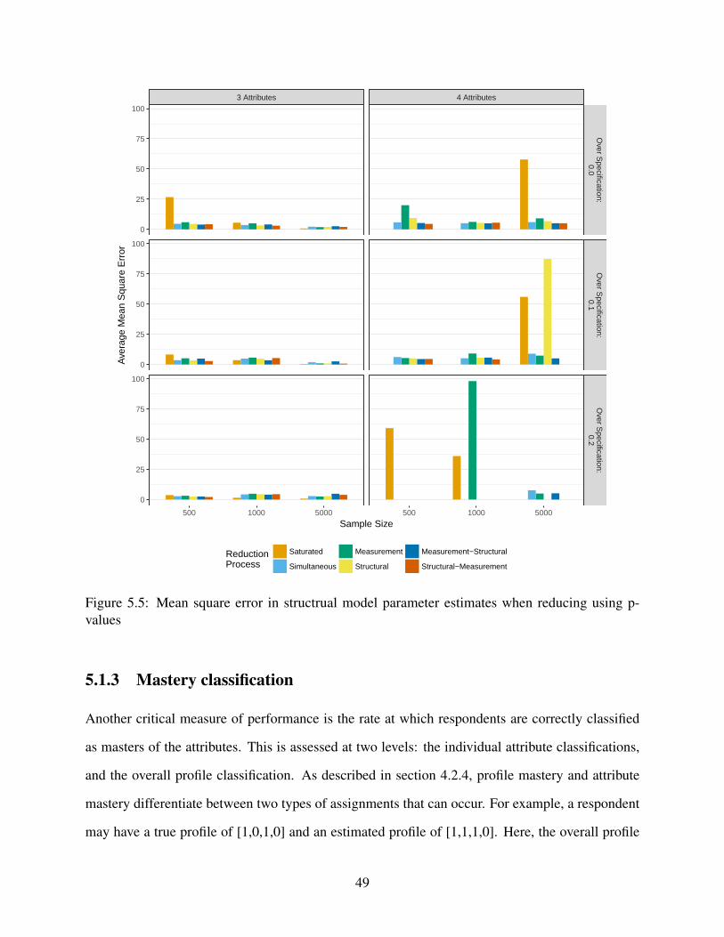
3 Attributes 4 Attributes
Over S
pecification:0.0
Over S
pecification:0.1
Over S
pecification:0.2
500 1000 5000 500 1000 5000
0
25
50
75
100
0
25
50
75
100
0
25
50
75
100
Sample Size
Ave
rage
Mea
n S
quar
e E
rror
ReductionProcess
Saturated
Simultaneous
Measurement
Structural
Measurement−Structural
Structural−Measurement
Figure 5.5: Mean square error in structrual model parameter estimates when reducing using p-values
5.1.3 Mastery classification
Another critical measure of performance is the rate at which respondents are correctly classified
as masters of the attributes. This is assessed at two levels: the individual attribute classifications,
and the overall profile classification. As described in section 4.2.4, profile mastery and attribute
mastery differentiate between two types of assignments that can occur. For example, a respondent
may have a true profile of [1,0,1,0] and an estimated profile of [1,1,1,0]. Here, the overall profile
49

assignment is incorrect (profile classification), but three out of the four individual attributes are
correctly classified (attribute classification). Respondents were classified as a master of an attribute
if their posterior probability of mastery was greater than or equal to .5, and non-master of the
attribute otherwise. Figure 5.6 and Figure 5.7 show the attribute level agreement as measured by
the average correct classification rate and average Cohen’s κ , respectively.
3 Attributes 4 Attributes
Over S
pecification:0.0
Over S
pecification:0.1
Over S
pecification:0.2
500 1000 5000 500 1000 5000
0.00
0.25
0.50
0.75
1.00
0.00
0.25
0.50
0.75
1.00
0.00
0.25
0.50
0.75
1.00
Sample Size
Attr
ibut
e C
orre
ct C
lass
ifica
tion
Rat
e
ReductionProcess
Saturated
Simultaneous
Measurement
Structural
Measurement−Structural
Structural−Measurement
Figure 5.6: Average correct classification rate of attribute mastery when reducing using p-values
50
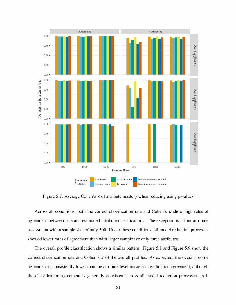
3 Attributes 4 Attributes
Over S
pecification:0.0
Over S
pecification:0.1
Over S
pecification:0.2
500 1000 5000 500 1000 5000
0.00
0.25
0.50
0.75
1.00
0.00
0.25
0.50
0.75
1.00
0.00
0.25
0.50
0.75
1.00
Sample Size
Ave
rage
Attr
ibut
e C
ohen
's κ
ReductionProcess
Saturated
Simultaneous
Measurement
Structural
Measurement−Structural
Structural−Measurement
Figure 5.7: Average Cohen’s κ of attribute mastery when reducing using p-values
Across all conditions, both the correct classification rate and Cohen’s κ show high rates of
agreement between true and estimated attribute classifications. The exception is a four-attribute
assessment with a sample size of only 500. Under these conditions, all model reduction processes
showed lower rates of agreement than with larger samples or only three attributes.
The overall profile classification shows a similar pattern. Figure 5.8 and Figure 5.9 show the
correct classification rate and Cohen’s κ of the overall profiles. As expected, the overall profile
agreement is consistently lower than the attribute level mastery classification agreement, although
the classification agreement is generally consistent across all model reduction processes. Ad-
51
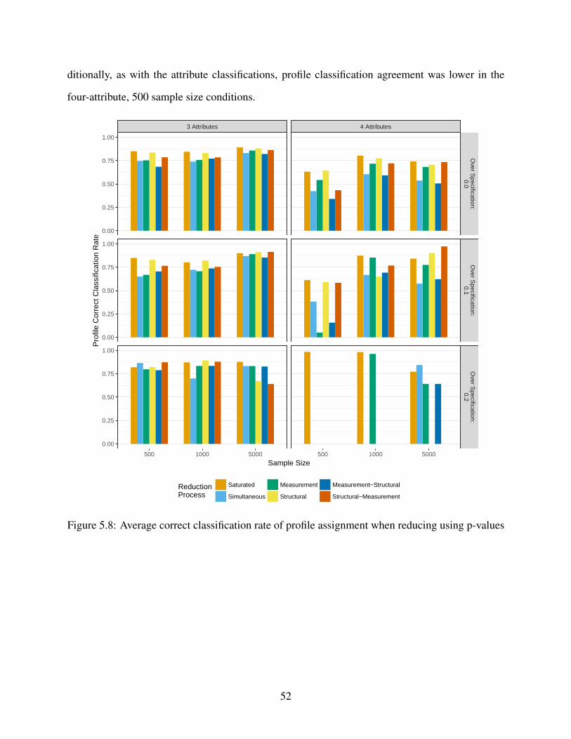
ditionally, as with the attribute classifications, profile classification agreement was lower in the
four-attribute, 500 sample size conditions.
3 Attributes 4 Attributes
Over S
pecification:0.0
Over S
pecification:0.1
Over S
pecification:0.2
500 1000 5000 500 1000 5000
0.00
0.25
0.50
0.75
1.00
0.00
0.25
0.50
0.75
1.00
0.00
0.25
0.50
0.75
1.00
Sample Size
Pro
file
Cor
rect
Cla
ssifi
catio
n R
ate
ReductionProcess
Saturated
Simultaneous
Measurement
Structural
Measurement−Structural
Structural−Measurement
Figure 5.8: Average correct classification rate of profile assignment when reducing using p-values
52
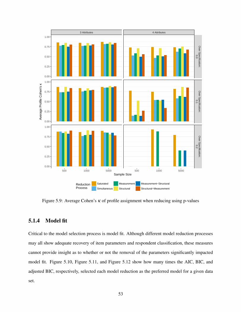
3 Attributes 4 Attributes
Over S
pecification:0.0
Over S
pecification:0.1
Over S
pecification:0.2
500 1000 5000 500 1000 5000
0.00
0.25
0.50
0.75
1.00
0.00
0.25
0.50
0.75
1.00
0.00
0.25
0.50
0.75
1.00
Sample Size
Ave
rage
Pro
file
Coh
en's
κ
ReductionProcess
Saturated
Simultaneous
Measurement
Structural
Measurement−Structural
Structural−Measurement
Figure 5.9: Average Cohen’s κ of profile assignment when reducing using p-values
5.1.4 Model fit
Critical to the model selection process is model fit. Although different model reduction processes
may all show adequate recovery of item parameters and respondent classification, these measures
cannot provide insight as to whether or not the removal of the parameters significantly impacted
model fit. Figure 5.10, Figure 5.11, and Figure 5.12 show how many times the AIC, BIC, and
adjusted BIC, respectively, selected each model reduction as the preferred model for a given data
set.
53
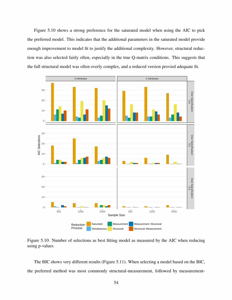
Figure 5.10 shows a strong preference for the saturated model when using the AIC to pick
the preferred model. This indicates that the additional parameters in the saturated model provide
enough improvement to model fit to justify the additional complexity. However, structural reduc-
tion was also selected fairly often, especially in the true Q-matrix conditions. This suggests that
the full structural model was often overly complex, and a reduced version provied adequate fit.
3 Attributes 4 Attributes
Over S
pecification:0.0
Over S
pecification:0.1
Over S
pecification:0.2
500 1000 5000 500 1000 5000
0
10
20
30
0
10
20
30
0
10
20
30
Sample Size
AIC
Sel
ectio
ns
ReductionProcess
Saturated
Simultaneous
Measurement
Structural
Measurement−Structural
Structural−Measurement
Figure 5.10: Number of selections as best fitting model as measured by the AIC when reducingusing p-values
The BIC shows very different results (Figure 5.11). When selecting a model based on the BIC,
the preferred method was most commonly structural-measurement, followed by measurement-
54
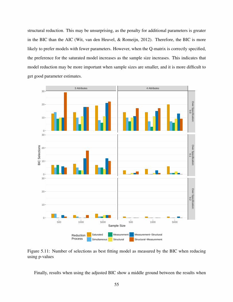
structural reduction. This may be unsurprising, as the penalty for additional parameters is greater
in the BIC than the AIC (Wit, van den Heuvel, & Romeijn, 2012). Therefore, the BIC is more
likely to prefer models with fewer parameters. However, when the Q-matrix is correctly specified,
the preference for the saturated model increases as the sample size increases. This indicates that
model reduction may be more important when sample sizes are smaller, and it is more difficult to
get good parameter estimates.
3 Attributes 4 Attributes
Over S
pecification:0.0
Over S
pecification:0.1
Over S
pecification:0.2
500 1000 5000 500 1000 5000
0
10
20
30
0
10
20
30
0
10
20
30
Sample Size
BIC
Sel
ectio
ns
ReductionProcess
Saturated
Simultaneous
Measurement
Structural
Measurement−Structural
Structural−Measurement
Figure 5.11: Number of selections as best fitting model as measured by the BIC when reducingusing p-values
Finally, results when using the adjusted BIC show a middle ground between the results when
55
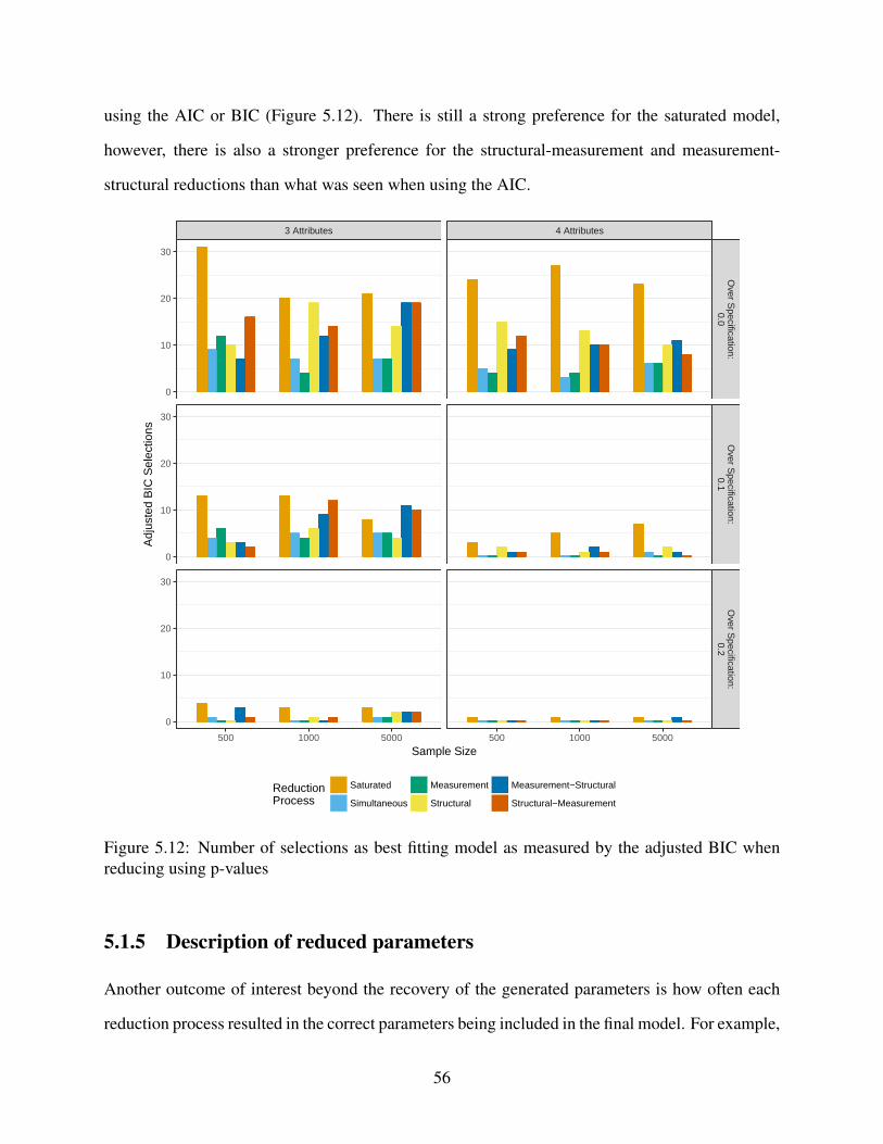
using the AIC or BIC (Figure 5.12). There is still a strong preference for the saturated model,
however, there is also a stronger preference for the structural-measurement and measurement-
structural reductions than what was seen when using the AIC.
3 Attributes 4 Attributes
Over S
pecification:0.0
Over S
pecification:0.1
Over S
pecification:0.2
500 1000 5000 500 1000 5000
0
10
20
30
0
10
20
30
0
10
20
30
Sample Size
Adj
uste
d B
IC S
elec
tions
ReductionProcess
Saturated
Simultaneous
Measurement
Structural
Measurement−Structural
Structural−Measurement
Figure 5.12: Number of selections as best fitting model as measured by the adjusted BIC whenreducing using p-values
5.1.5 Description of reduced parameters
Another outcome of interest beyond the recovery of the generated parameters is how often each
reduction process resulted in the correct parameters being included in the final model. For example,
56
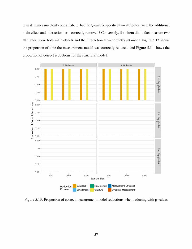
if an item measured only one attribute, but the Q-matrix specified two attributes, were the additional
main effect and interaction term correctly removed? Conversely, if an item did in fact measure two
attributes, were both main effects and the interaction term correctly retained? Figure 5.13 shows
the proportion of time the measurement model was correctly reduced, and Figure 5.14 shows the
proportion of correct reductions for the structural model.
3 Attributes 4 Attributes
Over S
pecification:0.0
Over S
pecification:0.1
Over S
pecification:0.2
500 1000 5000 500 1000 5000
0.00
0.25
0.50
0.75
1.00
0.00
0.25
0.50
0.75
1.00
0.00
0.25
0.50
0.75
1.00
Sample Size
Pro
post
ion
of C
orre
ct R
educ
tions
ReductionProcess
Saturated
Simultaneous
Measurement
Structural
Measurement−Structural
Structural−Measurement
Figure 5.13: Proportion of correct measurement model reductions when reducing with p-values
57
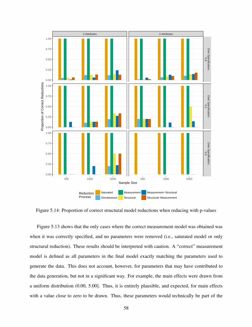
3 Attributes 4 Attributes
Over S
pecification:0.0
Over S
pecification:0.1
Over S
pecification:0.2
500 1000 5000 500 1000 5000
0.00
0.25
0.50
0.75
1.00
0.00
0.25
0.50
0.75
1.00
0.00
0.25
0.50
0.75
1.00
Sample Size
Pro
port
ion
of C
orre
ct R
educ
tions
ReductionProcess
Saturated
Simultaneous
Measurement
Structural
Measurement−Structural
Structural−Measurement
Figure 5.14: Proportion of correct structural model reductions when reducing with p-values
Figure 5.13 shows that the only cases where the correct measurement model was obtained was
when it was correctly specified, and no parameters were removed (i.e., saturated model or only
structural reduction). These results should be interpreted with caution. A “correct” measurement
model is defined as all parameters in the final model exactly matching the parameters used to
generate the data. This does not account, however, for parameters that may have contributed to
the data generation, but not in a significant way. For example, the main effects were drawn from
a uniform distribution (0.00, 5.00]. Thus, it is entirely plausible, and expected, for main effects
with a value close to zero to be drawn. Thus, these parameters would technically be part of the
58
true measurement model, but may not be statistically significant, and even one of these parameters
would result in the determination of an incorrect measurement model.
A similar pattern is seen in Figure 5.14, with very low rates of correct reduction, except when
no reduction of the structural model was performed (i.e., saturated model or only measurement
reduction). Because the data was always generated with a fully saturated log-linear structural
model, and reduction of the structural model results in a determination of an incorrect reduction.
However, given that the structural parameters were all drawn from a N (0,2) distribution the same
caveats of significance apply that applied to the measurement model parameters.
To verify that the parameters being reduced are indeed these parameters that are very small,
and thus may not be significant, the distributions of estimates and standard errors of the reduced
parameters can be examined. Figure 5.15 shows that the majority of reduced measurement model
parameters are small in value, with small standard errors. More parameters were removed from the
true Q-matrix conditions than the over specified Q-matrix conditions, however this is an artifact of
the over specified conditions converging far less often.
Figure 5.16 shows a similar pattern for the structural parameters, with the majority of reduced
parameters having an estimate close to zero. Additionally, the most of the reduction occurred
out of the true Q-matrix conditions, as the over specification conditions often failed to converge.
However, unlike the measurement model parameters, there is more variability in the estimates and
standard errors of the parameters that were reduced.
59
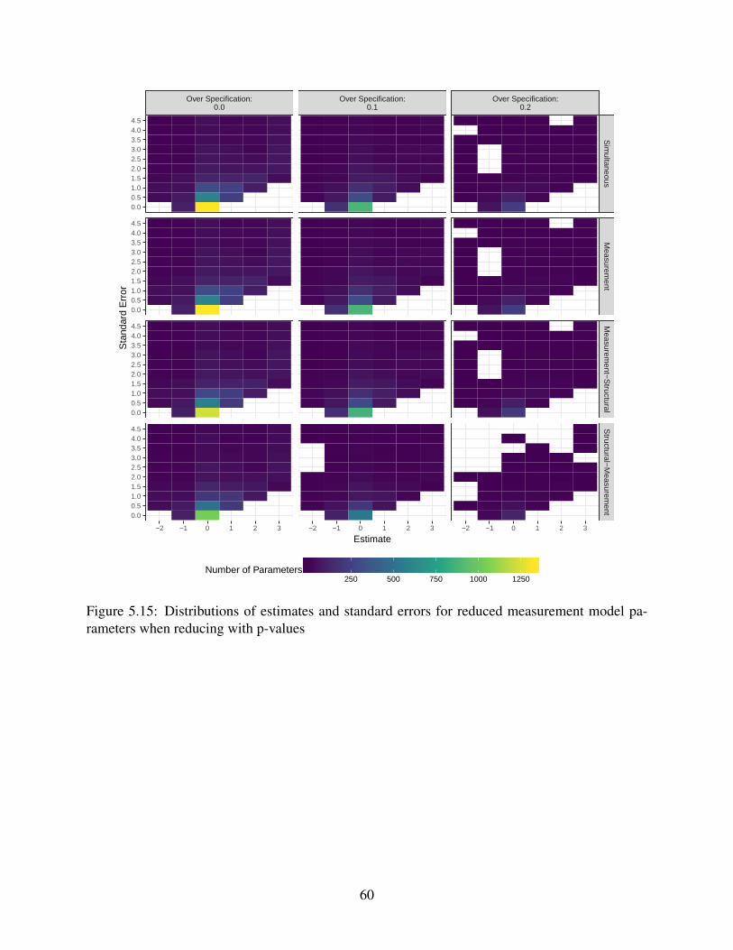
Over Specification:0.0
Over Specification:0.1
Over Specification:0.2
Sim
ultaneousM
easurement
Measurem
ent−S
tructuralS
tructural−M
easurement
−2 −1 0 1 2 3 −2 −1 0 1 2 3 −2 −1 0 1 2 3
0.00.51.01.52.02.53.03.54.04.5
0.00.51.01.52.02.53.03.54.04.5
0.00.51.01.52.02.53.03.54.04.5
0.00.51.01.52.02.53.03.54.04.5
Estimate
Sta
ndar
d E
rror
250 500 750 1000 1250Number of Parameters
Figure 5.15: Distributions of estimates and standard errors for reduced measurement model pa-rameters when reducing with p-values
60
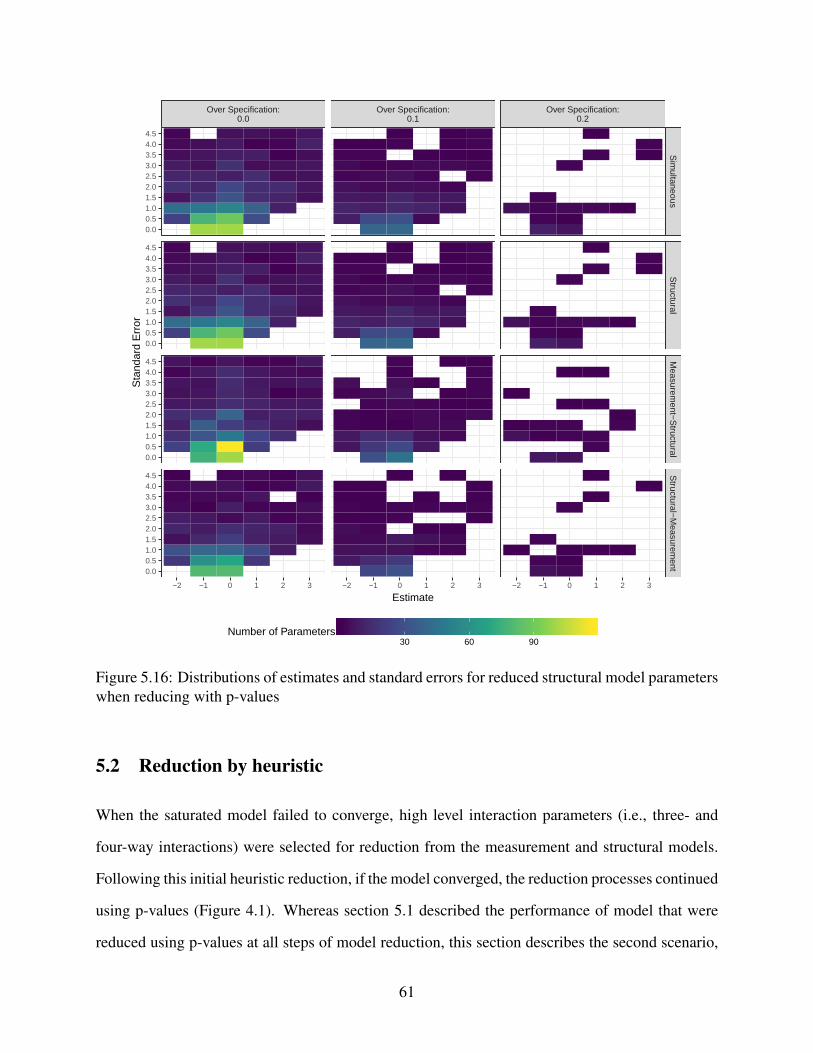
Over Specification:0.0
Over Specification:0.1
Over Specification:0.2
Sim
ultaneousS
tructuralM
easurement−
Structural
Structural−
Measurem
ent
−2 −1 0 1 2 3 −2 −1 0 1 2 3 −2 −1 0 1 2 3
0.00.51.01.52.02.53.03.54.04.5
0.00.51.01.52.02.53.03.54.04.5
0.00.51.01.52.02.53.03.54.04.5
0.00.51.01.52.02.53.03.54.04.5
Estimate
Sta
ndar
d E
rror
30 60 90Number of Parameters
Figure 5.16: Distributions of estimates and standard errors for reduced structural model parameterswhen reducing with p-values
5.2 Reduction by heuristic
When the saturated model failed to converge, high level interaction parameters (i.e., three- and
four-way interactions) were selected for reduction from the measurement and structural models.
Following this initial heuristic reduction, if the model converged, the reduction processes continued
using p-values (Figure 4.1). Whereas section 5.1 described the performance of model that were
reduced using p-values at all steps of model reduction, this section describes the second scenario,
61

where models were reduced with the heuristic first, and then p-values.
5.2.1 Convergence
Figure 5.17 shows the convergence rates for these reduction processes when the saturated model
failed to converge. Recall that measurement-structural and structural measurement reduction only
occurred if the measurement and structural reductions using the heuristic, respectively, converged.
When the Q-matrix is correctly specified, reduction of the structural model led to convergence the
majority of the time. Conversely, the removal of three- and four-way interactions in the measure-
ment model never led to convergence, unless the structural was being reduced simultaneously. The
measurement model was able to be reduced by p-values, but only after higher order interactions
had been reduced from the structural model.
62
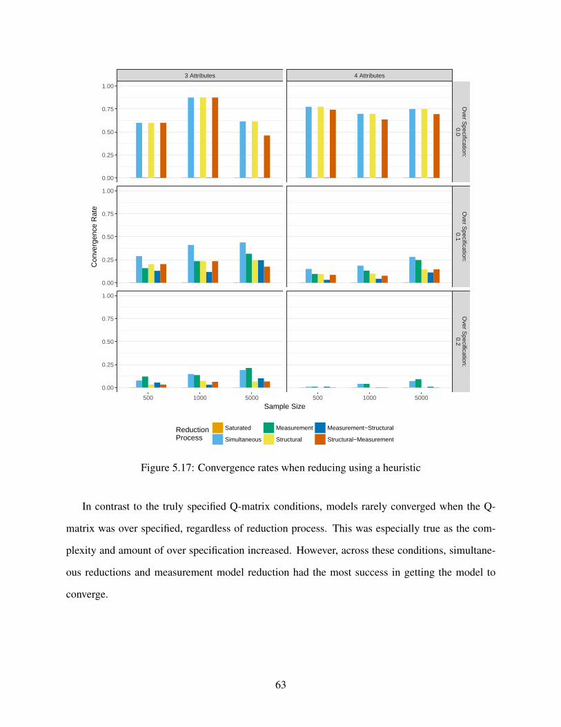
3 Attributes 4 Attributes
Over S
pecification:0.0
Over S
pecification:0.1
Over S
pecification:0.2
500 1000 5000 500 1000 5000
0.00
0.25
0.50
0.75
1.00
0.00
0.25
0.50
0.75
1.00
0.00
0.25
0.50
0.75
1.00
Sample Size
Con
verg
ence
Rat
e
ReductionProcess
Saturated
Simultaneous
Measurement
Structural
Measurement−Structural
Structural−Measurement
Figure 5.17: Convergence rates when reducing using a heuristic
In contrast to the truly specified Q-matrix conditions, models rarely converged when the Q-
matrix was over specified, regardless of reduction process. This was especially true as the com-
plexity and amount of over specification increased. However, across these conditions, simultane-
ous reductions and measurement model reduction had the most success in getting the model to
converge.
63
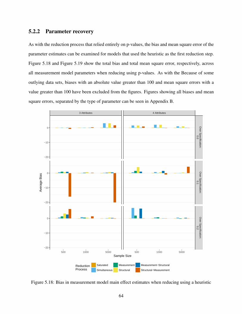
5.2.2 Parameter recovery
As with the reduction process that relied entirely on p-values, the bias and mean square error of the
parameter estimates can be examined for models that used the heuristic as the first reduction step.
Figure 5.18 and Figure 5.19 show the total bias and total mean square error, respectively, across
all measurement model parameters when reducing using p-values. As with the Because of some
outlying data sets, biases with an absolute value greater than 100 and mean square errors with a
value greater than 100 have been excluded from the figures. Figures showing all biases and mean
square errors, separated by the type of parameter can be seen in Appendix B.
3 Attributes 4 Attributes
Over S
pecification:0.0
Over S
pecification:0.1
Over S
pecification:0.2
500 1000 5000 500 1000 5000
−20
−10
0
−20
−10
0
−20
−10
0
Sample Size
Ave
rage
Bia
s
ReductionProcess
Saturated
Simultaneous
Measurement
Structural
Measurement−Structural
Structural−Measurement
Figure 5.18: Bias in measurement model main effect estimates when reducing using a heuristic
64
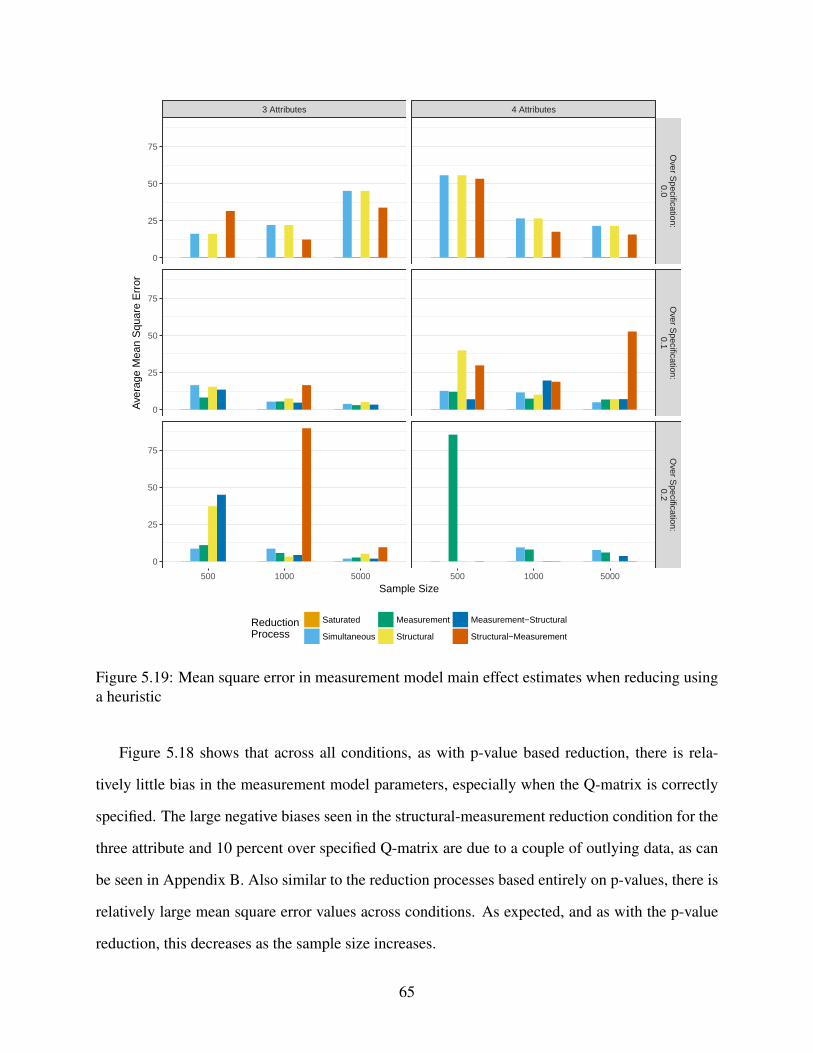
3 Attributes 4 Attributes
Over S
pecification:0.0
Over S
pecification:0.1
Over S
pecification:0.2
500 1000 5000 500 1000 5000
0
25
50
75
0
25
50
75
0
25
50
75
Sample Size
Ave
rage
Mea
n S
quar
e E
rror
ReductionProcess
Saturated
Simultaneous
Measurement
Structural
Measurement−Structural
Structural−Measurement
Figure 5.19: Mean square error in measurement model main effect estimates when reducing usinga heuristic
Figure 5.18 shows that across all conditions, as with p-value based reduction, there is rela-
tively little bias in the measurement model parameters, especially when the Q-matrix is correctly
specified. The large negative biases seen in the structural-measurement reduction condition for the
three attribute and 10 percent over specified Q-matrix are due to a couple of outlying data, as can
be seen in Appendix B. Also similar to the reduction processes based entirely on p-values, there is
relatively large mean square error values across conditions. As expected, and as with the p-value
reduction, this decreases as the sample size increases.
65
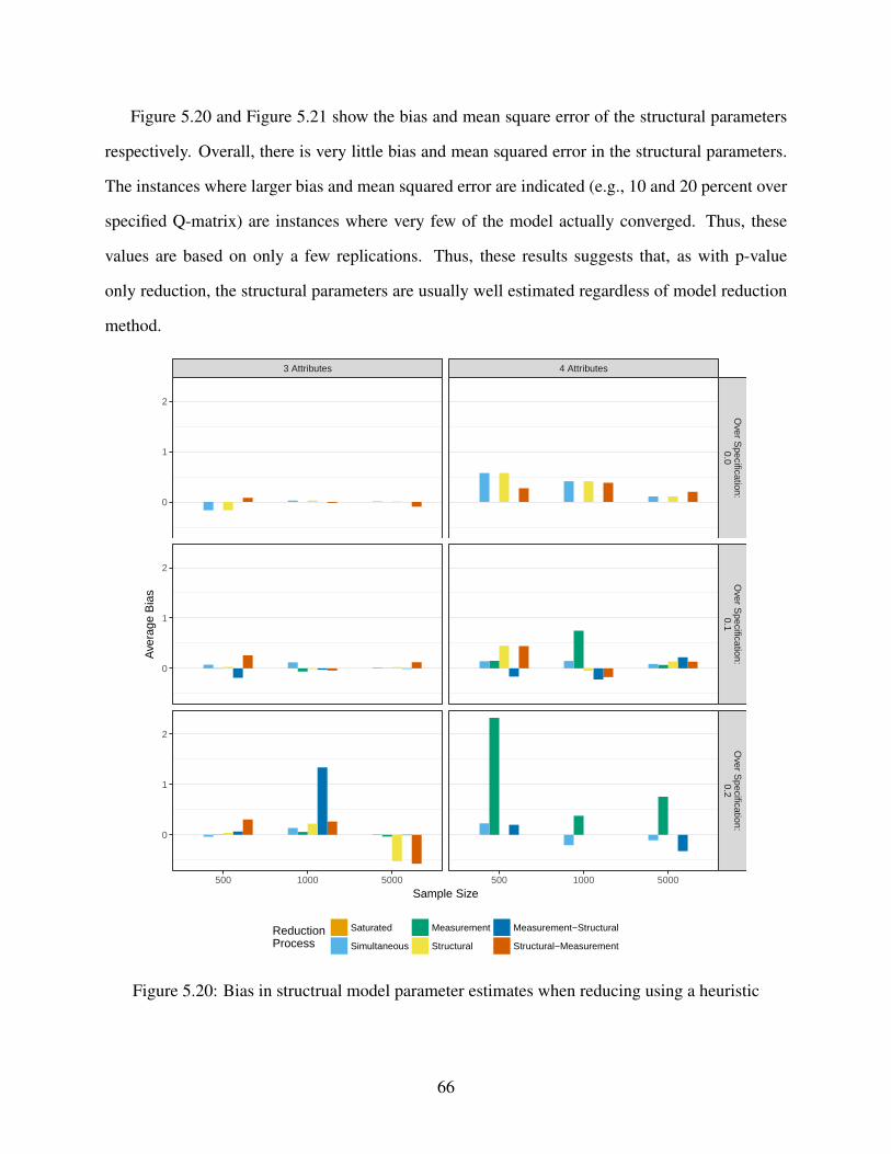
Figure 5.20 and Figure 5.21 show the bias and mean square error of the structural parameters
respectively. Overall, there is very little bias and mean squared error in the structural parameters.
The instances where larger bias and mean squared error are indicated (e.g., 10 and 20 percent over
specified Q-matrix) are instances where very few of the model actually converged. Thus, these
values are based on only a few replications. Thus, these results suggests that, as with p-value
only reduction, the structural parameters are usually well estimated regardless of model reduction
method.
3 Attributes 4 Attributes
Over S
pecification:0.0
Over S
pecification:0.1
Over S
pecification:0.2
500 1000 5000 500 1000 5000
0
1
2
0
1
2
0
1
2
Sample Size
Ave
rage
Bia
s
ReductionProcess
Saturated
Simultaneous
Measurement
Structural
Measurement−Structural
Structural−Measurement
Figure 5.20: Bias in structrual model parameter estimates when reducing using a heuristic
66
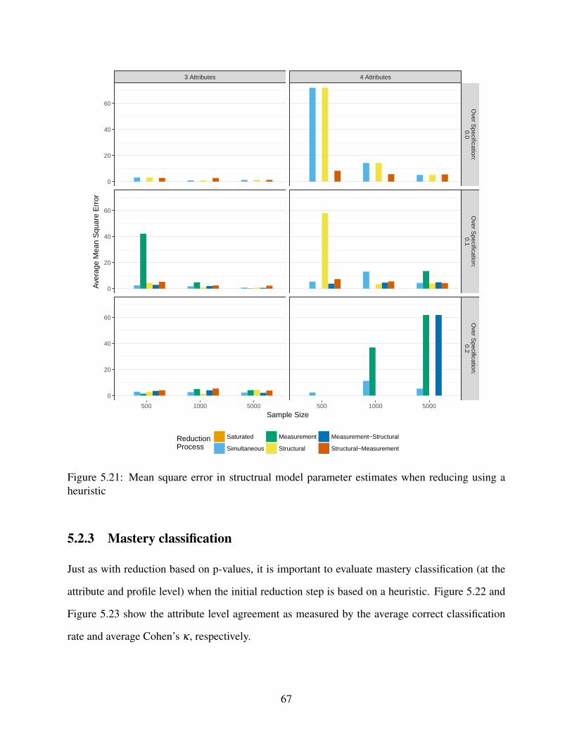
3 Attributes 4 Attributes
Over S
pecification:0.0
Over S
pecification:0.1
Over S
pecification:0.2
500 1000 5000 500 1000 5000
0
20
40
60
0
20
40
60
0
20
40
60
Sample Size
Ave
rage
Mea
n S
quar
e E
rror
ReductionProcess
Saturated
Simultaneous
Measurement
Structural
Measurement−Structural
Structural−Measurement
Figure 5.21: Mean square error in structrual model parameter estimates when reducing using aheuristic
5.2.3 Mastery classification
Just as with reduction based on p-values, it is important to evaluate mastery classification (at the
attribute and profile level) when the initial reduction step is based on a heuristic. Figure 5.22 and
Figure 5.23 show the attribute level agreement as measured by the average correct classification
rate and average Cohen’s κ , respectively.
67
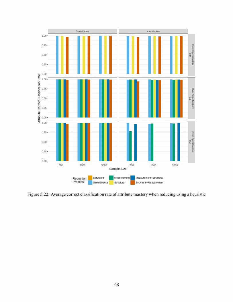
3 Attributes 4 Attributes
Over S
pecification:0.0
Over S
pecification:0.1
Over S
pecification:0.2
500 1000 5000 500 1000 5000
0.00
0.25
0.50
0.75
1.00
0.00
0.25
0.50
0.75
1.00
0.00
0.25
0.50
0.75
1.00
Sample Size
Attr
ibut
e C
orre
ct C
lass
ifica
tion
Rat
e
ReductionProcess
Saturated
Simultaneous
Measurement
Structural
Measurement−Structural
Structural−Measurement
Figure 5.22: Average correct classification rate of attribute mastery when reducing using a heuristic
68
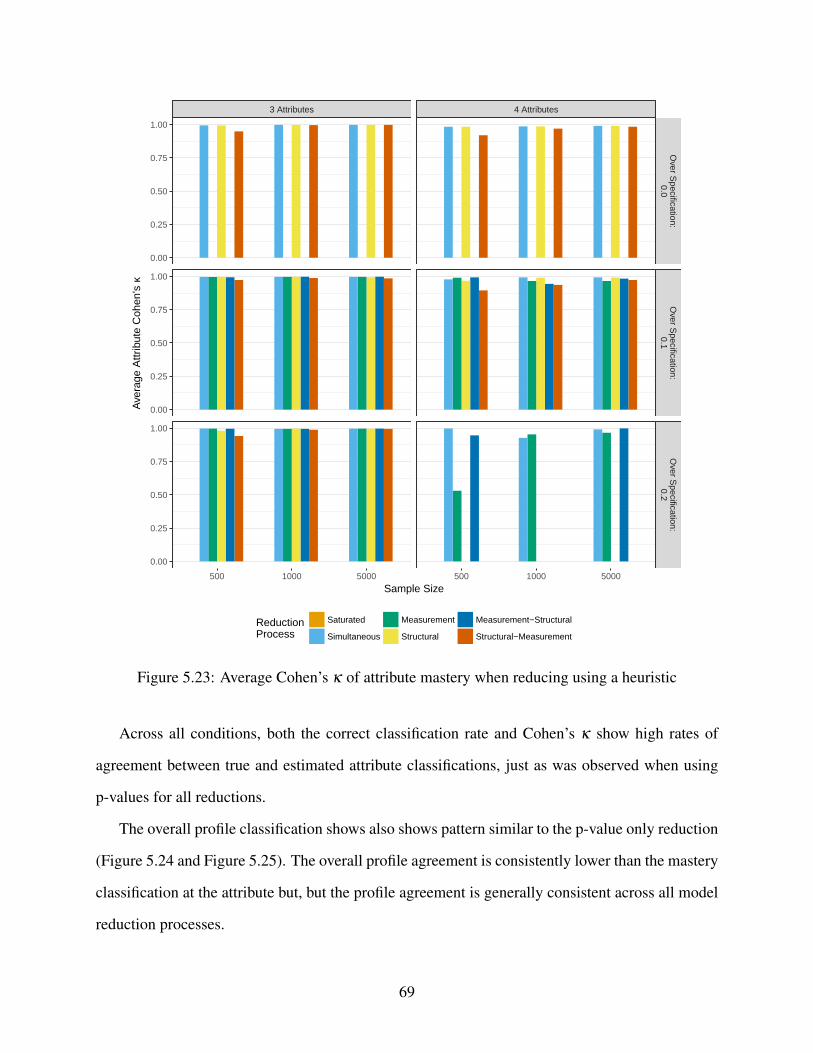
3 Attributes 4 Attributes
Over S
pecification:0.0
Over S
pecification:0.1
Over S
pecification:0.2
500 1000 5000 500 1000 5000
0.00
0.25
0.50
0.75
1.00
0.00
0.25
0.50
0.75
1.00
0.00
0.25
0.50
0.75
1.00
Sample Size
Ave
rage
Attr
ibut
e C
ohen
's κ
ReductionProcess
Saturated
Simultaneous
Measurement
Structural
Measurement−Structural
Structural−Measurement
Figure 5.23: Average Cohen’s κ of attribute mastery when reducing using a heuristic
Across all conditions, both the correct classification rate and Cohen’s κ show high rates of
agreement between true and estimated attribute classifications, just as was observed when using
p-values for all reductions.
The overall profile classification shows also shows pattern similar to the p-value only reduction
(Figure 5.24 and Figure 5.25). The overall profile agreement is consistently lower than the mastery
classification at the attribute but, but the profile agreement is generally consistent across all model
reduction processes.
69
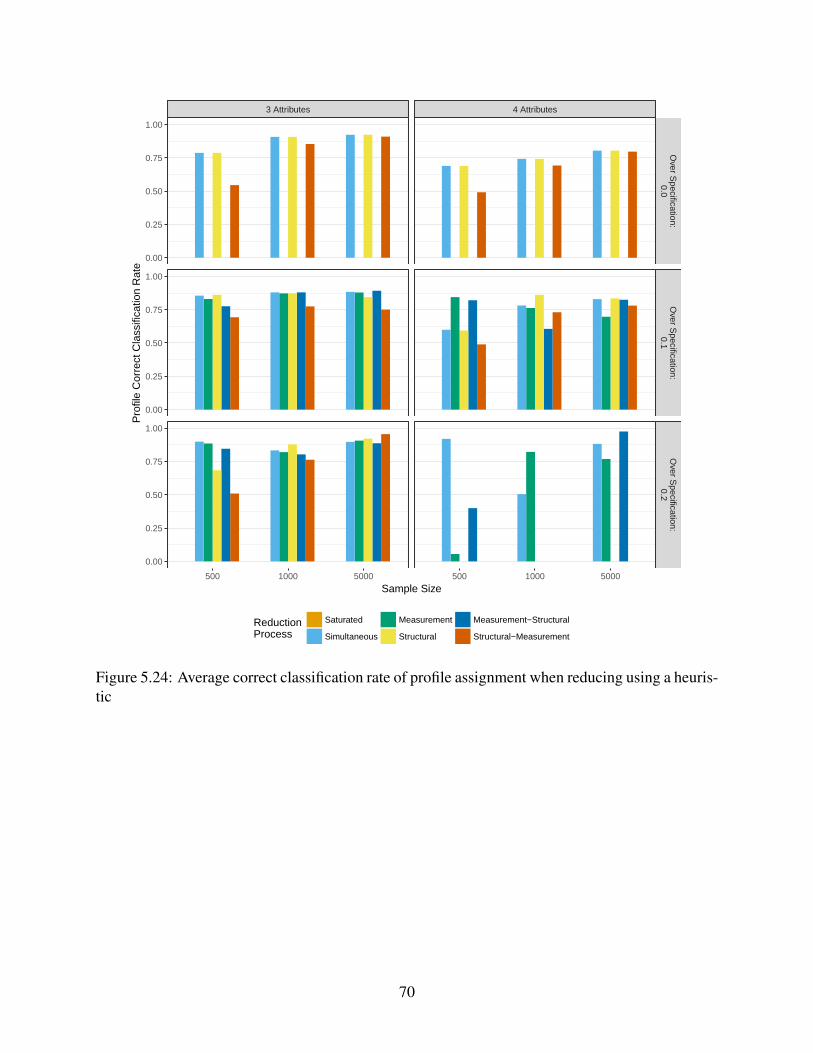
3 Attributes 4 Attributes
Over S
pecification:0.0
Over S
pecification:0.1
Over S
pecification:0.2
500 1000 5000 500 1000 5000
0.00
0.25
0.50
0.75
1.00
0.00
0.25
0.50
0.75
1.00
0.00
0.25
0.50
0.75
1.00
Sample Size
Pro
file
Cor
rect
Cla
ssifi
catio
n R
ate
ReductionProcess
Saturated
Simultaneous
Measurement
Structural
Measurement−Structural
Structural−Measurement
Figure 5.24: Average correct classification rate of profile assignment when reducing using a heuris-tic
70
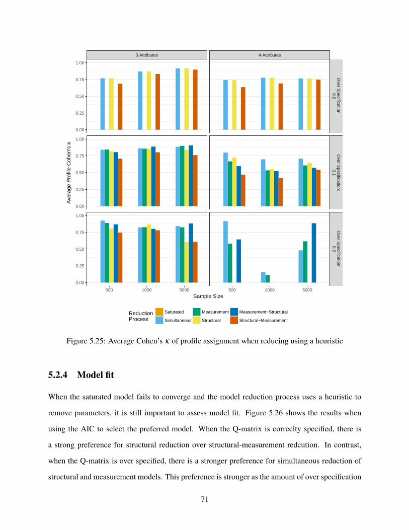
3 Attributes 4 Attributes
Over S
pecification:0.0
Over S
pecification:0.1
Over S
pecification:0.2
500 1000 5000 500 1000 5000
0.00
0.25
0.50
0.75
1.00
0.00
0.25
0.50
0.75
1.00
0.00
0.25
0.50
0.75
1.00
Sample Size
Ave
rage
Pro
file
Coh
en's
κ
ReductionProcess
Saturated
Simultaneous
Measurement
Structural
Measurement−Structural
Structural−Measurement
Figure 5.25: Average Cohen’s κ of profile assignment when reducing using a heuristic
5.2.4 Model fit
When the saturated model fails to converge and the model reduction process uses a heuristic to
remove parameters, it is still important to assess model fit. Figure 5.26 shows the results when
using the AIC to select the preferred model. When the Q-matrix is correclty specified, there is
a strong preference for structural reduction over structural-measurement redcution. In contrast,
when the Q-matrix is over specified, there is a stronger preference for simultaneous reduction of
structural and measurement models. This preference is stronger as the amount of over specification
71
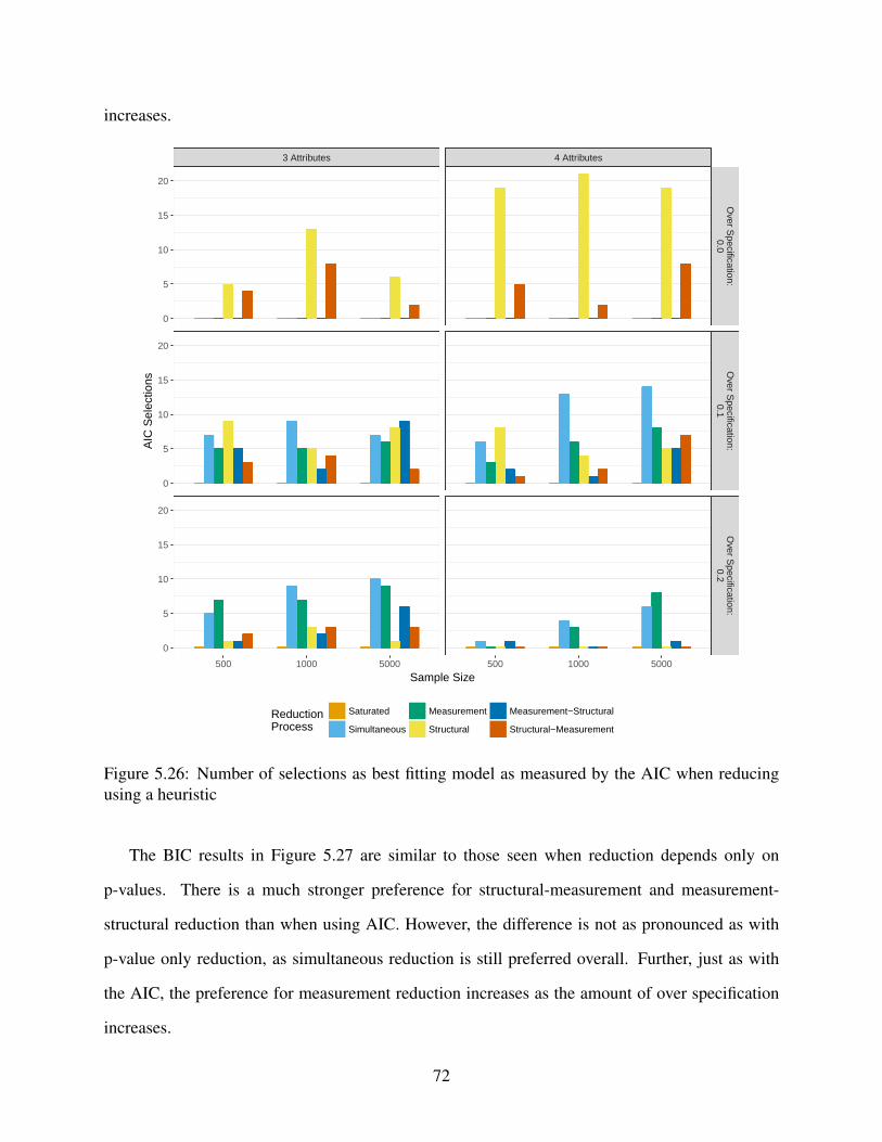
increases.
3 Attributes 4 AttributesO
ver Specification:0.0
Over S
pecification:0.1
Over S
pecification:0.2
500 1000 5000 500 1000 5000
0
5
10
15
20
0
5
10
15
20
0
5
10
15
20
Sample Size
AIC
Sel
ectio
ns
ReductionProcess
Saturated
Simultaneous
Measurement
Structural
Measurement−Structural
Structural−Measurement
Figure 5.26: Number of selections as best fitting model as measured by the AIC when reducingusing a heuristic
The BIC results in Figure 5.27 are similar to those seen when reduction depends only on
p-values. There is a much stronger preference for structural-measurement and measurement-
structural reduction than when using AIC. However, the difference is not as pronounced as with
p-value only reduction, as simultaneous reduction is still preferred overall. Further, just as with
the AIC, the preference for measurement reduction increases as the amount of over specification
increases.
72
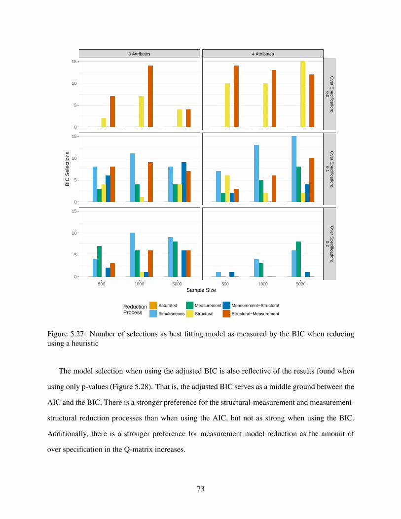
3 Attributes 4 Attributes
Over S
pecification:0.0
Over S
pecification:0.1
Over S
pecification:0.2
500 1000 5000 500 1000 5000
0
5
10
15
0
5
10
15
0
5
10
15
Sample Size
BIC
Sel
ectio
ns
ReductionProcess
Saturated
Simultaneous
Measurement
Structural
Measurement−Structural
Structural−Measurement
Figure 5.27: Number of selections as best fitting model as measured by the BIC when reducingusing a heuristic
The model selection when using the adjusted BIC is also reflective of the results found when
using only p-values (Figure 5.28). That is, the adjusted BIC serves as a middle ground between the
AIC and the BIC. There is a stronger preference for the structural-measurement and measurement-
structural reduction processes than when using the AIC, but not as strong when using the BIC.
Additionally, there is a stronger preference for measurement model reduction as the amount of
over specification in the Q-matrix increases.
73

3 Attributes 4 Attributes
Over S
pecification:0.0
Over S
pecification:0.1
Over S
pecification:0.2
500 1000 5000 500 1000 5000
0
5
10
15
0
5
10
15
0
5
10
15
Sample Size
Adj
uste
d B
IC S
elec
tions
ReductionProcess
Saturated
Simultaneous
Measurement
Structural
Measurement−Structural
Structural−Measurement
Figure 5.28: Number of selections as best fitting model as measured by the adjusted BIC whenreducing using a heuristic
5.2.5 Description of reduced parameters
Finally, the performance of the different processes in terms of correctly specifying the parameters
to be included can be examined. Figure 5.29 shows the proportion of time the measurement model
was correctly reduced, and Figure 5.30 shows the proportion of correct reductions for the structural
model.
74

3 Attributes 4 Attributes
Over S
pecification:0.0
Over S
pecification:0.1
Over S
pecification:0.2
500 1000 5000 500 1000 5000
0.00
0.25
0.50
0.75
1.00
0.00
0.25
0.50
0.75
1.00
0.00
0.25
0.50
0.75
1.00
Sample Size
Pro
post
ion
of C
orre
ct R
educ
tions
ReductionProcess
Saturated
Simultaneous
Measurement
Structural
Measurement−Structural
Structural−Measurement
Figure 5.29: Proportion of correct measurement model reductions when reducing with a heuristic
75
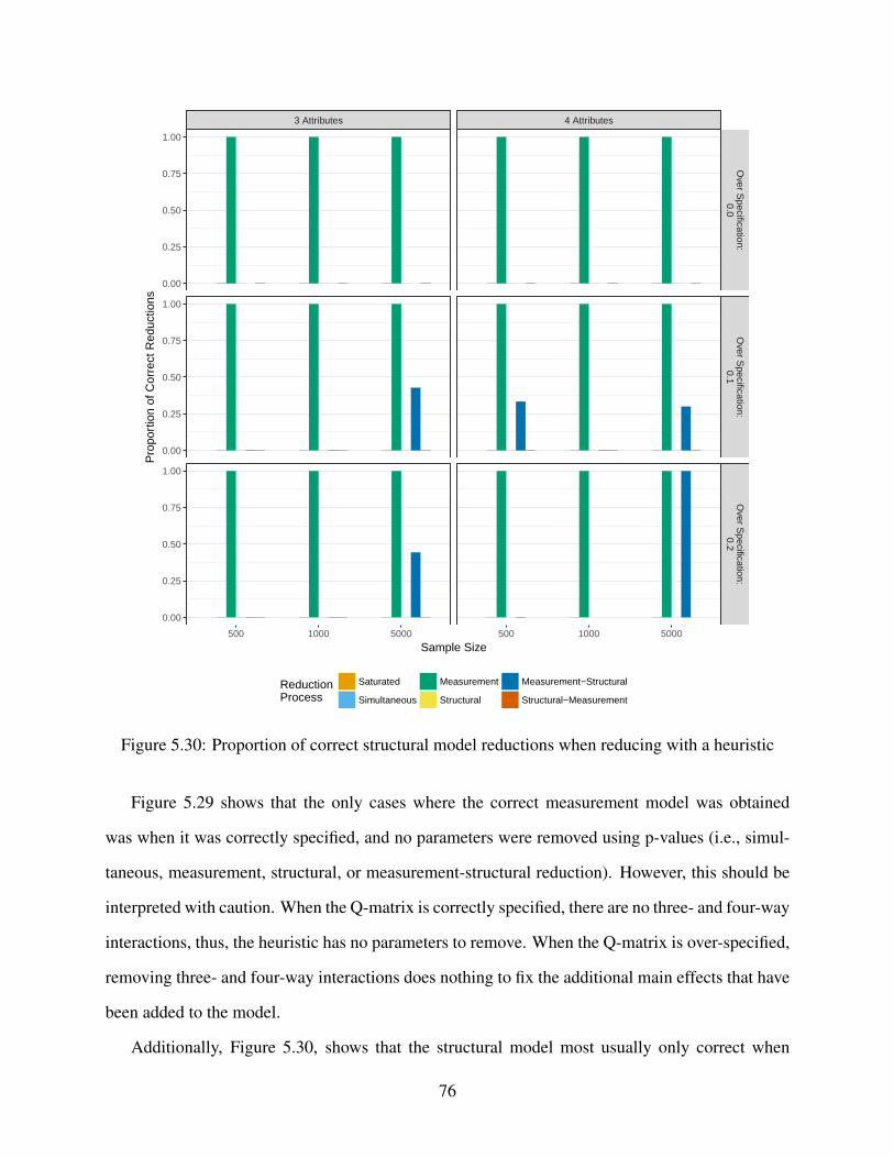
3 Attributes 4 Attributes
Over S
pecification:0.0
Over S
pecification:0.1
Over S
pecification:0.2
500 1000 5000 500 1000 5000
0.00
0.25
0.50
0.75
1.00
0.00
0.25
0.50
0.75
1.00
0.00
0.25
0.50
0.75
1.00
Sample Size
Pro
port
ion
of C
orre
ct R
educ
tions
ReductionProcess
Saturated
Simultaneous
Measurement
Structural
Measurement−Structural
Structural−Measurement
Figure 5.30: Proportion of correct structural model reductions when reducing with a heuristic
Figure 5.29 shows that the only cases where the correct measurement model was obtained
was when it was correctly specified, and no parameters were removed using p-values (i.e., simul-
taneous, measurement, structural, or measurement-structural reduction). However, this should be
interpreted with caution. When the Q-matrix is correctly specified, there are no three- and four-way
interactions, thus, the heuristic has no parameters to remove. When the Q-matrix is over-specified,
removing three- and four-way interactions does nothing to fix the additional main effects that have
been added to the model.
Additionally, Figure 5.30, shows that the structural model most usually only correct when
76

only the measurement model was reduced. This is because the data was always generated with a
fully saturated structural model. Thus, any removal of parameters (including three- and four-way
interactions) results in an incorrect final model.
77
Chapter 6
Conclusions
The present study utilizes Monte Carlo simulation to evaluate the performance of various model
reduction processes for diagnostic classification models. There are two components of DCMs
that can be reduced during the estimation process: the measurement model and the structural
model. The measurement model governs how items related to the attributes, and the structural
model controls the base rate probabilities of inclusion in each class. In this study, the relative
strengths and weaknesses of reducing each model, and in which order was examined. Specifically,
convergence rates, the bias and mean square error of the parameter estimates, and the attribute and
profile mastery classifications were used to evaluate the processes.
Parameters were chosen for reduction based on their p-value. If after estimation of the prior
model in the reduction process the parameter was non-significant (i.e., p-value greater than .05), it
was removed from the model in the next iteration. In addition, parameters could also be reduced
using a heuristic if the saturated model failed to converge. In practice, practitioners are unlikely
to stop if the saturated model fails to converge, and instead remove parameters in an effort to
achieve a converged model (e.g., Bradshaw et al., 2014). Thus, if the saturated model failed to
converge, three- and four-way interaction terms were removed from the measurement and/or satu-
rated models for the reduction. Following the initial heuristic decision, subsequent reductions were
performed based on p-values of converged models. These two processes (p-value only reduction
and heuristic and p-value reduction) were analyzed separately to evaluate possible differences in
reduction preference.
Overall, the results suggest that all model reduction processes provide reasonably unbiased
estimates of measurement model and structural model parameters, and mean square error decreased
78
as the sample size increased. Additionally, all reduction processes showed high levels of agreement
between the true and estimated attribute mastery of the respondents. This was especially at the
attribute level as compared to the profile level, but showed a consistent pattern across both p-value
based and heuristic based reduction.
However, a key difference found in this study was the convergence rates of different model
reduction processes, and how those were affected by the initial convergence of the saturated model.
When the saturated model converged, reducing the measurement model first was most likely to
lead to a converged model, especially if the Q-matrix was over specified. In contrast, when the
saturated model failed to converge, reducing the structural model was far more likely to lead to
model convergence. This was most pronounced in the correctly specified Q-matrix conditions.
Regardless of whether or not the saturated model converged, model reductions were unlikely to
result in a converged solution when the Q-matrix was over specified. The overall low rate over
convergence for the over specified Q-matrices, across all conditions, indicates that the model is
highly unlikely to converge if the Q-matrix has even low rates of over specification.
Additionally, the model fit results suggest other differences. When the saturated model success-
fully converged, that was most often the preferred model. Obviously when the saturated model fails
to converge, this is not an option. In this scenario, structural reduction was the preferred method
of model reduction. It is possible that this finding for the heuristic reduction is an artifact of the
structural reduction converging the most frequently. However, structural reduction was also the
second most preferred reduction process when reducing with p-values. Together, this suggests that
reduction of the structural model is less likely to negatively impact model fit on average.
Taken in totality, the results of this study suggest that the path of model reduction should be
determined by the convergence of the saturated model. Should the saturated model converge, then
the measurement model should be reduced first in order to create a more parsimonious model,
while still maintaining a converged solution. On the other hand, if the saturated model fails to
converge, reducing the structural model is most likely to provide a converged solution to evaluate.
If this too fails to converge, then the most likely scenario is that the Q-matrix has been misspecified,
79
and should be revised with input from content area experts, just as in the process for developing
the Q-matrix (Bradshaw, 2017).
6.1 Limitations and future directions
There are several limitations of this study that deserve additional investigation in future work. First,
reduction of converged models was based on p-values. The reliance on p-values is problematic for
several reasons. For example, p-values do not give direct inferences about the parameter values,
and they are unable to provide information about the actual size of the effect (see Wasserstein &
Lazar, 2016 for a more complete summary). However, because of the .05 cutoff used to identify
non-significant parameters for reduction, there is likely a non-negligible amount of Type I error.
Instead, it would likely be better to use a Bayesian estimation, where credible intervals could
be formed around the parameter estimates, and reduced based on the proportion of the posterior
distribution that is below a predefined cutoff of practical significance. Improvements in available
software for estimating DCMs is likely necessary in order for this to be a viable path forward.
Secondly, the random generation of structural parameters resulted in respondents being un-
evenly placed into classes. Although this may be more reflective of reality, where some classes are
less likely than others (for example Figure 3.2), it also likely contributed to convergence problems.
Thus, future research may benefit from having a fixed structural model, or least utilizing some
mechanism of ensuring that respondents are present in all classes. As an example, it would be
relatively straight forward when generating the structural parameters to keep regenerating param-
eters until a set is generated that results in all classes having a base rate probability above a given
threshold.
Related to the issues of under represented classes, part of the model reduction process could
involve removing classes that have a low number of respondents assigned to them (e.g., Templin
& Bradshaw, 2014a). The implementation of this process would present several challenges. For
instance, without theoretical support for why a given profile may or should not exist in the popula-
tion, there is no straight forward method for assessing whether or not a profile should be removed
80
from the model. In other words, there is a problem in deciding how large a class must be in order
for it to be retained. The base rate probabilities could be used, but then a determination must be
made about what percentage constitutes a non-significant proportion of the population. Despite
these complications, this remains an important area of future research.
Finally, it should be noted that the model selection process should not merely be an exercise
in finding a path to convergence. The findings of this study are largely driven by the convergence
rates of various model reduction processes. Although this is an important outcome measure, a
model should not be selected for use due solely to the fact that it was able to converge. Rather,
additional and more accurate measures of model fit are necessary to support the use of a model.
Mplus provides χ2 statistics for univariate and bivariate sets of items; however, these are unable
to sufficiently assess model fit due to the violations of the asymptotic assumptions of the distribu-
tions. Instead, model fit may be better assessed through posterior predictive model checks from a
Bayesian estimation (e.g., Gelman & Hill, 2006; Gelman et al., 2014). In this way, the practitioner
can evaluate the overall fit of the model to data, not just compare between models that were able
to successfully converge.
Despite these limitations, this study provides the first empirical evaluation of model reduction
processes in DCMs. As the operational use of these models continues to grow, continued research
into the practical applications of DCMs will need to keep pace. This study not only demonstrates
a framework for future research into the application of DCMs, but also provides guidance to re-
searchers and practitioners as to how best to proceed with model estimation.
81
References
Agresti, A. (2012). Categorical Data Analysis (3rd ed.). New York, NY: John Wiley & Sons.
Akaike, H. (1974). A new look at the statistical model identification. IEEE Transactions on
Automatic Control, 19(6), 716–723. https://doi.org/10.1109/TAC.1974.1100705
Allaire, J., Cheng, J., Xie, Y., McPherson, J., Chang, W., Allen, J., . . . Arslan, R. (2017). rmark-
down: Dynamic documents for R. Retrieved from http://rmarkdown.rstudio.com
Almond, R. G., Mislevy, R. J., Steinberg, L. S., Yan, D., & Williamson, D. M. (2015). Bayesian
Networks in Educational Assessment (1st ed.). New York, NY: Springer.
Amazon Web Services. (2018). Amazon Elastic Compute Cloud (EC2). Retrieved from https:
//aws.amazon.com/ec2/
Ayala, R. J. de. (2009). The Theory and Practice of Item Response Theory. New York, NY:
Guilford Press.
Bradshaw, L. (2017). Diagnostic Classification Models. In A. A. Rupp & J. Leighton (Eds.), The
Handbook of Cognition and Assessment: Frameworks, Methodologies, and Applications (1st
ed., pp. 297–327). New York, NY: John Wiley & Sons.
Bradshaw, L., & Templin, J. (2014). Combining item response theory and diagnostic classification
models: A psychometric model for scaling ability and diagnosing misconceptions. Psychome-
trika, 79(3), 403–425. https://doi.org/10.1007/s11336-013-9350-4
Bradshaw, L., Izsák, A., Templin, J., & Jacobson, E. (2014). Diagnosing teachers’ understand-
ings of rational numbers: Building a multidimensional test within the diagnostic classification
framework. Educational Measurement: Issues and Practice, 33(1), 2–14.
Brown, T. A. (2006). Confirmatory Factor Analysis for Applied Research. New York, NY: Guil-
ford.
Browne, M., Rockloff, M., & Rawat, V. (2016). An SEM algorithm for scale reduction incorporat-
82
ing evaluation of multiple psychometric criteria. Sociological Methods & Research, (Advance
online publication). https://doi.org/10.1177/0049124116661580
Burkholder, G. J., & Harlow, L. L. (2003). An illustration of longitudinal cross-lagged design
for larger structual equation models. Structural Equation Modeling, 10(3), 465–486. https:
//doi.org/10.1207/S15328007SEM1003_8
Chen, Y., Liu, J., Xu, G., & Ying, Z. (2015). Statistical analysis of Q-matrix based diagnostic
classification models. Journal of the American Statistical Association, 110(510), 850–866.
https://doi.org/10.1080/01621459.2014.934827
Chinn, S. (2000). A simple method for converting an odds ratio to effect size for use in meta-
analysis. Statistics in Medicine, 19, 3127–3131.
Cizek, G. J. (2006). Standard Setting. In S. M. Downing & T. M. Haladyna (Eds.), Handbook of
Test Development. Mahwah, NJ: Taylor & Francis.
Cohen, J. (1960). A coefficient of agreement for nominal scales. Educational and Psychological
Measurement, 20(1), 37–46.
Cohen, J. (1968). Weighted kappa: Nominal scale agreement with provision for scaled disagree-
ment or partial credit. Psychological Bulletin, 70(4), 213–220.
de la Torre, J. (2008). An empirically based method of Q-matrix validation for the DINA model:
Development and applications. Journal of Educational Measurement, 45(4), 343–362. https:
//doi.org/10.1111/j.1745-3984.2008.00069.x
de la Torre, J., & Douglas, J. A. (2004). Higher-order latent trait models for cognitive diagnosis.
Psychometrika, 69(3), 333–353. https://doi.org/10.1007/BF02295640
de la Torre, J., Ark, L. A. van der, & Rossi, G. (2015). Analysis of clinical data from cognitive
diagnosis modeling framework. Measurement and Evaluation in Counseling and Development,
0748175615569110. https://doi.org/10.1177/0748175615569110
DeCarlo, L. T. (2011). On the analysis of fraction bubtraction data: The DINA model, classifi-
cation, latent class sizes, and the Q-matrix. Applied Psychological Measurement, 35(1), 8–26.
83
https://doi.org/10.1177/0146621610377081
DeVellis, R. F. (2006). Classical test theory. Medical Care, 44(11), S50–S59. Retrieved from
http://journals.lww.com/lww-medicalcare/Fulltext/2006/11001/Classical_Test_
Theory.11.aspx
DiBello, L. V., Stout, W. F., & Roussos, L. (1995). Unified cognitive psychometric assessment
likelihood-based classification techniques. In P. D. Nichols, S. F. Chipman, & R. L. Brennan
(Eds.), Cognitively Diagnostic Assessment (pp. 361–390). Hillsdale, NJ: Erlbaum.
Feinberg, R. A., & Rubright, J. D. (2016). Conducting simulation studies in psychometrics. Ed-
ucational Measurement: Issues and Practice, 35(2), 36–49. https://doi.org/10.1111/
emip.12111
Feinberg, R. A., & Wainer, H. (2014). When can we improve subscores by making them shorter?:
The case against sbuscores with overlapping items. Educational Measurement: Issues and
Practice, 33(3), 47–54.
Fukuhara, H., & Kamata, A. (2011). A bifactor multidimensional item response theory model for
differential item functioning analysis on testlet-based items. Applied Psychological Measure-
ment, 35(8), 604–622. https://doi.org/10.1177/0146621611428447
Gelman, A., & Hill, J. (2006). Data Analysis Using Regression and Multilevel/Hierarchical Mod-
els (1st ed.). Cambridge, England: Cambridge University Press.
Gelman, A., Carlin, J. B., Stern, H. S., Dunson, D. B., Vehtari, A., & Rubin, D. B. (2014). Bayesian
Data Analysis (3rd ed.). Boca Raton, FL: CRC Press.
Haertel, E. H. (1989). Using restricted latent class models to map the skill structure of achievement
items. Journal of Educational Measurement, 26(4), 301–321. Retrieved from http://www.
jstor.org/stable/1434756
Hallquist, M., & Wiley, J. (2018). MplusAutomation: An r package for facilitating large-scale
latent variable analyses in mplus. Retrieved from https://CRAN.R-project.org/package=
MplusAutomation
Halonen, J., Harris, C. M., Pastor, D. A., Abrahamson, C. E., & Huffman, C. J. (2005). Assessing
84
general education outcomes in introductory psychology. In D. S. Dunn & S. Chew (Eds.), Best
Practices in Teaching Introduction to Psychology (pp. 195–210). Mahwah, NJ: Erlbaum.
Hambleton, R. (2006). Setting Performance Standards. In Educational Measurement (4th ed., pp.
433–470). Rowman & Littelfield.
Hartz, S. M. (2002). A Bayesian framework for the unified model for assessing cognitive abilities:
Blending theory with practicality (Unpublished doctoral dissertation). University of Illinois at
Urbana-Champaign, Urbana-Champaign, IL.
Harwell, M., Stone, C. A., Hsu, T.-C., & Kirisci, L. (1996). Monte Carlo studies in item response
theory. Applied Psychological Measurement, 20(2), 101–125.
Henry, L., & Wickham, H. (2017). Purrr: Functional programming tools. Retrieved from https:
//CRAN.R-project.org/package=purrr
Henry, L., & Wickham, H. (2018). Tidyselect: Select from a set of strings. Retrieved from https:
//CRAN.R-project.org/package=tidyselect
Henson, R. A., Templin, J. L., & Willse, J. T. (2008). Defining a family of cognitive diagnosis
models using log-linear models with latent variables. Psychometrika, 74(2), 191. https:
//doi.org/10.1007/s11336-008-9089-5
Henson, R., & Douglas, J. (2005). Test construction for cognitive diagnosis. Applied Psychological
Measurement, 29(4), 262–277. https://doi.org/10.1177/0146621604272623
Henson, R., & Templin, J. (2005). Extending cognitive diagnosis models to evaluate the validity
of DSM criteria for the diagnosis of pathological gambling. In. Las Vegas, NV.
Hester, J. (2017). Glue: Interpreted string literals. Retrieved from https://CRAN.R-project.
org/package=glue
Johnson, P. E. (2016). PortableParallelSeeds: Allow replication of simulations on parallel and se-
rial computers. Retrieved from https://CRAN.R-project.org/package=portableParallelSeeds
Junker, B. W., & Sijtsma, K. (2001). Cognitive assessment models with few assumptions, and
connections with nonparametric item response theory. Applied Psychological Measurement,
85
25(3), 258–272. https://doi.org/10.1177/01466210122032064
Jurich, D. P., & Bradshaw, L. (2013). An illustration of diagnostic classification modeling in
student learning outcomes assessment. International Journal of Testing, 14(1), 49–72.
Kaplan, D. (2009). Structural Equation Modeling: Foundations and Extensions (2nd ed.). Thou-
sand Oaks, CA: Sage.
Kingston, N. M., & McKinley, R. L. (1988). Assessing the structure of the GRF General Test using
confirmatory multidimensional item response theory. In Symposium: Item response theory
meets multidimensional tests. New Orleans, LA.
Kline, R. B. (2002). Principles and Practice of Structural Equation Modeling (2nd ed.). New
York, NY: Guilford.
Kunina-Habenicht, O., Rupp, A. A., & Wilhelm, O. (2012). The impact of model misspecifi-
cation on parameter estimation and item-fit assessment in log-linear diagnostic classification
models. Journal of Educational Measurement, 49(1), 59–81. https://doi.org/10.1111/j.
1745-3984.2011.00160.x
McKinley, R. L., & Kingston, N. M. (1988). Confirmatory analysis of test structure using multidi-
mensional IRT. In. New Orleans, LA.
McWhite, C. D., & Wilke, C. O. (2018). Colorblindr: Simulate colorblindness in r figures. Re-
trieved from https://github.com/clauswilke/colorblindr
Millon, T., Millon, C., Davis, R., & Grossman, S. (2009). MCMI-III Manual (4th ed.). Minneapo-
lis, MN: Pearson.
Muthén, L. K., & Muthén, B. O. (1998). Mplus User’s Guide (7th ed.). Los Angeles, CA: Muthén
& Muthén.
Müller, K., & Wickham, H. (2018). Tibble: Simple data frames. Retrieved from https://CRAN.
R-project.org/package=tibble
Netlify. (2018). Netlify. Retrieved from https://www.netlify.com/
Pandoc. (2017). Retrieved from https://pandoc.org/
Pedersen, T. L. (2016). Ggforce: Accelerating ’ggplot2’. Retrieved from https://github.com/
86
thomasp85/ggforce
Perry, J. L., Nicholls, A. R., Clough, P. J., & Crust, L. (2015). Assessing model fit: Caveats and
recommendations for confirmatory factor analysis and exploratory structural equation model-
ing. Measurement in Physical Education and Exercise Science, 19(1), 12–21.
Preston-Werner, T. (2018). Jekyll. Retrieved from https://jekyllrb.com/
R Core Team. (2017). R: A language and environment for statistical computing. Vienna, Austria:
R Foundation for Statistical Computing. Retrieved from https://www.R-project.org/
Reckase, M. D. (1997). The past and future of multidimensional item response theory. Applied
Psychological Measurement, 21(1), 25–36. https://doi.org/10.1177/0146621697211002
Reckase, M. D. (2009). Multidimensional Item Response Theory. New York, NY: Springer-Verlag.
Rojas, G., de la Torre, J., & Olea, J. (2012). Choosing between general and specific cognitive
diagnosis models when the sample size is small. In. Vancouver, British Columbia, Canada.
RStudio. (2018). RStudio. Retrieved from https://www.rstudio.com/products/rstudio/
Rubinstein, R. Y., & Kroese, D. P. (2017). Simulation and the Monte Carlo Method (3rd ed.).
Hoboken, NJ: Wiley.
Rupp, A. A., & Templin, J. (2008a). The effects of Q-matrix misspecification on parameter es-
timates and classification accuracy in the DINA model. Educational and Psychological Mea-
surement, 68(1), 78–96. https://doi.org/10.1177/0013164407301545
Rupp, A. A., & Templin, J. L. (2008b). Unique characteristics of diagnostic classification mod-
els: A comprehensive review of the current state-of-the-art. Measurement: Interdisciplinary
Research & Perspective, 6(4), 219–262. https://doi.org/10.1080/15366360802490866
Rupp, A. A., & Wilhelm, O. (2012). Files for Mplus input file generation. College Park, MD. Re-
trieved from http://www.education.umd.edu/EDMS/fac/Rupp/R%20Files%20for%20Mplus%
20Input%20File%20Generation.zip
Rupp, A. A., Templin, J., & Henson, R. A. (2010). Diagnostic Measurement: Theory, Meth-
ods, and Applications (1st ed.). New York, NY: Guilford Press. Retrieved from https://www.
87
guilford.com/books/Diagnostic-Measurement/Rupp-Templin-Henson/9781606235270
Schwarz, G. (1978). Estimating the dimension of a model. The Annals of Statistics, 6(2), 461–464.
https://doi.org/10.1214/aos/1176344136
Sclove, S. L. (1987). Application of model-selection criteria to some problems in multivariate
analysis. Psychometrika, 52(3), 333–343. https://doi.org/10.1007/BF02294360
Sinharay, S. (2010). When can subscores be expected to have added value? Results from opera-
tional and simulated data (No. RR-10-16). Princeton, NJ: Educational Testing Service.
Sinharay, S., Haberman, S. J., & Wainer, H. (2011). Do adjusted subscores lack validity? Don’t
blame the messenger. Educational and Psychological Measurement, 71(5), 789–797. https:
//doi.org/10.1177/0013164410391782
Skrondal, A., & Rabe-Hesketh, S. (2004). Generalized Latent Variable Modeling: Multilevel,
Longitudinal, and Structural Equation Models. New York, NY: Chapman & Hall/CRC.
Spinu, V., Grolemund, G., & Wickham, H. (2018). Lubridate: Make dealing with dates a little
easier. Retrieved from https://CRAN.R-project.org/package=lubridate
Stroup, W. W. (2012). Generalized Linear Mixed Models: Modern Concepts, Methods and Appli-
cations. New York, NY: Chapman & Hall/CRC.
Tatsuoka, K. K. (1983). Rule space: An approach for dealing with misconceptions based on item
response theory. Journal of Educational Measurement, 20, 345–354.
Tatsuoka, K. K. (1990). Toward an Integration of Item-Response Theory and Cognitive Error Di-
agnosis. In N. Frederiksen, R. Glaser, A. Lesgold, & M. Shafto (Eds.), Diagnostic Monitoring
of Skill and Knowledge Acquisition (pp. 453–488). Hillsdale, NJ: Erlbaum.
Templin, J. (2010). Classification model based standard setting methods. In. Denver, CO.
Templin, J. L., & Henson, R. A. (2006). Measurement of psychological disorders using cognitive
diagnosis models. Psychological Methods, 11(3), 287–305. https://doi.org/10.1037/
1082-989X.11.3.287
Templin, J., & Bradshaw, L. (2014a). Hierarchical diagnostic classification models: A family of
88
models for estimating and testing attribute hierarchies. Psychometrika, 79(2), 317–339.
Templin, J., & Bradshaw, L. (2014b). The use and misuse of psychometric models. Psychometrika,
79(2), 347–354.
Templin, J., & Hoffman, L. (2013). Obtaining diagnostic classification model estimates using
Mplus. Educational Measurement: Issues and Practice, 32(2), 37–50. https://doi.org/
10.1111/emip.12010
Templin, J., Henson, R., Rupp, A. A., Jang, E., & Ahmed, M. (2008). Diagnostic models for
nominal response data. In. New York, NY.
Templin, J., Poggio, A., Irwin, P., & Henson, R. (2007). Latent class model based approaches to
standard setting. In. Chicago, IL.
Thissen, D., & Steinberg, L. (1986). A taxonomy of item response models. Psychometrika, 51(4),
567–577. Retrieved from http://www.springerlink.com/index/CMM2M3T213U5683R.pdf
Thompson, W. J., & Johnson, P. E. (2017). jayhawkdown: A bookdown template for University of
Kansas dissertations. Retrieved from https://github.com/wjakethompson/jayhawkdown
Travis CI. (2018). Travis CI. Retrieved from https://travis-ci.org/
Ullman, J. B. (2012). Structural equation modeling. In B. G. Tabachnick & L. S. Fidell (Eds.),
Using Multivariate Statistics (6th ed., pp. 681–785). New York, NY: Pearson.
Ullman, J. B., & Bentler, P. M. (2003). Structural Equation Modeling. In Handbook of Psychology.
John Wiley & Sons.
Wasserstein, R. L., & Lazar, N. A. (2016). The ASA’s statement on p-Values: Context, pro-
cess, and purpose. The American Statistician, 70(2), 129–133. https://doi.org/10.1080/
00031305.2016.1154108
Wickham, H. (2018a). Forcats: Tools for working with categorical variables (factors). Retrieved
from https://CRAN.R-project.org/package=forcats
Wickham, H. (2018b). Stringr: Simple, consistent wrappers for common string operations. Re-
trieved from https://CRAN.R-project.org/package=stringr
Wickham, H., & Chang, W. (2018). Ggplot2: Create elegant data visualisations using the gram-
89
mar of graphics.
Wickham, H., & Henry, L. (2018). Tidyr: Easily tidy data with ’spread()’ and ’gather()’ functions.
Retrieved from https://CRAN.R-project.org/package=tidyr
Wickham, H., Francois, R., Henry, L., & Müller, K. (2018). Dplyr: A grammar of data manipula-
tion.
Wickham, H., Hester, J., & Francois, R. (2017). Readr: Read rectangular text data. Retrieved
from https://CRAN.R-project.org/package=readr
Wit, E., van den Heuvel, E., & Romeijn, J.-W. (2012). ’All models are wrong...’: An introduction
to model uncertainty. Statistica Neerlandica, 66(3), 217–236. https://doi.org/10.1111/
j.1467-9574.2012.00530.x
Xie, Y. (2017a). bookdown: Authoring books and technical documents with R markdown. Re-
trieved from https://CRAN.R-project.org/package=bookdown
Xie, Y. (2017b). knitr: A general-purpose package for dynamic report generation in R. Retrieved
from https://CRAN.R-project.org/package=knitr
Xu, X., & von Davier, M. (2008). Fitting the structured general diagnostic model to NAEP data
(No. RR-08-27). Princeton, NJ: Educational Testing Service.
Zhu, H. (2018). KableExtra: Construct complex table with ’kable’ and pipe syntax. Retrieved
from https://CRAN.R-project.org/package=kableExtra
90
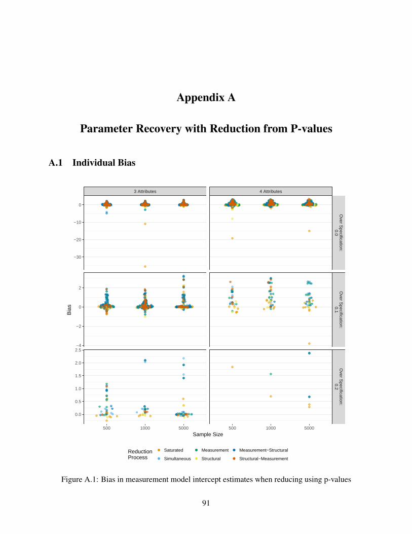
Appendix A
Parameter Recovery with Reduction from P-values
A.1 Individual Bias
3 Attributes 4 Attributes
Over S
pecification:0.0
Over S
pecification:0.1
Over S
pecification:0.2
500 1000 5000 500 1000 5000
−30
−20
−10
0
−4
−2
0
2
0.0
0.5
1.0
1.5
2.0
2.5
Sample Size
Bia
s
ReductionProcess
●
●
●
●
●
●
Saturated
Simultaneous
Measurement
Structural
Measurement−Structural
Structural−Measurement
Figure A.1: Bias in measurement model intercept estimates when reducing using p-values
91
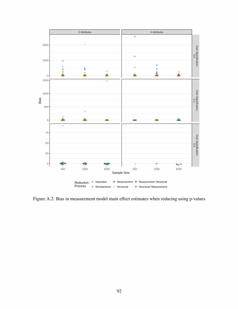
3 Attributes 4 Attributes
Over S
pecification:0.0
Over S
pecification:0.1
Over S
pecification:0.2
500 1000 5000 500 1000 5000
0
1000
2000
0
500
1000
1500
0
25
50
75
Sample Size
Bia
s
ReductionProcess
●
●
●
●
●
●
Saturated
Simultaneous
Measurement
Structural
Measurement−Structural
Structural−Measurement
Figure A.2: Bias in measurement model main effect estimates when reducing using p-values
92
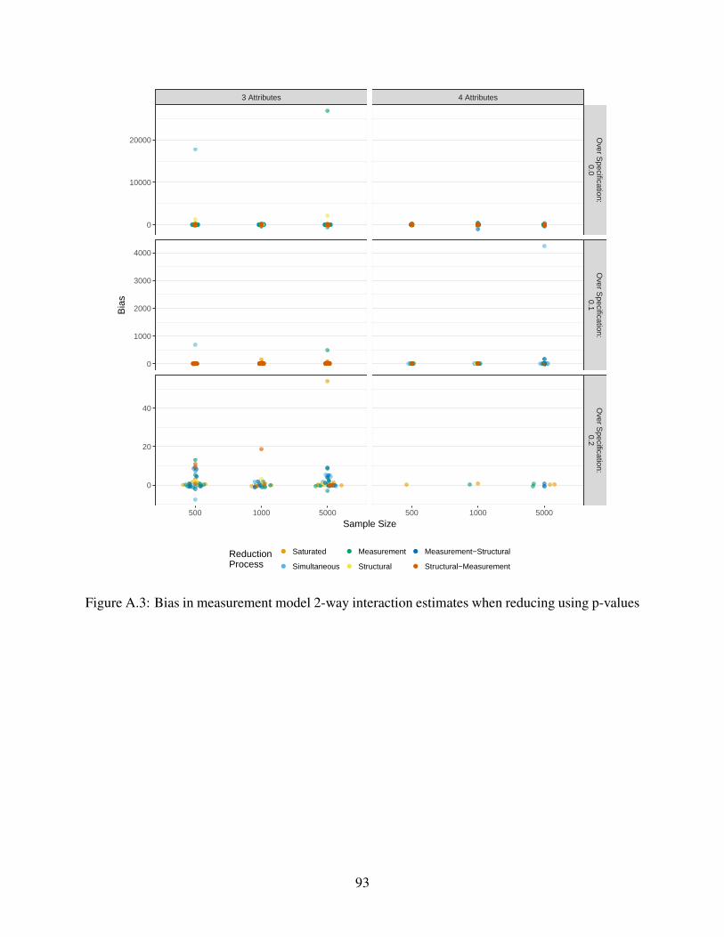
3 Attributes 4 Attributes
Over S
pecification:0.0
Over S
pecification:0.1
Over S
pecification:0.2
500 1000 5000 500 1000 5000
0
10000
20000
0
1000
2000
3000
4000
0
20
40
Sample Size
Bia
s
ReductionProcess
●
●
●
●
●
●
Saturated
Simultaneous
Measurement
Structural
Measurement−Structural
Structural−Measurement
Figure A.3: Bias in measurement model 2-way interaction estimates when reducing using p-values
93
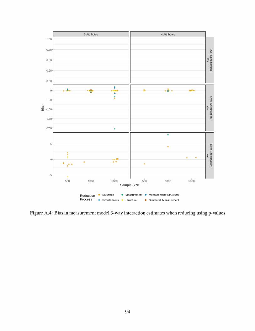
3 Attributes 4 Attributes
Over S
pecification:0.0
Over S
pecification:0.1
Over S
pecification:0.2
500 1000 5000 500 1000 5000
0.00
0.25
0.50
0.75
1.00
−200
−150
−100
−50
0
−5
0
5
Sample Size
Bia
s
ReductionProcess
●
●
●
●
●
●
Saturated
Simultaneous
Measurement
Structural
Measurement−Structural
Structural−Measurement
Figure A.4: Bias in measurement model 3-way interaction estimates when reducing using p-values
94
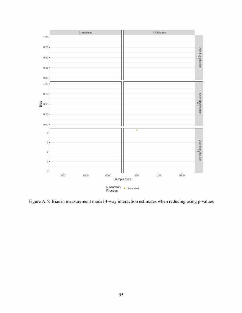
3 Attributes 4 Attributes
Over S
pecification:0.0
Over S
pecification:0.1
Over S
pecification:0.2
500 1000 5000 500 1000 5000
0.00
0.25
0.50
0.75
1.00
0.00
0.25
0.50
0.75
1.00
0
1
2
3
4
Sample Size
Bia
s
ReductionProcess
● Saturated
Figure A.5: Bias in measurement model 4-way interaction estimates when reducing using p-values
95
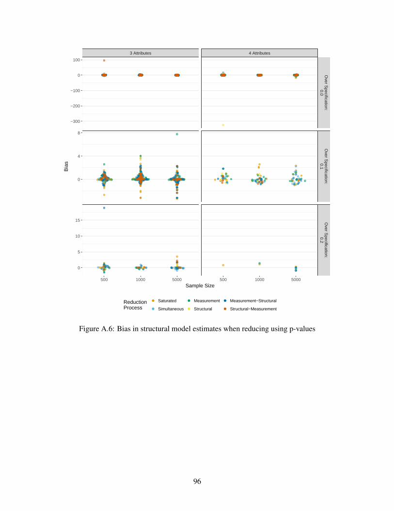
3 Attributes 4 Attributes
Over S
pecification:0.0
Over S
pecification:0.1
Over S
pecification:0.2
500 1000 5000 500 1000 5000
−300
−200
−100
0
100
0
4
8
0
5
10
15
Sample Size
Bia
s
ReductionProcess
●
●
●
●
●
●
Saturated
Simultaneous
Measurement
Structural
Measurement−Structural
Structural−Measurement
Figure A.6: Bias in structural model estimates when reducing using p-values
96
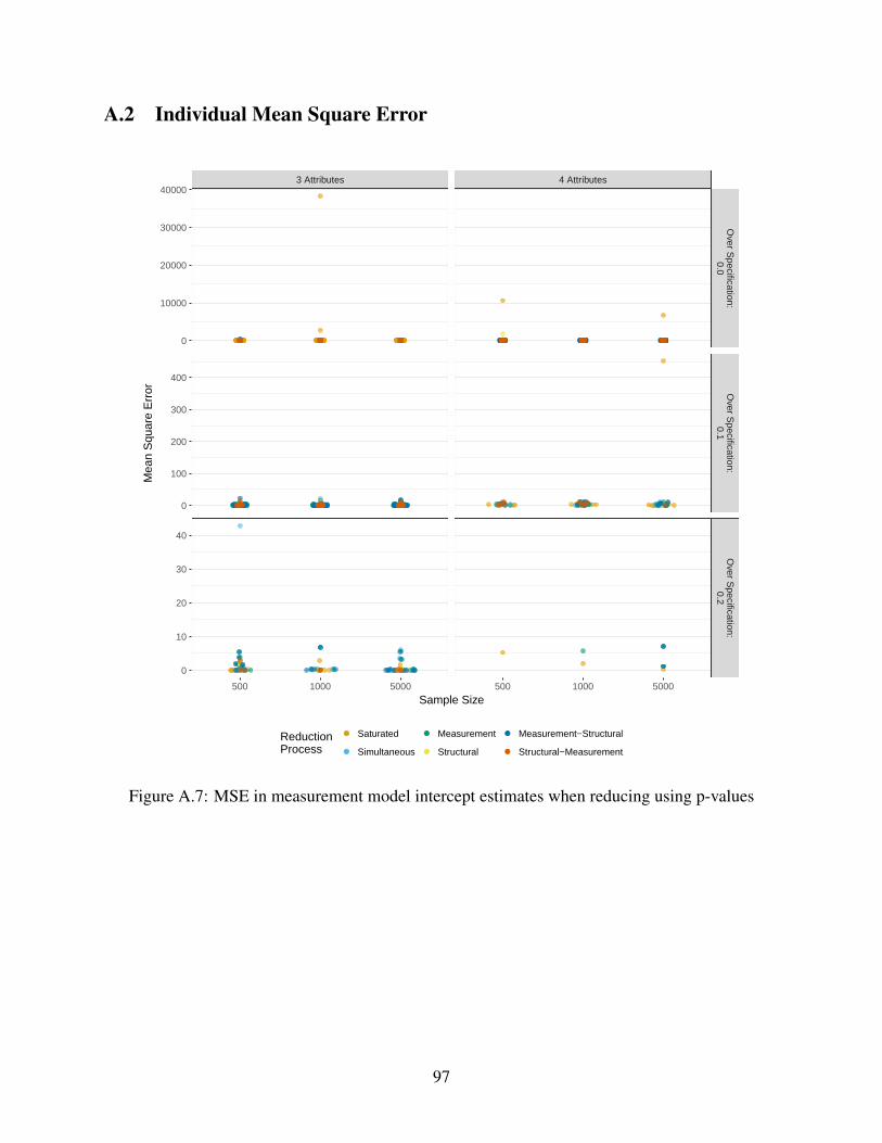
A.2 Individual Mean Square Error
3 Attributes 4 Attributes
Over S
pecification:0.0
Over S
pecification:0.1
Over S
pecification:0.2
500 1000 5000 500 1000 5000
0
10000
20000
30000
40000
0
100
200
300
400
0
10
20
30
40
Sample Size
Mea
n S
quar
e E
rror
ReductionProcess
●
●
●
●
●
●
Saturated
Simultaneous
Measurement
Structural
Measurement−Structural
Structural−Measurement
Figure A.7: MSE in measurement model intercept estimates when reducing using p-values
97
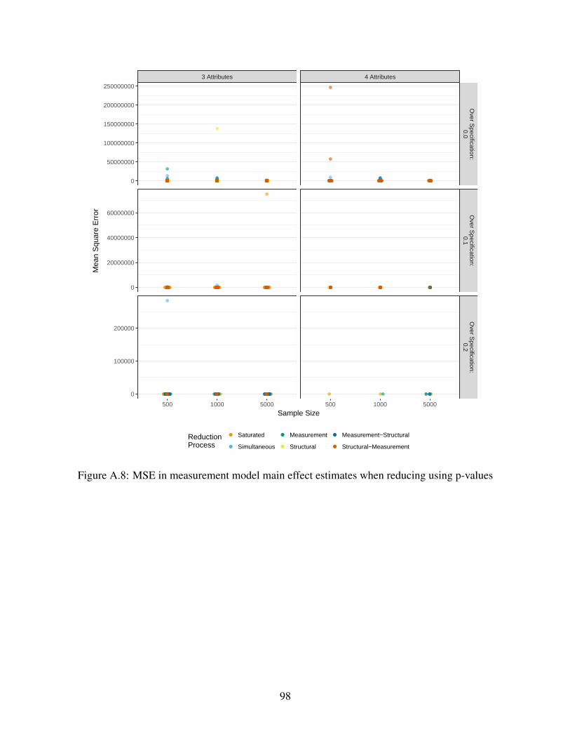
3 Attributes 4 Attributes
Over S
pecification:0.0
Over S
pecification:0.1
Over S
pecification:0.2
500 1000 5000 500 1000 5000
0
50000000
100000000
150000000
200000000
250000000
0
20000000
40000000
60000000
0
100000
200000
Sample Size
Mea
n S
quar
e E
rror
ReductionProcess
●
●
●
●
●
●
Saturated
Simultaneous
Measurement
Structural
Measurement−Structural
Structural−Measurement
Figure A.8: MSE in measurement model main effect estimates when reducing using p-values
98
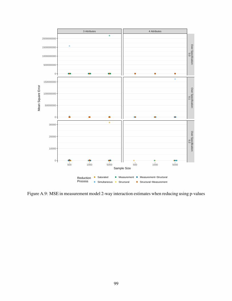
3 Attributes 4 Attributes
Over S
pecification:0.0
Over S
pecification:0.1
Over S
pecification:0.2
500 1000 5000 500 1000 5000
0
500000000
1000000000
1500000000
2000000000
0
50000000
100000000
150000000
0
10000
20000
30000
Sample Size
Mea
n S
quar
e E
rror
ReductionProcess
●
●
●
●
●
●
Saturated
Simultaneous
Measurement
Structural
Measurement−Structural
Structural−Measurement
Figure A.9: MSE in measurement model 2-way interaction estimates when reducing using p-values
99
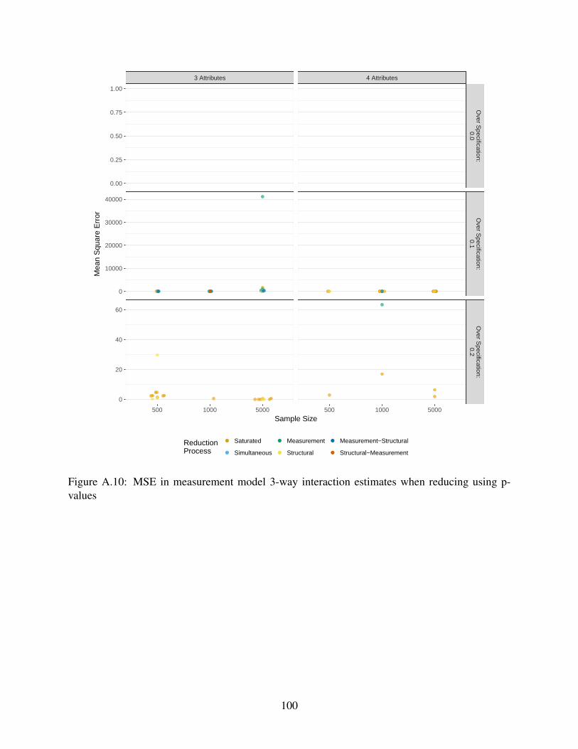
3 Attributes 4 Attributes
Over S
pecification:0.0
Over S
pecification:0.1
Over S
pecification:0.2
500 1000 5000 500 1000 5000
0.00
0.25
0.50
0.75
1.00
0
10000
20000
30000
40000
0
20
40
60
Sample Size
Mea
n S
quar
e E
rror
ReductionProcess
●
●
●
●
●
●
Saturated
Simultaneous
Measurement
Structural
Measurement−Structural
Structural−Measurement
Figure A.10: MSE in measurement model 3-way interaction estimates when reducing using p-values
100
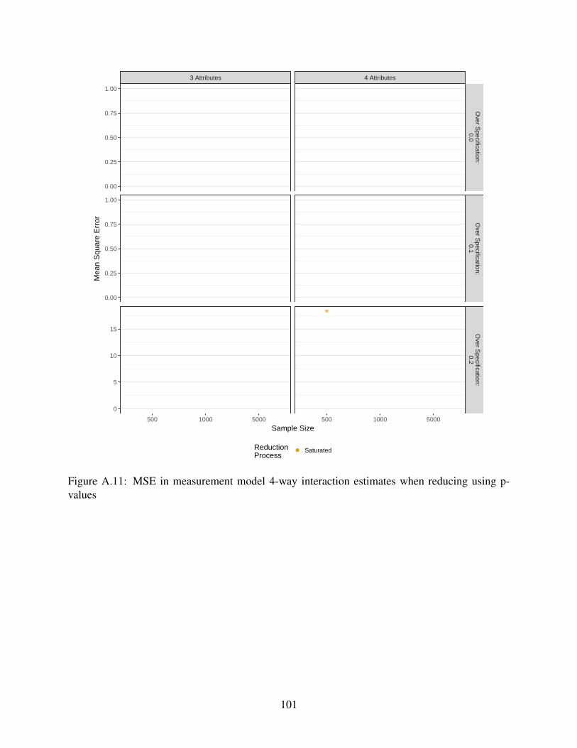
3 Attributes 4 Attributes
Over S
pecification:0.0
Over S
pecification:0.1
Over S
pecification:0.2
500 1000 5000 500 1000 5000
0.00
0.25
0.50
0.75
1.00
0.00
0.25
0.50
0.75
1.00
0
5
10
15
Sample Size
Mea
n S
quar
e E
rror
ReductionProcess
● Saturated
Figure A.11: MSE in measurement model 4-way interaction estimates when reducing using p-values
101
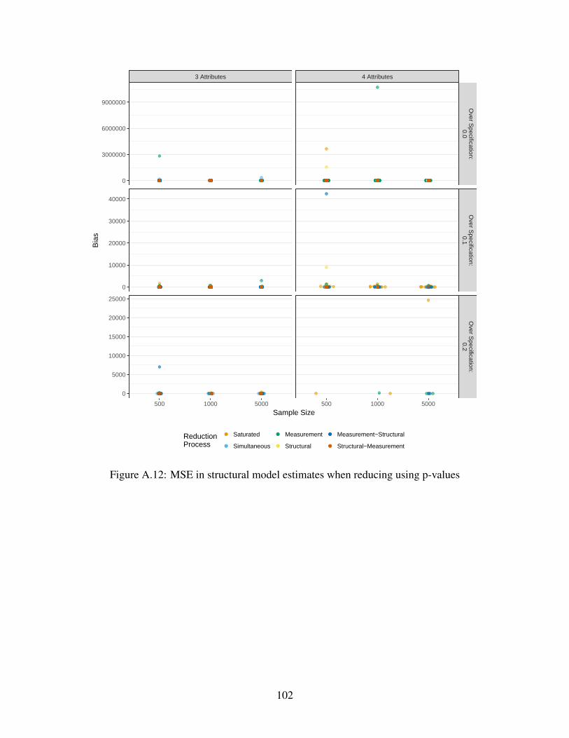
3 Attributes 4 Attributes
Over S
pecification:0.0
Over S
pecification:0.1
Over S
pecification:0.2
500 1000 5000 500 1000 5000
0
3000000
6000000
9000000
0
10000
20000
30000
40000
0
5000
10000
15000
20000
25000
Sample Size
Bia
s
ReductionProcess
●
●
●
●
●
●
Saturated
Simultaneous
Measurement
Structural
Measurement−Structural
Structural−Measurement
Figure A.12: MSE in structural model estimates when reducing using p-values
102
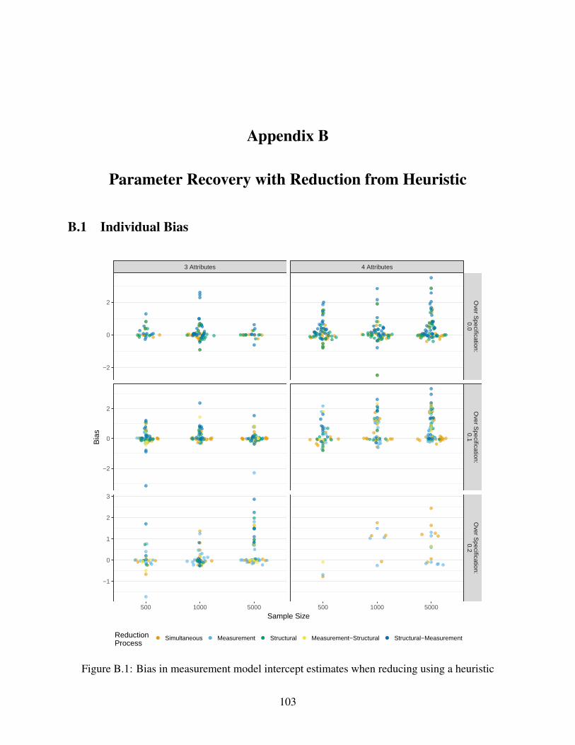
Appendix B
Parameter Recovery with Reduction from Heuristic
B.1 Individual Bias
3 Attributes 4 Attributes
Over S
pecification:0.0
Over S
pecification:0.1
Over S
pecification:0.2
500 1000 5000 500 1000 5000
−2
0
2
−2
0
2
−1
0
1
2
3
Sample Size
Bia
s
ReductionProcess
● ● ● ● ●Simultaneous Measurement Structural Measurement−Structural Structural−Measurement
Figure B.1: Bias in measurement model intercept estimates when reducing using a heuristic
103
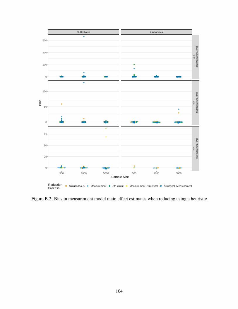
3 Attributes 4 Attributes
Over S
pecification:0.0
Over S
pecification:0.1
Over S
pecification:0.2
500 1000 5000 500 1000 5000
0
200
400
600
0
50
100
0
25
50
75
Sample Size
Bia
s
ReductionProcess
● ● ● ● ●Simultaneous Measurement Structural Measurement−Structural Structural−Measurement
Figure B.2: Bias in measurement model main effect estimates when reducing using a heuristic
104
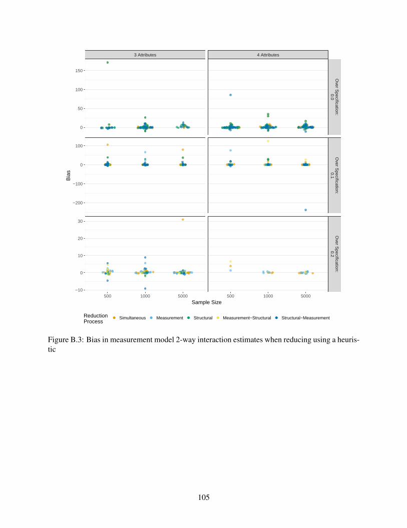
3 Attributes 4 Attributes
Over S
pecification:0.0
Over S
pecification:0.1
Over S
pecification:0.2
500 1000 5000 500 1000 5000
0
50
100
150
−200
−100
0
100
−10
0
10
20
30
Sample Size
Bia
s
ReductionProcess
● ● ● ● ●Simultaneous Measurement Structural Measurement−Structural Structural−Measurement
Figure B.3: Bias in measurement model 2-way interaction estimates when reducing using a heuris-tic
105
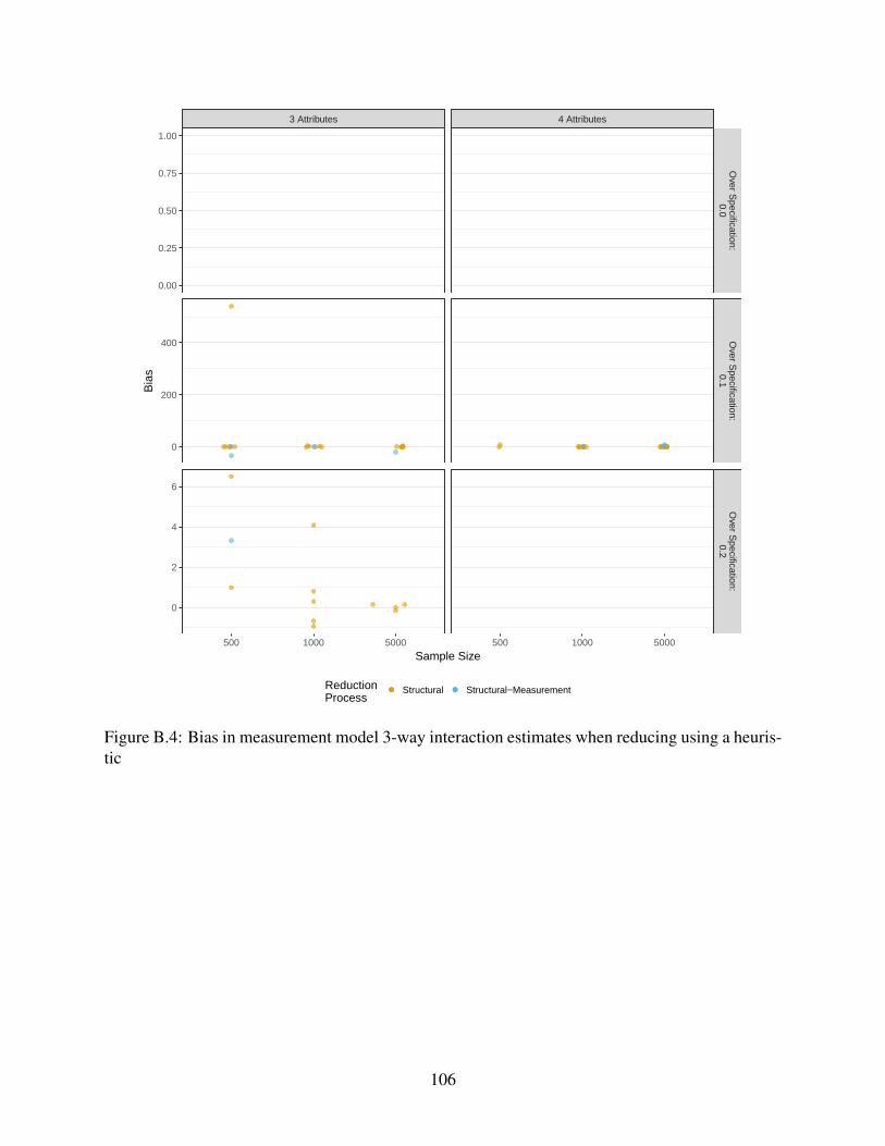
3 Attributes 4 Attributes
Over S
pecification:0.0
Over S
pecification:0.1
Over S
pecification:0.2
500 1000 5000 500 1000 5000
0.00
0.25
0.50
0.75
1.00
0
200
400
0
2
4
6
Sample Size
Bia
s
ReductionProcess
● ●Structural Structural−Measurement
Figure B.4: Bias in measurement model 3-way interaction estimates when reducing using a heuris-tic
106
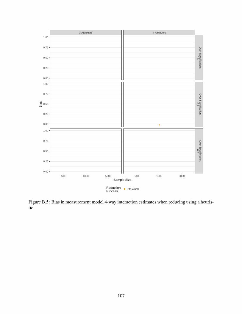
3 Attributes 4 Attributes
Over S
pecification:0.0
Over S
pecification:0.1
Over S
pecification:0.2
500 1000 5000 500 1000 5000
0.00
0.25
0.50
0.75
1.00
0.00
0.25
0.50
0.75
1.00
0.00
0.25
0.50
0.75
1.00
Sample Size
Bia
s
ReductionProcess
● Structural
Figure B.5: Bias in measurement model 4-way interaction estimates when reducing using a heuris-tic
107
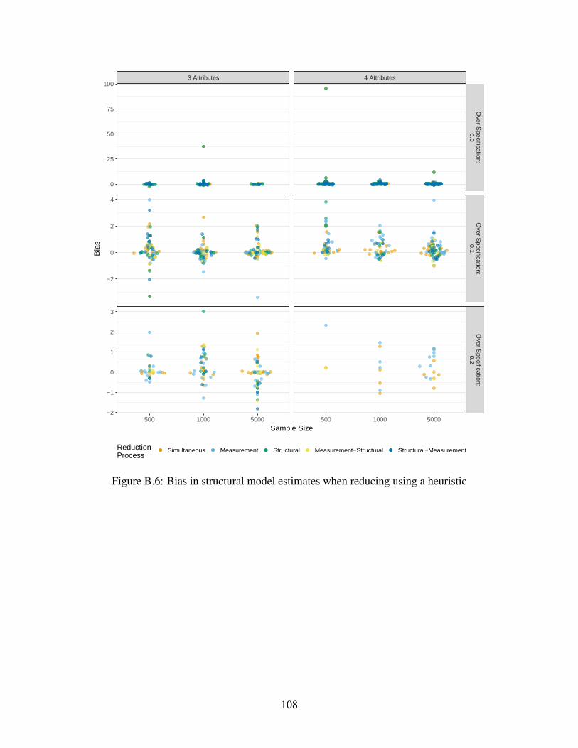
3 Attributes 4 Attributes
Over S
pecification:0.0
Over S
pecification:0.1
Over S
pecification:0.2
500 1000 5000 500 1000 5000
0
25
50
75
100
−2
0
2
4
−2
−1
0
1
2
3
Sample Size
Bia
s
ReductionProcess
● ● ● ● ●Simultaneous Measurement Structural Measurement−Structural Structural−Measurement
Figure B.6: Bias in structural model estimates when reducing using a heuristic
108
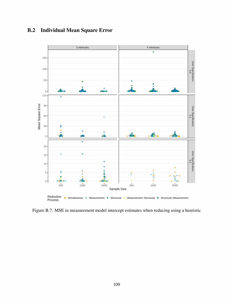
B.2 Individual Mean Square Error
3 Attributes 4 Attributes
Over S
pecification:0.0
Over S
pecification:0.1
Over S
pecification:0.2
500 1000 5000 500 1000 5000
0
50
100
150
0
30
60
90
120
0
5
10
15
20
Sample Size
Mea
n S
quar
e E
rror
ReductionProcess
● ● ● ● ●Simultaneous Measurement Structural Measurement−Structural Structural−Measurement
Figure B.7: MSE in measurement model intercept estimates when reducing using a heuristic
109
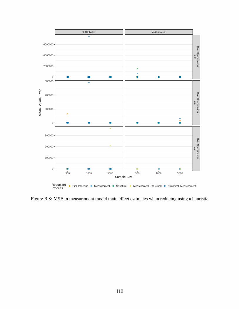
3 Attributes 4 Attributes
Over S
pecification:0.0
Over S
pecification:0.1
Over S
pecification:0.2
500 1000 5000 500 1000 5000
0
2000000
4000000
6000000
0
200000
400000
600000
0
100000
200000
300000
Sample Size
Mea
n S
quar
e E
rror
ReductionProcess
● ● ● ● ●Simultaneous Measurement Structural Measurement−Structural Structural−Measurement
Figure B.8: MSE in measurement model main effect estimates when reducing using a heuristic
110
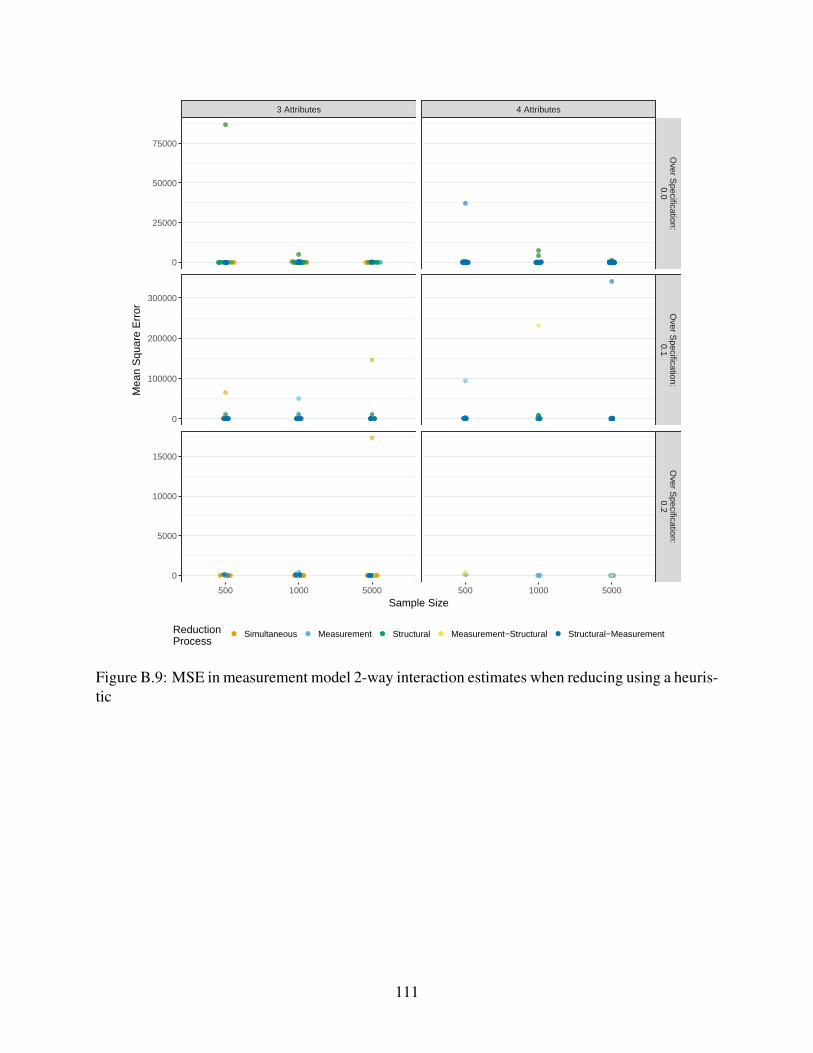
3 Attributes 4 Attributes
Over S
pecification:0.0
Over S
pecification:0.1
Over S
pecification:0.2
500 1000 5000 500 1000 5000
0
25000
50000
75000
0
100000
200000
300000
0
5000
10000
15000
Sample Size
Mea
n S
quar
e E
rror
ReductionProcess
● ● ● ● ●Simultaneous Measurement Structural Measurement−Structural Structural−Measurement
Figure B.9: MSE in measurement model 2-way interaction estimates when reducing using a heuris-tic
111
3 Attributes 4 Attributes
Over S
pecification:0.0
Over S
pecification:0.1
Over S
pecification:0.2
500 1000 5000 500 1000 5000
0.00
0.25
0.50
0.75
1.00
0
100000
200000
300000
0
20
40
60
Sample Size
Mea
n S
quar
e E
rror
ReductionProcess
● ●Structural Structural−Measurement
Figure B.10: MSE in measurement model 3-way interaction estimates when reducing using aheuristic
112
3 Attributes 4 Attributes
Over S
pecification:0.0
Over S
pecification:0.1
Over S
pecification:0.2
500 1000 5000 500 1000 5000
0.00
0.25
0.50
0.75
1.00
0.00
0.25
0.50
0.75
1.00
0.00
0.25
0.50
0.75
1.00
Sample Size
Mea
n S
quar
e E
rror
ReductionProcess
● Structural
Figure B.11: MSE in measurement model 4-way interaction estimates when reducing using aheuristic
113
3 Attributes 4 Attributes
Over S
pecification:0.0
Over S
pecification:0.1
Over S
pecification:0.2
500 1000 5000 500 1000 5000
0
100000
200000
300000
400000
0
5000
10000
15000
20000
0
100
200
300
400
500
Sample Size
Bia
s
ReductionProcess
● ● ● ● ●Simultaneous Measurement Structural Measurement−Structural Structural−Measurement
Figure B.12: MSE in structural model estimates when reducing using a heuristic
114