Evaluating measurement invariance in categorical

data latent variable models with the EPC-interest

DL Oberski JK Vermunt G Moors

Department of Methodology and Statistics

Tilburg University, The Netherlands

Address:

Room P 1105, PO Box 90153, 5000 LE Tilburg

Phone: +31 13 466 2959

Email: d.oberski@tilburguniversity.edu

FUNDING

The first author was supported by Veni grant number 451-14-017 and the second author

by Vici grant number 453-10-002, both from the Netherlands Organization for Scientific

Research (NWO).

ACKNOWLEDGEMENTS

We are grateful to two anonymous reviewers, the editor, Katrijn van Deun, Lianne

Ippel, Eldad Davidov, Zsuzsa Bakk, Verena Schmittmann, and participants of EAM

2014 in for their comments.

Evaluating measurement invariance in categorical

data latent variable models with the EPC-interest

–BLINDED VERSION–

ABSTRACT

Many variables crucial to the social sciences are not directly observed but

instead are latent and measured indirectly. When an external variable of

interest affects this measurement, estimates of its relationship with the

latent variable will then be biased. Such violations of “measurement in-

variance” may, for example, confound true differences across countries in

postmaterialism with measurement differences. To deal with this problem,

researchers commonly aim at “partial measurement invariance”, i.e. to ac-

count for those differences that may be present and important. To evaluate

this importance directly through sensitivity analysis, the “EPC-interest”

was recently introduced for continuous data. However, latent variable mod-

els in the social sciences often use categorical data. The current paper there-

fore extends the EPC-interest to latent variable models for categorical data

and demonstrates its use in example analyses of US Senate votes as well as

respondent rankings of postmaterialism values in the World Values Study.

Program inputs and data for the examples discussed in this article are

provided in the electronic appendix (http://[blinded]).

1

1. INTRODUCTION

Latent variable models for categorical data are commonly used in the social and behav-

ioral sciences, and include well-known special cases such as latent class analysis, item

response theory (IRT), and ordinal factor analysis. Examples of such analyses include

ideological positions of US senators measured by Yea/Nay votes (Poole and Rosenthal,

1985), public tolerance for nonconformity measured by categorical questions in a sur-

vey (McCutcheon, 1985), and postmaterialism measured by respondents’ rankings of

values (Inglehart, 1977; Moors and Vermunt, 2007).

Primary scientific interest in latent variable models often focuses on the relationship

such latent variables have with external variables. For example, on the polarization

of ideology by political party, on education and cohort differences in tolerance, or on

cross-country differences in postmaterialism. However, if the measurement of the latent

variable differs over values of such external variables, relationship estimates of interest

may be biased (Steenkamp and Baumgartner, 1998). Thus, “measurement invariance”

is needed to estimate such relationships.

For this reason, whenever the aim is to compare values of the latent variable, it is

common practice to perform “measurement invariance testing” (see Vandenberg and

Lance, 2000; Schmitt and Kuljanin, 2008, for reviews), a practice also known as testing

for “differential item functioning” (DIF) in the IRT literature (Holland and Wainer,

1993). That is, detecting any observed indicators that might violate measurement in-

variance and accounting for these violations in the model. The aim of measurement

invariance testing is to ensure the comparability of latent variable scores over values of

an external variable. However, currently existing procedures do not necessarily reach

this aim because they do not account for the substantive impact of violations of mea-

surement invariance on the relationship parameters of interest (Oberski, 2014).

2

To this end, Oberski (2014) suggested supplementing measurement invariance test-

ing for linear structural equation models with sensitivity analysis. Sensitivity analysis

investigates directly the impact of measurement invariance violations on the relation-

ship parameters of interest. It can be performed by fitting many alternative models,

with the disadvantage that this process will sometimes be infeasible. Oberski (2014)

therefore also introduced the EPC-interest, a measure that approximates the change in

parameters of interest without the need to fit alternative models. Since EPC-interest

was only introduced for continuous data linear structural equation models, however, it

is not applicable to categorical data analyses such as those described above.

In this paper we therefore extend the EPC-interest approach to measurement in-

variance testing to the case of categorical data latent variable models. The extended

measure is evaluated in a small simulation study, and its use demonstrated in two ex-

ample applications. In the first of these applications the polarization of the 90th US

senate is examined by applying an ideal point model; the second application analyzes

the rankings of value priorities given by 67,568 WVS respondents in 48 countries.

Section 2 explains categorical data latent variable models and the problem of mea-

surement invariance. The EPC-interest is introduced in Section 2.3 as an approxi-

mation to the sensitivity analysis approach to measurement invariance testing and a

small simulation study evaluates the approximation in Section 2.4. Sections 3 and 4

then elaborate the two example applications, while Section 5 concludes.

3

2. MEASUREMENT INVARIANCE IN CATEGORICAL DATA

2.1. The problem of measurement invariance

Many important variables in the social sciences are not or cannot be directly observed,

but are instead latent (Bollen, 2002) and measured using a vector of multiple indicators,

y, say. This measurement of the latent variable x is defined by a “measurement model”,

p(y|x). (1)

The latent x variable could, for example, be a “random effect”, a person’s unobserved

utility for a choice, a general attitude, or a variable measured with error such as voter

turnout. Often the measurement model in Equation 1 is not, however, of primary

interest to the researcher, but rather the relationship between the latent variable and

some covariate vector z is, i.e. the “structural model”,

p(x|z). (2)

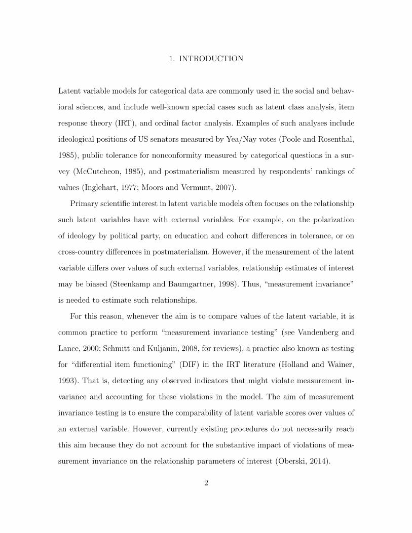
Figure 1 shows this relationship as an arrow between the observed covariate z and

latent variable x. For example, z could contain a set of dummy variables indicating a

respondent’s country or gender, so that Equation 2 simply compares values of x across

countries or genders. Alternatively, interest could focus on the influence of continuous

covariates such as GDP or age on the latent x. Of course, the problem is that x is not

observed, but only y and z are.

Latent variable models generally attack this problem by making two key assump-

tions about how x is measured (Skrondal and Rabe-Hesketh, 2004). The first assump-

4

x or to a difference over the covariate in the way x is measured. For example, when

comparing countries, an observed cross-country difference in anti-immigrant attitudes

might be a substantive difference or it might equally well be explained as differing

answer tendencies over countries.

This identification problem only occurs, however, when there are no measurement

invariant indicators at all. A single invariant indicator can disentangle measurement

from substantive differences in the other, non-invariant, indicators. Full measurement

invariance is therefore not necessary to identify the structural model, but “partial mea-

surement invariance” is (Byrne, Shavelson and Muthen, 1989). The standard practice

is to search for non-invariant indicators and either remove them or parameterize their

differential functioning (Holland and Wainer, 1993). A common way of doing so when

the observed variables are categorical with K categories is a logistic regression,

P (Yj = k) =exp(τjk + λjkx+ δjkz)∑

m∈{1..K} exp(τjm + λjmx+ δjmz), (4)

(Mellenbergh, 1989; Kankaras, Moors and Vermunt, 2010), where some restriction is

imposed on the parameters for identification purposes such as “effect coding”,∑

k τjk =∑k λjk =

∑k δjk = 0, or dummy coding, τj1 = λj1 = δj1 = 0. It can be seen in Equation

4 that setting δjk = 0 corresponds to measurement invariance1. This means that it is

possible to estimate a model in which δjk 6= 0 for some indicators, while δjk is kept

at zero, i.e. partially measurement invariant, for others. Figure 1 shows this possible

direct effect from covariate to indicator as a dashed arrow.

1An interaction term δ∗jkzx could be added to Equation 4 but has been omitted for clarity.

6

2.2. Existing solutions

In short, some form of measurement invariance is needed to estimate the structural

model of interest: deciding which form, that is, selecting a model, is therefore crucial.

Currently, there are broadly three existing approaches to doing so:

1. Selecting one indicator as the reference indicator or “anchor item” a priori ;

2. Imposing a strong prior on the differential functioning parameters (Muthen and

Asparouhov, 2012);

3. Testing the null hypothesis of full measurement invariance (Steenkamp and Baum-

gartner, 1998; French and Finch, 2006) or partial measurement invariance, in

which violations of invariance are freed (Byrne, Shavelson and Muthen, 1989;

Saris, Satorra and Van der Veld, 2009).

A priori reference indicators are often selected implicitly, for example by setting

one loading to unity in multiple group CFA. A recent extension to this approach, the

“alignment method”, was suggested by Muthen and Asparouhov (2014). When the

researcher is not certain that the “reference indicator” is indeed invariant, however, it

is impossible to select it based on the data (Hancock, Stapleton and Arnold-Berkovits,

2009). The Bayesian approach suggested by Muthen and Asparouhov (2012) has the

distinct advantage that, when the prior has been chosen aptly, the data can determine

which indicators should be more or less invariant – hence the term “approximate mea-

surement invariance” (see also Van De Schoot et al., 2013). However, if the prior is not

chosen adequately, for instance if it is too strong or too weak, bias in the parameters

of interest may still occur. At current this remains a topic for future study, although

the approach is promising. Finally, it is common to test for full or partial measurement

7

invariance using various fit measures available for this purpose (Byrne, Shavelson and

Muthen, 1989; Hu and Bentler, 1998; Cheung and Rensvold, 2002; Chen, 2007; Saris,

Satorra and Van der Veld, 2009). However, this approach has recently been shown to

have an unfortunate disadvantage: when a violation is detected, it need not have se-

riously affected the parameter of interest, and when an invariance model is selected,

substantial bias in the parameter of interest may still remain (Oberski, 2014). In short,

while measurement invariance is an important assumption in latent variable model-

ing, the existing methods do not directly account for the effect that violations of this

assumption have on the parameters of interest.

To complement measurement invariance testing, the EPC-interest was therefore

recently introduced by Oberski (2014) for continuous data structural equation models.

The EPC-interest assesses what would happen if a particular possible direct effect

were freed. Rather than assessing the size of this direct effect itself, however, it assesses

its impact on the parameter of interest. However, this measure is only available for

continuous data, whereas many important measures of latent variables in the social

sciences are categorical. Examples include the votes (Yea/Nay) of senators indicating

their ideology, how respondents rank their value priorities (1 through 4), or answers

(correct/incorrect) to political knowledge questions. The following section therefore

extends the EPC-interest to the case of categorical indicators.

2.3. EPC-interest

The “EPC-interest” estimates the change in a free parameter estimate of the model

that one can expect to observe if a particular restriction were freed. It is therefore a

method of sensitivity analysis. However, the researcher is not forced to estimate all

possible alternative models, but can evaluate the sensitivity of the results after fitting

8

the restrictive full invariance model. The EPC-interest is based on the work of Saris,

Satorra and Sorbom (1987), who introduced the expected parameter change in a fixed

parameter for linear structural equation models (SEM), and Bentler and Chou (1993),

who introduced the expected parameter change in a free parameter after freeing a

fixed parameter for SEM. It was applied to invariance testing with continuous data by

Oberski (2014).

In models for categorical data, the EPC-interest can be derived, as shown below

and in the Appendix, by applying general results of maximum likelihood analysis. An

additional problem with categorical data, however, is that there is usually a large set

of parameters relating to a particular variable. For example, in Equation 4, there will

be K “loadings” λjk, K “intercepts” τjk, K “direct effects” δjk, and, if present, K

“interaction effects” δ∗jk for each variable. These parameters will, moreover, be strongly

dependent on one another, so that the impact of freeing one of them cannot be seen

separately from the impact of freeing another parameter relating to the same variable.

For this reason, when extending EPC-interest to the categorical case, it also becomes

necessary to allow for the consideration of sets of parameters to free rather than just

investigating the effect of single restrictions.

In deriving the EPC-interest, the key concept is considering the likelihood not

only as a function of the free parameters of the model, but also as a function of

the parameters that are fixed to obtain the full invariance model. Collecting the free

parameters in a vector θ and the fixed parameters in a vector ψ, we assume the

likelihood can be written as an explicit function of both sets of parameters, L(θ,ψ). The

maximum-likelihood estimates θ of the free parameters can then be seen as obtained

under the full invariance model that sets ψ = 0, i.e. θ = arg maxθ L(θ,ψ = 0). Further,

define the parameters of substantive interest as π := Pθ, where P is typically a logical

(0/1) selection matrix, although any linear function of the free parameters θ may be

9

taken. Interest then focuses on the likely value these free parameters π would take if

the fixed ψ parameters were freed in an alternative model, πa = P arg maxθ,ψ L(θ,ψ).

We now show how these changes in the parameters of interest as a consequence of

freeing the fixed parameters ψ can be estimated without fitting the alternative model.

Let the Hessian Hab be the matrix of second derivatives of the likelihood with respect

to vectors a and b, evaluated at the maximum likelihood solution of the full invariance

model, Hab := (∂2L/∂a∂b′)|θ=θ. The expected change in the parameters of interest is

then measured by the EPC-interest,

EPC-interest = πa − π = PH−1θθ HθψD

−1[∂L(θ,ψ)

∂ψ

∣∣∣∣θ=θ

]+O(δ′δ), (5)

where D := Hψψ− H′θψH

−1θθ Hθψ and the deviation from the true values is δ := ϑ− ϑ,

with ϑ collecting the free and fixed parameters in a vector, ϑ := (θ′,ψ′)′. Note that,

apart from the order of approximation term O(δ′δ), Equation 5 contains only terms

that can be calculated after fitting the invariance model. Thus, it is not necessary to

fit the alternative model to obtain the EPC-interest.

In the structural equation modeling literature, the expected change in the fixed

parameters ψ is commonly found and implemented in standard SEM software. This

measure is commonly know as the “EPC”, but to avoid confusion we term it “EPC-self”

here. The EPC-self and EPC-interest both consider the impact of freeing restrictions,

but differ in the target of this impact: the EPC-self evaluates the impact on the re-

striction itself, whereas the EPC-interest evaluates the impact on the parameters of

interest. In spite of these differences, the two measures are related: this can be seen by

recognizing that −D−1[

∂L(θ,ψ)∂ψ

∣∣∣θ=θ

]= EPC-self ≈ ψ − ψ so that, from Equation 5,

EPC-interest = −PH−1θθ Hθψ EPC-self ≈ −PH

−1θθ Hθψ

(ψ − ψ

)(6)

10

Furthermore, since ψ and θ are implicitly related by the fact that they are both

solutions to the equation ∂L/∂ϑ = 0, invoking the implicit function theorem yields

−H−1θθ Hθψ = ∂θ/∂ψ′, so that

EPC-interest = P

(∂θ

∂ψ′

)(ψ − ψ

), (7)

that is, the EPC-interest can be seen simply as the coefficient of a linear approximation

to the relationship between the free and fixed parameters, multiplied by the change

in the fixed parameters. This demonstrates the difference with the sensitivity analysis

approach common in econometrics (Magnus and Vasnev, 2007, p. 168) in which only

∂θ/∂ψ′ is considered: the EPC-interest combines both the direction (∂θ/∂ψ′) and the

magnitude (ψ − ψ) of the misspecification.

The accuracy of the approximation of the EPC-interest as a measure of the change

in the parameters of interest is reflected in the order of approximation term, O(δ′δ). It

can be seen that this accuracy is quadratic in the overall change in parameters, so that

the approximation can be expected to work best when the misspecifications are not

“too large”. This result corresponds to results on the score test (“modification index”)

and “EPC-self” in the literature on structural equation modeling, which can be shown

to be exact under a “sequence of local alternatives”, i.e. when ϑ = limn→∞ ϑ + n−12δ

(Satorra, 1989, p. 135). It is important to note here that δ is the deviation from the

“true” value of ϑ, rather than the deviation from the limit of the parameter estimates

under the alternative model. Therefore another view on the accuracy is that it will be

better when the alternative model is not strongly misspecified. For this reason it is also

important to consider freeing sets of very strongly related parameters simultaneously,

since a change in one of them will then imply a change in the others, and, consequently,

a misspecified alternative model.

11

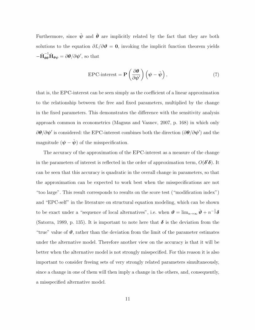
n 250 500 1000True δ 0 0.5 1 0 0.5 1 0 0.5 1

Est. γ 1.010 1.151 1.353 0.980 1.152 1.330 1.013 1.163 1.327Bias γ -0.010 -0.151 -0.353 0.020 -0.152 -0.330 -0.013 -0.163 -0.327EPC-int. 0.003 -0.166 -0.494 -0.001 -0.180 -0.486 0.004 -0.182 -0.448

Table 1: Simulation study of EPC-interest. Shown is the average point estimate for theγ parameter of interest under full measurement invariance (“Est”), its difference fromthe true value γ = 1 (“Bias”), and the average EPC-interest.

2.4. Small simulation study

To demonstrate the extent of the approximation bias in the EPC-interest, we performed

a small simulation study. In this study, we specified a latent variable model for four

binary indicators: P (Yj = 1|x) = [1 + exp(−x)]−1, with j ∈ {2, 3, 4}, and structural

model x = γz + ε with γ = 1 and ε ∼ N(0, 1). We then introduced a violation of

measurement invariance for the first indicator, P (Y1 = 1|x) = [1 + exp(−x − δz)]−1.

Nine conditions varied sample size, n ∈ {250, 500, 1000}, and the size of the invariance

violation: δ = 0 (no violation), 0.5 (moderate), or 1 (extreme). Data were generated

using R 3.1.2 and analyzed using Latent GOLD 5.0.0.14161.

The results over 200 samples are shown in Table 1. The first two rows show the

average point estimate of the parameter of interest γ, and its deviation from the true

value γ = 1, respectively. It can be seen that a modest violation δ = 0.5 still has a

substantively important impact on bias. Under this condition, the amount of bias is

reasonably well approximated by the EPC-interest, which has average values close to

the true bias. When the violation is extreme, however, the approximation causes the

EPC-interest to somewhat overestimate the bias: for example, in the last column of

the table the true bias is -0.327 but EPC-interest estimates it at about -0.448. This

effect appears to be strongest with the smallest sample size, a phenomenon that can

be explained by the approximation term being more likely to take on large values in

12

small samples.

Overall, the results of this very limited simulation study demonstrate the analytic

results discussed above. As expected, for small samples and very large violations of

invariance, the EPC-interest will overestimate the bias caused somewhat. In these

cases, the EPC-interest is still a useful guide but the researcher may wish to verify

that after freeing the violation in question, the results of interest do indeed change

substantially. Alternatively, where this is feasible, one may also resort to estimating

all alternative models and examining the results. In other conditions, the EPC-interest

performs as expected: when there is no bias, it estimates zero on average, and when

there is moderate bias in the parameter of interest, EPC-interest approximates this

bias adequately.

3. EXAMPLE APPLICATION #1: 90TH US SENATE ROLL CALL DATA

To exemplify the use of the EPC-interest using a relatively simple latent variable model

with categorical variables that is well-known in political science, we estimate an ideal

point model on roll call data for senators in the 90th US Senate, which met from 1967

to 1969 during the Lyndon B. Johnson Administration.

The probability that senator i votes “Yea” on motion j is modeled as a logistic

regression on the motion’s (unobserved) utility,

P (“Yea” on motion j|xi) = [1 + exp(−βjuij)]−1, (8)

where the utility uij of the motion to that senator is simply the Euclidean distance

13

between the senator’s position xi and the motion’s position τj,

uij = (xi − τj)2. (9)

This model is equivalent to the well-known unidimensional Poole and Rosenthal (1985)

(W-NOMINATE) model. The latent value xi is known as an “ideal point”.

The Poole-Rosenthal model can be extended to incorporate covariates that predict

the latent variable xi, for example using the party of the senator as a predictor:

xi = α + γ · Party + εi. (10)

Using party (Democratic or Republican) as a predictor allows the researcher to see how

strongly party membership relates to senators’ ideological positions, which ultimately

influences their votes. A higher value of γ thus indicates more ideological homogeneity

within parties in the Senate: we therefore call γ the “polarization coefficient”.

The usual choice εi ∼ Normal(0, σ2) leads to a quadratic structural equation model

(SEM) for categorical data, or, equivalently, a quadratic 2PL IRT model with a co-

variate (Rabe-Hesketh, Skrondal and Pickles, 2004). Alternatively, the distribution of x

can be estimated from the data by choosing some number K of categories for x (“latent

classes”) and modeling the probability of belong to class k as an ordered multinomial

regression,

P (xi = k|Party) =exp(αk + γ · x(k) · Party)∑K

m=1 exp(αm + γ · x(m) · Party), (11)

where x(k) is a latent score assigned to the k-th category of x. For this arbitrary choice

of latent scale, we choose x(k) to go from 0 to 1 in equally spaced intervals (following

Vermunt and Magidson, 2013). The latent category intercepts αk allow the distribution

of the latent dimension to be freely estimated rather than assumed Normal. This leads

14

to the “latent class factor model” (Vermunt and Magidson, 2004).

A possible problem when using ideal point models to investigate polarization is

that it is assumed that this polarization is the same on all motions the Senate votes

on. If there is some motion on which the votes of senators from the same party are

significantly more tight-knitted than usual, there will be an effect of Party over and

above that of the senator’s utility for this motion. A vote model with a direct covariate

effect,

P (“Yea” on motion j|xi) = [1 + exp(−βjuij − δj · Party)]−1, (12)

then replaces Equation 8. In other words, the usual ideal point model assumes mea-

surement invariance with respect to the covariate, an assumption that can be expressed

as δj = 0. Where such direct effects do exist they are relevant to the investigation of

polarization insofar as ignoring them biases the estimate of the Senate’s overall polar-

ization. Thus, we investigate whether the assumption of measurement invariance δj = 0

seriously affects the estimate of interest γ using the EPC-interest.

Maximum likelihood estimates of the parameters were obtained using the software

Latent GOLD, taking K = 4 and the first 20 motions introduced in the 90th Senate

as an example. The model appears to fit the data well, with an L2 bootstrapped p-

value of 0.14, The factor scores xi obtained from this simple model correlated highly

(0.79) with those obtained from W-NOMINATE (Poole et al., 2008) and from Optimal

Classification Roll Call Scaling (0.81; Poole et al., 2012). Based on the full invariance

model, the polarization coefficient γ was estimated at 4.164 (s.e. 1.3077). Since γ is a

logistic regression coefficient, a Republican senator has about four times higher odds

of being one category above a Democratic senator than of being in the same category2.

There was therefore considerable polarization in the 90th Senate.

2Because there are four x categories scored {0, 1/3, 2/3, 1}, the odds are exp(γ/3) ≈ 4.

15

EPC−interest and p−values for consequences ofdifferential measurement error with respect to Party

Fa se d scovery rate adjusted p va ues

EP

C−

inte

rest

01

02

03

04 0506

07

0809

011 12

13

1415

16 1718 19

20

0 .05 .5 .8

1.56

0.78

0.00

0.78

1.56

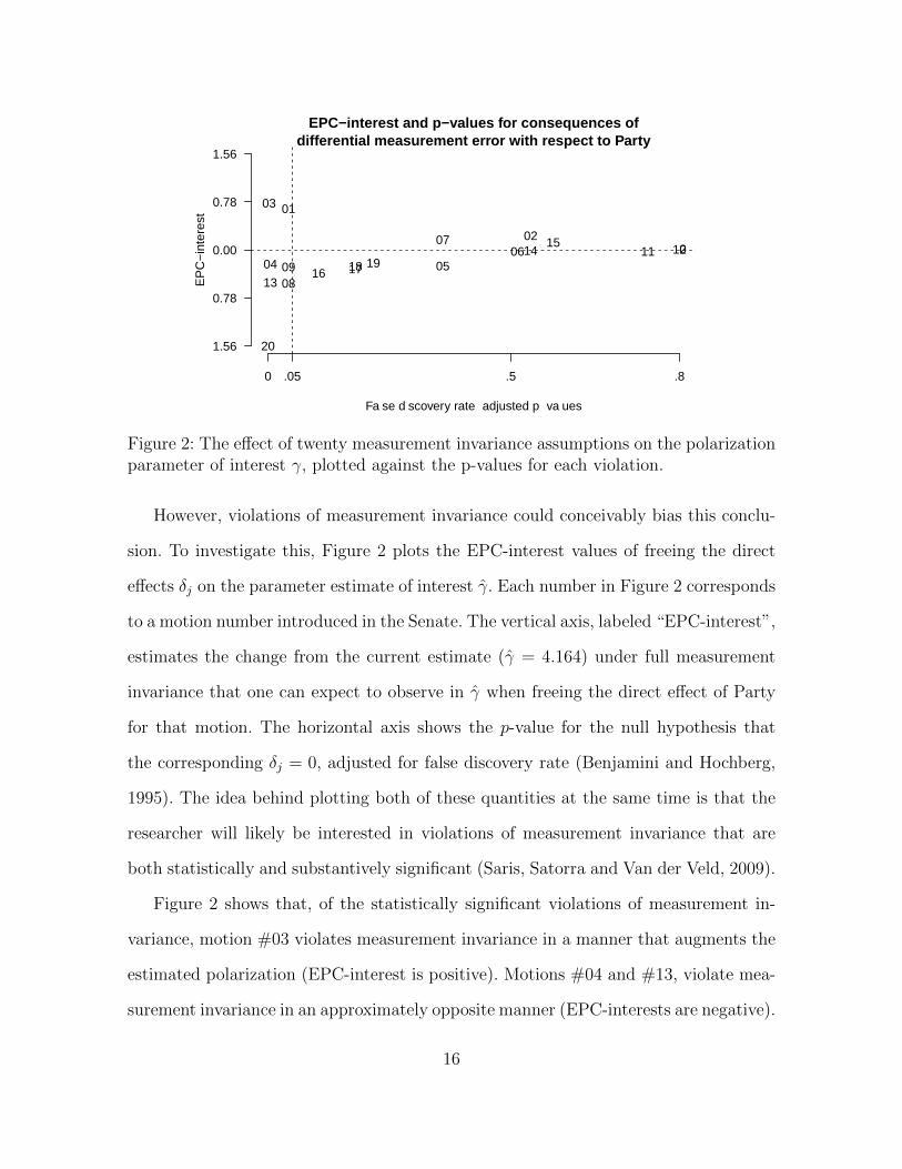
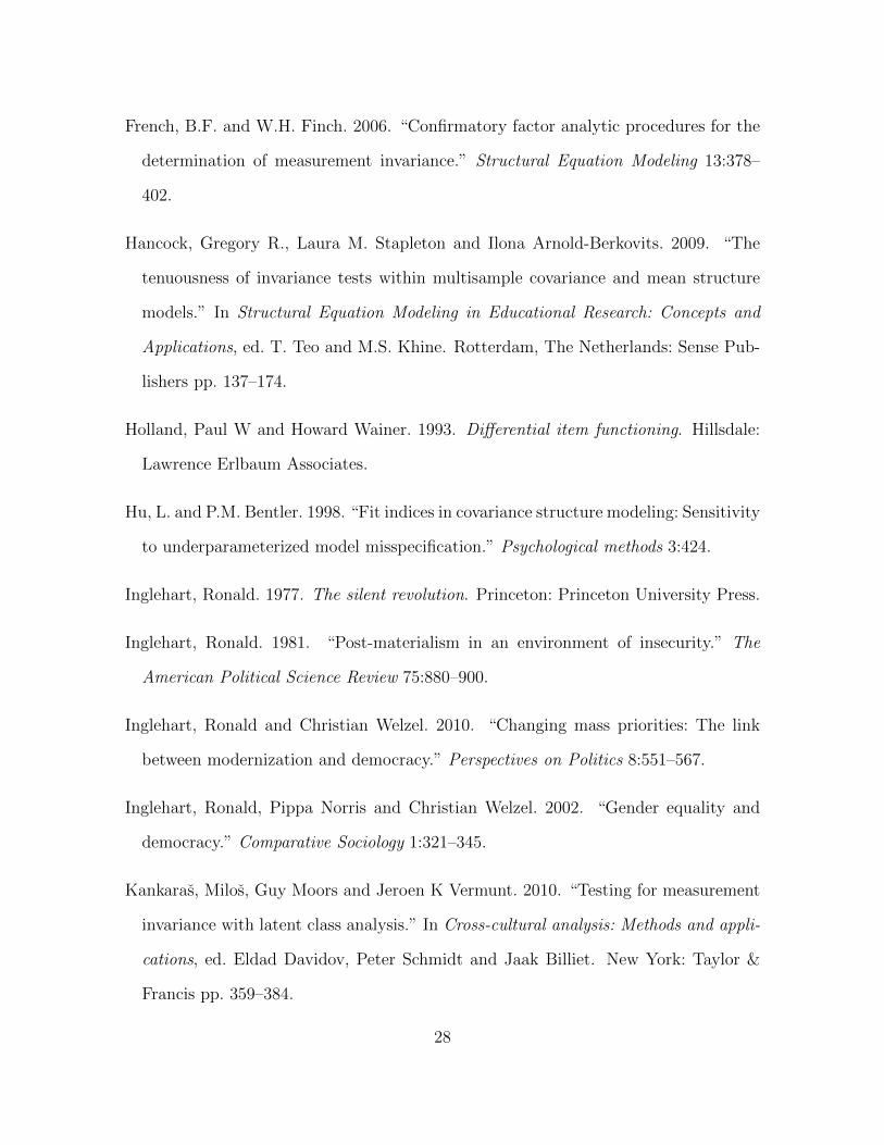
Figure 2: The effect of twenty measurement invariance assumptions on the polarizationparameter of interest γ, plotted against the p-values for each violation.

However, violations of measurement invariance could conceivably bias this conclu-

sion. To investigate this, Figure 2 plots the EPC-interest values of freeing the direct

effects δj on the parameter estimate of interest γ. Each number in Figure 2 corresponds

to a motion number introduced in the Senate. The vertical axis, labeled “EPC-interest”,

estimates the change from the current estimate (γ = 4.164) under full measurement

invariance that one can expect to observe in γ when freeing the direct effect of Party

for that motion. The horizontal axis shows the p-value for the null hypothesis that

the corresponding δj = 0, adjusted for false discovery rate (Benjamini and Hochberg,

1995). The idea behind plotting both of these quantities at the same time is that the

researcher will likely be interested in violations of measurement invariance that are

both statistically and substantively significant (Saris, Satorra and Van der Veld, 2009).

Figure 2 shows that, of the statistically significant violations of measurement in-

variance, motion #03 violates measurement invariance in a manner that augments the

estimated polarization (EPC-interest is positive). Motions #04 and #13, violate mea-

surement invariance in an approximately opposite manner (EPC-interests are negative).

16

However, motion #20, clearly stands out as an important violation of measurement

invariance. After introducing the direct effect of party on voting “Yea” to Motion #20

(freeing δ20), no other measurement invariance violations are statistically significant

(all false discovery rate-adjusted p-values ≥ 0.05). Thus, it seems that Motion #20

(HR4573, which increased the public debt limit) was an issue on which the ranks were

closed more than usual. Indeed, the 1967 CQ Almanac3 specifically reports on this

motion, remarking that “Republicans launched their first major attacks in the 90th

Congress on the Administration’s fiscal policies”, with no Republicans voting in favor.

After adjusting for this event, the polarization coefficient is estimated at 3.422 (s.e.

1.0630): the tight-knittedness between party membership and voting pattern is there-

fore somewhat loosened, but still strong. The partial invariance model after accounting

for this one violation becomes acceptable, in the sense that those violations that are

present do not substantially change the results of interest regarding polarization. The

model fit the data well with an L2 bootstrapped p-value of 0.11. Its BIC (1379) indicates

an improvement over that of the full invariance model (1405). Overall, the difference

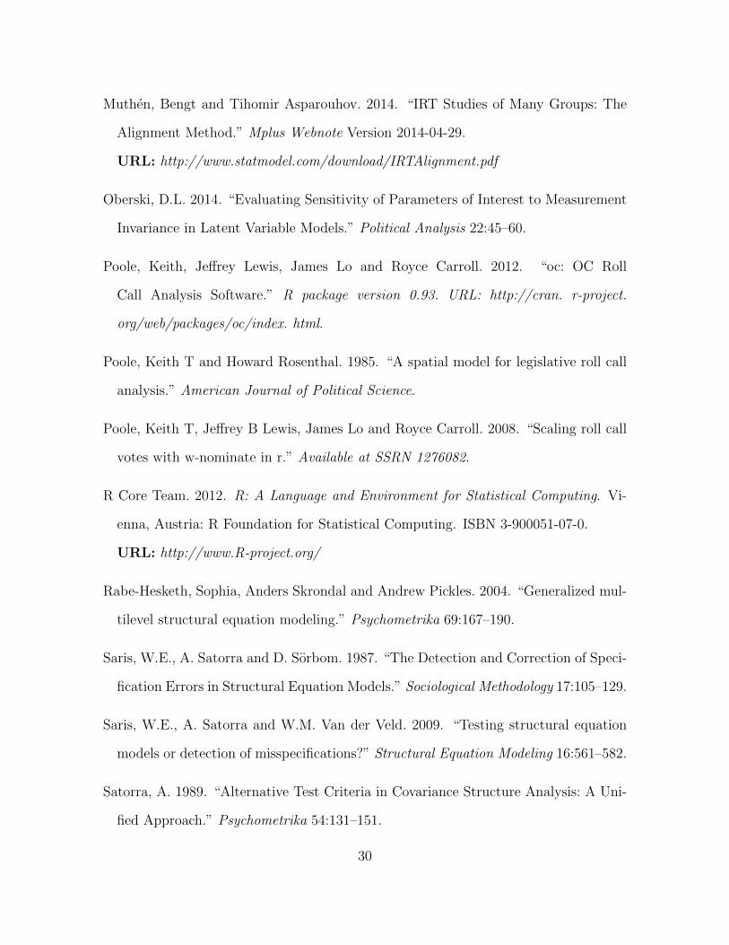
between the fully and partially invariant models are modest. Figure 3 shows the effect

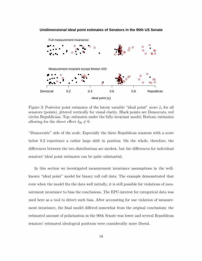
of freeing δ20 on the “ideal point” estimates, i.e. the latent variable estimates xi.

The top part of Figure 3 shows the ideal point estimates under the full invariance

model. These estimates range from zero to one; since Democrats, shown as black dots,

are predominantly on the lower side of the scale, zero has been labeled “Democrat” and

the score 1 has been labeled “Republican”, since most Republicans (red circles) can be

found here. To make the points more visible, they have been jittered randomly in the

vertical direction. The bottom part of Figure 3 shows the ideal point estimates for the

same senators, but this time while accounting for the partial violation of measurement

invariance δ20 6= 0. It can be seen that Republicans are more spread out into the

3http://library.cqpress.com/cqalmanac/document.php?id=cqal67-1314297

17

●

●●

●

●

●

●●

●

●●

●

●

●

●

●●

●●

●●

●

●

●●

●●

●

●●●

●

●

●●

●●

●●

●

●●

●

●

●

● ●●

●

●

●

●

●

●

●

●●

●

●

●

●●

●

●

●

●

● ●●

●●

●

●

●

●

●

●

●

●

●●

●

●

●●

● ●●

●

●●● ●

●

● ● ●

●

●

●

●

Unidimensional ideal point estimates of Senators in the 90th US Senate

Ideal point (xi)

●

●●

●

●

●

●●

●

●●

●

●

●

●

●●●●

●●●

●●

●●

●

●●●

●

●

●●

●●

●●

●

●●

●

●

●

● ●●

●

●

●

●

●

●

●

●●

●

●

●

●●

●

●

●

●

● ●●

●●

●

●

●

●

●

●

●

●

●●

●

●

●●

● ●●

●

●●● ●

●

● ● ●

●

●

●

●

Democrat 0.2 0.4 0.6 0.8 Republican

Full measurement invariance:

Measurement invariant except Motion #20:

Figure 3: Posterior point estimates of the latent variable “ideal point” score xi for allsenators (points), jittered vertically for visual clarity. Black points are Democrats, redcircles Republicans. Top: estimates under the fully invariant model; Bottom: estimatesallowing for the direct effect δ20 6= 0.

“Democratic” side of the scale. Especially the three Republican senators with a score

below 0.2 experience a rather large shift in position. On the whole, therefore, the

differences between the two distributions are modest, but the differences for individual

senators’ ideal point estimates can be quite substantial.

In this section we investigated measurement invariance assumptions in the well-

known “ideal point” model for binary roll call data. The example demonstrated that

even when the model fits the data well initially, it is still possible for violations of mea-

surement invariance to bias the conclusions. The EPC-interest for categorical data was

used here as a tool to detect such bias. After accounting for one violation of measure-

ment invariance, the final model differed somewhat from the original conclusions: the

estimated amount of polarization in the 90th Senate was lower and several Republican

senators’ estimated ideological positions were considerably more liberal.

18

Table 2: Value priorities to be ranked for the three WVS 2010–2012 ranking sets.“Materialist” concerns are marked “M” , “postmaterialist” concerns are marked “P”.

Option # M/P Value wording

Set A1. M A high level of economic growth2. M Making sure this country has strong defense forces3. P Seeing that people have more say about how things are done at

their jobs and in their communities4. P Trying to make our cities and countryside more beautiful

Set B1. M Maintaining order in the nation2. P Giving people more say in important government decisions3. M Fighting rising prices4. P Protecting freedom of speech

Set C1. M A stable economy2. P Progress toward a less impersonal and more humane society3. P Progress toward a society in which ideas count more than money4. M The fight against crime

Wording: “People sometimes talk about what the aims of this country should be for thenext ten years. On this card are listed some of the goals which different people would givetop priority. Would you please say which one of these you, yourself, consider the mostimportant?”; “And which would be the next most important?”.

4. EXAMPLE APPLICATION #2: RANKING VALUES IN THE WVS

Our second, more complex, example application employs the 2010–2012 World Values

Survey4 (WVS) comprising n = 67, 568 respondents in 48 different countries (Appendix

A provides a full list of countries). The WVS questionnaire includes Inglehart (1977)’s

extended (post)materialism questions, developed to measure political values priorities.

This extended version includes three sets of four priorities (Table 2) to be ranked by the

respondents. Of these, set B in Table 2 is known as the “short scale” that is commonly

used in research on values priorities.

Based on the “dual hypothesis model” (Inglehart, 1981, p. 881), previous au-

thors have suggested a structural relationship of interest between, on the one hand,

4http://www.worldvaluessurvey.org/

19

(post)materialism, and socio-economic (Inglehart and Welzel, 2010) as well as socio-

cultural (Inglehart, Norris and Welzel, 2002) variables, on the other. We will follow

these authors and examine the aggregate relationship of values priorities with log-GDP

per capita (Z1) and the percentage of women in parliament (Z2)5.

We model the probability that unit i in country c belongs to category x of a la-

tent (post)materialism variable with T classes using the multilevel multinomial logistic

regression

P (Xic = x|Z1ic = z1ic, Z2ic = z2, Gc = g) =exp(αx + γ1xz1 + γ2xz2 + βgx)∑t exp(αt + γ1tz1 + γ2tz2 + +βtg)

, (13)

where the country-level random effect variable G has been introduced. We take the

“random effects” variableG to be a country-level latent class variable with S classes and

a freely estimated (nonparametric) distribution. Overall, then, our model can be seen

as a multilevel multinomial regression of (post)materialism on country-level covariates,

in which the nominal dependent variable is latent, and the random effects distribution

is nonparametric. The main parameters of substantive interest in Equation 13 are

therefore the multinomial logistic regression coefficients γmx. This “structural” part of

the model is shown in the top part of Figure 4.

The latent (post)materialism variable is measured by respondents’ rankings of value

priorities. Each respondent in the 48 countries has ranked only their first and second

choice on three ranking tasks A, B, and C (see Table 2). We assume that each value

priority has a particular “utility” (Luce, 1959; Bockenholt, 2002, p. 171) dependent

on the latent class variable (Croon, 1989; Bockenholt, 2002, p. 172). For example,

for ranking task A in country c, respondent i’s choices for first and second place are

5These country-level variables were obtained from the World Bank database6 using the WDI package(Arel-Bundock, 2013) in R 3.0.2 (R Core Team, 2012).

20

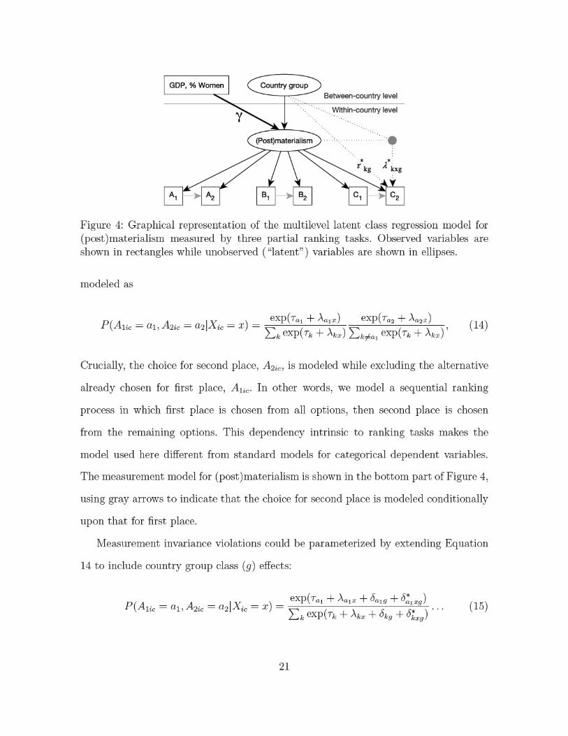
The base invariance model in Equation 14 can be seen as fixing the direct main effects

δkg = 0 and direct interaction effects δ∗kxg = 0. Figure 4 shows an example for the second

ranking of Set C (C2) as the dotted main effect and interaction effects. In line with

Section 2, we now investigate whether the possible misspecifications in the measurement

invariance model, δkg 6= 0 and δ∗kxg 6= 0, substantially affect the parameters of interest

γmx using EPC-interest for categorical data.

The full measurement invariance model including parameters of interest γmx was

estimated using Latent GOLD 5. Following Moors and Vermunt (2007), we select three

classes for both the latent “(post)materialism” variable and the country group class

variable, T = S = 3. For BIC values and the rationale behind these choices, please see

Appendix C. Since class selection is not the focus of this example analysis, we will not

discuss it here further.

After estimating the full invariance model, we calculated the EPC-interest for the

δ and δ∗ parameters, of which our three-class model has four: two for each of the

two independent variables. Measurement invariance violations can potentially take the

form of 6 direct main effects (δjkg) and 12 direct interaction effects (δ∗jkxg) for each

of the three ranking tasks, totaling 54 possible misspecifications in the full invariance

model. These misspecifications are strongly correlated and should not be considered

separately. Rather, we consider the probable impact of freeing the direct main effects

for each ranking task separately and of freeing the direct interactions for each ranking

task separately. Thus, rather than consider the direct and interaction effects for each

of the 48 countries on each of the three unique categories of each of the three ranking

tasks, making for 5076 potential EPC-interest values, we evaluate direct effects of the

country group random effect and consider their impact jointly for strongly correlated

misspecifications, reducing the problem to 24 EPC-interest values of interest.

Table 3 shows these 24 EPC-interest values together with the parameter estimates

22

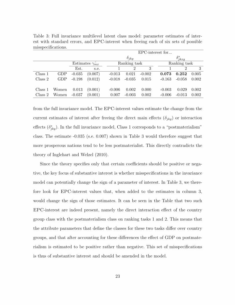
Table 3: Full invariance multilevel latent class model: parameter estimates of inter-est with standard errors, and EPC-interest when freeing each of six sets of possiblemisspecifications.

EPC-interest for...δjkg δ∗jkxg

Estimates ˆγmx Ranking task Ranking taskEst. s.e. 1 2 3 1 2 3

Class 1 GDP -0.035 (0.007) -0.013 0.021 -0.002 0.073 0.252 0.005Class 2 GDP -0.198 (0.012) -0.018 -0.035 0.015 -0.163 -0.058 0.002

Class 1 Women 0.013 (0.001) -0.006 0.002 0.000 -0.003 0.029 0.002Class 2 Women -0.037 (0.001) 0.007 -0.003 0.002 -0.006 -0.013 0.002

from the full invariance model. The EPC-interest values estimate the change from the

current estimates of interest after freeing the direct main effects (δjkg) or interaction

effects (δ∗jkg). In the full invariance model, Class 1 corresponds to a “postmaterialism”

class. The estimate -0.035 (s.e. 0.007) shown in Table 3 would therefore suggest that

more prosperous nations tend to be less postmaterialist. This directly contradicts the

theory of Inglehart and Welzel (2010).

Since the theory specifies only that certain coefficients should be positive or nega-

tive, the key focus of substantive interest is whether misspecifications in the invariance

model can potentially change the sign of a parameter of interest. In Table 3, we there-

fore look for EPC-interest values that, when added to the estimates in column 3,

would change the sign of those estimates. It can be seen in the Table that two such

EPC-interest are indeed present, namely the direct interaction effect of the country

group class with the postmaterialism class on ranking tasks 1 and 2. This means that

the attribute parameters that define the classes for these two tasks differ over country

groups, and that after accounting for these differences the effect of GDP on postmate-

rialism is estimated to be positive rather than negative. This set of misspecifications

is thus of substantive interest and should be amended in the model.

23

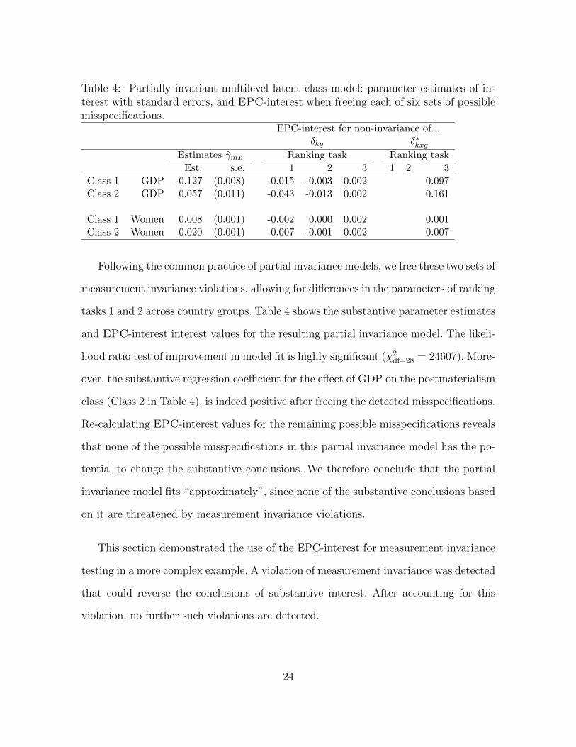
Table 4: Partially invariant multilevel latent class model: parameter estimates of in-terest with standard errors, and EPC-interest when freeing each of six sets of possiblemisspecifications.

EPC-interest for non-invariance of...δkg δ∗kxg

Estimates γmx Ranking task Ranking taskEst. s.e. 1 2 3 1 2 3

Class 1 GDP -0.127 (0.008) -0.015 -0.003 0.002 0.097Class 2 GDP 0.057 (0.011) -0.043 -0.013 0.002 0.161

Class 1 Women 0.008 (0.001) -0.002 0.000 0.002 0.001Class 2 Women 0.020 (0.001) -0.007 -0.001 0.002 0.007

Following the common practice of partial invariance models, we free these two sets of

measurement invariance violations, allowing for differences in the parameters of ranking

tasks 1 and 2 across country groups. Table 4 shows the substantive parameter estimates

and EPC-interest interest values for the resulting partial invariance model. The likeli-

hood ratio test of improvement in model fit is highly significant (χ2df=28 = 24607). More-

over, the substantive regression coefficient for the effect of GDP on the postmaterialism

class (Class 2 in Table 4), is indeed positive after freeing the detected misspecifications.

Re-calculating EPC-interest values for the remaining possible misspecifications reveals

that none of the possible misspecifications in this partial invariance model has the po-

tential to change the substantive conclusions. We therefore conclude that the partial

invariance model fits “approximately”, since none of the substantive conclusions based

on it are threatened by measurement invariance violations.

This section demonstrated the use of the EPC-interest for measurement invariance

testing in a more complex example. A violation of measurement invariance was detected

that could reverse the conclusions of substantive interest. After accounting for this

violation, no further such violations are detected.

24

5. DISCUSSION AND CONCLUSION

Whenever groups are compared, measurement invariance is a concern. Particularly,

it should be verified that substantive conclusions of interest are uncontaminated by

possible cross-group differences in measurement. The “expected parameter change in

the parameter of interest” or EPC-interest, a measure introduced by Oberski (2014)

for this purpose in the context of linear structural equation models, was extended in

this paper to categorical observed and latent variables as well as rankings and other

types of data often encountered in the social sciences.

The EPC-interest for categorical data is an approximation of the change in the pa-

rameters of substantive interest that we can expect to observe if a particular violation

of measurement invariance were freed. A small simulation study showed that this ap-

proximation works well when the misspecification is moderate, and overestimates the

bias somewhat when it is extreme. In this case, EPC-interest still indicates the most

important violations of measurement invariance but the researcher may wish to verify

that the expected parameter change is close to the actually observed change.

Two example applications of categorical data latent variable models demonstrated

the utility of the EPC-interest. The first application formulated a simple IRT-type

“ideal point” model for US senators’ votes, modeling their latent ideology as a func-

tion of party membership to estimate polarization in the 90th US Senate. After fitting

the full invariance model, EPC-interest detected one violation of measurement invari-

ance that substantially reduced the estimated polarization and made the ideal point

estimates for some Republican senators considerably more liberal. The second exam-

ple application looked at the relationship between latent (post)materialism on the one

hand and, on the other, log-GDP per capita and the percentage of women in parlia-

ment using data from 67,568 respondents in 48 countries. A violation of measurement

25

invariance existed that, when unaccounted for, could reverse substantive conclusions.

The EPC-interest allowed us to detect this problem and account for those violations

of assumptions that were indeed influential on the substantive conclusions of interest.

The reader might raise the issue of whether it is appropriate to free violations of

measurement invariance when these are encountered7. While this approach has long

been standard practice in both the “partial invariance” literature (Byrne, Shavelson

and Muthen, 1989) and the DIF literature (Holland and Wainer, 1993), there are

indeed situations in which it can be misleading. In particular, freeing violations can

be misleading when this leads to an alternative model in which freeing such violations

for the other indicators is no longer identifiable. An example is a model with only

one invariance restriction so that the alternative model is simply the model with only

a priori reference indicators. In such cases the choice of indicator for which to free

the parameters (i.e. the choice of reference indicator) cannot be determined based

on model fit, and will often lead to opposite changes in the parameters of interest

(Hancock, Stapleton and Arnold-Berkovits, 2009). The EPC-interest can then still be

used to investigate whether the conclusions are robust to violations of the assumptions.

When they are not, however, there is no empirical basis on which to select a model. In

other situations such as in the example applications, however, the alternative model

still imposes testable restrictions on the data. It then seems reasonable to proceed by

freeing some restrictions while retaining others as is the common practice.

REFERENCES

Arel-Bundock, Vincent. 2013. WDI: World Development Indicators (World Bank). R

package version 2.4.

7We thank an anonymous reviewer for bringing this to our attention.

26

URL: http://CRAN.R-project.org/package=WDI

Benjamini, Yoav and Yosef Hochberg. 1995. “Controlling the false discovery rate: a

practical and powerful approach to multiple testing.” Journal of the Royal Statistical

Society. Series B (Methodological) 57:289–300.

Bentler, P.M. and C.P. Chou. 1993. “Some new covariance structure model improve-

ment statistics.” In Testing structural equation models, ed. K.G. Joreskog and J.

Scott Long. Sage focus editions Sage Publications pp. 235–235.

Bockenholt, U. 2002. “Comparison and choice: Analyzing discrete preference data

by latent class scaling models.” In Applied latent class analysis, ed. Jacques A.P.

Hagenaars and Allan L. McCutcheon. cambridge, UK: Cambridge University Press

pp. 163–182.

Bollen, Kenneth A. 2002. “Latent variables in psychology and the social sciences.”

Annual review of psychology 53:605–634.

Byrne, B.M., R.J. Shavelson and Bengt Muthen. 1989. “Testing for the equivalence of

factor covariance and mean structures: The issue of partial measurement invariance.”

Psychological Bulletin 105:456.

Chen, F.F. 2007. “Sensitivity of goodness of fit indexes to lack of measurement invari-

ance.” Structural Equation Modeling 14:464–504.

Cheung, G.W. and R.B. Rensvold. 2002. “Evaluating goodness-of-fit indexes for testing

measurement invariance.” Structural Equation Modeling 9:233–255.

Croon, Marcel. 1989. “Latent Class Models for the Analysis of Rankings.” In New

Developments in Psychological Choice Modelling, ed. G. De Soete, H. Feger and

K. C. Klauer. Elsevier Science Publishers pp. 99–121.

27

French, B.F. and W.H. Finch. 2006. “Confirmatory factor analytic procedures for the

determination of measurement invariance.” Structural Equation Modeling 13:378–

402.

Hancock, Gregory R., Laura M. Stapleton and Ilona Arnold-Berkovits. 2009. “The

tenuousness of invariance tests within multisample covariance and mean structure

models.” In Structural Equation Modeling in Educational Research: Concepts and

Applications, ed. T. Teo and M.S. Khine. Rotterdam, The Netherlands: Sense Pub-

lishers pp. 137–174.

Holland, Paul W and Howard Wainer. 1993. Differential item functioning. Hillsdale:

Lawrence Erlbaum Associates.

Hu, L. and P.M. Bentler. 1998. “Fit indices in covariance structure modeling: Sensitivity

to underparameterized model misspecification.” Psychological methods 3:424.

Inglehart, Ronald. 1977. The silent revolution. Princeton: Princeton University Press.

Inglehart, Ronald. 1981. “Post-materialism in an environment of insecurity.” The

American Political Science Review 75:880–900.

Inglehart, Ronald and Christian Welzel. 2010. “Changing mass priorities: The link

between modernization and democracy.” Perspectives on Politics 8:551–567.

Inglehart, Ronald, Pippa Norris and Christian Welzel. 2002. “Gender equality and

democracy.” Comparative Sociology 1:321–345.

Kankaras, Milos, Guy Moors and Jeroen K Vermunt. 2010. “Testing for measurement

invariance with latent class analysis.” In Cross-cultural analysis: Methods and appli-

cations, ed. Eldad Davidov, Peter Schmidt and Jaak Billiet. New York: Taylor &

Francis pp. 359–384.

28

Luce, R. Duncan. 1959. Individual Choice Behavior: a Theoretical Analysis. New York:

John Wiley and Sons.

Lukociene, Olga, Roberta Varriale and Jeroen K Vermunt. 2010. “The simultaneous

decision(s) about the number of lower-and higher-level classes in multilevel latent

class analysis.” Sociological Methodology 40:247–283.

Magnus, J.R. and A.L. Vasnev. 2007. “Local sensitivity and diagnostic tests.” The

Econometrics Journal 10:166–192.

Magnus, J.R. and H. Neudecker. 2007. Matrix Differential Calculus with Applications

in Statistics and Econometrics, Third Edition. New York: John Wiley & Sons.

McCutcheon, Allan L. 1985. “A latent class analysis of tolerance for nonconformity in

the American public.” Public Opinion Quarterly 49:474–488.

Mellenbergh, G.J. 1989. “Item bias and item response theory.” International Journal

of Educational Research 13:127–143.

Meredith, W. 1993. “Measurement invariance, factor analysis and factorial invariance.”

Psychometrika 58:525–543.

Moors, Guy and Jeroen Vermunt. 2007. “Heterogeneity in post-materialist value pri-

orities. Evidence from a latent class discrete choice approach.” European Sociological

Review 23:631–648.

Muthen, Bengt and Tihomir Asparouhov. 2012. “Bayesian structural equation mod-

eling: a more flexible representation of substantive theory.” Psychological methods

17:313.

29

Muthen, Bengt and Tihomir Asparouhov. 2014. “IRT Studies of Many Groups: The

Alignment Method.” Mplus Webnote Version 2014-04-29.

URL: http://www.statmodel.com/download/IRTAlignment.pdf

Oberski, D.L. 2014. “Evaluating Sensitivity of Parameters of Interest to Measurement

Invariance in Latent Variable Models.” Political Analysis 22:45–60.

Poole, Keith, Jeffrey Lewis, James Lo and Royce Carroll. 2012. “oc: OC Roll

Call Analysis Software.” R package version 0.93. URL: http://cran. r-project.

org/web/packages/oc/index. html.

Poole, Keith T and Howard Rosenthal. 1985. “A spatial model for legislative roll call

analysis.” American Journal of Political Science.

Poole, Keith T, Jeffrey B Lewis, James Lo and Royce Carroll. 2008. “Scaling roll call

votes with w-nominate in r.” Available at SSRN 1276082.

R Core Team. 2012. R: A Language and Environment for Statistical Computing. Vi-

enna, Austria: R Foundation for Statistical Computing. ISBN 3-900051-07-0.

URL: http://www.R-project.org/

Rabe-Hesketh, Sophia, Anders Skrondal and Andrew Pickles. 2004. “Generalized mul-

tilevel structural equation modeling.” Psychometrika 69:167–190.

Saris, W.E., A. Satorra and D. Sorbom. 1987. “The Detection and Correction of Speci-

fication Errors in Structural Equation Models.” Sociological Methodology 17:105–129.

Saris, W.E., A. Satorra and W.M. Van der Veld. 2009. “Testing structural equation

models or detection of misspecifications?” Structural Equation Modeling 16:561–582.

Satorra, A. 1989. “Alternative Test Criteria in Covariance Structure Analysis: A Uni-

fied Approach.” Psychometrika 54:131–151.

30

Schmitt, N. and G. Kuljanin. 2008. “Measurement invariance: Review of practice and

implications.” Human Resource Management Review 18:210–222.

Skrondal, Anders and Sofia Rabe-Hesketh. 2004. Generalized latent variable modeling

: multilevel, longitudinal, and structural equation models. Interdisciplinary statistics

series Boca Raton, FL: Chapman & Hall/CRC.

Sorbom, D. 1989. “Model modification.” Psychometrika 54:371–384.

Steenkamp, JBEM and H. Baumgartner. 1998. “Assessing measurement invariance in

cross-national consumer research.” Journal of Consumer Research 25:78–107.

Van De Schoot, Rens, Anouck Kluytmans, Lars Tummers, Peter Lugtig, Joop Hox and

Bengt Muthen. 2013. “Facing off with Scylla and Charybdis: a comparison of scalar,

partial, and the novel possibility of approximate measurement invariance.” Frontiers

in Psychology 4:770.

Vandenberg, R.J. and C.E. Lance. 2000. “A review and synthesis of the measurement

invariance literature: Suggestions, practices, and recommendations for organizational

research.” Organizational Research Methods 3:4–70.

Vermunt, J. K and J. Magidson. 2004. “Factor analysis with categorical indicators: A

comparison between traditional and latent class approaches.” In New developments

in categorical data analysis for the social and behavioral sciences, ed. L. Andries van

der Ark, Marcel A. Croon and Klaas Sijtsma. Mahwah: Erblaum pp. 41–63.

Vermunt, J. K and J. Magidson. 2013. Technical guide for Latent GOLD 5.0: Basic

and advanced. Belmont, MA: Statistical Innovations Inc.

31

A. COUNTRIES INCLUDED IN THE STUDY

ISO3 code Country name ISO3 code Country nameDZA Algeria MAR MoroccoARM Armenia NLD Netherlands, TheAUS Australia NZL New ZealandAZE Azerbaijan NGA NigeriaBLR Belarus PAK PakistanCHL Chile PER PeruCHN China PHL PhilippinesCOL Colombia POL PolandCYP Cyprus QAT QatarECU Ecuador RUS Russian FederationEGY Egypt RWA RwandaEST Estonia SGP SingaporeDEU Germany SVN SloveniaGHA Ghana ESP SpainIRQ Iraq SWE SwedenJPN Japan TTO Trinidad and TobagoJOR Jordan TUN TunisiaKAZ Kazakhstan TUR TurkeyKOR Korea, Republic of UKR UkraineKGZ Kyrgyzstan USA United StatesLBN Lebanon URY UruguayLBY Libya UZB UzbekistaMYS Malaysia YEM YemenMEX Mexico ZWE Zimbabwe

32

B. LATENT GOLD CHOICE INPUT FOR THE FULL INVARIANCE MODEL

The input below fits the full invariance model described in the paper, setting the

possible violations of invariance to zero (0). The option “score test” in the output

section (only available in Latent GOLD or Latent GOLD Choice ≥ 5) is then used

to obtain the EPC-interest values. Output and data for this example can be obtained

from the online appendix at http://.

options

maxthreads=all;

algorithm

tolerance=1e-008 emtolerance=0.01

emiterations=450 nriterations=70 ;

startvalues

seed=0 sets=30 tolerance=1e-005 iterations=50;

bayes

categorical=0 variances=0 latent=0 poisson=0;

missing excludeall;

// NOTE: The option "scoretest" for output is used to obtain

// the EPC-interest. This will also produce the score test ("MI")

// and EPC-self for the measurement invariance restriction

output

parameters=effect betaopts=wl standarderrors profile

probmeans=posterior

frequencies bivariateresiduals estimatedvalues=regression

predictionstatistics setprofile setprobmeans

iterationdetails scoretest ;

// There are several ways of modeling ranking data using LG or LGChoice.

// The most computationally efficient is to use the so-called "3-file"

// setup in LGChoice employed here (see LGChoice manual).

choice = 3

alternatives ’inglehart_wvs6_long.alt’ quote = single

id=alt

choicesets ’inglehart_wvs6_long.set’ quote = single

33

id=set;

variables

groupid country;

caseid id;

choicesetid set ;

dependent value ranking;

independent NY_GDP_PCAP_CD, SG_GEN_PARL_ZS;

attribute int1 nominal, int2 nominal, int3 nominal;

latent

GClass group nominal 3,

Class nominal 3;

equations

// Group class intercept

GClass <- 1 ;

// Parameters of interest are logistic regression coefficients of

// NY_GDP_PCAP_CD and SG_GEN_PARL_ZS.

Class <- 1 + GClass + NY_GDP_PCAP_CD + SG_GEN_PARL_ZS;

// Below, sets of possible violations of measurement invariance have been

// explicitly restricted to equal zero using "(0)". This will

// produce EPC-interest, EPC-self, and Score test output.

value <- int1 + int2 + int3 +

int1 Class + int2 Class + int3 Class +

(0) int1 GClass + (0) int2 GClass + (0) int3 GClass +

(0) int1 Class GClass +

(0) int2 Class GClass +

(0) int3 Class GClass ;

34

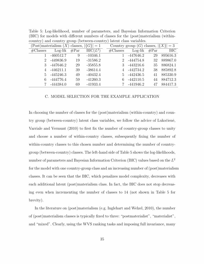
Table 5: Log-likelihood, number of parameters, and Bayesian Information Criterion(BIC) for models with different numbers of classes for the (post)materialism (within-country) and country group (between-country) latent class variables.(Post)materialism (X) classes, |{G}| = 1 Country group (G) classes, |{X}| = 3#Classes Log-lik #Par BIC(L2) #Classes Log-lik #Par BIC

1 -460512.7 9 -10346.1 1 -447646.2 29 895616.32 -449836.9 19 -31586.2 2 -444754.8 32 889867.03 -447646.2 29 -35855.8 3 -443216.6 35 886824.14 -446211.1 39 -38614.4 4 -442734.2 38 885892.85 -445246.3 49 -40432.4 5 -442436.5 41 885330.96 -444776.4 59 -41260.3 6 -442110.5 44 884712.37 -444384.0 69 -41933.4 7 -441946.2 47 884417.3

C. MODEL SELECTION FOR THE EXAMPLE APPLICATION

In choosing the number of classes for the (post)materialism (within-country) and coun-

try group (between-country) latent class variables, we follow the advice of Lukociene,

Varriale and Vermunt (2010) to first fix the number of country-group classes to unity

and choose a number of within-country classes, subsequently fixing the number of

within-country classes to this chosen number and determining the number of country-

group (between-country) classes. The left-hand side of Table 5 shows the log-likelihoods,

number of parameters and Bayesian Information Criterion (BIC) values based on the L2

for the model with one country-group class and an increasing number of (post)materialism

classes. It can be seen that the BIC, which penalizes model complexity, decreases with

each additional latent (post)materialism class. In fact, the BIC does not stop decreas-

ing even when incrementing the number of classes to 14 (not shown in Table 5 for

brevity).

In the literature on (post)materialism (e.g. Inglehart and Welzel, 2010), the number

of (post)materialism classes is typically fixed to three: “postmaterialist”, “materialist”,

and “mixed”. Clearly, using the WVS ranking tasks and imposing full invariance, many

35

more qualitative (post)materialism classes can be distinguished than the traditional

three classes. This corresponds to findings by Moors and Vermunt (2007); however,

these authors also argued that “one can safely interpret the results (...) if adding an-

other class does not result in important changes of the latent class weights for the other

classes” (p. 637). While this is a somewhat subjective criterion, the three-class solution

found in the data does correspond to the theoretical “postmaterialist”, “materialist”,

and “mixed” classes, whose parameters appear to change little in the models with a

greater number of classes. Moreover, the greatest reduction in BIC seen in Table 5

takes place when moving from a one-class to a two-class model, with relatively small

improvements after three or more classes. We therefore follow the theoretical literature

in selecting the three-class model.

While selecting the number of country-group classes, we find that the BIC improves

little after three classes (right-hand side of Table 5), so that our initial full invariance

model has three (post)materialism (within-country) and three country group (between-

country) classes.

D. WVS RANKING DATA MODEL ESTIMATES

Table 6 shows the sizes of the three (post)materialism classes (third row) as well as

the “attribute parameters”, i.e. each class’s average log-utility. Thus, when reading

each row horizontally, the class with the highest log-utility represents respondents who

value that object highest. For example, priorities A.1, A.2, B.1, B.3, and C1 have the

highest log-utilities in Class 1. Since all of these priorities are “materialist” (labeled

“M” in Table 6), we also labeled Class 1 “materialist”. A caveat with this label is

that the materialist priorities that are most strongly related to this class also happen

to be the first item in each set, so that a primacy effect may play a role here as

36

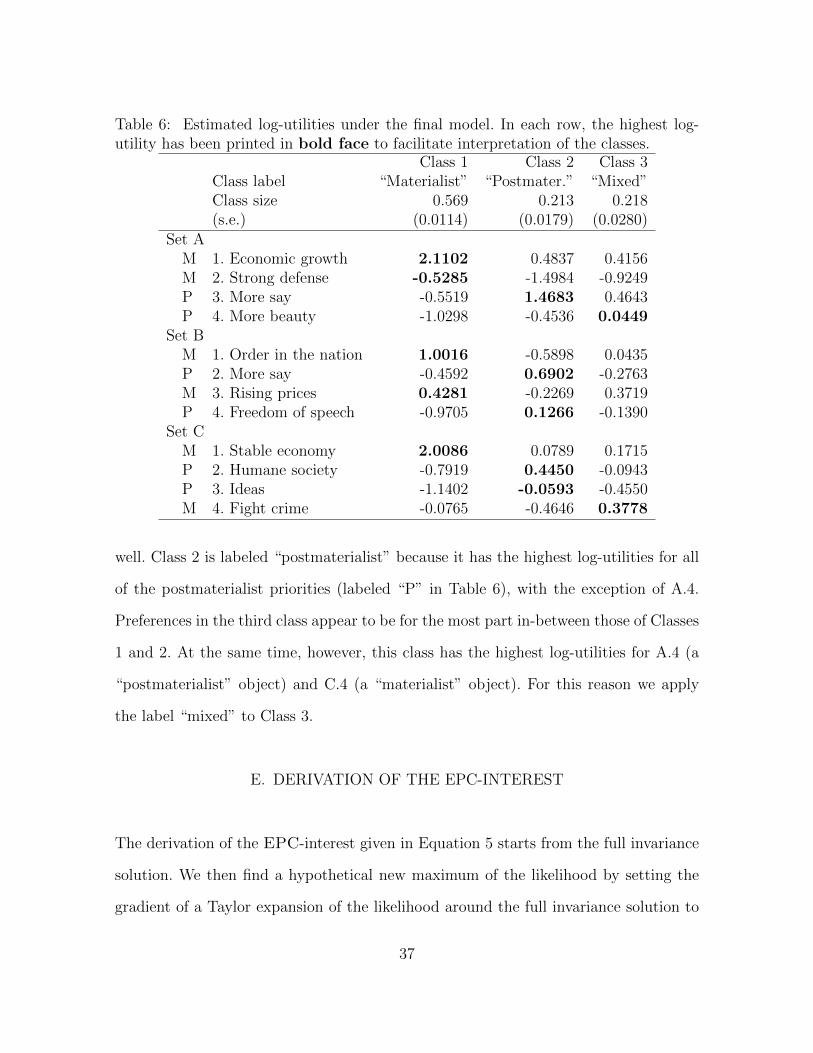
Table 6: Estimated log-utilities under the final model. In each row, the highest log-utility has been printed in bold face to facilitate interpretation of the classes.

Class 1 Class 2 Class 3Class label “Materialist” “Postmater.” “Mixed”Class size 0.569 0.213 0.218(s.e.) (0.0114) (0.0179) (0.0280)

Set AM 1. Economic growth 2.1102 0.4837 0.4156M 2. Strong defense -0.5285 -1.4984 -0.9249P 3. More say -0.5519 1.4683 0.4643P 4. More beauty -1.0298 -0.4536 0.0449

Set BM 1. Order in the nation 1.0016 -0.5898 0.0435P 2. More say -0.4592 0.6902 -0.2763M 3. Rising prices 0.4281 -0.2269 0.3719P 4. Freedom of speech -0.9705 0.1266 -0.1390

Set CM 1. Stable economy 2.0086 0.0789 0.1715P 2. Humane society -0.7919 0.4450 -0.0943P 3. Ideas -1.1402 -0.0593 -0.4550M 4. Fight crime -0.0765 -0.4646 0.3778

well. Class 2 is labeled “postmaterialist” because it has the highest log-utilities for all

of the postmaterialist priorities (labeled “P” in Table 6), with the exception of A.4.

Preferences in the third class appear to be for the most part in-between those of Classes

1 and 2. At the same time, however, this class has the highest log-utilities for A.4 (a

“postmaterialist” object) and C.4 (a “materialist” object). For this reason we apply

the label “mixed” to Class 3.

E. DERIVATION OF THE EPC-INTEREST

The derivation of the EPC-interest given in Equation 5 starts from the full invariance

solution. We then find a hypothetical new maximum of the likelihood by setting the

gradient of a Taylor expansion of the likelihood around the full invariance solution to

37

zero:

∂L(θ,ψ)

∂ϑ= 0 =

∂L(θ,ψ)∂θ|θ=θ

∂L(θ,ψ)∂ψ|θ=θ

+

Hθθ Hψθ

Hψθ Hψψ

θ − θ

ψ − ψ

+O(δ′δ). (16)

A similar device was used to derive the so-called “modification index” or “score test”

for the significance of the hypothesis ψ = 0 by Sorbom (1989, p. 373). Equation

5 follows directly by noting that (∂L(θ,ψ)/∂θ)|θ=θ = 0 and applying the standard

linear algebra result on the inverse of a partitioned matrix(H−1)

θψ= −H

−1θθ HθψD

−1

(e.g. Magnus and Neudecker, 2007, p. 12).

38