Evaluating EOF modes against a stochastic null...

Evaluating EOF modes against a stochastic null hypothesis

Dietmar Dommenget

Received: 19 April 2006 /Accepted: 15 September 2006 / Published online: 18 October 2006! Springer-Verlag 2006

Abstract In this paper it is suggested that a stochasticisotropic diffusive process, representing a spatial firstorder auto regressive process (AR(1)-process), can beused as a null hypothesis for the spatial structure ofclimate variability. By comparing the leading empiricalorthogonal functions (EOFs) of a fitted null hypothesiswith EOF modes of an observed data set, inferencesabout the nature of the observed modes can be made.The concept and procedure of fitting the null hypoth-esis to the observed EOFs is in analogy to time anal-ysis, where an AR(1)-process is fitted to the statistics ofthe time series in order to evaluate the nature of thetime scale behavior of the time series. The formulationof a stochastic null hypothesis allows one to defineteleconnection patterns as those modes that are mostdistinguished from the stochastic null hypothesis. Themethod is applied to several artificial and real data setsincluding the sea surface temperature of the tropicalPacific and Indian Ocean and the Northern Hemi-sphere wintertime and tropical sea level pressure.

1 Introduction

One of the outstanding features of natural climatevariability is that the variability is organized in specificspatial patterns. The El Nino Southern Oscillation(ENSO) mode is such an example. The accuratedescription of the spatial patterns associated to the

modes is therefore an important issue in climateresearch.

Principal component analysis, also known as theempirical functions (EOFs) technique, is the mostwidely used method to identify these patterns. Often asingle EOF mode is analyzed, assuming that this modereflects a specific mode of climate variability with awell defined underlying physical mechanism.

The literature about EOF analysis, its statisticalcharacteristics and alternative methods is vast andnearly intractable (an overview on EOF analysis isgiven in von Storch and Zwiers 1999; Jolliffe 2002 andreferences therein). Some important measures are gi-ven about the statistical uncertainties of EOF eigen-values and patterns due to sampling limitations (Northet al. 1982; Overland and Preisendorfer 1982). Moreimportant in the context of the interpretation of thestatistical modes as reflections of underlying physicalmechanism are studies focusing on the characteristicsof EOF or other statistical modes of simple stochasticmodels, which may give some insight into the struc-tures of the statistical modes as they may appear inobserved physical systems (North 1984; Navarra 1993;Metz 1994; Gerber and Vallis 2005 and many others).North (1984) finds that the EOFs of some simple sto-chastic models driven by spatially white noise coincidewith the eigen modes of the dynamic operator of thesystem. Navarra (1993), Metz (1994), Gerber andVallis (2005) analyzed the atmospheric variability insimplified linearized models and found that the ob-served structures of meridional dipole variability canbe explained by these simplified models.

Much of the discussion of the EOF-analysis is aboutits capability of presenting modes that reflect under-lying physics. In general these discussions follow the

D. Dommenget (&)Leibniz-Institut fur Meereswissenschaften,Dusternbrooker Weg 20, 24105 Kiel, Germanye-mail: [email protected]

123

Clim Dyn (2007) 28:517–531

DOI 10.1007/s00382-006-0195-8

concept of comparing the EOF-analysis with alterna-tive definitions of statistical modes in order to point outwhich method works best (Richman 1986; Brethertonet al. 1992; van den Dool 2000; Aires 2002 and manyothers).

In Dommenget and Latif (2002a) three very simplemodes of variability are used to construct a simpleartificial example, in which the resulting EOF modeshave very little in common with the three modes ofvariability used to create the multivariate problem,thus indicating that EOF modes do not necessarilyreflect physical modes of a system. Although, thiswork only discusses the limitation of EOFs, theconclusions hold essentially for all statistical methodsof defining modes of variability. The dilemma is thatwe like to use the concept of climate modes tounderstand climate variability, while the EOF-analy-sis or alternative statistical methods, which we use todefine these, are pure mathematical concepts whichwill not necessarily detect the physical modes. Theproblem is to some degree due to the fact that thestatistical modes are discussed without having a nullhypothesis of how the statistical modes would looklike if no outstanding climate modes exist. To eval-uate the physical relevance of statistical modes it maytherefore be helpful to formulate a null hypothesisfor the statistical modes against which the observedmodes can be compared.

Calahan et al. (1996) used a stochastic model withspatial correlation to compare the EOF-eigenvalues ofrainfall variability over North America against, whichessentially represents a spatial auto-regressive processof the first order. This approach is very similar to thenull hypothesis used in analysis of time series. HereHasselmann (1976) introduced the stochastic climatemodel as the null hypothesis for the time evolution ofclimate variables, which assumes, in its simplest form,an auto-regressive process of the first order.

In this paper it is illustrated how the formulationof a null hypothesis for the spatial structure ofclimate variability can help to evaluate the physicalnature of EOF or other statistical modes and subse-quently helps to identify outstanding patterns ofclimate variability.

The paper is organized as follows: In Sect. 2 a defi-nition of climate modes and the concept of testing astochastic null hypothesis are discussed. In Sect. 3 anull hypothesis for the spatial variability of climatevariables is formulated. The procedure of how toevaluate EOFs against a stochastic null hypothesis isdescribed in Sect. 4. The concept is applied to severalartificial and real data sets in Sect. 5. The paper con-cludes with a discussion in Sect. 6.

2 Concepts

It is helpful to first discuss how climate modes couldbe defined and how limited such definitions may be.It is also instructive to illustrate how the conceptof testing a stochastic null hypothesis is performed intime series analysis, which will be a guide for thesubsequent analysis of the spatial structures of climatevariables.

2.1 The null hypothesis in time series analysis

It is common in time series to evaluate the spectra oftime series against an first order auto-regressive pro-cess (AR(1)-process), which goes back to the stochasticclimate model of Hasselmann (1976). In its simplestform, Hasselmann’s model is an AR(1)-process, whichis defined by the following differential equation fortime evolution of any physical variable F:

d

dtU ! cdamp " U# f $1%

with cdamp < 0 being a constant damping and f whitenoise. The auto-correlation function in time, c(s), of Fis:

c$s% ! e&s=t0 $2%

with the time lag s and the e-folding time t0 = 1/cdamp.One can derive the analytical form of the spectraldistribution of the null hypothesis of F from Eq. 2. Intime series analysis, this null hypothesis is often used toevaluate the temporal behavior of F, by simply com-paring the spectrum of F with that of a fitted AR(1)-process. The parameters of the fitted AR(1)-processare derived from the auto covariance function of F(e.g. Reynolds 1978; Dommenget and Latif 2002b).

In the case of the El Nino SST time series, for in-stance, the spectrum shows some characteristic en-hanced variance (peak) in the interannual frequencyrange, which is usually interpreted as an indication forthe oscillating nature of El Nino SST. The spectrum ofthe midlatitudes SST time series shows no peak, but adifferent overall slope of the spectrum, which indicatesdeviations from the AR(1)-process null hypothesis(Dommenget and Latif 2002b).

2.2 Definitions of teleconnection/climate modesand their limitations

The way EOFs modes are discussed in most statisticalanalyses (e.g. Dommenget and Latif 2002a and refer-

518 D. Dommenget: Evaluating EOF modes against a stochastic null hypothesis

123

ences therein) is based on a factor analysis approach, aspointed out by Jolliffe (2003). It is implicitly assumedthat the multivariate data X is a result of the timeevolution of a set of K fixed factors, pi, (often calledteleconnections, modes or patterns), and some residualunstructured noise n.

X$t% ! W$t%P# n$t% $3%

P is a matrix of factor loadings pi, where each pi isinterpreted as a coherent spatial pattern (teleconnec-tion). These patterns are the dominating influence forX (for details on factor analysis see textbook by Jolliffe2002). The time evolution of P is given by a matrix oftime series Y.

The idea is to assume that the high-dimensionalsystem can be approximated by a low-order state spacemodel, with the number of modes, K, much smallerthan the dimension of X (von Storch and Zwiers 1999,Sect. 15.5). The patterns P in this approach are areflection of the underlying low-order physical model.This approach, however, depends strongly on how thepatterns P are estimated. In the recent literature itseems a popular approach to associate the leadingEOFs or other statistical modes with the leading tele-connections (e.g. Thompson and Wallace 1998 or Sajiet al. 1999). It is, however, important to note that it isin general unclear if any teleconnections exist in thedata set and how they can be estimated (e.g. Jolliffe2002, Sect. 7 and Dommenget and Latif 2002a).Dommenget and Latif (2002a) argue that most likelyneither EOF nor VARIMAX will find the leadingteleconnection factors in climate data sets. The inher-ent problem in this approach is that a criteria oralgorithm needs to be formulated by which theempirical patterns P are chosen. Thus the resultingmodes may in many cases be a reflection of the sta-tistical method used, but are not a good representationof the underlying physical processes.

An alternative method, which avoids to formulateany criteria for the structure of teleconnection modes,is to formulate a null hypothesis for the structure ofspatial variability, which can be regarded as a modelfor the noise. Any pattern that is very distinct from thepatterns of the null hypothesis is a good starting pointfor the estimation of teleconnection modes. This con-cept is similar to the time series analysis, in which thetime scale behavior of El Nino, for instance, is sim-plified into a distinct oscillation mode on interannualtime scales and a background red noise. In analogy theteleconnection modes are defined as the modes thatstick out of the background noise, as define by the nullhypothesis.

3 A stochastic null hypothesis for the spatial structureof climate variability

The stochastic model of Calahan et al. (1996) isessentially given by the correlation between two spatiallocations of the data field, F:

c$r% ! e&r=d0 $4%

Here r is the distance between the two locations and d0is the decorrelation length. Note that Eq. 4 is theequivalent to Eq. 2. Thus the stochastic model ofCalahan et al. (1996) is an AR(1)-process in the spatialdomain dimension.

The simple physical model in Eq. 1 can be extendedto include diffusion for the relation between twolocations:

d

dtU ! cdamp " U# cdiffuser2U# f $5%

cdiffuse is a diffusion coefficient and f now representsspatial and temporal white noise. In this equation thediffusion is just introduced in a statistical sense. Thisdiffusion model is often refered to as a simple energybalance models of the climate system (see e.g. Northet al. 1981, 1983 and references there in). Leung andNorth (1991) discussed some statistics of this model forthe atmospheric variability of a zonally symmetricplanet. North (1984) finds that the EOFs of this modeldriven by homogenous forcing f (spatially white noisewith the standard deviation of f constant over the do-main) coincide with the eigen modes of the dynamicoperator of the system.

Note that for an isotropic diffusive process (neithercdamp nor cdiffuse are a function of the location) drivenby a homogenous forcing f, the model in Eq. 5 is anAR(1)-process in the spatial domain. We can derivethe covariance matrix of F:

Rij ! rirje&dij=d0 $6%

where ri is the standard deviation of F at point i and dijthe spatial distance between the two points i and j. Ifthe standard deviation field r or d0 exhibit spatialvariations (e.g. ri „ rj for i „ j), than the model inEq. 5 is not a spatial AR(1)-process any more andEq. 6 does not exactly represent the covariance matrixof F. However, Eq. 6 should be a good approximationif the spatial variations of ri and d0 are small. Theeffect of spatial variations of r will be discussed in Sect.5 by means of a realistic example.

An isotropic diffusive process in Eqs. 5 and 6 isthe null hypothesis for the spatial characteristics of a

D. Dommenget: Evaluating EOF modes against a stochastic null hypothesis 519

123

climate variable F. In this formulation, F has noteleconnections other than the exponential decay of itsauto-correlation function. In analogy, the spectrum ofa time series of an AR(1)-process, is not considered tohave a significant time scale (peak in the spectrum)other than a damping time scale.

We can find the EOF modes and eigenvalues of thenull hypothesis numerically. In Fig. 1 the leading EOFmodes of a domain defined by 17 · 11 points withconstant r = 1 and d0 = 4.6 points is shown. The ei-genvalues of the leading EOF modes are also shown inFig. 1.

Based on this example and a few other exampleswith variations in the domain dimensions and d0 (notshown), a few important characteristics of the EOFmodes and eigenvalues of the diffusion null hypothesiscan be formulated as follows:

• The EOF modes are a hierarchy of multi poles,starting with a monopole as EOF-1, followed by adipole, and then by higher order multi poles. Theorder and structure of the multi poles is a result ofthe domain dimensions and the decorrelationlength d0. Note that this kind of structure of theobserved leading EOF modes of most climate datasets is also discussed in Richman (1986), but not inthe context of the simple stochastic model in (5).

• The EOF-1 peaks in the center of the domain,because the center point is the point which is in

average closest to all other points and has thereforea larger covariance with all other points. Note thatr and d0 are identical for all points, so that thestatistics of all points of the domain are identical.The EOF-1 mode is therefore only a reflection ofthe domain geometry. It simply reflects that there isno structure in the variability other than exponen-tial decay of covariance with distance.

• None of the EOF modes represent teleconnections(factors), since no teleconnections exist in thissimple model. In the simple model of an spatialAR(1)-process the spatial variability is a continuousspectrum of spatial patterns, where no spatialpattern is dominating over the other patterns. TheEOF modes should be interpreted as a reflection ofdifferent spatial scales. In analogy, the spectralcoefficients of a continuous spectrum of an AR(1)-process are a reflection of the different time scales,but not a representation of an oscillating behavior.The domain wide monopole of the leading EOF-1represents the largest spatial scale of variability inthe domain, which in an AR(1)-process has thelargest variance. EOF-2 and EOF-4, for instance,should be interpreted as spatial variability along thex-axis with a spatial length scale of about 1/2 of thedomain size along the x-axis. They do not representan anti correlation between the centers. The sameholds for all other EOF modes.

1 3 5 7 9 11 13 15 17 190

5

10

15

20

25

expl

aine

d va

rianc

e [%

]

eigenvalue number

Eigenvalues of a diffusive stochastic process

Fig. 1 The leading EOF modes (left panels) and eigenvalues (right panel) of a spatial AR(1)-process in a 17 · 11 points domain


123

• The decrease of the eigenvalues to higher orderEOFs is only a function of the domain size and thedecorrelation length d0. None of the 20 leadingeigenvalues is degenerated (equal to another eigen-value), reflecting the different length of the domainalong the x- and y-axis. Note that in this examplethe number of points in each direction was chosenas a prime number to avoid degenerated eigen-values, which in real domains, such as ocean basins,would not occur. Note also that the numericalprecision of the EOF analysis in this example ismuch better than the line (dot) thickness in Fig. 1.

An important quantity that quantifies the degree ofcomplexity in the domains spatial variability is theeffective spatial number of degrees of freedom Neff

(Bretherton et al. 1999). It essentially estimates theeffective dimension of the multivariate variability:

Neff !1Pe2i

; withX

ei ! 1 $7%

with ei the eigenvalues as derived from the EOFanalysis. The number Neff corresponds to the numberof independent spatial modes. It also quantifies thedecrease of the eigenvalues and is a monotonic func-tion of the decorrelation length d0. It can therefore alsobe used as an estimate for the decorrelation length.

4 Evaluating EOF-vectors and eigenvalues against astochastic null hypothesis

The stochastic model allows an evaluation of EOFmodes. In many studies only the leading EOF modes ofan observed data set are discussed. Here the focus isoften on the spatial structure of the observed EOFpatterns, which are interpreted as teleconnection pat-terns. It is therefore important to discuss to which de-gree the leading EOF modes are consistent with thesimple null hypothesis or, in a more objective ap-proach, to find those patterns, that are most distin-guished from those of the null hypothesis.

4.1 Fitting an isotropic diffusion process to data

The null hypothesis as formulated in the previoussection can be fitted to any data set by estimating thestandard deviation field r and the average decorrela-tion length d0. Given r and d0 the covariance matrix ofthe null hypothesis in Eq. 6 is defined and the EOFmodes of the null hypothesis can be calculated.

Note that the estimation of d0 can have largeuncertainties in a limited gridded domain (see e.g. von

Storch and Zwiers 1999). However, d0 is a monotonicfunction of the spatial number of degrees of freedom,Neff, which is estimated by the sum of eigenvalues. Theestimation of d0 will usually depend on the correlationof neighboring points, which is a function of the vari-ability on all spatial scales. The estimation of Neff isessentially a function of the leading EOF-modes only,while the small scale variability has little effect on thisquantity. Hence, the agreement between the leadingeigenvalues of the observations and the fitted nullhypothesis appears to be better if the observed Neff isused to estimate the fitted d0 in Eq. 6. An analyticalrelation between Neff and d0 may exist for some simpledomain geometries, such as a sphere for instance.However, it will be difficult to write down an analyticalrelation for complicated geometry and boundary con-ditions and it may therefore be most practical to esti-mate these quantities numerically. Thus, d0 is varieduntil Neff of the fitted null hypothesis agrees with theNeff of the observational data set within the uncertaintyrange of Neff, which should be given by the statisticaluncertainties of the eigenvalues due to sampling errors(North et al. 1982).

4.2 Comparing the observed EOF modes with anull hypothesis

An EOF eigenvector (mode) of an observed data set,~Eobs

i ; and the corresponding eigenvalue eiobs can be

compared to the eigenvectors ~Enullj and eigenvalues ej-

null of a null hypothesis by projecting the eigenvectors~Enull

j onto the eigenvector ~Eobsi :

cij !~Eobs

i~Enull

j

j~Eobsi jj ~Enull

j j$8%

cij is the uncentered pattern correlation coefficientbetween the two EOF-patterns. The variance that themode ~Eobs

i would have under the null hypothesis can beestimated by the linear combination of all eigenvaluesejnull of the null hypothesis using cij:

eobsnulli !XN

j!1

c2ijenullj : $9%

The variance eiobsnull is the expected variance of ~Eobs

i

if the data follows the diffusive process of thenull hypothesis. Note that while the eigenvalues ei

obs

decrease monotonically with higher order numbers, theeiobsnull values does not need to decrease with higherorder number. A pattern that explains a lot of variance


123

in the observations (large eiobs) may explain little var-

iance under the null hypothesis (small eiobsnull values).

4.3 Statistical inferences about the nature of EOFmodes

The uncertainties of the eigenvalues eiobs of the ob-

served data due to sampling errors are given byNorth et al. (1982). When the observed data followsthe null hypothesis we expected the ei

obsnull value tobe within the uncertainties of the eigenvalues ei

obs. Acomparison of the eigenvalue spectrum ei

obs with thespectrum of ei

obsnull allows to quantify the deviationsof the observed data from the null hypothesis, whichcan be the basis for statistical inferences about thenature of EOF modes. The concept is in analogousto the comparison of the spectrum of an observedtime series with the spectrum of the fitted AR(1)-process.

eiobs and ei

obsnull are variances, which tend to be v2-distributed. Statistical inferences about v2-distributedrandom variables are usually obtained on the basis ofthe ratio, ei

obs/eiobsnull, as in time series analysis (e.g.

Reynolds 1978; Dommenget and Latif 2002b). How-ever, as mentioned in Calahan et al. (1996), thestrongest deviations of the ratio, ei

obs/eiobsnull, are found

in the low (higher order) eigenvalues, which are inmost studies of little interest. It therefore may be moreinstructive for large-scale teleconnections to base thestatistical inferences on the difference between ei

obs andeiobsnull. However, the choice of the right test variabledepends on the focus of the analysis.

The method of projecting the null hypothesisonto observed patterns can be used for all kind ofpatterns, like box-averages or more sophisticatedindices. The explained variance of the index com-pared to the explained variance eobsnull could revealwhether the index indeed presents an unexpectedstructure and thus can be used to justify a specificchoice of indices.

5 DEOFs: An estimate of teleconnection modes

If the ~Eobs appear to be different from the nullhypothesis one may be interested in the spatial patternthat maximizes the difference in explained variancebetween the data and the null hypothesis. These arenamed distinct EOFs (DEOFs or ~Dobs% and distinctPCs for the time series (DPCs), respectively. Theleading ~Dobs is defined as the pattern that maximizesthe differences in explained variance Dvar:

Dvar ! Varobs$~Dobs% &Varnull$~Dobs% $10%

where Varobs denotes the variance that the pattern~Dobs explains in the observed data and Varnull denotesthe variance that the pattern ~Dobs explains under thenull hypothesis following (9) The leading ~Dobs can befound by pairwise rotation of the leading EOFs, as it isdone for determining the VARIMAX modes (Kaiser1958), until the maximum of Dvar is found. By iteratingthis procedure we can define a complete set oforthogonal DEOFs, building a complete representa-tion of the data.

The patterns that are most distinguished from thenull hypothesis, the leading DEOFs, are, from a sta-tistical point of view, a good first guess for the tele-connections. They should in general be a good startingpoint for the understanding of the underlying physicalprocesses.

The DEOF have, however, some limitation in theinterpretation, that are similar to those pointed outfor EOFs in Sect. 3. Identifying the DEOFs withcoherent teleconnections depends on the formulationof the null hypothesis. Furthermore, the concept ofteleconnection patterns may not always be helpful inthe understanding of the multivariate data. In somesystems, for instance, the DEOFs are a reflectionanisotropy in the diffusion or advection, which arebetter described by physical process parameter.Coherent teleconnection patterns may not exist insuch systems. The DEOFs focus on the deviationsin the leading (large) eigenvalues, while differencesin the higher order (small) eigenvalues are neglected,which in some systems may be important for theunderstanding of the underlying physical processes(Crommelin and Majda 2004).

The DEOF are defined in an orthogonal system,which, similar to EOFs, maximize some variance cri-teria. Therefore it can be difficult to interpret theDEOFs in systems where many DEOFs explain morevariance than expected under the null hypothesis(see also the discussion of the observed NorthernHemisphere and tropical SLP variability in Sects. 5.5,5.6 and 6).

Note that due to the limited length of the time seriesthe expected value of Dvar is larger then zero, when thedata follows the null hypothesis. For statistical infer-ence about the significance of Dvar of the leadingDEOF we have to estimate the probability distributionfunction (PDF) of Dvar. The simplest way to estimatethe PDF of Dvar of the leading DEOF is by means of abootstrapping approach (see von Storch and Zwiers1999).


123

6 Examples

We start with some artificial examples, in which thetrue nature of the problem is well defined. The twoartificial examples illustrate two different ways inwhich a multivariate data set can differ from a pureisotropic diffusion process. We shall then discuss sev-eral examples of observed climate variability, some ofwhich have led to some controversy in the recent lit-erature. In the discussion of all examples, the nullhypothesis of the climate variability is an isotropicdiffusion process as formulated in Sect. 3 and theparameters are fitted to the data as described in Sect.4.1. The discussion of the observed climate variabilitymodes will be brief and focuses on the new technique.A more detailed physical analysis of the observed cli-mate variability modes may be desirable, but would bebeyond the scope of this paper.

6.1 An isotropic diffusive field with inhomogeneousstandard deviation

The following example is a numerical stochastic reali-zation of Eq. 5, which should be similar in its statisticsto typical monthly mean time series of ocean basinSSTs. The model in Eq. 5 was integrated on a grid with18 · 18 points with a daily time step. The diffusioncoefficient was chosen to produce a decorrelationlength of about 3 points. For the statistical analysis, 30time steps were averaged to build a monthly mean andthe damping cdamp in Eq. 5 was chosen to create a onemonth lag correlation of about 0.6. The resulting timeseries has a length of 1,000 months with about 500degrees of freedom. The standard deviation of thespatially uncorrelated forcing f was increased in tworegions, with one peak in the northeast and one in thesouthwest. The resulting standard deviation of F variesbetween 1.0 and 4.0 (at the peaks) in arbitrary units.The EOF analysis was performed on only the central10 · 10 domain to avoid boundary effects.

In Fig. 2a–c, the leading EOFs of the stochasticsimulation are shown. In addition, the leading EOFs ofthe covariance matrix S based on Eq. 6 with parame-ters ri and d0 fitted to the statistics of the simulationare shown for comparison (Fig. 2d–f). The explainedvariance of the EOF modes of the simulation, ei

obs, arecompared with the fitted isotropic diffusion process byprojecting the EOF modes of the null hypothesis ontothe EOF modes of the stochastic simulation as outlinedin Sect. 4 using Eqs. (8) and (9) (see Fig. 2g). Note thatwhile the eigenvalues ei

obs decrease monotonically withhigher order numbers, the variance under the nullhypothesis, ei

obsnull, does not need to decrease with

higher order number, because these are not eigen-values (see section 4.2).

In a first comparison we find that the EOF modesand eigenvalues of the stochastic simulation are ingood agreement with the fitted null hypothesis. If werotate towards the leading vectors ~Dobs; which pointtowards the largest differences, the two leadingmodes (see Fig. 2h, i) reveal some significant struc-tures (no other higher order mode shows any signif-icant differences). These two structures representsome differences in the spatial scale of variabilitynear the two centers of the leading EOF mode. Theyreflect that Eq. 6 is only an approximation if struc-tures in r or d0 exist. In this example the structureintroduced in the standard deviation of the whitenoise forcing f leads to some structure in the standarddeviation of F and it also creates some variations ind0. However, the difference between the stochasticsimulation and the null hypothesis amounts to only4% for the leading mode.

If we repeat the experiment with a homogenousstandard deviation of the forcing f, the significantstructure in the leading vectors ~Dobs is gone (the dif-ference in explained variance is < 2%, decreasing withthe length of the time series).

In summary, the EOF modes and eigenvalues areclose to those of the null hypothesis.

6.2 A diffusive field with a weak teleconnectionpattern

Here the standard deviation of the forcing f is homo-geneous through out the domain. In addition to thespatially and temporally white noise forcing f, a tele-connection forcing pattern p was introduced in Eq. 5leading to the following equation:

d

dtU ! cdamp " U# cdiffuser2U# p " F # f $11%

The spatial pattern of p is shown in Fig. 3a, where F isa white noise time series with a variance of about 12%of the variance of f. The teleconnection forcing patternp is therefore relatively weak. Figure 3b, c highlightsthe correlation between the two centers of the tele-connection forcing pattern by means of box correla-tions, showing only a weak correlation in F betweenthe two centers. For the EOF analysis, the data werenormalized so that each point has unity standarddeviation. As a result the stochastic simulation reflectsa domain which has no structure in the standarddeviation of F, but it has a structure in the covariancematrix forced by a teleconnection pattern.


123

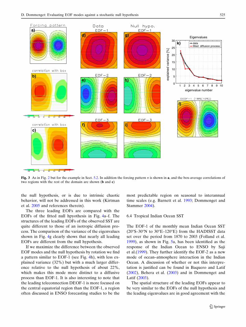
The EOF modes and eigenvalues are shown inFig. 3d–k. The EOF modes are very similar to those ofa purely diffusive process as discussed in Sect. 3, butthe eigenvalue of EOF-2 is larger than expected by adiffusive process. The leading mode of the rotationtowards the largest difference relative to the fittedisotropic diffusion process, DEOF-1, is very similar tothe teleconnection forcing pattern. DEOF-1 explains18% of the total variance, where this pattern wouldonly explain 10% in the fitted AR(1)-process (seeFig. 3l). Thus the residual of about 8% of the totalexplained variance may be associated with a telecon-nection following the spatial structure of DEOF-1.Note that none of the leading VARIMAX modes (notshown) have any similarity to the teleconnection p,

because the structure of the teleconnection forcingpattern (a dipole) does not maximize the VARIMAXcriteria ‘simplicity’.

6.3 Tropical Pacific SST

The first example of observed data is the tropical Pa-cific (from 30"–30"N to 100"E–70"W) monthly meanSST as presented by the HADISST data set from 1870to 2003 (Folland et al. 1999). The ENSO mode in thetropical Pacific is probably the best understood tele-connection mode of natural global climate variabilityand is therefore a good example on which to applythe analysis introduced in this paper. Whether or notthe ENSO mode is stochastically forced, as assumed by

1 2 3 4 5 6 7 8 9 100

5

10

15

20

25

30

35

expl

aine

d va

rianc

e [%

]

eigenvalue number

Eigenvalues

g)d)a)

b)

c) f)

e)

datafitted diffusion process

h) i)

Fig. 2 The leading EOFs of the stochastic simulation (a–c) andthe EOFs of the fitted isotropic diffusion process (d–f) of theexample in Sect. 5.1 are shown. The eigenvalues ei

obs (black line)are compared with the projection of the fitted diffusion processeiobsnull (red line) in g. The shaded envelope around the black lineis the statistical uncertainty of the eigenvalues ei

obs due tosampling errors after North et al.(1982). h and i show the leading

DEOF-1 and DEOF-2. The first percentage value in the headingof the h and i give the explained variance of the DEOF in thestochastic simulation and the second value the explainedvariance of the DEOF under the null hypothesis. All spatialmodes are in arbitrary units. Dashed contours indicate negativevalues


123

the null hypothesis, or is due to intrinsic chaoticbehavior, will not be addressed in this work (Kirtmanet al. 2005 and references therein).

The three leading EOFs are compared with theEOFs of the fitted null hpyothesis in Fig. 4a–f. Thestructures of the leading EOFs of the observed SST arequite different to those of an isotropic diffusion pro-cess. The comparison of the variance of the eigenvaluesshown in Fig. 4g clearly shows that nearly all leadingEOFs are different from the null hypothesis.

If we maximize the difference between the observedEOF modes and the null hypothesis by rotation we finda pattern similar to EOF-1 (see Fig. 4h), with less ex-plained variance (32%) but with a much larger differ-ence relative to the null hypothesis of about 22%,which makes this mode more distinct to a diffusiveprocess than EOF-1. It is also interesting to note thatthe leading teleconnection DEOF-1 is more focused onthe central equatorial region than the EOF-1, a regionoften discussed in ENSO forecasting studies to be the

most predictable region on seasonal to interannualtime scales (e.g. Barnett et al. 1993; Dommenget andStammer 2004).

6.4 Tropical Indian Ocean SST

The EOF-1 of the monthly mean Indian Ocean SST(20"S–30"N to 30"E–120"E) from the HADISST dataset over the period from 1870 to 2003 (Folland et al.1999), as shown in Fig. 5a, has been identified as theresponse of the Indian Ocean to ENSO by Sajiet al.(1999). They further identify the EOF-2 as a newmode of ocean–atmosphere interaction in the IndianOcean. A discussion of whether or not this interpre-tation is justified can be found in Baquero and Latif(2002), Behera et al. (2003) and in Dommenget andLatif (2003).

The spatial structure of the leading EOFs appear tobe very similar to the EOFs of the null hypothesis andthe leading eigenvalues are in good agreement with the

1 2 3 4 5 6 7 8 9 100

5

10

15

20

25

30

expl

aine

d va

rianc

e [%

]

eigenvalue number

Eigenvalues

k)

g)d)a)

b)

c)

e) h)


l)

i)f)

Fig. 3 As in Fig. 2 but for the example in Sect. 5.2. In addition the forcing pattern p is shown in a, and the box-average correlations oftwo regions with the rest of the domain are shown (b and c)


123

variance of the null hypothesis (see Fig. 5a–g). Ittherefore seems that the SST variability of the IndianOcean is consistent with a purely diffusive process. Inparticular, EOF-2, the so called Indian ocean dipolemode, explains less variance than expected from thefitted AR(1)-process.

Although there is no indication for strong deviationsfrom an isotropic diffusion process, a rotation towardsthe leading differences from the null hypothesis wasperformed (see Fig. 5h). However, DEOF-1 explaining32% of the total variance (24% in the null hypothesis)is only slightly different from the null hypothesis.

1 2 3 4 5 6 7 8 9 100

10

20

30

40

50

expl

aine

d va

rianc

e [%

]

eigenvalue number

Eigenvalues

g)

h)f)

e)

d)a)

b)

c)


Fig. 4 As in Fig. 2 but for the tropical Pacific SST as discussed in Sect. 5.3

1 2 3 4 5 6 7 8 9 100

10

20

30

40

50

60ex

plai

ned

varia

nce

[%]

eigenvalue number

Eigenvalues

g)

a) d)

e)

f)c)

c)


h)

Fig. 5 As in Fig. 2 but for the tropical Indian Ocean SST as discussed in Sect. 5.4


123

6.5 Northern hemisphere winter time SLP

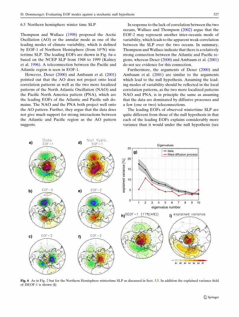
Thompson and Wallace (1998) proposed the ArcticOscillation (AO) or the annular mode as one of theleading modes of climate variability, which is definedby EOF-1 of Northern Hemisphere (from 10"N) win-tertime SLP. The leading EOFs are shown in Fig. 6a–cbased on the NCEP SLP from 1948 to 1999 (Kalneyet al. 1996). A teleconnection between the Pacific andAtlantic region is seen in EOF-1.

However, Deser (2000) and Ambaum et al. (2001)pointed out that the AO does not project onto localcorrelation patterns as well as the two more localizedpatterns of the North Atlantic Oscillation (NAO) andthe Pacific North America pattern (PNA), which arethe leading EOFs of the Atlantic and Pacific sub do-mains. The NAO and the PNA both project well ontothe AO pattern. Further, they argue that the data doesnot give much support for strong interactions betweenthe Atlantic and Pacific region as the AO patternsuggests.

In response to the lack of correlation between the twooceans, Wallace and Thompson (2002) argue that theEOF-2 may represent another inter-oceanic mode ofvariability, which leads to the apparent weak correlationbetween the SLP over the two oceans. In summary,Thompson andWallace indicate that there is a relativelystrong connection between the Atlantic and Pacific re-gions, whereas Deser (2000) and Ambaum et al. (2001)do not see evidence for this connection.

Furthermore, the arguments of Deser (2000) andAmbaum et al. (2001) are similar to the argumentswhich lead to the null hypothesis. Assuming the lead-ing modes of variability should be reflected in the localcorrelation patterns, as the two more localized patternsNAO and PNA, is in principle the same as assumingthat the data are dominated by diffusive processes anda few (one or two) teleconnections.

The leading EOFs of observed wintertime SLP arequite different from those of the null hypothesis in thateach of the leading EOFs explains considerably morevariance than it would under the null hypothesis (see

1 2 3 4 5 6 7 8 9 100

5

10

15

20

25

expl

aine

d va

rianc

e [%

]

eigenvalue number

Eigenvalues

g)

h) i)

f)

e)

d)a)

b)

c)


Fig. 6 As in Fig. 2 but for the Northern Hemisphere wintertime SLP as discussed in Sect. 5.5. In addition the explained variance fieldof DEOF-1 is shown (i)


123

Fig. 6a–g). The comparison therefore indicates that thewintertime SLP is inconsistent with diffusive processes.However, the leading teleconnection DEOF-1 is quiteclearly represented by a NAO like structure explainingabout 17% (4% in the null hypothesis) of the totalvariance (see Fig. 6h, i). Note that this pattern has ahigh correlation with the EOF-1 or AO mode, but itexplains very little variance in the Pacific region (seeFig. 6i).

Note that one should resist in interpreting all theDEOFs, that explain more variance, than expectedunder the null hypothesis, as teleconnection patterns.In multivariate systems with many DEOFs explainingmore variance than expected under the null hypothesis,the interpretation of the DEOFs can be very difficultand the concept of teleconnection modes may not bevery helpful. It may in some cases be possible toidentify some of the DEOFs with teleconnections, butone have to keep in mind that in a multivariateorthogonal system, rotation of the dominant DEOFspatterns may lead to a different presentation of theleading teleconnections. Moreover, the DEOF will inmost cases not represent any coherent teleconnections,but be a reflection of dominant physical process thatdrive SLP in the extra tropics, such as mass and vor-ticity conservation.

6.6 Tropical SLP

Tropical monthly mean SLP variability is strongly re-lated to SST variability, which is dominated by theENSO-mode. While the El Nino SST pattern is wellrepresented by the leading EOF of the tropical PacificSST, the Southern Oscillation mode is not well repre-sented by the leading EOF of the tropical SLP, seeFig. 7a. The Southern Oscillation has some similaritywith EOF-2, but is usually defined by the correlationwith the NINO3 region (5"S–5"N/150"W–90"W) or asthe pressure difference between the stations at Darvinand Tahiti.

The structure of the EOF-patterns is similar to whatis assumed for a pure isotropic diffusion process (asdiscussed in Sect. 3), with a monopole as EOF-1 fol-lowed by dipole patterns in EOF-2 and EOF-3. Thusthe structure or the EOF-patterns does not suggest anycharacteristic teleconnection pattern. The importantrole of the EOF-2 (Southern Oscillation) becomesclear, when the eigenvalues of the EOFs are comparedwith the fitted null hypothesis (Fig. 7g). Overall theeigenvalues of the EOFs are relatively close to those ofthe fitted null hypothesis, but the EOF-2 explainsconsiderably more variance than expected, while EOF-3 explains much less variance than expected. The sit-

uation is similar to the artificial example with a zonaldipole teleconnection, as discussed in Sect. 5.2.

The leading DEOF is similar to the EOF-2 (South-ern Oscillation), but is more global, with largeramplitudes in the tropical Atlantic region. In the con-text of the ENSO mode we would expect the leadingSLP in the tropical atmosphere to be correlated to theSST. The DPC-1 of the tropical SLP shows highercorrelations with the PC-1 and DPC-1 of the SST in thetropical Pacific (as discussed in Sect. 5.3) than the PC-2of the tropical SLP. It also shows larger correlationswith global SST than the PC-2 of the tropical SLP,including the North Pacific, tropical Indian Ocean andAtlantic, which are region known to be influenced bythe ENSO mode.

The tropical SLP also shows some clear anisotropyin the decorrelation length. In the zonal direction thedecorrelation length is much larger than in meridionaldirections. This deviation from the isotropic diffusionprocess becomes more dominant in the leading DEO-Fs, if the analysis is repeated on a wider latitudes range(e.g. 30"S–30"N; not shown). The mismatches betweenthe leading eigenvalues and the fitted null hypothesisbecome larger, but the EOF-2 (Southern Oscillation)remains to be the largest deviations from the nullhpyothesis. The southward shift of the amplitudes inthe DEOF-1 (Fig. 7h) is also a reflection of theanisotropy in decorrelation length.

7 Discussion

In this paper it is suggested that the leading EOFmodes of observed data are compared with the EOFmodes of a fitted stochastic null hypothesis in order todetermine what the nature of the spatial structures ofthe data are. Calahan et al. (1996) formulated a simplestochastic model for rainfall data, which can be used asa general null hypothesis for the spatial structure ofclimate fields. The stochastic model of Calahan et al.(1996) is an AR(1)-process in the spatial dimension,which is the same as the null hypothesis for the tem-poral dimension (time series) as introduced by Has-selmann (1976). The spatial AR(1)-process can bedescribed by a simple physical model, in which therelation between two spatial locations is only due toisotropic diffusion. The EOF modes of a spatial AR(1)-process are characterized by a hierarchy of multi poleswith decreasing eigenvalues. In this simple model thespatial variability is a continuous spectrum of spatialpatterns, where no spatial pattern is dominating overthe other patterns.


123

Similar to time series analysis the formulation of thisstochastic null hypothesis for the spatial structure ofclimate variability allows one to compare the EOFmodes and eigenvalues of an observed data set with theEOF modes and eigenvalues of a fitted null hypothesis.It also allows to define a representation alternative tothe EOF modes, the so called distinct EOFs (DEOFsor ~Dobs). The leading DEOF is defined as the modethat is most distinguished from the modes of the nullhypothesis. It represents the direction in the multi-variate space, in which the observed data differs mostfrom the null hypothesis, which may be called the‘‘finger print’’ of the observed data. It is a good startingpoint for the understanding of underlying physicalprocesses. However, one should be careful in inter-preting the DEOF as a coherent teleconnection pat-tern. This will in many cases be a misleadinginterpretation.

Note that in VARIMAX or other criteria for rota-tion of the EOFs a simple equation, which reflects apredefined symmetry in the system (e.g. simplicity forVARIMAX), is maximized. The rotation analysis willtherefore find patterns that follow the assumed sym-metry. The DEOFs introduced in the present study arerotated by comparison with a stochastic null hypothe-sis, which reflects a physical model. The structure ofthe resulting DEOF-1 is therefore not predefined byany mathematical symmetry. It is only assumed that itis different from the null hypothesis. It can in somecases point to a coherent teleconnection pattern, but itmay also be a reflection of physical processes, different

from isotropic diffusion, driving the variability of thedomain.

As an example the SST of the tropical Pacific wasanalyzed, which is known to contain the ENSO tele-connection pattern. The comparison with the fittedisotropic diffusion process clearly supports the ideathat the El Nino pattern is the leading teleconnection.The rotation towards the leading differences finds apattern similar to the EOF-1 but more focused in thecentral Pacific. It is interesting to note that the EOF-1mode explains 41% and about 34% in the fitted nullhypothesis. Thus about 4/5 of the variance of EOF-1may be explained by the fitted isotropic diffusionprocess. The leading rotated mode DEOF-1 explains32% and about 10% in the fitted null hypothesis. If weconsider the diffusive part of the fitted null hypothesisas noise, then the leading DEOF-1 has a much bettersignal to noise ratio, which amounts to 3:1.

In the other example of the tropical Indian Ocean,the SST seems to be much closer to the fitted isotropicdiffusion process.

Northern Hemisphere winter time SLP showed thatSLP variability is not well described by a pure isotropicdiffusion process. Essentially the entire large-scalestructure of Northern Hemisphere SLP deviates fromthe modes of the fitted null hypothesis. This is some-how not surprising since the large-scale SLP is drivenby the quasi-geostrophic equations in which the con-servation of absolute vorticity and mass plays animportant role, forcing wave like structures (Navarra1993; Metz 1994; Gerber and Vallis 2005). It is there-

1 2 3 4 5 6 7 8 9 100

10

20

30

40

50

expl

aine

d va

rianc

e [%

]

eigenvalue number

Eigenvalues

g)d)a)

b) e)

f)c)h)


Fig. 7 As in Fig. 2 but for the tropical SLP (from 15"S–15"N to 0"E–360"E)


123

fore inappropriate to assume that local box correla-tions should reflect the leading teleconnections, be-cause this already assumes that the main characteristicsof SLP is that of a diffusive process. A better strategyappears to be a formulation of a stochastic nullhypothesis based not on the isotropic diffusion, but onthe quasi-geostrophic equations or simple linearizedmodels (Navarra 1993; Metz 1994; Gerber and Vallis2005). Comparing the observed EOF modes againstthe EOF modes of a stochastic quasi geostrophicmodel will help to decide if the SLP variability hasteleconnections with strong links between the Pacificand Atlantic region.

The SLP variability of the tropical regions is muchcloser to the null hypothesis, which may reflect thatmass and vorticity conservation are less important inthe relatively narrow zonal band of the tropics.

In summary, one should compare the observedspatial patterns to those expected from a simplephysical model to evaluate their significance. A goodstarting point is the isotropic diffusion process, which isthe equivalent to the AR(1)-process used in time seriesanalysis.

Acknowledgments This work was motivated by fruitful andinspiring discussions with Alexander Gershunov and ThomasReichler. Comments from Ian Jolliffe and the anonymousreviewers helped to improve this analysis significantly. Further-more, I like to thank Noel Keenlyside, Mojib Latif, KatjaLorbacher, Oliver Timm, Jorg Wegener and Jurgen Willebrandfor comments and proof reading.

References

Aires F, Rossow WB, Chedin A (2002) Rotation of EOFs by theindependent component analysis: toward a solution of themixing problem in the decomposition of geophysical timeseries. J Atmos Sci 59:111–123

Ambaum MHP, Hoskins BJ, Stephenson DB (2001) Arcticoscillation or North Atlantic oscillation?. J Clim 14:3495–3507

Baquero A, Latif M (2002) On dipole-like variability in thetropical Indian Ocean. J Clim 15(11):1358–1368

Barnett TP, Graham N, Pazan S, White W, Latif M, Flugel M(1993) ENSO and ENSO-related predictability. Part I:Prediction of equatorial Pacific sea surface temperaturewith a hybrid coupled ocean–atmosphere model. J Clim6(8):1545–1566

Behera SK, Rao SA, Saji HN, Yamagata T (2003) Comments on’A cautionary note on the interpretation of EOFs’. J Clim16(7):1087–1093

Bretherton CS, Smith C, Wallace JM (1992) An intercomparisonof methods for finding coupled patterns in climate data. JClim 5:541–560

Bretherton CS, Widmann M, Dymnikov VP, Wallace JM, BladeI (1999) The effective number of spatial degrees of freedomof a time-varying field. J Clim 12:1990–2009

Cahalan RF, Wharton LE, Wu M-L (1996) Empirical orthogonalfunctions of monthly precipitation and temperature over theUnited States and homogenous stochastic models. J Geo-phys Res 101(D21):26309–26318

Crommelin DT, Majda AJ (2004) Strategies for model reduction:comparing different optimal bases. J Atmos Res 61:2206–2217

Deser C (2000) On the teleconnectivity of the ‘‘Arctic Oscilla-tion’’. Geophys Res Lett 27(6):779–782

Dommenget D, Latif M (2002a) A cautionary note on theinterpretation of EOF. J Clim 15(2):216–225

Dommenget D, Latif M (2002b) Analysis of observed andsimulated SST spectra in the midlatitudes. Clim Dyn 19:277–288

Dommenget D, Latif M (2003) Reply to Behera et al. 2003. JClim 16(7):1094–1097

Dommenget D, Stammer D (2004) Assessing ENSO simulationsand predictions using adjoint ocean state north GR, 1984estimation. J Clim 17(22):4301–4315

van den Dool HM, Saha S, Johansson A (2000) Empiricalorthogonal teleconnections. J Clim 13:1421–1435

Folland CK, Parker DE, Colman AW, Washington R (1999)Large scale modes of ocean surface temperature since thelate nineteenth century. In: Navarra A (ed) Beyond El Nino.Springer, Berlin Heidelberg New York, pp 73–102

Gerber EP, Vallis GK (2005) A stochastic model for the spatialstructure of annular patterns of variability and the NorthAtlantic Oscillation. J Clim 18(12):2102–2118

Hasselmann K (1976) Stochastic climate models. Part I: Theory,Tellus 28:473–485

Jolliffe IT (2002) Principal component analysis, 2nd edn.Springer, Berlin Heidelberg New York, pp 150–166

Jolliffe IT (2003) A cautionary note on artificial examples ofEOFs. J Clim 6(7):1084–1086

Kaiser HF (1958) The varimax criterion for analytic rotations infactor analysis. Psychometrika 23:187

Kalnay E, Kanamitsu M, Kistler M, Collins R, Deaven W,Gandin D, Iredell L, Saha M, White S, Woollen G, Zhu J,Chelliah Y, Ebisuzaki M, Higgins W, Janowiak W, Mo J,Ropelewski KC, Wang C, Leetmaa J, Reynolds A, Jenne R,Joseph R, Dennis R (1996) The NCEP/NCAR 40-yearreanalysis project. Bull Am Meteor Soc 77(3):437–471

Kirtman BP, Pegion K, Kinter SM (2005) Internal atmosphericdynamics and tropical Indo-Pacific climate variability. JAtmos Res 62:2220–2233

North L (1991) Atmospheric variability on a zonally symetricland planet. J Clim 4:753–765

Metz W (1994) Singular modes and low-frequency atmosphericvariability. J Atmos Sci 51:1740–1753

Navarra A (1993) A new set of orthogonal modes for linearizedmeteorological problems. J Atmos Sci 50:2569–2583

North GR (1984) Empirical orthogonal functions and normalmodes. J Atmos Sci 41:879–887

North GR, Cahalan RF, Coakley JA (1981) Energy-balanceclimate models. Rev Geophys Sp Phys 19:91–121

North GR, Bell TL, Cahalan RF, Moeng FJ (1982) Samplingerrors in the estimation of empirical orthogonal functions.Mon Wea Rev 110:699–706

North GR, Mengel JG, Short DA (1983) A simple energybalance model resolving the seasons and the continents:application to the astronomical theory of the ice ages. JGeophys Res 88:6576–6586

Overland JE, Preisendorfer RW (1982) A significance test forpricipal components applied to a cyclone climatology. MonWea Rev 110(1):1–4


123

Reynolds RW (1978) Sea surface temperature anomalies in theNorth Pacific ocean. Tellus 30:97–103

Richman MB (1986) Review article: rotation of principalcomponents. J Climatology 6:293–335

Saji NH, Goswami BN, Vinayachandran PN, Yamagata T (1999)A dipole mode in the tropical Indian Ocean. Nature401:360–363

von Storch H, Zwiers FW (1999) Statistical analysis in climateresearch. Cambridge University Press, Cambridge. ISBN 0521 45071 3, 494 pp

Thompson DWJ, Wallace JM (1998) The Artic oscillationsignature in wintertime geopotential height field and tem-perature field. Geophys Res Lett 25:1297–1300

Wallace JM, Thompson DWJ (2002) The Pacific center of actionof the northern hemisphere annular mode: real or artifact? JClim 15(14):1987–1991


123

Evaluating EOF modes against a stochastic null...

Documents

Transcript of Evaluating EOF modes against a stochastic null...