1 Brown, Rubin, Leiby

Evaluating Carbon Tax Incidence, Market Effects, and Efficiency within the Transportation Fuel Sector

Maxwell L. Brown*

Oak Ridge National Laboratory

Colorado School of Mines

816 15th Street

Golden, Colorado 80401

Maxwell.L.Brown@gmail.com

701-388-3454

*Corresponding Author

Jonathan Rubin

University of Maine

Margaret Chase Smith Policy Center

rubinj@maine.edu

Paul N. Leiby

Oak Ridge National Laboratory

leibypn@ornl.gov

31 July 2014

Acknowledgements

We thank Rocia Uría-Martínez for her research support.

Key Words: Carbon tax, transportation energy, greenhouse gas emissions, Low-carbon fuels

No. Words: 4129, No. Figures 3, No. Tables 4, Total = 5879

1 Brown, Rubin, Leiby

Evaluating Carbon Tax Incidence, Market Effects, and Efficiency within the Transportation Fuel Sector

Abstract

This research modifies the Regional Transportation Regulation and Credit Trading (TRACTR) to assess the

impact of a carbon tax on the transportation fuel market. The paper demonstrates the decreasing

marginal impact from greater carbon tax values. Additionally, results indicate that the final price of fuels

rises approximately 1.3% with the implementation of a $25/metric ton carbon tax on the transportation

sector. Although the carbon tax maintains a greater proportional increase in fuel prices, demand

responses serve to alleviate market pressures.

2 Brown, Rubin, Leiby

Background

Transportation energy initiatives have been enacted under the Climate Action Plan, passed by

President Obama in 2013 (Executive Office of the President, 2013). Under this new strategy, the

Renewable Fuel Standard (revised under the Energy Independence and Security Act and

colloquially known as RFS2) was again revised, the heavy truck sector’s efficiency requirements

were increased, and the push for alternative fuels and vehicle systems was continued to reduce

the nation’s reliance on petroleum as well as its production of GHGs.

At present, the US transportation sector accounts for 28% of total US GHG emissions (US EPA

2010). The largest portion of the transportation sector emissions are from passenger cars and

light duty trucks (which include SUVs, CUVs, and Minivans) which account for approximately

half of the overall transportation emissions and thus 14% of total US GHG emissions. provides

an overview of the historic makeup of these emissions over time, broken down by source.

Currently the US Energy Information Administration (EIA) projects overall transportation fuel

usage to remain rather stable over the 2010 to 2035 time period; the usage in 2013 is estimated at

26.7 quadrillion BTUs (quads) whereas in 2035 US transportation energy usage is expected to be

26.4 quads (US EIA 2013). The main forces driving this stability in fuel usage despite economic

and population growth are the increased fuel efficiency standards recently passed by the Obama

administration (US NHTSA 2012) and the projection of sustained higher oil prices.

3 Brown, Rubin, Leiby

Context

In 2014, there exists a national volumetric standard for biofuels as well as distinct regional

regulations which influence the transportation fuels market. RFS2 is a volumetric requirement

for transportation fuel blenders in order to meet national biofuel production targets for four

renewable fuel categories. Multiple sources, including the Energy Information Administration’s

Annual Energy Outlook (US EIA, 2013), predict that the ambitious volumetric mandates as

defined by the Bush Jr. Administration will not be met. Per legislation, the regulatory

enforcement by the US EPA has been revised at the beginning of each fiscal year, generally

waiving or relaxing certain components.

The regional transportation fuel policy initiatives to lower GHG emissions which are most

germane to this paper’s purpose are Low Carbon Fuel Standards (LCFS) such as California’s

(CA LCFS). A LCFS is a cap on the average fuel carbon intensity (AFCI) of transportation fuels

(Yeh and Sperling 2010; Yeh, Sperling et al. 2012). Aside from California, multiple other

regions/states (Oregon, New England, the Mid-Atlantic, and British Columbia) are now

implementing or drafting legislative policies for the implementation of a similar system to the

CA LCFS. The impacts of a National LCFS (NLCFS) have been analyzed by multiple research

initiatives (Huang et al, 2012; Rubin and Leiby, 2012; Yeh and Sperling, 2012); regional

implications of a NLCFS have also been assessed with the concern of lower-CI fuel shuffling1

across regions (Rubin et al. 2014). A widely mentioned benefit of a LCFS is its technological

neutrality, that is there is no defined winner except for that which can reduce carbon intensity

relative to other fuels.

1 Shuffling is loosely defined as the transportation of fuel from one region to another due to policy impacts

4 Brown, Rubin, Leiby

Fuel efficiency requirements set forth by the Corporate Average Fuel Economy (CAFE)

standards are also impacting the transportation fuel and GHG spectrum (Hartgen et al. 2011).

The interaction of CAFE with current RFS2 policy is that with reduced fuel usage, as expected

with greater fuel efficiency, it will be more difficult to meet a volumetric renewable fuel

standard. This brings even greater saliency and relevance to the proponents of a LCFS carbon

intensity standard or carbon tax policy which don’t require a certain amount of fuel to be

consumed. In terms of either, the CAFE standards also generally support the deployment of

alternative fuel vehicles (AFVs) in cases where they provide greater miles per gallon of gasoline

equivalent (MPGGE). A significant barrier to the deployment of many AFV systems, however, is

the limited availability of stations combined with range anxiety (Tate et al 2008).

Internationally, several nations have adopted or are considering adoption of a CT including

China, India, the EU, Finland, the Netherlands, Sweden, New Zealand, Norway, Canada, and

South Korea. Domestically, however, there have only been a few smaller initiatives at either the

municipal or regional level to tax carbon. Boulder Colorado was the first U.S.[???] municipal

entity to impose a carbon tax on utility bills in order to encourage the production of electricity

from renewable resources. The Bay Area Air Quality Management District which covers nine

counties near San Francisco, California also imposed a tax of 4.4 cents per ton of carbon on

electricity producers. Lastly, Montgomery County in Maryland imposed a $5/ton CT for any

stationary source emitting a certain amount of GHGs per year. To date, no carbon tax has been

explicitly imposed on the transportation sector anywhere within the US.

The concept of a carbon tax (CT) has been debated in the US political system since the early

1970s. More recent analysis has begun comparing the efficacy and efficiency of the RFS2

volumetric standard, a NLCFS, as well as a CT (Chen and Khanna 2012; Holland et al 2014).

5 Brown, Rubin, Leiby

Chen and Khanna found that a $60/metric ton CT would increase gasoline and diesel prices by

17%, reduce consumption of overall fuels by 3%, and increase biofuel consumption by 13%

relative to their business-as-usual (BAU) scenario. Importantly, Chen and Khanna find that the

$60/metric ton CT would reduce US GHG emissions [???Q: Is this % reduction in the

transportation sector alone or nationwide – need to be clear whether talking about transportation

CT of which LCFS is a variant vs. economy-wide CT which will have more effect] by

approximately 9% relative to the BAU scenario. Researchers at Resources for the Future (RFF)

found that a $30/metric ton CT would reduce energy-related GHG emissions by 8.5% relative to

their BAU Scenario (Parry and Williams, 2010).

Method

This paper modifies the Regional Transportation Regulation and Credit Trading model

(TRACT_R; Rubin et al, 2014) to look at a carbon tax. The original model was to designed to

evaluate the impact that a National Low Carbon Fuel Standard (NLCFS) on the transportation

fuel market. Additionally, the costs (in terms of deploying alternative fuels) and benefits (in

terms of GHG reductions) were calculated to compare the efficiency of a NLCFS with other

policies.

The regional component of the model was added to evaluate similar regional policies. The most

pertinent example of a similar regional policy is California’s Low Carbon Fuel Standard (CA

LCFS). This policy structure was replicated in the TRACT_R model. The primary goal of the LCFS

is to reduce the average fuel carbon intensity (AFCI) of all transportation fuels in use. This

differs notably from a cap-and-trade policy in that the LCFS attempts to lower the average

6 Brown, Rubin, Leiby

intensity of GHG emissions per unit energy, whereas a cap-and-trade policy would generally

seek to reduce the aggregate quantity of GHG emissions.

Each policy does have certain degrees of flexibility. The TRACT_R model had four main sources

of flexibility to assess: trading across fuel categories (gasoline and diesel sector), trading across

regions (e.g. Midwest can trade with New England), ability to borrow credits from future time

periods, and the ability to bank credits for future use. Within the carbon tax framework, these

areas of flexibility are not generally considered since the ‘right-to-pollute’ is not endowed

beforehand nor are permits earned; rather the emissions are ‘punished’ by a fixed dollar-per-

MTCO2E disincentive. The critical difference between a Carbon-Tax, a LCFS and a Cap-And-

Trade system is that a carbon tax fixes the marginal cost of GHG emission and lets emission

quantity be determined; a Cap-And-Trade system fixes the quantity of emissions and lets the

marginal cost be determined; and a LCFS fixes the intensity of emissions and lets both the price

and total quantity be determined in the market.

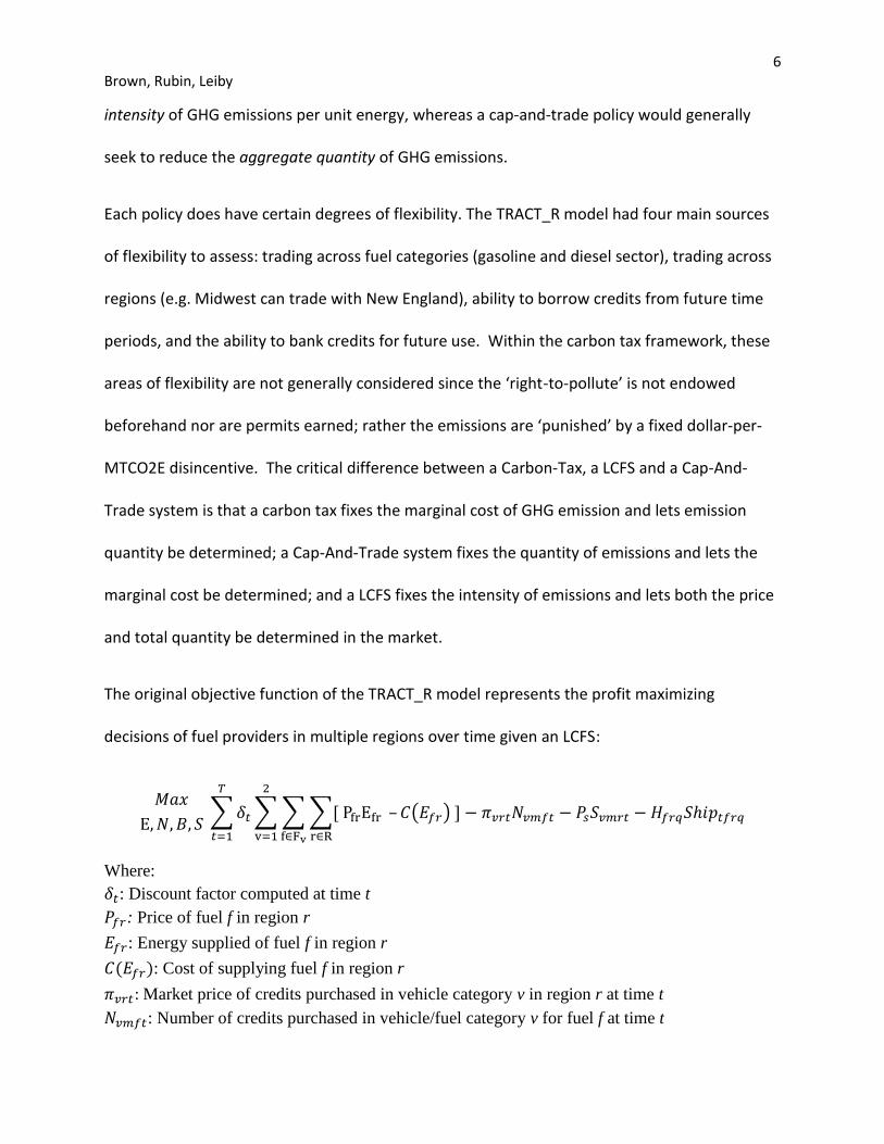
The original objective function of the TRACT_R model represents the profit maximizing

decisions of fuel providers in multiple regions over time given an LCFS:

∑ ∑ ∑ ∑

( )

Where:

: Discount factor computed at time t

: Price of fuel f in region r

: Energy supplied of fuel f in region r

: Cost of supplying fuel f in region r

: Market price of credits purchased in vehicle category v in region r at time t

: Number of credits purchased in vehicle/fuel category v for fuel f at time t

7 Brown, Rubin, Leiby

: Price of ‘safety valve’ credit s

: Number of safety valve credits purchased in vehicle category v in region r at time t

: Cost to ship fuel f from region r to region q

: Amount of fuel f shipped at time t from region r to region q

The maximization of these individual fuel provider objectives are subject to constraints on the

average CI and on credit banking/borrowing balances. Credit prices are endogenously

determined by the aggregate market-wide constraints on carbon intensity. Fuel prices P are also

endogenous given fuel supply-demand balance constraints.

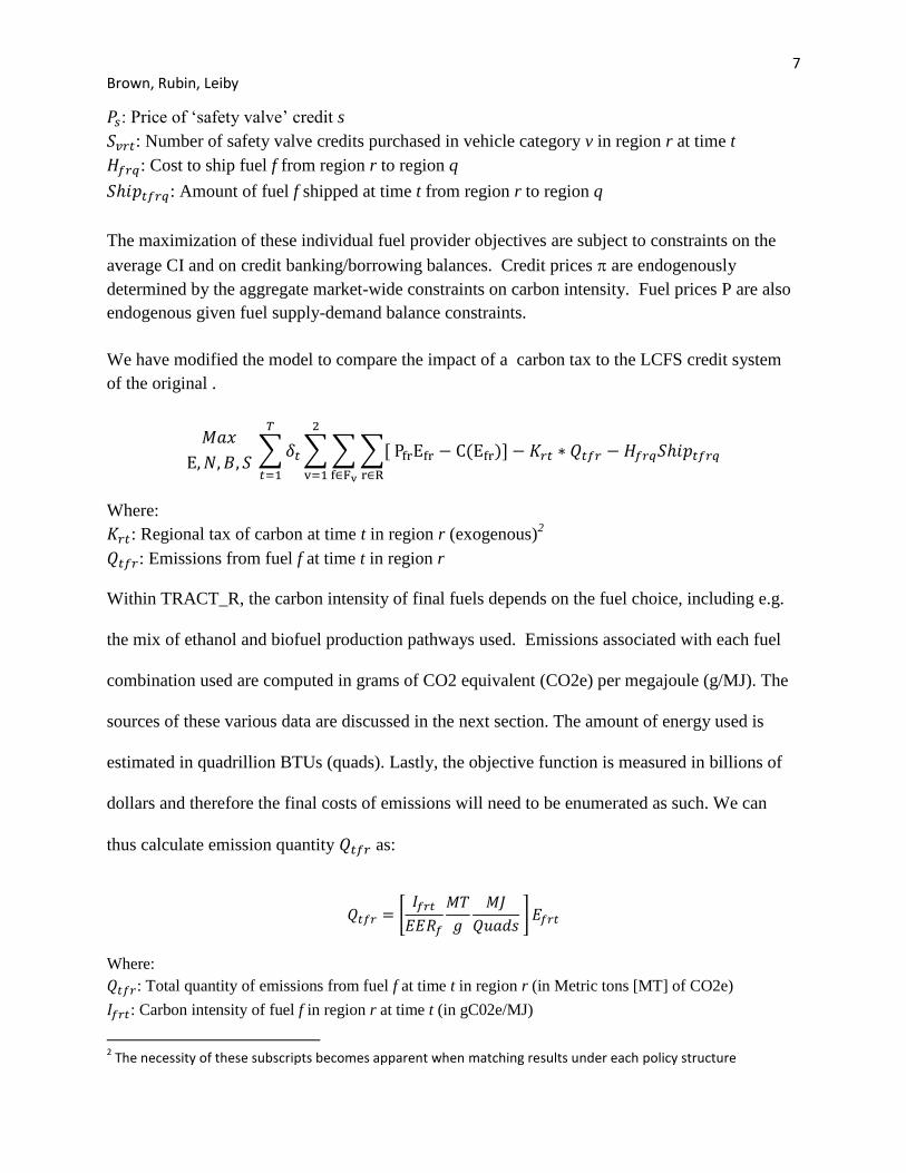
We have modified the model to compare the impact of a carbon tax to the LCFS credit system

of the original .

∑ ∑ ∑ ∑

Where:

: Regional tax of carbon at time t in region r (exogenous)2

: Emissions from fuel f at time t in region r

Within TRACT_R, the carbon intensity of final fuels depends on the fuel choice, including e.g.

the mix of ethanol and biofuel production pathways used. Emissions associated with each fuel

combination used are computed in grams of CO2 equivalent (CO2e) per megajoule (g/MJ). The

sources of these various data are discussed in the next section. The amount of energy used is

estimated in quadrillion BTUs (quads). Lastly, the objective function is measured in billions of

dollars and therefore the final costs of emissions will need to be enumerated as such. We can

thus calculate emission quantity as:

[

]

Where:

: Total quantity of emissions from fuel f at time t in region r (in Metric tons [MT] of CO2e)

: Carbon intensity of fuel f in region r at time t (in gC02e/MJ)

2 The necessity of these subscripts becomes apparent when matching results under each policy structure

8 Brown, Rubin, Leiby

: Energy efficiency ratio of fuel f, an adjustment factor for greater motive efficiency of some fuels,

e.g. electricity

: Metric tons per gram = 0.000001

: Megajoules per quadrillion BTU

: Energy used of fuel f in region r at time t in Quads

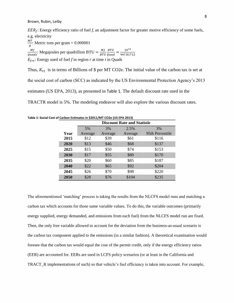
Thus, is in terms of Billions of $ per MT CO2e. The initial value of the carbon tax is set at

the social cost of carbon (SCC) as indicated by the US Environmental Protection Agency’s 2013

estimates (US EPA, 2013), as presented in Table 1. The default discount rate used in the

TRACTR model is 5%. The modeling endeavor will also explore the various discount rates.

Table 1: Social Cost of Carbon Estimates in $2011/MT CO2e (US EPA 2013)

Year

Discount Rate and Statistic

5%

Average

3%

Average

2.5%

Average

3%

95th Percentile

2015 $12 $39 $61 $116

2020 $13 $46 $68 $137

2025 $15 $50 $74 $153

2030 $17 $55 $80 $170

2035 $20 $60 $85 $187

2040 $22 $65 $92 $204

2045 $26 $70 $98 $220

2050 $28 $76 $104 $235

The aforementioned ‘matching’ process is taking the results from the NLCFS model runs and matching a

carbon tax which accounts for those same variable values. To do this, the variable outcomes (primarily

energy supplied, energy demanded, and emissions from each fuel) from the NLCFS model run are fixed.

Then, the only free variable allowed to account for the deviation from the business-as-usual scenario is

the carbon tax component applied to the emissions (in a similar fashion). A theoretical examination would

foresee that the carbon tax would equal the cost of the permit credit, only if the energy efficiency ratios

(EER) are accounted for. EERs are used in LCFS policy scenarios (or at least in the California and

TRACT_R implementations of such) so that vehicle’s fuel efficiency is taken into account. For example,

9 Brown, Rubin, Leiby

a megajoule of stored energy in an electric vehicle would allow further travel than in a conventional

internal combustion engine.

Data

The main sources of data for the TRACT_R model are the 2013 Annual Energy Outlook (US

EIA, 2013), the VISION model (Argonne National Laboratory, 2013), the Greenhouse Gases,

Regulated Emissions, and Energy Use in Transportation model (GREET; Argonne National

Laboratory, 2013), and the BioTrans model (Uria-Martinez et al, 2013). The Annual Energy

Outlook provides aggregate, regional energy estimations. The other models are used to delineate

energy usage by final category. The VISION model from ANL is a vehicle stock and energy

usage model from which the estimates and assumptions for electric vehicles are gathered.

BioTrans is used to construct regional supply curves for cellulosic ethanol production. To gather

region-specific biodiesel usage, national consumption is weighted by regional capacity.

The main source of carbon intensity (CI) data is GREET. Regional cellulosic ethanol CI is

computed using GREET cellulosic ethanol CIs weighted by the regional feedstock sources as

estimated in the BioTrans model. Regional electricity CI is computed using average of electricity

CI by source from GREET weighted by electricity generation by source from AEO 2012.

Petroleum fuel CIs by PADD are used to compute census division gasoline and diesel CIs by

weighting with 2011 state-level energy usage (US EIA, 2013). Corn ethanol, imported sugarcane

ethanol, biodiesel, FT-diesel, CNG and hydrogen CIs are set at national estimates from GREET

(ANL, 2012). PHEV CI is computed as the product of regional electricity and E10 CIs and

respective energy proportions from VISION 2012.

10 Brown, Rubin, Leiby

Results A primary result from this modeling is the final level of carbon emissions. Figure 1 presents the

values from a business-as-usual (BAU) scenario as well as scenarios with higher carbon tax

levels. A main conclusion from these scenarios is that there are declining returns in terms of

carbon abatement from increasing tax values. This is represented in the decreased gap between

the $40/MT and $50/MT scenarios; relative to all other scenario differences, the smallest gap in

aggregate emission reductions occurs between these scenarios.

Figure 1: National Emissions from Various Carbon Tax Levels

The declining returns of carbon reduction to an increasing carbon tax level are evident from the

changing decrements in U.S aggregate GHG emissions across tax levels in Figure 2. These

results are summarized in Table 2, which reports the cumulative reductions over the 24 year scenario

period. The rows of Table 2 can be summed to account for differences among scenarios (e.g. from

BAU to $20 / MT would be 1313 + 1217 = 2530 Million MT CO2e). The most apparent

difference in the carbon reductions across scenarios is when the carbon tax is increased from $40

11 Brown, Rubin, Leiby

/ MT to $50 / MT and the reduction in carbon is 216.8 million MT CO2e. This is consistent with

standard economic theory which suggests that the marginal cost of emission reductions should

increase with the stringency of the policy. That is, there no threshold effects or non-convexities

in the abatement marginal cost function (supply curve) implied by this model.

Table 2: Aggregated Emissions Reduction for Various Carbon Tax Levels

Scenarios compared Additional Amount of Emissions Reduction

(Million MT CO2e)

From BAU to $10 / MT 1313.3

From $10 / MT to $20 / MT 1217.8

From $20 / MT to $30 / MT 1128.6

From $30 / MT to $40 / MT 918.1

From $40 / MT to $50 / MT 216.8

Another concern is the demand response that a carbon tax would have on the final fuels. Given

the higher prices of fuels, consumers will respond with a reduction in final fuel consumption.

This is in contrast to the LCFS in that the LCFS will incentivize the consumption of lower-

carbon fuels (those with a carbon-intensity below the standard) instead of disincentivizing all

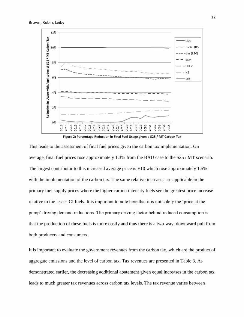
fuels consumed in proportion to their carbon intensity. Observing Figure 2, it becomes apparent

that the reduction of consumption in the higher carbon intensive fuels (CNG, gasoline, and

diesel) remains the most pertinent impact of the carbon tax. Overall, the $25 / MT carbon tax

amounts to a 6.4% reduction in national fuel usage relative to the BAU scenario over the 2012-

2035 time period.

12 Brown, Rubin, Leiby

Figure 2: Percentage Reduction in Final Fuel Usage given a $25 / MT Carbon Tax

This leads to the assessment of final fuel prices given the carbon tax implementation. On

average, final fuel prices rose approximately 1.3% from the BAU case to the $25 / MT scenario.

The largest contributor to this increased average price is E10 which rose approximately 1.5%

with the implementation of the carbon tax. The same relative increases are applicable in the

primary fuel supply prices where the higher carbon intensity fuels see the greatest price increase

relative to the lesser-CI fuels. It is important to note here that it is not solely the ‘price at the

pump’ driving demand reductions. The primary driving factor behind reduced consumption is

that the production of these fuels is more costly and thus there is a two-way, downward pull from

both producers and consumers.

It is important to evaluate the government revenues from the carbon tax, which are the product of

aggregate emissions and the level of carbon tax. Tax revenues are presented in Table 3. As

demonstrated earlier, the decreasing additional abatement given equal increases in the carbon tax

leads to much greater tax revenues across carbon tax levels. The tax revenue varies between

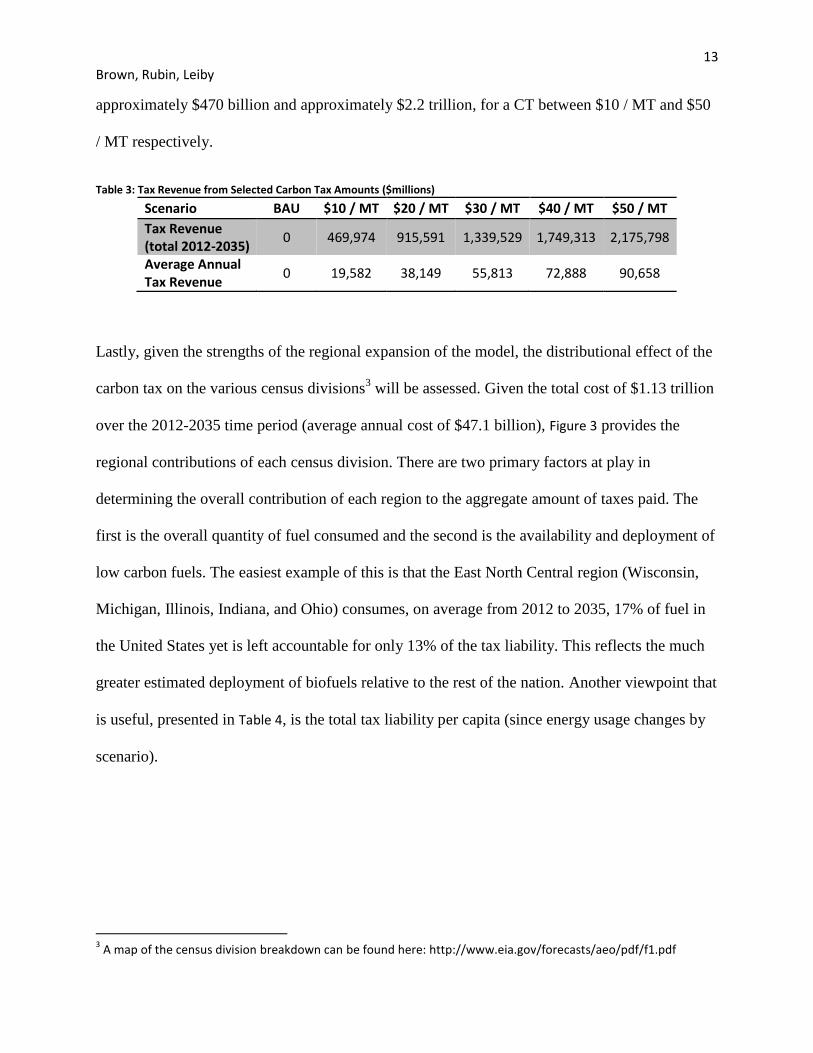
13 Brown, Rubin, Leiby

approximately $470 billion and approximately $2.2 trillion, for a CT between $10 / MT and $50

/ MT respectively.

Table 3: Tax Revenue from Selected Carbon Tax Amounts ($millions)

Scenario BAU $10 / MT $20 / MT $30 / MT $40 / MT $50 / MT

Tax Revenue (total 2012-2035)

0 469,974 915,591 1,339,529 1,749,313 2,175,798

Average Annual Tax Revenue

0 19,582 38,149 55,813 72,888 90,658

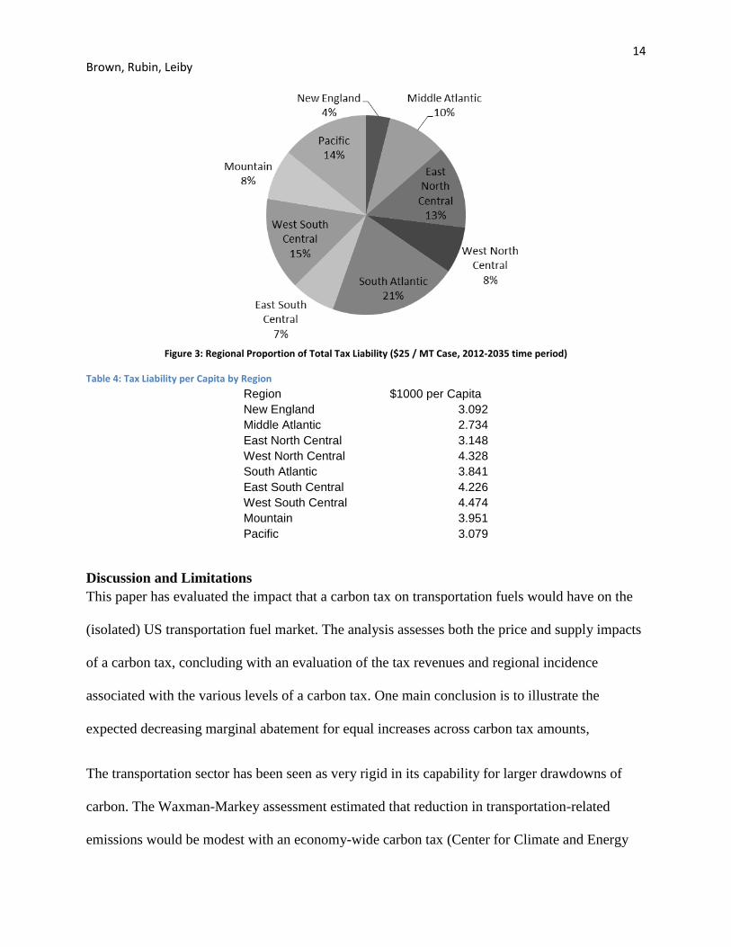
Lastly, given the strengths of the regional expansion of the model, the distributional effect of the

carbon tax on the various census divisions3 will be assessed. Given the total cost of $1.13 trillion

over the 2012-2035 time period (average annual cost of $47.1 billion), Figure 3 provides the

regional contributions of each census division. There are two primary factors at play in

determining the overall contribution of each region to the aggregate amount of taxes paid. The

first is the overall quantity of fuel consumed and the second is the availability and deployment of

low carbon fuels. The easiest example of this is that the East North Central region (Wisconsin,

Michigan, Illinois, Indiana, and Ohio) consumes, on average from 2012 to 2035, 17% of fuel in

the United States yet is left accountable for only 13% of the tax liability. This reflects the much

greater estimated deployment of biofuels relative to the rest of the nation. Another viewpoint that

is useful, presented in Table 4, is the total tax liability per capita (since energy usage changes by

scenario).

3 A map of the census division breakdown can be found here: http://www.eia.gov/forecasts/aeo/pdf/f1.pdf

14 Brown, Rubin, Leiby

Figure 3: Regional Proportion of Total Tax Liability ($25 / MT Case, 2012-2035 time period)

Table 4: Tax Liability per Capita by Region

Region $1000 per Capita

New England 3.092

Middle Atlantic 2.734

East North Central 3.148

West North Central 4.328

South Atlantic 3.841

East South Central 4.226

West South Central 4.474

Mountain 3.951

Pacific 3.079

Discussion and Limitations

This paper has evaluated the impact that a carbon tax on transportation fuels would have on the

(isolated) US transportation fuel market. The analysis assesses both the price and supply impacts

of a carbon tax, concluding with an evaluation of the tax revenues and regional incidence

associated with the various levels of a carbon tax. One main conclusion is to illustrate the

expected decreasing marginal abatement for equal increases across carbon tax amounts,

The transportation sector has been seen as very rigid in its capability for larger drawdowns of

carbon. The Waxman-Markey assessment estimated that reduction in transportation-related

emissions would be modest with an economy-wide carbon tax (Center for Climate and Energy

15 Brown, Rubin, Leiby

Solutions, 2010). The reductions would contribute between only 1% to 3.5% of total reductions

by 2020 and 2.6% to 8.5% of total reductions by 2030. Our results indicate a carbon tax of

$50/MT is needed for about a 10% reduction in vehicle GHG emissions. In this analysis, the

carbon tax was more effective than an LCFS, but reduced emissions primarily through the

reduction of total fuels consumed and not from substituting in lower-CI fuels such as an LCFS

(Rubin et al. 2014).

One primary feature of this investigation is that the transportation fuel market is the only market

affected by the carbon tax. In this sense, the analysis isolates the impacts that the carbon tax

would have on the economy and limits the investigation to only the transportation fuel market.

The results should be taken in this sense and the reader should be aware that a more complete

cost-effectiveness assessment would include other sources of emissions as well (e.g. power

companies and distributors). The estimated impact is therefore limited to the light and heavy

duty vehicle sectors in the United States.

Another limitation is that the rates of carbon of emission per unit of primary fuel are considered

fixed. An extension could be to include the capabilities for fuel producers to reduce the carbon

intensity of their fuel blends through various means. One method is through carbon capture and

sequestration in the production of fossil fuels. Another conflicting source of carbon intensity

inaccuracies is in the potentially greater (or lesser) usage of higher-carbon intensity oil from the

Canadian Oil Sands. A further extension of this modeling effort would be to evaluate the how

changing domestic and international market for crude oil supply and trade could alter the

estimated CI of petroleum fuels.

16 Brown, Rubin, Leiby

References

ANL Transportation Technology R&D Center. GREET model: The greenhouse gases, regulated

emissions, and energy use in transportation model. 2012.

ANL Transportation Technology R&D Center. The VISION model. 2012.

Center for Climate Energy Solutions 2010. Economic Insight from Modeling Anlyses of HR

2454. Retrieved April 7, 2014 from: http://www.c2es.org/docUploads/economic-insights-

hr2454.pdf

Chen, X and M Khanna. The Market-Mediates Effects of Low Carbon Fuel Policies. The Journal

of Agrobiotechnology Management and Economics. Volume 15, Number 1, Article 11.

Available at: http://www.agbioforum.org/v15n1/v15n1a11-khanna.htm

Executive Office of the President (2013). The President's Climate Action Plan.

Hartgen et al 2011. Impacts of Transportation Policies on Greenhosue Gas Emissions in US

Regions. Reason Policy Study 387, published November 2011.

Huang, H., M. Khanna, et al. (2013). "Stacking low carbon policies on the renewable fuels

standard: Economic and greenhouse gas implications." Energy Policy 56(0): 5-15.

Parry, I and R Williams 2010. Is a Carbon Tax the Only Good Climate Policy? Options to Cut

CO2 Emissions. Resources Magazine, retrieved 02/19/2014 from:

http://www.rff.org/Publications/Resources/Pages/Is-a-Carbon-Tax-the-Only-Good-Climate-

Policy-176.aspx

Rubin, J., P Leiby, and M Brown 2014. Regional Credit Trading: Economic and GHG Impacts of

a National Low Carbon Fuel Standard. In Press, Transportation Research Record.

Tate, E., O. Harpster, et al. (2008). The Electrification of the Automobile: From Conventional

Hybrid, to Plug-in Hybrids, to Extended-Range Electric Vehicles. Retrieved 02/19/2014 from

http://www.media.gm.com/content/dam/Media/microsites/product/volt/docs/paper.pdf.[doi:10.42

71/2008-01-0458]

Uría-Martínez R, Leiby P. Advanced biofuels system configuration in the U.S.: Cost and

performance tradeoffs. Seattle, Washington. Agricultural & Applied Economics Association;

2012.

US EIA 2013. Annual Energy Outlook 2013. Retrieved 02/19/2014 from:

http://www.eia.gov/forecasts/aeo/er/index.cfm

US EPA 2010. Sources of Greenhouse Gas Emissions. Retrieved 02/19/2014 from:

http://www.epa.gov/climatechange/ghgemissions/sources/transportation.html

US EPA 2013. Technical Update of the Social Cost of Carbon for Regulatory Impact Analysis. May 2013. Retrieved April 4th, 2014 from: http://www.whitehouse.gov/sites/default/files/omb/assets/inforeg/technical-update-social-cost-of-carbon-for-regulator-impact-analysis.pdf

US NHTSA 2012. Research Supporting 2017-2025 CAFE Final Rule. Retrieved 02/19/2014

from: http://www.nhtsa.gov/Laws+&+Regulations/CAFE+-

+Fuel+Economy/Research+Supporting+2017-2025+CAFE+Final+Rule

17 Brown, Rubin, Leiby

Yeh, S. and D. Sperling (2010). "Low carbon fuel standards: Implementation scenarios and

challenges." Energy Policy 38(11): 6955-6965.

Yeh, S., D. Sperling, et al. (2012). "National Low Carbon Fuel Standard: Technical Analysis

Report." Social Science Research Network.