RS2005.tex

Eurosystem Monetary Targeting:Lessons from U.S. Data¤

Glenn D. Rudebuschy Lars E.O. Svenssonz

First draft: May 1999This version: May 2000

Abstract

Using a small empirical model of in‡ation, output, and money estimated on U.S. data,we compare the relative performance of monetary targeting and in‡ation targeting. The re-sults show that monetary targeting would be quite ine¢cient, with both higher in‡ation andoutput variability. This is true even with a nonstochastic money demand formulation. Ourresults are also robust to using a P* model of in‡ation. Therefore, in these popular frame-works, there is no support for the prominent role given to money growth in the Eurosystem’smonetary policy strategy.

JEL Classi…cation: E42, E52, E58

Keywords: in‡ation targeting, monetary targeting, ECB

¤We thank Jordi Gali, Henrik Jensen, Edward Nelson, Athansios Orphanides, David Small, Ulf Söderströmand the editors and two anonymous referees for comments, Niloofar Badie for research assistance, and ChristinaLönnblad for editorial and secretarial assistance. The views expressed in the paper do not necessarily re‡ect theviews of the Federal Reserve Bank of San Francisco or the Federal Reserve System.

yFederal Reserve Bank of San Francisco; Glenn.Rudebusch@sf.frb.org, http://www.frbsf.org/econrsrch/economists/grudebusch.html.

zInstitute for International Economic Studies, Stockholm University; CEPR and NBER; Lars.Svensson@iies.su.se, http://www.iies.su.se/leosven/.

1. Introduction

The recent formation of a new monetary institution in Europe has, once more, highlighted the

question of the proper role for money in the conduct of monetary policy. In the past few years,

particularly during the gestation of the European Central Bank (ECB), a lively debate has

considered whether monetary targeting or in‡ation targeting would be the most appropriate

monetary strategy for the Eurosystem.1 This debate was only spurred on by the Eurosystem’s

announcement of its actual monetary strategy. As described in the inaugural issue of the ECB’s

Monthly Bulletin [10, p. 9]:

. . . [T]he strategy is based on two pillars. The …rst consists in a prominent rolefor money, as signalled by the announcement of a quantitative reference value of4-1/2 percent for the growth rate of the broad monetary aggregate M3 which isregarded as being compatible with price stability. The second comprises a broadlybased assessment of the outlook for price developments and the risks to price stabilityusing …nancial and other economic indicators.

This strategy appears to be a combination of a weak type of monetary targeting and an

implicit form of in‡ation targeting. It is only a weak type of monetary targeting because the

Eurosystem has rejected a simple formulation in which money growth is an intermediate target

variable to always be brought in line with the reference value. Nevertheless, the Eurosystem

has made it clear that deviations of money growth from the reference value will be treated as

a major factor in its policy decisions. The second pillar contains the basic thrust of in‡ation

targeting; however, some of the important elements of an explicit in‡ation targeting strategy,

such as the public comparison of an in‡ation forecast to an announced target, are absent.

In order to understand the potential for success of this mixed strategy for monetary policy,

this paper evaluates the relative performance of monetary targeting and in‡ation targeting.

This exercise provides, in a loose sense, some evidence of the relative value of the …rst and

second pillars of Eurosystem strategy. Previous analysis in Svensson [41], [42], and [44] provides

a theoretical case for favoring in‡ation targeting over monetary targeting. In this paper, we

provide an empirical counterpart to this analysis using a small estimated model of in‡ation,

output, and money.

Of course, an important di¢culty for our analysis, or indeed any empirical investigation of

the policy choice faced by the Eurosystem, is the lack of a data set with which to estimate an

1 The Eurosystem, which consists of the ECB and the national central banks of the 11 countries that haveadopted the euro, has conducted monetary policy for the euro area since January 1, 1999.

1

empirical model of the euro-area economy. The 11 nations of the euro area have been bound

together with a common currency for only a very short period, so using appropriate post-

union euro-area data for model estimates is not an option. Constructing synthetic pre-union

aggregates from the separate historical data for the 11 euro-area countries is one alternative.2

This, of course, is an ambiguous counter-factual exercise. National statistics with di¤ering

de…nitions must be aggregated, and some accounting must be made of the actual historical

exchange rate ‡uctuations among the 11 euro-area countries. Furthermore, even if unambiguous

pre-union aggregates were available, it is not clear that the experience of the euro area before

monetary union under ‡oating exchange rates and with a variety of monetary policy regimes and

institutions would be appropriate for analyzing the post-union euro area under the Eurosystem.

Thus, reconstructed historical euro-area data will be an uncertain guide to the future. The

experience of the United States is, in our opinion, at least as relevant a guide. It is often

noted that the euro area has many similarities to the United States—obviously in terms of a

monetary union—but also in economic size and in the relative importance of external trade.

Accordingly, in analyzing the relative value of monetary targeting and in‡ation targeting, we

use coe¢cients in our model that are estimated using U.S. data. We certainly cannot guarantee

that this empirical model, which is merely a rudimentary approximation of the U.S. economy, is

the correct vehicle for analyzing euro-area monetary policy in the future; however, as outlined in

the next section, we think that our model has some desirable attributes even from a European

perspective. Still, a major caveat to our analysis is that the economy in the euro-area under the

Eurosystem may behave substantially di¤erent from the U.S. experience (or from a reconstructed

euro-area history).3

With that caveat clearly established, our results from a model …t to the U.S. economy are

used to draw some lessons for the Eurosystem. Our results show that monetary targeting is

much more ine¢cient, in the sense of inducing more variable in‡ation and output, than in‡ation

targeting. We get this result even after excluding parts of the sample period so as to estimate a

very well-behaved, nonstochastic money-demand equation. Furthermore, this result is true even

if we assume that there are no stochastic shocks at all a¤ecting money demand. Thus, counter

to conventional wisdom, monetary targeting is ine¢cient even if money demand is stable and

controllable. This result re‡ects the fact that given the dynamics of how money is related to the

2 This route is followed by Peersman and Smets [33] and Taylor [49], who use data from a subset of the 11euro-area countries, and Gerlach and Svensson [14], who use data for the whole euro area.

3 Indeed, for what it is worth, as noted in section 2, the work of Peersman and Smets [33] and Taylor [49]suggests that the equations of our model also have some claim to …t the pre-union synthetic euro-area data.

2

rest of the economy, money growth is a poor predictor of future in‡ation (in the sense that the

correlation between money growth and in‡ation forecasts is quite low). Thus, money growth

is an inadequate indicator of risks to price stability. All this provides substantial empirical

con…rmation of the theoretical arguments in Svensson [41], [42], and [44].

Section 2 presents the model and the empirical estimates. Section 3 reports the results on the

relative performance of in‡ation targeting and monetary targeting. We also show that nominal

GDP targeting—a close relative to monetary targeting—would be quite ine¢cient compared

to in‡ation targeting. In section 3, we also consider an alternative model that incorporates

a P* equation for in‡ation, which has had some empirical success in both the U.S. (Hallman,

Porter, and Small [17]) and in the euro area (Gerlach and Svensson [14]). However, even with the

enhanced role for money in the P* model, we …nd no support for money-growth targeting, which

provides empirical con…rmation of the theoretical results of Svensson [46]. Section 4 discusses

the lessons for the Eurosystem. Section 5 presents some conclusions.

2. An Empirical Model of U.S. Output, In‡ation, and Money

2.1. Aggregate supply and demand

The two equations for output and in‡ation used for our baseline analysis, which are fully de-

scribed in Rudebusch and Svensson [36], are

¼t+1 = ®¼1¼t + ®¼2¼t¡1 + ®¼3¼t¡2 + ®¼4¼t¡3 + ®yyt + "t+1 (2.1)

yt+1 = ¯y1yt + ¯y2yt¡1 ¡ ¯r (¹{t ¡ ¹¼t ¡ ¹r) + ´t+1; (2.2)

where ¼t is quarterly in‡ation in the GDP chain-weighted price index (Pt) in percent at an

annual rate, i.e., ¼t ´ 4(pt ¡ pt¡1), where pt = 100 lnPt, ¹¼t is four-quarter in‡ation in the

GDP chain-weighted price index, i.e., 14§3j=0¼t¡j , it is the quarterly average federal funds rate

in percent per year, ¹{t is the four-quarter average federal funds rate, i.e., 14§3j=0it¡j, and yt is the

output gap, the relative gap between actual real GDP (Qt) and potential GDP (Q¤t ) in percent,

i.e., 100(Qt ¡Q¤t )=Q¤t (approximately qt ¡ q¤t , where qt ´ 100 lnQt and q¤t ´ 100 lnQ¤t are logGDP and log potential GDP scaled by 100, respectively). The series on potential GDP (Q¤t ) is

obtained from the Congressional Budget O¢ce [7]. The constant ¹r is the average real interest

rate, and "t and ´t are iid shocks with variances ¾2" and ¾

2´. The …ve variables were de-meaned

prior to estimation, so no constants appear in the equations and ¹r is set equal to zero.

3

Estimated versions of these equations, using the sample period 1961:1 to 1996:4, are (with

coe¢cient standard errors given in parentheses)

¼t+1 = :675 ¼t ¡ :077 ¼t¡1 + :286 ¼t¡2 + :115 ¼t¡3 + :152 yt + "t+1;(:083) (:103) (:107) (:088) (:037)

(2.3)

R̄2 = :81; SE = 1:084; DW = 1:99;

yt+1 = 1:161 yt ¡ :259 yt¡1 ¡ :088 (¹{t ¡ ¹¼t) + ´t+1;(:079) (:077) (:032)

(2.4)

R̄2 = :90; SE = 0:823; DW = 2:08:

The equations were estimated individually by OLS.4 The hypothesis that the sum of the

lag coe¢cients of in‡ation equals one had a p-value of .48, so this restriction was imposed in

estimation. Thus, this is an accelerationist form of the Phillips curve, which implies a long-run

vertical Phillips curve.5

The use of this model can be motivated by a variety of considerations. In particular, although

its simple structure facilitates the production of benchmark results, as described by Rudebusch

and Svensson [36], this model also appears to roughly capture the views about the dynamics of

the economy held by many monetary policymakers. The empirical …t of the model is also quite

good compared, for example, to an unrestricted VAR. Indeed, the model can be interpreted as

a restricted VAR, where the restrictions imposed are not at odds with the data as judged, for

example, with standard model information criteria (see Rudebusch and Svensson [36]).6

Finally, the model appears to be stable over various subsamples—an important condition

for drawing inference. With a backward-looking model, the Lucas Critique may apply with

particular force, so it is important to gauge its historical importance with econometric stability

tests (Oliner, Rudebusch, and Sichel [29]). For example, consider a stability test from Andrews

[1]: the maximum value of the likelihood-ratio test statistic for structural stability over all

possible breakpoints in the middle 70 percent of the sample. For our estimated in‡ation equation,

the maximum likelihood-ratio test statistic is 10.89 (in 1972:3), while the 10 percent critical value

is 14.31 (from Table 1 in Andrews [1]). Similarly, for the output equation, the maximum statistic

is 11.51 (in 1982:4), while the 10 percent critical value is 12.27.4 The estimates are slightly di¤erent from those in Rudebusch and Svensson [36] because of data revisions and

a longer sample.5 Using reconstructed historical euro-area data, this model has been estimated by Peersman and Smets [33]

and Taylor [49]. They have obtained coe¢cient estimates that are close to our U.S. ones, although with lowerin‡ation persistence.

6 Söderström [39] scrutinizes the Rudebusch-Svensson model further.

4

2.2. Adding money to the model

Money could be added to the aggregate supply and demand model described above in a variety

of ways. Just as for our selection of equations (2.1) and (2.2), three considerations motivate

our choice of a model with money: simplicity, congruence with actual central bank models,

and empirical …t to the data. Perhaps most importantly, we add money to the model not

as a “straw man”, but in a fashion consistent with the views of monetary policymakers.7 As a

general characterization, central bankers typically hold the view that movements in the monetary

aggregates play essentially no role in the direct quarter-by-quarter determination of either output

or prices; however, a sizable fraction also concedes that money may have some value as an

indicator of economic developments (e.g., Meyer [26]).

This view of the role of monetary aggregates is evident in most central bank empirical policy

models. For example, Smets [37] surveys the central bank models from 12 di¤erent countries

(including 6 of the countries in the euro area) and notes:

In most of the central banks’ macroeconometric models the transmission mechanismof monetary policy is modelled as an interest rate transmission process. The cen-tral bank sets the short-term interest rate, which in‡uences interest rates over thewhole maturity spectrum, other asset prices, and the exchange rate. These changesin …nancial variables then a¤ect output and prices through the di¤erent spendingcomponents. The role of money is in most cases a passive one, in the sense thatmoney is demand determined. [37, p. 226]

Our model will incorporate money in an identical fashion. The alternative, where money

plays a direct role in output or in‡ation determination separate from interest rates, has little

support among central banks or in the data.8 For example, Gerlach and Smets [13] …t small

(output, in‡ation, and interest rate) VARs to each of the G7 countries and state: “In preliminary

work we incorporated monetary aggregates (M3 or M2) in the analysis, but found that they

appear largely determined by money demand shocks that in turn have little, if any, impact on

the economy” (p. 191). Similarly, in our AD-AS structural model, lags of money (in levels or

growth rates) were invariably insigni…cant when added to equations (2.1) and (2.2).

7 Our analysis of money will be most convincing to central bankers (including those in the Eurosystem, whoare, of course, among the most important ultimate consumers of this research) if using a model that is similar tothe ones actually employed.

8 There are two primary channels for the quantity of money to a¤ect aggregate demand directly: a realbalance e¤ect and a bank lending channel. The lack of U.S. evidence for either of these two channels is noted in,respectively, Reifschneider, et al. [32] and Oliner and Rudebusch [28]. Meltzer [24] and Nelson [27] …nd evidenceof an e¤ect of real money on aggregate demand; the latter interprets this as a proxy for an e¤ect via a long interestrate. The weak contribution of money in predicting in‡ation is described in Estrella and Mishkin [11] and Stockand Watson [40].

5

Probably the most important exception to this general lack of interest in incorporating money

directly into an AD-AS model is the P ¤ model of Hallman, Porter, and Small [17]. This model,

which is still only rarely used, has been estimated with reconstructed euro-area data in Gerlach

and Svensson [14]. Results with an alternative P ¤ in‡ation equation will be examined separately

in subsection 3.3 below.

Instead, following the mainstream, we add money to our model with a separate money-

demand equation, which is cast in a standard error-correction form. The long-run money-demand

function is

mt = qt ¡ ·iit; (2.5)

where mt is the log of real M2 (scaled by 100), i.e., 100 ln M2tPt. In the long run, the demand for

real money moves one-for-one with real output9 and negatively with respect to the interest rate

(a proxy for the opportunity cost of money10), so ·i, the long-run interest rate semielasticity, is

positive. The short-run money-demand equation takes the form

¢mt+1 = ¡·m(mt ¡ qt + ·iit) + ·1¢mt + »t+1, (2.6)

where ¢mt+1 ´ mt+1 ¡mt is the growth rate of real money measured in percent per quarter,and »t is an iid shock with variance ¾

2» . Assuming that the stock of real money adjusts to its

long run average, qt ¡ ·iit, the error-correction coe¢cient ·m should be positive.Before providing estimates of the money demand equation, it is instructive to examine the

long-run equilibrium condition (2.5). Figure 2.1 shows the log of M2 velocity (that is, vt ´qt¡mt) and the interest rate (it). According to condition (2.5), these two variables should movetogether so that their di¤erence is stationary. For most of the sample, this clearly appears to

be the case (and, for example, Hallman, Porter and Small [17] provide supporting statistical

evidence). In the 1990’s, however, there was a dramatic increase in velocity, and the historical

long-run relationship obviously broke down. The cause of this upward shift in velocity is still

debated, but it is likely linked to the increased availability and liquidity of bond and stock9 When tested, we could not reject a unitary income elasticity (the p-value is .16), so it is imposed. This is

consistent with previous empirical investigations such as Feldstein and Stock [12] and Porter and Small [31].10 Models of money with more institutional detail calculate the opportunity cost as the di¤erence between the

alternative rate for assets that are substitutes to money and the own-rate on money deposits. In the U.S., thealternative rate is typically a short-term rate like a 3-month Treasury bill rate, and the own-rate is the averagerate on deposits in money market deposit accounts, small time deposit accounts, and so forth (e.g., Porter andSmall [31]). However, since deposit rates are quite sluggish, much of the variation in such an opportunity costcan be captured with just the alternative rate, which, in our case, is proxied by the funds rate. (See, for example,…gure 3 in Porter and Small [31].) In contrast, some studies employ the short rate as the own rate and a long-termmarket interest rate as the alternative rate (e.g., Hamburger [18]). However, simply enlarging our structural modelto include a rational expectations model of the long-term yield is likely insu¢cient (see Hess, Jones, and Porter[19]), and modeling the relevant term premia are well beyond the scope of our investigation.

6

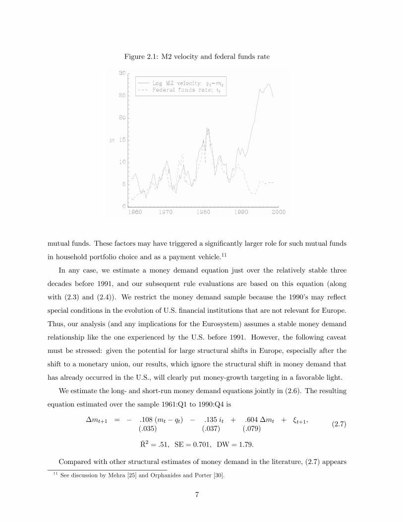
Figure 2.1: M2 velocity and federal funds rate

mutual funds. These factors may have triggered a signi…cantly larger role for such mutual funds

in household portfolio choice and as a payment vehicle.11

In any case, we estimate a money demand equation just over the relatively stable three

decades before 1991, and our subsequent rule evaluations are based on this equation (along

with (2.3) and (2.4)). We restrict the money demand sample because the 1990’s may re‡ect

special conditions in the evolution of U.S. …nancial institutions that are not relevant for Europe.

Thus, our analysis (and any implications for the Eurosystem) assumes a stable money demand

relationship like the one experienced by the U.S. before 1991. However, the following caveat

must be stressed: given the potential for large structural shifts in Europe, especially after the

shift to a monetary union, our results, which ignore the structural shift in money demand that

has already occurred in the U.S., will clearly put money-growth targeting in a favorable light.

We estimate the long- and short-run money demand equations jointly in (2.6). The resulting

equation estimated over the sample 1961:Q1 to 1990:Q4 is

¢mt+1 = ¡ :108 (mt ¡ qt) ¡ :135 it + :604 ¢mt + »t+1;(:035) (:037) (:079)

(2.7)

R̄2 = :51; SE = 0:701; DW = 1:79:

Compared with other structural estimates of money demand in the literature, (2.7) appears

11 See discussion by Mehra [25] and Orphanides and Porter [30].

7

to be a simple but reasonable representation.12 The value of the error correction coe¢cient (·m)

indicates that about 11 percent of the gap from the long-run equilibrium is closed each quarter.

This is essentially the same convergence rate estimated in Mehra [25] and in Porter and Small

[31] in much larger and more detailed money demand models. In addition, these authors provide

estimates of the dynamic responses and the interest rate semi-elasticity of money that are also

quite close to our own (·i = 1:25) (after accounting for our scaling of mt).

Finally, as noted above, structural stability is an important condition for policy inference.

Given the spectacular failures that have littered this …eld (e.g., the collapse of the Baba, Hendry,

and Starr [3] model described in Hess, Jones, and Porter [19]), we only humbly note that over our

shortened sample, the stability of our money demand equation is not rejected by the Andrews

test (described above). Speci…cally, the maximum value of the likelihood-ratio test statistic for

structural stability over all possible breakpoints is 9.91 (in 1981:1), while the 10 percent critical

value is 12.27 (from Table 1 in Andrews [1]).

2.3. The loss function and the optimal policy

Thus, equations (2.1), (2.2), and (2.6) provide the aggregate supply, aggregate demand, and

money-demand equations of the empirical model of the U.S. economy. To complete the model,

we specify the relationship among output, the output gap, and potential output,

yt ´ qt ¡ q¤t ; (2.8)

and make the assumption that potential output is a random walk,

q¤t+1 = q¤t + µt+1, (2.9)

where µt+1 is an iid shock with variance ¾2µ and mean ¹µ representing the upward growth of the

economy.

We furthermore specify a loss function that allows us to compare in‡ation targeting and

money-growth targeting in a convenient way. We assume that the relevant target variable under

money-growth targeting is the four-quarter money growth rate, ¹t, de…ned as

¹t ´ (mt + pt)¡ (mt¡4 + pt¡4) = mt ¡mt¡4 + ¹¼t (2.10)

12 Estimates of such error correction money demand equations using reconstructed historical euro-area aggre-gates are surveyed in Browne, Fagan and Henry [5]. The associated coe¢cients estimates appear to be broadlyin line to our U.S. estimates.

8

(recall that mt is (log) real money). For convenience we set the in‡ation target and the money-

growth targets to zero, so ¼t, ¹¼t and ¹t can be interpreted as deviations from the target. We

then assume the loss function

¸¼Var [¹¼t] + ¸yVar[yt] + ¸¹Var[¹t] + ¸¢iVar [it ¡ it¡1] ; (2.11)

where the parameters ¸¼; ¸y; ¸¹; ¸¢i ¸ 0 are the weights on in‡ation stabilization around the

in‡ation target, output-gap stabilization, money-growth stabilization around the money-growth

target, and interest-rate smoothing, respectively. We normalize the weights to sum to one.

Throughout, we assume the weight ¸¢i = 0:2, which corresponds to the standard weight on

interest-rate smoothing in Rudebusch and Svensson [36]. Given the weight on interest-rate

smoothing, we here de…ne ‡exible in‡ation targeting (FIT) as ¸¼ = ¸y = 0:4, ¸¹ = 0; strict

in‡ation targeting (SIT) as ¸¼ = 0:8, ¸y = ¸¹ = 0; strict output-gap targeting (SOT) as ¸y = 0:8,

¸¼ = ¸¹ = 0; and strict money-growth targeting (SMT) as ¸¹ = 0:8, ¸¼ = ¸y = 0.13 Flexible

in‡ation targeting corresponds to the standard case examined in Rudebusch and Svensson [36].14

Minimizing the loss function (2.11) for given weights and the model (2.1), (2.2) and (2.6)–

(2.10), results in an optimal reaction function

it = fXt; (2.12)

where f is a row vector and Xt is a vector of the state variables. Then the variances of the

goal variables are easily calculated.15 By varying the weights, we can calculate the reaction

function and the variances of the goal variables for each targeting case. We use the empirical

parameters of (2.1), (2.2) and (2.6), with ¾" = 1:08; ¾´ = 0:82 and ¾» = 0:70. The actual ¾µ

for our potential output series is equal to 0:19; however, this series is essentially a segmented

deterministic trend with infrequent breaks; thus, we set ¾µ equal to zero, which we interpret as

corresponding to a …xed trend.16

3. The e¢ciency frontier and monetary targeting for the U.S.

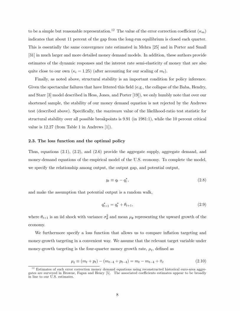
Figure 3.1 summarizes the results on the e¢ciency frontier for in‡ation and output-gap variances

for the di¤erent targeting cases (¼b in the …gure denotes ¹¼). The solid line shows the e¢ciency

13 Note that, as dicussed in Rudebusch and Svensson [36], we use the term “targeting” to refer to the mini-mization of a loss function over expected future deviations of the target variable from a desired level.14 Rudebusch and Svensson [36] use the weights ¸¼ = ¸y = 1 and ¸º = 0:5 in their standard case.15 An appendix available at the authors’ websites provides technical details.16 Smets [38] generalizes our model to allow for a stochastic trend in potential output, and he obtains an

estimate of ¾µ = 0:73: Our results were robust to variation in ¾µ.

9

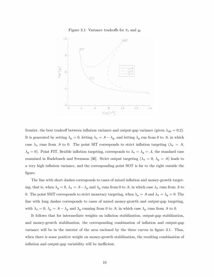
Figure 3.1: Variance tradeo¤s for ¹¼t and yt

frontier, the best tradeo¤ between in‡ation variance and output-gap variance (given ¸¢i = 0:2).

It is generated by setting ¸¹ = 0, letting ¸¼ = :8¡ ¸y, and letting ¸y run from 0 to :8, in which

case ¸¼ runs from .8 to 0. The point SIT corresponds to strict in‡ation targeting (¸¼ = :8,

¸y = 0). Point FIT, ‡exible in‡ation targeting, corresponds to ¸¼ = ¸y = :4, the standard case

examined in Rudebusch and Svensson [36]. Strict output targeting (¸¼ = 0, ¸y = :8) leads to

a very high in‡ation variance, and the corresponding point SOT is far to the right outside the

…gure.

The line with short dashes corresponds to cases of mixed in‡ation and money-growth target-

ing, that is, when ¸y = 0, ¸¼ = :8¡¸¹ and ¸¹ runs from 0 to .8, in which case ¸¼ runs from .8 to0. The point SMT corresponds to strict monetary targeting, when ¸¹ = :8 and ¸¼ = ¸y = 0: The

line with long dashes corresponds to cases of mixed money-growth and output-gap targeting,

with ¸¼ = 0, ¸¹ = :8¡ ¸y and ¸y running from 0 to .8, in which case ¸¹ runs from .8 to 0.

It follows that for intermediate weights on in‡ation stabilization, output-gap stabilization,

and money-growth stabilization, the corresponding combination of in‡ation and output-gap

variance will be in the interior of the area enclosed by the three curves in …gure 3.1. Thus,

when there is some positive weight on money-growth stabilization, the resulting combination of

in‡ation and output-gap variability will be ine¢cient.

10

Table 1. Variances and lossesCase ¸¼ ¸y ¸¹ ¸g Var ¹¼t Var yt Var¹t Var¢it Var¢4mt Var gt Loss1. FIT .4 .4 0 0 5.14 5.14 18.68 3.15 19.92 7.99 4.742. SIT .8 0 0 0 3.71 8.67 34.11 4.45 43.51 6.93 5.843. SOT 0 .8 0 0 46499 2.90 46506 1.61 8.92 46502 186014. SMT 0 0 .8 0 9.93 9.72 8.00 5.06 12.32 9.29 8.875. SMTN 0 0 .8 0 9.72 9.34 5.24 1.92 9.46 9.01 8.016. NGT 0 0 0 .8 9.08 23.03 39.70 3.76 70.89 4.66 13.60Note: For all cases, ¸¢i = :2: For case 5, SMTN refers to nonstochastic money demand, that is, ¾» = 0:

The …rst four rows in table 1 report the weights and variances, including the variances of

money growth and of the …rst-di¤erence of the federal funds rate, for the four targeting cases

discussed (disregard the last two rows and the columns for ¸g, Var¢4mt and Var gt for the time

being). The last column reports the loss evaluated at the weights for ‡exible in‡ation targeting

(¸¼ = ¸y = :4; ¸¢i = :2).

3.1. Reasons for the ine¢ciency of money-growth targeting

As we can see from …gure 3.1 and table 1, strict monetary targeting is quite ine¢cient, in the

sense of incurring as high an output-gap variance as strict in‡ation targeting but causing much

higher in‡ation variance. The loss evaluated at the standard weights is almost double the one

of ‡exible in‡ation targeting. What is the reason for this ine¢ciency?

The conventional wisdom is that money-growth targeting will be e¢cient if money demand

is stable and ine¢cient when money demand is unstable. According to conventional wisdom,

with stable money demand, there would be a stable relation between money and prices, and

stable money growth would imply stable in‡ation. Conversely, with unstable money demand,

there would not be a stable relation between money, and stable money growth would not imply

stable in‡ation.

The conventional wisdom has been challenged by Svensson [41], [42] and [44], with the

argument that the reaction function for the interest rate following from money-growth targeting

is quite di¤erent from the optimal reaction function under in‡ation targeting and therefore likely

to be ine¢cient. In particular, the reaction function is also quite di¤erent under the assumption

of a completely nonstochastic money demand without any money-demand shocks. The present

empirical model with its empirical money-demand function allows us to examine these issues.

The reaction function following from ‡exible in‡ation targeting, point FIT in …gure 3.1 and

11

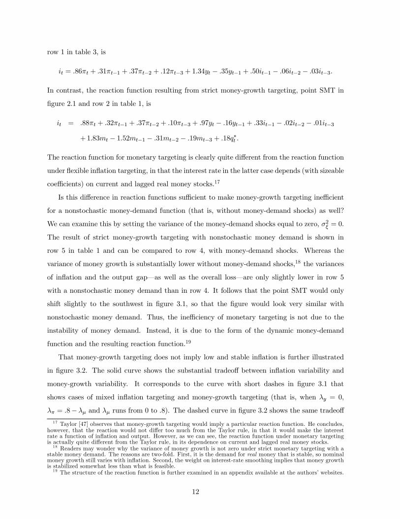
row 1 in table 3, is

it = :86¼t + :31¼t¡1 + :37¼t¡2 + :12¼t¡3 + 1:34yt ¡ :35yt¡1 + :50it¡1 ¡ :06it¡2 ¡ :03it¡3:

In contrast, the reaction function resulting from strict money-growth targeting, point SMT in

…gure 2.1 and row 2 in table 1, is

it = :88¼t + :32¼t¡1 + :37¼t¡2 + :10¼t¡3 + :97yt ¡ :16yt¡1 + :33it¡1 ¡ :02it¡2 ¡ :01it¡3+1:83mt ¡ 1:52mt¡1 ¡ :31mt¡2 ¡ :19mt¡3 + :18q¤t :

The reaction function for monetary targeting is clearly quite di¤erent from the reaction function

under ‡exible in‡ation targeting, in that the interest rate in the latter case depends (with sizeable

coe¢cients) on current and lagged real money stocks.17

Is this di¤erence in reaction functions su¢cient to make money-growth targeting ine¢cient

for a nonstochastic money-demand function (that is, without money-demand shocks) as well?

We can examine this by setting the variance of the money-demand shocks equal to zero, ¾2» = 0.

The result of strict money-growth targeting with nonstochastic money demand is shown in

row 5 in table 1 and can be compared to row 4, with money-demand shocks. Whereas the

variance of money growth is substantially lower without money-demand shocks,18 the variances

of in‡ation and the output gap—as well as the overall loss—are only slightly lower in row 5

with a nonstochastic money demand than in row 4. It follows that the point SMT would only

shift slightly to the southwest in …gure 3.1, so that the …gure would look very similar with

nonstochastic money demand. Thus, the ine¢ciency of monetary targeting is not due to the

instability of money demand. Instead, it is due to the form of the dynamic money-demand

function and the resulting reaction function.19

That money-growth targeting does not imply low and stable in‡ation is further illustrated

in …gure 3.2. The solid curve shows the substantial tradeo¤ between in‡ation variability and

money-growth variability. It corresponds to the curve with short dashes in …gure 3.1 that

shows cases of mixed in‡ation targeting and money-growth targeting (that is, when ¸y = 0,

¸¼ = :8¡ ¸¹ and ¸¹ runs from 0 to .8). The dashed curve in …gure 3.2 shows the same tradeo¤

17 Taylor [47] observes that money-growth targeting would imply a particular reaction function. He concludes,however, that the reaction would not di¤er too much from the Taylor rule, in that it would make the interestrate a function of in‡ation and output. However, as we can see, the reaction function under monetary targetingis actually quite di¤erent from the Taylor rule, in its dependence on current and lagged real money stocks.18 Readers may wonder why the variance of money growth is not zero under strict monetary targeting with a

stable money demand. The reasons are two-fold. First, it is the demand for real money that is stable, so nominalmoney growth still varies with in‡ation. Second, the weight on interest-rate smoothing implies that money growthis stabilized somewhat less than what is feasible.19 The structure of the reaction function is further examined in an appendix available at the authors’ websites.

12

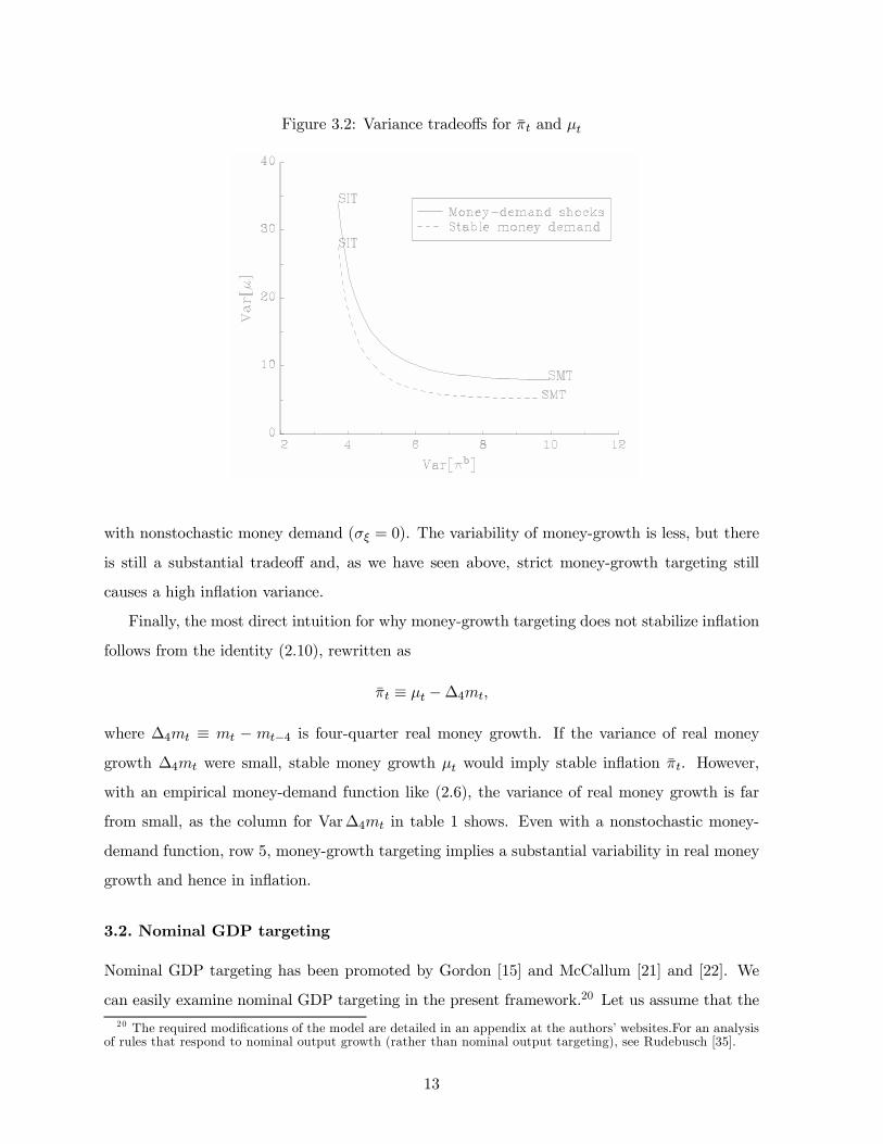
Figure 3.2: Variance tradeo¤s for ¹¼t and ¹t

with nonstochastic money demand (¾» = 0). The variability of money-growth is less, but there

is still a substantial tradeo¤ and, as we have seen above, strict money-growth targeting still

causes a high in‡ation variance.

Finally, the most direct intuition for why money-growth targeting does not stabilize in‡ation

follows from the identity (2.10), rewritten as

¹¼t ´ ¹t ¡¢4mt;

where ¢4mt ´ mt ¡ mt¡4 is four-quarter real money growth. If the variance of real moneygrowth ¢4mt were small, stable money growth ¹t would imply stable in‡ation ¹¼t. However,

with an empirical money-demand function like (2.6), the variance of real money growth is far

from small, as the column for Var¢4mt in table 1 shows. Even with a nonstochastic money-

demand function, row 5, money-growth targeting implies a substantial variability in real money

growth and hence in in‡ation.

3.2. Nominal GDP targeting

Nominal GDP targeting has been promoted by Gordon [15] and McCallum [21] and [22]. We

can easily examine nominal GDP targeting in the present framework.20 Let us assume that the20 The required modi…cations of the model are detailed in an appendix at the authors’ websites.For an analysis

of rules that respond to nominal output growth (rather than nominal output targeting), see Rudebusch [35].

13

relevant target variable is four-quarter nominal GDP growth, gt, de…ned as

gt ´ (pt + qt)¡ (pt¡4 + qt¡4) = ¹¼t + qt ¡ qt¡4: (3.1)

We can then add the term ¸gVar[gt] to the loss function (2.11), and represent nominal-GDP-

growth targeting (NGT) by ¸g = 0:8 and ¸¢i = 0:2.

The column for Var[gt] in table 1 reports the variance of nominal-GDP growth for all the

targeting cases. Row 6 reports the variances for nominal-GDP-growth targeting. Naturally, the

variance of nominal-GDP growth is then the lowest. We see that the variance of in‡ation is high,

and that the variance of the output gap is particularly high. The corresponding point NGT is

far to the right outside …gure 3.1.

Thus, nominal-GDP-growth targeting would be a very ine¢cient policy, even worse than

strict money-growth targeting. The reason for this ine¢ciency is apparently the one pointed out

by Ball [4] and further discussed in Svensson [43, Working Paper version], McCallum [23], Dennis

[9] and Guender [16]. Since monetary policy a¤ects output with a shorter lag than for in‡ation,

nominal-GDP growth can be stabilized by output adjustments at a relatively short horizon

when in‡ation is predetermined. These output adjustments, in turn, lead to high variability of

in‡ation, which then requires even higher output variability in order to stabilize nominal-GDP

growth. Only a positive weight on interest-rate smoothing prevents complete instability.

3.3. An alternative P* model of in‡ation

The model used above, which has no direct role for money in the determination of output or

in‡ation, does have the advantage of capturing to some approximation the views of many central

bankers, including those at the ECB. In particular, although the ECB has no current o¢cial

model, many researchers at the ECB and elsewhere use a model similar to the one above (e.g.,

Coenen and Wieland [6] and Peersman and Smets [33]).) As noted above, these views are shaped

by the data. It is very di¢cult to …nd signi…cant, stable, direct e¤ects of money on the economy.

For example, even over the short sample from 1961 to 1990, including several lags of quarterly

money growth make no signi…cant contribution to explaining in‡ation.

An alternative model with money that appears to have some empirical success is the P*

model of in‡ation of Hallman, Porter, and Small [17] (see Svensson [46] for a recent discussion):

¼t+1 = ~®¼1¼t + ~®¼2¼t¡1 + ~®¼3¼t¡2 + ~®¼4¼t¡3 ¡ ®p(pt ¡ p¤t ) + "t+1, (3.2)

14

where p¤t ´ mt+v¤t ¡q¤t is the long-run equilibrium price level and v¤t is the long-run equilibriumvalue of (log) velocity (that is, resulting from output equal to potential output and the interest

rate equal to its long-run equilibrium value). As noted above, for the 1960 to 1990 period in

the U.S., velocity is stationary, so v¤t is a constant, v¤. The rationale for the P ¤ model is that

in a stable long-run equilibrium where output grows at potential and velocity has stabilized at

its equilibrium, the quantity equation indicates that the aggregate price level must equal p¤t .

There are two transformations of the price gap that help illuminate the relationship of the

P* equation (3.2) to the Phillips curve (2.1). First, as noted in Hallman, Porter, and Small [17],

¡(pt¡p¤t ) = (qt¡q¤t )¡(vt¡v¤). Thus, if velocity remains fairly close to its long-run equilibriumvalue, the negative of price gap matches the output gap and the P* model reduces to a standard

Phillips curve in terms of the output gap. As shown in …gure 2.1, velocity remained relatively

close to its long-run average except during the 1990s. The 1990s therefore provide a test of the

relative value of the Phillips curve and P* models, and, as discussed below, it is a test that

the P* model fails. A second interesting transformation of the price gap (noted in Whitesell

[50] and Svensson [46]) is ¡(pt ¡ p¤t ) = mt ¡ q¤t + v¤ ´ mt ¡m¤t , where m¤t ´ q¤t ¡ v¤t is thelong-run equilibrium real money stock; that is, the negative of the price gap equals a real money

gap, mt ¡m¤t . Furthermore, note that in terms of an empirical regression analysis, since v¤ isa constant here, it is absorbed by the regression constant (or in our case by the de-meaning

of the regression variables) and so plays no role in explaining movements in in‡ation. Thus,

the empirical comparison between the Phillips curve and P* models depends on which quantity

gap better predicts in‡ation: the output gap between qt and q¤t (i.e., yt) or the real money

gap between mt and m¤t (in this case between mt and q¤t ). Any di¤erence between the two

models hinges on whether real output relative to potential or real money relative to (that same)

potential provides a better measure of the aggregate supply and demand imbalance that drives

in‡ation.

These two quantity gaps are shown in …gure 3.3. There is little quantitative di¤erence

between the output and real money gaps from 1961:Q1 to 1990:Q4—their correlation is .77 .

Not surprisingly then, the P* model performs similarly to the Phillips curve during this sample:

¼t+1 = :720¼t ¡ :065¼t¡1 + :265¼t¡2 + :080¼t¡3 + :077 (mt ¡m¤t ) + "t+1;(:091) (:111) (:111) (:089) (:020)

(3.3)

R̄2 = :82; SE = 1:064; DW = 1:98:

Indeed, at the crude aggregate level that we are working at and over this short sample, there is

15

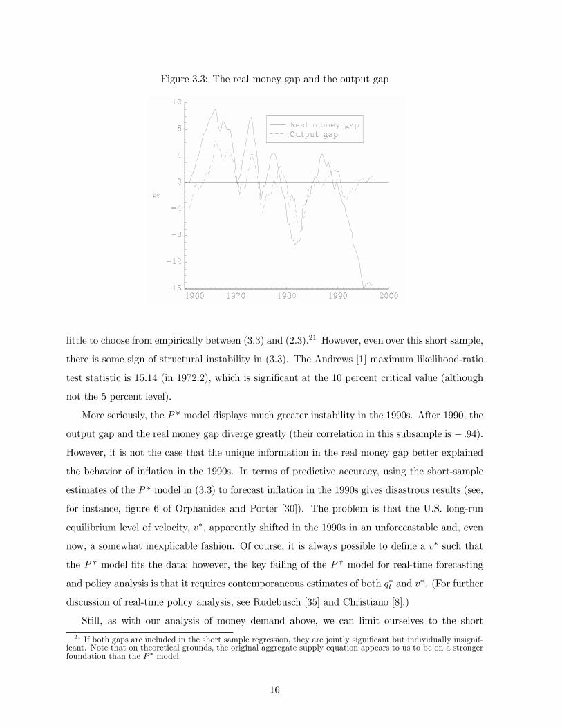
Figure 3.3: The real money gap and the output gap

little to choose from empirically between (3.3) and (2.3).21 However, even over this short sample,

there is some sign of structural instability in (3.3). The Andrews [1] maximum likelihood-ratio

test statistic is 15.14 (in 1972:2), which is signi…cant at the 10 percent critical value (although

not the 5 percent level).

More seriously, the P* model displays much greater instability in the 1990s. After 1990, the

output gap and the real money gap diverge greatly (their correlation in this subsample is ¡ :94).However, it is not the case that the unique information in the real money gap better explained

the behavior of in‡ation in the 1990s. In terms of predictive accuracy, using the short-sample

estimates of the P* model in (3.3) to forecast in‡ation in the 1990s gives disastrous results (see,

for instance, …gure 6 of Orphanides and Porter [30]). The problem is that the U.S. long-run

equilibrium level of velocity, v¤, apparently shifted in the 1990s in an unforecastable and, even

now, a somewhat inexplicable fashion. Of course, it is always possible to de…ne a v¤ such that

the P* model …ts the data; however, the key failing of the P* model for real-time forecasting

and policy analysis is that it requires contemporaneous estimates of both q¤t and v¤. (For further

discussion of real-time policy analysis, see Rudebusch [35] and Christiano [8].)

Still, as with our analysis of money demand above, we can limit ourselves to the short

21 If both gaps are included in the short sample regression, they are jointly signi…cant but individually insignif-icant. Note that on theoretical grounds, the original aggregate supply equation appears to us to be on a strongerfoundation than the P ¤ model.

16

sample where the P* model performs well. This system, which represents an extreme best case

scenario for supporting money targeting, comprises equations (3.3), (2.4), and (2.7). Despite the

substantial monetary character of this model, as shown in table 2, a positive weight on money-

growth stabilization results in an ine¢cient combination of in‡ation and output-gap variability,

also for a nonstochastic money demand.22

Table 2. Variances and losses in the P* modelCase ¸¼ ¸y ¸¹ ¸g Var ¹¼t Var yt Var¹t Var¢it Var¢4mt Var gt Loss1. FIT .4 .4 0 0 3.42 3.56 10.61 1.42 12.91 7.40 3.082. SMT 0 0 .8 0 19.26 16.43 2.95 4.36 20.95 16.93 15.153. SMTN 0 0 .8 0 16.22 14.44 0.41 1.39 15.42 14.38 12.54Note: For all cases, ¸¢i = :2: For case 3, SMTN refers to nonstochastic money demand, that is, ¾» = 0:

4. Lessons for the Eurosystem

4.1. A lesson about money-growth targeting

Above, we have shown in a simple empirical model that money-growth targeting can be quite

ine¢cient, in the sense of inducing overly variable in‡ation or output. As noted in the intro-

duction, the monetary policy strategy of the Eurosystem assigns a prominent role to money

growth. In particular, the deviation of current M3 growth from a reference value is interpreted

as an indicator of the risk to price stability. However, the Eurosystem has rejected monetary

targeting, by emphasizing that money growth will not be an intermediate target to be brought

in line with the reference value. Issing [20] is quite explicit on this:

[T]he monetary policy strategy selected by the ESCB is not a variant of intermediatemonetary targeting... Certain technical pre-conditions have to be met before a mon-etary targeting strategy is feasible. Speci…cally, an intermediate monetary targetwould only be a meaningful guide to monetary policy if a stable relationship existedbetween money and prices, and money was controllable in the short run using policydetermined interest rates...

Future shifts in the velocity of money are certainly possible—perhaps even likely.They cannot be predicted with certainty. Moreover, it is not clear whether thoseaggregates that have the best results in terms of stability are su¢ciently control-lable in the short-term with the policy instruments available to the ESCB. In thesecircumstances, relying on a pure monetary targeting strategy would constitute anunrealistic, and therefore misguided, commitment.

22 Gerlach and Svensson [14], although …nding substantial empirical support for the real money gap as apredictor of future in‡ation, also …nd that the Eurosystem’s nominal money-growth indicator is likely to be apoor indicator of future in‡ation.

17

Thus, according to Issing, the Eurosystem has rejected monetary targeting for the Eurosys-

tem, on the grounds that money demand is likely to be unstable and not su¢ciently controllable.

The implication seems to be that, if euro money demand had been found to be stable and su¢-

ciently controllable, money-growth targeting would have been appropriate. Furthermore, if the

Eurosystem would, in the future, …nd that money demand is stable and su¢ciently controllable,

money-growth targeting might be appropriate and the money-growth indicator might change

status and become an intermediate target variable.

The empirical demand function for U.S. M2 that we have estimated is quite well-behaved.

By excluding the period after 1991 from the sample, we obtain a relatively stable money-demand

function with a good …t and small money-demand shocks. Furthermore, money is quite control-

lable in this equation, with a semielasticity of one-quarter-ahead real and nominal money with

respect to the federal funds rate given by ·m·i = :135. Nevertheless, even with this well-behaved

money demand function, money-growth targeting would be very ine¢cient in the U.S. Even if

we were to set the money-demand shocks equal to zero and make the money-demand equation

completely nonstochastic, the e¢ciency of money-growth targeting would improve only slightly.

Similarly, if the euro-area economy can be reasonably well described by a system of equations

not too dissimilar from our model (as argued in the introduction), we must conclude that

money-growth targeting by the Eurosystem is likely to be quite ine¢cient, even under the

extreme assumption of a completely nonstochastic money demand. Thus, one main lesson for

the Eurosystem seems to be that it would be wise to continue rejecting money-growth targeting,

regardless of whether the demand for euro M3 is nonstochastic or not, and regardless of how

controllable it is.

4.2. A lesson about the money-growth indicator

Even though the Eurosystem has rejected money-growth targeting, it maintains that the money-

growth indicator is a crucial indicator for its price-stability-oriented monetary policy. Indeed,

since the money-growth indicator has been elevated to be one of the two “pillars” supporting

Eurosystem monetary policy, the impression is that the Eurosystem will give it at least the

same weight as its internal in‡ation forecasts. Svensson [44] and [45] has criticized the emphasis

on the money-growth indicator and argued that it is likely to be a poor indicator of the risk

to price stability. In e¤ect, on theoretical grounds, it appears to mainly be a noisy indicator

of current in‡ation, rather than a good predictor of future in‡ation at horizons relevant for

18

monetary policy decisions.

Can we say anything about the likely performance of the money-growth indicator from

the empirical model in the present paper? The issue boils down to how well money growth

predicts future in‡ation. We examine this by calculating the correlation between money growth

and two di¤erent in‡ation forecasts.23 First, we have the “unchanged-interest-rate” forecast of

four-quarter in‡ation T quarters ahead, denoted ¹¦t+T jt(it¡1). This is the forecast conditional

on an unchanged interest rate, it+¿ = it¡1 for ¿ ¸ 0, and the current state of the economy.

Svensson [44] argues that the best indicator of the risk to price stability is the deviation between

an unchanged-interest-rate forecast and the in‡ation target. This indicator obviously signals

by how much the in‡ation target is likely to be missed if there is no policy adjustment. It

also signals the direction and the magnitude of the optimal instrument adjustment. Then,

the correlation of current money growth with the unchanged-interest-rate forecast for di¤erent

horizons should be a good measure of the performance of the money-growth indicator. Second,

we have the “equilibrium” forecast of four-quarter in‡ation T quarters ahead, denoted ¹¼t+T jt.

This is the forecast conditional on the optimal reaction function (2.12) and the current state of

the economy.

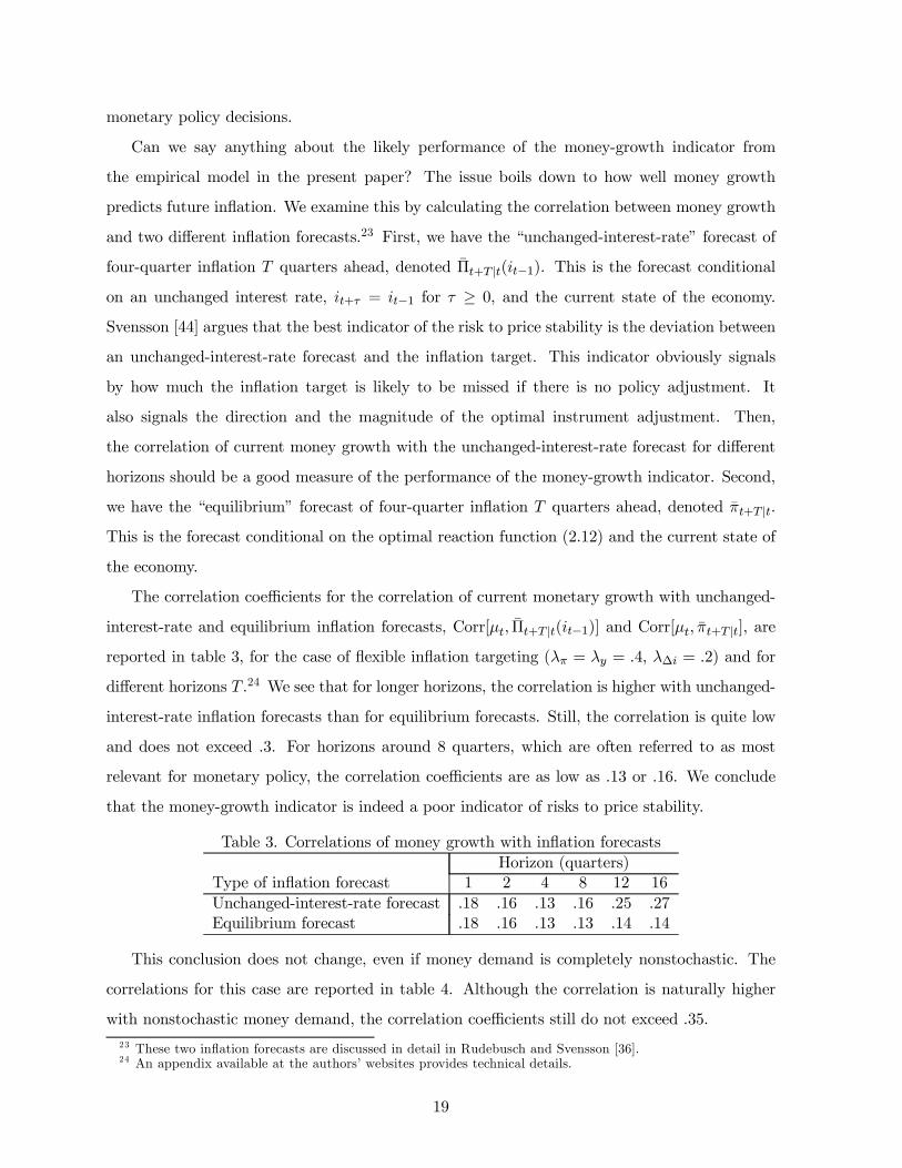
The correlation coe¢cients for the correlation of current monetary growth with unchanged-

interest-rate and equilibrium in‡ation forecasts, Corr[¹t; ¹¦t+T jt(it¡1)] and Corr[¹t; ¹¼t+T jt], are

reported in table 3, for the case of ‡exible in‡ation targeting (¸¼ = ¸y = :4, ¸¢i = :2) and for

di¤erent horizons T .24 We see that for longer horizons, the correlation is higher with unchanged-

interest-rate in‡ation forecasts than for equilibrium forecasts. Still, the correlation is quite low

and does not exceed .3. For horizons around 8 quarters, which are often referred to as most

relevant for monetary policy, the correlation coe¢cients are as low as .13 or .16. We conclude

that the money-growth indicator is indeed a poor indicator of risks to price stability.

Table 3. Correlations of money growth with in‡ation forecastsHorizon (quarters)

Type of in‡ation forecast 1 2 4 8 12 16Unchanged-interest-rate forecast .18 .16 .13 .16 .25 .27Equilibrium forecast .18 .16 .13 .13 .14 .14

This conclusion does not change, even if money demand is completely nonstochastic. The

correlations for this case are reported in table 4. Although the correlation is naturally higher

with nonstochastic money demand, the correlation coe¢cients still do not exceed .35.23 These two in‡ation forecasts are discussed in detail in Rudebusch and Svensson [36].24 An appendix available at the authors’ websites provides technical details.

19

Table 4. Correlations of money growth with in‡ation forecasts,nonstochastic money demand

Horizon (quarters)Type of in‡ation forecast 1 2 4 8 12 16Unchanged-interest-rate forecast .22 .20 .17 .20 .32 .33Equilibrium forecast .22 .20 .16 .16 .17 .18

Thus, with regard to the properties of money growth in the euro area, the main lesson is

that it is likely to be a rather inferior indicator of future in‡ation.

5. Conclusions

Using an empirical model of U.S. in‡ation, output and money, we compare the performance

of monetary targeting relative to in‡ation targeting. We exclude the period after 1990, when

M2 money demand displayed considerable instability, from the sample period for the money-

demand estimation. As a result, our estimated money-demand equation is quite well-behaved

with moderate money-demand shocks and controllable money demand.

Nevertheless, our results unambiguously show that monetary targeting would be quite inef-

…cient for the U.S., in the sense of bringing much higher variability of in‡ation and the output

gap than in‡ation targeting. Furthermore, setting money-demand shocks equal to zero and thus

assuming a completely nonstochastic money demand only marginally reduces the ine¢ciency of

monetary targeting.

Thus, counter to conventional wisdom, our results indicate that monetary targeting is not

mainly ine¢cient due to potential instability of money demand. Instead, the ine¢ciency of

monetary targeting is connected to the properties of the reaction function or the central bank’s

instrument following from monetary targeting. The dynamics of money demand is such that

the resulting reaction function is quite unsuitable for stabilizing in‡ation and the output gap,

even if there are no shocks to money demand.25 Thus, as argued on theoretical grounds in

Svensson [41], [42] and [44], the reasons for the poor performance of monetary targeting are

deeper and more fundamental than the instability of money demand. In terms of the identity

that in‡ation equals nominal money growth less real money growth, with an empirical money-

demand equation, nominal money-growth targeting does not stabilize real money growth and

25 Of course, we have only scratched the surface in terms of an analysis of monetary policy under uncertainty.However, the recent literature (for instance, Rudebusch [34] and Söderström [39]) suggest that introducing simpleparameter uncertainty (varying the coe¢cients within their standard error bands) has little e¤ect. In addition,with regard to uncertainty about the real-time data, Amato and Swanson [2] show that money data are alsosubject to important revisions. Thus, it is not obvious that monetary targeting would be favored with suchuncertainty.

20

hence not in‡ation.

The lessons for the Eurosystem are obvious. Fortunately, the Eurosystem has rejected mon-

etary targeting and emphasized that the deviation of money growth from the reference value

is to be used as an indicator of risks to price stability rather than as an intermediate target

variable. Nevertheless, the Eurosystem has given a prominent role to this indicator and elevated

it to the status of one of two pillars supporting its monetary policy, the other pillar being the

Eurosystem’s internal in‡ation forecast. There seems to be no support for that elevation of

the money-growth indicator. Our results indicate that the money-growth indicator has quite a

low correlation with in‡ation forecasts, both unchanged-interest-rate and equilibrium forecasts.

Therefore, money growth is likely to be a poor indicator of risks to price stability. This is even

more problematic since the Eurosystem has announced that it will keep its internal in‡ation

forecasts secret and use the money-growth indicator and the reference value as the main com-

municating device with the market and the general public. Instead of the money-growth being

one of two pillars, it should rather, at most, be one brick among many in the construction of

in‡ation and output–gap forecasts that will be the crucial input in its monetary policy decisions.

In passing, we have also shown that nominal-GDP targeting, in our empirical model of

the U.S. economy, would be an even more ine¢cient policy than monetary targeting. Since

monetary policy realistically a¤ects output with a shorter lag than for in‡ation, nominal-GDP

growth can be stabilized by output adjustments at a relatively short horizon, for which in‡ation

is predetermined. These output adjustments, in turn, lead to high variability of in‡ation, which

then requires even higher output variability in order to stabilize nominal-GDP growth.

21

References

[1] Andrews, Donald W.K. (1993), “Tests for Parameter Instability and Structural Change

with Unknown Change Point,” Econometrica, 61(4), 821–856.

[2] Amato, Je¤ery D. and Norman Swanson (1999), “The Real-Time (In)Signi…cance of

Money,” manuscript, Bank for International Settlements.

[3] Baba, Y., David Hendry, and Ross Starr (1992), “The Demand for M1 in the U.S.A.”

Review of Economic Studies 59, 25–61.

[4] Ball, Laurence (1997), “E¢cient Rules for Monetary Policy,” NBER Working Paper No.

5952.

[5] Browne, F.X., G. Fagan and J. Henry (1997), “Money Demand in EU Countries: A Survey,”

Sta¤ Paper No. 7, European Monetary Institute.

[6] Coenen, Günter, and Volker Wieland (2000), “A Small Estimated Euro Area Model with

Rational Expectations and Nominal Rigidities,” manuscript, European Central Bank.

[7] Congressional Budget O¢ce (1995), “CBO’s Method for Estimating Potential Output,”

CBO Memorandum, October 1995.

[8] Christiano, Lawrence J. (1989), “P* Is Not the In‡ation Forecaster’s Holy Grail,” Quarterly

Review 13, Federal Reserve Bank of Minneapolis, Fall, 3–18.

[9] Dennis, Richard (1998), “Instability Under Nominal GDP Targeting: The Role of Expec-

tations,” Working Paper, Australia National University.

[10] European Central Bank (1999), “Editorial,” ECB Monthly Bulletin, January 1999, 9–10.

[11] Estrella, Arturo, and Frederic S. Mishkin (1997), “Is there a Role for Monetary Aggregates

in the Conduct of Monetary Policy?” Journal of Monetary Economics 40, 279–304.

[12] Feldstein, Martin, and James H. Stock (1994), “The Use of a Monetary Aggregate to Target

Nominal GDP,” in N. Gregory Mankiw (ed.), Monetary Policy, University of Chicago Press

(Chicago), 7–62.

22

[13] Gerlach, Stefan, and Frank Smets (1995), “The Monetary Transmission Mechanism: Evi-

dence from the G-7 Countries,” in Financial Structure and the Monetary Policy Transmis-

sion Mechanism, Bank for International Settlements (Basle, Switzerland), 188–224.

[14] Gerlach, Stefan, and Lars E.O. Svensson (1999), “Money and In‡ation in the Euro Area:

A Case for Monetary Indicators?” Working Paper.

[15] Gordon, Robert J. (1985), “The Conduct of Monetary Policy,” in A. Ando, H. Eguchi, R.

Farmer and Y. Suzuki, eds., Monetary Policy in Our Times, MIT Press, Cambridge, MA,

45–81.

[16] Guender, Alfred V. (1998), “Nominal Income Targeting vs. Strict In‡ation Targeting: A

Comparison,” Working Paper, University of Canterbury, Christchurch.

[17] Hallman, Je¤rey J., Richard D. Porter, and David H. Small, (1991), “Is the Price Level

Tied to the M2 Monetary Aggregate in the Long Run?,” American Economic Review 81,

841–858.

[18] Hamburger, M. (1977), “Behavior of the Money Stock: Is There a Puzzle?,” Journal of

Monetary Economics 3, 265–288.

[19] Hess, Gregory D., Christopher S. Jones, and Richard D. Porter, (1998), “The Predictive

Failure of the Baba, Hendry, and Starr Model of M1,” Journal of Economics and Business

50, 477–507.

[20] Issing, Otmar (1998), “The European Central Bank at the eve of EMU,” speech in London,

November 26, 1998.

[21] McCallum, Bennett T. (1988), “Robustness Properties of a Rule for Monetary Policy,”

Carnegie-Rochester Conference Series on Public Policy 29, 173–204.

[22] McCallum, Bennett T. (1997), “Issues in the Design of Monetary Policy Rules,” NBER

Working Paper No. 6016.

[23] McCallum, Bennett T. (1997b), “The Alleged Instability of Nominal Income Targeting.”

NBER Working Paper No. 6291.

[24] Meltzer, Allan H. (1999), “The Transmission Process,” Working Paper, Carnegie-Mellon

University.

23

[25] Mehra, Yash P. (1997), “A Review of the Recent Behavoir of M2 Demand,” Federal Reserve

Bank of Richmond Economic Quarterly 83(3), 27–43.

[26] Meyer, Laurence H. (1997), “The Economic Outlook and Challenges for Monetary Policy,”

Remarks at the Charlotte Economics Club, Charlotte, North Carolina, January 16.

[27] Nelson, Edward (2000), “Direct E¤ects of Base Money on Aggregate Demand: Theory and

Evidence,” Working Paper, Bank of England.

[28] Oliner, Stephen D., and Glenn D. Rudebusch (1995), “Is There a Bank Lending Channel

for Monetary Policy,” Economic Review, Federal Reserve Bank of San Francisco, No. 2,

3–20.

[29] Oliner, Stephen D., Glenn D. Rudebusch, and Daniel Sichel (1996), “The Lucas Critique

Revisited: Assessing the Stability of Empirical Euler Equations for Investment,” Journal

of Econometrics 70, 291–316.

[30] Orphanides, Athanasios, and Richard Porter, (2000), “P* Revisited: Money-Based In‡ation

Forecasts with a Changing Equilibrium Velocity,” Journal of Economics and Business 52,

87–100.

[31] Porter, Richard, and David Small (1989), “Understanding the Behavior of M2 and V2,”

Federal Reserve Bulletin 75, 244–254.

[32] Reifschneider, David, Robert Tetlow, and John Williams (1999), “Aggregate Disturbances,

Monetary Policy, and the Macroeconomy: The FRB/US Perspective,” Federal Reserve

Bulletin 85, 1–19.

[33] Peersman, Gert, and Frank Smets (1999), “Uncertainty and the Taylor Rule in a Simple

Model of the Euro-Area Economy,” Working Paper.

[34] Rudebusch, Glenn D. (1999), “Is the Fed Too Timid? Monetary Policy in an Uncertain

World,” Working Paper 99-05, Federal Reserve Bank of San Francisco.

[35] Rudebusch, Glenn D. (2000), “Assessing Nominal Income Rules for Monetary Policy with

Model and Data Uncertainty,” Working Paper 2000-03, Federal Reserve Bank of San Fran-

cisco.

24

[36] Rudebusch, Glenn D., and Lars E.O. Svensson (1999), “Policy Rules for In‡ation Tar-

geting,” in Monetary Policy Rules, ed. by John B. Taylor, 203–246. Chicago: Chicago

University Press.

[37] Smets, Frank (1995), “Central Bank Macroeconometric Models and the Monetary Policy

Transmission Mechanism,” in Financial Structure and the Monetary Policy Transmission

Mechanism, Bank for International Settlements (Basle, Switzerland), 225–266.

[38] Smets, Frank (1999), “Output Gap Uncertainty: Does It Matter For the Taylor Rule?,”

In Monetary Policy under Uncertainty, eds. B. Hunt and A. Orr, pp. 10–29. Wellington:

Reserve Bank of New Zealand.

[39] Söderström, Ulf (1999), “Should Central Banks Be More Agressive?” Working Paper,

Stockholm School of Economics.

[40] Stock, James H., and Mark W. Watson (1999), “Forecasting In‡ation,” Journal of Monetary

Economics 44, 293–335.

[41] Svensson, Lars E.O. (1997), “In‡ation Forecast Targeting: Implementing and Monitoring

In‡ation Targets,” European Economic Review 41, 1111–1146.

[42] Svensson, Lars E.O. (1999a), “In‡ation Targeting as a Monetary Policy Rule,” Journal of

Monetary Economics 43, 607–654.

[43] Svensson, Lars E.O. (1999b), “In‡ation Targeting: Some Extensions,” Scandinavian Jour-

nal of Economics 101, 337–361.

[44] Svensson, Lars E.O. (1999c), “Monetary Policy Issues for the Eurosystem,” Carnegie-

Rochester Conference Series on Public Policy 51-1, 79–136.

[45] Svensson, Lars E.O. (1999d), “Price-Stability as Target for Monetary Policy: De…ning

and Maintaining Price Stability,” in Deutsche Bundesbank, The Monetary Transmission

Process: Recent Developments and Lessons for Europe, MacMillan, London, forthcoming.

[46] Svensson, Lars E.O. (2000), “Does the P ¤ Model Provide Any Rationale for Monetary

Targeting?” German Economic Review 1, 69–81.

[47] Taylor, John B. (1999a), “A Historical Analysis of Monetary Policy Rules”. in Taylor [48].

25

[48] Taylor, John B., ed. (1999b), Monetary Policy Rules, Chicago University Press.

[49] Taylor, John B. (1999c), “The Robustness and E¢ciency of Monetary Policy Rules as

Guidelines for Interest Rate Setting by the European Central Bank,” Journal of Monetary

Economics 43, 655–679.

[50] Whitesell, William, (1997), “Interest Rates and M2 in an Error Correction Macro Model,”

Federal Reserve Board, FEDS Working Paper 1997-59.

26

Eurosystem Monetary Targeting:Lessons from U.S. Data

Glenn D. Rudebusch and Lars E.O. Svensson

Unpublished Technical Appendices

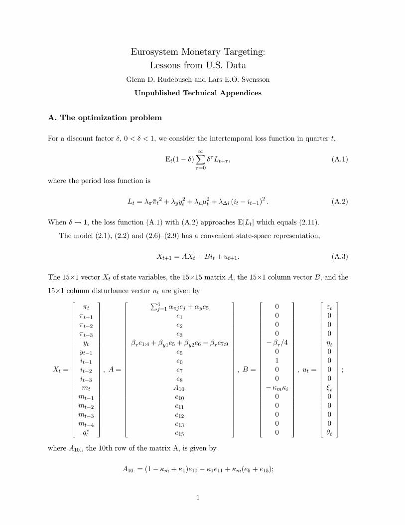
A. The optimization problem

For a discount factor ±, 0 < ± < 1, we consider the intertemporal loss function in quarter t,

Et(1¡ ±)1X¿=0

±¿Lt+¿ ; (A.1)

where the period loss function is

Lt = ¸¼¹¼t2 + ¸yy

2t + ¸¹¹

2t + ¸¢i (it ¡ it¡1)2 : (A.2)

When ± ! 1, the loss function (A.1) with (A.2) approaches E[Lt] which equals (2.11).

The model (2.1), (2.2) and (2.6)–(2.9) has a convenient state-space representation,

Xt+1 = AXt +Bit + ut+1: (A.3)

The 15£1 vector Xt of state variables, the 15£15 matrix A, the 15£1 column vector B, and the15£1 column disturbance vector ut are given by

Xt =

266666666666666666666666666664

¼t¼t¡1¼t¡2¼t¡3ytyt¡1it¡1it¡2it¡3mtmt¡1mt¡2mt¡3mt¡4q¤t

377777777777777777777777777775

; A =

266666666666666666666666666664

P4j=1 ®¼jej + ®ye5

e1e2e3

¯re1:4 + ¯y1e5 + ¯y2e6 ¡ ¯re7:9e5e0e7e8A10¢e10e11e12e13e15

377777777777777777777777777775

; B =

266666666666666666666666666664

0000

¡¯r=40100

¡·m·i00000

377777777777777777777777777775

; ut =

266666666666666666666666666664

"t000´t0000»t0000µt

377777777777777777777777777775

;

where A10:, the 10th row of the matrix A, is given by

A10¢ = (1¡ ·m + ·1)e10 ¡ ·1e11 + ·m(e5 + e15);

1

ej (j = 0; 1; :::; 15) denotes a 1£15 row vector, for j = 0 with all elements equal to zero, for

j = 1; :::; 15 with element j equal to unity and all other elements equal to zero; and where ej:k

(j < k) denotes a 1£15 row vector with elements j; j+1; :::; k equal to 14 and all other elements

equal to zero.

Furthermore, it is convenient to de…ne the 4£1 vector Yt of goal variables. It ful…lls

Yt = CXXt +Ciit; (A.4)

where the vector Yt, the 4£15 matrix CX and the 4£1 column vector Ci are given by

Yt =

26664¹¼tyt¹t

it ¡ it¡1

37775 ; CX =26664

e1:4e5

e1:4 + e10 ¡ e14¡ e7

37775 ; Ci =266640001

37775 :Then, the period loss function can be written

Lt = Y0tKYt; (A.5)

where the 4£4 matrix K has the diagonal (¸¼; ¸y; ¸¹; ¸¢i) and all its o¤-diagonal elements are

equal to zero.

With (A.3), (A.1) and (A.2), the problem is written in a form convenient for the standard

stochastic linear regulator problem (cf. Chow [1] and Sargent [2]). Minimizing (A.1) in each

quarter, subject to (A.3) and the current state of the economy, Xt, results in a linear feedback

rule for the instrument of the form (2.12). More precisely, the optimal instrument rule is the

vector f in (2.12) that ful…lls

f = ¡ ¡R+ ±B0V B¢¡1 ¡U 0 + ±B0V A¢ ;where the 15£ 15 matrix V ful…lls the Riccati equation

V = Q+ Uf + f 0U 0 + f 0Rf + ±M 0VM;

where M is the transition matrix given by (A.10) and Q, U and R are given by

Q = C0XKCX ; U = C0XKCi; R = C

0iKCi:

Furthermore, the optimal value of (A.1) is

(1¡ ±)X 0tVXt + ± trace (V§uu) ; (A.6)

2

where §uu = E [utu0t] is the covariance matrix of the disturbance vector. In the limit when ±

approaches 1, the optimal rule converges to the one minimizing (2.11) and the optimal value of

(2.11) is

E [Lt] = trace (V §uu) : (A.7)

For any reaction function of the form (2.12), the dynamics of the model follows

Xt+1 = MXt + ut+1 (A.8)

Yt = CXt; (A.9)

where the matrices M and C are given by

M = A+Bf (A.10)

C = CX +Cif: (A.11)

For any given reaction function f resulting in …nite unconditional variances of the goal

variables, the unconditional loss (2.11) ful…lls

E [Lt] = EhY0tKYt

i= trace (K§Y Y ) ; (A.12)

where §Y Y is the unconditional covariance matrix of the goal variables.26

The covariance matrix §Y Y for the goal variables is given by

§Y Y ´ E£YtY

0t

¤= C§XXC

0; (A.13)

where §XX is the unconditional covariance matrix of the state variables. The latter ful…lls the

matrix equation

§XX ´ E£XtX

0t

¤=M§XXM

0 +§uu: (A.14)

We can use the relations vec(A+B) = vec(A) + vec(B) and vec(ABC) = (C0 ­A) vec(B)on (A.14) (where vec(A) denotes the vector of stacked column vectors of the matrix A, and ­denotes the Kronecker product) which results in

vec (§XX) = vec¡M§XXM

0¢+ vec (§uu)= (M ­M) vec (§XX) + vec (§uu) :

Solving for vec (§XX) we get

vec (§XX) = [I ¡ (M ­M)]¡1 vec (§uu) : (A.15)26 The trace of a matrix A, trace(A), is the sum of the diagonal elements of A.

3

B. The P ¤ model

In the P ¤ model, the …rst row in matrix A, A1¢, is simply replaced by

A1¢ =4Xj=1

®¼jej + ®me10 ¡ ®me15.

All other equations remain the same.

C. Strict monetary targeting without interest-rate smoothing

Consider strict monetary targeting without interest-rate smoothing, ¸¹ = 1 and ¸¼ = ¸y =

¸¢i = 0. We realize that a …rst-order condition for a minimum of (A.1) is then simply

¹t+1jt = 0; (C.1)

where for any variable xt, xt+¿ jt denotes the expectation of xt+¿ conditional on the information

available in period t, that is, Xt and it. From (2.6) and (2.10), we get

¹t+1jt ´ mt+1jt ¡mt¡3 + ¹¼t+1jt= ¢mt+1jt +mt ¡mt¡3 + ¹¼t+1jt= ¡·m(mt ¡ qt + ·iit) + ·1¢mt +mt ¡mt¡3 + ¹¼t+1jt:

Combining this with (C.1), solving for it and using (2.1) gives

it =1

·m·i¹¼t+1jt +

1

·iqt ¡ 1

·imt +

·1·m·i

¢mt +1

·m·i(mt ¡mt¡3)

=1

4·m·i

0@¼t+1jt + 2Xj=0

¼t¡j

1A+ 1

·i(yt + q

¤t ) +

µ1 + ·1 ¡ ·m

·m·i

¶mt ¡ ·1

·m·imt¡1 ¡ 1

·m·imt¡3:

Using (2.1) and the empirical estimates, we get

it = 3:10¼t+1:71¼t¡1+2:38¼t¡2+ :21¼t¡3+1:08 yt+ :80 q¤t +11:08mt¡4:47mt¡1¡7:41mt¡3:

D. The correlation between in‡ation forecasts and the money-growth indicator

Let ¹¼t+T jt denote the “equilibrium” in‡ation forecast (of four-quarter in‡ation T quarters ahead),

that is, the forecast conditional on the optimal reaction function (2.12) and the current state of

the economy, Xt. By (A.8)–(A.11), it is given by

¹¼t+T jt = C1¢Xt+T jt = C1¢MTXt ´ aTXt;

4

where Cj¢ denotes the jth row of the matrix C.

Let ¹¦t+T jt(it¡1) denote the “unchanged-interest-rate” in‡ation forecast (of four-quarter in-

‡ation T ¸ 1 quarters ahead), that is, the forecast conditional on an unchanged interest rate,it+¿ = it¡1 for ¿ ¸ 0, and the current state of the economy, Xt. We note that

it¡1 = e7Xt

and de…ne

~M ´ A+Be7

~C ´ CX +Cie7:

Then the unchanged-interest-rate forecast is given by

¹¦t+T jt(it¡1) = ~C1¢Xt+T jt = ~C1¢ ~MTXt ´ ~aTXt:

Furthermore, in equilibrium we can write

¹t = C3¢Xt ´ bXt:

It follows that

Corr[¹¼t+T jt; ¹t] =Cov[¹¼t+T jt; ¹t]qVar[¹¼t+T jt] Var[¹t]

=aT§XXb

0qaT§XXa0T b§XXb0

:

Similarly,

Corr[¹¦t+T jt(it¡1); ¹t] =~aT§XXb

0q~aT§XX~a

0T b§XXb

0:

E. Nominal-GDP-growth targeting

Nominal-GDP-growth targeting requires expanding the vector of state variables by the four

variables qt¡1, qt¡2, qt¡3 and qt¡4. Then, the 19£1 vector Xt of state variables, the 19£19

5

matrix A, the 19£1 column vector B, and the 19£1 column disturbance vector ut are given by

Xt =

266666666666666666666666666666666666664

¼t¼t¡1¼t¡2¼t¡3ytyt¡1it¡1it¡2it¡3mtmt¡1mt¡2mt¡3mt¡4q¤tqt¡1qt¡2qt¡3qt¡4

377777777777777777777777777777777777775

; A =

266666666666666666666666666666666666664

P4j=1 ®¼jej + ®ye5

e1e2e3

¯re1:4 + ¯y1e5 + ¯y2e6 ¡ ¯re7:9e5e0e7e8A10¢e10e11e12e13e15

e5 + e15e16e17e18

377777777777777777777777777777777777775

; B =

266666666666666666666666666666666666664

0000

¡¯r=40100

¡·m·i000000000

377777777777777777777777777777777777775

; ut =

266666666666666666666666666666666666664

"t000´t0000»t0000µt0000

377777777777777777777777777777777777775

;

where ej and ej:k (j < k) now denotes 1£19 row vectors.Furthermore, the 5£1 vector Yt of goal variables, the 5£19 matrix CX and the 5£1 column

vector Ci are given by

Yt =

2666664¹¼tyt¹t

it ¡ it¡1gt

3777775 ; CX =2666664

e1:4e5

e1:4 + e10 ¡ e14¡ e7

e1:4 + e5 + e15 ¡ e19

3777775 ; Ci =266666400010

3777775 ;

and the 5£5 weight matrix K has the diagonal (¸¼; ¸y; ¸¹; ¸¢i; ¸g) and all its o¤-diagonal

elements are equal to zero.

References

[1] Chow, Gregory C. (1970), Analysis and Control of Dynamic Economic Systems, John Wiley

and Sons, New York.

[2] Sargent, Thomas L. (1987), Dynamic Macroeconomic Theory, Harvard University Press,

Cambridge MA.

6