European Ecosystem Assessment – Concept, Data, and ...
70
European Ecosystem Assessment – Concept, Data, and Implementation Contribution to Target 2 Action 5 Mapping and Assessment of Ecosystems and their Services (MAES) of the EU Biodiversity Strategy to 2020 Draft 04 March 2015 Photo: © Chadi Abi Faraj Prepared by / compiled by: Dania Abdul Malak Organisation: ETC/SIA EEA project manager: Markus Erhard
Transcript of European Ecosystem Assessment – Concept, Data, and ...

European Ecosystem Assessment – Concept, Data, and Implementation
Contribution to Target 2 Action 5 Mapping and Assessment of Ecosystems and their Services (MAES) of the EU Biodiversity
Strategy to 2020
Draft 04 March 2015
Photo: © Chadi Abi Faraj
Prepared by / compiled by: Dania Abdul Malak
Organisation: ETC/SIA
EEA project manager:
Markus Erhard

2 European Ecosystem Assessment Concept, Data, and Methodology
Contents
Acknowledgements
Summary
1 Introduction ........................................................................................... 7
1.1 Why ecosystem assessment ................................................................ 7
1.2 Policy background ................................................................................ 8
2 Concept ................................................................................................ 11
2.1 Ecosystems, habitats, and biodiversity ............................................ 11
2.2 Ecosystems, ecosystem services and natural capital ..................... 15
2.3 Framework for European ecosystem assessment ........................... 17
2.4 Data availability ................................................................................... 21
3 Implementation .................................................................................... 23
3.1 Mapping the pressures ....................................................................... 23
3.1.1 Drivers and pressures ........................................................................... 23
3.1.2 Mapping cumulative effects of pressures and trends ............................ 31
3.2 Mapping ecosystem conditions ......................................................... 36
3.2.1 Mapping ecosystem distribution ............................................................ 37
3.2.2 Mapping ecosystem conditions ............................................................. 43
3.2.3 Mapping multiple factors of condition and trends .................................. 46
4 Impacts and Response ....................................................................... 47
4.1 Impacts on ecosystem function, habitat quality and biodiversity .. 47
4.1.1 Functional traits of biodiversity .............................................................. 47
4.1.2 Impact assessment ............................................................................... 48
4.2 Link to Response ................................................................................ 49
5 Conclusions and outlook ................................................................... 50

European Ecosystem Assessment Concept, Data, and Methodology 3
List of Acronyms Acronyms Name
AQ Air Quality
BD Birds Directive
CAP Common Agricultural Policy
CBD Convention on Biological Diversity
CDDA Common Database on Designated Areas (nationally designated areas)
CCE Coordination Centre for Effects
CICES Common international classification of Ecosystem services
CIF Common Implementation Framework
CLC CORINE Land Cover
CORILIS CORINE Lissage
CORINE Coordination of Information on the Environment
CPUE Catch per unit effort
DEM Digital Elevation Model
DG Directorate General of the European Commission
DG-ENV Directorate General of the European Commission-Environment
DPSIR Drivers-Pressures-State-Impact-Response framework
EA Ecosystem assessment
EASIN European Alien Species Information Network
EC European Commission
ECRINS European catchments and Rivers network System
EEA European Environment Agency
EFFIS European Forest Fire Information System
EFI European forest institute
EFISCEN European Forest Information Scenario database
EMEP European Monitoring and Evaluation Programme
EMIS Environmental Marine Information System
ESPON European Observation Network for Territorial Development and Cohesion
ETC/BD European Topic Centre on Biodiversity
ETC/ICM European Topic Centre on Inland, Coastal and Marine waters
ETC/SIA European Topic Centre on Spatial Information and Analysis
EU European Union
EUNIS European Nature Information System
FAO Food and Agriculture Organization
FAO-AGA Food and Agriculture Organization's Animal Production and Health Division
FOEN Swiss Federal Office for the Environment
GAEC Good Agricultural and Environmental Condition
GFCM General Fisheries Council for the Mediterranean
HANTS Harmonic Analyses of NDVI Time-Series
HD Habitat Directive
HELCOM Baltic Marine Environment Protection Commission (Helsinki Commission)
HRL High Resolution Layers
HNV High Nature Value
IAS Invasive Alien species
ICES International council for exploration of the Sea
INSPIRE Infrastructure for Spatial Information in Europe
IUCN International Union for Conservation of Nature and Natural Resources
JRC Joint Research Centre
JRC CCM The Joint Research Centre Catchment Characterization and Modelling (CCM)
LEAC Land and Ecosystem Accounting

4 European Ecosystem Assessment Concept, Data, and Methodology
LRTAP Long-Range Transboundary Air Pollution
MA Millennium Ecosystem Assessment
MAES Mapping and Assessment of Ecosystems and their Services
MAES WG MAES Working Group
MCPFE Ministerial Conference on the Protection of Forests in Europe
MS Member States
MSFD Marine Strategy Framework Directive
NDVI Normalized Difference Vegetation Index
NEC National Emission Ceiling
OWL Other wooded land
RBD River Basin District
RUBICODE Rationalising Biodiversity Conservation in Dynamic Ecosystems
SEBI Streamlining European Biodiversity Indicators
TBFRA temperate and boreal forest resource assessment
TEEB The economics of Ecosystems and Biodiversity
UK NEA United Kingdom National Ecosystem Assessment
UN United Nations
UNECE United Nations Economic Commission for Europe
UWWTD Urban Waste Water Treatment Directive
VOC Volatile organic compounds
WFD Water Framework Directive
WISE Water Information System for Europe

European Ecosystem Assessment Concept, Data, and Methodology 5
Acknowledgements

6 European Ecosystem Assessment Concept, Data, and Methodology
Summary This report summarises EEA contributions to Target 2 Action 5 ‘Mapping and Assessment of Ecosystems and their Services (MAES)’ for the implementation of the EU Biodiversity Strategy to 2020 (EC, 2011), the Strategy of the EU to meet the global targets of the Convention of Biodiversity (CBD, 2010). Europe is becoming greener (Fuchs, et al. 2014) but, at the same time, losing biodiversity. At least one-out-of-three species in Europe is threatened with extinction (IUCN, 2011a-d). Many ecosystems are pushed towards the provision of one service – mainly food production, at the cost of the other services they usually provide. The EU Biodiversity Strategy to 2020 aims towards ‘healthy’ ecosystems that are rich in biodiversity and provide multiple services for human well-being.
Implementation is based on a common agreement between the EEA, the Commission Services (DG-ENV) and the Joint Research Centre (JRC), to share the work of European level assessment. As described in this report, the EEA is in the lead for mapping and assessing ecosystems and their conditions. The information, combined with the assessment of ecosystem services (JRC), will provide information about ecosystem conditions and their capacity to provide services on a European level.
First, the document provides an overview about the motivation to use an ecosystem-based approach, and the EU Biodiversity Strategy to 2020 as policy background.
The second chapter outlines specific aspects of addressing habitats and biodiversity in the context of ecosystems, ecosystem service assessments and natural capital, and describes the conceptual framework to map and assess ecosystems in more detail. It uses the DPSIR (Drivers Pressures State Impact Response) approach to put different elements of environmental information into coherent context. The Millennium Assessment (MA) identified a number of key drivers and pressures affecting ecosystems and their services that are essential for human well-being. For this study the pressures are grouped into five major blocks: habitat change, climate change, invasive species, land use management, and pollution and nutrient enrichment. These blocks reflect important processes affecting ecosystems at different scales (continental to local), and also the major policy lines to cope with negative effects. Finally, the major elements for mapping pressures, ecosystem conditions and impacts, are outlined and explained – followed by short summary of an extensive evaluation of existing European data.
In a third chapter, the mapping and assessment process is further explained. For each pressure, as well as for mapping and assessing ecosystem condition and its impacts on biodiversity, available data has been collected and summarised in a series of tables (Annex 2). The tables provide information about the mapping process, accessibility and the gaps identified. For each pressure, one example is shown, and data availability, as well as gaps, are addressed. Mapping ecosystem conditions comprises of two major building blocks. First, a European ecosystem map was produced by linking Corine land cover (CLC) data with the European Nature Information System (EUNIS) habitat information. This map includes the natural conditions of ecosystem types across Europe. Secondly, the actual ecosystem conditions have to be mapped by combining the ecosystem map with current environmental monitoring data and linking it to the maps describing the environmental pressures affecting ecosystems and biodiversity. To assess the impacts of pressures on ecosystem conditions and habitat quality and biodiversity, the functional relationships, i.e. the so-called functional traits, have to be evaluated and described. The knowledge about these relationships triggers the quality of the impact assessment. Each of these steps is illustrated – using cropland and grassland as examples. In parallel, methods on how to combine information to map cumulative pressures and conditions are outlined in flow charts.
Finally, the achievements of the European-wide ecosystem assessment are summarised, discussed, and set into context with the remaining challenges, for the provision of the relevant knowledge to underpin the quantitative targets of the EU Biodiversity Strategy to 2020 – mainly the ‘no net loss’ and the ‘restoration and prioritisation framework’. Further currently available data needs to be

European Ecosystem Assessment Concept, Data, and Methodology 7
integrated with the new data available (mainly) from European environmental legislation and monitoring.
1 Introduction 1.1 Why ecosystem assessment
Ecosystems are defined in the Convention on Biological Diversity (CBD) as ‘a dynamic complex of plant, animal and micro-organism communities and their non-living environment interacting as a functional unit’ (UN, 1992). Ecosystems are multi-functional. Each system provides a series of services for human well-being either directly, e.g. as food and fibre, or more indirectly by e.g. providing clean air and water. Ecosystem assessment is an instrument for structured and targeted analysis of environmental change and its impact on human well-being. The structural and functional entities of ecosystems are key entry points for our understanding of how species interact with each other and their abiotic environments, and how these interactions are affected by human activities.
Ecosystems contain a multitude of living organisms that have adapted to survive and reproduce in a particular physical and chemical environment. Anything that causes a change in the physico-chemical characteristics of the environment has the potential to change an ecosystems condition, its biodiversity and, consequently, its capacity to provide services. Any activity that removes or adds organisms can change the functionality of an ecosystem. An ecosystem assessment should evaluate all of the relevant factors affecting the ecosystem’s structure and function.
Spatially-explicit mapping is required to capture different gradients and variations of the relevant components, in space and time, affecting ecosystem function (Maes et al., 2014). The assessment of ecosystem condition provides information about its capability to continuously provide services for human well-being. This knowledge is essential to document the on-going loss and degradation of ecosystems and their services, the subsequent socio-economic impacts, and the identification of pathways towards sustainable development, in order to maintain the delivery of services. As such, ecosystem assessments provide the input for decision-making by addressing and integrating basic information to sectoral policies, i.e. mainly, territorial planning, nature protection, agriculture, forestry, freshwater, marine, climate change mitigation and adaptation, and air pollution reduction.
This report outlines the concepts and methods to map and assess ecosystems and their condition on a European level, and the main sources of data needed to map and assess ecosystems at the European scale. It highlights the major pressures on ecosystems and outlines the expected results. It is targeted to describe the functional relationships between ecosystem condition, the quality of its habitats, and its biodiversity. The approach is also feasible for use in other environmental sectors, such as water, agriculture or forest management. It aims to support European policies with European-wide harmonised information, provide the baseline for assessing ecosystem services, and support the work of Member States on their national assessments.
Box 1.1 Key terms and definitions (Maes, et al., 2013, updated)
Assessment: The analysis and review of information derived from research for the purposes of helping someone in a position of responsibility to evaluate possible actions, or to think about a problem. Assessment means assembling, summarising, organising, interpreting, and possibly reconciling pieces of existing knowledge and communicating them so that they are relevant and helpful to an intelligent but inexpert decision-maker (Parson, 1995).

8 European Ecosystem Assessment Concept, Data, and Methodology
Biodiversity: The variability among living organisms from all sources – including terrestrial, marine, and other aquatic ecosystems, and the ecological complexes of which they are part. Biodiversity includes diversity within species, between species, and between ecosystems (UN, 1992).
Drivers of change: Any natural or human-induced factor that directly or indirectly causes a change in an ecosystem. A direct driver of change unequivocally influences ecosystem processes and can therefore be identified and measured to differing degrees of accuracy; an indirect driver of change operates by altering the level or rate of change of one or more direct drivers (MA, 2005).
Ecosystems are defined in the Convention on Biological Diversity (CBD) as “a dynamic complex of plant, animal and micro-organism communities and their non-living environment interacting as a functional unit” (UN, 1992).
Ecosystem assessment: A social process through which the findings of science concerning the causes of ecosystem change, their consequences for human well-being, and management and policy options are brought to bear on the needs of decision-makers (UK NEA, 2011).
Ecosystem condition / Ecosystem state: The effective capacity of an ecosystem to provide services, relative to its potential capacity (MA, 2005). Capacity is triggered by the physical, chemical and biological condition of an ecosystem at a particular point in time, controlled by the natural condition and the anthropogenic pressures to which it is exposed.
Ecosystem function: Subset of the interactions between biophysical structures, biodiversity and ecosystem processes that underpin the capacity of an ecosystem to provide ecosystem services (TEEB, 2010).
Ecosystem service: The benefits that people obtain from ecosystems (MA, 2005). The direct and indirect contributions of ecosystems to human wellbeing (TEEB, 2010). The concept 'ecosystem goods and services' is synonymous with ecosystem services. The service flow in our conceptual framework refers to the service actually used.
Habitat: The physical location or type of environment in which an organism or biological population lives or occurs. Terrestrial or aquatic areas distinguished by geographic, abiotic and biotic features, whether entirely natural or semi-natural.
Indicator: An observed value – representative of a phenomenon to study. In general, indicators quantify information by aggregating different and multiple data. The resulting information is therefore synthesised.
Physico-chemical environment describes the physical and chemical conditions that control the existence and survival of species. Temperature, precipitation, humidity, soil structure and soil water content, slope, currents and flooding are important physical parameters. Chemical parameters are determined by soil chemical conditions, bedrock weathering, nutrient supply including fertilisation, and air and water pollution.
1.2 Policy background
In May 2011, the European Commission and Council adopted the ‘Communication for the Implementation of the Biodiversity Strategy to 2020’ (EC, 2011), which also implies the time lines to meet the Aichi targets of the Convention of Biodiversity (EC, 2014a). The headline target for 2020 is ‘halting the loss of biodiversity and the degradation of ecosystem services in the EU by 2020, and restoring them in so far as feasible, while stepping up the EU contribution to averting global biodiversity loss’. The Strategy translates this central objective into six specific targets, with 20 concrete actions to achieve them. The Common Implementation Framework (CIF) provides an overview of how these targets and actions are interlinked (see Fig. 1.2 below).
The concept and methodology of the ecosystem assessment described in this report is triggered by Action 5, of Target 2. It is implemented by the Working Group MAES (Mapping and Assessment of Ecosystems and their Services) – a joint body of the European Commission and Member States with

European Ecosystem Assessment Concept, Data, and Methodology 9
EEA participation. Action 5 states that ‘Member States, with the assistance of the Commission, will map and assess the state of ecosystems and their services in their national territory by 2014, assess the economic value of such services, and promote the integration of these values into accounting and reporting systems at EU and national level by 2020.’
The assessment and valuation of Action 5 is closely linked to the other actions of Target 2, i.e. Actions: 6a) Restoration and prioritisation framework, 6b) Green Infrastructure Strategy, 7a) Biodiversity proofing methodology and 7b) No Net Loss initiative. Links also need to be established to the other five Targets, i.e. 1) Conserving and restoring nature, 3) Sustainable agriculture and forestry, 4) Sustainable fishery, 5) Combatting invasive alien species, and 6) Addressing the global biodiversity crises. Giving an integrative view is important for use within decision-making processes and key to addressing synergies and trade-offs of policy impacts on ecosystems and their services.
The Strategy implies two timelines for their targets:
1. a medium term target: ‘by 2020, ecosystems and their services are maintained and enhanced by establishing green infrastructure and restoring at least 15 % of degraded ecosystems’;
2. a long-term target: ‘by 2050, European Union biodiversity and the ecosystem services it provides – its natural capital – are protected, valued and appropriately restored for biodiversity's intrinsic value and for their essential contribution to human wellbeing and economic prosperity, so that catastrophic changes caused by the loss of biodiversity are avoided’.
Figure 1.2 Common Implementation Framework (CIF) of the EU Biodiversity Strategy to 2020
Note: Since January 2014 Action 6a) and 6b) are merged and implemented as a joint working group on Green Infrastructure and Restoration.
Source: Maes, et al., 2013.

10 European Ecosystem Assessment Concept, Data, and Methodology
In September 2011, DG Environment (DG-ENV) of the European Commission, Eurostat, the Joint Research Centre (JRC) and the EEA, agreed to share the European-wide work for Action 5 in Target 2. The EEA committed to provide the building blocks to map and assess the condition of major ecosystems until 2014 – which is described in this report, i.e. steps 1 and 2 in Fig. 1.3 below. In parallel, the JRC will map and assess the defined ecosystem services, i.e. step 3 in Fig. 1.3.
Both organisations will closely cooperate to link and integrate activities based on an ecosystem, i.e. an ecosystem service-matrix approach as outlined in the RUBICODE project (Vandewalle et al., 2010). This information, combined with the assessment of ecosystem services by the JRC, will provide detailed information about the ecosystem condition and its capacity to provide services on a European level, i.e. step 4 in Fig. 1.3.
Figure 1.3 A common assessment framework for ecosystems and ecosystem services
Source: Maes, et al., 2014
Until 2020, alignment of ecosystem service assessments with scenarios of future changes and the valuations of ecosystem services for baselines and scenarios, will be integrated into environmental and economic accounting. Ecosystem assessments will provide the baselines for these activities.

European Ecosystem Assessment Concept, Data, and Methodology 11
2 Concept 2.1 Ecosystems, habitats, and biodiversity
Ecosystems, in more scientific terms, are communities of interacting organisms and the physical and chemical non-living components of their environment, e.g. water, mineral soil and climate. These biotic and abiotic components are linked together through food-webs, nutrient cycles and energy flows (Odum, 1971). Ecosystems provide general and specific habitats for typical and atypical communities of species or taxa – from the smallest single-cells to the largest multi-cellular organisms, and for all stages of their life cycles.
Box 2.1 Typology of ecosystems
Member States, together with DG-ENV, the JRC and the EEA, agreed on a list of European-wide ecosystem types feasible for the aggregation of national and local data and the dis-aggregation of European data – also reflecting main policy lines and environmental reporting. A detailed description is available in Maes, et al., (2013).
Major eco-system category (level 1)
Ecosystem type for mapping and assessment (level 2)
Description
Terrestrial Urban Urban ecosystems are areas where most of the human population lives. This class includes urban, industrial, commercial, and transport areas, urban green areas, mines, dumping and construction sites.
Cropland Croplands are the main food production areas including both intensively-managed ecosystems and multifunctional areas supporting many semi-natural and natural species along with food production (lower intensity management). It includes regularly or recently cultivated agricultural, horticultural and domestic habitats and agro-ecosystems with significant coverage of natural vegetation (agricultural mosaics).
Grassland Grasslands are areas covered by a mix of annual and perennial grass and herbaceous non-woody species – including tall forbs, mosses and lichens, with little or no tree cover. The two main types are managed pastures, semi-natural and natural (extensively managed) grasslands.
Forest and woodlands
Woodlands and forests are areas dominated by woody vegetation of various age, or they have succession climax vegetation types on most of the area, supporting many ecosystem services. Information on ecosystem structure, e.g. age group, species and diversity, is especially important for this ecosystem type.
Heathland and shrub
Heathlands and shrubs are areas with vegetation dominated by shrubs or dwarf shrubs. They are mostly secondary ecosystems with unfavourable natural conditions. They include moors, heathland and sclerophyllous vegetation.
Sparsely vegetated land
Sparsely vegetated lands often have extreme natural conditions that might support particular species. They include bare rocks, glaciers and dunes, beaches and sand plains.
Wetlands Inland wetlands are predominantly water-logged specific-plant and -animal communities that support water regulation and peat-related processes. This class includes natural or modified mires, bogs and fens, as well as peat extraction sites.
Fresh water Rivers and lakes
Rivers and lakes are the permanent freshwater inland surface waters. This class includes water courses and water bodies.
Marine* Marine inlets and transitional waters
Marine inlets and transitional waters are ecosystems on the land-water interface under the influence of tides and with salinity regimes higher than 0.5 ‰. They include coastal wetlands, lagoons, estuaries and other transitional waters, fjords and sea lochs as well as embayments.
Coastal The coastal ecosystems include coastal, shallow, and marine systems that experience significant land-based influences. These systems undergo diurnal fluctuations in temperature, salinity and turbidity, and are subject to wave disturbance. Depth is between 50m and 70 m.
Shelf The shelf refers to marine systems away from coastal influence and down to the shelf break. They experience more stable temperature and salinity regimes than coastal systems, and their seabed is below wave disturbance. They are usually about 200 m deep.
Open ocean The open ocean refers to marine systems beyond the shelf break with very stable temperature and salinity regimes particularly at the deep seabed. Depth is beyond 200 m.
*The current zonal classification refers to the reporting units of the Marine Strategy Framework Directive (MSFD) and might be replaced by a more ecosystem-based approach in the future.

12 European Ecosystem Assessment Concept, Data, and Methodology
Although this definition applies to all hierarchical levels – from a single water drop and its microorganisms, to Earth’s major vegetation zones (biomes), for the practical purposes of policy-relevant mapping and assessment at European level and, in view of the available information, ecosystems are considered here at the scale of land-cover-related units, e.g. urban, cropland, grassland, forests, rivers and lakes. These units represent the key elements for human management, e.g. in agriculture, forestry, fisheries and water management, to make the best use of their services. At the same time, this spatial scale also reflects the existing definitions of European environmental directives, namely the Habitats (HD), Birds (BD), Water Framework (WFD), and the Marine Strategy Framework Directive (MSFD).
Habitats, the space where an organism or ecological community normally lives or occurs, are linked to species or groups of species/communities and their requirements to the physico-chemical conditions of their environment. For the purposes of EUNIS, a ‘habitat’ is defined as: ‘a place where plants or animals normally live, characterized primarily by its physical features (topography, plant or animal physiognomy, soil characteristics, climate, water quality etc.) and secondarily by the species of plants and animals that live there’. Habitats are necessarily defined at a given scale. Some EUNIS habitats such as moss and lichen tundra or deep-sea mud may be of vast extent. Others such as cave entrances or springs, spring brooks and geysers are much smaller. Most but not all EUNIS habitats are in effect ‘biotopes’, that is to say ‘areas with particular environmental conditions that are sufficiently uniform to support a characteristic assemblage of organisms’. A few EUNIS habitats such as glaciers and highly artificial non-saline standing waters may be devoid of living organisms other than microbes. These features, although not strictly habitats, are included for completeness (Davies et al. 2004). As such, the definition includes both ecosystems and habitats in sensu stricto. Plant species and many insects, reptiles and amphibians may live in one specific ecosystem type, or in more specific habitats provided by explicit ecosystem structures and conditions. Dead wood in forests, for example, provide habitats for many insect species and are part of the forest structure, and thereby their habitats depend on how the forests are managed. Birds, fish, and mammals – especially predators at the high levels of the food web, often need clusters of ecosystems as habitats, at the scale of landscape/seascapes to cover their needs for living, feeding and reproduction. Consequently, habitats often do not match ‘one-on-one’ with ecosystem types.
Biodiversity implies all dimensions of living organisms (see Fig 2.1 below), which comprises of all species communities, i.e. of algae, plants and animals – from bacteria to big predators, including their: variety, i.e. species richness; number of individuals, i.e. abundance; genetic diversity. The abiotic factors triggering biodiversity are manifold. The main drivers of the presence or absence of species are light, temperature and water – including their short and long-term variations, all of which are summarised as ‘climatic conditions’, plus physical conditions including currents, chemical conditions, such as nitrogen, phosphorous concentrations or salinity, environmental heterogeneity, and disturbances (Pausas & Austin, 2001).
For Europe as a continent, three different aspects are important to steering biodiversity. First, there is a general gradient of increasing species richness at the cost of their abundance from North to South – a consequence of the climate and its changes over the last million years.
The second important aspect is human land and sea use and their management, which in most parts of Europe, has been in practice for many centuries or even millennia. Until the 19th century, human use of natural resources was nutrient and energy limited, and agricultural activities were based on managing small fields generating additional habitats for species in increasingly heterogeneous landscapes. This process is considered to have induced maximum biodiversity on European land about 200-300 years ago.
Many studies have found relationships between changes in species richness and nutrient availability (Kirkman et al., 2001). The typical response observed was a ‘humped-back curve’: species richness is low at low nutrient levels, increases to peak at intermediate levels and declines more gradually at high nutrient levels (Pausas & Austin, 2001). With industrialisation and its subsequent fast-growing human

European Ecosystem Assessment Concept, Data, and Methodology 13
population, from the mid-19th century onwards, the increasing availability of energy from fossil fuels, machinery, inorganic fertilisers and pesticides, and the average field size, nutrient availability and pollutant load, as well as indirect pressures such as landscape fragmentation, air and water pollution and climate change, increased. However, at the same time, landscape /seascape heterogeneity reduced and put increased pressures on species and their habitats. In parallel, increasing land-take for settlements, industry, infrastructures and mining use, reduces the area of natural ecosystems, fragments their extension and creates new urban ecosystems. This process accelerated over the last 40 years. The structure of the world’s ecosystems have changed more rapidly in the second half of the 20th century than at any time in recorded human history, and virtually all of Earth’s ecosystems have now been significantly transformed through human actions (MA, 2005).
Box 2.2 European land-use history and biodiversity ‘in a nutshell’
Pre-industrial, i.e. before mid-19th century:
- small fields and more areas for agriculture increased species habitats in European landscapes;
- extensive use and nutrient limitation fosters species diversity;
- use of renewable energy (wood, hydropower) and ‘constant’ climate keeps pressures limited;
- population growth is low and resource needs only slightly increasing.
Industrial after mid-19th century accelerating very much in second half 20th century:
- large fields and land abandonment reduced habitat diversity in European landscapes;
- intensive land use and the use of fertilisers and pesticides reduced species diversity;
- use of fossil fuels led to additional pressures by anthropogenic climate change and air pollution;
- population growth and increased average incomes increased pressures on land and sea by land-take and the use of natural resources.
Finally, the third important aspect for biodiversity is rareness. Due to special environmental conditions, or specific land use, habitats such as bogs, mires and inland heathlands are present as important elements of the European ecosystem types. The number of species in these ecosystems can be low in e.g. bogs and mires, but the value of these ecosystems is high because they only appear in a few areas and they are often of special importance for, e.g. migrating birds, or tourism. For their preservation, it is important to understand why these habitats exist, and how they should be managed and protected.
As outlined and illustrated in Figure 2.1 below, ecosystems, habitats and their biodiversity are closely linked to each other over scale and time. To understand how species interact with their environment and are affected by human use, and how these processes have changed over space and time, as well as the functional relationships between ecosystems, habitats and biodiversity, is key to making sound and profound decisions for their preservation. As further outlined in the following chapters, it requires information about the spatial distribution and extension of ecosystems and the different pressures affecting their conditions. Both vary over space and time and can be combined to assess the impacts on ecosystem services and biodiversity. The outcomes allow an outline of possible responses to be drawn on how to mitigate negative impacts, or adapt and change ecosystem management, to improve service provisions and biodiversity conditions.
Box 2.3 Ecosystems, biodiversity, and habitats in the context of European ecosystem assessment
The Convention on Biological Diversity (UN, 1992; Article 2. Use of Terms) defines:
Ecosystems

14 European Ecosystem Assessment Concept, Data, and Methodology
"Ecosystem" means a dynamic complex of plant, animal and micro-organism communities and their non-living environment interacting as a functional unit.
Habitats
"Habitat" means the place or type of site where an organism or population naturally occurs.
Biodiversity
"Biological diversity" means the variability among living organisms from all sources including, inter alia, terrestrial, marine and other aquatic ecosystems and the ecological complexes of which they are part; this includes diversity within species, between species and of ecosystems.
These definitions do not necessarily distinguish between the three entities. It makes it often difficult to address the causalities between human induced environmental change and environmental condition and its impacts on biodiversity and at the same time to offer options how to secure species presence and survival by improving the current environmental situation.
The ecosystem types as defined in MAES are linked to major sub-national, national and European policy lines such as agriculture, forestry, nature protection or territorial cohesion and address the sub-national to European scale. It implies that habitats are matching ecosystems one-on-one or are part of these ecosystems. Deadwood in forest ecosystems for example are important habitats for many insects but deadwood represents only one element in forest ecosystem structure and functioning. Ecosystems are also part of larger entities. Ecosystem functioning often depends on the location and spatial context and the relationships between ecosystems. Flood protection for example depends on the location, spatial distribution, and extension of the different ecosystem types and their capacity for water retention. Habitats e.g. for large mammals and birds often cover more than one ecosystem type for feeding and reproduction, requiring assessments on landscape scales.
Biodiversity implies all dimensions of living organisms, which comprises of all species communities, i.e. of algae, plants and animals – from bacteria to big predators, including their variety, i.e. species richness; number of individuals, i.e. abundance; genetic diversity. In context of MAES ecosystem assessment, its spatial and temporal scale, and the data available for assessments, the focus is on species richness and abundance which also implies genetic diversity even if not assessed explicitly in this context. Biodiversity is linked to quality of the habitats species occupy and as such is linked to ecosystem condition. Protecting and managing ecosystems affects their condition which is the key entry point for measures to improve habitat quality and subsequent biodiversity.

European Ecosystem Assessment Concept, Data, and Methodology 15
Figure 2.1 Biodiversity, habitats and ecosystems
Source: ETC/SIA 2014a
2.2 Ecosystems, ecosystem services and natural capital
Ecosystem services are defined as the benefits that people obtain from ecosystems (MA, 2005) contributing to human wellbeing (TEEB, 2010). The condition of ecosystems describes their effective capacity to provide these services. This is equivalent to actual ecosystem service capacity. The effective use of ecosystem services depends on the demands, which, again, depend on social and economic factors and their distribution over space and time. Urban areas depend, notably, on ecosystem services for drinking water, clean air, food, flood protection, temperature regulation and recreation. Cities largely rely on their hinterland, which leads to very high demands for a wide variety of ecosystem services in these areas – from food and water provisions to recreation, whereas the demand for services in rural areas can be rather low and may even be ‘exported’ to urban areas. Remote areas can provide numerous services that are important for the maintenance and regulation of our environment, but are not necessarily facing the same demand as urban periphery areas. The analytical framework of the MAES Working Group (MAES, et al., 2013), illustrates the link between ecosystems, their biodiversity, their function, and their services (Fig. 2.3). Ecosystem condition is not only affected by human use and management, but also by the use of the non-living parts of natural capital which include abiotic components such as mineral resources, fossil fuels, land/sea take for settlements, industry and infrastructures – including land/sea areas used to produce renewable energy (Fig. 2.4). Whilst the use of abiotic components does not rely on current ecosystem service capacity, the use of these abiotic components affects ecosystems directly by removing them – thus, taking them out of service, and indirectly increasing stress on ecosystems functional capacities by air pollution, nutrient load and anthropogenic climate change, i.e. the consequences of using minerals and fossil fuels.

16 European Ecosystem Assessment Concept, Data, and Methodology
Figure 2.3 Conceptual framework for EU-wide ecosystem assessment and its link to
ecosystem services.
Note: The blue box frames the content of the ecosystem assessment described in this report Source: Maes, et al., 2013
Figure 2.4 Link between ecosystems, ecosystem services and natural capital
Source: Petersen & Gocheva, 2015
Abiotic assets:
Solar radiation
Minerals, fossil fuels,ozone layer,
gravel,etc.
Natural capital
Abiotic flows:
Renewable energy (solar, wind, hydro..)
Phosphate fertiliser, radiation
protection,etc.
Ecosystems as asset:
Extent, structure & condition of :
Forests, woodlands, rivers, lakes, oceans,
coasts, wetlands, grasslands, croplands,
heathlands, urban parks, etc.
Ecosystem service flows:
• Provisioning services (food, fibre, energy etc.)
• Regulation & maintenance (of climate, river flow, pollination etc.)
• Cultural services (recreation in nature, spiritual use of nature etc.)
Ecosystem capital:
GENERATING

European Ecosystem Assessment Concept, Data, and Methodology 17
Many ecosystems are managed to maximise the provision of one service at the cost of other services – mostly for food, often timber. The EU Biodiversity Strategy to 2020 aims towards ‘healthy’ ecosystems’, which are rich in biodiversity and provide multiple services for human well-being. Safeguarding healthy, functioning ecosystems to deliver the range of ecosystem services required to meet the demands of our societies, guarantees that the condition of the environment, society and economy all work together and remain in good condition.
Reaching equilibrium between sustaining enough natural capital to deliver nature’s ecosystem services, while supporting the demands of a growing global population, is a major challenge worldwide – not just in Europe. If properly managed, ecosystems provide multiple services that are vital to humanity, including the production of: goods, e.g. food; life-support processes, e.g., water purification; life-fulfilling conditions, e.g., recreation opportunities; conservation of options, e.g. genetic diversity for future use. So far, only a limited number of these services – mainly provisioning and some of the cultural services such as recreation, are quantified and valued, i.e. accounted. Most of these services are handled as ‘free’ public goods. Assessing the economic value of such services, and promoting the integration of these values into accounting and reporting systems at EU and national levels, will be the next steps in the implementation process of the EU Biodiversity Strategy to 2020.
2.3 Framework for European ecosystem assessment
Ecosystems contain a multitude of living organisms that have adapted to life in a particular physico-chemical environment. Anything that causes change in the physico-chemical characteristics of the environment has the potential to change the ecosystem and affect its habitats and biodiversity. Additionally, any activity that removes or adds organisms can change the ecosystem too.
Data and information for the assessment of the current environmental conditions, environmental changes, as well as the impacts and (policy) responses to cope with negative impacts, can be structured using the well-established Drivers, Pressures, State, Impact and Response (DPSIR) framework (Niemeijer and de Groot, 2008).
DPSIR is a theoretical framework used to systematically classify the information needed for the analysis of environmental problems, on the one hand, and to identify measures to resolve them, on the other hand (Turner, 2010). Drivers of change (D) exert pressures (P) on the state /condition of ecosystems (S) at one moment of time, impacting habitats and biodiversity (I) across Europe in all combinations of intensities, and consequently affecting the amount of services they can provide. If these impacts are undesired, policy-makers will put in place the relevant responses (R) by taking actions to tackle negative effects. See Box 2.3 below.
The DPSIR framework is independent from spatial and temporal scales and can be adapted and applied to any ecosystem type at any level of detail. It supports the structuring of the approach and helps to identify the relevant data needed to perform assessment in adequate temporal and spatial resolutions.

18 European Ecosystem Assessment Concept, Data, and Methodology
Box 2.3 The DPSIR Framework for the European ecosystem assessment
There is not always full clarity about the exact definition of environmental processes and where to place the different components in the DPSIR framework – it also depends on the objects to be addressed. In some cases, pressures in the context of a specific ecosystem assessment, e.g. terrestrial, might be considered as a condition in a different context, e.g. freshwater, or vice versa.
In any case, the contextual linkages should be visible and the DPSIR framework should help to put these linkages in the right place. In many cases, knowledge and data availability may determine which element of the DPSIR framework is used to describe the impacts to be investigated. Finally, the impact as the target of the assessment – in our case, the impacts of environmental change on biodiversity, triggers the overall design of the assessment.
Note: For ‘state’, the report uses the term ‘condition’ to avoid confusion with the term ‘status’ that describes the legal aspects
Source: Turner et al., 2010 adapted
The Millennium assessment (see Box 2.4 below), does not distinguish between drivers and pressures but uses the terms ‘indirect drivers’ and ‘drivers’ instead (Nelson, 2005). To adapt the terminology to the DPSIR framework applicable for the European policy framework, these drivers are labelled as pressures and conditions that can be grouped into 2 major blocks:
1. The natural, physical, chemical, and biological conditions triggered by, climate, soil conditions and topography, and also by evolution, extreme events and other environmental pressures. Within the time horizon of the Biodiversity Strategy-related ecosystem assessment, which covers years – to several decades, the natural drivers of the Millennium Assessment are considered to be constant and are, therefore, part of natural conditions in the MAES DPSIR framework.
2. The pressures that ecosystems are exposed to –due to human use, are translated into five major blocks, i.e. habitat change, climate change (including inherent natural climate variations and extreme events), invasive species, land use management, and pollution and nutrient enrichment. Human pressures are either direct, i.e. mainly from land use and management, or indirect, i.e. by air pollution or anthropogenic climate change.
Drivers agriculture, forestry, water management, settlement, transport, industry, tourism, etc
Pressurespollution, nutrient load, fragmentation, climate
change, land takeintensification, exploitation,
invasive species
State ecosystem state and quality / structure and functioning
nutrient conditionhabitat diversity, species abundance and diversity
Impactschange/loss of ecosystem
functionchange/loss of biodiversity
Responsemaintaining ecosystem
functioning and biodiversitymanagement change, prevention measures,
protection, nutrient, pollution reduction

European Ecosystem Assessment Concept, Data, and Methodology 19
Box 2.4: Pressures in MAES ecosystem assessment and drivers in Millennium Assessment
The pressures have been pooled into 5 major groups each representing main policy
DPSIR MAES ecosystem
assessment
Drivers Millennium Assessment
Comment
Pressure habitat change changes in local land use and cover
Territorial cohesion: structural changes, land-take, fragmentation, land abandonment
Pressure climate change climate change Climate change mitigation and adaptation: changes in average values and extreme events (mainly temperature, precipitation, humidity)
Pressure alien species species introduction or removal Nature protection and EU Regulation on Invasive Alien Species (Oct 2014)
Pressure land-use / exploitation
harvest and resource consumption & technology, adaptation and use
CAP, Forestry: agricultural (including grazing) and forestry statistics – technological aspects are addressed, indirectly, via changes in land management, and the use of fertilisers and pesticides
Pressure pollution and nutrient enrichment
external inputs, e.g. fertiliser use, pest control and irrigation
Air pollution prevention, CAP, Nature protection: air pollution data, statistical data on fertiliser use, nutrients and pesticides
Condition natural conditions (ecosystem map)
natural, physical, and biological drivers
Current climate, soil conditions, elevation, slope, aspect, etc. considered stable within time horizon of the assessment (years to decades)
The main pressures identified also reflect major policy lines but often feed also into different policy measures. Land cover change is mostly object of territorial cohesion policies. Climate change is linked to climate change mitigation and adaptation policies. Land-use and nutrient enrichment are part of agricultural and forestry related policies but also affect nature protection and air pollution mitigation. To address the relevant stakeholders, this requires a clear communication strategy and appropriate thematic mapping of pressures and subsequent ecosystem conditions.
Another important factor for mapping and addressing ecosystems and their condition is the change of pressures over time. The cumulative effects of observed changes in pressures are the reason for the current conditions of ecosystems. It describes the trends in pressures that ecosystems have been exposed to, so far. Time-series of observed changes in pressures are, therefore, important to analyse the causal connectivity between pressures and current condition for each ecosystem type and each spatial unit across Europe. The trend in pressures also provides a first insight into the expected changes in the near future. Decreasing observed trends may indicate further improvement of ecosystem conditions and vice versa, i.e. important information for decision-making about measures to mitigate and adapt to positive or negative effects. Consequently, ecosystem assessments always imply information on observed trends in the pressures that created the current conditions and trigger those in the near future. For the implementation of the EU Biodiversity Strategy to 2020, ecosystem assessments are focused on the functional relationships between ecosystem conditions, their service capacities, their habitat quality and related biodiversity. Taking into account existing and upcoming data and information, on a European level, as well as the targets defined in the Strategy, a European-wide ecosystem assessment requires – as illustrated in Figure 2.5 below:
1. Spatially-explicit mapping of the key pressures of change in the direct pressures, e.g. land/sea use and management, harvesting, and land cover change, and indirect pressures, e.g. air

20 European Ecosystem Assessment Concept, Data, and Methodology
pollution, eutrophication and climate change, and their different gradients and variations in space and time – altering the condition of ecosystems and consequently impacting their service capacities, habitat qualities, and biodiversity across Europe;
2. Spatially-explicit mapping of ecosystems to define their location and boundaries and assess their natural capacities – since no pan-European ecosystem map is currently available;
3. Combination of data sets to assess the current condition of European ecosystems, which also includes change-over-time pressures to identify if trends lead to less or more favourable conditions in terms of their habitat qualities and biodiversity, functioning, and their capacity to provide services.;
4. Collection of profound and, if possible, quantitative information about the functional relationships between ecosystem conditions, service capacities, habitat qualities and their biodiversity;
5. Mapping impacts on ecosystem functions, habitats and biodiversity to provide information to meet the EU Biodiversity Strategy to 2020 targets and the related global Aichi targets of the Convention on Biological Diversity (CBD) (EC, 2014a).
The outcomes of the ecosystem assessment will feed into the subsequent assessment of their services and will provide input for valuing natural capital – as required in Communication (EC, 2011).
Figure 2.5 Main Building blocks for mapping and assessment of ecosystem condition and the impacts on biodiversity
Note: Ecosystem services, response and drivers are not object of this assessment – see Section 1.2
The interlinkages between different pressures, their relative importance for ecosystem condition, and the impacts on habitat quality and biodiversity, create a relative complex pattern of mutual interactions as illustrated in Fig. 2.6 below.
The relevance of the pressures depends on the ecosystem type. While crop- and grasslands used for agriculture ecosystems are mostly influenced by direct management, semi-natural systems such as heathlands and shrubs are more affected by air pollution and climate change. Freshwater and marine ecosystems are additionally impaired by the condition of adjacent terrestrial ecosystems and the input of nutrients and pollutants of these systems into the water bodies.
Pressure mapsChap. 3.1
Land/seacover maps
EUNIS dataSpecies and Habitat data
Ecosystem map(natural conditions)
Chap 3.2.1
Ecosystem condition maps
Chap. 3.2.2
Mapping and Assessment of
Ecosystem Services
(Policy) Response
Drivers
Impact mapsChap. 4.1.2
Functional Traits
Chap. 4.1.1
Data on ConditionChap. 3.2.1
Demand for human well-
being

European Ecosystem Assessment Concept, Data, and Methodology 21
Figure 2.6 Illustration of linkages between pressure, and the condition of ecosystems.
Note: Each main pressure is represented by one of several pressure indicators. Less important links are not presented for clarity
Source: ETC/SIA 2014a
2.4 Data availability
The implementation of the conceptual framework is triggered by the data available to assess and map pressures, ecosystem conditions, and impacts on their functional capacity across Europe for land, freshwater and marine areas. The assessment requires integration of a wide range of information – namely, spatial datasets, indicators, and statistics, and addresses different environmental sectors, including air quality, climate change, land cover, land/sea use, agriculture, forestry, water and marine, and nature protection. Additionally, reference data, e.g. climate, elevation and soil, are also needed in addition to the data of other sources, namely from earth observation tools and modelling. The categories of information to be integrated include:
data attributed to main land/sea cover and land/sea use classes, such as, disaggregated statistical and other not geo-referenced information;
up-scaled extrapolated, generalised local studies and experiments;
process-based modelling results and extrapolated point measurements;
quantitative and qualitative relationships between environmental pressures and ecosystem condition (indicators) and vice versa;
expert-based quantitative and qualitative assessments mainly on the level of impacts of major pressures on ecosystem function..
Data sets usually have to be linked in order to produce indicators that, in their combination, provide information on the pressures affecting ecosystem conditions. The main types of data to use in the assessment are listed in Table 2.1.
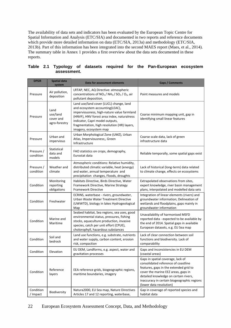
22 European Ecosystem Assessment Concept, Data, and Methodology
The availability of data sets and indicators has been evaluated by the European Topic Centre for Spatial Information and Analysis (ETC/SIA) and documented in two reports and reference documents which provide more detailed information on data (ETC/SIA, 2013a) and methodology (ETC/SIA, 2013b). Part of this information has been integrated into the second MAES report (Maes, et al., 2014). The summary table in Annex 1 provides a first overview about the data sets documented in these reports.
Table 2.1 Typology of datasets required for the Pan-European ecosystem assessment.
DPSIR Spatial data system
Data for assessment elements Gaps / Comments
Pressure Air pollution, deposition
LRTAP, NEC, AQ Directive: atmospheric concentrations of NO2 / NH3 / SO2 / O3, air pollutant deposition,
Point measures and models
Pressure
Land use/land cover and agro‐forestry
Land use/land cover (LUCL) change, land and ecosystem accounting(LEAC), imperviousness, high‐nature value farmland (HNVF), HNV forest area index, naturalness indicator, Capri model outputs, fragmentation, high resolution (HR) layers, imagery, ecosystem map
Coarse minimum mapping unit, gap in identifying small linear features
Pressure Urban and impervious
Urban Morphological Zone (UMZ), Urban Atlas, Imperviousness;, Green Infrastructure
Coarse scale data, lack of green infrastructure data
Pressure / condition
Statistical data and models
FAO statistics on crops, demography, Eurostat data
Reliable temporally, some spatial gaps exist
Pressure / condition
Weather and climate
Atmospheric conditions: Relative humidity, distributed climatic variable, heat (energy) and water, annual temperature and precipitation changes, Floods, droughts
Lack of historical (long‐term) data related to climate change, effects on ecosystems
Condition Monitoring reporting obligations
Habitats Directive, Birds Directive, Water Framework Directive, Marine Strategy Framework Directive
Extrapolated observations from sites, expert knowledge, river basin management plans, interpolated and modelled data sets
Condition Freshwater
ECRINS, waterbase ‐ rivers, groundwater, Urban Waste Water Treatment Directive (UWWTD), biology in lakes Hydrogeological Map
Integration of linear elements (rivers) and groundwater information; Delineation of wetlands and floodplains, gaps mainly in groundwater information
Condition Marine and Maritime
Seabed habitat, Sea regions, sea uses, good environmental status, pressures, fishing stocks, aquaculture production, invasive species, catch per unit effort (CPUE), cholorophyll, hazardous substances
Unavailability of harmonised MSFD reported data ‐ expected to be available by the end of 2014. Spatial gaps in available European datasets, e.g. EU Sea map
Condition Soil and bedrock
Land use functions, e.g. substrate, nutrients and water supply, carbon content, erosion risk, compaction
Lack of clear connection between soil functions and biodiversity. Lack of comparability
Condition Elevation EU DEM, Landforms, e.g. aspect, water and gravitation processes
Gaps and inconsistencies in EU DEM (coastal areas)
Condition Reference layers
EEA reference grids, biogeographic regions, maritime boundaries, imagery
Gaps in spatial coverage, lack of consolidated reference of coastline features, gaps in the extended grid to cover the marine EEZ areas, gaps in detailed knowledge on certain rivers, inaccuracy in certain biogeographic regions (lower data resolution)
Condition / Impact
Biodiversity Natura2000, EU Sea map, Nature Directives Articles 17 and 12 reporting, waterbase,
Gap in coverage of reported species and habitat data

European Ecosystem Assessment Concept, Data, and Methodology 23
nationally designated areas (CDDA), Red lists of species, European Nature Information system (EUNIS), habitat types, species assemblages, forest map, Morphological Spatial Pattern Analysis (MSPA), fragmentation, high‐nature value farmland and forest area, invasive species
New data from environmental reporting schemes, published in 2015, will complement current information – in terms of improving the current baseline of information, as well as allowing assessments of trends. The new State of Nature report of the Nature Directives, and the second water basin management reporting cycle of the Water Framework Directive (WFD), will be available and may allow a first assessment of how biodiversity of terrestrial and freshwater ecosystems and ecological status of water bodies changes over time. The first baseline report of the Marine Strategy Framework Directive (MSFD) will be available in 2015, providing an approach on how to assess ecosystems in the marine environment. The new Copernicus continental land service data (Corine 2012, thematic High Resolution Layers 2012) will provide both data on trends in land cover change (Corine land cover update, new high resolution layers for imperviousness and forest), and first data sets for water bodies, wetlands and grassland. The update of the SEBI 2010 (EEA 2010a) together with the other environmental indicators as listed in EEA (2013), and the forest ecosystem assessment report, are other important sources for the implementation of ecosystem assessments on a European level.
3 Implementation In the following chapters, an overview of the current state of mapping pressures, conditions, and impacts on ecosystems is provided together with one thematic map per main pressure and condition as an example. It illustrates how the concept can be implemented but cannot deliver a complete picture about available data for mapping and assessment.
3.1 Mapping the pressures
3.1.1 Drivers and pressures
Drivers induce pressures that affect the health of ecosystems, their biodiversity and, consequently, the ecosystem services they provide for human well-being at different spatial and temporal scales. This makes both their assessment and their management complex. Climate change may operate on a global or a large regional spatial scale; political change may operate at the scale of a nation or a municipal district. Socio-cultural change, inducing pressure change, typically occurs slowly on a time scale of decades – although abrupt changes can sometimes occur, i.e. in the case of wars or political regime changes, while economic changes tend to occur more rapidly.
As a result of these spatial and temporal dependences of drivers, the pressures that appear to be most significant, at a particular location and time, may not be the most significant over larger (or smaller) regions or time scales. The pressures exerted impact ecosystems and their biodiversity differently. Some pressures are widespread, e.g. air and water pollution that can affect ecosystems and their habitats over thousands of kilometres from their sources, e.g. acid rain, and eutrophication. Other pressures, such as overgrazing, agricultural intensification and timber extractions, have more local impacts, e.g. local, partial, or total loss of biodiversity. A variety of factors put pressures on ecosystems and their biodiversity, and most of these factors can be traced directly or indirectly to human activity. The effects of human activity seriously alter many basic ecosystem functions. These

24 European Ecosystem Assessment Concept, Data, and Methodology
pressures are exerted differently on different ecosystem types. For each driver, a series of datasets are identified to be included in the development of indicators on pressures.
Table 3.1 provides a list of pressures caused by the major drivers of ecosystem change and affecting ecosystem types. In Europe, land-take, land fragmentation and land use changes are direct pressures affecting all types of ecosystems – whereas other pressures are specific to certain ecosystems, e.g. the building of dams in rivers blocking water flow, or deep-sea resource exploitation in marine ecosystems.
Table 3.1 Pressures of ecosystem change they exert on biodiversity.
Ecosystem type
Major pressures of ecosystem change
Habitat changes Climate change
Invasive alien species
Land/sea use or exploitation
Pollution and nutrient enrichment
Urban Land‐take, landscape fragmentation due to urban sprawl and roads around cities, channelling of rivers in urban areas
Extreme events: droughts, floods, fires, heat waves, sea‐level rise in coastal cities
Expansion of alien species, introduction of exotic species in gardens
Non‐intensive use of land due to low density populations and jobs, lack of appropriate management of recreation areas, gravel extraction around cities, over‐exploitation of extraction of groundwater resource and freshwater
Contaminated soil by heavy metal due to industrial activities, air pollution and critical level of ozone, pollution of water when dysfunction of waste water management plan, sludge and waste
Cropland Land‐take, landscape fragmentation, agricultural intensification (structural changes)
Changes in monthly temperature and precipitation, extreme events, fires
Expansion of invasive alien species
Agriculture intensification, Loss in cropland productivity, abandonment
Fertilisers and pesticides, critical levels of ozone, nutrient enrichment
Grassland Landscape fragmentation, land abandonment, land‐take, habitat loss
Changes in monthly temperature and precipitation, extreme events, fires
Expansion of invasive alien species
Agricultural intensification, (over‐)harvesting, high irrigated land use, overgrazing, abandonment
Fertilisers, nutrient run‐off, critical levels of ozone, heavy metals
Woodland and forests
Land‐use change: conversion to agriculture, urbanisation, changes in forest pattern, fragmentation due to roads, land use changes ‐ forest isolation, land‐take
Changes in monthly temperature and precipitation, fires, extreme events, drought, frost, fires, floods, storms
Fast‐growing invasive alien species, e.g. Phytophthora disease
(Over‐)exploitation of timber and non‐wood products, felling, recreation and tourism, game hunting and (over‐)grazing
Nitrogen enrichment, heavy metals, air pollution and environmental contamination, eutrophication and acidification, ozone, critical levels of ozone
Heathland and shrub
Land‐use change, landscape fragmentation, land‐take, land abandonment
Extreme events, fires
Fast‐growing invasive alien species, e.g. Phytophthora disease
Lack of appropriate site management, recreational & urban disturbance
Nitrogen enrichment, critical levels of ozone, water drainage, heavy metals
Sparsely vegetated n/a n/a n/a n/a n/a

European Ecosystem Assessment Concept, Data, and Methodology 25
land
Wetland Land‐take, fragmentation, drainage for agriculture, reed harvest
Extreme events, drought, floods, changes in rainfall
Introduction of invasive predatory fishes, non‐predatory fish, plant species as Hydrocotyle ranunculoides and Azolla filiculoides
Blocking and extraction of water inflow, over‐exploitation of groundwater resources, (over‐)fishing, water extraction, reed harvest –for biofuels, helofytenfilter
Eutrophication, pesticides, acid rain, heavy metals, critical levels of ozone, plastic
Rivers and lakes
Modification of water courses, channelling, river regulation regimes, fragmentation (dams)
Changes in monthly temperature and precipitation, extreme events, drought
Invasive alien fish farm species
Water extraction, overfishing, fish farms, gravel extraction
Pollution, acid rain
Marine ecosystems: marine inlets and transitional waters, coastal, shelf, and open ocean
Coastal land‐take (tourism development)
Sea (surface) temperature Sea level rise
Expansion of invasive alien species
Offshore activities, over‐fishing, exploitation of oil and gas, aquaculture production
Eutrophication, heavy metals, fertilisers and pesticides, chemical pollution from industries and shipping
Source: ETC-SIA, 2013b
From the five major groups of pressures, habitat change is the pressure causing direct degradation or loss of ecosystems and habitats at local levels. It primarily aims to address land cover change-related processes. Habitat change is considered the major cause of biodiversity loss, leading to total or partial destruction or removal of habitats and replacement by other habitat types (land-cover change). It also decreases habitat quality by increasing soil erosion and soil degradation, as well as land abandonment, which also replaces habitats and, consequently, further impacts biodiversity. In addition, ecosystem changes modify the structure and function of habitats, which increase the vulnerability of populations of plants and animals to local extinction – due to hampered migration and dispersal because of destruction, fragmentation or degradation of their habitats. The main drivers of habitat degradation and loss are land-take. Around half of Europe’s land area is farmed, most forests are exploited, and natural areas are increasingly fragmented by other land use, i.e. mainly urbanisation and infrastructural development (EEA, 2010b).
Most of the relevant information for developing pressure indicators is available to support the development of ecosystem-specific indicators of the change in the extensions of ecosystems and the changes in conservation status of species and habitats. The most important data set for habitat-related pressures at the European level is the operational CORINE land-cover monitoring system for terrestrial ecosystems, which provides regular information about changes in land cover / land use including ecosystem size. Copernicus High Resolution Layers will provide more-detailed information on the changes in some land-cover classes, e.g. imperviousness and forest, and will improve the

26 European Ecosystem Assessment Concept, Data, and Methodology
baseline for monitoring grassland, wetlands, water bodies and riparian areas1. In parallel, the information on trends in habitat quality from Art.17 of the Habitat Directive provides important information – which is not specific on structural changes only, but also covers a full spectrum of pressures for a selection of species and habitats. For terrestrial fragmentation, only a baseline data set and no change detection is currently available, which limits the assessment of fragmentation as pressure. Phenological data and indirect indicators such, loss in soil production by land cover change, or pests and diseases, provide more information on habitat change.
For freshwater data on dams and measures to increase flow rates in rivers, are the main source of information of habitat fragmentation and loss. Apart from freshwater dam data, other data especially for construction and regulation measures in river beds is currently limited.
Marine sea use for energy production, aquaculture, mining and the use of sediments, are important pressures on water and seabed habitats, which currently not mapped systematically for assessments on a European level.
An overview of the available data sets is listed in Annex 2a. Map. 3.1 shows how fragmentation by infrastructure and other human-made barriers affect ecosystem structure and function across Europe
Map 3.1 Landscape fragmentation per 1 x 1 km2 grid from human-made barriers for the year 2009.
Note: Data is missing for Iceland, the Balkan countries, Turkey, the Azores and Madeira.
Source: EEA/FOEN 2011
1 http://land.copernicus.eu/pan-european

European Ecosystem Assessment Concept, Data, and Methodology 27
Climate is an integrated part of natural conditions and, thus, directly, or indirectly, affects all dimensions of biodiversity. The second major pressure – anthropogenic climate change, causes changes in the life-cycles of many European plants and animals, including frog and fish spawning, bird nesting, the arrival of migrant birds and butterflies and earlier spring phytoplankton blooms, pushing them to move northwards and uphill (EEA, 2012). It also creates risks of decoupling food-webs and changes in predator - prey interactions. Extreme events, such as floods, droughts, and fires, also change the health and characteristics of habitats and species.
Several indicators are available from various European institutes and projects, but the quality of the indicators is heterogeneous, especially for describing changes over time. Another issue is the quantitative attribution of observed climate change to its impacts on habitats and species. The ESPON Climate project has developed a series of climate change indicators (ESPON climate, 2011). The indicators of regional sensitivity to climate change provide information about the levels of: environmental sensitivity, e.g. protected natural areas, soil organic carbon content, and the propensity of soil erosion and forest fires; economic sensitivity, e.g. climate sensitive economic sectors namely forestry, agriculture, tourism, and energy production; physical sensitivity , e.g. settlements, roads, railways, airports, harbours, refineries, and thermal power plants; social sensitivity, e.g. location, age group distribution, density and size of urban areas.
As ecosystem assessments currently address mainly impacts on biodiversity, the use of the ESPON climate indicator developed on environmental sensitivity of European regions to climate change, can be used in the assessments of terrestrial and freshwater ecosystems (Map 3.2). For certain ecosystems, additional information is available to produce ecosystem-specific indicators, such as the European Forest Fire Information System (EFFIS) database of the JRC2 that provides observed temporal series on forest fire densities. Fire is not only linked to climate change but also partly, to natural conditions, especially in the Mediterranean area, and is often induced by direct human impact. Other important data sets are coastal storms, floods and droughts as listed in Annex 2b. Floods are important for both terrestrial ecosystems, mainly riparian areas, and the freshwater bodies. For marine ecosystems, sea surface temperature and acidification are important climate change-related pressures to consider in the assessment.
Another approach to assess climate change impacts would be the direct use of climate data (EEA 2012). In this case, it requires separate sensitivity analyses of habitats and biodiversity for temperature, precipitation and humidity impacts, in their various combinations, for changes in average and extreme events in time. EEA is hosting and maintaining an overall list of currently 46 indicators related to climate change and its impacts on terrestrial, freshwater and marine ecosystems (EEA, 2013). It also includes impacts on cryosphere soil and covers aspects such as plant and fungi phenology, species interactions, and water requirements for irrigation.
2 http://forest.jrc.ec.europa.eu/effis/about-effis/technical-background/european-fire-database/

28 European Ecosystem Assessment Concept, Data, and Methodology
Map 3.2 Environmental sensitivity to climate change in Europe
Source: ESPON Climate, 2011
Invasive alien species replace native species occupying their habitats, often degraded, leading to change in their survival and abundance. Invasive alien species may drive local native species to extinction via competitive exclusion, niche displacement, or hybridisation with related native species.
Therefore, alien species invasions may result in extensive changes in the structure, composition and global distribution of the biota with severe impacts on habitats, leading ultimately to the homogenisation of fauna and flora and the loss of biodiversity. This pressure affects all ecosystem types in Europe.
At the European level, Chytrý, et al., (2009), developed a map estimating the level of invasion of alien plants in Europe. The level of potential invasion of plant species can be seen in Map 3.3 below. It is based on observed alien species in vegetation plots distributed over different habitats. This information was extrapolated by relating it to the respective CORINE land cover classes that are favourable for the alien species. This information is relevant for use as a risk assessment map of invasions from alien plant species in Europe.
The map shows that the predicted level of invasion is different across Europe and assigns high predictions in the temperate zone of Western and central Europe, mainly in agricultural and urbanised areas. Since the assessment is based on number of alien species only not considering their abundance, individual neophytic species, which are extremely successful occupying new habitats are not well represented in this map. More information will be available due to the reporting scheme of the recently established EU Regulation on Invasive Alien Species, (EC, 2014b), (see Annex 2c).

European Ecosystem Assessment Concept, Data, and Methodology 29
Map 3.3 European map estimating the level of invasion by alien plant species
Source: Chytrý, et al., 2009
Land use, or exploitation, indicates the use of ecosystems mainly for the production of food and fibre. The intensity of land use by management has already severely-impacted habitat quality and biodiversity. Together with habitat change, it is the most important pressure on biodiversity mostly triggered by local management. Overexploitation is the result of unsustainable management practices that lead to irreversible depletion of natural resources, and is a major threat for biodiversity. It includes overgrazing grasslands, overharvesting forest ecosystems, and overfishing freshwater and marine ecosystems.
There is quite a variety of information accessible to map the pressures on ecosystems resulting from human management activities (Annex 2d). A good amount of information is available to address terrestrial ecosystems, especially the use of croplands, grasslands, and woodlands. It comprises of all harvesting data (agricultural and forest statistics), and land use /land management-related pressures such as irrigation and processes affecting soil quality. Map 3.4 provides an example of a composite indicator using yield statistics and nitrogen fertilization as proxy to assess intensity of land use for croplands.
So far no adequate data seems to be available for freshwater, on a European level, which would mainly include fishing, navigation, irrigation, water collection or energy production.

30 European Ecosystem Assessment Concept, Data, and Methodology
Information available to assess overfishing in European Seas is still scarce, as it is reported using different methods for different European sea regions. The use of available information is explored in a study on fish accounts (EEA work in progress).
Map 3.4 Land management intensity of croplands derived from crop statistics and related nitrogen application
Source ETC/SIA 2014a
Pollution and nutrient enrichment implies two main lines of pressures. First, there are direct effects, mainly by agricultural and forest-related land use, and management effects comprising of fertiliser, manure and pesticide inputs for production, varying at local scales. The second major pressure is the intake of nutrients and pollution, air pollution, and deposition, with effects on regional and continental scales. Damages occur when excessively harmful components are introduced into an ecosystem, exceeding the capacity of the ecosystem to maintain its natural balance and, particularly, the effects of inputs of nutrients, pesticides, microbes, industrial chemicals, metals and pharmaceutical products which ultimately end up in the soil, or in ground water and surface water (MA, 2005, EEA, 2010b). Pollution and nutrient enrichment change the characteristics of soils, thereby changing the biodiversity, i.e. habitats and species, causing biodiversity loss and ecosystem dysfunction, altered plant and animal communities, loss of species, and other harmful ecosystem changes.
Map 3.5 shows the exceedance of critical loads for eutrophication due to the deposition of nitrogen for the years 2000 and 2010, using the CSI indicator 005 (EEA, 2013). It can be used to assess the pressures on ecosystems from long-range air pollution. The critical load of the nutrient is defined as 'the highest deposition of nitrogen as NOx and/or NHy, below which, harmful effects in ecosystem structure and function do not occur – according to present knowledge'. Statistical data for fertilizer and pesticide input, which are closely linked to land use pressures, as well as data for other air pollutants are available for mapping.

European Ecosystem Assessment Concept, Data, and Methodology 31
For freshwater and marine ecosystems, data for point sources are available from the Urban Waste Water Treatment Directive (UWWTD). Nutrient and pollution from non-point sources requires modelling of the very complex interrelationships between freshwater bodies and surrounding terrestrial ecosystems. Therefore, this pressure is assessed by water quality monitoring which is linked to conditions as described further below.
For marine ecosystems, additional data describing pollution from accidents (oil spills) and marine litter disposals are available. Information is summarised in Annex 2e.
Map 3.5 Exceedance of nutrient critical loads for eutrophication due to the deposition of nitrogen for the year 2000 (right) and 2010 (left)
Source: CCE - EEA 2010 SEBI indicator 009
Source: CCE-EEA, 2015
3.1.2 Mapping cumulative effects of pressures and trends
Different spatial and temporal gradients of main pressures – each represented by a number of indicators, result in a complex pattern of factors affecting ecosystems, their habitats and biodiversity. As outlined, the pressures can be mapped and assessed individually to reflect potential measures and policy lines, such as nature protection, agriculture, forestry and territorial cohesion.
Pressures of the same type, with the same units, can be simply added-up as shown in map 3.6 (below) for agro-ecosystems, i.e. cropland and grassland used for agriculture, even if the calculation of individual pressures is rather complex. In this case, nitrogen input was derived from the nutrient accounts (ETC/SIA 2013b). The total nitrogen input to agricultural soils includes intentionally applied fertilisers (organic or mineral), manures from grazing livestock, biological nitrogen-fixation and atmospheric deposition.

32 European Ecosystem Assessment Concept, Data, and Methodology
Map 3.6 Total nitrogen input to agro-ecosystems (cropland and grassland) for the year 2010
Source: ETC/SIA 2014a
Ecosystem assessment in general should provide information about changes over time, because it is very important to know the observed trend that led to the current condition, the baseline for decisions on measures to mitigate future trends.
If sufficient data is available, time series of observed trends of pressures can be mapped – as already indicated in map 3.5 for critical loads of nitrogen, which allows spatially-explicit interpretations of the current conditions of ecosystems and expected trends in the near future. Map 3.7 provides an overview on the changing trends in nitrogen input in cropland and grassland ecosystems as average changes over 2000-2005, compared to the reference year 2000. The local patterns of changes with positive and negative trends in close neighbourhood (e.g. Po valley in Italy or Galicia region in Spain), illustrates the importance of spatially- explicit mapping and assessment.

European Ecosystem Assessment Concept, Data, and Methodology 33
Map 3.7 Trends in average Nitrogen inputs for the period 2000-2005 compared to the year 2000
Source: ETC/SIA 2014a
A second option is to combine pressures with different dimensions to show the cumulative effects and their variations across Europe. In this case, the values have to be re-scaled and combined either by summing up, equally weighting, or weighting individual pressures according to their relative importance for ecosystem functioning. The method can be applied to map any combination of pressures, independent from their gradient and number, but only qualitatively at the cost of quantitative assessments. This assessment option requires the involvement of mostly regional expertise in the weighting process to be assigned for the individual pressures depending on their relative contribution to the cumulative effects of pressures on ecosystems. Figure 3.1 illustrates the approach (flow) chart of how to perform the assessment.

34 European Ecosystem Assessment Concept, Data, and Methodology
Figure 3.1 General approach used for the development of single pressure and cumulative pressure indicators based on input datasets to assess the major pressures affecting ecosystems under each driver of change
Source: ETC/SIA 2014a

European Ecosystem Assessment Concept, Data, and Methodology 35
Map 3.8 below, provides an example of mapping cumulative pressures induced by land management for the ecosystem type ‘cropland’. The basic assumption for indicator development is that arable cropping is only beneficial to biodiversity when it is implemented by low intensity management.
To assess the intensity of arable land management, two main aspects are considered:
the “input” side (M1) of the management practices reflected by the use of fertilisers, the variety of crops and irrigation;
the “output” side (M2) represented by the yield produced on a particular area of land.
The arable crop index developed by the JRC (Paracchini & Britz, 2010), comprises of two aspects – fertiliser input and diversity of crops, in one indicator. To measure farmland management intensities, the arable crop index uses the sum of manure and mineral nitrogen applied per hectare. Crop diversity contributes to the indicator with the assumption that the richer the crop composition and the more equal the shares, the better for biodiversity. The index ranges from 0 (highly-intensive management, e.g. mono-cultures and high fertiliser use), to 100 (biodiversity-friendly management, e.g. rich crop diversity and little fertiliser use). The arable crop index is then further combined with information on irrigation. According to the FAO (2002), the highest crop yields that can be obtained from irrigation are more than double the highest yields that can be obtained from rain-fed agriculture. Therefore, the presence of permanent irrigation structures are also considered an indicator of more intensive land management practices. The arable crop index, combined with irrigation structures, is interpreted as the “input” side of agricultural land use management. The “output” side of agricultural land use management is represented by crop yield averaged by crop type over a period of 11 years and normalised by biogeographic region, to account for the natural differences in absolute yield differences in different parts of Europe. The yield values are classified by quantile method into three classes.

36 European Ecosystem Assessment Concept, Data, and Methodology
Map 3.8 Aggregated indicator for management intensity pressure on cropland (arable land) as combination of land management (fertiliser and irrigation) and crop yield
The input and the output side are combined in a 3x3 matrix and classified in 5 classes:
in green: combinations of low management intensities (low input side)
in orange: medium input and output side
in red: input side higher than output
in dark red: input side much higher than (still low) output
11 12 13
21 22 23
31 32 33
Source: ETC/SIA 2014a
3.2 Mapping ecosystem conditions
Ecosystem condition is triggered by two major factors: the natural conditions and the anthropogenic pressures. Climate, soil, elevation, slope, aspect and other natural environmental parameters,
1st character = input intensity (1 = low)
2nd character = output intensity (1 = low)

European Ecosystem Assessment Concept, Data, and Methodology 37
determine the natural or potential conditions of ecosystems. Anthropogenic pressures due, e.g. to land use, management and air pollution, further affect ecosystem conditions. The combination of both pressures describe the effective capacity of ecosystems to deliver services, including their habitat quality and biodiversity.
3.2.1 Mapping ecosystem distribution
Ecosystems need to be mapped spatially and explicitly in order to develop an understanding about their natural condition and the pressures to which they are exposed. The definition and spatial delimitation of Europe´s ecosystems is key for the identification of the condition and trends of ecosystems across Europe. Mapping ecosystems provides information about their delineation and distribution following an agreed ecosystem typology.
The MAES Working Group agreed on a set of ecosystem types combining Corine Land Cover (CLC) classes for spatially- explicit mapping with the non-geo-referenced European Nature Information System (EUNIS)3 habitat type categorisation. Such typology allows the integration of national and local classifications that vary across Europe and, at the same time, make use of existing data to delineate ecosystems at European scale.
A practical approach to the ‘spatial delimitation of an ecosystem’ is to build up a series of overlays of significant factors: the location of discontinuities, e.g. in the distribution of communities of organisms; the physico-chemical environment, e.g. soil types, drainage basins, and depth of a water body; the spatial interactions, e.g. home ranges, migration patterns and fluxes of matter. A useful ecosystem boundary is the place where a number of these relative discontinuities coincide. Ecosystems, within each category, share a suite of biological, geophysical and biochemical conditions, climatic conditions, species composition and interactions, and socio-economic factors – namely, the dominant uses of humans that tend to differ across categories.
The typology categorises the main EUNIS classes under three groups: terrestrial, freshwater, and marine ecosystems. It links MAES level 2 with EUNIS level 1 (see Box 2.1) as the basis of the ecosystem mapping approach. When a better regional differentiation was possible, EUNIS level 3 was used. The typology development considers CLC classification (levels 1,2,3), and relates it to the EUNIS habitat types level 2 classification.
3 http://eunis.eea.europa.eu/

38 European Ecosystem Assessment Concept, Data, and Methodology
Table 3.2 Typology of ecosystems and related EUNIS habitat classes
Ecosystem type
EUNIS Level 1 EUNIS Level 2 Total ecosystem
coverage
Area (km2)
% area EUNIS level 2 per level 1
Urban J Constructed, industrial and other artificial habitats
J1 Buildings of cities, towns and villages 102151 46.08
J2 Low density buildings 94150 42.47
J3 Extractive industrial sites 6453 2.91
J4 Transport networks and other constructed hard-surface areas
16100 7.26
J5 Highly artificial man-made waters and associated structures
1828 0.82
J6 Waste deposits 998 0.45
Cropland
I Regularly or recently cultivated agricultural, horticultural and domestic habitats
I1 Arable land and market gardens 1243168 99.18
I2 Cultivated areas of gardens and parks 10292 0.82
Grassland E Grasslands and land dominated by forbs, mosses or lichens
E1 Dry grasslands 9330 1.35
E2 Mesic grasslands 571931 82.48
E3 Seasonally wet and wet grasslands 55771 8.04
E4 alpine and subalpine grasslands 21128 3.05
E5 Woodland fringes, clearings and tall forbs stands
0 0.00
E6 Inland salt steppes 3043 0.44
E7 sparsely wooded grasslands 32195 4.64
Woodland and forest
G Woodland, forest and other wooded land
G1 Broadleaved deciduous woodland 487970 28.29
G2 Broadleaved evergreen woodland 49248 2.86
G3 Coniferous woodland 695907 40.35
G4 Mixed woodland 291687 16.91
G5 Lines of trees, small woodlands, recently felled woodlands, early stage woodland, coppice
199784 11.58
Heathland and shrub
F Heathland, scrub and tundra
F1 Tundra 0 0.00
F2 Arctic, alpine and subalpine scrub 34524 14.88
F3 Temperate and mediteraneo-montane scrub 52824 22.76
F4 Temperate shrub heathland 691 0.30
F5 Maquis, arborescent matorral and thermo-Mediterranean brushes
50162 21.61
F6 Garrigue 10135 4.37
F7 Spiny Mediterranean heaths 19485 8.40
F8 Thermo-Atlantic xerophytic scrub 3233 1.39
F9 Riverine and fen shrubs 140 0.06
FA Hedgerows 0 0.00
FB Shrub plantations 60890 26.24
Attributed to sparsely vegetated land
B Coastal habitats
B1 Coastal dunes and sandy shores n/a n/a
B2 Coastal shingle n/a n/a
B3 Rock, cliffs, ledges and shores, including supralittoral
n/a n/a
Wetlands D Mires, bogs and fens
D1 Raised and blanked bogs 28246 35.27
D2 Valley mires, poor fens and transition mires 1856 2.32
D3 Aapa, palsa and polygon mires 44981 56.16
D4 Base-rich fens and calcareolus spring mires 590 0.74
D5 Sedge and reedbeds, normally without free- 4373 5.46

European Ecosystem Assessment Concept, Data, and Methodology 39
standing water
D6 Inland saline and brackish marshes and reedbeds
42 0.05
Rivers and lakes
C Inland surface waters
C1 Surface standing waters 92690 87.66
C2 Surface running waters 9694 9.17
C3 Littoral zone of inland surface waterbodies 3356 3.17
Marine inlets and transitional waters, coastal, shelf, open ocean
A Marine habitats
A1 Littoral rock and other hard substrate n/a n/a
A2 Littoral sediment n/a n/a
A3 Infralittoral rock and other hard substrate n/a n/a
A4 Circalittoral rock and other hard substrate n/a n/a
A5 Sub-littoral sediment n/a n/a
A6 Deep sea-bed n/a n/a
A7 Pelagic water column n/a n/a
A8 Ice-associated marine habitats n/a n/a
This typology was geometrically refined by enhancing the current CLC units using high resolution layers, and the European catchments and Rivers network System (ECRINS)4 water bodies. In parallel, a cross between the EUNIS and the CLC was created to relate their nomenclatures – where a CLC class may be linked to multiple EUNIS classes and vice versa. Thematic refinement was developed to link spatial environmental datasets with the highest possible accuracy in Europe, and to establish a set of knowledge rules to attribute at the level of each habitat.
The resulting map represents the probability of habitats and ecosystems, across Europe. The detailed methodological approach for the development of the Pan-European ecosystem map is documented in ETC/SIA 2014b).
The resulting cross-scheme is the basis for spatial re-aggregation of combined EUNIS land cover units into broad-scale ecosystems suitable for European ecosystems assessment at 1x1 km2 grids in line with INSPIRE specifications. This spatial re-aggregation allows the integration of additional information on the presence, nature, and key quantitative values of ecosystems, from different sources, into each EEA 1x1 km2 reference grid cell.
4 ECRINS - EEA hydrographic data set: http://projects.eionet.europa.eu/ecrins

40 European Ecosystem Assessment Concept, Data, and Methodology
Figure 3.2 Work flow – Ecosystem map development
Source: ETC/SIA 2014b
The typology includes: urban, agro-ecosystems (croplands and cultivated areas), grasslands, woodland and forests, heathland and shrubs, freshwater (rivers and lakes), wetlands, coastal (including coastal lagoons and marine inlets and transitional waters) and marine ecosystems. However, urban ecosystems are not yet considered and are not included in this report but will be addressed in the MAES working group. Sparsely-vegetated land is not addressed either, as this type is not covered by specific datasets and is less relevant for ecosystem service assessments. The resulting map of ecosystem typologies (map 3.9) is the baseline on which to proceed with assessing condition and pressures.
CLC 2006100*100 m
EUNIS L2
CLC / EUNIS
crosswalk
HR-layers100*100 m
JRC Forest2006
HR riparianareas
ECRINS surface water
DEM 100*100m
slope
altitude
landform
Upper treeline
Env. regions
Pot. Nat. vegetation
HANTS
EUSEAMAP
Soil map
Geological map
SLF (ESA)
Geometricrefinement
Thematicrefinement
draft ES map 2006
ammendedcrosswalk
ES map2006
Likelihoodmaps

European Ecosystem Assessment Concept, Data, and Methodology 41
Map 3.9 Ecosystem map version 2.1
Note: Classes have been aggregated to improve readability of map (see table 3.2)
Source: ETC/SIA 2014b
The use of the ecosystem map for mapping and assessment of habitat conditions just started. A quick and easy example is the assessment of the protection status of habitats in Europe, which can be also further down-scaled to Member State level. It provides an overview on where and which type of habitat can be found in different parts of Europe, and how far they can benefit of protection

42 European Ecosystem Assessment Concept, Data, and Methodology
instruments (ie Natura 2000 network). As can be seen in Fig. 3.3, natural ecosystems with little coverage mean high rareness, i.e. bogs and mires are usually highly protected, in contrast to habitats which might be close to natural conditions but covering large areas such as forests. Exceptions are the highly artificial urban areas which cover relatively small areas in Europe but are, of course, hardly protected.
Figure 3.3 Percentage (%) of MAES terrestrial and freshwater ecosystem types in EU28, and their protection by Natura 2000 (%)
a) Percentage of MAES ecosystem type in EU 28
b) Percentage (%) of area protected and not protected under N2000 per ecosystem type

European Ecosystem Assessment Concept, Data, and Methodology 43
Source: (ETC/SIA 2014a)
3.2.2 Mapping ecosystem conditions
The 1 x 1 km2 ecosystem map is used as a base to be populated and validated with habitat quality and species assessments, to characterise the current conditions and map changes over time (Fig. 3.4). For terrestrial ecosystems, most of the condition indicators either directly refer to habitat quality and biodiversity, or as in the case of forests and woodlands, describe habitat quality by addressing the structural components of ecosystems, such as age, class, distribution, or amount of dead wood.
Information about the physico-chemical conditions of terrestrial ecosystems is often lacking but indicated by the presence and absence of certain species, which can then be linked to the respective pressure maps and their changes over time. The chemical conditions, e.g. for freshwater and marine ecosystems, and the physical conditions, e.g. for rivers and seabeds, are important indicators for habitat quality and biodiversity. Here, data availability for mapping pressures is often insufficient – especially non-point pollution, so that mapping time series of conditions provides the most relevant information. The work flow in Fig. 3.4, shows the steps in the mapping procedure. The integration of this information into the ecosystem map leads to a final indicator, and a map on the condition of European ecosystems.
The acquired information is largely provided by the reporting obligations from European environmental legislation, as they are regularly monitored and provide information on trends. The reports submitted by Member States make an important contribution to the mapping and assessment of ecosystems. (See Annex 3).
Figure 3.4 Work flow – Mapping ecosystem conditions using the ecosystem map
Source: ETC/SIA 2014b
The different European Directives that can contribute to the condition assessment of ecosystems were developed for different purposes. This needs to be considered when datasets from reporting obligations are used in order to make adequate use of the information they provide.
In order to assess the condition of biodiversity in Europe, datasets from the Habitat Directive (HD) are key. Nevertheless, Article 17 data of the Directive focusses on reporting on species and habitats considered to be most at risk across the European Union and, consequently, covering only parts of
Art. 17Quality indicator
WFD Quality indicator
MSFDQuality indicator
LUCAS 2*2 km
State indicators
ES map2006
Quality assessment
ES condition map 2006

44 European Ecosystem Assessment Concept, Data, and Methodology
habitats and biodiversity. Therefore the conservation status of these species and habitats reported does not provide a comprehensive overview about the condition of the MAES ecosystem types.
The Birds’ Directive covers all of the bird species that breed in the EU. There is also evidence from the literature to suggest that the status of bird species can provide a robust indicator of ecosystem condition (Birdlife International, 2004). The data, reported under Article 12 of the Birds’ Directive, may provide important insights for the mapping and assessment of ecosystems. However, this is the first time that Member States have provided comprehensive data on the state of Bird Species, and the assessment of data quality and coverage is still ongoing.
The Natura 2000 network comprises special areas of conservation and special protection areas (SPAs), designated by Member States under the Habitats and Birds Directives, and provides information about the status of conservation of each habitat type and species.
Complementary to the reported information, additional data from the European IUCN red list assessment can also be integrated (IUCN, 2011a-d). So far, four taxonomic groups – corresponding to four IUCN data sets, include spatial information feasible for mapping: mammals, amphibians, reptiles and freshwater fish. The distribution maps from the IUCN European species assessment will need to link species to their preferred habitats and to their categories. In order to consider bird data in the assessment, additional global species maps from the global birds’ assessment (Birdlife International), which relate the reported status of different species, can be added to the assessment of biodiversity conditions of ecosystems.
A link needs to be established between the reported datasets on habitats and species and additional regional assessments of species, i.e. IUCN and Birdlife data, and the ecosystems as defined by MAES. The EEA already produces a report concerning linkages between species and habitats covered by the Habitats’ and Birds’ Directives and the 11 ecosystem types defined in the MAES process. The linkages provided by this report will allow assessment of biodiversity at the level of each MAES ecosystem type.
Map 3.10 demonstrates how to map ecosystem conditions, e.g. agro-ecosystems (cropland and grassland), using relatively simple combinations of data. To refine the general ecosystem condition map for agro-ecosystems, the pan-European High Nature Value farmland map is used (Paracchini, et al., 2008). The High Nature Value farmland indicates areas that, historically, have been managed at low intensity and have not been converted to intensive farming. This area represents high biodiversity in agricultural systems. They have one or more of following characteristics:
dominated by semi-natural vegetation;
dominated by a mosaic of different low intensity agricultural land uses, natural elements and structural elements;
host rare species, or support a high proportion of their European or global populations.
The HNV-farmland map is based on CORINE land cover (CLC 2006). The selection of HNV-relevant categories was based on the environmental stratification of Europe, expert rules, e.g. relating to altitude and soil quality, and country- specific information. To fine-tune the results, biodiversity data with European coverage were used, e.g. NATURA 2000, important bird areas and prime butterfly areas, in addition to national biodiversity data sets. The HNV-farmland map covers both farmed pastures and arable land with high nature values. To avoid overlap with grassland ecosystems, HNV pastures where excluded by overlaying the HNV map with the agricultural categories of the CORINE land cover map of 2006. The resulting map marks the areas of High Nature Value arable land. This information was used to refine the general condition map, in which areas in good condition (in terms of presence of indicator species) are highlighted.

European Ecosystem Assessment Concept, Data, and Methodology 45
As the arable ecosystem is the most intensively managed ecosystem type, the presence of species and biodiversity values are, in general, low. Therefore, it was decided that it will be sufficient to refine the condition map by only highlighting the areas in good condition, in terms of high nature value – no extra decision rules were used to distinguish between bad or moderate conditions.
Map 3.10: Example for assessment of agro ecosystem condition (cropland and grassland)
Note: The units are re-scaled (relative range 0-100) because input consists of information in different units
Source: ETC/SIA 2014a
The ecological status of freshwater and coastal waters is assessed under the Water Framework Directive (WFD). The WFD reports on water quality and ‘ecological status, for rivers, lakes, groundwater and transitional, and coastal water5 (see Annex 3). For non-point pollution, information should be linked with the pressure and condition data of the surrounding terrestrial ecosystems and point sources – as documented in the Urban Waste Water Treatment Directive (UWWTD).
For marine ecosystems, the marine baseline report of the Marine Strategy Framework Directive (MSFD) with its ecosystem assessment approach will be the fundamental information base for further work in the MAES context. Besides the marine-related information from the WFD, the Bathing Water
5 http://www.eea.europa.eu/themes/water/water-assessments-2012

46 European Ecosystem Assessment Concept, Data, and Methodology
Directive and other additional data, e.g. chlorophyll concentrations, can also be used as indicators of water condition.
3.2.3 Mapping multiple factors of condition and trends
Assessment of the condition of ecosystems in Europe needs to be performed for each ecosystem type by integrating different biodiversity data sets. In this case, the assessment is mainly based on Article 17 data of the Habitats Directive, Article 12 data of the Birds Directive and IUCN data. This is implemented by identifying the relationship between ecosystem types, in combination with the EUNIS information attributed in the Pan European ecosystem map and, the condition of the biodiversity they host. Mapping needs separate attributions for different taxonomic groups, namely, mammals, fish, reptiles and amphibians, invertebrates, and plants, covering species reported under Article 17 and the IUCN.
This relationship between species and preferred habitats, reported decreasing species trends and reported unfavourable and deteriorating habitats, assigns an indication of the condition of species and habitats in Pan-European ecosystems.
The ecosystem map produced by the EEA/ETC-SIA, following the EUNIS6 level 1 classification, is used since it directly correlates with ecosystem typologies defined for the Biodiversity Strategy (MAES Ecosystem types) level 2. This map is used as a basis for population with different habitat qualities and species assessments included in the reported data of the Habitat Directive and additional species-related data, namely, the red list assessment and the Birds assessment. The integration of this information leads to a final indicator and map on European ecosystem conditions.
The cross between species and habitat condition at the level of each ecosystem type is thereby developed. Evaluation of the condition of ecosystems is set through the identification of species and habitat distribution within each type of ecosystem, and the identification of its condition in each case. A cross table is developed, linking species to their preferred habitat types and to the ecosystems where the different habitats occur. The input data used for the assessment of the conditions are: HD Article 17 (2012), for species and habitat conditions and trends, and Article 12, reporting categories and criteria in the IUCN European assessment of the main taxonomic groups, including amphibians, butterflies, dragonflies and damselflies, freshwater fishes, mammals, non-marine molluscs, reptiles, saproxylic beetles, and vascular plants, and the global Birds datasets (Birdlife).
6 http://eunis.eea.europa.eu/habitats-code-browser.jsp

European Ecosystem Assessment Concept, Data, and Methodology 47
Figure 3.5: Approach and workflow developed for the general condition assessment of ecosystems linking biodiversity condition data to the Pan-European ecosystem map
Source: ETC/SIA 2014a
At the level of each ecosystem type, the general condition indicator is linked to additional indicators characterising ecosystem specificities. The ecosystem-specific indicators build on the condition of biodiversity in general, and add indicators that are specific to each type of studied ecosystem that may affect and modify an ecosystem’s state, e.g. livestock density, mineral fertiliser, forest fragmentation, and fish harvest.
4 Impacts and Response 4.1 Impacts on ecosystem function, habitat quality and biodiversity
Mapping and assessment of impacts of ecosystem conditions requires knowledge about the functional relationships between condition and the impact to be considered. Principally, all services need to be addressed in the assessment. Habitats and biodiversity require understanding of how ecosystem conditions affect habitat quality and biodiversity.
4.1.1 Functional traits of biodiversity
To map the impacts of ecosystem conditions on biodiversity, the functional traits of species in relation to ecosystem conditions or related habitat quality, needs to be understood. If available, a direct link between pressures and biodiversity can also be used for impact assessment.
Under each driver of change, the impacts of pressures on ecosystems, their habitats and biodiversity, are different. These relationships are currently collected to develop a knowledge base on the functional traits of species and habitats for each ecosystem type, in order to elaborate the impact of anthropogenic pressures, ecosystem conditions, habitat quality and biodiversity. Functional traits are

48 European Ecosystem Assessment Concept, Data, and Methodology
those that define species in terms of their ecological roles, i.e. how they interact with the environment and with other species (Díaz, et al., 2013).
The functional traits of species in a community include growth, tolerance and sensitivity to environmental conditions. Accounting for biodiversity functional traits and environmental gradients in the ecosystem assessment, allows critical insight into how human pressures on the environment will affect the diversity and composition of species communities (McGill, et al., 2006). Depending on existing knowledge, the relationships are described as direct impacts of pressures on species, or indirect indicators of ecosystem condition or habitat quality. The approach used to account for the main pressures and their impacts on the functional capacity of biodiversity, at the level of each ecosystem type, is the main descriptor for biodiversity capacity in ecosystems, i.e. the basic information to meet the targets of the EU Biodiversity Strategy to 2020.
4.1.2 Impact assessment
The impacts or the effects that pressures may exert on different ecosystem types, as well as on the functional traits of species and habitats, is diverse. In this report, focus is on biodiversity, and therefore the approach to be used needs to combine impacts on species and habitats present in different ecosystems.
Using knowledge about functional relationships and link pressures with subsequent conditions, allows the impacts to be assessed – describing the sensitivity of habitats and different biodiversity components to pressures. Sensitivity can be estimated by using weighting scores for the pressures, which are based on experiments and expert knowledge.
Each of the weighted pressures impact habitats or species – depending on their spatial location in areas where these pressures occur and the combined strength of the pressures at this place. Species and habitats are usually impacted by several pressures, including their synergistic effects and antagonistic effects. A summary of the impacts of different pressures on specific habitat ranges or species distribution, results in cumulative impact assessments, but does not necessarily address the full combined effect of pressures on species and habitats.
Figure 4.1, illustrates the different steps and the knowledge needed to perform a full impact assessment, using nitrogen deposition in Germany as an example. The nitrogen deposition map provides input for condition assessment: linked to information on functional traits (1), and linked to knowledge about how nitrogen conditions affect species and habitats (2). This attribution exercise results in a map describing the impacts of these pressure on species for each spatial unit (3).

European Ecosystem Assessment Concept, Data, and Methodology 49
Figure 4.1 Approach to address known evidence on the impacts of pressures on biodiversity using nitrogen deposition as an example
Source: ETC-SIA 2014a
The knowledge about impacts of pressures on ecosystem condition and biodiversity is still limited. Impacts of air pollutants on European grassland ecosystems are summarized in EEA (2014). The ecological status of water bodies as monitored in the Water Framework Directive7 comprise fundamental understanding of the link between freshwater ecosystem condition and biodiversity and can be directly used for ecosystem assessments. Limitations in impact assessment, knowledge about quantitative or qualitative relationships, and the cumulative effects of different pressures, are addressed for marine assessments in HELCOM (2010).
4.2 Link to Response
To cope with negative impacts of pressures on ecosystems, affecting their conditions and habitat quality, as well as biodiversity, requires adequate responses by decision-makers. The outputs of the impact assessments set links to the responses, policies facilitating the transition from harmful or damaging behaviours, and more sustainable management of all natural resources. As such, impact assessments should encourage the adoption of more efficient practices, which should seek to resolve conflicts of interest in an equitable manner and/or pave the way for adapting by inducing major shifts in human interaction with the environment.
7 http://ec.europa.eu/environment/water/water-framework/objectives/status_en.htm#_Assessment_of_water

50 European Ecosystem Assessment Concept, Data, and Methodology
The Pan European ecosystem and ecosystem services assessment (Target 2 Action 5 of the EU Biodiversity Strategy to 2020) is connected to the overall goals of the Aichi targets of the Biodiversity Convention (CBD). In particular, the restoration and prioritisation framework (Action 6a.), and the connectivity and climate change mitigation under the Green Infrastructure Strategy (Action 6b), are benchmarks for impact assessments. Furthermore, assessments can be used to evaluate current scientific knowledge needs to increase the use of biodiversity offsetting (Action 7a.) and will support the EC in the initiative of ensuring no net loss by 2015 (Action 7b).
Responses can protect the environment from damage, or further harm, and encourage recovery through rehabilitation and remediation. Reforms in policies focus on improving effectiveness of responses based on improved knowledge. Namely, the 2003 reform of the Common Agricultural Policy (CAP) focuses on the Good Agricultural, and the Environmental Condition (GAEC) provides an example of such a policy. The implementation of GAEC is a response to the abandonment of agriculture, assuring the minimum level of sustainability of farming practices, and recognising the strict link between agricultural activities and the management of land and landscape8 – also considered in the EU Biodiversity Strategy to 2020 under Target 3 Sustainable agriculture and forestry. The Water Framework Directive already implemented the target of ‘good ecological status’ which implies the functional links between water condition and biodiversity which allow for appropriate measures to meet the targets.
5 Conclusions and outlook This report provides first approaches towards mapping and assessment of pressures, ecosystem conditions, and impacts on biodiversity, as part of the EEA’s contribution to the implementation of the EU Biodiversity Strategy to 2020. It provides a first overview, in terms of data availability, demonstrates the development of indicators to support Pan-European ecosystem assessments using a few examples, and explores the availability and shortcomings in knowledge for full implementation. For each ecosystem type, suitable datasets, are identified and evaluated. Based on the most relevant information assessed, and the relevant indicators or proxies to be used to provide information on the condition of each ecosystem, the pressures, threats, and limitations encountered, are identified. Indicators of land use intensity are developed and can be used as operational tools for trend assessments. A first version of pan-European ecosystem mapping has been created, which allows spatially- explicit attributions of habitats and species information to ecosystem types, as the baseline for assessing conditions (Box 5.1).
Input data needed for the assessment is, to a wide extent, based on the reporting obligations of European environmental legislation. The new data sets – all available in 2015, reported in the context of the Nature Directives, the water basin management reports of the Water Framework Directive (WFD), the first baseline report of the Marine Strategy Framework Directive (MSFD), and the new Copernicus continental land service data (Corine 2012, High Resolution Layers 2012), will further consolidate this approach in terms of data availability and quality for mapping pressures and conditions of European ecosystem types, and related biodiversity. So far, a number of indicators have been developed, and examples have been presented for cropland and grassland ecosystems. Reports on forest and urban ecosystem assessments will provide complementary information, and the approach has been tested for the other MAES ecosystem types – except ‘sparsely vegetated land’.
8http://marswiki.jrc.ec.europa.eu/wikicap/index.php/Good_Agricultural_and_Environmental_Conditions_%28GAEC%29

European Ecosystem Assessment Concept, Data, and Methodology 51
Box 5.1 Key achievements for European wide ecosystem assessment
1. Conceptual framework for ecosystem assessment developed and implementation-tested against existing European data
2. Main pressures mapped and the method for mapping multiple pressures outlined
3. Operational data flow for land use intensity established (nutrient accounts)
4. First version of European ecosystem map developed
5. First versions of ecosystem condition maps available
Analysis shows the gaps to be addressed for full implementation of the approach. One of the most important gaps is the knowledge about the functional links between ecosystem conditions and biodiversity, and how ecosystem degradation affects species.
In addition, European datasets on the condition and trends of biodiversity are still not comprehensive. Specifically, data on marine species and habitats are scarcer than for terrestrial ecosystems. Information on the distribution of invasive alien species in Europe is not fully available, so far, though it is considered as one of the main drivers of ecosystem change. Proxies can be developed for terrestrial ecosystems at risk from alien species invasion, and the EEA is developing indicators that can also be used for marine assessments.
European research has provided a wide range of data and indicators that can be used to overcome some of the gaps identified from reported data, but this knowledge is not equally distributed among ecosystems and the European territories. The terrestrial ecosystems seem to be the most widely covered, whereas freshwater ecosystems still contain some serious gaps in validation, especially for groundwater. Marine ecosystems still suffer from scarce and fragmented information for ecosystem-based assessments, as well as from a lack of ecosystem-based mapping.
Within Europe, the quality of available datasets and indicators is heterogeneous. Specifically, datasets resulting from reporting tend to be biased by administrative borders. Future challenges remain in improving the data quality of the monitoring programmes so that information can be updated and improved for robust trend detection. Further research in this sense is urgent (see Box 5.2) to cover the needs for implementation of the targets of the EU Biodiversity Strategy to 2020. Improved knowledge on the impacts of climate change on biodiversity is needed – in particular, assessing the vulnerability of species, habitats and ecosystems. In addition, modelled datasets are not frequent, but can be very useful for harmonising and filling data gaps on mapping pressures and conditions. Specific indicators need to be developed further to cover the five main categories of threats to biodiversity: habitat change, climate change, invasive species, land use management, and pollution and nutrient enrichment. In addition, specific indicators might be needed to complement the assessments, e.g. the drainage of wetland areas.
Other limitations are the spatial and temporal resolution of European data sets. The landscape fragmentation indicator, for example, has some limitations as it only considers major fragmentation at landscape level and does not reflect small changes on the local scale – that might remain undetected using this indicator.
There is also limited knowledge of the impact of specific pressures such as pollution or climate change, on biodiversity, and further research is required to better understand how different types of pollution influence different biodiversity components.

52 European Ecosystem Assessment Concept, Data, and Methodology
Box 5.2 Key challenges for European wide ecosystem assessment
Knowledge gaps:
1. functional relationships between ecosystem condition – habitat quality and biodiversity, the synergistic/antagonistic effects of pressures and the interlinkages between terrestrial, freshwater and marine ecosystems;
2. functional relationships between ecosystem conditions and ecosystem services;
3. mapping multiple pressures and conditions;
4. interpreting EUNIS species data in the context of ecosystem pressures and conditions;
5. linking European-wide information with Member State assessments.
Data gaps:
1. missing information on green and blue linear features and their importance for biodiversity;
2. observed time series– especially for fragmentation, groundwater and marine environments, to interpret current condition and expected trends in the near future;
3. quantitative data for meeting the targets of the EU Biodiversity Strategy to 2020, especially the No-Net Loss and Restoration Prioritisation Framework.
In terms of the conceptual framework, there is a wide range of linkages between drivers, pressures, ecosystem conditions addressing both structure and functions, and the services and benefits they provide. The potential indicators and proxies for ecosystem conditions have been presented in the previous chapters. A second step calls for the definition of ecologically sound linkages between pressures and ecosystem condition, based on the identification of drivers of change, pressures, effects on condition, and impacts.
The report outlines the main drivers of change and the induced pressures to which different European ecosystems are exposed. Based on this list, the report identifies the main input datasets needed to develop indicators in order to assess the individual pressures to which each ecosystem is subjected. This knowledge will be used for the identification of a cumulative pressure gradient valid at European scale for each identified driver of change.
The activities outlined in this report have provided first results and this document can only deliver a first insight using croplands and grasslands as examples. As shown, more data are available, now and in the near future, to further elaborate the relevant information for assessing pressures, ecosystem conditions, habitat quality and related biodiversity (see Box 5.3).

European Ecosystem Assessment Concept, Data, and Methodology 53
Box 5.3 European ecosystem assessment – the way forward
Cross-cutting
Integrate State of Nature report data for mapping and assessing ecosystem condition on European level (Art.12 and Art.17 data)
Integrate new Copernicus data (Corine 2012, High Resolution Layers)
Integrate new fragmentation layer
Link to Green Infrastructure
Integrate update of EEA indicator data sets (SEBI, Agriculture, Climate etc.)
Urban Integrate urban green infrastructure and other urban related information
Cropland Mapping pressures trends
Grassland Grassland definition and mapping changes in pressures
Woodland and forest Integrate information from forest ecosystem assessment report
Heathland and shrubs Improve concept for heathlands and shrubs
Wetland Improve concept for wetlands
Rivers and lakes Integrate data from second reporting cycle of river basin management plans
Link terrestrial and freshwater ecosystem conditions
Marine Integrate information from Marine Baseline Report with concept of marine ecosystem assessment
Link with terrestrial and freshwater ecosystem assessments
The integration of upcoming data from European monitoring, and instruments such as the Green Infrastructure Strategy, the integration of results from research activities such as OPERAs and OpenNESS projects, and on-going work to elaborate links between ecosystem conditions, biodiversity and ecosystem services, including efforts to improve our understanding of functional relationships, will be the next steps towards European-wide ecosystem assessment.
Mapping and assessing ecosystem conditions at European scale also has limitations in terms of spatial resolution and level of detail – should it provide the baseline for measures to improve conditions and related biodiversity. In particular, land use management and protection measures vary across countries, and bio-geographical areas are tailored for local measures – taking into account the social, economic, and environmental conditions in the respective areas. The link between Member State assessments and European-wide information, will be another challenge for providing the relevant information required to meet the targets of the EU Biodiversity Strategy to 2020.

54 European Ecosystem Assessment Concept, Data, and Methodology
References Abdul Malak, D., Pausas, J., Pardo Pascual, J. & Ruiz Fernández, L., (2015). Fire recurrence and the dynamics of the Enhanced Vegetation Index in a Mediterranean ecosystem. International Journal of Applied Geospatial Research, 6 (No. 2).
Birdlife International, (2004). Birds in the European Union: a status assessment. Wageningen, The Netherlands: BirdLife International.
CCE-EEA, (2015). Exceedance of critical loads for eutrophication due to the deposition of nutrient N in 2000 and 2010. URL:http://www.eea.europa.eu/data-and-maps/figures/exposure-of-ecosystems-to-eutrophication.
Christopherson, R. W., (1997). Geosystems: An Introduction to Physical Geography. 3rd ed. Upper Saddle, NJ: Prentice Hall Inc.
Chytrý M., Pysek P., Wild J., Pino J., Maskell L.C: and Vilà M., (2009). European map of alien plant invasions based on quantitative assessment across habitats. Diversity and distributions, Issue 15, pp. 98-107.
Coordination Centre for Effects, (2007). 'Critical Loads of Nitrogen and Dynamic Modelling', s.l.: s.n.
Díaz, S. et al., (2013). Functional traits, the phylogeny of function, and ecosystem service vulnerability. Ecology and Evolution, 3(9), pp. 2958 - 2975.
Davies C.E., Moss D., O Hill M. (2004) EUNIS Habitat Classification Revised 2004. Report to European Environment Agency. European Topic Centre on Nature Protection and Biodiversity. Oct. 2004. http://www.eea.europa.eu/themes/biodiversity/eunis/eunis-habitat-classification/.
EC, (European Commission), (2011). EU Biodiversity Strategy to 2020 (COM(2011) 244 final) http://ec.europa.eu/environment/nature/biodiversity/comm2006/pdf/2020/1_EN_ACT_part1_v7%5B1%5D.pdf.
EC (European Commission), (2014a). EU biodiversity targets and related global Aichi targets http://biodiversity.europa.eu/policy/target-1-and-related-aichi-targets, accessed 01. Oct. 2014.
EC (European Commission), (2014b). Regulation (EU) No. 1143/2014 of the European Parliament and of the Council of 22 October 2014 on the prevention and management of the introduction and spread of invasive alien species; http://eur-lex.europa.eu/legal-content/EN/TXT/?qid=1415116378291&uri=OJ:JOL_2014_317_R_0003.
EEA, (2010a). Biodiversity Baseline, Luxembourg: Office for Official Publications of the European Union.
EEA, (2010b). The European environment - state and outlook 2010, Copenhagen: The European Environmental Agency.
EEA, (2012). Climate change, Impacts and vulnerability in Europe 2012, Copenhagen: European Environmental Agency.
EEA, (2013). Environmental Indicator Report 2013 Natural Resources and Human Well-Being in a Green Economy. http://www.eea.europa.eu/publications/environmental-indicator-report-2013.

European Ecosystem Assessment Concept, Data, and Methodology 55
EEA, (2014). Effects of air pollution on European ecosystems. Past and future exposure of European freshwater and terrestrial habitats to acidifying and eutrophying air pollutants. EEA Technical Report 11/2014. http://www.eea.europa.eu/publications/effects-of-air-pollution-on
EEA, FOEN, (2011). Landscape fragmentation in Europe. EEA Report No. 2/2011. Joint EEA-FOEN report. European Environment Agency (EEA), Denmark and Federal Office for the Environment (FOEN), Switzerland.
ESPON Climate, (2011). Climate change and Territorial effects on Regions and Local Economies. Final report, version 31/5/2011. ESPON & IRPUD, TU Dortmund.
ETC/SIA, (2013a). Available data for mapping and assessing ecosystems in Europe, Copenhagen: Internal EEA report. http://projects.eionet.europa.eu/eea-ecosystem-assessments/library.
ETC/SIA, (2013b). Developing conceptual framework for ecosystem mapping, Copenhagen: EEA internal report. http://projects.eionet.europa.eu/eea-ecosystem-assessments/library.
ETC/SIA, (2014a). Towards a Pan-European Ecosystem Assessment methodology, Copenhagen: EEA draft final report. http://projects.eionet.europa.eu/eea-ecosystem-assessments/library.
ETC/SIA, (2014b). Developing conceptual framework for ecosystem mapping. ETC/SIA draft internal report. 31. July 2014. http://projects.eionet.europa.eu/eea-ecosystem-assessments/library/draft-ecosystem-map-europe.
FAO, (2002). Crops and drops – making the best use of water for agriculture. Rome: http://www.fao.org/docrep/005/y3918e/y3918e10.htm.
Fuchs, R., Herold, M., Verburg, P.H., Clevers, J. G. P.W. and Eberle, J., (2014): Gross changes in reconstructions of historic land cover/use for Europe between 1900 and 2010 Global Change Biology (2014), doi: 10.1111/gcb.12714.
Gallaun, H. et al., (2010). EU-wide maps of growing stock and above-ground biomass in forests based on remote sensing and field measurements. Forest Ecology and Management, Volume 260, pp. 252-261.
HELCOM, (2010). Towards a cumulative measure of anthropogenic pressures in the Baltic Sea – A background document on the method, data preparation and purpose of the activity. , Helsinki: Helsinki Commission.
IUCN, (2011a). European Red List of Freshwater Fishes. Luxembourg: Publications Office of the European Union.
IUCN, (2011b). European Red List of Non-marine Molluscs. Luxembourg: Publications Office of the European Union.
IUCN, (2011c). European Red List of Vascular Plants. Luxembourg: Publications Office of the European Union.
IUCN, (2011d). European Red List of Freshwater Fishes. Luxembourg: Publications Office of the European Union.
Kirkman, L., Mitchell, R., Helton, R. and Drew, M., (2001). Productivity and species richness across an environmental gradient in a fire-dependent ecosystem. American Journal of Botany, 88(11), pp. 2119-2128.

56 European Ecosystem Assessment Concept, Data, and Methodology
MA (Millennium Ecosystem Assessment), (2005). Ecosystems and human well-being: Synthesis, Washington, D.C.: Island Press.
Maes, J., et al., (2013). Mapping and Assessment of Ecosystems and their Services. An analytical framework for ecosystem assessments under action 5 of the EU biodiversity strategy to 2020. Publications office of the European Union, Luxembourg. http://ec.europa.eu/environment/nature/knowledge/ecosystem_assessment/pdf/MAESWorkingPaper2013.pdf.
Maes, J., et al., (2014). Mapping and Assessment of Ecosystems and their Services Indicators for ecosystem assessments under Action 5 of the EU Biodiversity Strategy to 2020; 2nd Report – Final, Technical Report - 2014 – 080; February 2014. http://ec.europa.eu/environment/nature/knowledge/ecosystem_assessment/pdf/2ndMAESWorkingPaper.pdf.
McGill, B., Enquist, B., Weiher, E. and Westoby, M., (2006). Rebuilding Community Ecology from Functional Traits. Trends in Ecology and Evolution, Volume 21, pp. 178-185.
Nelson, G., (2005). Drivers of Ecosystem Change: Summary Chapter. In: Ecosystems and Human Well-being. Washington, D.C.: Island Press, pp. 74-76.
Niemeijer D. and de Groot, R., (2008). A conceptual framework for selecting environmental. Ecological Indicators, Volume 8, pp. 14 -25.
Odum, E. P., (1971). Fundamentals of ecology. Third edition ed. New York: Saunders.
Paracchini, M.L. and Britz, W., (2010). Quantifying effects of changed farm practices on biodiversity in policy impact assessment – an application of CAPRI-Spat , OECD.
Paracchini M. L., Petersen J.-P., Hoogeveen Y., Bamps C., Burfield I. and van Swaay C., (2008). High Nature Value Farmland in Europe An estimate of the distribution patterns on the basis of land cover and biodiversity data; JRC Scientific and Technical Reports. European Communities: Office for Official Publications of the European Communities EUR 23480 EN – 2008; 102pp. http://agrienv.jrc.ec.europa.eu/publications/pdfs/HNV_Final_Report.pdf.
Parson, E. A., 1995. 'Integrated assessment and environmental policy-making, in pursuit of usefulness'. Energy Policy, 23(4/5), 463–476.Pausas, J. G. and Austin, M. P., (2001). ‘Patterns of plant species richness in relation to different environments: An appraisal’, Journal of Vegetation Science 12: 153-166. URL: http://onlinelibrary.wiley.com/doi/10.2307/3236601/pdf.
Petersen, J-E. and Gocheva, K., (2015). EU reference document on Natural Capital Accounting, Publications office of the European Union, Luxembourg.
TEEB (2010), The Economics of Ecosystems and Biodiversity Ecological and Economic Foundations. Edited by Pushpam Kumar. Earthscan, London and Washington. URL: http://www.teebweb.org/our-publications/teeb-study-reports/ecological-and-economic-foundations/
Turbé, A. et al., (2010). Soil biodiversity: functions, threats and tools for policymakers, Bio-Intelligence Service, IRD, and NIOO, s.l.: European Commission.
Turner, R.K., Morse.-Jones, S. and Fisher, B., (2010). Ecosystem valuation – a sequential decision support system and quality assessment issues. Volume 1185, pp. 79-101.

European Ecosystem Assessment Concept, Data, and Methodology 57
UK National Ecosystem Assessment (2011). The UK National Ecosystem Assessment Technical Report. UNEP-WCMC, Cambridge.
UN, (1992). Convention on Biological Diversity. United Nations. Article 2 Use of Terms. http://www.cbd.int/convention/articles/default.shtml?a=cbd-02.
Vandewalle, M. et al., (2010). Concepts of dynamic ecosystems and their services, The RUBICODE project — Rationalising Biodiversity Conservation in Dynamic Ecosystems, s.l.: EC.

58 European Ecosystem Assessment Concept, Data, and Methodology
Annex 1 Datasets and indicators available to assess the condition and drivers of pressures on Pan-European ecosystems
Annex 1 synthesises the main datasets and indicators available to assess each ecosystem type at European level. Key drivers and pressures are separated in 5 major classes: (i) habitat change, (ii) climate change, (iii) land use specified as exploitation (management), (iv) invasive species and (v) pollution and nutrient enrichment. The greenness from pale (low) to dark green (high) of each box indicates data availability for European wide assessments. The overview aims to be comprehensive with regard to at least terrestrial ecosystems, but its coverage is not exhaustive as it is data driven with a strong emphasis on the availability of spatial datasets

ESPON climate EFFIS
‐ HNV forest ‐ AEI4 Indicator on Area under organic farming ‐ AEI23 indicator on HNV farmland ‐ Carbon accounts on timber extraction and grazing livestock ‐ CSI032 Indicator on Status of marine fish stocks ‐ FAO fishstats
‐ SEBI10 Indicator on Invasive alien species in Europe ‐ EASIN network ‐ Trends and pathways of Marine Alien Species (upcoming datasets: EEA)
‐ Air quality Directive ‐ Nitrates Directive ‐Exceedance of critical loads for eutrophication by nutrient nitrogen ‐ Exceedance of pesticides in soils ‐ Heavy Metals input‐output balance ‐ Critical levels of ozone damage assessment
ESPON climate EFFIS
‐ Nutrient accounts ‐ Carbon accounts on grazing livestock and arable land ‐ AEI4 Indicator on Area under organic farming ‐ AEI23 indicator on HNV farmland ‐ High irrigated land usage ‐ CLC ‐ SoilProd model: spatially explicit results ‐ SPOT VEGETATION1 ‐ LUCAS ‐ HSMU database ‐ SENSOR Project
‐ SEBI10 Indicator on Invasive alien species in Europe ‐ EASIN network
‐Air quality Directive ‐Nitrates Directive ‐ SEBI09 indicator on Critical load exceedance for nitrogen ‐ Critical levels of ozone damage assessment‐ Nutrient accounts – Methodology development for N and P accounts per ecosystem type ‐ Heavy Metals
CLC ESPON climate World Fire Atlas HANTS NDVI EFFIS
‐ HNV farmlands ‐ AEI4 Indicator on Area under organic farming ‐ Nutrient accounts ‐ Carbon accounts on grazing livestock
‐ Invasive alien species in Europe (SEBI 010 ‐ EASIN network
‐Air quality Directive ‐Nitrates Directive ‐ SEBI09 Indicator on Critical load exceedance for nitrogen ‐ Critical levels of ozone damage assessment ‐ Nutrient accounts – Methodology development for N and P accounts per ecosystem type ‐ Heavy Metals
CLC Natura 2000 tabase World Fire Atlas RC Eurosoil OEROK 2011, NCC 2010 HANTS NDVI ESPON climate EFFIS
‐ HNV forest ‐ Nutrient accounts ‐ SEBI17 Indicator on forest (growing stock, increment and felling) ‐ NFI datasets 2005 ‐ Carbon accounts on timber extraction and grazing livestock ‐ Timber provision (JRC, based on AFOLU and EFISCEN) ‐ Pan‐European map on growing stock
‐ SEBI10 Indicator on Invasive alien species in Europe ‐ EASIN network
‐ Air quality Directive ‐ Nitrates Directive ‐ SEBI09 Indicator on Critical load exceedance for nitrogen) ‐ Critical loads exceedance of eutrophication due to the deposition of nutrient nitrogen ‐ Critical levels of ozone damage assessment ‐ Nutrient accounts – Methodology development for N and P accounts per ecosystem type

Maps on impacts of C on tree species stribution SE/EFDAC).
‐ Forest productivity (forest biomass) ‐ JRC Forest Pattern, Fragmentation and Connectivity ‐ Forest mapping ‐ Private forest ownership map
‐ HAIR2010 ‐ Heavy Metals ‐ E‐PRTR
CLC ESPON climate World Fire Atlas HANTS NDVI EFFIS
‐ HANTS NDVI ‐ Invasive alien species in Europe (SEBI 010) ‐ EASIN network
‐ SEBI09 Indicator on Critical load exceedance for nitrogen ‐ Nutrient accounts – Methodology development for N and P accounts per ecosystem type
ESPON climate
‐ ECRINS ‐ Loss of accessibility for migratory fish due to dams in major European river basins ‐ Waterbase databases
‐ SEBI10 Indicator on Invasive alien species in Europe ‐ EASIN network
‐ Air quality Directive ‐ Nitrates Directive ‐ Urban Waste Water Treatment Directive (UWWTD)‐ WFD: Mean annual nitrates in rivers reported by MS ‐ SEBI09 indicator on Critical load exceedance for nitrogen)
ESPON climate
‐ Multi‐temporal satellite imagery ‐ Wetland indicators developed by ETC‐SIA (section 3.6.2.1. of the EA Methodology report) ‐ Wetlands inventories and land use/land cover layers
‐ SEBI10 Indicator on Invasive alien species in Europe ‐ EASIN network
‐ Air quality Directive ‐ Nitrates Directive ‐ Urban Waste Water Treatment Directive (UWWTD)‐ WFD: Mean annual nitrates in rivers reported by MS ‐ SEBI09 indicator on Critical load exceedance for nitrogen
ESPON climate EMIS portal and data
‐ Common Fisheries Policy (CFP) ‐ MSFD (upcoming datasets) ‐ CSI032 Indicator on Status of marine fish stocks ‐ CSI034 Indicator on Fishing fleet capacity ‐ FAO fishstats ‐ CSI 033 Indicator on Aquaculture production ‐ Biomass surveys and analysis of commercial catch per unit effort (CPUE)
‐ SEBI10 Indicator on Invasive alien species in Europe ‐ Trends and pathways of Marine Alien Species (upcoming datasets: EEA) ‐MAS (upcoming 2 indicators per MSFD area by EEA (expected 2014)
‐ Air quality Directive ‐ Nitrates Directive - WFD ‘transitional’ and ‘coastal’ waters ‐ CSI021 Indicator on Nutrients in transitional, coastal and marine waters ‐ CSI023 Indicator on Chlorophyll in transitional, coastal and marine waters ‐ MAR001 Indicator on Hazardous substances in marine organism - Regional Sea Conventions monitoring networks


62 European Ecosystem Assessment Concept, Data, and Methodology
Annex 2 Datasets and indicators available to assess the pressures on Pan-European ecosystems
Table 2a Main pressures threatening ecosystems caused by habitat change and the measures used to assess their effects.
HABITAT CHANGE
Pressure Indicator Datasets Crop‐land
Grass‐land
Wood‐land and forest
Heath‐land and shrub
Wet‐lands
Rivers and lakes
Marine
Reference year
Habitat quality change according to Habitat Directive & Natura 2000
Conservation status of habitats of European conservation importance
Article 17, article 12 coverage trends, assessment conclusion (FV, U1,…) N 2000level of habitat conservation, threat level (H,M,L)
* * * * * ** * 2001‐2006
Species quality according to Habitat Directive & Natura 2000
Conservation status of species of European conservation importance
Article 17, article 12 population trends, assessment conclusion (decreasing, stable, decreasing) N 2000level of sp. conservation, threat level (H,M,L)
* * * * * * * 2001‐2006
Human activity related to habitat change pressure
Degrees of impact of human managed areas vs. conservation
HD and BD reporting obligation. N2000 ** ** ** ** * * ** 2006 2012
Changes in species distribution and number
Species threat and trends IUCN European assessments ** 0 0 0 * * * 2008 ‐ 2011
Changes in species distribution and number
Bird species threat and trends
Birdlife international database ** 0 0 0 * * * 2008 ‐ 2011
Changes in land use Assessment of Land cover change
CLC 2000, 2006 and LEAC tools ** ** ** ** * ** ‐‐ 2000,2006
Changes in land use Land cover change CLC 1990, 2000 and 2006, and upcoming 2012 * ** * * * * ‐‐ 1990, 2000, 2006, 2012 (upcoming)
Changes in land use Phenological changes –change appreciation in specific ecosystems
HANTS NDVI 2000‐ 2012 ** * 0 * * ‐‐ ‐‐ 2001‐2012, 16‐day period
Level of fragmentation Grid size; Grid density; Distance to other grids
Landscape fragmentation map (EEA),Forest fragmentation (JRC), Land accounts, land use change (in time), land take
** ** ** ** ** ‐‐ ‐‐ 2006, 2009, 2012

European Ecosystem Assessment Concept, Data, and Methodology 63
Fragmentation Forest fragmentation or forest connectivity change
Forest Landscape in Europe: Pattern, Fragmentation and Connectivity ‐‐ ‐‐ ** ** ** ‐‐ ‐‐ 1990 – 2000
– 2006
Farming sustainability Organic farming IRENA 7 * ‐‐ ‐‐ ‐‐ ‐‐ ‐‐ ‐‐ 1997‐2011
Loss in soil quality Loss of agriculture/ soil quality (related to management)
Annual per capita and total national losses of cropland productivity potential in EU countries expressed in wheat yield equivalents (2000 – 2006).
* ‐‐ ‐‐ ‐‐ ‐‐ ‐‐ ‐‐ 2000‐2006
Pressure on biodiversity in farmland
HNV farmland being an estimation of the distribution patterns on the basis of land cover and biodiversity data.
IRENA 26 ** 0 ‐‐ ‐‐ ‐‐ ‐‐ ‐‐ 2000
Land take proportion Land take CSI14, Land take indicator ** 0 0 ** * ‐‐ ‐‐ 2000‐2006
Land abandonment/lack of management
Surface /NUTS 2 affected Land cover formation /loss in time per km2
Risk of farmland abandonment (JRC)probability of occurrence, land use change (in time) CLC Land cover flows (1990‐2000‐2006‐2012)
** ** * ** 0 ‐‐ ‐‐ 1990 ‐2000‐2006‐2012
Pests and diseases Area damaged flora/fauna EFI , forest inventories ‐‐ ‐‐ 0 0 ‐‐ ‐‐ ‐‐ 1950 ‐ 2010
Physical characteristics e.g. structure of rivers (meandering, etc.)
River Fragmentation
WFD, ecological quality status / altered habitats could be used as proxy for pressures from river fragmentation, EEA major damsloss of accessibility to migratory species due to dams in major European river basins
‐‐ ‐‐ ‐‐ ‐‐ ‐‐ ** ‐‐ 1860, 1910, 1960, 2010
Note: ** = mapped; * = data available but not mapped; 0 = no data; -- = not relevant / not applicable
Table 2b Main pressures of climate change impacts on ecosystems and the data used to assess their effects.
Climate change
Pressure Indicator Datasets Crop‐land
Grass‐land
Wood‐land and forest
Heath‐land and shrub
Wet‐lands
Rivers and lakes
Marine
Reference year
Climate change Temperature Global and European temperature EEA indicator CSI012 ** ** ** ** ** ** ** Since 1850
Climate change Precipitation Mean precipitation EEA indicator ** ** ** ** ** ** ** Since 1960

64 European Ecosystem Assessment Concept, Data, and Methodology
Clim002
Extreme events Precipitation extremes Precipitation extremes EEA indicator Clim004 ** ** ** ** ** ** 0 Since 1960
Regional sensitivity to CC effects
Level of degradation due to climate change
Environmental sensitivity to climate change ‐ ESPON climate ** * ** * ** * ** 2010
Coastal storm Change in exposure to coastal storm surge events (ESPON CC)
Inundated areas due to coastal storms 0 0 0 0 0 * * 2071‐2100
Floods Human induced floods (e.g. climate change, canalisation)
Change in exposure to river flooding, 0 0 0 0 * * 0 2071‐2100
Fires – extreme events
Human induced fires (e.g. climate change, human related) Forest frequency (area affected by recurrent fires/time)
Pot. impacts on forest fires (ESPON CC), Average of forest fire density (n of fires/yr./1km2) Fires History data –EFFIS), Seasonal severity index (JRC‐) SSR future projection (2071‐2100) (JRC) http://forest.jrc.ec.europa.eu/effis/
‐‐ ‐‐ ** ** 0 ‐‐ ‐‐ 2000‐2100
Drought – extreme events
Induced droughts (e.g. climate change, overexploitation)
Pot. Impacts of climate change on soil organic carbon content ** * ** * 0 ‐‐ ‐‐ 2071‐2100
Increase in Sea Surface Temperature
SST ESaTDOR – ESPON (NOAA‐OI‐SST) 0 0 0 0 0 0 ** 1981‐2011
Sea level change Predicted sea level change (mm / year) EEA‐ hydrodynamics and Sea level rise 0 0 0 0 0 0 ** 2005
Ocean Acidication Changes in ocean ph. N ceas ‐‐ ‐‐ ‐‐ ‐‐ ‐‐ ‐‐ * n/a‐
Note: ** = mapped; * = data available but not mapped; 0 = no data; -- = not relevant / not applicable
Table 2c Main indicators available to assess the pressures caused by invasive species threatening ecosystems and the measures used to assess their effects.
Invasive species
Pressure Indicator Datasets Crop-land
Grass-land
Wood-land and forest
Heath-land and shrub
Wet-lands
Rivers and lakes
Marine
Reference year
Invasive alien species Number of invasive alien species/ country
Invasive alien species in Europe (SEBI 010) * * ** 0 * * * <1900-2008

European Ecosystem Assessment Concept, Data, and Methodology 65
Invasive alien species Proportion of alien species; pressure on native species
Alien species in Europe level of invasion of Alien plants in Europe (Chytrý, et al., 2009) * * ** 0 ** 0 * 1970-2008
Presence of alien species
Several indicators on presence (number) of alien species in terrestrial, freshwater and marine ecosystems
Number of alien species in terrestrial, freshwater and marine ecosystems in Europe ‐ European Alien Species Information Network (EASIN) (terrestrial, freshwater, marine)
* * ** * ** * ** 2000-2014
Marine alien species 2 indicators on marine alien species (MAS)
EEA is working currently developing 2 Invasive alien species (marine) MAS between 1960´s and 2012 about trends in: 1) MAS (showing decadal cumulative n. of species per MSFD region 2) pathways of MAS (showing total n. of species per major pathway of primary introduction
‐‐ ‐‐ ‐‐ ‐‐ ‐‐ ‐‐ ** 1960s - 2012
Marine Invasive species
Number of invasive species by shipping (10km2)
Number of invasive species per grid (NCEAS –ESaTDOR (ESPON)) ‐‐ ‐‐ ‐‐ ‐‐ ‐‐ ‐‐ * n/a
Note: ** = mapped; * = data available but not mapped; 0 = no data; -- = not relevant / not applicable
Table 2d Main pressures resulting from land use intensity and their threats on ecosystems and the measures used to assess their effects.
Land use / Exploitation
Pressure Indicator Datasets Crop‐land
Grass‐land
Wood‐land and forest
Heath‐land and shrub
Wet‐lands
Rivers and lakes
Marine
Reference year
Overexploitation of timber and non‐wood products
C accounts on timber extraction ‐‐ ‐‐ * 0 0 ‐‐ ‐‐ 2000‐2010
Forest use Non‐sustainable forest management
SEBI indicator 17 ‐‐ ‐‐ * 0 0 ‐‐ ‐‐ 1990‐2005
Pan‐European map on growing stock
Growing stock and above‐ground woody biomass for coniferous and broad leaved forests ‐‐ ‐‐ * 0 ‐‐ ‐‐ ‐‐ 2000
Average age; age groups; max. age of forest
Ancient forest data ‐‐ ‐‐ 0 ‐‐ ‐‐ ‐‐ ‐‐ Several years

66 European Ecosystem Assessment Concept, Data, and Methodology
Ecosystem use Pressure on agriculture, forest and grassland ecosystem
Carbon accounts on grazing livestock * ** ** 0 ‐‐ ‐‐ ‐‐ 2000‐2010
Proportion of total population harvested
C accounts on timber extraction (ETC‐SIA),Utilization rate of forests (NFI) �annual felling as % of annual increment
** ** * 0 0 ‐‐ ‐‐ 2000‐2010
Agricultural land use Average grazed biomass / time HNV farmland, HNV forest area indicator 0 ** * 0 0 ‐‐ ‐‐ 2006
Agricultural productivity / year Carbon accounts – arable land ** 0 ‐‐ ‐‐ ‐‐ ‐‐ ‐‐ 2000‐2010
IRENA 7 Area under organic farming
Share of agricultural land under organic farming. ** 0 ‐‐ ‐‐ ‐‐ ‐‐ ‐‐ Mandatory delivery from 2008
Agriculture intensification High irrigated land usage ** 0 ‐‐ ‐‐ ‐‐ ‐‐ ‐‐ 1990 ‐ 2006
Monodominance Species abundance
HD – species diversityMSFD ‐ Biological diversity, WFD – conservation status of species in fresh, coastal and transitional waters,
** 0 * 0 * * 0 2000‐2012
Monodominance Biodiversity friendly farming practices
CAPRI Arable crop index � diversity of crops, fertilizer input ** ‐‐ ‐‐ ‐‐ ‐‐ ‐‐ ‐‐ 2009
Crop yield Maximum yield category/ pixel Average crop values [by crop type] in time in tonnes/ km2 (ETC‐SIA) ** ‐‐ ‐‐ ‐‐ ‐‐ ‐‐ ‐‐ 2000‐2012
Intensive crop production – land management
Irrigation share
CAPRI irrigation share (JRC)Irrigation share (EEA) – CLC 212 Irrigation share – permanent irrigation structures (FAO)
** 0 ‐‐ ‐‐ ‐‐ ‐‐ ‐‐ 2006
Loss in soil functionality
Vulnerability to loss in soil functionality
Natural capacity to support farming practices (JRC) ** ‐‐ ‐‐ ‐‐ ‐‐ ‐‐ ‐‐ n/a
Loss of soil organic content
Level of soil organic carbon content Topsoil organic carbon content (OC_TOP) – (t/ha) 0 0 * * 0 ‐‐ ‐‐ Several
years
Soil erosion Vulnerability to soil erosion Database of Hydraulic Properties of European Soils (HYPRES) * * * * 0 ‐‐ ‐‐ Several
years
Soil hardening Soil hardness/compactness Susceptibility of soil compaction in Europe (JRC) (low �high) * * * * 0 ‐‐ ‐‐ N7a
Loss in soil drainage capacity
Soil water content Soil data (ISRIC‐WISE) �soil drainage class * 0 * 0 0 ‐‐ ‐‐ n/a

European Ecosystem Assessment Concept, Data, and Methodology 67
Aridification Water flow efficiency ‐> drainage WFD � water flow capacity ‐‐ ‐‐ ‐‐ ‐‐ ** * ‐‐ 2006
Distortion hydrological cycle
General status hydrological cycle
EEA major dams ‐ loss of accessibility,WFD � % of classified water bodies impacted by hydromorphological pressures FW, transitional, coastal waters
‐‐ ‐‐ ‐‐ ‐‐ 0 * 0 1700‐2000
Sea use Proportion of total population harvested
FAO fishstat, proportion of fish stocks outside safe biological limits (EEA) ‐‐ ‐‐ ‐‐ ‐‐ ‐‐ ‐‐ * 2000‐2010
Excess harvesting of marine fish
Overfishing Regional fish stock assessments Status of marine fish stocks (CSI032) ‐‐ ‐‐ ‐‐ ‐‐ ‐‐ ‐‐ ** 2008‐2009
Intensity of marine use
Intensity of maritime shipping Density of shipping lanes, freight transport by Direction, cruise traffic (CEAS ‐Eurostat – GISCO) ‐‐ ‐‐ ‐‐ ‐‐ ‐‐ ‐‐ ** 2004‐2008
Catch intensity Total catch in ICES and CFCM fishing regions in Europe
Total catch in ICES and GFCM fishing regions of Europe ‐‐ ‐‐ ‐‐ ‐‐ ‐‐ ‐‐ ** 2002‐2009
Martitime impact on population
Population density impacted by maritime activities:
Share of the population of the EU regions living in maritime service areas (Eurostat). ‐‐ ‐‐ ‐‐ ‐‐ ‐‐ ‐‐ * 2006
Marine aquaculture production
Marine aquaculture production relative to coastline length
Volume (tonnes) per km ‐‐ ‐‐ ‐‐ ‐‐ ‐‐ ‐‐ ** 2008
Note: ** = mapped; * = data available but not mapped; 0 = no data; ‐‐ = not relevant / not applicable
Table 2e Main pressures resulting from air pollution and nutrient enrichment change threatening ecosystems and the measures used to assess their effects.
Pollution and nutrient enrichment
Pressure Indicator Datasets Crop‐land
Grass‐land
Wood‐land and forest
Heath‐land and shrub
Wet‐lands
Rivers and lakes
Marine
Reference year
Air pollution Concentration of NO2/ NH3/ SO2 / O3, eutrophication, acidification
Air Quality Directive, NEC Directive, LRTAPExposure of ecosystems to acidification, eutrophication and ozone EEA indicator CSI005
** ** ** ** ** 0 0 1980, 1990, 1996‐2011
Ozone levels Critical levels of ozone damage assessment to forests, crops, natural vegetation, soils, surface and groundwater * * 0 0 0 0 ‐‐ n/a
Soil nutrient enrichment
N,P content N, P accounts (ETC‐SIA) : change in N/P deposition in ecosystems in time (kg/h/year ISRIC‐WISE N content
** ** ** ** ** ‐‐ ‐‐ 2000‐2010
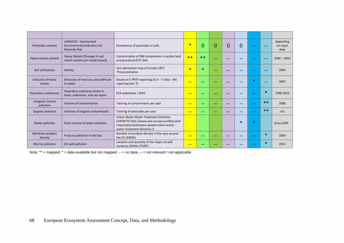
68 European Ecosystem Assessment Concept, Data, and Methodology
Pesticides content HAIR2010 ‐ Harmonized Environmental Indicators for Pesticide Risk
Exceedance of pesticides in soils * 0 0 0 0 ‐‐ ‐‐ depending on input data
Heavy metals content Heavy Metals (Changes in soil metal content are model based)
Concentration of NM components in arable land and grassland (ETC‐SIA) ** ** ‐‐ ‐‐ ‐‐ ‐‐ ‐‐ 2000 – 2050
Soil salinization Salinity Soil salinization map of Europe (JRC) concentration * * ‐‐ ‐‐ ‐‐ ‐‐ ‐‐ 2009
Emission of heavy metals
Emissions of mercury and cadmium to water
Based on E‐PRTR reporting of 2‐‐‐‐7 data ‐ MS reporting (Art 7) ‐‐ ‐‐ ‐‐ ‐‐ ‐‐ * ‐‐ 2007
Hazardous substances Hazardous substance levels in biota, sediments, and sea water
EEA waterbase / WFD ‐‐ ‐‐ ‐‐ ‐‐ ‐‐ ‐‐ * 1998‐2010
Inorganic marine pollution
Volume of contamination Total kg of contaminants per year ‐‐ ‐‐ ‐‐ ‐‐ ‐‐ ‐‐ ** 2006
Organic pollution Volumes of organic contaminants Total kg of pesticides per year ‐‐ ‐‐ ‐‐ ‐‐ ‐‐ ‐‐ ** n/a
Water pollution Point sources of water pollution
Urban Waste Water Treatment Directive (UWWTD) http://www.eea.europa.eu/data‐and‐maps/data/waterbase‐uwwtd‐urban‐waste‐water‐treatment‐directive‐3
* * Since 2009
Maritime accident density
Proxy to pollution in the Sea Number of accident density in the seas around the EU (EMSA) ‐‐ ‐‐ ‐‐ ‐‐ ‐‐ ‐‐ * 2009
Marine pollution Oil spill pollution Location and quantity of the major oil spill incidents (EMSA /ITOPF) ‐‐ ‐‐ ‐‐ ‐‐ ‐‐ ‐‐ * 2012
Note: ** = mapped; * = data available but not mapped; -- = no data; -- = not relevant / not applicable

European Ecosystem Assessment Concept, Data, and Methodology 69
Annex 3 Datasets and indicators available to assess the condition of Pan-European ecosystems
Table 3 Main datasets and indicators to be used in the assessment of ecosystems condition and trends
Condition and trends
Ecosystem Indicator Datasets/ indicator Crop‐land
Grass‐land
Wood‐land and forest
Heath‐land and shrub
Wet‐lands
Rivers and lakes
Marine
Reference year
general Habitat Directive Article 17 Population category and trend (species)Coverage category and trends (habitats) * * ** * * * * 2000‐2012
general Birds Directive Article 12 Status of conservation of wild bird species naturally occurring in the Union * * * * * * * 2012
general Natura 2000 Status of conservation of natural habitats and wild fauna and flora ** ** ** ** ** ‐‐ * 2000‐2012
general IUCN European species assessment
Status of conservation and trends of plants and animal species in Europe * ‐‐ ‐‐ ‐‐ ‐‐ ‐‐ ‐‐ Several
years
Surface Ecosystem size Pan‐European ecosystem map (EEA, ETC‐SIA) ** ** ** ** ** * ‐‐ 2006, 2012
Ecological quality status/surface (ha)
Ecosystem quality (if data only available at level of ecosystem type)
Pan‐European ecosystem condition map (EEA, ETC‐SIA) * * * * * * * 2006
Agro‐ecosystems CAP – Good Agricultural Ecological condition (GAEC)
Minimum soil cover, appropriate machinery use, use of adequate rotation crops, level of protection of permanent pasture, level of water protection against pollution, level of unwanted vegetation in agricultural land
* * ‐‐ ‐‐ ‐‐ ‐‐ ‐‐ n/a
Woodland and forest ecosystems
Forest biomass
Forest quality,Forest growing stock (Gallaun, et al., 2‐‐1‐‐) ‐‐ ‐‐ * ‐‐ ‐‐ ‐‐ ‐‐ 2009
FW, transitional, and coastal waters
WFD –Ecological status % classified less than GES surface water bodies in Europe ‐‐ ‐‐ ‐‐ ‐‐ ‐‐ ** * 2000‐2012
Woodland and forest ecosystems
Naturalness of forests
HNV forest area Biogeographical regions, Tree species maps (EFI) Forest type suitability map (JRC)
‐‐ ‐‐ ** ‐‐ ‐‐ ‐‐ ‐‐ 2009
FW, transitional, and coastal waters
WFD ‐ Nitrogen and phosphorous concentrations in rivers
WaterbaseWFD: mean annual nitrates in rivers reported by MS SEBI‐‐9 indicator on critical load exceedance for nitrogen
‐‐ ‐‐ ‐‐ ‐‐ * ** ‐‐ 2000‐2012

70 European Ecosystem Assessment Concept, Data, and Methodology
FW, transitional, and coastal waters
WFD ‐ Chemical status % of water bodies not achieving good chemical status in transitional and coastal waters (WISE‐WFD) ‐‐ ‐‐ ‐‐ ‐‐ * ** * 2000‐2012
FW, transitional, and coastal waters
WFD ‐ Nitrate concentrations in groundwater
WFD ‐‐ ‐‐ ‐‐ ‐‐ ‐‐ * ‐‐ 2000‐2012
FW, transitional, and coastal waters
WFD ‐ Phosphorous concentrations in lakes
WFD: annual mean phosphorus and nitrate concentration in water bodies ‐‐ ‐‐ ‐‐ ‐‐ ‐‐ * ‐‐ 2000‐2012
FW, transitional, and coastal waters
WFD ‐ Nitrate and phosphate concentrations in coastal water
WFD: trends for nitrogen and phosphorus concentrations in open marine, coastal and transitional waters MSFD: The MSFD pressure analysis will define how widely the land‐based pressures namely nutrient loading from rivers and atmospheric deposition of nitrogen are impacting the marine environment.
‐‐ ‐‐ ‐‐ ‐‐ ‐‐ ‐‐ * 2000‐2012
FW, lakes, transitional, and coastal waters
WFD ‐ % of natural, heavily modified, artificial and unknown status for river, lake, transitional and coastal water bodies
% of classified heavily modified and artificial bodies ‐‐ ‐‐ ‐‐ ‐‐ ‐‐ * ‐‐ 2000‐2012
Coastal and marine Bathing water quality ‐ Bathing water Directive
Water quality during bathing season reported by MS ‐‐ ‐‐ ‐‐ ‐‐ ‐‐ ‐‐ ** 1990‐2014
Marine ecosystems MSFD ‐ Biological diversity quality and occurrence of habitats abundance of species low levels of non‐indigenous species
‐‐ ‐‐ ‐‐ ‐‐ ‐‐ ‐‐ ** 2012
Marine ecosystems Flagship species abundance (EMODNET biology)
species density per ecoregion ‐‐ ‐‐ ‐‐ ‐‐ ‐‐ ‐‐ * 2002‐2011
Marine ecosystems Diffuse attenuation coefficients (JRC‐EMIS)
transparency of the water column ‐‐ ‐‐ ‐‐ ‐‐ ‐‐ ‐‐ * 2002 ‐ 2012
Marine ecosystems chlorophyll concentration (JRC‐EMIS)
Annual average chlorophyll concentration based on satellite observations (EOS MODIS‐A (NASA GSFC)) ‐‐ ‐‐ ‐‐ ‐‐ ‐‐ ‐‐ * 2002 ‐ 2012
Note: ** = mapped; * = data available but not mapped; -- = no data; -- = not relevant / not applicable