European Commission Directorate General Economic and Financial Affairs Using BCS data for tracking...

European CommissionDirectorate General Economic and Financial Affairs

Using BCS data for tracking q-o-q GDP growth

Andreas ReuterBusiness and consumer surveys and

short-term forecast (ECFIN A4.2)

2

Outline

2. Relative weaknesses of the Economic Sentiment Indicator (ESI)

4. Improving the ESI's tracking performance of q-o-q GDP growth

step a: re-constructing the ESI based on "best-performing" survey questions

step b: an ESI with amplified changes

3. Refresher on ESI Construction Method

1. Introduction: the Economic Sentiment Indicator (ESI)

3

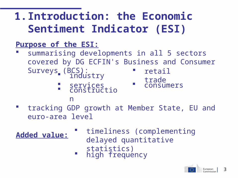
1. Introduction: the Economic Sentiment Indicator (ESI)

Added value: timeliness (complementing delayed quantitative statistics)

high frequency

Purpose of the ESI: summarising developments in all 5 sectors covered by DG

ECFIN's Business and Consumer Surveys (BCS):

services

tracking GDP growth at Member State, EU and euro-area level

industry

construction

retail trade consumers

4

ESI is excellent in tracking GDP growth y-o-y…

2. Relative Weaknesses of the Economic Sentiment Indicator (ESI)

03/1

996

03/1

997

03/1

998

03/1

999

03/2

000

03/2

001

03/2

002

03/2

003

03/2

004

03/2

005

03/2

006

03/2

007

03/2

008

03/2

009

03/2

010

03/2

011

03/2

012

70.00

75.00

80.00

85.00

90.00

95.00

100.00

105.00

110.00

115.00

120.00

-6.00

-4.00

-2.00

0.00

2.00

4.00

6.00

ESI (quarterly levels)GDP growth (quarterly, y-o-y, euro area, rhs)

0.92

0.87

0.68

Correlations:

coincident

leading 1

leading 2

However…

5

ESI is less convincing in tracking GDP growth q-o-q…

2. Relative Weaknesses of the Economic Sentiment Indicator (ESI)

06/1

995

06/1

997

06/1

999

06/2

001

06/2

003

06/2

005

06/2

007

06/2

009

06/2

011

70

80

90

100

110

120

-3

-2

-1

0

1

2

ESI (quarterly levels)

GDP growth (quarterly, q-o-q, euro area, rhs)

06/1

995

06/1

997

06/1

999

06/2

001

06/2

003

06/2

005

06/2

007

06/2

009

06/2

011

30

35

40

45

50

55

60

65

-3

-2

-1

0

1

2

PMI (quarterly levels)


06/1

995

06/1

997

06/1

999

06/2

001

06/2

003

06/2

005

06/2

007

06/2

009

06/2

011

96

97

98

99

100

101

102

103

-3

-2.5

-2

-1.5

-1

-0.5

0

0.5

1

1.5

2

OECD Composite Leading Indicator (quarterly levels)


PMI

0.71 0.87 0.67

0.46 0.65 0.38

0.19 0.37 0.05

Correlations:

coincident

leading 1

leading 2

ESI OECD CLI

2 quarters delay

downturn signalled with:

1 quarter delay

quickness of recovery underestimated

6

ingredients: balance series of 15 survey questions

Effect: values >100 indicate above-average

economic sentiment

3. Refresher on ESI Construction Method

The questions are: seasonally adjusted standardised

allocating weights per sector: Industry: 40% ; Services: 30% ; Consumers: 20% ; Construction: 5% ; Retail Trade: 5%

calculation of arithmetic mean of weighted balances

standardisation of the ESI and: addition of 100 multiplication by 10

Effect: comparability of balance series in

terms of mean and volatility no series dominates development of

ESI due to a higher amplitude

individual indu question has weight of 13,3% (=40% weight / 3 questions)

2/3 of observations will be in the interval [90 ; 110]

(assuming normality)

% of positive answers minus % of negative answers

7


step a: re-constructing the ESI based on "best-performing" survey questions

1. Correlation of all individual survey questions with i) reference series, ii) q-o-q GDP growth:

quarterly averages of balance series

for industry:Gross Value Added in Manufacturingfor services:Gross Value Added in Servicesfor consumers:Household and NPISH final consumption expenditurefor construction:Gross Value Added in Construction

for retail trade:Household and NPISH final consumption expenditure

8

2. Construction of 3 new sector-specific Confidence Indicators (CIs):

CIs summarise overall perceptions / expectations at individual sector level

4. Improving the ESI's tracking performance of q-o-q GDP growth – step a: reconstructing the ESI based on "best-performing" survey questions

calculation: arithmetic mean of (seasonally adjusted) balances for specific questions

questions included in sectoral CIs are also the ones used to construct the ESI

1. CI based on the 2 best performing questions (reg. correlation with reference series & GDP q-o-q)

2. CI based on the 3 best performing questions (reg. correlation with reference series & GDP q-o-q)

3. CI based on all forward-looking questions of the respective sector

3. For each sector: selection of the best CI (reg. correlation with reference series & GDP q-o-q)

9

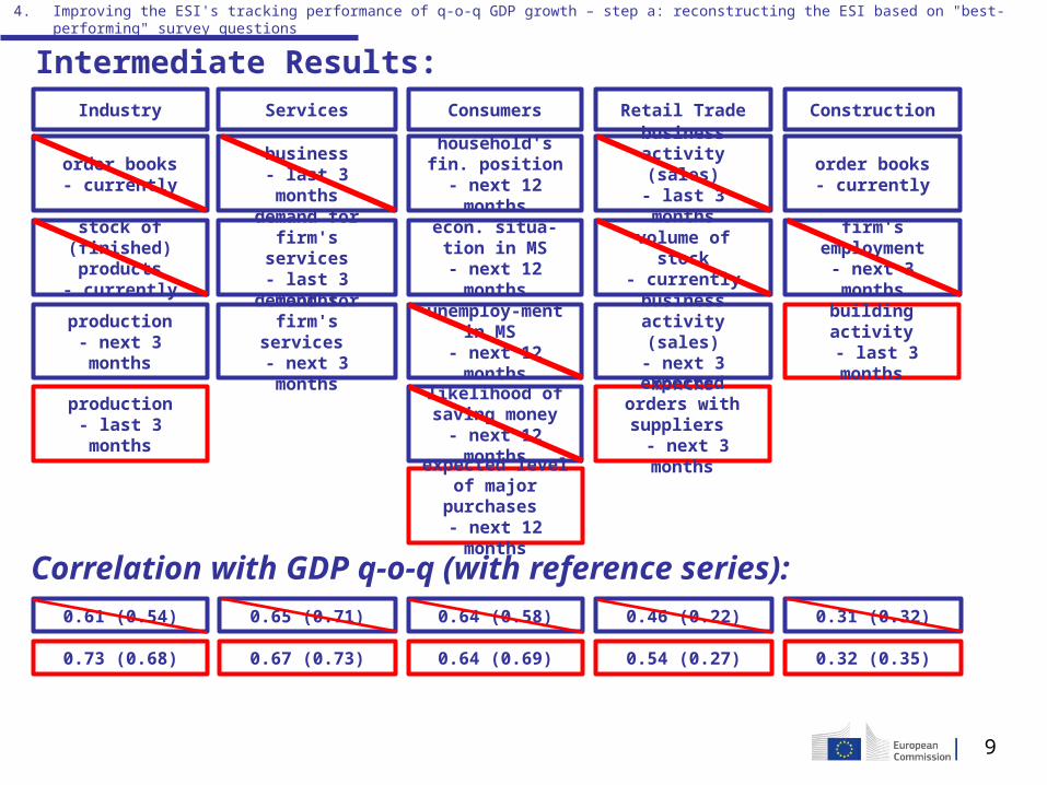
Intermediate Results:


Industry Services Retail TradeConsumers

order books- currently

business- last 3 months

business activity (sales)

- last 3 months

household's fin. position

- next 12 months

stock of (finished) products

- currently

demand for firm's services

- last 3 months

volume of stock- currently

econ. situa-tion in MS

- next 12 months

production- next 3 months

demand for firm's services

- next 3 months

business activity (sales)

- next 3 months

unemploy-ment in MS

- next 12 months

likelihood of saving money

- next 12 months

Construction

order books- currently

firm's employment- next 3 months

production- last 3 months

expected level of major purchases - next 12 months

expected orders with suppliers

- next 3 months

building activity - last 3 months

0.61 (0.54) 0.65 (0.71) 0.46 (0.22)0.64 (0.58)

0.73 (0.68) 0.67 (0.73) 0.54 (0.27)0.64 (0.69)

0.31 (0.32)

0.32 (0.35)

Correlation with GDP q-o-q (with reference series):

10

4. Re-construction of the ESI, using the set of questions of the new CIs:


Slight improvements…

03/1

996

12/1

996

09/1

997

06/1

998

03/1

999

12/1

999

09/2

000

06/2

001

03/2

002

12/2

002

09/2

003

06/2

004

03/2

005

12/2

005

09/2

006

06/2

007

03/2

008

12/2

008

09/2

009

06/2

010

03/2

011

12/2

011

09/2

012

60

70

80

90

100

110

120

-03

-02

-01

00

01

ESI with new questions (quarterly levels)ESI (quarterly levels)GDP growth (quarterly, q-o-q, euro area, rhs)

Turning points:modified ESI records 0-change in quarter where GDP-downturn starts, while the ESI still signals a rise

Amplitude:modified ESI records steeper downward slope than ESI, being more in line with GDP-growth

modified ESI

0.71 0.77 8 %

0.46 0.51 12%

0.19 0.25 30%

Correlations:

coincident

leading 1

leading 2

ESI improvement

11

step b: an ESI with amplified changes

Intuition of the approach:


Comparable changes in the ESI should be taken more "seriously", when reflected by many survey questions.

Example:

Indu

stry

Q1

Indu

stry

Q5

Servic

es Q

2

Servic

es Q

3

Consu

mpt

ion Q

2

Consu

mpt

ion Q

4

Consu

mpt

ion Q

9

Retail

Q3

Retail

Q4

Const

ruct

ion Q

1

Const

ruct

ion Q

3

-2

-1.5

-1

-0.5

0

0.5

change in 1999Q1 (compared to previous quarter)change in 2000Q4 (compared to previous quarter)

Change in modified ESI: -1.8

Change in modified ESI: -2

Instead:change in ESI should be-2*x (with x > 1)

standard deviation of balance series

>>>> change in ESI should be multiplied, if a critical amount of questions changes in the same direction

We propose: 8 (out of 11) questions We propose: multiplication by 3

12

Calculation of the new method:

4. Improving the ESI's tracking performance of q-o-q GDP growth – step b: an ESI with amplified growth

1. Sum all standardised weighted questions per quarter:

2. Calculate the (modified) ESI:

Variable is called: ZNEW

sum of weighted standardised questions (per quarter)

13


3. Calculate the absolute change of ZNEW per quarter:

4. Calculate for each quarter a variable taking value 1 if >=8 questions go up / go down :

Variable is called: ZNEW change

(trigger variable)

Variable is called: ZNEW change (amplified)

5. Re-calculate "ZNEW change" mutiplying it by 3 (only in case the "trigger variable" has value 1):

sum of weighted standardised questions (per quarter)

14


6. Re-calculate ZNEW, adding "ZNEW change (amplified)" of quarter t to "ZNEW" of quarter t-1:

Variable is called: ESINEW (amplified change)

Variable is called:

ZNEW (amplified)

7. Standardise "ZNEW (amplified)" and thus obtain a new ESI with amplified change:

15


Results:

03/1

996

03/1

997

03/1

998

03/1

999

03/2

000

03/2

001

03/2

002

03/2

003

03/2

004

03/2

005

03/2

006

03/2

007

03/2

008

03/2

009

03/2

010

03/2

011

03/2

012

60

70

80

90

100

110

120

-3

-2.5

-2

-1.5

-1

-0.5

0

0.5

1

1.5

current ESI (quarterly levels)

ESINEW - amplified change (quarterly levels)

PMI (quarterly levels, rescaled to long-term mean of 100)


improvements:

compared to current ESI:

compared to PMI:

"micro"-volatility of GDP better captured

2008-downturn announced by steeper slope (more in line with GDP)

2009-upswing reflected with steeper slope (in line with GDP)

"micro"-volatility of GDP better captured

better leading properties

time-period current ESI PMIESINEW (ampl.)

increase compared to current ESI

increase compared to

PMI

98Q3 – 02Q1 0.58 (0.28) 0.74 (0.54)0.76 (0.52) 31% (85%) 4% (-4%)

02Q2 – 07Q1 0.79 (0.64) 0.86 (0.63)0.85 (0.69) 8% (8%) -1% (10%)

07Q2 – 12Q2 0.74 (0.39) 0.89 (0.61)0.91 (0.73) 23% (87%) 2% (18%)

98Q3 – 07Q1 0.64 (0.41) 0.79 (0.58)0.79 (0.58) 25% (41%)

98Q3 – 12Q2 0.75 (0.49) 0.87 (0.65)0.90 (0.73) 20% (51%)

0% (0%)

3% (12%)

Correlation with GDP growth q-o-q (in brackets: leading 1 correlations)

16

Conclusion: BCS data can be used to construct indicator tracking q-o-q

GDP growth satisfactorily

key of the approach: consider not only the (average) values of the balance series, but also the amount of series moving up/down

approach is still in its infancy and needs further testing

17


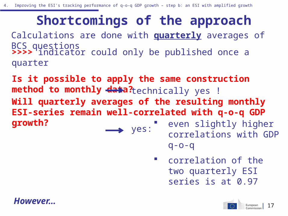
Shortcomings of the approach

Is it possible to apply the same construction method to monthly data?

Calculations are done with quarterly averages of BCS questions

>>>> indicator could only be published once a quarter

technically yes !

Will quarterly averages of the resulting monthly ESI-series remain well-correlated with q-o-q GDP growth?

yes: even slightly higher correlations with GDP q-o-q

correlation of the two quarterly ESI series is at 0.97

However…

18

4. Improving the ESI's tracking performance of q-o-q GDP growth – step b: an ESI with amplified growth – Shortcomings of the approach

Problem of constructing ESI with amplified changes for monthly data:

too high volatility

1/1/

1996

1/1/

1997

1/1/

1998

1/1/

1999

1/1/

2000

1/1/

2001

1/1/

2002

1/1/

2003

1/1/

2004

1/1/

2005

1/1/

2006

1/1/

2007

1/1/

2008

1/1/

2009

1/1/

2010

1/1/

2011

1/1/

2012

55

65

75

85

95

105

115

125

ESINEW - amplified changes (monthly levels) current ESI (monthly levels)

Sep 2009: in upswing-period, ESINEW with amplified changes drops by 10 points (=1 standard deviation)

19


If amplification is applied in t-1, but not in t, ESI will usually suggest a drop in sentiment in t (also in case the underlying data continues the upward/downward trend of t-1)

Source of volatility (note: amplifying changes does not only increase the amplitude of the series, but also its volatility):

Jan Feb Mar Apr94

96

98

100

102

104

106

unamplified ESIESI (amplified change): assuming 8 questions go up in Feb

+2 +2 +2

+2*3 = +6

This additional volatility improves the fit of our quarterly series, but renders the monthly series TOO volatile.

Main reason for this difference: criterion for amplification is more restrictive in case of quarterly set-up:

for quarterly: >= 8 questions must have gone up/down over 3 months-period (amplification in 63% of quarters)

for monthly: >= 8 questions must have gone up just one month (amplification in 73% of the months)

20


Solution: When multiplying change of t (compared to t-1), the

resulting amplified change should be added to ESI for month t, but also ESI of t+1 and t+2 (1/3 of the change respectively should be added).

Approach smoothens the monthly curve substantially…

4/1/

1996

4/1/

1997

4/1/

1998

4/1/

1999

4/1/

2000

4/1/

2001

4/1/

2002

4/1/

2003

4/1/

2004

4/1/

2005

4/1/

2006

4/1/

2007

4/1/

2008

4/1/

2009

4/1/

2010

4/1/

2011

4/1/

2012

55

65

75

85

95

105

115

125

ESINEW - amplified changes (monthly levels)ESINEW - amplified changes distributed over 3 months (monthly levels)

When constructing quarterly averages, correlations with q-o-q GDP growth remain high.

European Commission Directorate General Economic and Financial Affairs Using BCS data for tracking...

Documents

Transcript of European Commission Directorate General Economic and Financial Affairs Using BCS data for tracking...