EuroGOOS Arctic Task Team Planning Document Draftcryos.ssec.wisc.edu/docs/EuroGOOS_ATT_plan.pdf ·...
45
EuroGOOS Arctic Task Team Planning Document Draft Edited by S. Sandven, E. Fahrbach, E. Buch, O. M. Johannessen, H. Cattle, L. Toudal and T. Vihma November 2004
Transcript of EuroGOOS Arctic Task Team Planning Document Draftcryos.ssec.wisc.edu/docs/EuroGOOS_ATT_plan.pdf ·...

EuroGOOS Arctic Task Team
Planning Document
DraftEdited by S. Sandven, E. Fahrbach, E. Buch, O. M. Johannessen, H. Cattle, L. Toudal and T. Vihma
November 2004


Contents1 Summary . . . . . . . . . . . . . . . . . . . . . . . . . . . . . . . . . . . . . . . . . . . . . . . . . . . . . . . . . . . 11.1 State-of-the-art . . . . . . . . . . . . . . . . . . . . . . . . . . . . . . . . . . . . . . . . . . . . . . . . . . . . . . . . . . . . . . . 11.2 Rationale . . . . . . . . . . . . . . . . . . . . . . . . . . . . . . . . . . . . . . . . . . . . . . . . . . . . . . . . . . . . . . . . . . . 11.3 Objectives . . . . . . . . . . . . . . . . . . . . . . . . . . . . . . . . . . . . . . . . . . . . . . . . . . . . . . . . . . . . . . . . . . 51.4 Users of operational oceanography . . . . . . . . . . . . . . . . . . . . . . . . . . . . . . . . . . . . . . . . . . . . . . . 51.4.1 Operational users who need near real time monitoring and forecasting services . . . . . . . . . . . . 51.4.2 Climate monitoring and modelling . . . . . . . . . . . . . . . . . . . . . . . . . . . . . . . . . . . . . . . . . . . . . . . . 51.4.3 Environmental monitoring and resource management . . . . . . . . . . . . . . . . . . . . . . . . . . . . . . . . 51.5 Links to ongoing programmes and organisations . . . . . . . . . . . . . . . . . . . . . . . . . . . . . . . . . . . . 51.6 Implementation Process . . . . . . . . . . . . . . . . . . . . . . . . . . . . . . . . . . . . . . . . . . . . . . . . . . . . . . . 6
2 Natural Conditions . . . . . . . . . . . . . . . . . . . . . . . . . . . . . . . . . . . . . . . . . . . . . . . . . . . 92.1 Ice-covered and ice-free areas . . . . . . . . . . . . . . . . . . . . . . . . . . . . . . . . . . . . . . . . . . . . . . . . . . 92.2 Description of the Arctic Ocean and the adjacent seas . . . . . . . . . . . . . . . . . . . . . . . . . . . . . . . 10
3 Variables and Observing Strategies . . . . . . . . . . . . . . . . . . . . . . . . . . . . . . . . . . . . 133.1 Sea ice . . . . . . . . . . . . . . . . . . . . . . . . . . . . . . . . . . . . . . . . . . . . . . . . . . . . . . . . . . . . . . . . . . . . 133.1.1 Ice concentration/extent and navigational ice charts . . . . . . . . . . . . . . . . . . . . . . . . . . . . . . . . . 143.1.2 Ice thickness . . . . . . . . . . . . . . . . . . . . . . . . . . . . . . . . . . . . . . . . . . . . . . . . . . . . . . . . . . . . . . . 173.1.3 Ice drift . . . . . . . . . . . . . . . . . . . . . . . . . . . . . . . . . . . . . . . . . . . . . . . . . . . . . . . . . . . . . . . . . . . . 183.1.4 Icebergs . . . . . . . . . . . . . . . . . . . . . . . . . . . . . . . . . . . . . . . . . . . . . . . . . . . . . . . . . . . . . . . . . . . 203.2 Temperature, salinity and currents . . . . . . . . . . . . . . . . . . . . . . . . . . . . . . . . . . . . . . . . . . . . . . 203.2.1 Satellite observations of sea surface temperature and ocean colour . . . . . . . . . . . . . . . . . . . . 203.2.2 Ship observations . . . . . . . . . . . . . . . . . . . . . . . . . . . . . . . . . . . . . . . . . . . . . . . . . . . . . . . . . . . 203.2.3 Measurements from moored systems . . . . . . . . . . . . . . . . . . . . . . . . . . . . . . . . . . . . . . . . . . . . 223.2.4 Measurements from free drifting or propelled autonomous systems . . . . . . . . . . . . . . . . . . . . . 233.2.5 Planned systems for under-ice monitoring . . . . . . . . . . . . . . . . . . . . . . . . . . . . . . . . . . . . . . . . . 243.3 Sea level, surface topography and wave forecasting . . . . . . . . . . . . . . . . . . . . . . . . . . . . . . . . 253.3.1 Tide gauge measurements . . . . . . . . . . . . . . . . . . . . . . . . . . . . . . . . . . . . . . . . . . . . . . . . . . . . 253.3.2 Sea surface topography from altimetry . . . . . . . . . . . . . . . . . . . . . . . . . . . . . . . . . . . . . . . . . . . 253.3.3 Wave forecasting . . . . . . . . . . . . . . . . . . . . . . . . . . . . . . . . . . . . . . . . . . . . . . . . . . . . . . . . . . . . 263.4 Boundary conditions . . . . . . . . . . . . . . . . . . . . . . . . . . . . . . . . . . . . . . . . . . . . . . . . . . . . . . . . . 263.4.1 Meteorology . . . . . . . . . . . . . . . . . . . . . . . . . . . . . . . . . . . . . . . . . . . . . . . . . . . . . . . . . . . . . . . . 263.4.2 River runoff . . . . . . . . . . . . . . . . . . . . . . . . . . . . . . . . . . . . . . . . . . . . . . . . . . . . . . . . . . . . . . . . 273.5 Tracers . . . . . . . . . . . . . . . . . . . . . . . . . . . . . . . . . . . . . . . . . . . . . . . . . . . . . . . . . . . . . . . . . . . . 283.6 Oil spills and other pollutants . . . . . . . . . . . . . . . . . . . . . . . . . . . . . . . . . . . . . . . . . . . . . . . . . . . 29
4 Modelling and Forecasting . . . . . . . . . . . . . . . . . . . . . . . . . . . . . . . . . . . . . . . . . . . 314.1 Example of climate models: The Bergen climate model . . . . . . . . . . . . . . . . . . . . . . . . . . . . . . 314.2 Example of operational forecasting: The TOPAZ system . . . . . . . . . . . . . . . . . . . . . . . . . . . . . 314.3 Ocean Forecasting by the MI–POM model system . . . . . . . . . . . . . . . . . . . . . . . . . . . . . . . . . . 324.4 Example of a regional model: the Barents Sea model . . . . . . . . . . . . . . . . . . . . . . . . . . . . . . . . 33
5 Data Exchange . . . . . . . . . . . . . . . . . . . . . . . . . . . . . . . . . . . . . . . . . . . . . . . . . . . . . 356 Dissemination . . . . . . . . . . . . . . . . . . . . . . . . . . . . . . . . . . . . . . . . . . . . . . . . . . . . . . 377 References . . . . . . . . . . . . . . . . . . . . . . . . . . . . . . . . . . . . . . . . . . . . . . . . . . . . . . . . 398 Contributors . . . . . . . . . . . . . . . . . . . . . . . . . . . . . . . . . . . . . . . . . . . . . . . . . . . . . . . 459 Appendix . . . . . . . . . . . . . . . . . . . . . . . . . . . . . . . . . . . . . . . . . . . . . . . . . . . . . . . . . . 47


Arctic Task Team Plan 1
1.1 State-of-the-artThe Arctic climate of the 20th century hasundergone major fluctuations which are charac-terised by a significant warming in the last twodecades. The main features of these fluctuations area substantial warming between 1925 and 1945, amarked cooling in 1950–1970 and finally anongoing warming trend which started around 1980(Johannessen et al., 2003). These events have notbeen restricted to the Arctic, but the strength of thewarming has by far been most pronounced in theArctic region, as the climate models predict. Thewarming predicted for the high Arctic is 3–4 °C inwinter during the next 50 years, more than twicethe global average, while the ice cover is predictedto reduce by ~40% during summer and ~10%during winter according to ECHAM41 andHadCM32 simulations (Johannessen et al., 2004a).This suggests that the Arctic may be the location ofthe most rapid and dramatic climate changes duringthe 21st century, with major ramifications for mid-latitude climate. Examples of model predictions ofair temperature and sea ice extent are shown inFigure 1.The Arctic region has over the last 2–3 decadeswarmed more than other regions of the world, andin the same period the sea ice cover has decreasedby ~10% (Johannessen et al., 1999; 2004a) whereasthe ice thickness has decreased up to 40%(Rothrock et al., 1999). Other observed changesinclude a warming of the Atlantic water in theArctic Ocean (Morison et al., 1998), increasedprecipitation in the Arctic regions and higher riverdischarge into the Arctic ocean (Peterson et al.,2002). During the last decades detected changesinclude a significant freshening of the deep NorthAtlantic Ocean (Dickson et al., 2002), warming inthe deep water of the Nordic Seas (Østerhus andGammelsrød, 1999) and a decrease in deepoverflow in the Faeroe Bank Channel (Hansen etal., 2001). The oceanic fluxes of heat and fresh-water between the North Atlantic, Nordic Seas andArctic Ocean are a key component of the high-latitude climate system (Oliver and Heywood,2003).
The Arctic Ocean plays a major role concerning thesurface energy and freshwater budgets, because it isa large and effective heat sink, and it exports asignificant amount of freshwater into the NorthAtlantic, into areas of deep water formation like theGreenland, Irminger and Labrador Seas, fromwhere the global oceanic thermohaline circulationis driven. Improved monitoring systems are neededto provide consistent and long-term data on the ice-ocean circulation in the Arctic Ocean including theFram Strait and Nordic Seas. Monitoring systemsshould have a central role in detection and verifi-cation of climate variability and trends. Monitoringand forecasting of the environmental conditions isalso needed to support all types of marine opera-tions to secure sustainable and safe development inhigh latitudes.
1.2 RationaleThe recent Arctic Climate Impact Assessmentstudies (ACIA, 2004) have identified a number ofsevere impacts of Arctic warming on society.Changes in air temperature, precipitation, riverdischarge, sea ice, permafrost, glaciers and sealevel have been documented and further changesare expected over the next decades. The Arcticregion is coming under increasing pressure fromunsustainable development with pollution and othernegative effects on the environment. The exploi-tation of resources, including sea transportation andoffshore operations will be heavily affected by theclimate variability and long-term changes at highlatitudes. The northeast Atlantic, includingGreenland and Icelandic waters, the Barents Seaand other Arctic ice edge regions provide 20% ofthe world’s fish catch. Ocean temperature is one ofthe key variables that influence fisheries. Forexample, the temperature changes observed in theKola section since the early 1900s show strongcorrelation with variability in spawning stockbiomass of Norwegian spring-spawning herring(Thorsen and Østvedt, 2000), as shown in Figure 2.Monitoring the ocean environment is an importantelement in the management of fishery resources. Tanker transportation of oil and gas in the NorthernSea Route between Russia and Western Europe isincreasing, with associated risks for accidents anddamage to the environment. The amounts of oil
1 Summary
1. ECHAM4: Max Planck Institute for Meteorology’s climate model (http://www.dkrz.de)
2. HadCM3: The Hadley Centre climate model http://www.metoffice.co.uk

Summary2
transportation along the Norwegian coastline fromNorthwest Russia has increased considerablyduring recent years (Frantzen and Bambuliak,
2003), causing severe concerns that accidents likethe Exxon Valdez in 1989 and the Prestige in 2002can happen in European Arctic seas. Long-term
Figure 1 Climate prediction scenario on doubling of CO2 using the Bergen Climate Model (www.bcm.uib.no). Temper-ature change for the Arctic and sub-Arctic areas is shown for summer (a) and winter (b). Prediction of sea ice extent in
2070 is shown for September (c) and March (d) where the red area is the control run and the white area is the CO2 doubling.
a) b)
c) d)
Figure 2 (a) The red line shows fluctuations of spawning stock biomass (SSB) of Norwegian spring-spawning herring (unit: recruits 0-grp) and the blue line shows mean annual temperature in °C at the Kola section, (b) Distribution area of Norwegian spring-spawning herring in the north-east Atlantic region. Open arrows: migration route of herring during summer; thick arrows: main flow of Atlantic water; thin arrows: main flow of cold Arctic water
(Thoresen and Østvedt, 2000).
a) b)

Arctic Task Team Plan 3
effects on the wildlife from the Exxon Valdezaccident have recently been documented, showingunexpected persistence of toxic subsurface oil withchronic exposure to the Alaskan coastal ecosystem(Peterson et al., 2003). Various offshore operationsin ice-covered waters will increase such as drilling,production, pipeline deployment in the seabed, andbuilding of terminals in several locations along theArctic coasts. All these activities will increase therisk of accidents and severe pollution of the fragileArctic environment. The oil and gas resources inArctic regions are huge and increased exploitationof these resources is expected in the future, withcorresponding increase in tanker traffic andoffshore operations. Northwest Russia and theBarents Sea has 25% of the world’s unexploitedpetroleum resources (Figure 3), which will have animpact on global energy and transport policies. Research expeditions and tourist traffic in Arcticwaters are increasing. After the first icebreakerexpedition to the North Pole with the Russianicebreaker Arctica in 1977, more than 50 vesselshave visited the Pole during the summer periods.Over the last 10 years there have been severalvessels to the Pole every year, most of them touristexpeditions.Transit transportation between Europe and the EastAsia and the west coast of North America throughthe Northern Sea Route can become economicallyattractive in the perspective of reduced sea icecover. Transit expeditions with non-Russianvessels during summer started in 1991 with theL’Astrolabe voyage. Several demonstrationvoyages have taken place during the 1990s, andcommercial transit traffic is expected to develop ina longer perspective (Johannessen et al., 2000). The Arctic areas have rough weather and ice condi-tions which require improvement of operationalmonitoring and forecasting services in order tosafeguard all types of marine and coastal opera-tions. The operational services should also includelong-term data archiving services to build upstatistics of the environmental conditions. TheInternational Maritime Organisation (IMO)develops the regulations and standards for legis-lation in countries with maritime activities. Guide-lines for ships operating in Arctic ice-coveredwaters have recently been issued (IMO, 2002),specifying requirements for ship construction,machinery, equipment, crews, training and opera-tional procedures. Furthermore, the guidelines haverules for environmental protection and damagecontrol.
The Arctic Council is a key inter-governmentalbody focusing on protection of the Arcticenvironment and sustainable development as ameans of improving economic, social and culturalwell-being. The Arctic Council provides amechanism to address the common concerns andchallenges faced by the Arctic governments and thepeople of the Arctic. The Arctic Council runsseveral programmes, which need monitoring anddata for assessment of the environment of theArctic areas. One working group is PAME:Protection of the Arctic Marine Environment withresponsibilities to take preventative and othermeasures, directly or through competent interna-tional organisations, regarding marine pollution inthe Arctic, irrespective of origin. PAME hasrecently produced the Snap Shot Analysis ofMaritime Activities in the Arctic (PAME, 2000)and Guidelines for Arctic Oil and Gas (PAME,2002) activities to minimise negative impacts onthe environment (Figure 4). The other workinggroups include AMAP (Arctic Monitoring andAssessment Programme), CAFF (Conservation ofArctic Flora and Fauna), EPPR (EmergencyPrevention, Preparedness and Response) andSDWG (Sustainable Development).The Commission on Oceanography and MarineMeteorology under WMO/IOC has issued a reporton the need to establish improved observingsystems for the polar regions (JCOMM, 2000). TheGlobal Climate Observing System underWMO/IOC has produced an implementation planin support of the United Nations FrameworkConvention on Global Change (GCOS, 2004)where global ocean and sea ice observations are onthe list of essential climate variables. The European Commission and the EuropeanSpace Agency have jointly initiated GMES: GlobalMonitoring for Environment and Security, wherethe overall objective is to build up Europeancapacity to provide operational monitoring servicesusing spaceborne data as a key component (CEC,2004). Services developed under GMES shallenable decision-makers in Europe to acquire thecapacity for global as well as regional monitoringso as to effectively realise the EU’s objectives in awide variety of policy areas. Monitoring the Arcticis one of the thematic areas of the GMES services.Operational services on met-ice-ocean conditionsin the Arctic Ocean and the Nordic Seas areextremely important for safe and cost-effectiveindustrial and transport activities as well as forprotection of the vulnerable environment. In orderto improve the operational services, it is necessary

Summary4
to develop forecasting systems using numericalmodels and data assimilation techniques.Furthermore, availability of marine observationsand development of information disseminationservices are essential for improvement of services.The marine observations that form the basis for
operational services are basically the same as thoseneeded for climate research. It is therefore relevantthat these two topics are considered simultaneouslywhen planning an Arctic marine monitoring andforecasting system.
Figure 3 Map of the oil and gas fields in the Barents Sea and Pechora Sea. (Barlindhaug, 2004).
Figure 4 Concrete Island Drilling Structure (CIDS) in the Beaufort Sea, Alaska (PAME, 2002)
Arctic Task Team Plan 5
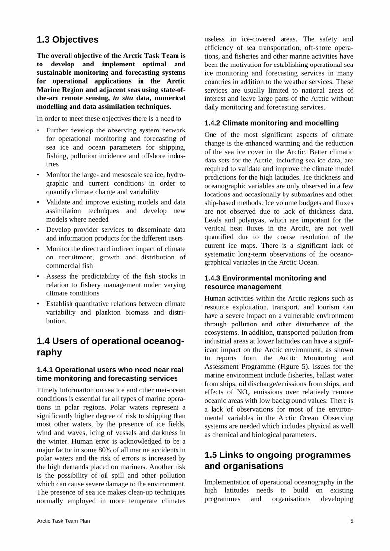
1.3 ObjectivesThe overall objective of the Arctic Task Team isto develop and implement optimal andsustainable monitoring and forecasting systemsfor operational applications in the ArcticMarine Region and adjacent seas using state-of-the-art remote sensing, in situ data, numericalmodelling and data assimilation techniques.In order to meet these objectives there is a need to • Further develop the observing system network
for operational monitoring and forecasting ofsea ice and ocean parameters for shipping,fishing, pollution incidence and offshore indus-tries
• Monitor the large- and mesoscale sea ice, hydro-graphic and current conditions in order toquantify climate change and variability
• Validate and improve existing models and dataassimilation techniques and develop newmodels where needed
• Develop provider services to disseminate dataand information products for the different users
• Monitor the direct and indirect impact of climateon recruitment, growth and distribution ofcommercial fish
• Assess the predictability of the fish stocks inrelation to fishery management under varyingclimate conditions
• Establish quantitative relations between climatevariability and plankton biomass and distri-bution.
1.4 Users of operational oceanog-raphy
1.4.1 Operational users who need near real time monitoring and forecasting servicesTimely information on sea ice and other met-oceanconditions is essential for all types of marine opera-tions in polar regions. Polar waters represent asignificantly higher degree of risk to shipping thanmost other waters, by the presence of ice fields,wind and waves, icing of vessels and darkness inthe winter. Human error is acknowledged to be amajor factor in some 80% of all marine accidents inpolar waters and the risk of errors is increased bythe high demands placed on mariners. Another riskis the possibility of oil spill and other pollutionwhich can cause severe damage to the environment.The presence of sea ice makes clean-up techniquesnormally employed in more temperate climates
useless in ice-covered areas. The safety andefficiency of sea transportation, off-shore opera-tions, and fisheries and other marine activities havebeen the motivation for establishing operational seaice monitoring and forecasting services in manycountries in addition to the weather services. Theseservices are usually limited to national areas ofinterest and leave large parts of the Arctic withoutdaily monitoring and forecasting services.
1.4.2 Climate monitoring and modellingOne of the most significant aspects of climatechange is the enhanced warming and the reductionof the sea ice cover in the Arctic. Better climaticdata sets for the Arctic, including sea ice data, arerequired to validate and improve the climate modelpredictions for the high latitudes. Ice thickness andoceanographic variables are only observed in a fewlocations and occasionally by submarines and othership-based methods. Ice volume budgets and fluxesare not observed due to lack of thickness data.Leads and polynyas, which are important for thevertical heat fluxes in the Arctic, are not wellquantified due to the coarse resolution of thecurrent ice maps. There is a significant lack ofsystematic long-term observations of the oceano-graphical variables in the Arctic Ocean.
1.4.3 Environmental monitoring and resource managementHuman activities within the Arctic regions such asresource exploitation, transport, and tourism canhave a severe impact on a vulnerable environmentthrough pollution and other disturbance of theecosystems. In addition, transported pollution fromindustrial areas at lower latitudes can have a signif-icant impact on the Arctic environment, as shownin reports from the Arctic Monitoring andAssessment Programme (Figure 5). Issues for themarine environment include fisheries, ballast waterfrom ships, oil discharge/emissions from ships, andeffects of NOx emissions over relatively remoteoceanic areas with low background values. There isa lack of observations for most of the environ-mental variables in the Arctic Ocean. Observingsystems are needed which includes physical as wellas chemical and biological parameters.
1.5 Links to ongoing programmes and organisations Implementation of operational oceanography in thehigh latitudes needs to build on existingprogrammes and organisations developing

Summary6
observing and modelling systems for the ArcticOcean and surrounding seas. The organisation ofthe EuroGOOS ATT will follow the functionalstructure of GOOS shown in Figure 6, where‘liaison and integration’ will include links to ArcticCouncil Working Groups, GCOS, JCOMM, CliC,GMES, IABP, various EU-funded projects, andnational monitoring programmes for the Arctic andNordic Seas. Some programmes and projects dealwith topics related to short-term operationalservices, while others deal with climate monitoringand research. GMES is a key programme in Europeto develop satellite monitoring systems, aiming todevelop European operational services in supportof public demand and policy-driven requirements
for information. Several programmes and projectsrelevant for the EuroGOOS ATT are listed in Table1. The implementation of operational oceanographyin the Arctic will build on the observing methodsand modelling systems developed in these projects.Links also need to be established with activities inUSA, Canada, Russia and other countries withinterests in the Arctic.
1.6 Implementation ProcessInitiatives have been taken to create an ArcticGOOS and the planning process has started. Anumber of parallel activities are ongoing which canmake contributions to the development of opera-
Figure 5 Marine pathways of pollutants are illustrated by a) Radionuclides from storage and handling of spent nuclear fuel and waste, operation of nuclear power plants and vessels and military installations in Europe are trans-ported by ocean currents; b) sea ice drift is also a potential mechanism for transport of pollutants over large areas.
Copyright: AMAP
a) b)
Figure 6 The GOOS functional structure

Arctic Task Team Plan 7
tional oceanography in the Arctic and surroundingseas. The Global Climate Observing System hasproduced an Implementation Plan which identifiesa number of actions to be taken to establishobserving systems, many of which are directlyrelated to the polar regions (GCOS, 2004). The GMES programme, initiated jointly by the EUand ESA, aims to develop and establish monitoringservices by 2008. A number of GMES projects arefunded to develop use of satellite Earth Observation(EO) in operational monitoring, including severalArctic projects (see Table 1). GMES is amechanism to fund development and implemen-tation of observing and modelling systems for thehigh latitudes where polar orbiting EO satellites areparticularly useful. The ESA GMES programme has defined severalkey service elements to be implemented against thebackground of user needs and ongoing develop-ments in many applications of satellite data,including sea ice monitoring and other polarthemes. The GMES includes satellite spacesegments and ground segments, data provision anddistribution, service providers, research and devel-opment, and links to user groups who are the recip-ients of the data products. GMES builds linksbetween research institutions and operational insti-tutions and between climate monitoring and opera-tional services (monitoring and forecasting). TheFinal Report form the GMES initial period 2001–2003 outlines a number of actions for the imple-mentation of operational services within the nextfive years (GMES, 2004). The ongoing Arctic/Subarctic Ocean Fluxes(ASOF) programme aims to measure and model thevariability of fluxes between the Arctic Ocean andthe Atlantic Ocean using arrays of current metermoorings in all the key straits as the main observingmethod. The European component of ASOF isfunded for 2002–2005 by the EU Fifth FrameworkProgramme. The International Polar Year (IPY), which isplanned for 2007–2008 under the leadership of theInternational Council for Science, will consist ofinternationally coordinated interdisciplinary scien-tific research and observations focused on theEarth’s polar regions. IPY offers an opportunity todevelop and implement new observing systems forthe Arctic and perform intensive field campaignsand data collection. IPY 2007–2008 will thus
provide a framework and impetus to undertakeprojects that normally could not be achieved by anysingle nation. The IPY Planning Group hasdeveloped a science plan and implementationstrategy (IPY, 2004) available at www.ipy.org.An EU-funded project “Climate of the Arctic andits Role for Europe (CARE)—a Europeancomponent of the International Polar Year” willduring 2005–2006 plan a number of climate-related studies as part of IPY (Johannessen et al.,2004b).The proposed Arctic Ocean Observing System(AOOS) will deploy a number of observingplatforms on ice floes and in the deep water under-neath the sea ice cover. AOOS is part of the ArcticOcean Science Board–CliC observing plan for theIPY (Dickson, 2004). AOOS addresses a number oftechnical challenges that will make a significantcontribution to operational observing systems suchas near real time data transmission from deep oceanplatforms under the sea ice.Monitoring of sea ice will be part of the IntegratedGlobal Observing Strategy Cryosphere Theme(IGOS-Cryo), which was initiated in May 2004when a concept paper was presented to the IGOSPartners (IGOS 2004). The concept paper wasprepared by people from the World ClimateResearch Programme (WCRP) Climate andCryosphere (CliC) project in collaboration with theScientific Committee on Antarctic Research(SCAR), and in consultation with several IGOSpartners. The response was favourable, and theIGOS Partners agreed that the cryosphere is veryimportant for IGOS and encouraged the proposersto proceed. The next major step is to generate atheme report in 2005. The report will review theneeds in observing data and products, analyse thecurrent state and future of these observations, andpropose feasible objectives for the development ofthe observations which represent a consensusbetween most important data users and dataproviders. On the basis of the consensus, the Themeteam proposes a plan of actions and developments.These actions must have clearly specified objec-tives, implementing organisations, deadlines, anindication of resources needed and of readiness bythe data providers to commit the resources. TheIGOS Partners consider the report and decidewhether it can go to the Implementation Phase.

Summary8
Table 1 Programmes and organisations with activities of relevance to the EuroGOOS ATT
Programmes Objective and Homepage
Global Climate Observing System (GCOS) 1992–
Programme under WMO and IOC to ensure that observations and information needed to address climate-related issues are obtained and made available to all potential users. http://www.wmo.ch/web/gcos/gcoshome.html
International Arctic Buoy Programme (IABP), 1979–
Operates a network of ice buoys in the Arctic Ocean to provide meteorological and oceanographic data for real-time monitoring. http://iabp.apl.washington.edu/
Arctic Climate Impact Assessment (ACIA), 2000–
Evaluates and synthesises knowledge on climate variability, climate change, and increased ultraviolet radiation and their consequences. http://www.acia.uaf.edu/
Climate Variability and Predictability (CliVar) 1995–
WCRP programme to study the natural climate variability and anthropogenic climate change. http://www.clivar.org/
Arctic Climate System Study (ACSYS), 1994–2003.
Completed WCRP programme to ascertain the role of the Arctic in global climate. http://acsys.npolar.no/
Climate and Cryosphere (CliC), 2003–
WCRP programme to assess and quantify the impacts of climate variability of all the cryospheric components on both hemispheres. http://clic.npolar.no
A Study of Environmental Arctic Change (SEARCH), 2003–
US programme to study the full scope of the changes going on in the Arctic psc.apl.washington.edu/search/
Arctic Monitoring and Assessment Programme (AMAP), 1991–
Programme under the Arctic Council to provide information on the status of, and threats to, the Arctic environment. http://www.amap.no
Protection of the Arctic Marine Environment (PAME), 1993–
Programme under the Arctic Council to address policy, non-emergency pollution prevention and control measures for protection of the Arctic marine environment http://www.pame.is
Arctic Subarctic Ocean Flux Array for European Climate (ASOF), 2003–2005.
Ongoing programme to measure and model the variability of fluxes between the Arctic Ocean and the Atlantic Ocean. The European component is co-funded by EU. http://asof.npolar.no/index.html
GMES projects under ESA's GSE programme (2003–2008)
ESA Earthwatch GMES Service Element (GSE) is a 5 year programme dedicated to GMES. http://earth.esa.int/gmes/index.html. Sea ice monitoring project: see http://www.icemon.org
Arctic Operational Platform (ARCOP), 2002–2005.
EU-funded project on technological, environmental, economic and legislative aspects of Arctic shipping and oil exploitation. http://www.arcop.fi/main.htm
Ice Ridging Information for Decision Making in Shipping Operations (IRIS), 2003–2005.
EU-funded project to develop operational ice services by improving information on ice ridges and to develop route selection methods for ships. http://www.hut.fi/Units/Ship/Research/Iris/Public/
Integrated Observing and modelling of Arctic sea ice (IOMASA), 2002–2005
EU-funded project to develop earth observation for Arctic sea ice & atmosphere. http://www.iup.physik.uni-bremen.de/iuppage/psa/2001/14iomasa.html
Arctic Ice Cover Simulation Exper-iment (AICSEX), 2001–2003.
EU-funded project to study the natural variability and trends for climate-sensitive variables, the performance and prediction capabilities of climate models in the Arctic. http://www.nersc.no/AICSEX/
Marine EnviRonment and Security for the European Area (MERSEA), 2002–2008.
EU-funded Integrated Project to develop operational oceanography using spaceborne data, in situ monitoring networks, ocean modelling and data assimi-lation systems. http://www.mersea.eu.org
International Polar Year 2007 (IPY–2007).
http://www.ipy.org

Arctic Task Team Plan 9
2.1 Ice-covered and ice-free areas The EuroGOOS ATT will cover the Arctic Oceanincluding the Nordic Seas, the Barents Sea and theRussian shelf areas due to the importance of theseregions for climate, environment and economicactivities. According to different sea ice conditions,the areas can be divided into three domains (Figure7).A. Ice-free areas. The Norwegian Sea and parts ofthe Barents Sea and the Greenland Sea are alwaysice-free. These areas have considerable ship traffic,fisheries and growing offshore activities off thecoast of Mid- and North Norway. In these areasobservation systems similar to other open oceanareas can be implemented.B. Seasonal ice areas. The Arctic Ocean and theadjacent shelf seas including the Greenland coastalareas have seasonal ice cover making the areasaccessible by vessels in summer and autumn.Observational systems can be deployed on
subsurface moorings from ships during this periodand operate for a year including the winter seasonwhen the areas can be fully ice-covered.Deployment and recovery requires ice-strengthenedvessels. Important activities in these areas includefisheries, offshore operations in the Pechora Seaand sea transportation in Greenland area, Svalbardand in the Northern Sea Route. In recent years thesize of the seasonal ice areas has increased becausethe summer ice extent has been reduced.C. Perennial ice areas. The area of perennial icecover, which mainly consists of the deep ArcticBasin, can only be reached by strong icebreakers,submarines or aeroplanes. These areas are the leastobserved of all oceans, and in situ measurementsare only available from occasional expeditions. Icebuoys from the International Arctic BuoyProgramme provide air pressure, temperature andice motion, but no sub-surface measurements.Ocean observations in these areas require auton-omous systems that can operate under the ice.
2 Natural Conditions
Figure 7 The Nordic Seas showing the inflow of warm Atlantic water through the Faroe–Shetland Channel (red arrows) keeping the Norwegian Sea and part of the Greenland and Barents Sea ice-free throughout the year (Area A). The outflow of sea ice and polar water through the Fram Strait and the Denmark Strait is shown by white arrows, and deep water outflow to the North Atlantic is shown by blue arrows. Area B indicates the seasonal ice zone, whereas C is the
perennial ice region extending across the deep Arctic Basin.

Natural Conditions10
2.2 Description of the Arctic Ocean and the adjacent seasThe Arctic Mediterranean includes the ArcticOcean with the adjacent shelf seas and the NordicSeas. It consists of a series of ocean basins whichare separated by ridges. The basin structure deter-mines to a large extent the internal circulationwhich controls the water mass modifications(Figure 8). Relatively warm and saline water entersinto the Nordic Seas from the Atlantic Ocean and isadvected through the Fram Strait and the BarentsSea into the Arctic Ocean. Water of relatively lowsalinity is supplied through the Bering Strait fromthe Pacific. River run-off from the continents addsa significant amount of fresh water. The water ofAtlantic origin circulates within the Arctic Mediter-ranean on different paths where it undergoesintensive modifications. The waters exiting theArctic Mediterranean supply the source waters forthe formation of North Atlantic Deep Water whichplays a significant role in the global thermohalineoverturning circulation. Shallow water massesleave the Arctic Ocean through the CanadianArchipelago into the Labrador Sea. The Fram Straitrepresents the only deep water connection betweenthe Arctic Ocean and the Nordic Seas. This strait ischaracterised by a northward flow of deep waters
from the Greenland and the Norwegian Seasentering the Arctic Ocean, and deep waters fromthe Arctic basins flowing southward to the NordicSeas. The source waters for the North AtlanticDeep Water formation leave the Nordic Seas asoverflows between Greenland and Scotland.The Nordic Seas comprise the Icelandic, theNorwegian and the Greenland Sea. To the souththey are separated from the North Atlantic properby a system of sills between Greenland andScotland (Hansen and Österhus, 2000). In the eastwarm and saline Atlantic water penetrates acrossthe sills into the Nordic Seas. Cold and dense watercrosses the sills to the south and forms the overflowwhich, together with the water masses from theLabrador Sea, determines the properties of theNorth Atlantic Deep Water. Within the Nordic Seasthe Norwegian Current leads the Atlantic Water atthe eastern side to the north where it reaches theArctic Ocean through the Barents Sea and FramStrait. On the western side, the East GreenlandCurrent transports cold and low saline Polar Waterfrom the Arctic Ocean to the south. The two majormeridional current systems are connected bycyclonic gyre flows which form several circulationbranches. They are to some extend steered bybottom topography and lead water of Atlanticorigin to the west where it is incorporated into thesouthward flow as Atlantic Return Water, whilewater from the East Greenland Current is led to theeast. In the interior of the gyre, water mass modifi-cations occur affecting the properties of the recircu-lations and forming the Greenland Sea Deep Waterwhich leaks into the deep Norwegian Sea. Theoverflow water to the North Atlantic consistsmainly of waters from intermediate depths andcomprises a variety of products of water massmodifications (Rudels et al., 2002). The oceanic circulation in the Arctic Ocean isdriven by a combination of wind and thermohalineforcing. The air pressure distribution is basicallydetermined by a high pressure system over theBeaufort Sea and low pressure over the Nordic Seasleading to an anticyclonic circulation pattern.However, it is strongly modified by thetopographical structure of the basins which givesrise to internal circulation cells.
The Arctic Mediterranean is covered by aseasonally varying ice cover which moves by windforcing and ocean currents. The anticyclonic circu-lation in the Beaufort Gyre, often called theBeaufort High, and a less well established cycloniccounterpart over the European Arctic feed into theTranspolar Drift. The latter provides the major
Figure 8 Bathymetry of the Arctic Ocean and surrounding seas. 1: Nordic Seas, 2: Barents Sea,
3: Fram Strait, 4: Eurasian Basin, 5: Canadian Basin, 6: Bering Strait.
(IBCAO, http://www.ngdc.noaa.gov/mgg/bathymetry/arctic/arctic.html)

Arctic Task Team Plan 11
export of sea ice through the Fram Strait into theNordic Seas where most of it melts and affects thestability of the water column. Due to the large scalesea level inclination there is a net flow from thePacific Ocean into the Atlantic. In spite of arelatively small mass transport, this flow representsa major control of the global fresh water cycle dueto its low salinity, maintaining the balance betweenthe relative saline Atlantic and the fresher Pacificwater. A major shift in the atmospheric pressure systemand the ice drift pattern has been observed duringthe 1980s and 1990s as shown in Figure 9 (Steeleand Boyd, 1998). The most pronounced changesare:1. the Beaufort High has decreased and shifted
towards the east
2. the Transpolar Drift shifted axis anti-clockwiseproducing more cyclonic motion in the 1990s
3. the ice extent and thickness have decreased. Furthermore, the properties of the water masseshave changed during the same period. Acomparison of observations during the 1990s withearlier data shows that the Atlantic Water layer wassignificantly warmer than during earlier decadesand the freshwater layer was significantly saltier(Figure 10). A frontal shift towards the east has alsobeen observed between Atlantic and Pacific watersin the Eurasian Basin (Morison et al., 2000). Thesechanges can have severe impacts on the heat fluxes,ice formation and melting rates and other climaterelated processes. Observing and quantifying thechanges in the Arctic water masses more systemati-cally is an important task to be included in futuremonitoring systems.
Figure 9 Average atmospheric surface pressure fields and sea ice drift fields for the periods 1979–1987 and 1988–1996 respectively (Steele and Boyd, 1998).
Figure 10 Observed changes in water masses and fronts in the Arctic Ocean during the 1990s (Morison et al., 2000).

Arctic Task Team Plan 13
Data collection in the Arctic Ocean and the Nordicseas will serve two purposes: real-time data to bedelivered to the users soon after acquisition andlong-term climate data which do not necessarilyneed to be delivered in real-time. Both modes ofdata collection are highly demanding regardingobservational equipment, data communication, dataquality and reliability of the systems. The twosystems are characterised as• Real-time data collection to provide data for a
near real-time description of the ocean state ofthe Arctic (wind, waves, temperature, salinity,currents sea ice, etc.) as well as generatinginitial fields and assimilation data for oceanforecasting modelling.
• Climate monitoring to generate data forclimate research projects and process studies aswell as for the generation of time series ofessential ocean parameters in strategic areas.
The real-time ocean monitoring requires robustoperational systems capable of delivering datacontinuously or at intervals when subsurface buoyspop up to the surface and transmit data via satellitessuch as the ARGO system (Gould et al., 2004). Therequirements on the data quality are however not asstrong as in oceanographic research campaigns,although it has to be taken into account that theArctic area is very dynamic where a large numberof water masses with minor T/S differences enterand form. Climate monitoring, on the other hand,requires more strict data quality because it isimportant to detect trends with low signal-to-noiseratio.The particular conditions in the Arctic Oceanrestrict the maintenance of an ocean-wide observa-tional system with quasi-continuous data. Thereforespecial efforts are required where different types ofmeasurements are combined, using both remotesensing and in situ systems. Furthermore, dataassimilation will be used to fill gaps in the obser-vation network. In situ measurements will befocused on observation of fluxes through theboundaries, supplemented by some interior controlareas to constrain model calculations. Only a partof the data will be available in real time, but newtechnologies will be used to transmit data fromsubsurface platforms when this is a feasiblesolution.
Sea ice represents a barrier as well as opportunitiesfor deployment of observing platforms. Therefore,development of new in situ observing systemswhich can be used operationally will have highpriority in the Arctic regions. These systems can bedivided into four categories:• Ship-borne measurements• Measurements from moored systems• Measurements from ice buoys• Measurements from subsurface free drifting or
propelled autonomous systems
3.1 Sea ice The presence of sea ice together with harsh climateand weather conditions in the Arctic imposes stronglimitations on maritime activities in these areas.Monitoring and forecasting of sea ice, weather andocean variables are therefore of high priority tosupport safe and cost-effective maritime operationsin ice-covered areas (Figure 11). Ships andplatforms need to have ice class certificationdepending on the severity of the ice conditionswhere operations take place. Weather and someocean forecasts (mainly storm surge and waves) areavailable on a routine basis, while operationalforecasting of ocean currents, hydrographicalconditions and sea ice parameters still have to beimplemented.Sea ice has a dramatic effect on the physicalcharacteristics of the ocean surface. It modifies the
3 Variables and Observing Strategies
Figure 11 Photograph of R/V Polarstern during the research expedition ARK XIX/1 in the sea ice region
north of Svalbard in April 2003. Courtesy Alfred Wegener Institute for Polar and Marine Research.

Variables and Observing Strategies14
surface radiation balance due to its high albedo, andit influences the exchange of momentum, heat, andmatter between atmosphere and ocean. It alsoresults in much lower surface air temperatures overthe ice-covered areas in winter than are maintainedby the ocean immediately underneath. Freezing ofsea ice expels brine which deepens the surfacemixed layer and can, through convection, influencethe formation of deep and bottom water in bothhemispheres. Melting, in contrast, producesrelatively fresh water that stratifies the oceanicsurface layers (i.e. the mixed layer retreats toshallower depths). In contrast to low latitudes, themixed layer evolution in Polar Regions isdominated by surface fluxes of salt or fresh water(positive or negative freezing rates). In the NordicSeas added freshwater may be critical for theformation of deep- and intermediate water masses. Through these effects, sea ice plays a key role inthe global heat balance and the global thermohalinecirculation. A retreat of sea ice associated withclimate warming can therefore have global conse-quences and contributes, through various feedbackprocesses, to enhanced climate change, particularlyat high latitudes.Sea ice observation and mapping is today basedmostly on satellite remote sensing, supplementedby observations from ships, aircraft and coastalstations. Remote sensing techniques provide goodspatial data coverage and repeated observationswhich are needed for operational monitoring.Operational monitoring uses different remotesensing sensors which provide variable datacoverage, while in situ observations are used forvalidation and quality control of the remote sensing
data. An overview of the most important satellitesensors and operational monitoring methods ispresented in Table 2 and 3.
3.1.1 Ice concentration/extent and naviga-tional ice chartsGlobal sea ice monitoring, which is one of the mainelements in climate change detection, is onlypossible with use of satellite data. Starting withNASA’s Nimbus–7 in 1978, passive microwaveobservations of the global ice areas have beenregularly available for more than two decades,providing a unique data set to study seasonal, inter-annual and long-term variability of sea ice extent.Complete coverage of the polar regions of the Earthis available every day (1987–) and every other day(1978–1987). Monthly mean areas of total andmultiyear ice have been produced by the NansenEnvironmental and Remote Sensing Center to studythe trends in the ice area in the Arctic since 1978.The time series of passive microwave data showsthat the total ice area has been reduced by 3–4%per decade, while the multiyear ice areas has beenreduced by 7% per decade (Johannessen et al.,1999, 2004) Maps of ice concentration and extentare produced by several service providers such asthe EUMETSAT Ocean and Sea Ice SatelliteApplication Facility (OSI–SAF)(http://saf.met.no), the Institute of EnvironmentalPhysics, University of Bremen(http://www.seaice.de) and the Danish Centre forRemote Sensing at the Technical University ofDenmark (http://www.seaice.dk). Examples oflarge scale ice maps and time series from passivemicrowave data are shown in Figure 12–Figure 14.
Table 2 Satellite sensors and the geophysical variables which can be observed
Satellite sensor Geophysical variables
Optical imager Ocean colour features, sea ice area, leads, polynyas, floes
Scatterometer Ice area, ice motion, surface wind vectors
Passive microwave radiometer Sea ice extent and concentration, sea ice motion, surface wind speed, waves
Synthetic Aperture Radar (SAR) Ice types, ice features, ice drift, leads, polynyas, surface wind, ocean features, waves
Infrared radiometer Sea surface temperature, ice area, leads, polynyas
Radar altimeter Sea level, ocean currents, sea ice freeboard and thickness
Laser altimeter Sea level, sea ice freeboard and thickness
Gravimeter Improved geoid for determination of sea level and ocean currents

Arctic Task Team Plan 15
Table 3 Satellite data used in operational ice monitoring
Satellite Sensors Start Comments Operational use
Optical/ IR
NOAA AVHRRDMSP OLS
1978–1987–
Traditionally the most commonly used satellite data for ice monitoring. Repeated coverage every day
Use by most ice centres, but limited by clouds
SeaWiFS, MODIS
1999 Used for ocean colour mapping, MODIS is also useful for ice mapping
Used occasionally in high latitudes due to frequent cloud cover
ENVISAT AATSR & MERIS
Several similar sensors are available on other satellites
Not used regularly
Active Microwave
ERS–1/2 SAR 1995– ERS–1 was the first satellite to provide extensive SAR coverage in 100km swath over ice. ERS–2 followed ERS–1 in 1996.
Used in pre-operational demonstrations since 1991
Okean SLR 1983– Real-aperture radar with 1.5 km resolution, Swath width 450 km
Used by Russian ice services
RADARSAT 1996– Most commonly used satellite data in regional ice monitoring. The first SAR satellite providing wideswath images for operational ice monitoring
Used by the ice services in Canada, USA, Denmark, Finland, Sweden and Norway
ENVISAT ASAR 2002 First SAR satellite providing wideswath and dual polarisation images for opera-tional ice monitoring
Data delivery started in 2003, used as supplement to RADARSAT
Quikscat Scatter-ometer
1999 Repeated coverage every day of all ice areas. Resolution of 25 km
Used in EUMETSAT OSI–SAF products
Passive Microwave
DMSP SSM/I 1987– Repeated coverage every day of all ice areas. Useful in climatology studies as well as near real time large scale monitoring. Resolution 10–30 km
Time series of ice area since 1978. Used in EUMETSAT OSI–SAF products
NASDA & NASA AMSR
2003– Next generation passive microwave instrument. Improved spatial resolution, better spectral coverage: 6–10 km
Supplement to the SSM/I data
Figure 12 Example showing Arctic ice area maps produced from passive microwave satellite data (SSMI), showing a) firstyear fraction of ice concentration, b) multiyear fraction of ice
concentration, and c) total ice concentration.
a) b) c)

Variables and Observing Strategies16
Figure 13 Time series of a) monthly mean total ice area and b) monthly mean.multiyear ice area in the Arctic from passive microwave satellite data (SSMI) from 1978 to 2003. In addition to the seasonal cycle, the trend line is shown
indicating a reduction of about 3% per decade of the total ice area and about 7% per decade for the multiyear ice. Note that the multiyear ice is only calculated for the winter months.
b)
a)
Figure 14 a) Example of ice chart produced by EUMETSAT’s Ocean and Sea Ice Satellite Application Facility (OSI SAF) obtained in October 2004 based on SSMI; b) example of ice concentration map produced by Institute of Environ-
mental Physics, University of Bremen based on AMSR–E data, providing higher resolution than the SSMI data.
a) b)

Arctic Task Team Plan 17
In addition to large scale ice maps, operationalmonitoring also provides high-resolution ice chartsfor navigation purposes. For this purposewideswath SAR data from the RADARSAT andENVISAT satellites have been implemented in iceservices in USA, Canada, Greenland, Svalbardarea, and the Baltic Sea (Sandven et al., 1999).SAR sea ice mapping started with the ERSprogramme and continued with RADARSATproviding ScanSAR images from 1996. ENVISAThas provided wideswath SAR images since 2003.In the Northern Sea Route (NSR), which is thesailing route along the Northern coast of Russiafrom the Barents Sea to the Bering Strait, SAR icemonitoring has been demonstrated on severaloccasions since 1991 (Johannessen et al., 2000). InAugust–September 1997, the first demonstration ofRADARSAT data for ice observation andnavigation support in the eastern Kara Sea andLaptev Sea during summer was performed by theNansen Center in cooperation with the MurmanskShipping Company’s nuclear icebreaker (N/I)Sovetsky Soyuz (Sandven et al., 2001). In the latewinter of 1998, a mosaic of ScanSAR images wasproduced in the western part of the NSR (Figure15) as part of the ARCDEV project where the feasi-bility of navigating an ice-going tanker from ObBay to Murmansk during severe ice conditions wasdemonstrated (Petterson et al., 1999; Alexandrov et
al., 2000). Since then, several Arctic expeditionshave used wideswath SAR data delivered to theships in near real time to support ice navigation.
3.1.2 Ice thickness In order to assess changes in the Arctic ice volume,the thickness of the ice needs to be measured aswell as the concentration and area. An ice thicknessobservation system should provide long termmeasurements as well as a sound data base toimprove the representation of processes innumerical models. Thus, thickness observations ondifferent spatial and temporal scales are necessary.The overall changes of the Arctic Ocean’s icevolume can only be estimated from basin-wideobservations, as there is likely to be much redistri-bution of ice within the basin. Most of the ice thickness data have been gatheredby upward-looking sonar (ULS) measurementsfrom military nuclear submarines (Rothrock et al.,1999; Wadhams, 1994) and from oceanographicmoorings equipped with ULS (Vinje et al., 1998).However, for ice thickness there is severe lack ofsynoptic observations across the Arctic Ocean.Satellite radar altimeter data can provide animportant contribution to ice thickness observationsin the Arctic (Laxon, 2003). The methodology isbased on the separation of radar altimeter echoesfrom ice and water, allowing direct measurement of
Figure 15 Mosaic of RADARSAT ScanSAR images with 500 km swath width obtained during the period 25–30 April 1998, during the ARCDEV expedition (Pettersson et al., 1999). The mosaic also includes some ERS SAR stripes which are 100 km wide. The line shows the track of the icebreakers escorting M/T Uikku to the Ob Bay.

Variables and Observing Strategies18
sea ice freeboard and hence retrieval of icethickness (Figure 16). CRYOSAT, an ESA missiondedicated to profiling of sea-ice thickness, isscheduled for launch in 2005 and is designed tooperate for three years. Recently, electromagnetic (EM) sounding fromhelicopter flights has become a well-establishedtechnique for measuring ice thickness on local andregional scale. Large data sets representative forregional ice regimes can be gathered for determi-nation of the of ice thickness distribution as shownin Figure 17 (Haas and Eicken, 2001). EMtechnology is under further development and willallow repeated systematic surveys in regions wherehelicopters can operate. These data will also beimportant for validation of CryoSat ice thicknessdata.
3.1.3 Ice driftA well-established autonomous system to measureice drift consists of buoys deployed on sea ice bythe International Arctic Buoy programme (IABP).They are normally expendable and airdropped andtransmit location and meteorological parameterssuch as surface pressure and temperature viaARGOS. The positions of the buoys (Figure 18a)are used to estimate ice drift in the areas where thebuoys are located. Synoptic ice drift is derived fromscatterometer and passive microwave data,providing a valuable supplement to the driftingbuoy measurements (Figure 18b). Ice drift is alsoobserved in areas such as in the Fram Strait frommoorings equipped with ADCP and ULS,providing time series over several years.
Figure 16 a) Concept of ice thickness measurements from space using radar altimeter (courtesy ESA), b) example of ice thickness map in the Beaufort Sea based on ERS radar altimeter (courtesy S. Laxon).
Figure 17 a) Example of profile of ice thickness and ice surface derived from electromagnetic induction measurements from helicopter flights, b) ice thickness distribution function estimated from the profile data (courtesy C. Haas).

Arctic Task Team Plan 19
Figure 18 a) Example of IABP data which can be obtained from http://iabp.apl.washington.edu, b) ice drift from satellite data produced by Ifremer (courtesy R. Ezraty, Ifremer).
a)
b)
Figure 19 Example of derived vorticity and shear derived from high resolution ice drift measurements carried out by the RADARSAT Geophysical Processor Team at
NASA/JPL. (Courtesy R. Kwok).
Figure 20 a) Map of the main iceberg-producing areas in the European Arctic and the major drift paths for icebergs,b) photograph of a characteristic tabular iceberg in the Barents Sea, with horizontal scale of about 100 m and freeboard
height of 6–8 m.
b)a)

Variables and Observing Strategies20
Ice drift measurements from subsequent SARimages covering the main part of the Arctic areproduced by NASA’s RADARSAT GeophysicalProcessor System (RGPS) allow derivation ofdeformation fields and derivatives such as vorticityand shear (Kwok, 1998). Maps of vorticity andshear show long, narrow features which can openwater, new ice, nilas, young ice, first year ice,rafted ice or ridged ice (Figure 19). Locally, theycan be created by divergence, convergence, shear,or a combination of these. Further examples ofRGPS products can be found at http://www-radar.jpl.nasa.gov/rgps/radarsat.html.
3.1.4 IcebergsIcebergs—ice originating from glaciers—arecommonly found off eastern Canada, aroundGreenland, in the Barents Sea and several places inthe Russian Arctic (Figure 20). They can be verydangerous for ships and oil rigs because most of theice mass is below the surface. Smaller icebergs,with a horizontal scale of around 100m, can bedifficult to detect. Observations of sea ice andicebergs are obtained by several methods:aircraft/helicopter surveys, ship observations,reports from coastal and meteorological stations,data from drifting buoys and satellite data. TheInternational Ice Patrol is responsible for observingand reporting icebergs in the Northwestern Atlantic(http://www.uscg.mil/lantarea/iip/home.html). Inthe European Arctic there is a need to establish amonitoring system for icebergs to support theoffshore oil and gas exploration.
3.2 Temperature, salinity and currentsOcean temperature and salinity are the fundamentalhydrographical parameters that need to be observedin the Arctic Ocean and surrounding seas. Incombination with current measurements, hydro-graphical data are used to quantify water masses,their fluxes and variability. The present hydro-graphical and current measurement network issustained through complementary satellite and insitu measurement systems. A continuation andstrengthening of this network with increased focuson the quality and accuracy of the long-term recordand on improved integration of available remotelysensed data for high-resolution products is stronglyrecommended.In situ observations from ships and drifting surfacebuoys are scarce in most locations and must bestrengthened. ARGO floats can operate in the
Norwegian Sea, but not in ice-covered areas. Timeseries of current measurements, temperature andsalinity from moored instruments are used inseveral key locations in ice-free areas. Othersubsurface observing systems are needed foroperation in ice areas.Satellite-based observations of surface temperature,salinity and ocean current patterns represent animportant supplement to in situ data, because satel-lites can provide synoptic measurements over largeareas where few other data exist.
3.2.1 Satellite observations of sea surface temperature and ocean colourFor the ice-free areas of the Arctic and Nordic Seas,sea surface temperature (SST) from thermalinfrared sensors is currently available from severalsatellite systems, where the NOAA AVHRR dataare most commonly used. There are several serviceproviders for SST products. In Europe CLS hasdeveloped a processing system for AVHRR datafrom the NOAA satellites and other infraredradiometer data to generate global sea surfacetemperature maps. Ocean colour data formonitoring of chlorophyll and algal blooms areavailable from many different satellite sensorswhere SeaWiFS, MODIS and MERIS are mostcommonly used (see http://www.ioccg.org fordetails on sensors). Frequent cloud cover in theNordic Seas and darkness in the winter monthslimit the usefulness of temperature and oceancolour measurements from infrared and opticalsensors in daily, operational monitoring. Seasurface temperature from passive microwavesensors can be provided in 25km grid cellsindependent of cloud and light conditions, asshown in Figure 21. These data are useful for nearreal time as well seasonal and long-termmonitoring. Sea surface salinity observation fromspace is under development. ESA’s SMOS mission,scheduled in 2006, will deliver global data for seasurface salinity with an accuracy of 0.1 for a 10–30day average in 200×200km grid cells(http://www.esa.int/export/esaLP/smos.html).
3.2.2 Ship observationsHydrographical observations from the watercolumn obtained regularly from ships represent thebaseline observing system in the Nordic Seas.Hydrographical data including Russian observa-tions have been collected for more than a century inthe ice-free areas (Figure 22), but in the ice-coveredareas the amount of data is much less and are onlyobtained occasionally during expeditions. To detect

Arctic Task Team Plan 21
long period variations, transarctic repeat sectionswith high accuracy of WOCE standards (0.002Kfor temperature and 0.003 for salinity) are neededwith full-depth profiles. The repeat has to occur in atime period of a few years (less than 5). An annualrepeat would be preferable, but seems to be outsidethe range of logistic feasibility. Tracers are ofsignificant need to identify processes responsiblefor observed changes. Expendable Bathythermographs (XBTs) arelaunched from moving vessels. They providereduced accuracy (0.01K for temperature) and onlyrestricted depths of 750m or 1500m. XCTDs are
available, but at considerable cost. XBTs areconnected to the ship by a thin wire duringdeployment. The wire might be damaged when iceis present. Consequently XBTs can only besuccessfully used in open water.Towed undulating systems are used from movingships to obtain data with high horizontal resolutionto a depth of several hundred metres. Penetrationdepths depend on the system and the ship’s speed.For deep diving tows the ship’s speed has to bereduced considerably. Towing is not possible ifthere is significant sea ice cover.
Figure 21 Examples of sea surface observations from satellites: a) AMSR–E 7-day mean sea surface temper-
ature image for the whole Arctic region and surrounding seas, provided by Technical University of Denmark. Note
that sea ice cover is masked in black;b) instantaneous surface temperature from NOAA AVHRR showing the relatively warm Atlantic water flowing north-
wards between Faroe islands and Shetlands.
b)a)
Figure 22 a) Distribution of hydrographical stations in the Nordic Seas;
b) histogram of Russian hydrographical data in the 20th century (Alekseev et al., 2000).
b)a)

Variables and Observing Strategies22
A significant contribution to hydrographicmeasurements in the deep Arctic Ocean came fromsubmarines under the US SCICEX program from1993–1999 (Morison et al., 1998, 2000). However,submarine measurements are limited by militaryrestrictions and there is a question of how muchsubmarine data will be available from the Arctic inthe future. To improve the frequency and coverageof large scale sections in the Arctic Ocean it will beof primary importance to use powerful researchicebreakers.Ships of opportunity are widely used in other oceanareas where merchant ships provide the basis offrequent repeats along the same lines. They can beused to deploy XBTs or to measure near surfacetemperature and salinity by thermosalingraphs, or
upper ocean currents by ADCPs. One sectionbetween Greenland and Denmark has beenoccupied monthly since 1999 by the vessel NukaArctica, measuring temperature, salinity andcurrent profiles by ADCP (Figure 23). Similar datashould be collected by other ships operatingregularly in the Nordic Seas.
3.2.3 Measurements from moored systemsMeasurements of hydrography and currents bymoored systems provide quasi-continuous timeseries in selected control areas, supplementingship-borne surveys which only occur at intervals. Itis common to use subsurface moorings which avoidthe rapid movements of surface waves. Data canonly be obtained after the recovery of the moorings.
Figure 23 Example of ADCP measurements at 50 m depth obtained by Nuka Arctica on one the trips between Denmark and Greenland (Courtesy H. Svendsen and S. Østerhus, University of Bergen).
Figure 24 a) Map of the ASOF monitoring areas in the Nordic Seas, showing the main flow patterns of Atlantic inflow (red arrows), Arctic ice and freshwater flows (green arrows) and Arctic deep outflow and overflow (blue arrows); b) diagram of Fram Strait mooring with upward looking sonar (ULS) for ice thickness measurements (ES300) and
acoustic doppler current profiler (RDCP) for sea ice drift and upper ocean transport. Furthermore, there is a 50 m long CTD embedded in a 20mm tube on top of the RDCP for measurement of temperature and salinity profiles
b)
a)

Arctic Task Team Plan 23
However systems are under development thattransmit the data from deep instruments to a near-surface controller which then transfers the data viasatellite. Sensors in the moorings can be on fixedlevels or as profilers. Moorings can be used toinstall arrays for acoustic thermometry which cansupply integral information of temperature varia-tions over large ocean volumes.
Moored instruments are most commonly used inopen water of the Nordic Seas, but moorings arealso used in ice-covered areas, where deploymentand recovery must take place during light ice condi-tions. Due to the high costs, moorings are only usedin selected key areas for monitoring heat and massfluxes, deep water formation or other processstudies. Examples of key areas are the Fram Strait,the central Greenland Sea and Ocean WeatherStation “Mike” in the Norwegian Sea. The Arctic and Subarctic Ocean Flux (ASOF)programme (http://asof.npolar.no), which iscurrently running, aims to monitor and understandthe oceanic fluxes of heat, salt and freshwater athigh northern latitudes. The programme willdetermine the flows of water into and out of theArctic Ocean and Nordic Seas. The key observingareas are shown in Figure 24. In the Fram Straitcurrent measurements have been done with an arrayof 14 moorings since 1997 in order to quantify theheat and freshwater fluxes in through the strait. Thenew moorings includes ULS for ice thickness andADCPs for sea ice drift and upper layer transportbuilt into the same unit on top of the mooring (bluesquare). Tube moorings measure the upper layerproperties on the shelf (black rectangles).In the Arctic the deployment and recovery ofmoorings is complicated by sea ice, prohibitingmeasurements in the near surface layers and realtime transmission of data. Therefore the devel-
opment of surface reaching instruments which areable to use open areas to approach the surface tomeasure and to transmit data are a basicrequirement. Flexible data storage in self-recordinginstruments and transmission can be controlledoptimally by a bidirectional communication.
3.2.4 Measurements from free drifting or propelled autonomous systemsDrifting buoys at the sea surface can be deployedby ships or aeroplanes. They are normallyexpendable and transmit location and meteoro-logical parameters as surface pressure and temper-ature by satellites. Surface buoys can be equippedwith sensor cables or profiling instruments whichtransmit data of the upper to intermediate oceanlayer in real time by satellite. They can be deployedin the open ocean and on sea ice.Autonomous systems for the subsurface levels ofthe open ocean can consist of freely drifting floatswhich stay at a certain depth or density level orprofiling floats which drift at a prescribed depthlevel and leave it at certain time intervals tomeasure CTD-profiles and to transmit the data viasatellites. The Argo programme of profiling floatsrepresents the backbone of the global oceanobserving system (Gould et al., 2004). Presently,about 1500 floats are in operations world wide anda total of 3000 floats are planned to be in operationin the next few years. A few Argo floats areoperated in the Norwegian Sea. The depth level ofthe floats is 2000m with a repeat cycle of 10 daysto rise to the surface for data transmission. Anexample of Argo data is shown in Figure 25.Another autonomous system that can stay in certainareas or follow prescribed tracks is theSEAGLIDER float. This self-propelled float candrift at a horizontal speed of 20 cm/s with a glide
Figure 25 a) Photograph of Argo float deployment from a research ship, b) example of temperature and salinity
profiles from an Argo float in the North Pacific (20.25 N, 121.4 W, May
15 2004), retrieved from http://www.argo.ucsd.edu/.

Variables and Observing Strategies24
angle of 1:3 to 1:5. The mission duration can be 6months and the net horizontal distance covered upto 3000km. Other systems with more efficientcontrols are Autonomous Underwater Vehicles(AUV) as AUTOSUB. They can carry out surveypatterns with a higher degree of freedom. Operationin ice-covered areas is being tested.
3.2.5 Planned systems for under-ice monitoringThe establishment of an observation system ofwater mass properties and currents in the deepArctic Ocean requires the combination of differenttechnologies, surface drifters on the ice, profilingsubsurface floats and moored stations. A proposedsystem for under-ice operations is the HAFOSsystem, illustrated in Figure 26. Navigation underthe ice is presently only possible by acousticmeans. Data transmission by sound is only possiblein small quantities over limited distances. Therange of detectable sound transmission togetherwith energy consumption are limiting factors ofthese systems. The drifters can receive informationon the ice situation by satellite from a land stationand transmit it to the floats and moorings. Whenthey are in open water the floats and the trans-mitters from the moorings can ascend to the surfaceand transmit the full data sets by satellite to shore.The moorings should be simultaneously used asstrategic moorings to monitor full depth water massproperties. Therefore they should be equipped withcurrent meters and CTD sensors which provide datafor the full water column. This is needed becauseprofiling floats can not covered the full depth.Furthermore the moorings can serve as fixedlocation reference stations which are necessary to
separate spatial and time variability which bothaffect the float data. The moorings need to beexchanged every second year. A similar concept for under-ice observations hasbeen proposed as part of an Arctic OceanObserving System (AOOS) for the InternationalPolar Year (Dickson, 2004). It consists of ice-tethered platforms (ITF), floats and gliders (Figure27). The main components are: • Neutrally buoyant drifting floats (yellow)
equipped with Ice Profiling Sonar (IPS)• Vertically profiling floats equipped with SOFAR
long-range navigation• Gliders equipped with CTD and SOFAR
acoustics for long-range navigation and acousticmodems for shuttling data between floats andtransponders
• Transponders (GPS geolocated) equipped withSOFAR long-range acoustics for floats andgliders navigation.
Floats and gliders will be linked to surface icetethered platforms only by acoustics for long-rangenavigation purposes (Sound Fixing and RangingSOFAR) and also for transferring large data files(HF acoustic modem). Both floats and gliders willuse the same system for controlling buoyancy.Floats will either remain at constant pressure whenmeasuring sea-ice drift or change buoyancy tomove up and down in order to take vertical profilesof temperature and salinity. Gliders will move bothvertically (like floats) and horizontally across thefluid and will take vertical sections of temperatureand salinity. The vertically profiling floats will
Figure 26 The concept of Hybrid Arctic Float Observing System (HAFOS) which combines moored and drifting instruments with satellite and acoustic
communication.
Figure 27 Schematic illustration of the underwater compo-nents of the Arctic Ocean Observing System
(Courtesy Jean-Claude Casgard).

Arctic Task Team Plan 25
enhance the horizontal network of the ice tetheredprofilers in the upper 800m to an ARGO-similarspatial resolution and extend the network in thevertical to 2000m to survey the transition to thedeep ocean. The parking depth of the profilingfloats will be in the level of the Atlantic Water. Themain tasks for the floats will be to measure: a) sea-ice thickness distributionb) deep vertical profiles of temperature and salinity
across the surface mixed layer and the coldhalocline down to the deep Atlantic layer
c) lagrangian currents. There will be a need foraccurate measurements of sea-ice drifts relativeto float displacements to infer sea-ice thicknessdistribution from sea-ice drafts measured byULS installed on isobaric floats.
3.3 Sea level, surface topography and wave forecasting
3.3.1 Tide gauge measurements Measurements of sea level is a vital component ofan oceanographic observation programme for manyreasons ranging from operational requirementsincluding storm surge to long-term monitoring andprediction of global sea level changes due toclimate variations. European waters are wellcovered with sea level measuring sites of which themost strategically placed stations constitute anintegral part of the global network operated by theGlobal Sea Level Observing System (GLOSS),under the Intergovernmental OceanographicCommission (http://www.pol.ac.uk/psmsl/programmes/gloss.info.html). The Arctic region is however an exception fromthis statement due to the practical problems and theresources needed to operate tide gauges in the harshArctic climate. It will therefore be an importanttask to secure a sufficient number of tide gauges inthe Arctic region, as an important component of theGLOSS observing network. There are two basic parameters which may bemonitored, having both scientific as well as instru-mental advantages:• the surface level itself• the pressure at some fixed point on the seabedTraditionally, the sea surface has been measured bymeans of a float arrangement mounted above a wellwhich damps out short-period wave motions. Thisprocedure is simple, well proven and has noinherent drift. However, there are problems of non-
linear responses of stilling wells to waves andcurrents (Bernoulli effect), which can produceerrors in the measurement of the water level, andthe method is far from well suited for the climaticconditions found in the Arctic. The best alternative is to measure near-shoreseabed pressure and to convert this to sea level bymeans of the hydrostatic relationship betweenpressure, water density and gravitational acceler-ation. Seabed pressure includes atmosphericpressure, which must be corrected for, either byseparate measurement or by differential transducersvented to the atmosphere as in some bubblergauges. With pressure systems, care must be takento ensure that the datum level remains constant andsea water density variations must be monitored atsuitable intervals for the best accuracy.In the future the use of remotely sensed data fromvarious satellite missions will play a substantialrole in monitoring of the sea level. ESA’s GOCEmission (Gravity Field and Steady-State OceanCirculation Explorer), scheduled for launch in2006, is designed to measure the Earth’s gravityfield and model the geoid with an accuracy of 1–2cm on a 100km scale and to 0.1cm on a 1000kmscale (Johannessen et al., 2003). Precise modellingof the Earth’s geoid is important for many applica-tions:• Improved recovery of ocean tides, i.e.
monitoring of sea level in open ocean areas.• Improved analysis of seasonal sea level changes• Improved sea level forecasting and storm surge
warningIn order to be operational, tide gauges must recordautomatically in computer-format and data must betransmitted to a regional database in real time.Sampling of sea level averaged over a few minutes(to avoid aliasing), at intervals of 15 minutes isrecommended.
3.3.2 Sea surface topography from altimetrySea level anomaly (SLA) data from several satel-lites (GeoSat, ERS 1/2, TOPEX/Poseidon, Envisat,GFO, Jason–1) have been used for more than adecade to map open ocean dynamics. Both near realtime data and archived data are provided on aglobal scale by CLS(http://www.cls.fr/html/oceano/welcome_en.html).Maps of geostrophic currents are deduced from theSLA data. These maps show the strength of oceaniceddies and the propagation of eddies in timesequences of such maps. At latitudes above 66 N,

Variables and Observing Strategies26
the data coverage is not sufficient to resolve smallscale eddies, but the main patterns of variability canbe identified, as shown in Figure 28. Measurementsof ocean surface topography in the Arctic fromspace will be significantly improved when precisegeoid can be determined by the GOCE mission.With a precise geoid it will be possible to determinethe absolute sea level and its spatial and temporalvariability. The altimeter-derived data must besupplemented with a network of in situ measure-ments to calibrate the satellites and to produceaccurate global determinations of sea level change.
3.3.3 Wave forecastingWave forecasting in the Nordic Seas is run bynational meteorological services in connection withweather forecasting. The Norwegian Meteoro-logical Institute uses the HIRLAM model for local-area forecasts up to +60 hours; it is run 4 timesdaily on a 20km polar-stereographic grid and useslateral forcing data from the European Centre forMedium-Range Weather Forecasts (ECMWF). Forlonger weather forecasts—up to +10 days—datafrom the ECMWF are accessed directly. Waveforecasts for the ice-free areas of the Arctic aregenerated using the WAM model, run on a 0.45°rotated geographic grid. WAM calculates the direc-tional wave spectrum, including standard param-eters such as significant wave height and peakperiod. Forecasts up to +60 hours are forced byHIRLAM data, while ECMWF data are applied togenerate forecasts up to +10 days. Altimeter obser-vations of significant wave height are assimilatedusing a modified successive corrections scheme(Bratseth, 1986, Breivik and Reistad, 1994).
3.4 Boundary conditions
3.4.1 MeteorologyObservations on the Arctic marine atmosphere areneeded to provide boundary conditions for marine
models both for climate-scale and short-term opera-tional applications which need 1. regular surface observations and rawinsonde
soundings from coastal and island stations, and 2. buoy observations of the International Arctic
Buoy Program (IABP). The IABP buoys have typically been equipped withatmospheric pressure and air temperature sensors,and sometimes with wind anemometers. For long-term climate observations, several coastal andisland stations have operated for many decades,providing important evidence for climate varia-bility in the last century. An example of surface airtemperature anomalies in various parts of the Arcticis shown in Figure 29. For long-term monitoring, itis a problem that the number of operating stations
Figure 28 Sea level anomaly map for the Nordic seas produced by CLS based on weekly averaged data from TOPEX/Poseidon, ERS and GEOSAT-Follow-On centred on 1 May 2002. The unit is sea level height in cm.
Figure 29 Surface air temperature anomalies for the network of observing stations around the Arctic
Ocean (Courtesy: J. Overland)

Arctic Task Team Plan 27
has declined over the last decades. It is also aproblem that the Arctic Ocean is heavily under-sampled because very few manned ice stations havebeen in operation over several decades. The IABPnetwork, however, has improved data collection inthe Arctic Ocean in the last two decades, but onlyfor air pressure and temperature.The present observation network is inadequate fordetecting intensive mesoscale disturbances, such aspolar lows, which can occur in the ice edge regions.There are also major problems in the analyses andforecasts of clouds, radiative transfer, surfaceexchange processes, and the structure of the atmos-pheric boundary layer (ABL). For cloud cover, lessthan half of the 19 global climate models (GCM)involved in the atmospheric model inter-comparison study produced results qualitativelysimilar to observations (Tao et al., 1996). Theseproblems are partly related to the sparse observa-tions and partly to the complexity of modelling thephysical processes active in the Arctic ABL.The Arctic ABL is generally stably stratified, butdue to the presence of leads and thin ice the surfacecan be extremely heterogeneous with respect totemperature and albedo. The surface conditions(sea ice concentration and thickness distribution,surface temperature and albedo) are closelycoupled with the state of the Arctic atmosphere.The net radiation is usually the most importantfactor in determining the surface temperature overArctic sea ice, and the net radiation stronglydepends on the cloud cover and on the presence of“clear-sky” ice crystals in the air. The near-surfaceair temperature is affected by several processes:lateral advection, turbulent exchange with thesurface, turbulent exchange with and through the
inversion layer, as well as the radiative cooling ofthe air. Under very stable stratification, the near-surface air temperature and wind are inaccuratelyrepresented in atmospheric models. To improve the forcing of sea ice and oceanmodels, more meteorological observations areneeded. An Arctic ocean observation programmemust therefore include observations of basicmeteorological parameters such as wind speed anddirection, air temperature and humidity, sea surfacepressure, cloud cover, and precipitation. In additionto increased spatial resolution of the near-surfaceobservations, it is essential to collect more data onthe vertical profiles of wind, temperature, andhumidity. The number of rawinsonde soundingstations is not expected to increase in the nearfuture, but development of remote sensingtechniques can help to improve observations ofseveral atmospheric processes in the Arctic.
3.4.2 River runoffAn essential part of the ocean dynamics of theArctic is the fresh water balance. The river runoffinto the Arctic Ocean has increased by about 7%between 1936 and 1999 (Peterson et al., 2002). Inthe last two–three decades the increase has beenmore significant, as shown by Shiklomanov et al.(2000) in Figure 30. This result is based onsynthesis of river monitoring data of six largestEurasian rivers to the Arctic Ocean. The ACIAclimate model predictions suggest that precipitationand river runoff will continue to increase in thiscentury (ACIA, 2004). It is therefore important inan Arctic observation programme to monitor thefresh water supply of the major rivers entering theArctic domain. River runoff data are taken by many
Figure 30 Percentage increase (red circles) and decrease (blue circles) of river discharge in the main Russian rivers in the last 20–30 years (Shiklomanov et al., 2000).

Variables and Observing Strategies28
national hydrological institutes and agencies andtimely reporting in an operational context isproblematic. The World Climate ResearchProgramme Arctic Climate System Study (WCRPACSYS) has, in cooperation with the GlobalRunoff Data Center (GRDC), established an ArcticRunoff Data Base (ARDB) which can provideclimatological data for validation of global andregional climate models and input into operationalmodels. This effort is continuing under WCRP’sClimate and Cryosphere (CliC) Project. The ARDBcurrently keeps river discharge time series datafrom a total of 2110 runoff gauging stations in theArctic hydrological region. Further information onthe ARDB, including information on how to accessthe data can be found at:grdc.bafg.de/html/internat/grdc/acsys/acsys.htm.
3.5 TracersA variety of natural and anthropogenic tracers havebeen used, either singly or in combination, to studypathways, residence times and ventilation rates inthe Nordic Seas and the Arctic Basin; to provideseatruth for model simulations (e.g. Heinze, 1998);and, in relation to the fate of contaminants (e.g.Schlosser et al., 1995). The main groups of tracersare described in the following sections.Tritium/3H, which decays to 3He, is producedcontinually in the atmosphere by the action ofcosmic rays on oxygen and nitrogen. However, thecontribution due to nuclear weapons testing, mainlyin the late 1950s and early 1960s, provided a muchlarger signal which has been used extensively forventilation studies. Equilibrium of 3H/3He in theatmosphere provides a marker for surface waters,and the observed 3H/3He ratio at depth gives anindication of ‘age’ in the top few hundred metres(Jenkins, 1988; Schlosser et al.,1999).Cosmogenic nuclides have been used as tracers ofocean processes (Lal, 1999). These are formed byinteraction of cosmic rays with O, N and Ar in theatmosphere. Like 3H, 14C has had an additionalsource due to weapons testing and this additionalfraction represents a transient tracer. It has beenused extensively in studies of carbon cycling andocean mixing, and formed an important componentof WOCE (http://www.soc.soton.ac.uk/OTHERS/woceipo/ipo.html). In addition 32Si and 32P havebeen used to study nutrient cycling and 10Be forparticle dynamics.Stable isotopes. The ratio 18O/16O has been usedto trace the distribution and influence of freshwaterin the Arctic (Schlosser et al., 1999). Fractionation
of these stable isotopes occurs during evaporationand condensation, producing a trend of decreasingδ18O with latitude. Rivers discharging into theArctic have δ18O values of about –16 to –21‰,compared with 0.3‰ in inflowing Atlantic Water(Östlund and Hut, 1984). This has the potential totrace interannual variations in the transportpathways of river runoff across the Siberian shelf.
CFCs. Production of chlorofluorocarbons for avariety of industrial applications (e.g. refrigerators)since the 1930s, has provided well-defined sourceterms which increased steadily until the early1990s. CFC-11 and CFC-12 concentrations andratios (time-varying production rates) have beenused to derive mean residence times in theGreenland and Norwegian Seas (Rhein, 1991).More recently, the tracers F-113 and CCl4 haveextended the time scales which can be addressed(Haine et al., 1995; Lal, 1999). CFCs, in combi-nation with 3H/3He, have been used to estimate theresidence times for surface and intermediate watersin the Eurasian Basin (Franke et al., 1998), theGreenland Sea (Bönisch et al., 1997) and theMakarov and Canada Basins (Smethie, 2000).SF6. Sulphur hexafluoride is an inert compoundwhich has been used increasingly in the past decadein purposeful tracer release experiments. Thesehave included studies of mixing across the pycno-cline (Ledwell et al., 1993), nutrient mixing withinan eddy at 60ºN in the North Atlantic (Law et al.,2001) and the mode and rate of deep ventilation inthe Greenland Sea (Watson et al., 1999; Gascard etal., 2002). The release method allows injectionalong particular density surfaces, and the very lowdetection limits means experiments can continuefor several years over distances of thousands ofkilometres (Figure 31).Artificial radionuclides released from nuclearreprocessing facilities in the UK (Sellafield) andFrance (La Hague) have provided a useful set oftracers to study circulation in the Nordic Seas andthe Arctic Ocean for several decades (Figure 32).The most widely used have been 90Sr, 99Tc, 129I,134Cs, 137Cs, and isotopes of Pu (Kershaw andBaxter, 1995 and references therein). Recentsubstantial decreases in the direct discharge of mostnuclides have reduced the quantity of tracer inwater entering the Nordic Seas. However, thedischarges of 129I and 99Tc have increased. Bothare relatively conservative and have been used todemonstrate transport pathways and mixingprocesses. The use of AMS (Accelerator MassSpectrometry) has allowed 129I analysis on smallsamples (i.e. <1 litre), permitting shared use of

Arctic Task Team Plan 29
conventional water samplers (CTD rosette array)and submarines (SCICEX 1995 and1996). Smith etal. (1999) demonstrated the boundary betweenPacific and Atlantic water masses over the Mende-leyev Ridge, and the flow of Atlantic Water alongthe Lomonosov ridge on the basis of 129I distribu-tions.
Uranium- and theorem-series radionuclides.These series provide tracers with varying half-livesand chemical properties, with well-defined sourceterms, and they have many applications. Forexample, they have been used to study particledynamics in the Canadian Basin (Smith and Ellis,1995—210Pb, 210Po, 226Ra), the scavengingrates and circulation timescales in the Nansen Basin(Cochran et al., 1995), and particulate organiccarbon export in the central Arctic (Moran et al.,1997).Barium. The principal external sources of bariumare from river inputs and hydrothermal venting. Itis involved in biological cycling and has beeninvestigated as a potential tracer for fluvialdischarges in the Arctic, for distinguishing NorthAmerican and Eurasian sources and for investi-gating features of the Arctic halocline (Guay andFalkner, 1997).A feature of these tracer applications is the need tocollect discrete water samples for later analysis,either on-board (e.g. SF6) or ashore (e.g. 99Tc).Analytical advances have minimised the samplevolume required for some tracers (e.g. AMS for129I <1 litre), whilst for others this still remainssignificant (e.g. 99Tc requires 100–200 litres).This has implications for the techniques required toretrieve samples. The tracers described here havemany applications in high latitude process studies,in combination with more conventional oceano-graphic observations and to provide sea-truthobservations with which to compare model simula-tions. In addition, they can complement observa-tions of direct relevance to ocean-climateinteractions, such as loss rates of atmospheric CO2(Murata and Takizawa, 2003).
3.6 Oil spills and other pollutantsPollution of the Arctic has been of increasingconcern in recent decades. A number of phenomenahave reinforced this concern, for example theExxon Valdez oil spill accident in Alaska in 1989(www.pws-osri.org). Another example is the reali-sation that Arctic haze was due to aerosols of sootand sulphate from industrialised regions furthersouth. Furthermore, unexpectedly high levels oftoxic organic compounds have been found in polarbears living in ‘pristine’ environments, and highlevels of PCBs have been documented in the dietsof indigenous peoples due to long-distancetransport processes. A combination of the coldclimate and geographical characteristics means thatthe Arctic has become a sink for many pollutants
Figure 31 Vertical sections taken along 75°N in May 1997 in the central Greenland Sea (Gascard et al,.
2002), showing a) potential density (st), b) SF6 concentration (fmoll-1)
Figure 32 Simulation of distribution of 99Tc in the Nordic Seas, 1996–1999 which has been compared with observed distribution (Karcher et al., 2002).

Variables and Observing Strategies30
generated in industrialised regions. As well as longdistance sources, there are regional and localconcerns particularly in relation to the oil and gasdevelopment and the transport routes in Arcticcoastal waters. Prevention and combat of oil spillsin ice-covered seas (Figure 33) is a major issuerelated to exploitation and transport of oil in theArctic (Dickins Ass., 2004).
A Finnish-led initiative in 1989 led to the creationof the Arctic Environmental Protection Strategy in1991, supported by the 8 circumpolar countries andrepresentatives of the indigenous peoples. TheArctic Monitoring and Assessment Programme(AMAP), which is one of five working groupsunder the Arctic Council, has established a coordi-nation mechanism for production of comprehensiveassessments “… to provide a baseline for under-standing the status of contaminants in the Arctic: itprovides the fundamental information needed tostructure and conduct formal risk assessmentsrelated to human health and ecosystem damage infuture work” (AMAP, 2002). The AMAP assess-
ments included oil and gas, persistent organicpollutants, heavy metals, radioactivity, humanhealth, pathways, acidification and climate change.Pollutant behaviour and redistribution at highlatitude is greatly influenced by wet and drydeposition, seasonal river flows and ice formationand transport. The most recent reports are from theArctic Climate Impact Assessment (ACIA, 2004).Documents from AMAP are available athttp://www.amap.no. Another working group underthe Arctic Council is PAME—Protection of theArctic Marine Environment, with the mandate toaddress policy and non-emergency pollutionprevention and control measures related to theprotection of the Arctic marine environment fromboth land and sea-based activities. These includecoordinated action programmes and guidelinescomplementing existing legal arrangements(PAME, 2000, 2002). Production and distributionof improved data on marine pollution is part ofthese guidelines (http://www.pame.is).
Figure 33 a) Oil in slush ice off the Canadian East Coast in 1986, b) a schematic composite displaying a number of possible configurations of oil in ice (Dickins Ass. 2004).
a)
b)
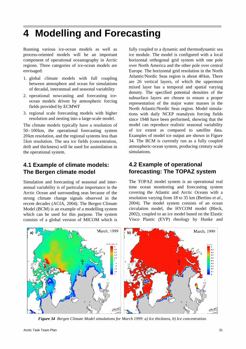
Arctic Task Team Plan 31
Running various ice-ocean models as well asprocess-oriented models will be an importantcomponent of operational oceanography in Arcticregions. Three categories of ice-ocean models areenvisaged: 1. global climate models with full coupling
between atmosphere and ocean for simulationsof decadal, interannual and seasonal variability
2. operational nowcasting and forecasting ice-ocean models driven by atmospheric forcingfields provided by ECMWF
3. regional scale forecasting models with higherresolution and nesting into a large-scale model.
The climate models typically have a resolution of50–100km, the operational forecasting system20km resolution, and the regional systems less than5km resolution. The sea ice fields (concentration,drift and thickness) will be used for assimilation inthe operational system.
4.1 Example of climate models: The Bergen climate modelSimulation and forecasting of seasonal and inter-annual variability is of particular importance in theArctic Ocean and surrounding seas because of thestrong climate change signals observed in therecent decades (ACIA, 2004). The Bergen ClimateModel (BCM) is an example of a modelling systemwhich can be used for this purpose. The systemconsists of a global version of MICOM which is
fully coupled to a dynamic and thermodynamic seaice module. The model is configured with a localhorizontal orthogonal grid system with one poleover North America and the other pole over centralEurope. The horizontal grid resolution in the NorthAtlantic/Nordic Seas region is about 40km. Thereare 26 vertical layers, of which the uppermostmixed layer has a temporal and spatial varyingdensity. The specified potential densities of thesubsurface layers are chosen to ensure a properrepresentation of the major water masses in theNorth Atlantic/Nordic Seas region. Model simula-tions with daily NCEP reanalysis forcing fieldssince 1948 have been performed, showing that themodel can reproduce realistic seasonal variabilityof ice extent as compared to satellite data.Examples of model ice output are shown in Figure34. The BCM is currently run as a fully coupledatmospheric-ocean system, producing century scalesimulations.
4.2 Example of operational forecasting: The TOPAZ systemThe TOPAZ model system is an operational realtime ocean monitoring and forecasting systemcovering the Atlantic and Arctic Oceans with aresolution varying from 18 to 35 km (Bertino et al.,2004). The model system consists of an oceancirculation model, the HYCOM model (Bleck,2002), coupled to an ice model based on the ElasticVisco Plastic (EVP) rheology by Hunke and
4 Modelling and Forecasting
Figure 34 Bergen Climate Model simulations for March 1999: a) Ice thickness, b) Ice concentration.
a) b)

Modelling and Forecasting32
Dukowicz (1997) for the dynamic part. Thermody-namics is computed using a simple parametrisationwith a single ice thickness class (Drange andSimonsen, 1994). The ocean model is forced byatmospheric data, both nowcast and 10–dayforecast with a resolution of 0.5×0.5 degrees,available from the European Center for Mediumrange Weather Forecasting (ECMWF). TheTOPAZ system assimilates weekly fields of sealevel anomalies (SLA) from four satellite altimeters(GFO, ENVISAT, TOPEX–Poséidon, and Jason–2), sea surface temperature (SST) from AVHRR,and sea ice concentrations from SSM/I data. Thedata assimilation method is the Ensemble KalmanFilter (EnKF, Evensen 1994, 2003). Assimilationof ocean surface parameters controls the oceansurface dynamics, as shown by Brusdal et al.(2003) and assimilation of sea ice concentrationshas been developed by Lisæter et al. (2003). Thisenables the model to represent the general circu-lation, such as the Atlantic inflow to the Arctic, soit is well represented in the TOPAZ model. Thenext steps are to assimilate ice drift derived fromsatellite data and drifting ice buoys. Zhang et al.(2003) showed that the assimilation of ice motiondata from SSM/I and buoys improved the icemotion and, through changes in ice motion, the icethickness fields. Every week the TOPAZ systemproduces analysed maps of current ice-ocean state,and 10 day forecasts for the whole Arctic region ata resolution of 20–25km. The sea ice forecastproducts consist of maps of ice concentration, icedrift and ice thickness (Figure 35). Results from themodel systems are provided in several formats,
including presentations on the web(http://www.topaz.nersc.no).
4.3 Ocean Forecasting by the MI–POM model systemThe ocean forecasting system at the NorwegianMeteorological Institute uses the ocean model MI–POM (Engedahl, 1995, 2001), which is based onthe Princeton Ocean Model (Blumberg and Mellor,1987). Lateral forcing includes monthly means ofsea surface elevation, currents, salinity and temper-ature, and fresh and brackish run-off from riversand/or estuaries. MI–POM is fully coupled to thedynamic-thermodynamic sea ice model, MI–IM(Saetra et al., 1999) using the elastic-viscous-plastic (EVP) dynamics of Hunke and Dukowicz(1997) and the thermodynamics of Mellor andKantha (1989). The ice model also handles allfluxes of heat, moisture and momentum from theatmosphere to the ocean in ice-free waters. Atmos-pheric data from the ECMWF are applied asforcing fields.The coupled model system is run once daily toprovide a 10–day forecast of 3–dimensionalcurrent, temperature and salinity, as well as sealevel, ice concentration and ice thickness. Dataassimilation is carried out in a 30–hour run-upperiod. Currently, the operational EUMETSATOSI–SAF SST and sea ice concentration productsare assimilated, using a flux-nudging scheme(Albretsen et al., 2004). Forecast products are madeavailable to users through normal public mediachannels and via met.no’s Ice Service.
Figure 35 Example of forecasted ice drift for the Barents Sea and Fram Strait region on 26 March 2004. Ice drift vectors are calculated and overlaid the ice concentration (greyscale) while the colours show SST in open water.

Arctic Task Team Plan 33
In the current development work a fine-scaleatmosphere-ocean-ice-wave forecast model systemwill be established for the Svalbard area includingassimilation of SAR-based ice observations.Furthermore, the assimilation techniques in ocean-ice models will be improved; a high-resolutionocean-ice model for the Barents Sea will be nestedto the large scale model, and a primary productionecosystem model will be included in cooperationwith the Institute of Marine Research.
4.4 Example of a regional model: the Barents Sea modelA resolution of around 20km, as used in TOPAZ, istoo coarse to resolve mesoscale activity which isvery important for the local representation of iceedge configuration, ice drift and ice concentrationand correspondingly important for the ice thicknessdistribution. Local and detailed sea ice information,including ice thickness, will in future be essential
for safe navigation and operations in these regions.To support these needs a regional high resolution(4km) model for the Barents Sea and the Kara seahas been established using the same ocean and icedynamics as in TOPAZ. For the thermodynamics amore complex ice representation is used whereeach grid cell has several ice thickness classes(Salas, 2002). This ice model also describes theredistribution of ice thickness through ridging andrafting within the grid cell. This coupled ice-oceanmodel uses atmospheric forcing data fromECMWF. The Barents Sea model is nested with the TOPAZsystem. This means that boundary conditions fromthe large-scale models are applied using a one-waynesting scheme where the boundary conditions ofthe regional model are relaxed towards the outputfrom the large-scale model. The Barents Sea modelis presently under validation and is planned to berun in real-time and forecasting mode from 2005.Examples of model output are shown in Figure 37.
Figure 36 Examples of output from met.no’s ice-ocean modelling system: a) ice concentration in %, b) surface temperature in degree C.
a) b)
Figure 37 Examples of Barents Sea model output from test runs for December 2002: a) SST and surface current, b) ice concentration and ice drift.
a) b)

Arctic Task Team Plan 35
The Arctic Task Team will build on a number ofexisting data archiving and distribution systems inthe Arctic Ocean and surrounding seas to provideenvironmental information to a wide range of users.To meet the requirements of all its users it isnecessary to:• identify and make available all data and
products to those organisations adding value tothe products
• provide international communication networksand efficient standard formats and codes tomake best use of them. Such networks andprotocols must have bandwidth sufficient toallow straightforward timely interaction with therelevant data centres.
• implement advanced data quality control andvalidation systems. These systems shouldensure that the large volumes of data requiredand collected are fit for purpose.
• secure archival methods that retain the value ofhistorical data. This requires appropriatecollection, maintenance and dissemination ofdocumentation and metadata.
• establish an integrated international database.For users to locate and recover the informationthey require, the information should be
described in and accessible from advanced dataprocessing systems. These systems aredeveloped and maintained at the individualinstitutions and they will be connected andoperated in a co-ordinated manner, so that infor-mation stored at different sites are as accessibleas if stored in a single location. These systemswill provide a standard set of assessmentmethods allowing investigations of the availa-bility and retrieval of data and products.
• establish link to other data- and modellingcentres for retrieval of boundary and forcingfields. The most urgent and vital part of theArctic Task Team cooperation is the estab-lishment of an efficient system for exchange ofdata between the participating institutions. TheArctic Task Team will basically follow theEuroGOOS Data Policy; but this data policy is,however, primarily focused on operational dataexchange. For the work within the Arctic TaskTeam it is therefore important to establish goodand trustworthy data exchange agreementsbetween the operational and scientificcommunity; since much of the oceanographicwork in the Arctic area is and will be initiatedand funded by the scientific community.
5 Data Exchange
Arctic Task Team Plan 37
Operational oceanography is a growing activity onthe global scale. For the Arctic ocean andsurrounding seas there are presently fewmonitoring and forecasting services in operation,but several new products and services are underdevelopment to serve different users, both interme-diate users and end users. Intermediate users fromthe public and private sectors must be involved inestablishing a feedback loop delivering continuousassessments of the products in terms of accuracy,reliability, and adequacy to their needs. The designof the information delivery system will be formu-lated taking into account their specifications, whichwill allow for specific delivery of information(push) to targeted users, and will plan for easyaccess by a wider class of customers (pull) such asthe scientific community and the general public.Policy makers need simplified informationsummaries in the form of indicators and indices,but presently few such indicators are readilyavailable from the marine environment. The ArcticTask Team will contribute to developing appro-priate indicators on the Arctic marine environment,addressing the objectives and vision of several initi-atives such as GMES, GEO and GCOS.EuroGOOS members already produce a variety ofoperational oceanographic services on a nationalscale of which forecast of sea ice distribution andconcentration, wave forecasts, drift forecasts arethe most advanced. These services are distributedto the users via established communication lines(phone, fax), Internet, and public media (papers,radio, TV). It is obvious that no operational crossboundary system in any domain can be successfulwithout an efficient and robust informationexchange and dissemination system. It is even moreobvious that systems relying on data collected indifferent parts of the Arctic area by different partiescannot become really operational without such aninformation system.Parallel to the improvement and development ofoperational oceanographic activities in the Arctic it
is important to promote the products and servicesgenerated by the Arctic TT members throughawareness campaigns addressing a full hierarchy ofstakeholders. Governmental agencies and author-ities, policy-makers, the marine scientificcommunity, and the marine industries and servicessector will be the main target. The campaigns willtake an outset in the contacts and the lessons learntin previous and present EuroGOOS activities andEU funded projects. The purpose will be to buildmomentum towards societal support and seekcommitment from governments for operationalocean monitoring and forecasting. The Arctic Taskteam will work in close cooperation with the Inter-national Polar Year 2007–2008 which offers aunique opportunity to promote monitoring andforecasting in the Arctic regions. The specific objectives of the dissemination systemfor the Arctic Ocean and surrounding seas are to1. prepare promotional material on operational
oceanography products based on existingmaterial from the Arctic Task Team
2. develop, validate and demonstrate new productsto various users from industry, government,international programmes and other user groups
3. demonstrate through a cost benefit analysis theadvantages of operational ocean forecastproducts available for a range of services andthereby develop a market for such products
4. plan and coordinate marketing activities for theArctic Task Team
5. establish networks between operational serviceproducers, value-added service providers andend-users.
6. identify existing and possible expansion of themarkets for operational oceanography in polarregions
7. establish and run a web site for the Arctic TaskTeam for promotion and exchange of infor-mation.
6 Dissemination

Arctic Task Team Plan 39
ACIA (2004). Impacts of a warming Arctic: Arctic Climate Impact Assessment, November, 2004(http://amap.no/acia/).
Albretsen, J. (2004). Operational use of regional high-resolution sea surface temperature and sea ice concen-tration in a coupled sea ice and ocean model. Submitted to Journal of Marine Systems.
Alexandrov, V.Yu., S. Sandven, O.M. Johannessen, Ø. Dalen and L.H. Pettersson (2000). Winter navigationin the Northern Sea Route. Polar Record, Vol. 36 (199), 333–342.
Alekseev, G., O.M. Johannessen, A. Korablev, V. Ivanov, D. Kovalevsky (2000). Interannual variability ofwater masses in the Greenland Sea and adjacent areas. The Sverdrup symposium, Journal of theNorwegian Polar Research vol. 20, no.2, 2001, pp. 201–208.
AMAP (2003), AMAP Assessment (2002). The influence of Global Change on Contaminant Pathways to,within, and from the Arctic, Oslo 2003, 65 pp (http://amap.no).
ASOF (2000). Strawman-3, Science Plan for the Arctic-Subarctic Ocean Flux Array, part A, B, C and D (ed.B. Dickson), October 2000 (available at http://asof.npolar.no).
ASOF (2002). ASOF Implementation Plan, version 2, April 2002 (http://asof.npolar.no).
Barlindhaug, J.P. (2004). Seminar at Norwegian Petroleum Association, Bergen, 26–28 January, 2004.
Bertino (2004), with Lisæter, Sagen, Counillon, Winther, Stette, Natvik, G. Evensen, Morel, Brankart, Testut,Birol, Brasseur, Verron, Schartau,, Schröter, Dombrowsky, Burillo, Gilles Larnicol, Schaeffer andWeller. Towards an Operational Prediction system for the North Atlantic and European coastalZones—TOPAZ Final report, NERSC Technical Report, 251.
Bleck (2002). An oceanic general circulation model framed in hybrid isopycnic–Cartesian coordinates. OceanModelling, Vol.4,pg 55–88.
Blumberg, A.F., and G.L. Mellor (1988). A description of a three-dimensional coastal ocean circulationmodel. In: Three-Dimensional Coastal Ocean Models, ed. N.S. Heaps, AGU Coastal and EstuarineSer., 4, American Geophysical Union, Washington D.C.
Bratseth, A.M. (1986). Statistical interpolation by means of successive corrections. Tellus, 38A, 439–447.
Breivik, L.A., and M. Reistad (1994). Assimilation of ERS–1 altimeter wave heights in an operationalnumerical wave model. Weather and Forecasting, 9(3).
Brusdal, K., J.M. Brankart, G. Halberstadt, G. Evensen, P. Brasseur, P.J. van Leeuwen, E. Dombrowsky andJ. Verron (2003). A demonstration of ensemble based assimilation methods with a layered OGCM fromthe perspective of operational ocean forecasting systems, Jour. Mar. Systems, 40–41, pp. 253–289.
Commission of the European Communities (2004). Global Monitoring for Environment and Security(GMES): Establishing a GMES capacity by 2008—(Action Plan (2004–2008)). Communication fromthe Commission to the European Parliament and the Council, COM (2004) 65 Final, 23 pp.
Bönisch, G., J. Blinheim, J.L. Bullister, P. Schlosser, and D.W.R. Wallace (1997). Long-term trends oftemperature, salinity, density and transient tracers in the central Greenland Sea. Journal of GeophysicalResearch, 102 (C8), 18553–18572.
Cochran, J.K., D.J. Hirschberg, H.D. Livingston, K.O. Buesseler, and R.M. Key (1995). Natural and anthro-pogenic radionuclide distributions in the Nansen Basin, Arctic Ocean: scavenging rates and circulationtimescales. Deep Sea Research, II, 42 (6), 1495–1517.
D.F. Dickins Associates Ltd. (2004). Advancing Oil Spill Response in ice-covered waters, 18 pp. PrinceWilliam Sound Oil Spill Recovery Institute, Cordova, Alaska, USA (www.pws-osri.org)
7 References
References40
Dickson, B., Yashayaev, Meincke, Turrell, Dye and Holfort (2002). Rapid freshening of the deep NorthAtlantic Ocean over the past four decades. Nature, 416.
Dickson, B. (ed.) (2004), The Northern Seas at a time of Global Change: an AOSB–CLIC observing plan forIPY, 91 pp.
Drange and Simonsen (1996). Formulation of air-sea fluxes in ESOP2 version of MICOM, Technical report125, Nansen Environmental and Remote Sensing Center, Bergen, Norway.
Engedahl, H. (1995). Implementation of the Princeton Ocean Model (POM/ECOM3D) at the NorwegianMeteorological Institute. Res. Rep. No. 5, Norwegian Meteorological Institute, Oslo, Norway.
Engedahl, H. (2001). Operational ocean models at Norwegian Meteorological Institute. Research Note No.59, Norwegian Meteorological Institute, Oslo, 26 pp.
Evensen (1994). Sequential data similation with a nonlinear quasi-geostropic model using Monte carlomethods to forecast error statisitics. J. Geophys. Res., 99, 10143–10162.
Evensen (2003). The Ensemble Kalman Filter: theoretical formulation and practical implementation, OceanDynamics, Vol.53, pp. 343–367.
Ezraty, R. and J.F. Piollé (2003). Sea Ice drift in the Arctic, User’s manuals, http://www.ifremer.fr/cersat.
Franke, M., W.M. Smethie Jr. and R. Bayer (1998). Investigation of subsurface water flow along the conti-nental margin of the Eurasian Basin using the transient tracers tritium, 3He and CFCs. Journal ofGeophysical Research, 103, 30773–30792.
Frantzen, B. and A. Bambuliak (2003). Oil transport from the Russian part of the Barents Region. Report fromSvanhovd Environmental Centre to the Barents Secretariat, Norway, July 2003 (http://www.barsek.no).
Gascard, J.-C., A.J. Watson, M.-J. Messias, K.A. Olsson, T. Johannessen, and K. Simonsen, (2002).Longlived vortices as a mode of deep ventilation in the Greenland Sea. Nature, London, 416, 525–527.
GCOS (2004). Implementation Plan for the Global Climate Observing System for Climate in Support of theUnited Nations Framework Convention on Climate Change, Final draft, 20 September, 2004, 130 pp.
Global Monitoring for Environment and Security (2004). Final Report from the GMES Initial Period (2001–2003) from the GMES Steering Committee, 10 February 2004, 44 pp. (http://gmes.info).
Guay, C.K. and K.K. Falkner (1997). Barium as a tracer of Arctic halocline and river waters. Deep SeaResearch II, 44 (8), 1543–1569.
Gould, J. and the Argo Steering Team (2004). Argo Profiling Floats Bring New Era of In Situ Ocean Obser-vations, EoS Vol. 85, No. 19, May 2004.
Haas, C., and H. Eicken (2001). Interannual variability of summer sea ice thickness in the Siberian andCentral Arctic under different atmospheric circulation regimes, J. Geophys. Res., 106(C3), 4449–4462.
Haine, T.W.N., A.J. Watson, and M.I. Liddicoat, (1995). Chlorofluorocarbon in the Northeast Atlantic.Journal of Geophysical Research, 100 (C6), 10745–10753.
Hansen, B. and S. Österhus, (2000). North Atlantic-Nordic Seas exchanges, Prog. in Oceanography, 45:109–208.
Hansen, Turrell and Österhus (2001). Decreasing overflow from the Nordic Seas into the Atlantic Oceanthrough the Faroe–Shetland Channel since 1950, Nature, 411, 927–930.
Harder, M., and H. Fischer (1999). Sea ice dynamics in the Weddell Sea simulated with an optimized model,J. Geophys. Res., 104(C5), 11151–11162.
Heinze, C., E. Maier-Reimer, and P. Schlosser (1998). Transient tracers in a global OGCM: source functionsand simulated distributions. Journal of Geophysical Research, 103 (C8), 15903–15922.
Hunke, E.C., and Dukowicz, J.K. (1997). An elastic-viscous-plastic model for sea ice dynamics. J. Phys.Oceanogr., 27, 1849–1867.
IGOS (2004). Concept of an IGOS-Cryosphere Theme (IGOS-Cryo), October 2004.

Arctic Task Team Plan 41
International Maritime Organisation (2002). Guidelines for ships operating in Arctic ice-covered waters,MSC/Circ. 1056 MEPC/Circ.399, December 2002, 33 pp.
International Polar Year (2004). A framework for the International Polar Year, October 2004, 74 pp,www.ipy.org.
JCOMM Polar Observations (2000). A Report to the WMO/IOC Joint Commission on Oceanography andMarine Meteorology, first draft April 2000, 78 pp.
Jenkins, W.J. (1988). The use of anthropogenic tritium and helium-3 to study sub-tropical gyre ventilationand circulation. Phil. Trans. Royal Soc. London, A325, 43–61.
Johannessen, O.M., E.V. Shalina and M.W. Miles (1999). Satellite Evidence for an Arctic Sea Ice cover inTransformation. Science, 286, 1937–1939.
Johannessen, O M., A.M. Volkov, L.P. Bobylev , V.D. Grischenko, S. Sandven, L.H. Pettersson, V.V.Melentyev, V. Asmus, O.E. Milekhin, V.A. Krovotyntsev, V.G. Smirnov, V.Yu. Alexandrov, G.Duchossois, V. Kozlov, G. Kohlhammer and G. Solaas. (2000). ICEWATCH—Real-time sea icemonitoring of the Northern Sea Route using satellite radar (a Cooperative Earth Observation Projectbetween the Russian and European Space Agencies). Earth Observation and Remote Sensing, Vol. 16,No. 2, 257–268.
Johannessen, O.M., M.W. Miles, L. Bengtsson, L.P. Bobylev and S.I. Kuzmina (2003). Arctic climatechange, In Arctic Environment Variability in the Context of Global Change (eds. Bobylev, L.P., K.Ya.Kondratyev and O.M. Johannessen), Springer–Praxis Publishing, 470 pp.
Johannessen, J.A., G. Bamino, C. Le Provost, R. Rummel, R. Sabadini, H. Sunklel, C.C. Tscherning, P.Visser, P. Woodworth, C.W. Hughes, P. Legrand, N. Sneeuw, M. Aguirre–Martinez, H. Rebhan andM. Drinkwater (2003). The European Gravity Field and Steady-State Ocean Circulation ExplorerSatellite Mission: Its impact on geophysics. Surveys in Geophysics, 24, 339–386.
Johannessen, O.M. (2004a). Arctic climate change: observed and modeled temperature and sea-ice varia-bility. Tellus, Series A: Vol.56A, no.4, July 2004.
Johannessen, O.M. et al. (2004b). Climate of the Arctic and its Role for Europe (CARE)—a Europeancomponent of the International Polar Year. Workprogramme for a Specific Support Action funded byEU's Sixth Framework Programme, 44 pp.
Karcher, M.J., S. Gerland, I.H. Harms, M. Iosjpe, H.E. Heldal, and P.J. Kershaw (2002). The dispersion of99Tc in the Nordic Seas and the Arctic Ocean in the 1990s according to model results and observations.Proc. Int. Conf. Radioactivity in the Environment, Monaco, 511–515.
Karcher, M., R. Gerdes, F. Kauker, and C. Köberle (2003). Arctic warming: Evolution and spreading of the1990s warm event in the Nordic Seas and the Arctic Ocean. J. Geophys. Res., C2, 108, 3034.
Kershaw, P.J. and A. Baxter (1995). The transfer of reprocessing wastes from north-west Europe to theArctic. Deep Sea Research II, 42 (6), 1413–1448.
Kwok, R. (1998). The RADARSAT Geophysical Processor System. In Tsatsoulis and Kwok (eds.) Analysisof SAR Data of the Polar Oceans. Springer Verlag, pp. 235–257.
Laxon, S., N. Peacock and D. Smith (2003). High interannual variability of sea ice thickness in the Arcticregion. Nature, Vol. 245, pp. 947–950.
Lal, D. (1999). An overview of five decades of studies of cosmic ray produced nuclides in the oceans. Scienceof the Total Environment, 237/238, 3–13.
Law, C.S., A.P. Martin, M.I. Liddicoat, A.J. Watson, K.J. Richards,. and E.M.S. Woodward (2001). ALagrangian SF6 tracer study of an anticylonic eddy in the North Atlantic: patch evolution, verticalmixing and nutrient supply to the mixed layer. Deep Sea Research II, 48, 705–724.
Ledwell, J.R., A.J. Watson, and C.S. Law (1993). Evidence for slow mixing across the pycnocline from anopen ocean tracer release experiment. Nature, London, 364, 701–703.

References42
Lisæter, K.A., J. Rosanova, and G. Evensen (2003). Assimilation of ice concentration into a coupled ice-ocean model, using the Ensemble Kalman Filter, Ocean Dynamics, 53: 368–388.
Mellor, G.L., and L. Kantha (1989). An ice-ocean coupled model. J. Geophys. Res. 94, 10937–10954.
Moran, S.B., K.M. Ellis, and J.N. Smith (1997). 234Th/238U disequilibrium in the central Arctic Ocean:implications for particulate organic carbon export. Deep Sea Research II, 44 (8), 1593–1606.
Morison, J., M. Steele and Andersen (1998). Hydrography of the upper Arctic Ocean measured from thenuclear submarine USS Pargo, Deep-Sea Res. I, 45, 15–38.
Morison, J.H., K. Aagaard and M. Steele (2000). Recent Environmental Changes in the Arctic: A review.Arctic, 53, 4.
Murata, A. and T. Takizawa (2003). Summertime CO2 sinks in shelf and slope waters of the western ArcticOcean. Continental Shelf Research, 23, 753–776.
Oliver and Heywood (2003). Heat and freshwater fluxes through the Nordic Seas, J. Phys. Oceanog., 33,1009–1026.
PAME (2000). PAME—Snap Shot Analysis of Maritime Activities in the Arctic, Norwegian Maritime Direc-torate Report no. 2000–3220, 72 pp.
PAME (2002). Arctic Offshore Oil and Gas Guidelines, Report form the Arctic Council Working Group:Protection of the Arctic Marine Environment, October 2002, 82 pp.
Peterson, B.J., R.M. Holmes, J. McClelland, C.J. Vörösmarty, R.B. Lammers, A.I. Shiklomanov, I.A.Shiklomanov, and S. Rahmsdorf (2002). Increasing river discharge to the Arctic Ocean. Science 298(13 December 2002), 2171–2173.
Peterson, C.H., S.D. Rice, J.W. Short, D. Esler, J.L. Bodkin, B.E. Ballachey, and D.B. Irons (2003). Long-Term Ecosystem Response to the Exxon Valdez Oil Spill, Science, Vol. 302, 2082–2086.
Pettersson, L.H., S. Sandven, Ø. Dalen, V.V. Melentyev and N.I. Babich (1999). Satellite radar icemonitoring for ice navigation of the ARCDEV tanker convoy in the Kara Sea. Proceedings of The 15thInternational Conference on Port and Ocean Engineering under Arctic Conditions, Helsinki, Finland,August 23–27, 1999, pp. 141–153.
Rothrock, D.A., Y. Yu, and G.A. Maykut (1999). Thinning of the Arctic Sea-Ice Cover. Geophys. Res. Lett.23, 23, 3469–3472.
Salas (2002). A global coupled sea-ice ocean model, Ocean modelling,4, p. 137–172.
Sandven, S., A. Seina, H. Gronvall, H.H. Valeur and H. Steen Andersen (1999). OSIMS—Operational SeaIce Monitoring by Satellites in Europe. Proceedings of The 15th International Conference on Port andOcean Engineering under Arctic Conditions, Helsinki, Finland, August 23–27, 1999. pp. 508–517.
Sandven, S., Ø. Dalen, M. Lundhaug, K. Kloster, V.Y. Alexandrov, and L.V. Zaitsev (2001). Sea ice investi-gations in the Laptev Sea area in late summer using SAR data. Canadian Journal of Remote Sensing,vol. 27, no. 5, 502–516.
Schlosser, P., J.H. Swift, D. Lewis, and S.L. Pfirman (1995). The role of the large-scale Arctic Ocean circu-lation in the transport of contaminants. Deep Sea Research II, 42 (6), 1341–1367.
Schlosser, P., R. Bayer, G. Bönisch, L.W. Cooper, B. Ekwurzel, W.J. Jenkins, S. Khatiwala, S. Pfirman, andW.M. Smethie (1999). Pathways and mean residence times of dissolved pollutants in the ocean derivedfrom transient tracers and stable isotopes. Science of the Total Environment, 237/238, 15–30.
Smethie Jr., W.M., P. Schlosser, and G. Bönisch (2000). Renewal and circulation of intermediate waters inthe Canadian Basin observed on the SCICEX 96 cruise. Journal of Geophysical Research, 105 (C1),1105–1121.
Smith, J.N. and K.M. Ellis (1995). Radiotracer tracer profiles at the CESAR Ice Station and Canadian IceIsland in the western Arctic Ocean, Deep Sea research, II, 42 (6), 1449–1470.

Arctic Task Team Plan 43
Smith, J.N., K.M. Ellis, and T. Boyd (1999). Circulation features in the central Arctic Ocean revealedbynuclear fuel reprocessing tracers from Scientific Ice Expeditions 1995 and 1996. Journal ofGeophysical Research, 104 (C12), 29663–29677.
Rhein, M. (1991). Ventilation rates of the Greenland and Norwegian Seas derived from distributions of thechlorofluoromethanes F11 and F12. Deep Sea Research, 38 (4), 485–503.
Semenov, V.A. and L. Bengtsson (2003). Wintertime Arctic temperature variability in the 20th century:dominant modes. EGS–AGU–EUG Joint Assembly, Nice, France, 6–11 April 2003, Geophys. Res.Abstracts, vol. 5 (CD–ROM), 2003.
Shiklomanov, I.A., A.I. Shiklomanov, R.B. Lammers, B.J. Peterson, and C.J. Vörösmarty (2000). In TheFreshwater Budget of the Arctic Ocean (Ed. E. L. Lewis), Kluwer Academic, Dordrecht, Netherlands,2000, pp. 281–296.
Steele, M. and T. Boyd (1998). Retreat of the cold halocline layer in the Arctic Ocean. J. Geophys. Res. 103,p. 10419–10435.
Sætra, Ø., L.P. Røed and J. Albretsen (1999). The DNMI Regclim ice model. Tech. Rep. 3, RegClim GeneralTechnical Report, Norwegian Meteorological Institute, Oslo.
Tao, X., J.E. Walsh, and W.L. Chapman (1996). An assessment of global climate model simulations of Arcticair temperatures, J. Climate, 9, 1060–1076.
Thoresen, R. and O.J. Østvedt (2000). Variations in the abundance of Norwegian spring-spawning herring(Clupea harengus, Clupeidae) throughout the 20th century and the influence of climatic fluctuations.Fish and Fisheries 1: 231–256.
Turell, W.R., G. Slesser, R.D. Adams, R. Payne, and P.A. Gillibrand (1999). Decadal variability in FaroeShetland Channel Bottom Water, Deep-Sea Res. 46: 1–25.
Vinje, T., N. Nordlund, and A. Kvambekk (1998). Monitoring ice thickness in Fram Strait, J. Geophys. Res.,103(C5), 10437–10449.
Wadhams, P. (1994). Sea ice thickness changes and their relation to climate. In O.M. Johannessen et al. (eds.)The Polar Oceans and Their Role in Shaping the Global Environment, Geophysical Monograph 85,American Geophysical Union, Washington DC, 337–361.
Watson, A.J., M-J. Messias, E. Fogelqvist, K.E. van Scoy, T. Johannessen, K.I.C. Oliver, D.P. Stevens, F.Rey, T. Tanhua, K.A. Olsson, F. Carse, K. Simonsen, J.R. Ledwell and E. Gullyardi (1999). Mixingand convection in the Greenland Sea from a tracer-element experiment. Nature, London, 401 (6756),902–904.
Zhang, Thomas, Rothrock, Lindsay, and Yu (2003). Assimilation of ice motion observations and comparisonswith submarine thickness data. J. Geophys.Res. Vol. 108, C6.
Östlund, H.G. and G. Hut (1984). Arctic Ocean water mass balance from isotope data. Journal of PhysicalOceanography, 89, 6373–6381.
Österhus, S., B. Hansen, R. Kristiansen, and P. Lundberg (1999). The Atlantic Water inflow to the NordicSeas, The International WOCE Newsletter, 35:35–37.
Österhus and Gammelsrød (1999). The abyss of the Nordic Seas is warming, Journal of Climate, 12(11),3297–3304.

Arctic Task Team Plan 45
List of contributors to this report
8 Contributors
Arctic Task Team Plan 47
To be updated or removedA. Ice strengthened Research Ships and Ice
Breakers A basic component to measure in situ data areresearch vessels. They supply data from ship-bornerepeat surveys, and are needed to deploy andrecover moored instruments, as well as deploy andeventually recover autonomous floats and vehicles.Ice breaking research vessels will be the backboneof an Arctic measurement system, even if airdeployments will play a role as well.List of available and planned vessels with icecapabilityGermanyPOLARSTERN, research ice breaker in service NN, Medium size vessel for ice margin use inadvanced planning phaseAURORA BOREALIS, plans as European icebreaker with all year round operation facilitiesNorwayLANCE, research vessel for the marginal ice zonein service
NN, Plans for a ice breaker in an less advancedstatusSwedenODEN, ice breaker available for 180 days duringthe next 3 to 5 yearsUKJAMES CLARK ROSS, research vessel for themarginal ice zone in serviceSHACKLETON, ice breaker available on multi-year commitment
Canada CCGS LOUIS S. St-LAURENT, Ice breaker butnot budget committedUSAUSCGC HEALY, Ice breaker in even years inwestern Arctic, in odd years in eastern ArcticAdditionally Russian vessels and military subma-rines are available to a certain extent. However, asustained observation system requires to considerthe further development of the research fleet andappropriate new vessels have to be build.
9 Appendix