Eulerian Solid-Fluid Coupling

Yun Teng∗ David I.W. Levin† Theodore Kim∗‡

∗University of California, Santa Barbara †Disney Research ‡Pixar Animation Studios

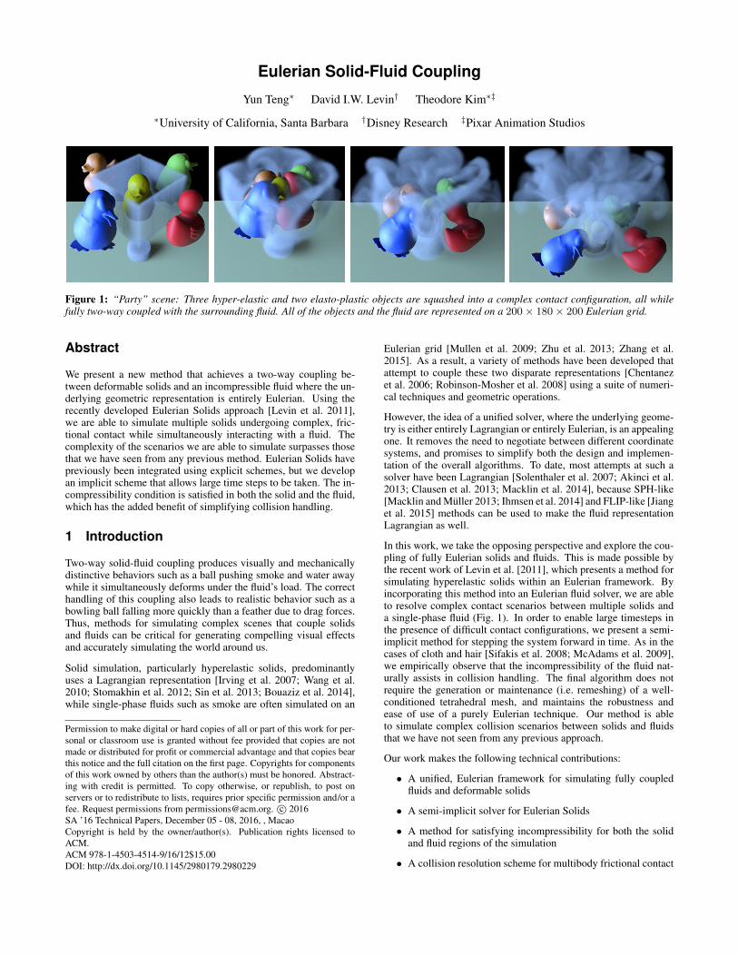
Figure 1: “Party” scene: Three hyper-elastic and two elasto-plastic objects are squashed into a complex contact configuration, all whilefully two-way coupled with the surrounding fluid. All of the objects and the fluid are represented on a 200× 180× 200 Eulerian grid.

Abstract

We present a new method that achieves a two-way coupling be-tween deformable solids and an incompressible fluid where the un-derlying geometric representation is entirely Eulerian. Using therecently developed Eulerian Solids approach [Levin et al. 2011],we are able to simulate multiple solids undergoing complex, fric-tional contact while simultaneously interacting with a fluid. Thecomplexity of the scenarios we are able to simulate surpasses thosethat we have seen from any previous method. Eulerian Solids havepreviously been integrated using explicit schemes, but we developan implicit scheme that allows large time steps to be taken. The in-compressibility condition is satisfied in both the solid and the fluid,which has the added benefit of simplifying collision handling.

1 Introduction

Two-way solid-fluid coupling produces visually and mechanicallydistinctive behaviors such as a ball pushing smoke and water awaywhile it simultaneously deforms under the fluid’s load. The correcthandling of this coupling also leads to realistic behavior such as abowling ball falling more quickly than a feather due to drag forces.Thus, methods for simulating complex scenes that couple solidsand fluids can be critical for generating compelling visual effectsand accurately simulating the world around us.

Solid simulation, particularly hyperelastic solids, predominantlyuses a Lagrangian representation [Irving et al. 2007; Wang et al.2010; Stomakhin et al. 2012; Sin et al. 2013; Bouaziz et al. 2014],while single-phase fluids such as smoke are often simulated on an

Permission to make digital or hard copies of all or part of this work for per-sonal or classroom use is granted without fee provided that copies are notmade or distributed for profit or commercial advantage and that copies bearthis notice and the full citation on the first page. Copyrights for componentsof this work owned by others than the author(s) must be honored. Abstract-ing with credit is permitted. To copy otherwise, or republish, to post onservers or to redistribute to lists, requires prior specific permission and/or afee. Request permissions from permissions@acm.org. c© 2016SA ’16 Technical Papers, December 05 - 08, 2016, , MacaoCopyright is held by the owner/author(s). Publication rights licensed toACM.ACM 978-1-4503-4514-9/16/12$15.00DOI: http://dx.doi.org/10.1145/2980179.2980229

Eulerian grid [Mullen et al. 2009; Zhu et al. 2013; Zhang et al.2015]. As a result, a variety of methods have been developed thatattempt to couple these two disparate representations [Chentanezet al. 2006; Robinson-Mosher et al. 2008] using a suite of numeri-cal techniques and geometric operations.

However, the idea of a unified solver, where the underlying geome-try is either entirely Lagrangian or entirely Eulerian, is an appealingone. It removes the need to negotiate between different coordinatesystems, and promises to simplify both the design and implemen-tation of the overall algorithms. To date, most attempts at such asolver have been Lagrangian [Solenthaler et al. 2007; Akinci et al.2013; Clausen et al. 2013; Macklin et al. 2014], because SPH-like[Macklin and Muller 2013; Ihmsen et al. 2014] and FLIP-like [Jianget al. 2015] methods can be used to make the fluid representationLagrangian as well.

In this work, we take the opposing perspective and explore the cou-pling of fully Eulerian solids and fluids. This is made possible bythe recent work of Levin et al. [2011], which presents a method forsimulating hyperelastic solids within an Eulerian framework. Byincorporating this method into an Eulerian fluid solver, we are ableto resolve complex contact scenarios between multiple solids anda single-phase fluid (Fig. 1). In order to enable large timesteps inthe presence of difficult contact configurations, we present a semi-implicit method for stepping the system forward in time. As in thecases of cloth and hair [Sifakis et al. 2008; McAdams et al. 2009],we empirically observe that the incompressibility of the fluid nat-urally assists in collision handling. The final algorithm does notrequire the generation or maintenance (i.e. remeshing) of a well-conditioned tetrahedral mesh, and maintains the robustness andease of use of a purely Eulerian technique. Our method is ableto simulate complex collision scenarios between solids and fluidsthat we have not seen from any previous approach.

Our work makes the following technical contributions:

• A unified, Eulerian framework for simulating fully coupledfluids and deformable solids

• A semi-implicit solver for Eulerian Solids

• A method for satisfying incompressibility for both the solidand fluid regions of the simulation

• A collision resolution scheme for multibody frictional contact

2 Related Work

Beginning with the immersed boundary method [Peskin 1972], sim-ulating the coupled motion of solids and fluids has a long history inboth graphics and engineering. In graphics, there has been muchwork coupling fluids to rigid bodies [Takahashi et al. 2002; Carlsonet al. 2004; Klingner et al. 2006; Batty et al. 2007], as well as rigidand deformable shells [Guendelman et al. 2005].

Chentanez et al. [2006] modeled the deformable solid as an unstruc-tured tetrahedral mesh and showed how to couple it to an Eulerianfluid, which could be represented as either a regular grid or an-other unstructured mesh. This approach requires a mesh generationstage, and the specific formulation required an asymmetric systemto be solved. This approach has been extended to fully Lagrangiansimulations of both the solid and fluid [He et al. 2012; Souli andBenson 2013; Wick 2013], and has incorporated additional phe-nomena such as phase transitions [Clausen et al. 2013] and porousflow [Lenaerts et al. 2008]. Other methods have further investigatedEulerian fluid discretizations and used sophisticated geometric op-erations [Robinson-Mosher et al. 2008; Robinson-Mosher et al.2009] as well as overlapping grids [Baaijens 2001] to couple thegrid velocities to a Lagrangian solid. Fast, approximate, position-based methods have also been recently developed for real-time ap-plications [Macklin et al. 2014], which can often need careful pa-rameter tuning to generate realistic results.

Recently, the Material Point Method (MPM) [Stomakhin et al.2014; Jiang et al. 2015] has become popular for simulating a num-ber of mixed-phase phenomena. It shares some of the same advan-tages of our approach, as it avoids the need for complex remeshingschemes and geometric conversions. However, as mentioned byJiang et al. [2016], these schemes are known to have issues rep-resenting hyperelastic materials, as artificial plasticity can creepinto the simulation. Our scheme naturally handles hyperelastic re-sponse, even in the presence of a fluid, and still allows the user toadd plasticity if desired.

In order to avoid complicated meshing schemes, simulate elas-tic objects accurately, and robustly resolve complicated collisions,Levin et al. developed the Eulerian Solids methodology [2011].With this technique in hand, it is natural to ask whether we can nowperform solid-fluid coupling in a purely Eulerian fashion. The clos-est work to ours in the engineering literature is Kamrin et al. [2012],which showed that a similar “reference map” method can be usedto couple deformable, elastic solids to weakly compressible flu-ids. The approach has also been extended to handle non-frictionalcontact between two objects [Valkov et al. 2015]. However, thismethod does not handle incompressible fluids, large time steps orcomplex contacts between a multitude of objects. Crucially, theirefficacy has also only been demonstrated on coarse 2D grids. Incontrast, we present a fully 3D Eulerian Solids-based solver thatcouples an incompressible fluid to multiple deformable objects un-dergoing frictional contact. By using an implicit time integrationscheme, we are able to take large timesteps.

3 Eulerian Solid and Fluid Preliminaries

Notation: We will denote vectors using bold lowercase, e.g. f , andmatrices using bold uppercase, e.g. M. Unbolded symbols repre-sent scalars. Departing from the usual fluid simulation notation, weuse u to represent the displacement field of a solid object and in-stead use v for velocity. A superscript to the left of a variable isused to distinguish solid objects from fluid. Unlabelled vectors areconsidered global, i.e. they contain both solid and fluid entries. Asuperscript ? denotes intermediate states prior to advection, and anoverbar, e.g. x denotes the reference configuration of variable x.

Eulerian Solids: In the interest of self-containment, we will givea brief overview of Eulerian Solids, but full details can be foundin previous work [Levin et al. 2011; Fan et al. 2013]. The firststep of any continuum simulation of materials is to discretize thedeformation mapping, φ : x → x from material space to physicalspace. Eulerian Solids discretize the physical space as a regular gridand store the material space coordinates as a field to be advected.Rather than store the full material coordinates, we follow Fan etal. [2013], and advect the displacement field u, which improves therobustness of the method under large time steps.

The advected u is the key to the Eulerian solids approach, as itallows the direct computation of the deformation gradient F using

F =

(I− ∂u

∂x

)−1

. (1)

With this F, we can compute the forces inside a solid using any ar-bitrary constitutive model. Crucially, only displacement fields withzero deformation can yield F = I. This guarantees that an elas-tic constitutive model will always generate forces that attempt toreturn to a zero deformation state, and ensure an accurate hyper-elastic simulation.

Eulerian Fluids: For completeness, we also give a brief overviewof fluids, but more details can be found in Bridson [2008]. Theequations for an inviscid, incompressible fluid are:

∂v

∂t+ v · ∇v +

1

ρ∇p = g,

∇ · v = 0.

(2)

The first equation is the momentum equation and the second is theincompressibility constraint. Here, v is the velocity of the fluid, ρit the density, p the pressure, and g denotes external forces such asgravity.

Approximating the derivatives using Eulerian finite differences isstraightforward, which makes them a popular method for simulat-ing fluids. A basic solver is as follows:

∂v

∂t+ v · ∇v = 0, (3)

∂v

∂t= g, (4)

∂v

∂t+

1

ρ∇p = 0 such that ∇ · v = 0. (5)

Eqn. 4 adds the body forces and is often integrated explicitly.Eqn. 5 is usually solved using a Helmholtz-Hodge decompositionthat projects out the divergent component of the velocity, and typi-cally requires the solution of a Poisson problem.

The advection step, Eqn. 3, plays a key role in the stability ofthe simulation. Semi-Lagrangian [Stam 1999] and Fluid-Implicit-Particle (FLIP) [Brackbill and Ruppel 1986; Jiang et al. 2015]methods are two widely used schemes. The former is performedentirely on the Eulerian grid while the latter relies on auxiliary La-grangian particles.

4 Coupled Solid–Fluid Simulation

4.1 The Continuous Formulation

In this work we focus on the coupled simulation of multiple in-compressible, hyper-elastic, and elasto-plastic solids immersed in

an incompressible fluid. This requires us to solve the momentumequation, given by

ρdv

dt= ∇ · σ + f

∇ · v = 0

∀x ∈ Ω

fv = sv ∀x ∈ Γ

(6)

where Ω denotes a region in world space, x denotes a point in worldspace, v is the velocity of a particle at x, σ is the Cauchy stress andf are external forces such as gravity. For each x containing a solid,we compute σ using a standard hyper-elastic or elasto-plastic con-stitutive model, and for each x containing a fluid we set σ = 0. Forthese cells, the divergence-free condition, ∇ · v = 0, is sufficient.We also enforce a no slip condition along the solid-fluid boundaryΓ, where fluid and solid velocities are respectively denoted fv andsv. We use the hyper-elastic model of McAdams et al. [2011] forthe elastic component of all of our examples.

Figure 2: The high-level structure of our data storage and compu-tation scheme. To assist advection and contact handling, we keepseparate velocity fields for each solid object. For efficiency, onlyvalues near the solid are updated.

4.2 Spatial Discretization and Constraints

Our method relies on fixed discretizations of both x and x. In or-der to solve Eqn. 6, we discretize Ω using regular, hexahedral fi-nite elements. Velocity, displacement and forces are co-located atthe grid nodes, while pressure values is stored at grid centers. Inorder to incorporate equality constraints we rely on a mixed formu-lation in which incompressibility is applied as a point constraint atthe cell center. This can be considered an under-integrated finiteelement, which is commonly used to prevent locking [Belytschkoet al. 2013]. We then compute per-element mass and stiffness matri-ces, based on whether each cell contains a solid or a fluid, using aneight-point quadrature rule, and then assemble into global M and Koperators. Our discretized divergence-free constraint is expressedas Jv = 0 where J is the constant constraint gradient. Note thatdue to the continuity of the velocity field, the no slip condition onsolid-fluid boundaries is implicitly enforced, and no special spatialcoupling terms need to be formulated.

To facilitate velocity advection and collision detection, each solidstores a copy of the velocity field, but only values near the solid areever updated. Fig. 2 shows our high level data storage and compu-tation structure. Our algorithm also requires a discretization of x ifplastic deformation is desired. For each plastic solid, we create anauxiliary grid of that solid’s reference coordinate system lx, wherel ∈ [1, Ns] indexes each solid in the simulation.

4.3 Time Integration

We use a splitting scheme to advance our system in time. First,we use implicit integration to compute a divergence-free velocityfield for the solid cells, and then perform an advection that resolvescollisions. Algorithm 1 gives an overview of our time integrationscheme. In the next sections, we describe the key components ofour algorithm: a semi-implicit update for Eulerian Solids, pressureprojection, and a collision resolution scheme.

Algorithm 1 Eulerian solids and fluids simulation

1: Compute ∆t based on CFL condition2: for each solid object, l do3: Compute mass lM and volume fraction lV on the grid4: Compute material force lf and stiffness matrix lK5: . (§4.4)6: end for7: Compute fluid mass fM8: Assemble M, K, C and f? . (§4.4)9: v? = G−1f? . (Eqn. 8)

10: Compute pressure p . (Eqn. 12)11: Pressure project v? to get pre-advection vn+1 . (Eqn. 13)12: for each solid object, l do13: Update solid particle velocities using FLIP from lvn+1

14: Add repulsions and frictions to particles in collision15: . (§4.6)16: end for17: for each solid object, l do18: Rasterize particle velocities to get final velocity lvn+1

19: Update displacement lu = lun

+ ∆tlvn+1

20: Semi-Lagrangian advect lu to get lun+1

21: end for22: Semi-Lagrangian advect fluid velocity fvn+1

4.4 Semi-implicit Update

The original Eulerian Solids scheme [Levin et al. 2011] used ex-plicit force integration to compute the velocity field, followed by afirst-order finite difference scheme for advection. Both of these de-sign decisions resulted in small time steps. While Fan et al. [2013]introduced Lagrangian modes on top of the Eulerian motion in or-der to reduce this restriction, we seek to ease it in a way that main-tains the convenience of a single spatial discretization. First, wereplace the explicit force integration with a semi-implicit schemethat is similar to that of Stomakhin et al. [2013].

We denote the change in velocity at each grid node, due to internalforces fint, over the time interval [t, t+ ∆t] as:

vn+1 = vn + ∆t fint(un+1) .

A standard Taylor expansion around x yields,

f(un+1) = fint(un + ∆tvn+1) ≈ fnint +

∂fnint∂x

∆t vn+1, (7)

which we can further abbreviate to f(un+1) = fnint + K∆tvn+1.By combining this with a first order discretization of acceleration,a? = (vn+1 − vn)/∆t, and the equations of motion for a de-formable solid, Ma? + Cv? + f?int = fext, we obtain the semi-implicit update equation:

(M + ∆tC + ∆t2K)v? = Mvn + ∆t(fext − fnint) (8)

Here, C is a Rayleigh damping matrix. The external force term fextincludes body, buoyancy and vorticity forces. For fluid-only cells,

C and K disappear and only the diagonal mass matrix M remains.Therefore, the system can be solved efficiently if the simulationdomain is dominated by a fluid.

Note that there is no advective term in the stiffness matrix. In apurely Eulerian sense, the force arises from a chain of variables:fint (F (u(x(t), t))). The derivative should then be:

∂fint (F (u(x(t), t)))

∂t=∂fint∂F

∂F

∂u

(∂u

∂x

∂x

∂t+∂u

∂t

). (9)

The ∂u∂x

∂x∂t

= v · ∇u appears to introduce an advective term, butwe can observe that

(∂u∂x

∂x∂t

+ ∂u∂t

)= Du

Dt, i.e. the total derivative

of u. This then reduces to the Lagrangian case,

∂fint (F (u(t)))

∂t=∂fint∂F

∂F

∂u

Du

Dt. (10)

Taking a perspective similar to Stomakhin et al. [2013] that thenodes of the Eulerian mesh are fictitiously deforming in a La-grangian manner, the Lagrangian K in Eqn. 8 suffices.

Our semi-implicit integration scheme can handle large time stepsunder severe deformations. In Fig. 3 we initially squished a bunnyby half. We did not respect the CFL condition and set ∆t = 1

24. Ex-

plicit integration blows up almost immediately, while semi-implicitintegration correctly returns the bunny to its rest shape.

(a) (b)

Figure 3: We scale the bunny by half and let it expand. Using∆t = 1

24, explicit integration blew up after 4 frames while our

semi-implicit scheme is extremely stable.

4.5 Incompressibility Constraints

We enforce incompressibility constraints using a primal-dual algo-rithm. First, we form the Karush-Kuhn-Tucker (KKT) system pre-scribed by our semi-implicit scheme (§4.4),[

G JT

J 0

] [vn+1

p

]=

[f?

b

](11)

where G = M+∆tC+∆t2K, f? = Mvn +∆t(fext− fnint) andb contains the boundary conditions. We first solve Gv? = f? forthe unconstrained velocity v? and then solve the dual problem toeliminate divergence from the velocity field. We replace G−1 withM−1 in the pressure solve to avoid an expensive matrix inversion:

JM−1JTp = Jv? − b. (12)

Finally, we correct v? to get the pre-advection velocity field vn+1:

vn+1 = v? −G−1(JTp). (13)

The substitution in Eqn. 12 is can be interpreted in two ways. First,if all the cells contain fluid, the Schur complement in Eqn. 12 nat-urally yields M−1. Thus, we can interpret this substitution as mo-mentarily approximating the solid cells as fluid. Second, if the solidcells are integrated explicitly, Eqn. 12 again yields M−1, as thematerial forces still appear on the right hand side. So, we can inter-pret the substitution as only integrating the volume terms implicitly,while treating the solid strain energies explicitly.

We also attempted to solve the KKT system (Eqn. 11) directly, butinitial test showed that our primal-dual version ran over 3× fasterin 2D. The investigation of more sophisticated solution methods forthis problem is left as future work.

Complexity compared to explicit integration: In previous work,[Levin et al. 2011; Fan et al. 2013], two quadratic problems of thesame form as Eqn. 11 were solved to determine the time step size.In our formulation, we instead solve three linear systems (Eqs. 8, 12and 13). In our experiments, we found that the increase in time stepsize far outweighed the cost of this additional linear solve. Thus,we are able to compute a large, implicit step at a cost that is propor-tional to a small, explicit step.

4.6 Contact and Collision Response for Solids

As noted in previous work [Sifakis et al. 2008; McAdams et al.2009], the presence of divergence-free constraints help to main-tain a collision-free state. However, some collision handling is stillneeded to avoid solids from “sticking” if the advection stage in-troduces overlaps. In order to address this, we apply the repulsionforces of Bridson et al. [2002] during our advection.

For this stage, it is necessary to employ an auxiliary Lagrangianvariable. While this seems slightly at odds with the goal of afully Eulerian simulation, our underlying geometric representationremains Eulerian. Like the Eulerian grid projection stage of theLagrangian FLIP method [Zhu and Bridson 2005], or the semi-Lagrangian particle traces of grid-based Stable Fluids [Stam 1999],we leverage the advantages of the other coordinate system duringtime integration without fully commiting to the representation.

Collision resolution begins by copying each solid velocity vn+1

from our spatial grid to the individual solid grids lvn+1, where l in-dexes each solid in the scene. Next, we instantiate particles for eachsolid, using 8-16 particles per cell. In order to avoid collisions wecheck the distance between the initial particles of one solid againstall of the other solids. If it is closer than a distance h (typically thegrid resolution) the normal velocity of the particle is modified byan impulse r, defined as:

r = −min

(∆t k d,m

(0.1d

∆t− vN

)). (14)

Here, d is the overlap distance, k is a spring stiffness,m is the massof the particle and vN is the relative velocity in the direction of thecontact normal. The change of the particle velocity in the normaldirection is then defined as ∆vN = r/m. Friction can also beapplied by modifying the relative tangential velocity:

vT = max

(1− µ ∆vN

|vpreT |

, 0

)vpreT , (15)

where vpreT is the pre-friction relative tangential velocity. The val-

ues of k and µ we used are listed in Table 1.

Computing the contact normal: Each solid object has an em-bedded surface mesh and a signed distance field φ defined in itsmaterial domain. The mesh is advected passively in the same wayas Fan et al. [2013]. When checking for the collision of material

particle s of solid i against solid j, we interpolate the material po-sition field j x and lookup jφ. A repulsion is added if the overlapd = h − jφ(j x(ips)) > 0. We find the nearest surface elementto j x(ips) and use its world space normal as the contact normal.If a surface mesh is not available, the gradient of the backgroundvolume grid can be used to compute the normal [Levin et al. 2011].

5 Implementation and Results

We solved Eqns. 8, 12 and 13 using Preconditioned ConjugateResiduals (PCR) with a Jacobi preconditioner because the matri-ces are semi-definite. Warm starting was used when solving thepressure (Eqn. 12). We use Eigen [Guennebaud et al. 2010] for lin-ear algebra routines. All simulations were run on an 8-core, 3GHzMacPro with 32 GB of RAM using 16 threads. An advantage ofEulerian simulation is that most stages can be embarrassingly par-allelized, so OpenMP was used whenever possible. Both our 2Dand 3D examples used the co-rotational material from McAdams etal. [2011]. Table 2 shows the performance of our 3D examples andTable 1 shows the parameter values. We chose a high contact springstiffness for more bouncy contact and a lower value for dampenedcontact. We used a PCR threshold of 0.02 for the pressure solve inall the examples. For the velocity solves (Eqns. 8 and 13) we useda PCR threshold of 1e−4 for Cheb and 1e−3 for the others.

5.1 Simulating a Single Solid with a Fluid

In all of the following examples, we found that the linear solves,particularly the pressure solve, consumed the largest fraction of therunning time (Table 2). The collision assistance provided by thedivergence-free constraint can also be seen in the timings, as verylittle time needs to be spent in collision resolution.

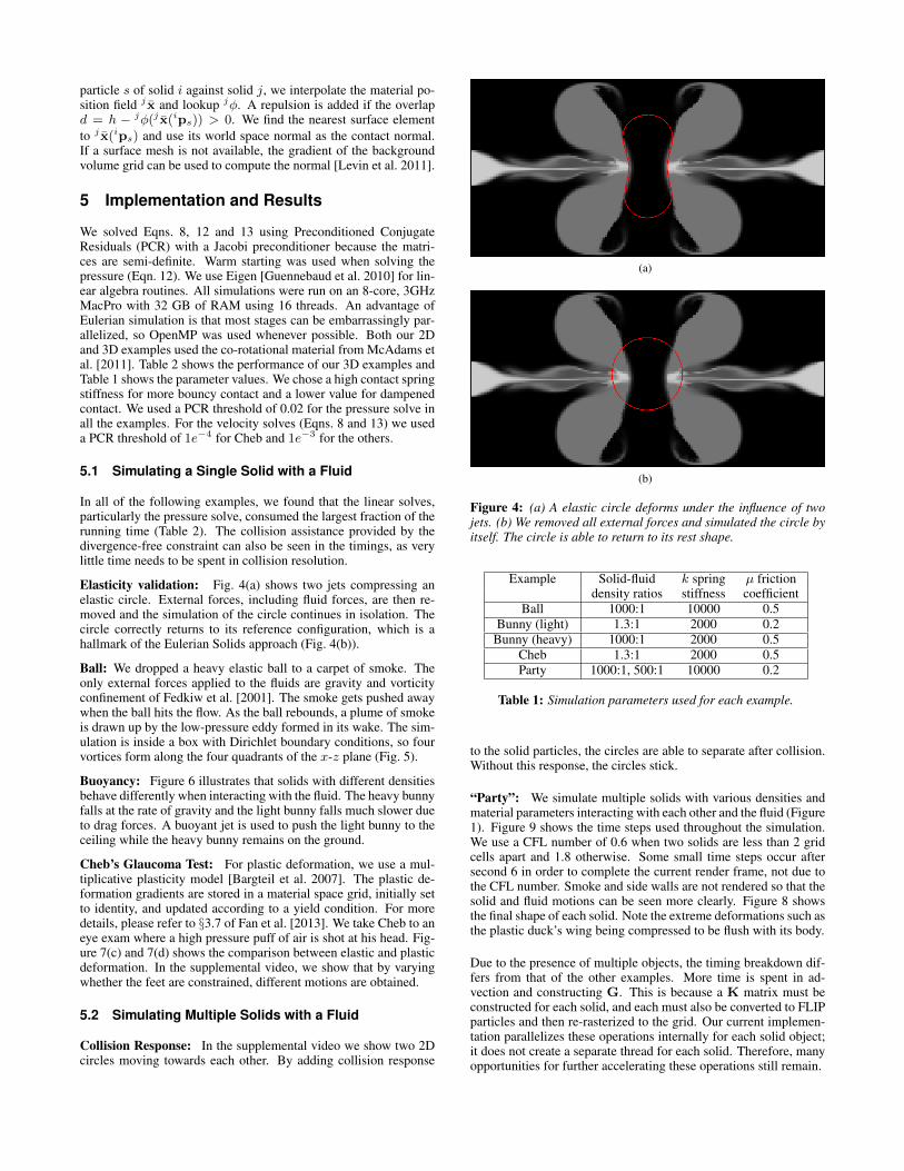
Elasticity validation: Fig. 4(a) shows two jets compressing anelastic circle. External forces, including fluid forces, are then re-moved and the simulation of the circle continues in isolation. Thecircle correctly returns to its reference configuration, which is ahallmark of the Eulerian Solids approach (Fig. 4(b)).

Ball: We dropped a heavy elastic ball to a carpet of smoke. Theonly external forces applied to the fluids are gravity and vorticityconfinement of Fedkiw et al. [2001]. The smoke gets pushed awaywhen the ball hits the flow. As the ball rebounds, a plume of smokeis drawn up by the low-pressure eddy formed in its wake. The sim-ulation is inside a box with Dirichlet boundary conditions, so fourvortices form along the four quadrants of the x-z plane (Fig. 5).

Buoyancy: Figure 6 illustrates that solids with different densitiesbehave differently when interacting with the fluid. The heavy bunnyfalls at the rate of gravity and the light bunny falls much slower dueto drag forces. A buoyant jet is used to push the light bunny to theceiling while the heavy bunny remains on the ground.

Cheb’s Glaucoma Test: For plastic deformation, we use a mul-tiplicative plasticity model [Bargteil et al. 2007]. The plastic de-formation gradients are stored in a material space grid, initially setto identity, and updated according to a yield condition. For moredetails, please refer to §3.7 of Fan et al. [2013]. We take Cheb to aneye exam where a high pressure puff of air is shot at his head. Fig-ure 7(c) and 7(d) shows the comparison between elastic and plasticdeformation. In the supplemental video, we show that by varyingwhether the feet are constrained, different motions are obtained.

5.2 Simulating Multiple Solids with a Fluid

Collision Response: In the supplemental video we show two 2Dcircles moving towards each other. By adding collision response

(a)

(b)

Figure 4: (a) A elastic circle deforms under the influence of twojets. (b) We removed all external forces and simulated the circle byitself. The circle is able to return to its rest shape.

Example Solid-fluid k spring µ frictiondensity ratios stiffness coefficient

Ball 1000:1 10000 0.5Bunny (light) 1.3:1 2000 0.2

Bunny (heavy) 1000:1 2000 0.5Cheb 1.3:1 2000 0.5Party 1000:1, 500:1 10000 0.2

Table 1: Simulation parameters used for each example.

to the solid particles, the circles are able to separate after collision.Without this response, the circles stick.

“Party”: We simulate multiple solids with various densities andmaterial parameters interacting with each other and the fluid (Figure1). Figure 9 shows the time steps used throughout the simulation.We use a CFL number of 0.6 when two solids are less than 2 gridcells apart and 1.8 otherwise. Some small time steps occur aftersecond 6 in order to complete the current render frame, not due tothe CFL number. Smoke and side walls are not rendered so that thesolid and fluid motions can be seen more clearly. Figure 8 showsthe final shape of each solid. Note the extreme deformations such asthe plastic duck’s wing being compressed to be flush with its body.

Due to the presence of multiple objects, the timing breakdown dif-fers from that of the other examples. More time is spent in ad-vection and constructing G. This is because a K matrix must beconstructed for each solid, and each must also be converted to FLIPparticles and then re-rasterized to the grid. Our current implemen-tation parallelizes these operations internally for each solid object;it does not create a separate thread for each solid. Therefore, manyopportunities for further accelerating these operations still remain.

Example Grid Dimensions Avg. Min. Avg. Compute Velocity solves Pressure Advection Collisiontimestep timestep time/frame G (line 8) (lines 9, 11) solve (line 10) (lines 13, 18) (line 14)

Ball 120 × 140 × 120 0.025 0.0016 6.54s 0.84s 0.12s 2.83s 1.12s 0.01sLight Bunny 144 × 200 × 144 0.0369 0.0064 17.4s 1.32s 5.02s 6.21s 1.72s 0.016sHeavy Bunny 144 × 200 × 144 0.0236 0.00058 16.9s 1.35s 2.47s 8.31s 1.68s 0.016s

Cheb 120 × 100 × 80 0.021 0.0023 6.97s 1.55s 1.10s 1.10s 1.37s 0.01sParty 200 × 180 × 200 0.0133 0.00083 54.1s 13.6s 6.72s 12.1s 14.46s 0.25s

Table 2: For each example, the size of the spatial grid, average / minimum simulation time step sizes and average per-frame simulation timesare reported. We also list the computation times of key stages of Algorithm 1. All timings are reported in seconds.

Figure 5: A plume rises as an elastically deforming ball bouncesup from a smoky floor.

Figure 6: Different solid densities behave differently under buoyantflow. When the solid-fluid density ratio is 1.3:1 (left), the smokeplumes causes the bunny to rise like a balloon. When the ratio is1000:1 (right), the bunny drops like a rock.

6 Discussion and Future WorkIn this paper we have shown how to simulate a two-way couplingbetween solids and a fluid where the underlying representation isentirely Eulerian. This allows us to generate simulations that fea-ture large deformations and frictional contact, all the while captur-ing visually interesting fluid effects. We believe our method pro-duces examples that are more complex than previous approachesand avoids the complexities of Lagrangian, mesh-based simulation.

Our method has several limitations, the most obvious of which isthat the fluid is limited to a single phase. Extending this approach tohigh-quality, fully Eulerian liquid simulations [Heo and Ko 2010] isa direction for future work. As the technique is Eulerian, handlingfeatures that are smaller than a single grid cell, e.g. rods and thinshells [Guendelman et al. 2005], remains a challenge. This samedifficulty extends to fracture patterns, though extended finite ele-ment approaches [Kaufmann et al. 2009] offer a potential solution.

(a) (b)

(c) (d)

Figure 7: (a) Cheb has a high pressure puff of air shot at his head.(b) Same frame, viewed from the front, with smoke removed to makethe deformation more visible. (c) Final frame, elastic deformation.(d) Final frame, plastic deformation. Note that the dent in his headpersists, as well as the deformations to his ears.

Furthermore, while we have shown that an implicit integrationscheme can be effective when simulating this coupling problem,other schemes that enable even larger timesteps [Lentine et al.2012], or preserve more structure given the same timestep [Mullenet al. 2009], would be welcome additions to this work. Finally, it re-mains to be seen whether a combination of Eulerian-on-Lagrangian[Fan et al. 2013] and subspace methods [Kim and Delaney 2013;Liu et al. 2015] could be used to accelerate the overall simulation.

Acknowledgements

This work was supported by a National Science Foundation CA-REER award (IIS-1253948). Any opinions, findings, and conclu-sions or recommendations expressed in this material are those of theauthors and do not necessarily reflect the views of the National Sci-ence Foundation. We acknowledge support from the Center for Sci-entific Computing from the CNSI, MRL: an NSF MRSEC (DMR-1121053) and Hewlett Packard.

Figure 8: The final shapes of party members. The duck and penguinon the left are plastic while the other three are elastic.

References

AKINCI, N., CORNELIS, J., AKINCI, G., AND TESCHNER, M.2013. Coupling elastic solids with smoothed particle hydrody-namics fluids. Comp. Anim. and Virtual Worlds, 195–203.

BAAIJENS, F. P. T. 2001. A fictitious domain mortar elementmethod for fluid/structure interaction. International Journal forNumerical Methods in Fluids 35, 7, 743–761.

BARGTEIL, A. W., WOJTAN, C., HODGINS, J. K., AND TURK,G. 2007. A finite element method for animating large viscoplas-tic flow. ACM Trans. Graph. 26, 3.

BATTY, C., BERTAILS, F., AND BRIDSON, R. 2007. A fast vari-ational framework for accurate solid-fluid coupling. In ACMTrans. Graph., vol. 26, ACM, 100.

BELYTSCHKO, T., LIU, W. K., MORAN, B., AND ELKHODARY,K. 2013. Nonlinear finite elements for continua and structures.John Wiley & Sons.

BOUAZIZ, S., MARTIN, S., LIU, T., KAVAN, L., AND PAULY, M.2014. Projective dynamics: Fusing constraint projections for fastsimulation. ACM Trans. Graph. 33, 4 (July), 154:1–154:11.

BRACKBILL, J., AND RUPPEL, H. 1986. Flip: A method foradaptively zoned, particle-in-cell calculations of fluid flows intwo dimensions. J. of Comp. Phys. 65, 2, 314–343.

BRIDSON, R., FEDKIW, R., AND ANDERSON, J. 2002. Robusttreatment of collisions, contact and friction for cloth animation.In ACM Trans. Graph., 594–603.

BRIDSON, R. 2008. Fluid Simulation for Computer Graphics. AKPeters.

CARLSON, M., MUCHA, P. J., AND TURK, G. 2004. Rigid fluid:Animating the interplay between rigid bodies and fluid. ACMTrans. Graph. 23, 3 (Aug.), 377–384.

CHENTANEZ, N., GOKTEKIN, T. G., FELDMAN, B. E., ANDO’BRIEN, J. F. 2006. Simultaneous coupling of fluids anddeformable bodies. In ACM SIGGRAPH/Eurographics Symp.Comp. Anim., 83–89.

CLAUSEN, P., WICKE, M., SHEWCHUK, J. R., AND O’BRIEN,J. F. 2013. Simulating liquids and solid-liquid interactions withlagrangian meshes. ACM Trans. Graph., 17:1–15.

FAN, Y., LITVEN, J., LEVIN, D. I., AND PAI, D. K. 2013.Eulerian-on-lagrangian simulation. ACM Trans. Graph..

FEDKIW, R., STAM, J., AND JENSEN, H. W. 2001. Visual simu-lation of smoke. In Proceedings of SIGGRAPH, 15–22.

GUENDELMAN, E., SELLE, A., LOSASSO, F., AND FEDKIW, R.2005. Coupling water and smoke to thin deformable and rigidshells. ACM Trans. Graph. 24, 3 (July), 973–981.

GUENNEBAUD, G., JACOB, B., ET AL., 2010. Eigen v3.http://eigen.tuxfamily.org.

HE, X., LIU, N., WANG, G., ZHANG, F., LI, S., SHAO, S., ANDWANG, H. 2012. Staggered meshless solid-fluid coupling. ACMTrans. Graph. 31, 6 (Nov.), 149:1–149:12.

HEO, N., AND KO, H.-S. 2010. Detail-preserving fully-eulerianinterface tracking framework. ACM Trans. Graph. 29, 6 (Dec.).

IHMSEN, M., ORTHMANN, J., SOLENTHALER, B., KOLB, A.,AND TESCHNER, M. 2014. SPH Fluids in Computer Graphics.In Eurographics State of the Art Reports.

IRVING, G., SCHROEDER, C., AND FEDKIW, R. 2007. Volumeconserving finite element simulations of deformable models. InACM Trans. Graph., vol. 26.

JIANG, C., SCHROEDER, C., SELLE, A., TERAN, J., AND STOM-AKHIN, A. 2015. The affine particle-in-cell method. ACM Trans.Graph. 34, 4 (July), 51:1–51:10.

JIANG, C., SCHROEDER, C., TERAN, J., STOMAKHIN, A., ANDSELLE, A. 2016. The material point method for simulatingcontinuum materials. In ACM SIGGRAPH Courses.

KAMRIN, K., RYCROFT, C. H., AND NAVE, J.-C. 2012. Ref-erence map technique for finite-strain elasticity and fluid–solidinteraction. Journal of the Mechanics and Physics of Solids 60,11 (Nov.), 1952–1969.

KAUFMANN, P., MARTIN, S., BOTSCH, M., GRINSPUN, E., ANDGROSS, M. 2009. Enrichment textures for detailed cutting ofshells. ACM Trans. Graph. 28, 3 (July), 50:1–50:10.

KIM, T., AND DELANEY, J. 2013. Subspace fluid re-simulation.ACM Trans. Graph. 32, 4 (July), 62:1–62:9.

KLINGNER, B. M., FELDMAN, B. E., CHENTANEZ, N., ANDO’BRIEN, J. F. 2006. Fluid animation with dynamic meshes.ACM Trans. Graph. 25, 3 (July), 820–825.

LENAERTS, T., ADAMS, B., AND DUTRE, P. 2008. Porous flow inparticle-based fluid simulations. In ACM Trans. Graph., vol. 27,49:1–49:8.

LENTINE, M., CONG, M., PATKAR, S., AND FEDKIW, R. 2012.Simulating free surface flow with very large time steps. In ACMSIGGRAPH/Eurographics Symp. Comp. Anim., 107–116.

LEVIN, D. I., LITVEN, J., JONES, G. L., SUEDA, S., AND PAI,D. K. 2011. Eulerian solid simulation with contact. In ACMTrans. Graph., vol. 30.

LIU, B., MASON, G., HODGSON, J., TONG, Y., AND DESBRUN,M. 2015. Model-reduced variational fluid simulation. ACMTrans. Graph. 34, 6 (Oct.), 244:1–244:12.

MACKLIN, M., AND MULLER, M. 2013. Position based fluids.ACM Trans. Graph. 32, 4, 104.

MACKLIN, M., MULLER, M., CHENTANEZ, N., AND KIM, T.-Y.2014. Unified particle physics for real-time applications. ACMTrans. Graph. 33, 4 (July), 153:1–153:12.

MCADAMS, A., SELLE, A., WARD, K., SIFAKIS, E., ANDTERAN, J. 2009. Detail preserving continuum simulation ofstraight hair. ACM Trans. Graph. 28, 3, 62:1–62:6.

MCADAMS, A., ZHU, Y., SELLE, A., EMPEY, M., TAMSTORF,R., TERAN, J., AND SIFAKIS, E. 2011. Efficient elasticityfor character skinning with contact and collisions. ACM Trans.Graph. 30, 4 (July), 37:1–37:12.

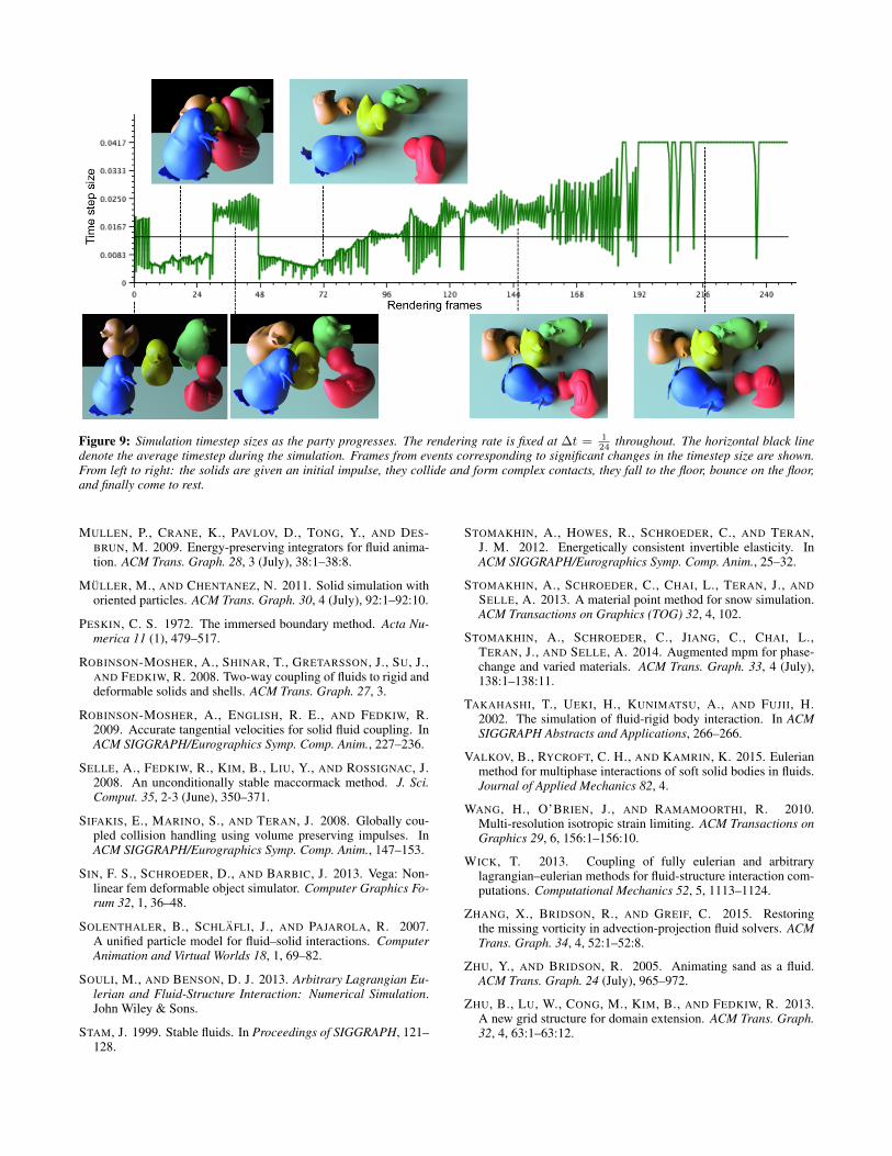
Figure 9: Simulation timestep sizes as the party progresses. The rendering rate is fixed at ∆t = 124

throughout. The horizontal black linedenote the average timestep during the simulation. Frames from events corresponding to significant changes in the timestep size are shown.From left to right: the solids are given an initial impulse, they collide and form complex contacts, they fall to the floor, bounce on the floor,and finally come to rest.

MULLEN, P., CRANE, K., PAVLOV, D., TONG, Y., AND DES-BRUN, M. 2009. Energy-preserving integrators for fluid anima-tion. ACM Trans. Graph. 28, 3 (July), 38:1–38:8.

MULLER, M., AND CHENTANEZ, N. 2011. Solid simulation withoriented particles. ACM Trans. Graph. 30, 4 (July), 92:1–92:10.

PESKIN, C. S. 1972. The immersed boundary method. Acta Nu-merica 11 (1), 479–517.

ROBINSON-MOSHER, A., SHINAR, T., GRETARSSON, J., SU, J.,AND FEDKIW, R. 2008. Two-way coupling of fluids to rigid anddeformable solids and shells. ACM Trans. Graph. 27, 3.

ROBINSON-MOSHER, A., ENGLISH, R. E., AND FEDKIW, R.2009. Accurate tangential velocities for solid fluid coupling. InACM SIGGRAPH/Eurographics Symp. Comp. Anim., 227–236.

SELLE, A., FEDKIW, R., KIM, B., LIU, Y., AND ROSSIGNAC, J.2008. An unconditionally stable maccormack method. J. Sci.Comput. 35, 2-3 (June), 350–371.

SIFAKIS, E., MARINO, S., AND TERAN, J. 2008. Globally cou-pled collision handling using volume preserving impulses. InACM SIGGRAPH/Eurographics Symp. Comp. Anim., 147–153.

SIN, F. S., SCHROEDER, D., AND BARBIC, J. 2013. Vega: Non-linear fem deformable object simulator. Computer Graphics Fo-rum 32, 1, 36–48.

SOLENTHALER, B., SCHLAFLI, J., AND PAJAROLA, R. 2007.A unified particle model for fluid–solid interactions. ComputerAnimation and Virtual Worlds 18, 1, 69–82.

SOULI, M., AND BENSON, D. J. 2013. Arbitrary Lagrangian Eu-lerian and Fluid-Structure Interaction: Numerical Simulation.John Wiley & Sons.

STAM, J. 1999. Stable fluids. In Proceedings of SIGGRAPH, 121–128.

STOMAKHIN, A., HOWES, R., SCHROEDER, C., AND TERAN,J. M. 2012. Energetically consistent invertible elasticity. InACM SIGGRAPH/Eurographics Symp. Comp. Anim., 25–32.

STOMAKHIN, A., SCHROEDER, C., CHAI, L., TERAN, J., ANDSELLE, A. 2013. A material point method for snow simulation.ACM Transactions on Graphics (TOG) 32, 4, 102.

STOMAKHIN, A., SCHROEDER, C., JIANG, C., CHAI, L.,TERAN, J., AND SELLE, A. 2014. Augmented mpm for phase-change and varied materials. ACM Trans. Graph. 33, 4 (July),138:1–138:11.

TAKAHASHI, T., UEKI, H., KUNIMATSU, A., AND FUJII, H.2002. The simulation of fluid-rigid body interaction. In ACMSIGGRAPH Abstracts and Applications, 266–266.

VALKOV, B., RYCROFT, C. H., AND KAMRIN, K. 2015. Eulerianmethod for multiphase interactions of soft solid bodies in fluids.Journal of Applied Mechanics 82, 4.

WANG, H., O’BRIEN, J., AND RAMAMOORTHI, R. 2010.Multi-resolution isotropic strain limiting. ACM Transactions onGraphics 29, 6, 156:1–156:10.

WICK, T. 2013. Coupling of fully eulerian and arbitrarylagrangian–eulerian methods for fluid-structure interaction com-putations. Computational Mechanics 52, 5, 1113–1124.

ZHANG, X., BRIDSON, R., AND GREIF, C. 2015. Restoringthe missing vorticity in advection-projection fluid solvers. ACMTrans. Graph. 34, 4, 52:1–52:8.

ZHU, Y., AND BRIDSON, R. 2005. Animating sand as a fluid.ACM Trans. Graph. 24 (July), 965–972.

ZHU, B., LU, W., CONG, M., KIM, B., AND FEDKIW, R. 2013.A new grid structure for domain extension. ACM Trans. Graph.32, 4, 63:1–63:12.