
Eulerian Hydrodynamic Code Computing Muhicomponent Reactive
42
I LA-;846 C38 CIC-14 REPORT COLLECTION REPRODUCTION ct2Py 2DE: A Two-Dimensional Continuous Eulerian Hydrodynamic Code for Computing Muhicomponent Reactive Hydrodynamic Problems d : 10s scientific laboratory of the university of California } alamos L LOS ALAMOS, NEW MEXICO 87544 4\. UNITED STATES ATOMIC ENERGY COMMISSION CONTRACT W-7405-ENG. 36
Transcript of Eulerian Hydrodynamic Code Computing Muhicomponent Reactive

ILA-;846
C38
CIC-14 REPORT COLLECTION
REPRODUCTIONct2Py
2DE: A Two-Dimensional Continuous
Eulerian Hydrodynamic Code for
Computing Muhicomponent
Reactive Hydrodynamic Problems
d:10sscientific laboratory
of the university of California
} alamos
LLOS ALAMOS, NEW MEXICO 87544
4\.
UNITED STATES
ATOMIC ENERGY COMMISSION
CONTRACT W-7405-ENG. 36

This report was prepared as an account of work sponsored by the United
States Government. Neither the United States nor the United States AtomicEnergy Commission, nor any of their employees, nor any of their contrac-
tors, sukontractors, or their employees, makes any warranty, express or im-plied, or assumes any legal liability or responsibility for the accuracy, com-pleteness or usefulness of any information, apparatus, product or process dis-closed, or represents that its use would not infringe privately owned rights.
Printed in the United States of America. Available fromNational Technical Information Service
U. S. Department of Commerce5285 Port Royal Road
Springfield, Virginia 22151Price: Printed Copy $3.00; Microfiche $0.95

10
LA-4846UC-32
ISSUED: March 1972
Icimosscientific laboratory
of the university of CaliforniaLOS ALAMOS. NEW MEXICO 87544
/ “\
2DE: A Two-Dimensional Continuous
Eulerian Hydrodynamic Code for
Computing Muhicomponentr Reactive Hydrodynamic Problems
by
James D. KershnerCharles L. Mader
This report supersedes LA-3629-MS.
ABOUT THIS REPORT
This official electronic version was created by scanning the best available paper or microfiche copy of the original report at a 300 dpi resolution. Original color illustrations appear as black and white images. For additional information or comments, contact: Library Without Walls Project Los Alamos National Laboratory Research Library Los Alamos, NM 87544 Phone: (505)667-4448 E-mail: [email protected]

2DE: A TWO-DIMENSIONAL
CONTINUOUS EULERIA,N HYDRODYNAMIC
CODE FOR COMPUTING MULTICOMPONENT
REACTIVE HYDRODYNAMIC PROBLEMS
by
James D. Kershner and Charles L. Mader
ABSTRACT
This report describes a code called 2DE that computes two-dimensionalreactive multicomponent hydrodyn~ic problems in slab or cylindrical geome -try using continuous Eulerian equations of motion.
Realistic equation-of-state treatments for mixed cells are combined withthe donor-acceptor-cell method to calculate mixed cell fluxes.
The calculated results using the 2DE code are compared with Lagrangiancalculations for several one - and two-dime nsional problems.
1. INTRODUCTION
The finite difference analogs of the Eulerian
equations of motion have been studied at the Los
Alamos Scientific Laboratory (LASL) for’ more
than ten years. The initial work of Richl was fol-2
lowed by that of Gentry, Martin, and Daly, which
resulted in the FLIC method. A one -component
Eulerian hydrodynamic code written by Gage and
Mader3 in STRETCH machine language used the
features of the FLIC method and the OIL method4
developed at General Atomic Division of General
Dynamics Corporation. The 2DE code was used
to solve reactive hydrodynamic problems that re -
quired high resolution of highly distorted flows.
Results of the detonation physics studies using
the code are described in Refs. 5 through 9.
The study described in this report was under-
taken to determine whether or not the continuous
Eu.lerian approach to reactive hydrodynamic
problems, where severe distortions prevent solu-
tion by Lagrangian methods, could be extended to
multicomponent problems in reactive hydrodynam-
ics. Also, because of the untimely death of
STRETCH, a FORTRAN version of the one-compo-
nent Eulerian code was needed.
Multic omponent Eulerian calculations require
equations of state for mixed cells and methods for
moving mass and its associated state values into
and out of mixed cells. The particle-in-cell (PIG)
method uses particles for this movement. We
previously had developed realistic equation-of-
state treatments for mixed cells using the PIG
method described in Ref. 10. We have extended
the mixed equation-of-state treatxnents to include
several cases not considered previously and have
used the donor-acceptor method for moving mass
and its ass ociated state values as determined by
the mixed equations of state.
1

The donor-acceptor method developed by John-
son” has been used by several investigators to
solve a variety of problems. The donor-acceptor
method for determining the mass flux was chosen
wer other methods, such as those proposed by
Hirt1213and developed by Hageman and Walsh,
only because of its ease of application. Ideally,
several methods for mass flux calculations should
be available in a general-purpose Eulerian code so
that the best method for a particular problem can
be used.,
Because reactive hydrodynamic problems re-
quire as much numerical resolution as possible,
the 2DE code (named after its STRETCH father) was
written to make maximum use of the Iarge capacity
memory devices on the CDC 7600 data processing
sys tern.
This report describes the method in complete
detail. It ah o presents sufficient details to enable
the reader to follow and modify the code. The latter
information is not of interest to the casual reader;
therefore, the more tedious descriptions of the mix-
ture equation-of -state treatments and derivations
of the various equations are described in Appendix-
es A, B, and C.
II. THE HYDRODYNAMIC EQUATIONS
The partial differential equations for non-
viscous, nonconducting, compressible fluid flow
in cylindrical coordinates are
(*+@&+ @=-P&#
(
~+uaup at )
~+vg =-g
(
fl+ug+vg
).-$
P at
and
u‘K )
Mass,
Momentum,
The equations, written in finite-difference form
appropriate to a fixed (Eulerian) mesh, are used
to determine the dynamics of the fluid. The fluid
is moved by a continuous mass transport method.
The fir st of the above equations, that of mass
conservation, is automatically satisfied. The mo-
mentum and energy equations are treated as fol-
lows . k the first step, contributions to the time
derivatives which arise from the terms involving
pressure are calculated. Mass is not moved at
this step; thus, the transport terms are dropped.
Tentative new values of velocity and internal ener-
gy are calculated for each cell.
In the second step, the mass is moved accord-
ing to the ceLl velocity. The mass crosuing cell
boundaries carries with it into the new cells appro-
priate fractions of the mass, momentum, and ener-
gy of the cells from which it came. This second
step accomplishes the transport that was neglected
in the first step.
In the third step, the amount of chemical reac-
tion is determined, and the new cell pressure is
computed using the HOM equations of state.
The equations we shall difference are of the
form
au iwfil,p~=- aR
and
2

III. THE C.ODLNG EQUATIONS AND TECHNIQUES Cell quantities:
P - CM - Cell density
Problem Boundaries I - CI - Cell interml energy
Axis
Continuum
EP - CP - Cell pressure
T - CT - Cell temperature
W - CW1 - Cell mass fraction for unburnedexplosive
Continuum U-cu - Cell r or x velocity
v-cv - Cell z velocity
; - RHOT - Tilde dens ity
q - Ql, Q2, Q3, Q4 - ViscositiesPiston (Constant Input)
Boundarv c- CUB - Cell R velocity tilde
Cell Sides
3
2❑ 4
1
The Initial Problem SetuD
or Continuum ~- CVB - Cell Z velocity tilde
AM - DMASS - Density increment for massmovement
LIE-DE - Energy increment
AW-DW - M.ass fraction increment
APU - DPU - Momentum in R direction increment
APV - DPV - Momentum in Z direction increment
ID - CID - Cell identification word
The cell ID word contains a material identifier,
mixed cell pointers, flags for span, tensio~
and mate rial type. It also carries temporary
flags which are set when DE or DW is calculated
by the mixed cell routine.
A Phase I. Equation of State and Reaction
The pressure and temperature are calculated
from the density, internal energy, and cell mass
fractions using the subroutines HOM, HOM2S,
HOMSG, HOM 2G, or HOM2SG described in Appen-
dix A. Mtied cells carry the individual compo-
nent densities and energies as calculated from
mixture equation of state.
Lf AV’/V’ (V’= ‘), and AI/1, from the neigh-P
boring cell and the present cell are less than
1234 5=1
Ror X
—U Velocity
O. 0005, the previous cell P and
Pij=P. and Ti, j = T., l-l, j l-l, j”
Knowing T, we calculate .W
henius rate law
-E*/R T~w=-z we g ,
T are used, i. e.,
using the Arr -
where Z is the frequency factor, E* is the
activation energy, Rg is the gas constant, and
3

6t is the time increment. In difference form this
is
~n+ 1 . ~n- tit Z Wne
-E*/RgTn+l.
1, If cell temperature is less than MINWT
(1000), reaction is not permitted.
2. If CW1 is less than GASW (O. 02), set
Cwl. o.
3. Do not react for first VCNT ( 25) cycles.
4. If CT is less than TO, CT = TO and if CP
is less than PO and tension flag is O, set CP = PO.
Phases I and II are skipped if ~~ ~< MING RHO
+ (p. - MTNGRH~ (W; j). This is for handling free
surfaces to eliminate false diffusion. MINGRHO =
O. 5. For gases at free surfaces ~j is replaced
by one.
B. Phase II. Viscosity and Velocity
1. Viscosity Equations3
u2 GRID 4
1
c21. .=qn.1, J l, J- *
= C23.I, j-1
except on boundary 1 when Qli ~ . 0.0,
or on piston boundary when
Q1 . =K(p:j + MAPP) (VA.PP - < ~)1, 1 ,
if VAPP > Vn1, 1
=0.0 if VAPP < V?1,1 .
Q2. . = q?~SJ l-~ j
= Q4.I-l, j
except on axis boundary 2 when
Q2l,j = 2Q\, j- “2,j .
Q3n
i,j=$, j~ = K ‘~, j + Pi, j+l )(v; j- fl, j+l)
n nif V. 2 V.
1, j 1, ji-1
=0.0 ifv?j<v?# 1, j+ I
except Q3. = O. 0 on continuativeI,JMAX
boundary 3.
Q4. . = q?l+& j
= K (P; j + ;+l, j) (U:j - U;+l, j)b J
ifu? >UnlJj i+l, j
=0.0 ifun <u?1, j 1+1, j
except on c ontinuative boundary 4 when
Q4IMAX, j
=0.0
2. Velocity Equations
P1 = Pnl, j-1
except on piston boundary 1, P1 = PAPP
or on continuative boundary 1, P 1 = Pn1,1.
P2 = P?l-l, j
except on axis boundary 2, P2 . PnI,j “
P3 = Pn1, j+l
except on continuative boundary 3,
P3 = P: JM= .,
P4 = PnI.i-l, j
except on continuative boundary 4,
P4 = P?1, IMAX .
Q2, P2
Q3, P3
Cl
P.n .1SJ. P4, Q4ipj
P1
Q1

‘n & (1(i-l) (P4-P2) + P4-P~ ju .U; j-—— - ,
ipj 2i-1P~j~ I
+ (24.)
-Q2ij.L j s
3. Internal Energy Calculation
For ~~ i < MINGRHO + (p. - MINGRHO)(W~, j) ~—7 .
E:, j = I;, j and the rest of Phase III is skipped.
U1 = (Un +;? .) .l-l, j I-l, J
.= V?.- ~bt ( ) ‘2 = (“~+l,j + ‘i+l, j)”-nv.
12J % J G~ -1-Q3. - Q1.
Pi, j b j hj “
V1 = (Vn + 7 ).I, j-1 qj-1
whereV2= (Vn +.7 )0
1, j-l-l 1, j+li=l ,2, . . . .. IMAX
T3 = (~, j +;~j).“=1, 2,....,J NJMAX~*JMAX (for NJMAX
core increments containing JMAX rows Tl = (V~j +?~j).
each).
P4-P2Ln slab geometry, the qu~tity in { ] . —Exceptions:
2
Axis boundary, UI = 2(~ j + fi~ j) - U2P 9
C. Phase III. Internal Energy and fi Calculation Continuative boundary 4,
1. ~ Calculation U2 = (UnIU, j
+ GnIMAX, j)
Exceptions:
Piston boundary, V. . = VAPPI, J-l
Axis boundary, U. .= - u.l-~J 1+1, j
+ .2U. .1. J
boundary 3, V. . = v.I,J+l b j
boundary 4, U. = u.1+1, j h j
2. Piston Energy Constraints
For the first VCNT cycles,
Piston boundary, VI = 2VAPP
Continuative boundary 1, V1 = (V: ~ + ~i, ~)
Continuative boundary 3,
1+U2+2T3+U12i-1 o
Q4. .
[+ &’J ‘2-T3 +{= }1
Q2i j
[ { }]2U 1-- uI-T 3-
@ m
7?. =
[“l/2 (P; j + Q3i j) (V: - l/P;, j) + KE.
1, J b j+&
[P: j (V2 - VI) + Q3i j (V2 - Tl)
, ,
if V; 21/p? .ISJ 1)+Qli j (Tl - Vl) .
,
J?In slab geometry the quantities in { } are set
ifV~< l/p?. ,i, j 1, J
(
2 2
)
equal to zero.
where KE. .= 1/2 Gn. +vn1, J 1>J hj “
5
4. Total Ener gy Calculation
En .=?n% J [ 1i,ji-1/2 (V;j)z+(ti:j)z .
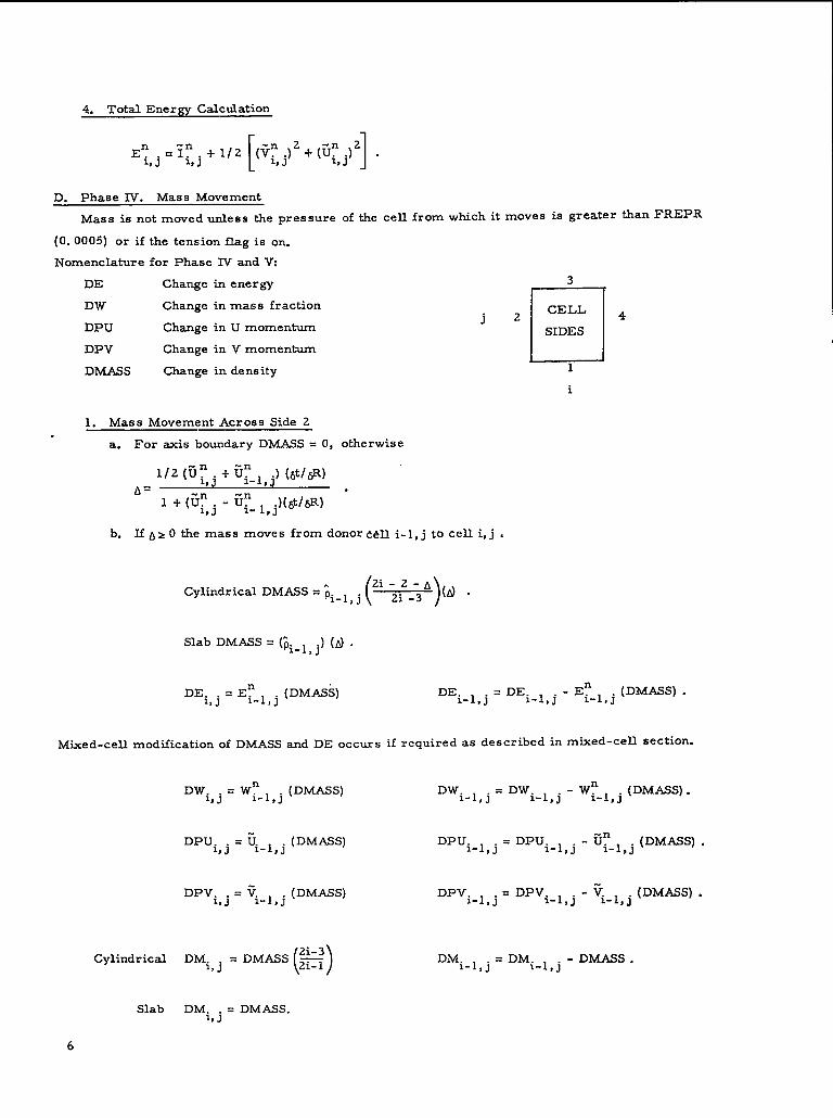
D. Phase IV. Mass Movement
Mass is not moved unless the pres sure of the cell from which it moves is greater than FREPR
(O. 0005) or if the tension flag is on.
Nomenclature for Phase lV and W
DE Change in energy
DW Change in mass fraction
DPU Change in U momentum
DPV Change in V momentum
DMASS Change in density
3
n
CELL ~j2
SIDES
1
i
1. Mass Movement Acress Side 2
a. For axis boundary DMASS . 0, otherwise
b. If A> O the mass moves from donor dell i-l, j to cell i, j ,
Slab DMASS = (hi-l, j) (A) .
DE. . = En1, J
,-1, j (DMAS5) DE. . = DE. ,-1, j (DMASS) .- En1-l, J I-ljj
Mixed-cell modification of DMASS and DE occurs if required as described in mixed-cell section.
DW. ,-1, j (DMASS).=W?1>J
(-)2i-3Cylindrical DM. = DMASS z~
h j
DW . . = DW. ~-l,j (DMASS) .- w?I-l, J z-l, j
DPU. . = DPU. i-l,j (DMASS) .- tin1-l, J z-l, j
DPV. . = DPV i-l, j (DMASS) .-v1-l, J i-l, j
DM. . = DM. - DMASS .l-l, J l-l, j
Slab DM. . = DMASS.Is J

c, If A C O, the mass moves from the donor cell i, j to acceptor cell i-l, j.
Cylindrical DMASS =$: j(2i -2-A)
(2i - 1)A, slab DMASS=~~j A.
,, j (DMASS)DE. . = E?1>J
Mixed-cell modification of DMASS and DE
Dwi, j = w:, j (DMAS.S)
DPU. . = ti;, j (DMASS)1, J
, j (DMASS)DPV. . = ;?l~J ,
DM . . = DMASS1, J
DE. . = DE. i, j (DMXS) .- En1-l, J l-l, j
occurs if required,
DW . .=DWi ~,j - ~, j (DM.MS).1-l, J
DPU. . = DPU. - fii, j (DMASS) .I-l, J z-l, j
DPV . . = DPV. - Vi, j (DMASS) .1-l, J l-l, j
(-)2i- 1Cylindrical DM. . = DM. - DMASS ~ .
1-l, J I-ljj
Slab DM. = DMASS .I-l$j
2. Mass Movement Acress Side 1
a. For a piston boundary
(VA-PP+w ,) (f$i%)., J
A= 1/2 . .(;;, j - VAPP) (&/&) + 1
For A< O, DMASS = O.
For ~> O, DMASS . (MAPP) (~, and the mass moves from the piston to cell i, j.
DE. . = DE.~, j + DMASS (EAPP) .1>J
DW. . = DW. , + DMASS (WAPP) .I, J 1, J
DPVi, j = DPV. + DMASSb j
DPU. . = DPUi, j + DMASSI,J
DM. . = DM. + DMASS .1, J 1, j
VAPP) .
UAPP) .

b. For continuative boundary 1 cell,
DE. n DE1Sj
,, j (DMASS) .i,j+En
Mixed-cell modifications of DMASS and DE occurs if required.
,, j (DMASS) .DWi j = DW. + W*, b j
DPV. . = DPV ,, j (DMASS) .i,j+i.1, J
DPU. . = DPU. ,, j (DM.ASS) .~,j+fi.% J
otherwise
1/2 (~, j + i;j-l) (&/#)
A =1 +(;:j - in~,j-l) (6t/6z) “
c. Lf A >0, the mass moves from donor cell i, j-l to acceptor cell i, j.
DM../lSS = (~i; j-l) (~ .
,, j-l (DMASS)DE. . = DE. + En DE. = DE. i,j-l (DMASS) .- En1, J b j l, j-1 l, j-1
Mixed-cell modification of DMASS and DE occurs if required.
DW . . = DW. ,,j-l (DNL4SS) DWi, j-l = DWi, j-l -+ w?1>J Igj
DPVi, j = DPV. ,, j- ~ (DMASS)+ Vn DPV . . = DPV. .bj l, J-l I, J-l
DPU . . = DPU , j_l (DMASS)i,j+ti? DPU. . = DPU. .1, J , %J-l l, J-~
DM. . = DM. . + DMASS DM. =DM. . -1, J ISJ l, j-1 l, J-1
,,j-l (DMASS) ,w.
,,j-l (DMASS) .- v.
,,j-l (DMASS) .- G.
DMASS .

d. If ~ <0, the mass moves from donor cell i, j to acceptor ce~ i, j-1.
DE. .=DE .+En i, j (DMASS)1, J i, J
DE. = DE. i j (DMASS) .- Enl, j-1 hj-1 ,
Mixed-cell modification of DMASS and DE occurs if required.
DWi, j = DWi, j + W; j (DMASS) DW. ,, j (DMASS) e=DW. . -Wnl, j-1 I, J-l
DPV . . = DPV. + ~i, j (DMASS) DPV. = DPV.1$J
,, j (DMASS) .- ??h j l, j-1 l, j-1
Dpui, j = Dpu. + fii, j (DMMS) DPU. = DPU. ,, ~ (DMASS) .-E..h j qj-1 l, j-1
DM. . = DM. + DMASS DM. = DM.1, J h j
- DMASS .I,j-1 l, j-1
3. Mass Movement Across Side 3
Except on continuative boundary 3, this mass movement is taken care of by the mass movement
across side 1 of the cell directIy above.
On the boundary 3,
A = (v:, j) (@fjz) .
DE. .= DE. . - Ei, j (DMASS) .1, J 1>J
Mixed-cell modification of DMA.SS and DE occurs if required.
DW. .= DW. .-W.I* J
, j (DMASS) .l>J >
DPVi j = DPV. . - ;i j (DMASS) .I>J s
DPUi, j = DPUi, j - ti.,, j (DMASS) .
DM. . = DM. - DMASS .1, J 1Pj
9

4. Mass Movement Acress Side 4
Except on the continuative boundary 4, this
mass movement is taken care of by the mass move-
ment across side 2 of the cell on its right.
For i = lhf~
A=0.5(3 tin -inu j
i-l, j) (at/@) .
a. A z O mass moves out of ceU i, j,
Cylindrical DMASS = (bi, j) * .
b. AS O mass moves into ce~ i,j .
Cylindrical DMASS = (2i-& (d‘~i, j) (2i+l)
for either a. or b. Slab DMASS = (pi, j) (L!) .
DE. ,, j (DMASS) ..= DE. .-E?Is J 1, J
Mixed-cell modification of DMASS and DE occurs
if required.
DW. = DW.h j b j
- W?, j (DMASS) .
DPVi j = DPV. i, j (DMASS)-v* h j
DPU = DPU.h j
- fii, j (DMASS)i$ j
DM. . = DM. - DMASS .% J h j
5. Mixed Cells—
The composition of the mass to be moved
from the donor to the acceptor cell is determined
as follows. Materials common to both the donor
and acceptor cells are moved according to the
mass fractions of common materials in the accep-
tor cell. If the donor and acceptor cell have no
common materials, then mass is moved according
to the mass fractions of & donor cell. The mass
to be moved from the donor cell has the density
and energy determined for that component or com-
ponents by the mixture equation-of-state calcula-
tion in Phase I.
1. Therefore, the DMASS term is cor-
rected by dividing by cell ~ used in Phase IV and
replacing it with the ~ of the material being m~ed
from the donor cell (~).
kDMASS = DM.ASS — .
P
If the mass of the material in the donor
cell is less than the total mass to be moved, the
remainder of the mass moved has the remaining
donor-cell composition density and energy.
2. The DE term is calculated using the
internal energy of the component being moved from
the donor cell as calculated from the mixture equa-
tion-of-state routines in Phase I.
n+ 1 n‘E DONOR = ‘E DONOR
- (DM.&SS) (Donor
Component I + Donor K. E. ) .
DEn+ 1ACCEPTOR
= DEnACCEPTOR
+ (DMASS) (Donor
Component I + Donor K. E. ) .
The mass fraction of decomposing explosive be-
tween a mixed and unmixed cell is treated as
follows . If the donor cell is mixed and explosive
is being moved to an acceptor cell, the donor cell
CW is not changed. If the acceptor cell is mixed
and explosive is being moved into the acceptor
cell the acceptor cell W is calculated by
n+ 1CWACCEPTOR=
b“’’’”’)(‘i!%%.}@f+%mNoR‘iCCEPTOR
+ DMASS
EXPLOSIVE
By convention CW is set to equal 1.0 for an inert
or O. 0 for a gas if the donor or acceptor does not
contain an explosive.
10

E. Phase V. Repartition
Add on mass moved quantities.
For p; j s MINGRHO + (Po-MINGRHO) (W; j) ,9
n+ 1P. “=P~, j+ DMi, j”1, J
w;+;=+ ‘p~j W;, j + DWi, j).
P. .1, J
V;:l =* ‘i~jp~j ‘Dpvi,j) “P.-L,J
n+ 1u.. =
ISJ& (fi; jp?j+DPUi j).
9P. .
,ISJ
For p; j s IvfIIVGRHO + (PO - MINGRHO) (Wn .),1, J
n-l-lP. .= P:, j + DM.
l,J hj “
wn+lL j
= ‘n+ (P;, j ,W;j+DW. .).l,J
Pi, j
un+ 1
=% (U; jp; j+ DPUi j).i] j > ,
‘i j
IY; =o. o..
IV. TEST PROBLEMS
The 2DE code has been used to calculate one-
component, two-d irnensional problems of a shock
in nitromethane inte ratting with a rectangular or
a cylindrical void. The results agreed with those
published in Ref. 6.
The 2DE code has been used to calculate the
one-dimensional, multi component problem of an
85 kbar shock in O. 04 cm of nitromethane des-
cribed by 100 cells in the Z direction, interacting
with a O. 016-cm slab of aluminum described by 40
cells, which had as its other interface O. 016 cm of
air at 1 atm initial pressure described by 40 cells.
The equation of state for nitromethane and alumi -
num were identical to those described in Ref. 10.
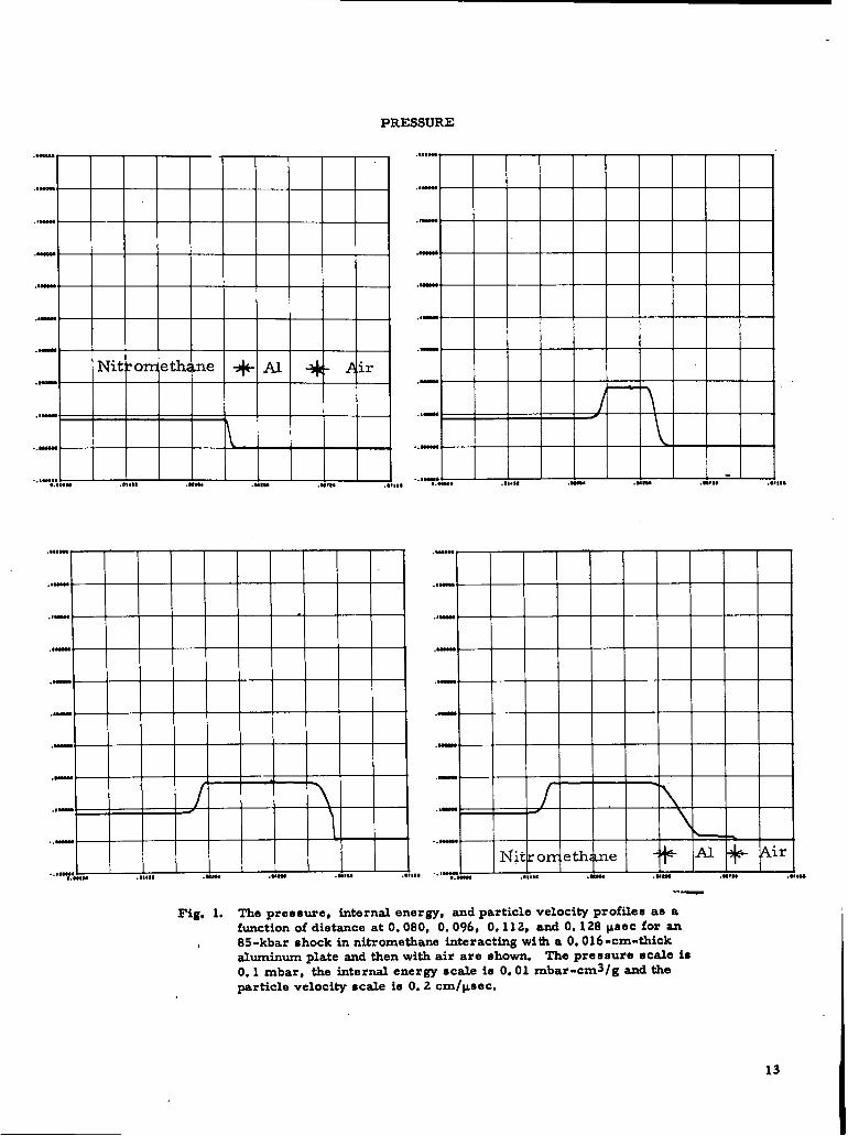
The calculated pressure, energy, and particle
velocity profiles are shown in Fig. 1. The re-
sults were compared with SIN14 one-dimensional
Lagrangian calculations for the same problem. A
comparison of the average results of the calc~a -
tions is shown below. The units are mbar, cm3/ g,3
mbar-cm /g, degrees Kelvin, and cm/@ec respec-
tively for pressure, specific volume, energy,,,
temperature and particle velocity.
Nitr ome thaneShock
PressureSpecific VolumeEnergyTemperatureParticle Velocity
Reflected Shock(Nitromethane)
PressureSpecific VolumeEnergyTemperatureParticle Velocity
Aluminum ShockPressureSpecific VolumeEnergyTemperatureParticle Velocity
Aluminum Rare-faction
PressureSpecific VolumeEnergyTemperatureParticle Velocity
Eulerian
O. 08580.54550.01461146.20.171
0.1780.46860.022481365.50.0967
0.17850.30710.0047487.10.0964
0.0080.35610.0007384.00.1873
Lagrangian
O. 08570.54550.01461181.90.171
0.17870.48580.02251436.10.0964
0.17860.30700.0046518.30.0964
0.00040.36030.0005355.50.1932
The agreement between the Lagranglan and
Eulerian calculations is adequate except at the ni-
trometham -alurninurn interface. In the Eulerian
calculation, the internal energy is 1170 too high in
the nitromethane cell next to the interface and is
11

10~0 too low in the aluminum cell next to the inter-
face. Such an error is in the expected direction
because the reflected shock Hugoniot has less ener-
gy than the single shock Hugoniots used to partition
the energy between the doubly shocked nitrome -
thane and the singly shocked aluminum in the mix-
ture equation- of-state routines. This suggests that
an improved mixture equation-of-state treat.ment
could be accomplished by keeping track of whether
the component had been previously shocked and by
partitioning the energy accordingly.
Of course, it is not correct to assume that the
Lagrangian calculation treated the boundary in an
exact manner. Because of the large density differ-
ence, the Lagrangian calculation had nitromethane
energies that were 6. 6y0 too high at the interface
and &uminum energies that were 2. 4% too low.
The 2DE code has been used to calculate the
two-dimensional, mu.tticomponent problem of an
85-kbar shock in a cylinder of nitrometha.ne inter-
acting with a O. 025-cm radius aluminum sphere
and an 85-kbar sho’qk in a slab of nitromethane in-
teracting with an aluininum rod. The calculation
was performed with 100 cells in the Z direction and
50 cells in the R direction of O. 001 cm. The re-
sults compared well with those obtained previously10
using the PIC technique in the EIC code which
were compared with PHERMEX radiographs of the
interaction of shocks in water with aluminum rods
(Ref. 15).
The is oplots for the aluminum rod being shock-
ed in nitromethane are shown at various times in
Fig. 2.
The results of these and other test problems
support our conclusion that the continuous Eule rian
approach to reactive hydrodynamic problems can be
use d to solve mul.tic omponent problems involving
r e active flow. Further improvement is possible in
the treatment of the mixture equations of state.
The mass flux treatment from mixed cells could be
improved by including more constraints on the do-
nor-acceptor method, and by including some
interface following technique such as those used
by Hageman and Walshl 3 and proposed by Hirt. 12
We plan to use the code in its present form to
study several reactive and nonreactive flow prob-
lems of current interest. We ah o plan to include
into the code the capability to describe elastic-
plastic and viscous flow similar to that used in
our two-dimensional reactive Lagrangian code
2DL. We plan to include other methods for de-
scribig the decomposition of the explosive such as
C-J volume burn, sharp-shock burn, heterogene-
ous sharp-shock partial reaction burn and Dremin
burn.
It is already apparent that a three-dimension-
al version of the 2DE code would be a useful tool
and would probably be more useful than a three-
dimensional particle Eulerian code such an the one
we studied in Ref. 16. Such a capability would
permit more realistic modeling of the reactive
fluid dynamics problems discussed in Refs. 6, 7,
and 9. It would, of course, be useful for studying
many other problems.
ACKNOWLEDGMENTS
We gratefully acknowledge the many helpful
discussions with R. Gentry, C. W. Hirt, and F.
H. Harlow of Group T-3; W. Orr, K, Meyer,
P. Blewett, C. Hamilton, and G. White of Group
TD-5; C. Forest of Group TD-6; K. Lathrop of
Group T-1; W. Goad of Gro~ T-DOT; J. Barnes
of Groy T-4; and W. Johnson and M. Walsh of
Systems, Science and Software.
12
PRESSURE
.,”,”
.,-
.,Onn
.-
.-
..-
.-
Nit rOlr.eth me + Al A ,ir.- .
.,-
..-
..,-,,.,.,C+” .0,.19 .W9U .“MO .mm. .,0,.,
.,.,9s9
..Non
.,Omn
Jcudf
.-
..-
.- ,
.-
.,- / “ 7..-...-,. .
Loon, .,,.,s .Mlu .Ut,i .96*1, .,,,,.
.,,,”.
..enu
.mnn
.4-
.-
.,.
..-
..,,,,,,,.,”” .,,,s, .0iu4 ,“no .M*” .,,,,,
..,,OM
..UNO
.,NNC
.—
.,OlOla
.-
.,-
..- ,
Ni tro meth z.ne
.‘%’.’lnn .0,.s, .- .“I,9 m*,,
Fig. L The preesure, internal energy, and particle velocity profiles as afunction of dietance at O. 080, 0.096, 0.1120 and O. 128 ~aec for an85 -kbar shock in nitromethane interacting with a O. 016 -cm-thickaluminum plate and then with air are shown. The pre Ecure oc~e iO0.1 mbar, the internal energy ecale is 0.01 mbar-cm3/g and the
,“
particle velocity scale is O. 2 cm/ksec.
13

XNTERN& ENERGY. . . ..
.“-
.-
“,
.,,-
.-
.-
.“-
.,-
.*,MN 1
,.nnd,.*.- .1,.s[ .MOn .64- .-ml .**,,,
.,,0”,
.“,.”
..,-
.
.-
.Un
.,141i9
.- f 4I
.,,-
. ..,”9N
.“NN
.“-
.,*9c0@
.-
.-
.“-
“-t+-!--l-kttH-j.,,9906
..,,COI
.“nn
.“-
.,mmo
.-
.“-
..-
.-
.,,-
Fig. 1. (Cent)
14

PARTICLE VELOCITY. . . . . . . .,.0- . ,._,,
..- .,-
.,- .*W
..- ..-
.- .--
..- ...-
---
Ni km- .Iet} .an.e + Al + -, \ir ‘“--..MIM ...oaw
..o- ---
-.,””, ...nm,
.,..-,,.0.,8U0 .,,.91 .C91M .Mw .,..00$.0-, .,,,18.Mtn, .,,,** .MIM .mm .S9M* .,.,,,
-.I,.,,.,,0
.●n.”
.mmm .
.. MOOa
.-
----
---
-..noa
---
...WSM
-,.,,,,,,,.,W .,,.s, .Mn4 “tu .“,,. .,.,.,
........ .
..nc+l
..-
..nnm
.-
...-
..-
Ni xo r.~e th are k- Al -+= Air----
..- I
----
.!.,-●.CO004 ..,.,, .Ouu .“8N .“,,, .●,,.’.
F’@. 1. (Cent)
15

1:-Y..6IR-- .1-- “ac ,,,Iv.mlu - Imnv*.,.-.,,
,?m?,.,.s.m,.lM- Cm4 Iu‘-em,” — Imznu. :.--01
ISOPYCNICS
r?!-Y,..”m .Icmx- C.cu 41,,-.-,,0 — Iwr..a. ,.-.0,
Fig. 2. The isopycnics, isobars, isotherms, isoenergy, and isovelocity in theX direction and isovelocity in Y direction profiles at O. 04, 0.08,0.13, and O. 18 psec for an 85-kbar shock in nitromethane interactingwith a O. 0Z5-cm-radius aluminum rod are shown. The contour inter-vals ● re O. 1 g/cm3, O. 01 mbar, 200° K, O. 005 mbar-cm3/g, andO. 01 cm/paec. The locations of the mixed cello are shown with an11*11’.
16

1 I,X-..” --- .,— “a ,,,
t mM9 - ,mm*ua ,.--”
Fig. 2. (Cent)
r:s.. ”ml “,-- car tat‘K,”, — Mmnti. ,.-.”
F-%%“...
R....../
I1 \ II ) J
;~~t..m=.ot.,cmmr- ,.(I, ,,,- :.....0 i----
17

I I;?2?7’”=.. .,-- “u ,,,
- Ima. 1.IC8R,U
ISOTHERM8
;&7m”=.. .,-- .= .,,-- ,mr . . . . r. NoR.#R
Fig. 20 (amt)
18

,%?4. ”E41 .I-- C.nl $0,-. — mm-a. I.--cl
rfi,i,,...m.. .,-- eel n,-. — Iw?tl... S.H-U
.%-,.,”-.,, .,-- c.lu .,,u-. — ,-.... s.-..
Hg. 2. (Cent)
19

ISOVELOCITY
4IN R DIRECTIO
,:.7C.”SIC...Klcu- C.ax N,..-. - Irr.s!u. l.nOR. m
r.-..-........%..,:2-*.IUHIM-- C.ax la“-ta. — mcwa. 1---- ,:X-,..”=.,, .,,-- Oat ,,,..rrL. — ,.ru... ,----
Fig. 2. (Cent)

r%’.. wr...,— C.ex ,,,v-m. - IuiDva. I. ICOR-U
rI
,:-7,. s.=.,,.,-- oat Ml.-m. — ,MIw.. ,.--m
I.SOVELOCITY
IN Z DIRECTION
,%Y.. ”OH .,— “ac to,.-m. — ,Muv.. s.--”
;~=x,.-.,, .,-- ,.M ,,,
- Imus.. ,.-. ”
fig. 2. (Cent)
21

APPENDIX A
EQUATIONS OF STATE
The HOM equation of state was used for a cell
containing a single comp one nt or any mixture of
condensed explosive and detonation products.
Temperature and pressure equilibrium was assum-
ed for any mixture of detonation products and con-
densed explosive in a cell.
When there are two components present in a
cell, separated by a boundary and not homogene-
ous ly mixed , it is reasonable to assume pressure
equilibrium, but the temperatures may be quite
cliff e r ent. For these systems we assumed that
the difference between the total Hugoniot energy
and the total cell energy was distributed between
the components according to the ratio of the Hu-
goniot energies of the components for two solids
or liquids, For two gases we assumed that the
difference between the total isentrope energy and
the total cell energy was distributed between the
components according to the ratio of the isen-
trope energies of the components. For a solid
and a gas we as surned that the difference between
the sum of the gas isentm~ energy and the solid
Hugoniot energy and the total cell energy was dis-
tributed behveen the components according to the
ratio of the gas isentm~ energy and the solid Hu-
goniot energy of the components.
When there are three components present in
a cell, an explosive, its detonation products, and
a third solid or liquid nonreactive component, the
equation of state is computed assuming tempera-
ture and pressure equilibrium for the detonat ion
products and condensed explosive, and pressure
equilibrium with the nonreactive component.
The equation-of -state subroutines require the
specific volume, internal energy, and mass frac-
tions of the components as input and iterate to give
the pressure, the individual densities, tempera-
tures, and energies of the components.
This treatment of the equation of state of
mixtures is attractive because if the state values
22
of the components are reasonably close to the
state value for the standard curve (the Hugoniot
for the solid or the isentrope for the gas), one can
have considerable confidence in the calculated re-
sults . For the gases it would be best to choose a
state value near those expected in the problem to
use for forming the isentr~pe.
Nomenclature:
c, s
cl, s]
‘v
c1v
I
P
SPA
SPALL P
T
USP
uP
us
v
V.
w
Xorx
Subscripts:
g
H
i
s
A
B
coefficients to a linear fit of Us
and UP
second set of coefficients to a
linear fit of Us and UP
heat capacity of condensed
component (cal/g/deg)
heat capacity of gaseous compo-
nent (cal/g/deg)
total internal energy (Mbar-
cm3/g)
pressure (Mbar)
spalling constant to relate span
pressure and tension rate
interface spalling pressure
temperature (°K)
ultimate spalling pressure
p article velocity
shock velocity
total volume (cm3/ g).
initial volume of condensed com-
ponent (cm3/ g)
mass fraction of undecomposed
explosive
mass fraction of solid or gaseous
component
gaseous component
Hugoniot
isentrope
condensed component
component A
c omp orient B

I. HOM
HOM is used for a single solid or gas compo-
nent and for mixtures of solid and gas components
in pressure and temperature equilibrmm.
The Method
A. Condensed Components
(The mass fraction, W, is 1; the internal ener-
gy, 1, is Is ;’ and the specific volume, V, is vs. )
For volumes less than Vo, the experimental Hu-
goniot data are expressed as a linear fit of the
shock and particle velocities. The Hugoniot tem-
peratures are computed using the Walsh and Chris-
tian technique.
u =C+ sups
C2(V - Vs)o‘H = .
PO - s(vo-v~)]2
in TH = Fs_ + GslnVs + Hs (lnVs)2 + Is(lnVs)3
4+ .Ts (lnVs) . (A-1)
>=+ PH(VO-VJ.
Ps = ~ (Is()
- IH) + PH, where ys . V ~s #v.”
(Is - IH) (23, 890)Ts=TH+
cv
(A- 2)
(A-3)
TWO sets of C and S coefficients may be given.
For Vs < MINV, the fit Us = Cl + S1 (Up) is used
with the corre spending changes to the above equa-
tions. Between MINV and VSW, the volume is set
equal to MINV, and U = Cl + S1 (Up) is used. Fors
volumes greater than V..
we use the Gruneiseno’equation of state and the P = O line as the standard
curve.
[
Cv v
( )1
YsP~= I-
s (3) (23890) (a) V: -1 ~ “
(Is) (23, 890)T=
s Cv+To .
The spilling option is not used if SPA <0.0001.
If Ps <USP, set P . SPALL P and set the spa.1.l .s
indicator. J-fp~ s SPA ~~(~lfi is the ten-
sion rate), and Ps ~SPMIN (5 x 10⁻³) set Ps =
SPALL P and set the span indicator. Do not span
if neither of the above conditions is satisfied.
B. Gas Components
(Mass Fraction, W, is O; the internal energy,
I, is Ig; and the specific volume, V, is V ~.) The
pressure, volume, temperature, and energy values
of the detonation products are computed using FOR-
TRAN BKW and are fitted by a method of least
squares to Eqs. (4) through (6). A gamma-law gas
may also be fit to these equations as a special case.
lnPi = A + BlnVg + C(lnVg)2 + D(lnVg)3 + E( lnVg)4.
(A-4)
4lnIi = K + LlnPi + M(lnPi)2 + N(lnPi)3 +O(lnPi) .
(A-5)
Ii = Ii - Z (where Z is a constant used to change the
standard state to be consistent with the solid explo-
sive standard state, and if the states are the same,
Z is used to keep I positive when making a fit).
lnTi = Q i- RlnVg + S(lnVg)2 + T(lnVg)3 -1-U(lnVt“
(A-6)
-~= R + 2SlnVg + 3T(lnVg)2 + 4U(lnVg)3 .
()
1‘=p~
(Ig - Ii) + Pi .
(I - Ii) (23, 890)T=Ti+ c1
v
(A-7)
(A-8)
23

C. Mixture of Condensed and Gaseous Components
(Ocw<l)
V. WV6+(1. W)Vg“
I= WI~+(l-W)Ig.
P=P .P5. -g
T=T=Tg s“
Multiplying Eq. (3) by (W/ Cv) and Eq. (8) by
(1 - W) /Cv and adding, we get, after substituting
T for T8 and Tg and I for WIS + (1 +W)Ig ,
T=23,890
Cvw+ C;(1 - w) \ l-[w%-li(l - ‘)1
1+ 23,890 [ IITHCVW + TiC; (1 - W) , (A-9)
Equating Eq. (2) and (7) and substituting from Eq.
(9), we get
+ Ii (1-w)] + 23,1890 [THCVW + TiC; (1-w)]~)
1
(
‘SCVTH %Ti o-- v )-~=”
(A-1O)s
Knowing V, I, and W, one may use the linear feed-
back to iterate on either V~ or Vg until Eq. (10) is
satisfied.
For V < Vo, we iterate on Vs with an initial
guess of V = V. and a ratio to get the secondsguess of O. 999. For V z V , we iterate on V
gwith an initial guess of V ~: (v -0.9 VOW)(l - w)
and a ratio to get the second guess of 1.002.
If the iteration goes out of the physical region
(Vg s O to Vs < O), that point is replaced by Vs =
Vg = V. Then knowing Vs and V , we caIculateg
P and T.
The Calling Sequence
CALL HOM (V, S, G, IND) “
V, S, and G are dimensioned arrays of size
5, 23, and 17 numbers, respectively.
v(1)
V(2)
v(3)
v(4)
v(5)
s(1)
s(2)
s(3)
s(4)
s(5)
s(6)
s(7)
S(8)
s(9)
S( 1o)
S(n)
S(12)
S(13)
S( 14)
S(15)
s(16)
specific volume V
internal energy I
mass fraction W
-.lglhpu~pressure P output
temperature T output
c
s
Vs w
cl
SI
F
G
H
I
J
Y6
Cvv oa
SPA
USP
S(17)
S(18)
s{ 22)
S( 23)
G(I)
G(2)
G(3)
G(4)
G(5)
G(6)
G(7)
G(8)
G(9)
G’(IO)
G(II)
G( 12)
G(13)
G( 14)
G(15)
G(16)
G(17)
To
P.
SPALL P
MINV
A
B
c
D
E
K
L
M
N
o
Q
R
s
T
u
IND is set to O for normal exit, to -I for itera-
tion error in mixture calcdations, and to +1 for
a spalled solid.
II. HOM2-S
HOM2S is used for two solids or liquids that
are in pressure, but not for temperature equilib-
rium.
The Method
Knowing total energy I, total volume V, and
the mass fraction X of component A present, we
Aiterate for the voIume of A, V , if X is greater
than O. 5 and for the volume of B, ~, if X is less
than 0.5,
To obtain our first guess we assume that the
volumes of A and B are proportional to the initial
specific volumes of the components. So
24

or
v’. - v
()v:w— +1-W
v:
We have the following relationships.
(a) V. X(@) +(l-X)(VB)
(b) P= PA=PB . (A-n)
Knowing VA
and VB, we calculate ~ and ~ from
Eq, (l).
()x(#H)
(d) lA= (I-@-%) ~ ,
.and
(e) ~ = (I:) + (I - ~)((’-X;(lB))
H
Using the Gr”&eisen Eq. (2) and Eq. (1 1), we find
A B
(l*-+H)+P*-E‘f) $
Hv ~ (IB-:)
-PB =0.H
(A-12)
Knowing V, I, and X, one may use linear feedback
to iterate on eNher V
is fied. The pressure
calculate d as in HOM.
The Calling Sequence——
CALL HOM2S (V,
. . .-A Bor V until Eq. ( 12) is sat-
and temperatures may be
SA, SB, IND) V, S*, and S
B
are dimensioned arrays of size 10, 23, and 23
numbers, respectively. S* and SB have the same
values as S described in HOM.
v(1) specific volume V Input
V(2) internal energy I Input
V(3) mass fraction X Input
V(4) P output
V(5) T* output
v(6) TB output
V(7) 1A output
V(8) ? Outp Ut
v(9) VA output
V(lo) VB output
IIVD = O for normal exit
= -2 for iteration error.
HI. HOMSG
HOMSG is used when there is one solid or
liquid and one gas in pressure but not temperature
equilibrium.
The Method
Knowing total energy I, total volume V, and
the mass fraction X of the solid present, we iter -S
ate on the solid volume V . To obtain our first
guess we use V if it is less than V:, otherwise
swe use O. 99 V. . We have the following relation-
ships.
(a) V= X (Vs) +(1 - X) (VG)
and
(b) P= PS= PG. (A-13)
Knowing Vs and VG, we calculate ~ from Eq. (2)
and I~from Eq. (5).
(c) 1’ = X ($ + (1 - x) (IiG),
(d) I!!= x (2) + (1 - X) (#?l) ,
(e) Is= ~ + (1 - 1:) (X(~)) /1” ,
and
((f) IG= I:+ (1 - 1’) (1 - x) (lI:\)) /I” o
From Eq. (13) we eqmte Eqs. (2) and (7) to ob-.
tain
Ys CJ
(d ~ (1 -~)+ P&#IG-I;)-P~
. 0. (A-14)
Knowing V, I, and X, one may use linear feed-
back to iterate on Vs until Eq. ( 14) is satisfied.
The pressure and temperatures may be calculated
as in HOM.
25

The Calling Sequence
CALL HOMSG (V, S, G, IND) V, s, and G
are dimensioned arrays of size 10, 23, and 17
numbers, respectively.
S and G have the s arne values as S and G
described in HOM.
v(1) v Input
V(2) I Input
v(3) x Input
v(4) P output
V(5) Ts output
v(6) TG output
V(7) Is output
V(8) IG output
v(9) Vs output
V( 1 o) VG output
IND = O for normal exit
= -3 for iteration error.
Iv. HOM2G
HOM2G is used for two gases that are in
pressure but not temperature equilibrium.
The Method.—
Knowing total energy I, total volume V, and
the mass fraction X of gas A present, we iterateA
onV . To obtain our first guess we assume that
the volumes of A and B are proportional to the
initial specific volumes of the components with
the limitation that the ratio of the initial specific
vulumes is less than 10 or greater than O. 1.
*=— —.v
v:X+—A-(l-X)
,Vo
We have the following relationships.
(a) V= X(@) -l-(l-X)VB
and
(b) P= PA=PB . (A-15)
Knowing VA
and VB, we calculate ~ and I! using
Eq, (5).
(c) I’ =X( 1~)+ (l-x)($ ,
(d) IY=X(II$I) +(1 - x) (1~1) s
(e) ~= ~ + (I - I’) (x(l~l))/JJ’ ,
and
((f) IB= ~+ (I - I’) (1 - x) (\fi ))/r’ “
using Eqs. (15) and (7), we find
(A-16)
Knowing V, I, and X, linear feedback can beA
used to iterate on V until Eq. (16) is satisfied.
The pressure s and temperatures may be calcu-
lated as in HOM.
The Calling Sequence
CALL HOM2G (V, SA, GA, SB, GB, JND) V,
S, and G are dimensioned arrays of sise 10, 23,
and 17 numbers, respectively. S and G have the
same values as described in HOM.
v(1) v Input
V(2) I Input
v(3) x Input
v(4) P output
V(5) TA ouQmt
v(6) TB output
V(7) 1A Outp t
V(8) IB output
v(9) VA output
V(lo) VB output
INP = O for normal exit
= -5 for iteration error.
v. HOM2SG
HOM2SG is used for mixtures of an undecom-
posed explosive, detonation products, and a non-
reactive component that is in pressure; but not
thermal equilibrium with the explosive and its pro-
ducts that are assumed to be in pressure and ther-
mal equilibrium.
26
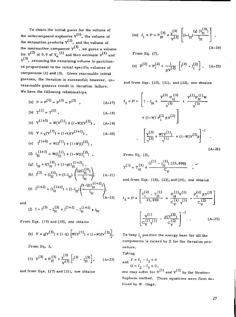
the
the
the
for
TO obtain the initial guess for the volume of
U.ndeconqmsed explosive V(’), the volume of
detonation products V(2), and the volume of
nonreactive component V(3), we guess a volme
V(2) of 0.9 of V.(1)
and then esttiate V(’) and..
V[ 5), assuming the remaining volume is partition-
ed proportional to the initial specific volumes of
components (1) and (3). Given reas enable initial
guesses, the iteration is successful; however, un-
reas enable guesses result in iteration failure.
We have the following relationships.
(a) P = P(’)= P(2)= P(3) ,
(b) T(l) = T(2) 9
(c) V(1+2) = W(v(l)) + (l-w) (V(Z)) ,
A- 17)
A-18)
A-19)
(d) V = ~(V(3)) + (1-x) (V(i+2)) , (A-20)
(e) +1.+2) ~ W(l(l)) + ~1-w)(+2))s
(f) $$+2) = W(#)) + (1-W) (I\2)) ,
(g) + = N&) + (1-ti(#+.2)) ,
()
(ti(f))(h) 1(3) = (#)) + (I-%)
%’(A-21)
(i) ~(1+2)
()
l-ti(#+2))= (~
(1+2), + (~-~) ——
$+. ‘(A-22)
and
(j) I = 1(3) - f)+ 1(1+2) - }+2) + IH
From Eqs. (19) and (20), one obtains
[ 1(k) V = ~V(3)) + (1-X) W(V(l)) + (1-W) (V(2)) .
From Eq. 2,
V(3) 1 - f)], (A-23)(1) P(3) = p:) +2 ‘1(3)
and from Eqs. (17) and (21), one obtains
“)+$ba ~
(m) fl=P. PH
(A-24)
From Eq. (7),
(n) P(2) = P(2)+ --& [1(2) - 1(2)],i i
(A-25)
and from Eqs. (23), (21), and (22), one obtains
[
v(’) p (3) V(l)p(l)w
f2 =P= I- %+~(3)H + Y( 17
+ (1 -w) diz) pv(2) 1
(A-26)
From Eq. (3),
(1(1)- ;)) (23,890) . .. i..
T(l) =T(l) ~H
—,
Cv
and from Eqs. (18), (23), and(25), one obtains
f3. P.[
T(2) - ~(l)i H..—
23, 890L
+
p(l) (1)Hv—— —~(1) pv
[
v(l)
-1
-1- J@ 2))
(A-27)~(l)y(l)
vC:) “
To keep Ii positive the energy base for all the
components is raised by Z for the iteration pro-
cedure.
Taking
F=fl -f3=oand
G=f2 -f’=o,
one may solve for V(l) and V(2) by the ~ewton-
Raphson method. These equations were first de-
rived by W. Gage.
27

The Celling Sequence
CALL HOM2SG (V, S3, S1, G2, RTD)
V, S3, S1, and G2 are dimensioned arrays of
size 14, 23, 23, and17, respectively. S3 is the non-
reactive component, S1 is the undecomposed ex-
plosive, and G2 is its detonation products. S3,
S1 have the same values as S in HOM, and G2 has
the same values as G in HOM.
v(1) v Input
V(2) I Input
V(3) X (S3 mass fraction relative to S1 + G2
+ S3)
V(4) W (S1 mass fraction relative to S1 +G2)
v(5) P output
V(6) v(3) output
v(7) v(1) output
V(8) V(2) output
V(9) I(3) output
V(lo) J.(l) output
V(n) I(2) output
V(l 2) T(3) output
V(13) T(1) output
V( 14) T(2) Output
IND = O for normal exit
= -4 for iteration error.
APPENDIX B
DERIVATIONS OF MOMENTUM, ENERGY,
AND MASS MOVEMENT EQUATIONS )
In this appendix we present the derivations of the difference approximations used to describe the
momentum and energy equations with the transport terms dropped. The method used for mass movement
is also described in detail. This is the OIL method described in Refs. 4 and 11.
1. DERNATION OF MOMENTUM EQUATIONS
w NwlLP~=- 3ZP3, Q3
[3
F$; j
Q2, P2 ‘ P4, Q4
i$ j
.—Pl, Q1
“nv. vn .--=--.=
L J 1>J[ 1(P+q)~j~-(p+q)~j-&
P:, j #
(P:. +P;’ (P:, .+P3)P? =
12j+$ = 2 2
(P; j + Pi)Pn
hj-$= ‘— 2
‘nv. .=vn
[
-–~ ‘3; ‘1 +Q31, J l>j P. 15Z
- Qli ji, j
I,j 1
28
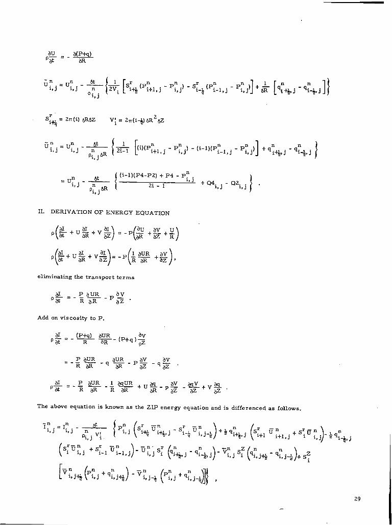
S= = 2n(i) @6Z1++5 v! = 2~(i-+) 6R26Z
1
-nu @=Un -—ilj I,j ,{[
+ (O(p~+l j - P~j) - (i-l)(Pn 1-P:j)+q;%jP:j@ , I-l, j - ‘~+ j
‘?/
ijt
{
(i-l )( P4-P2) + P4 - P; j.un .-—
11J + Q4. - Q2.p;, j m
2i-1 11j/lvj “
II. DERIVATION OF ENERGY EQUATION
eliminating the transport terms
Add on viscosity to P.
a (P+q) auRp~.-—F- R (P+q);
The above equation is known as the ZIP energy equation and is difference as follows.
29

v! = 2~(i -+) &U26Z1
Sz =.2~(i-*)m2i
(U1 = u? +finl-l, j I-l, j )
(U2= Un +:?
1+1, j 1+1, j )
(V1 = v? +?.n.
l, j-1 l, J-1 )
(V2 = v? +;. .
1, j+l 1, J+l)
(T3 = U? +fin
h j h j )
(T1 = Vn
)i,j+w .
lSJ
M.
{
Pn . C24. .I-:, j i- I. —’~ [(i) (T3 + U2) - (i - 1) (T3 - ul)l+ ~&& [(i +*) U2 - (i-#T3]. - — 2(2i-l)@ISJ n
P.h j
Q 2i, j
- 2(2i-l)@ ‘(i - l*)U1 - ‘i - @T3’ ‘* [P;j(v2 11-Vl~ + Q3i, j(V2 - Tl) + Qli, j(Tl - Vl) .
30

‘n ([.I?. .-#- Zj- UzU2 + 2T3 + U1 Q4. .
Iis j I) J
- ul + ---—-21-1 ][
+* U2 -’1’3+ ~+
i, j 1(2.2.I,j-—@ [U1 1 [-T3-~ +~ P;j (V2 - Vl) + Q3
i,j ‘V2- Tl) + Ql
82 1)i,j(T1 - Vl) .
III, DERIVATION OF MASS MOVEMENT EQUATION
The Ofi ~etiod4, 11for velocity weighting is derived below.
i-l, j iJj
+ AR—
a
The mass to move across b is between a and b
velocity at d. Using the first two terms of the
b
where d = b - a; thus, d . 7i~t where %is the weighted
Taylor series at a distance - d from b, we expand
u. + u.l-l, j 1$ju=——
2
Substitute A = ;At and solve for ~.
u. + u.I-l$j 1u.
/( (
~+&2 AR
- u.))
i- u.. .l-l, j 1*J
Mass moved = S Ad/2° i, j
~ At where S—— dis surface area at iAR - $d, so for cylindrical geometry S
d/2=,Zn (i@ - @)Az.
G@We define A= d/AR = — for convenience; therefore,
AR
sdJ2 = 2n(iAR -+(A) (AR))AZ
.211AR(i-&.JAz
.&(2i-&)Az.
Mass Moved . ITAR(2i - A) Az~i-l, jfiAt.
The volume of cell i-1, j is
l-l]j ‘Ni’R)2U ‘nti-l) ‘)zmv.
=rr(2i - 1) ARzAz
31

Diwf .
I.
ful
~(2i-~hZ~i-1 .~At for slab geometry ~. 1.0, which can beMass Moved >JUnit Volume =
~2i - 1) AR2AZ “shown by letting Sd,2= ARAZ and Vi-l, j = AR2AZ
0= ‘d/2 = @ and Vi-l, j = ARAZ.
DM=~-()
ii&(2i - 1) ‘i-ljj ~
APPENDIX C
2DE CODE
COMPUTER TIME
The time required to run a calculation is use-
in evaluating a numerical technique. Because
the compute r time will vary with the details of
the calculation, it is instructive to have the times
from several sample problems.
The problem of an 85 -kbar shock in nitrometh-
ane interacting with an aluminum rod was cal-
culated using 100 cells in the Z direction and 50
cells in the R direction. The aluminum rod had
a radius of 25-cell widths. The calculation re -
quired 9.64 min of CDC 76OO time to complete
the calculation to 446 cycles. The average time
per cycle was 1.297 see, and the average tfie
per cell per cycIe was O. 00026 sec.
The problem of an 85 -kbar shock in njtrometh-
ane inte ratting with an aluminum slab and then
the aluminum interacting with air was calculated
using 180 cells in the Z direction and 3 cells in
the R direction. The calculation required 4.916
min of CDC 76OO time to complete the calcula-
tion to 2323 cycles. The average time per cycle
was O. 127 sec and the average time per cell per
cycle was O. 000235 sec.
A reasonable estimate of the computer time
required for the 2DE code is between O. 0002 and
O. 0003 sec per cell per cycle.
IL MIXED-CELL TREATMENT
Up to 15 materials can be accommodated by
the code. However, at present, equation-of-state
DETAILS
routines allow only two materials in a ceil simul-
taneously.
Each mixed cell (cell containing more than one
material) is flagged in its cell identification word
(CID) by an index pointer, which is the FORTRAN
index of a material identification word in the mixed-
cell table (CMT or MT), A material identification
word exists in the CMT table for each material in
a mixed cell. This word contains (1) an integer
that identifies the material and (2) index values
that determine subsequent and previous material
identification words for other materials in the
mixed ceI.I. Quantities ass ociated with a given
mate rial are indexed relative to material identifi-
cation words. When mixed-cell information is
used or modified, it is first moved into smaller
processing arrays and, if modified, moved back
into the CMT tables. When a material is depleted
from a mixed cell, the space in the mixed-cell
table is made available for further use. Formats
for the cell identification word and the mixed-cell
table are documented in the code listing. Mass is
moved from the donor cell to the acceptor cell on
the basis of the fraction of material in the acceptor
cell, which is common to the donor cell. If the
acceptor and donor cells do not contain any common
materials, then mass is moved according to the
mass fra ctions of mate rids in the donor cell.
Energy and specific volumes are partitioned by
the mixed-cell equations of state. E the acceptor
cell contains only one material and the donor cell
32

also contains this material, then the amount of
mass move d is done on the basis of this partition.
ing. The internal energy is similarly handled.
This calculation and storage of the re suits is
handled by the subroutine ‘1CM.XD!I which requires
the indites of the donor and acceptor cells and the
amount of mass moved per unit voliune of the donor
cell in its calling sequence. This routine deals
with abs olute mass movement and because other
routines deal with tk change in mass per unit vol-
ume, this mass is calculated using the donor cell
volume.
I.U.. DATA PROCESSJ3TG
Storage requirements for individti problems
are minimized by a preprocessing routine called
VARYDIM. This routine processes generalized
FORTRAN common, dime nsion, equivalence and
data statements, These statements have the same
format as ordinary FORTRAN statements except
that integer quantities may be replaced by either
a variable or an arithmetic statement. The restit
of an arithmetic statement being a simple left-to-
right evaluation of the operations in the statement.
The operands may be either integers or variable
names that represent integer values, The results
of this routine are output to a file of compilable
FORTRAN statements and update control cards.
The FORTRAN statements are distributed through-
out the code by CDC system update routine. II-I
general, only a small number of changes are re-
quired to completely modify the storage require-
ments for a specific problem.
Preprocessing dimensions before the code is
compiled allows flexibility in the size of arrays
that must be maintained in addressable memory.
Because the row R dimension can be set before the
code is compiled, processing of arrays that con-
tain cell and intermediate quantities are on the ba-
sis of this dimension being fixed at execution time.
The se quantities are maintained in external storage
and moved into core for processing andlor output.
The problem grid is divided into NJMAX core in-
crements for a fixed number of rows in the Z di-
rection at the discretion of the user.
The routines RDCELLS and WCELLS handle
1/O on the basis of reading or writing rows in
the Z direction for a specified core increment.
These routines are programmed for the CDC 6600
or 76OO using extended core storage or large core
memory. Disk can also be used.
Processing control for the five phases of the
code is accomplished by subroutine CONTROL.
The grid is processed from left to right, bottom
to top. Because the processing of a row often re-
quires information contained in a previous row,
reading, processing, and storing the results are
staggered.
Rows are indexed from J . 1 to JMAX in
addressable storage. Initially, the first two rows
are read into core and the first row is processed
(case 1). Then rows 3 through JMAX are read
and rows 2 through JMAX-1 are processed (case
2). The first JMAX-2 rows are written to exter-
nal storage, and two rows from the next core in-
crement are read into rows 1 and 2 of core allow-
ingprocessing of row JMAX and row 1 of the next
core increment (case 3). After rows JMAX and
JMAX-1 are written to external storage, the pro-
cess is looped back through cases 2 and 3 until
the final core increment where the last row of the
grid is processed and written as a special case
(case 4).
IV. PROCESSOR INPUT
Generalized FORTRAN statements prepared
for the preprocessing routine VARYDIM modify
storage requirements for the code 2DE. The user
must define the preprocessor variables used in
these statements. Preprocessor variables are
input to the routine VARYDIM in a format-free
fashion by the specification of the variable name,
an equal sign, and the integer value of the variable.
All 80 columns of the card are used. A $ terminates
33

pr oces sing allowing the remainder of the card for
comments. Since variables are used in left-to-
right arithmetic, their values must be defined be-
fore they are used to define other variables.
The following preprocessor variables must:,
have values.
For cell storage:
IMAX Number of cells in the R direc-
tion.
.rMAx Number of ceils in the Z direc-
tion.
NJMAX Number of core increments.
For material storage:
NM Number of materials.
Number of materials requiring
HOM equation of state parameters
(usually equsl to NM).
For rectangular storage:
NRI Number of rectangular intervals
on the R axis.
NZJ Number of rectangular intervals
on the Z axis.
For mixed-cell information storage:
NTRYS Estimated total number of mater-
ials for all cells containing more
than one material, (Note that
when a material is depleted in a
cell, storage is again available
for more information. )
Example: If there are N mixed
cells and each of these contain
tsvo materials, then NTRYS = Z*N
For circular input storage:
NCIR Number of circles.
For two-dimensional plot storage:
NGRPHS
NPL@TS
NTYPES
Total number of graph types
available (default = 8).
Number of plots produced each
time cycle.
Number of graph types used by
the code. (default = 8).
NC@NL Maximum number of contour
lines allowed in a given cell
at the same time (default =
20).
For one -dimensional plot storage:
KPLlbTS Number of plots produced
each time cycle.
IXZ Number of cross-sections
parallel to the Z axis.
JXR Number of cross-sections
parallel to the R axis.
AU of the above must have a value of at least
one because they are used to form dimension and
common statements.
v. INPUT AND OUTPUT
Except for input required to define storage,
problem input is accomplished using the system
NAMELIST input.
The two NAME LIST names !iDump!! and
l!Gener~l! per~k to input required by the d~p
routine and the general input for the problem.
IIDDPI! ~put is read by routine EULER2D. “Gen-
eral!! input is read by s ubroutike INPUT.
A. General Input
The following FORTRAN variables are used
for the problem input. The integer subscript K
must be consistent for each material and must not
exceed the value of the preprocessor variable
(NM) that defines storage.
Problem identificatioru
ID Cent aim up to 70 Hollerith
characters printed on the
output listing, film listing,
and graph titles.
Material descriptions:
NAME(K) Material names, each name
consisting of up to 10 Hone-
rith characters,
KMH(K) Assigned material number.
VISC(K) Viscosity constant,
IREACT(K) . T. or . F. reaction flag for
the Arrhenius rate law.
34

IJ-IE(K)
S(l, K)
G(l, K)
RH@O(K)
AC TE(K)
FREQ(K)
MTYPE(K)
DICE
. T. or . F. flag for a high
explosive.
Equation- of- state pararnete rs
for the solid.
Equation- of-state parameters
for the detonation products.
Initial density, used only for
skipping tests.
Activation energy.
Frequency factor.
3HGAS for a gas, 4HS~LID
for a solid, 2HHE for an ex-
plosive. These flags are
initialized for a solid.
. T. allows the code to elimi-
nate a component from a cell
if the component is isolated.
Problem description: Cells are processed
using either slab or cylindrical geometry. Boun-
dary types are numbered starting at the bottom of
the grid and increasing in a clockwise direction for
the four grid boundaries.
SLAB
Boundary types:
B1
B2
B3
B4
. T. indicates slab geometry.
(Default value = . F. for cy-
lindrical geometry. )
Boundary 1 (default value .
6 HPIST@N) .
Boundary 2 (default value =
4HAXIS) .
Boundary 3 (default value =
9HcbNTmuuM).
Boundary 4 (default value =
9Hc@NTINuuM) .
Piston applied values:
PAPP Applied pressure.
WAPP Applied mass fraction.
EAPP Applied energy.
VAPP Applied velocity,
MAPP Applied mass.
Miscellaneous:
MINWT Minimum cell reaction
FREPR
temperature (default
value = 1000).
MINGRH@ Constant for handling free
surfaces, eliminating false
diffusion (default value =
o. 5).
Mass is not moved unless
the pressure of the cell
from which mass moves is
greater than this variable
(defatit value = O. 0005), Or
a tensibn flag has been set.B. Rectangular Input
The problem” grid is divided into NR rectangles
indexed from left to right, bottom to top. AU cell
quantities are initialized from this rectangular in-
put.
Rectangles are form d by dividing the R and Z
problem directions into NRI and NZJ intervals. If
M and N index these intervals, then
NR
RW(M)
ZW(N)
Ill(M)
JZ(N)
DELR(M)
DE LZ(N)
Number of rectangles.
Width of the M th interval.
Width of the N th interval.
Number of cells in the M th
interval.
Number of ceJls in the N th
interval.
Cell width in the M th
interval (currently the same
for all intervals).
Cell width in the N th inter-
val (currently the same for
all intervals).
For the L th rectangle:
KMAT(L) Material K for the rectan-
gle.
RHO(L) Initial cell density,
PO(L) Initial cell pressure.
TO(L) Initial cell temperature.
U 0( L) Initial cell velocity in the
U direction.
VO( L) Initial cell velocity in the
V direction.
35

WO( L) Initial cell rnass fraction.
DELT(L) Time increment.
C. Circular Jnput
Cells can be initialized by defining NCI.R con-
centric circles. The radial difference between
circles must be at least larger than the large st
diagonal of any cells contained between the differ-
ence.
RO R coordinate for the circle
centers.
Zo Z coordinate for the circle
centers.
For the L th circle, indexed from the largest
to the smallest,
RAD(L)
RH@OC(L)
KCIR(L)
IOC(L)
UOC(L)
VOC(L)
WOC(L)
D. Output
Radius of the L th circle.
Density of the L th circle.
Material K for the L th
circle.
Energy of L th circle.
U velocity of L th circle.
V velocity of L th circle.
W of L th circle.
Output for specific cycles is directed to both
the printer and to film. This output is controlled
by the specification of an initial cycle, an incre -
ment between cycles and a terminating cycIe. In-
put information is output unless the print or film
terminating cycle is set to zero.
Pcs Starting print cycle (de-
fault value = 1).
PCI Print cycle increment (de-
fault value = 50).
PCE Terminating print cycle
(default value = 5000).
FCS Starting film cycle (default
value = 1).
FCI Film cycle increment (de-
fault value . 25) .
FCE Terminating film cycle (de -
fault value = 5000).
Plot cycles are specified by the above film
cycle specifications unless specified by the follow-
ing variables:
PLTS Plot cycle start.
PLTI Plot cycle increment.
PLTE Plot cycle end.
2DE is programmed to produce isoplots (con-
tour plots ) of values associated with each cell. At
present eight isoplots are allowed. Up to 10 indi-
vidual plots per problem time cycle can be pro-
duced by input control. Any or all of the is oplots
associated with cell quantities can be plotted on an
individual plot frame, Contour intervals, grid
maximum, and grid minimum can be modified.
Default values are documented in the code. E L
indexes the plot frame, then
IS6PL@T(L) Determines which isoplots
will be produced on the L th
plot frame.
1 = isotherm, 2 = isobar, 4 = isopycnic,
8 = energy, 16 = cell U velocity, 32 =
cell V velocity, 64 = W mass fraction.
are
To get more than one plot per frame, values
added together for LS~PL@T(L ).
If M indexes the is oplot type, then
GMM(M)
GMIN(M)
GDELTA(M)
NPL@TS
Maximum value plotted for
the M th is oplot type.
Minimum value plotted for
the M th is oplot type.
Contour interval for the
M th isoplot type.
Number of two-dimensional
plots . This variable is set
by the preprocessor; how-
ever, if it is modified here
by being set equal to zero,
all two-dimensional plots
will be eliminated from the
Outp Ut.
36

NTRFCE If . T. , positions of mixed
cells are plotted with an
asterisk.
2DE produces one-dirnensional cross-section
plots of the cell quantities as a function of R or Z.
The total number of one -dimensional plots, the
number of cross sections parallel to the Z axis
(IXZ), and the number of cross sections parallel
to the R axis (JXR) are fixed by the preprocessor.
Default values that determine which cell quantities
are plotted, and the location of cross sections on
the grid are documented in the code. A cross
section parallel to an axis is specified by a cell
index on the other axis. If M indexes plots and L
indexes cross sections, then
IC~N(L)
JC@N(L)
PTYPE(M)
KPL@TS
Contains IXZ indices that
define cross sections par-
allel to the Z axis.
Cofiains JXR indices that
define cross sections par-
allel to the R axis.
Determines which cell quan-
tity is plotted.
Number of one-dimensional
plots . This variable is set
by the preprocessor; how-
ever, if it is modified here
by being set equal to zero,
all one -dimensional plots
will be eliminated from the
output .
Scaling of plotted outputi 4020 grid coordi-
nates can be used to scale graph output. Default
values are for a square grid.
IXL Grid left coordinate
(default value = 120).
IXR Grid right coordinate
(default value = 980).
IYT Grid top coordinate
(default value = 50).
IYB Grid bottom coordinate
(default value = 910).
E. Debug Features
Debug routines display the results of each
phase of the code, mixed cell processing, and the
dump routine. The following variables control the
Ou I.put.
DEBUG(L)
DBS
DBI
DBE
For the logical variables
L= 1 through 5, phases 1
through 5 are debugged,
Flags 6 ad 7 produce dump
information for the mixed-
cell and dump routine.
Cycle control star ting the
debug dump.
Cycle increment for dump-
ing.Terminating cycle for durnp-
tire
The
%.
Unless specific cells are designated, the en-
grid calculation is printed for a debug cycle.
following variables restrict printing to par-
TAPE
DTI
SECS
titular cells.
IGS Starting radial or I index.
IGE End rng radial or I index.
JGS Starting Z or J index.
JGE Ending Z or J index.
F. Restart Features
The user has the option of dumping at speci-
fied running time increments or of dumping at
specified problem cycles. Uses the N.AMELIST
rmme ‘! Dump. ‘!
DCYCLE Initially zero. Set to the
probIem cycle for picking
Up dumps.
COMMENT Up to 70 Hollerith charac -
ters that go to the printer
and express file.
Up to 10 Hollerith charac-
ters for a dump tape label.
Dump time increment (de -
fault value = 300 see).
Tolerance that allows time
for the last dump before
I
37

the problem is terminated
by a time limit.
For the optional method of dumping, the fol-
lowing variables must be specified.
DMPS Starting dump cycle. (If
DMPI . 0 the alternate
method of time increment
dumping is used. )
DMPI Dump cycle increment.
~. Time Step Modification
At specified cycles the time step (DELT) can
be modified by a multiplication factor ( TFCT). Up
to 5 modifications are allowed.
NTCY Problem cycle at which
the time step is modified.
TFCT Multiplication factor.
H. NAMELIST Types
NAMELIS T input requires that input variables
and input values agree in type. The types are
listed below.
INTEGER
MTYPE
KMAT
IR
JZ
KCIR
Pcs
PCI
PCE
FCS
FCI
F CE
PLTS
PLTI
PLTE
LS@PL@T
NPL@TS
ICON
JC@N
PTYPE
VCNT
KPL@TS
IXL
IxR
IYT
FLOATING POINT
VISC Po
s TO
G UoRH@O Vo
ACTE Wo
FREf2 IO
RHO DELR
IOC DE LZ
38
IYB
DBS
DBI
DBE
IGS
NCYLIM
IGE
JGS
JGE
DCYCLE
DMPS
DMPI
Uoc
RG
DELT
GMAX
GMIN
GDIZLTA
DTI
SECS
DMPE
NR
NRI
NZJ
KMH
NTCY
KC’IR
NC@NL
IXL
IXR
IYT
IYB
PAPP
Voc
RW
EAPP
. WAPP
VAPP
MAPP
MINWT
MINGRHO Woc RH@OC Zo
FREPR Zw RO RAD
TFCT DTI
LOGICAL
IHE SLAB
IREACT NTRFCE
DEBUG DICE
HOLLERITH
ID B1
NAME B2
C@MMENT B3
TAPE B4
MTYPE
VI. STORAGE RECNH.RMENTS—
On the CDC 7600 computer the 512, 000 words
available in large core memory (LCM) are shared
by the user, the program file set buffers, and the
system monitors. Because the system require-
ments are subject to change, only rough estimates
can be given for the problem storage limitations.
The code can process approximately 20, 100
cells if the buffers are set to minimum vslues.
U more cells are needed, the disk can be used.
REFERENCES
1.
2.
3.
4.
5,
M. Rich, 11A Method for Eulerian FluidDyn-ics, It LOS ~amos Scientific Laboratory
report LAMS-2826 (1962).
Richard A. Gentry, Robert E. Martin, andBart Jo DAY, !!~ Euler ian Differencing Me th-
od for Unsteady Compressible Flow Prob-1 87 (1966).~ems, it JO Computitionti Phys. _~
William R. Gage and Charles L. Mader, lt2DE -A Two-Dimensional Eulerian HydrodynamicCode for Computing One Component ReactiveHydrodynamic Problems, ” Los Alamos Scien-tific Laboratory report LA-36 29-MS ( 1966).
w. E. Johnson, “OIL: A Continuous Two-Dimensional Eulerian Hydrodynamic Code, “General Atomic Division of General DynamicsCorporation report GAMD-5580 (1964).
Charles L. Made r, !! The Time-Dependent
Reaction Zones of Ideal Gases, Nitromethaneand LiquidTNT, 11Los Alamos Scientific
Laboratory report LA-3764 (1967).
6. Charles L. Mader, {1The Two-Dimensional
Hydrodynamic Hot Spot - Vol. IV, “ LOSAlamos Scientific Laboratory report LA-3771(1967).
7. Charles L. Mader, “Numerical Calculationsof Detonation Failure and Shock kitiation, ‘ !Fifth Symposium (International) on Detonation,Office of Naval Research report DR-163 (1970).
12. C. W. Hirt, !t-propos~ for a Mtiti.materi5.1~
Continuous Eulerian, Computing Method, “Personal communication (1969).
13. Laura J. Hageman and J. M. Walsh, “=LP -A MuMi-Material Eulerian Program for Com-pres sible Fluid and Elastic-Plastic Flows inTwo Space Dimensions and Time, ” Systems,Science and Software report 3SR-350 (1970).
8. Charles L. Mader, I!One- ad Two-~en- 14. Charles L. Mader and William R. Gage,sianal Flow Calculations of the Reaction Zones !IFOR TR~ Sm - A One-Dimensional Hydro-
of Ideal Gas, Nitromethane and Liquid TNT dynamic Code for Problems which IncludeDetonations, II Twelfth Symposium (Interna- Chemical Reactions, Elastic-Plastic F1ow,tional) on Combustion (WiLliarn and Wilkins, Spalling, and Phase Transitions, “ LOS Alamos1968), p. 701. Scientific Laboratory report LA-37 21J(1967).
9. Charles L. Mader, “Numericsl Calculationsof Emlos ive Phenomena. 11in Comnuters and. .Their Role in the Phys ica.1 Sciences, A. Tauband S. Fernbach, Eds. (Gordon and BreachScience Publishers, New” York, 1971), p. 385.
10. Charles L. Mader, !l~o-Dimension~ Hydro-dynamic Hot Spot, Vol. II, “ Los AlamosScientific Laboratory report LA-3235 ( 1964).
11. W. E. Johnson, 1!Developme nt and Applicationof Computer Programs Related to Hype rveloc -ity ~Pact, 18Systems, Science and Software
report 3SR-353 (1970).
15. Charles L. Mader, Roger W. Taylor, DouglasVenable, and James R. Travis, “Theoreticsand Experimental Two-Dimensional Interac -tions of Shocks with Density Disc ontinuities, “Los Alamos Scientific Laboratory reportLA-3614 (1966).
16. William R. Gage and Charles L. Mader,!! Three -Dirnension~ Carte sian PartiC~e ‘h-
Cell Calculations, I! Los ~a.mos sCkIIt~k
Laboratory report LA-3422 (1965).
ALT/je: 453(200)
39