ETF Arbitrage under Liquidity Mismatch∗

Kevin Pan

Harvard University

Yao Zeng

University of Washington

February, 2017

Abstract

A natural liquidity mismatch emerges when liquid exchange traded funds (ETFs) hold

relatively illiquid assets. We provide a theory and empirical evidence showing that this liquidity

mismatch can reduce market efficiency and increase the fragility of these ETFs. We focus on

corporate bond ETFs and examine the role of authorized participants (APs) in ETF arbitrage.

In addition to their role as dealers in the underlying bond market, APs also play a unique role

in arbitrage between the bond and ETF markets since they are the only market participants

that can trade directly with ETF issuers. Using novel and granular AP-level data, we identify

a conflict between APs’ dual roles as bond dealers and as ETF arbitrageurs. When this conflict

is small, liquidity mismatch reduces the arbitrage capacity of ETFs; as the conflict increases,

an inventory management motive arises that may even distort ETF arbitrage, leading to large

relative mispricing. These findings suggest an important risk in ETF arbitrage.

Keywords: Authorized participants, arbitrage, corporate bond, exchange-traded funds,

liquidity mismatch.

JEL: G12, G14, G23.

∗We thank Zahi Ben-David, Hank Bessembinder, Darrell Duffie, Robin Greenwood, Sam Hanson, Wei Jiang,Adi Sunderam, and in particular John Campbell, Andrei Shleifer, Jeremy Stein, and Luis Viceira for many detailedand helpful suggestions. We thank conference and seminar participants at Duke Fuqua, Harvard, UW Foster, andPacific Northwest Finance Conference for helpful comments. We particularly thank Alie Diagne, Ola Persson andJonathan Sokobin of the Financial Industry Regulatory Authority (FINRA) for providing us with privileged accessto a proprietary TRACE data set; we also thank the Depository Trust & Clearing Corporation for providing dataon ETF arbitrage baskets. We are also grateful to two major ETF sponsors for sharing data on their authorizedparticipants, as well as their respective capital market and institutional services teams for insightful conversations.Finally, we thank market participants at BNP Paribas, Citigroup, Emeth Partners, Harvard Management Company,and Susquehanna for conversations that helped us better understand ETF arbitrage. Pan acknowledges the financialsupport of the NSF Graduate Research Fellowship (DGE1144152) and Doctoral Dissertation Research ImprovementGrant (1628986).

1 Introduction

Corporate bond exchange traded funds (ETFs) are characterized by a liquidity mismatch: while

the ETF trades on an exchange, the underlying corporate bonds are traded bilaterally in opaque

over-the-counter markets.1 Proponents of these financial products have argued that liquidity mis-

match is not an important risk by highlighting the abundant liquidity created in the ETF market

and the existence of the ETF arbitrage mechanism. ETFs are thus a positive innovation that

improves price discovery and market liquidity in an otherwise opaque and illiquid bond market.2

In contrast, academics and financial regulators have begun to point to negative implications of

ETFs. Regulators and some market participants have hypothesized that liquidity mismatch could

lead to large price discrepancies and fragility in both the ETF and underlying bond market.3 A

recent academic literature has also highlighted potential risk implications of ETFs from a market

stability and shock transmission perspective; this literature however has focused predominantly

on equity ETFs where there is no liquidity mismatch.4 Despite the debate, the risks of liquidity

mismatch in corporate bond ETFs and the underlying mechanism giving rise to these risks are

unexplored. Can ETFs written on illiquid assets “fail” at times?

To address this question, we highlight that the natural liquidity mismatch in corporate bond

ETFs results in a unique inventory risk. To align the price of the ETF and the ETFs’ portfolio

of corporate bond holdings, authorized participants (APs) perform arbitrage (i.e., ETF creations

and redemptions) by buying the lower-priced asset, simultaneously selling the higher-priced asset,

and directly trading with the ETF issuer at the end of a trading day. Because corporate bonds

are illiquid and cannot be immediately transacted without incurring large price impacts and high

costs of trade, APs hold bond inventory. As a result of the need to transact in the underlying

over-the-counter (OTC) bond market and maintain bond inventories, APs are also large leveraged

broker-dealer institutions designated for bond market-making. The dual roles of APs as financial

intermediaries active in ETF arbitrage (APs are the only intermediaries able to perform ETF

creations and redemptions) and corporate bond market-making generates a new tension. Because

APs are not contractually bound by legal obligations to perform ETF arbitrage, APs may occa-

1ETFs are investment funds that are traded on stock exchanges. The fund hold the assets of a stated index andattempts to closely track the return profile of that index. ETFs combine features of two common investment funds– open-end and closed-end mutual funds. Section 2 presents a description of the relevant institutional details.

2See Madhavan (2016) for a discussion of the benefits of ETFs to the efficiency of the underlying markets.Industry reports have also argued for a “non-displayed” secondary market liquidity as a feature of exchange-tradedfunds. See BlackRock Viewpoint July 2015 “Bond ETFs: Benefits, Challenges, Opportunities” and SSGA SPDRpublication “Underneath the Hood of Fixed Income ETFs: Primary and Secondary Market Dynamics.”

3For example, the former Commissioner of the U.S. Securities and Exchange Commission, Daniel Gallagher,argued that the lack of liquidity in corporate bond markets may pose systemic risks to the economy and corporatebond mutual funds and ETFs may be a potential channel. See http://www.bloomberg.com/news/articles/2015-03-02/corporate-bond-market-poses-systemic-risk-sec-s-gallagher-says.

4We discuss this literature in detail in the literature review.

1

sionally become liquidity seekers (perhaps as a result of their bond market-making activities) and

withdraw from ETF arbitrage rather than acting as liquidity providers in the ETF market.

This paper formulates the logic above and shows new evidence that ETF arbitrage is subject

to several frictions in both the underlying bond market and the ETF market. These frictions can

reduce the intensity of ETF arbitrage, resulting in persistent relative mispricing and potential

market fragility. These frictions arise more acutely in the corporate bond ETF setting (relative to

equity ETFs where there is no liquidity mismatch) because the dual roles of financial intermedi-

aries as both ETF arbitrageurs and as bond dealers conflicts more strongly when the underlying

asset is relatively illiquid. We formalize this conflict using a stylized model of ETF arbitrage that

highlights the important role liquidity mismatch plays. The model describes the key role of cer-

tain financial intermediaries – authorized participants (APs) – in the ETF arbitrage mechanism

and generates predictions for how market volatility, liquidity mismatch and the APs’ corporate

bond inventory imbalances interact to limit the risk-bearing capacity of these APs. Combining

several unique datasets novel to the literature, we find empirical evidence consistent with the

model predictions. We show empirically how liquidity mismatch and bond inventory positions

interact to lower APs’ sensitivity to arbitrage opportunities, and present evidence on the impact

of realized AP arbitrage on corporate bond returns and liquidity.

To begin, we present a stylized model of ETF arbitrage that shows how a specific “failure” of

ETF arbitrage can occur as a result of two opposing effects: an arbitrage effect and an inventory

management effect. The model focuses on three institutional features: 1) ETF creations and

redemptions can only be performed by APs; 2) liquidity mismatch exists between corporate

bonds and the ETF; and 3) APs act both as ETF arbitrageurs and as bond dealers and they

may hold existing bond imbalances initially. In the model, when the ETF price deviates from

the price of the underlying portfolio of bonds, APs (potentially) trade to arbitrage the relative

mispricing. In a frictionless benchmark, for any given ETF premium (discount), APs short (long)

the ETF, long (short) the underlying basket of bonds, and then create (redeem) ETF shares with

the ETF issuer at the end of the trading day to unwind the arbitrage positions. Importantly,

in this frictionless benchmark, the ability to trade with the ETF issuer end-of-day allows APs

to more aggressively perform intraday arbitrage and hence increases the likelihood of consistent

relative pricing. However, our model shows that liquidity mismatch generates an important

conflict between APs’ role as bond dealer and ETF arbitrageur with the potential to limit APs’

arbitrage capacity and possibly leading to even larger relative mispricings. Two effects arise: an

arbitrage effect and an inventory management effect.

When the absolute magnitude of APs’ initial bond imbalances is small, APs perform arbitrage

across markets to close relative mispricings: the arbitrage effect. APs are willing to close rela-

2

tive mispricings when the marginal benefit of expected arbitrage returns outweighs other costs,

including suboptimal inventory levels. However, AP arbitrage remains far from frictionless and is

limited by various frictions related to liquidity mismatch. For any given initial relative mispricing,

the sensitivity of ETF arbitrage by APs is declining in market volatility, bond market illiquidity

and costs of trade. Intuitively, when limits to arbitrage between the ETF and the underlying

bonds become more severe, APs establish smaller arbitrage positions intraday and hence perform

less ETF creations and redemptions resulting in higher residual relative mispricings.

In contrast, when the absolute magnitude of APs’ initial bond imbalances are large, the inven-

tory management effect – the motive to trade towards an optimal bond inventory level – becomes

dominant and may even distort ETF arbitrage. While APs may still create and redeem ETF

shares, ETF arbitrage may go in the opposite direction than what would be implied by the initial

relative mispricing. Specifically, APs may choose to create (redeem) more ETF shares where they

have extremely positive (negative) bond inventory imbalances, regardless of the initial price dis-

crepancy. Surprisingly, the model suggests that APs do even more ETF creations and redemptions

when bond volatility increases or as the market becomes more illiquid. Intuitively, APs strategi-

cally use ETF creations and redemptions not to correct relative mispricings but to unwind bond

imbalances, reduce existing inventory risks and facilitate future market-making in their role as

bond dealers. In this sense the ETF arbitrage mechanism becomes “distorted” – creations and

redemptions are disconnected from fundamentals (and/or arbitrage opportunities) and gives rise

to the possibility of larger relative mispricings. More precisely, the ETF arbitrage is distorted

not because APs fail to fully optimize. Instead, APs do optimize, choosing to use creations and

redemptions strategically on account of their existing illiquid bond inventory imbalances, thereby

potentially violating the designed intention of the ETF arbitrage mechanism.

We combine several unique datasets novel to the literature to test the model predictions and

draw further conclusions on the asset pricing implications of ETF arbitrage. First, for the sample

period from 2004 to 2015, we obtain historical proprietary lists of APs for each corporate bond

ETF from two ETF issuers. The corporate bond ETFs issued by these two ETF sponsors, which

constitute our data sample, represents on average 83% of the total passive corporate bond ETF

assets under management. Second, we obtain a proprietary version of TRACE, which is a dataset

of all secondary market corporate bond transactions, with dealer identifiers from FINRA which

not only allow us to identify counterparties to trades across time but also allows us to directly

identify secondary market bond transactions of APs specifically. Using these identifiers, we impute

bond order flow imbalances on APs’ balance sheets and identify their impact on APs’ arbitrage

activity. Finally, proprietary time-series data on the daily creation and redemption baskets for

each ETF in our sample identifies the subset of bonds used in the ETF arbitrage and hence

3

allows our empirical design to trace the effect of initial bond pricing and inventory through to

realized AP arbitrage. Overall, the highly granular nature of the data, and the daily-frequency

and cross-sectional variation at the ETF and bond-ETF levels enables us to explore AP arbitrage

in-depth.

We find empirical results that are consistent with the model predictions. First, increases in

market volatility and bond market illiquidity reduce ETF arbitrage, consistent with the arbitrage

effect and its limitations. Withdrawals from arbitrage can be quite large and results in consistent

price discrepancies between ETFs and the underlying holdings of corporate bonds. An increase

of 1% in the ETF premium generates an increase in AP arbitrage by 50 basis points; however,

as market volatility rises, holding fixed the ETF premium, AP arbitrage declines: a one standard

deviation increase in market volatility generates a 10% decline in AP arbitrage. Moreover, the

decrease in arbitrage sensitivity is asymmetrically larger when the ETF premium is negative.

This suggests an asymmetric risk since APs who attempt to correct this relative mispricing would

become even more exposed to risks arising from liquidity mismatch.

Second, bond inventory generates unique risks to ETF arbitrage through the inventory man-

agement effect. When APs experience extreme bond inventory imbalances, APs’ creation and

redemption activities become less sensitive to perceived arbitrage opportunities, and more sen-

sitive to the amount of their bond inventory imbalances. While ETF arbitrage goes in the di-

rection of the arbitrage opportunity, suggesting that the “ETF arbitrage” channel dominates, a

“differences-in-differences” approach comparing ETFs across inventory scenarios reveals that APs

actually do less (more) net redemptions when inventory shocks are large and positive (negative)

despite there being an ETF discount (premium). Furthermore, consistent with the theory, in such

cases of extreme inventory, the sensitivity of ETF arbitrage becomes more acute as the underlying

corporate bonds become more illiquid and/or market volatility increases. Nevertheless, we do not

find evidence of the complete “failure” of ETF arbitrage – perhaps because such a shock under

extreme inventory scenarios has yet to occur.

Third, outside the model, we find evidence that realized AP arbitrage in turn affects relative

mispricings across markets as well as return and liquidity in the underlying corporate bond market.

Realized AP creation and redemption activities reduce the persistence of relative mispricings and

increases the liquidity in the corresponding arbitrage baskets. However, these effects may become

weaker or even reversed when APs’ arbitrage capacity becomes more constrained due to either

greater liquidity mismatch or AP bond inventory imbalances. Moreover, we find asymmetric

short-term price impacts which are only partially reversed in the case of ETF redemptions. These

findings are broadly consistent with the competition of the arbitrage and inventory management

effect as well as the risk associated with liquidity mismatch in general.

4

Two clarifying points are worthwhile. First, the conflict between APs’ two roles is a direct

implication of the liquidity mismatch between the corporate bond and ETF markets. If the ETF

and the underlying assets are equally (il)liquid, APs’ strategic use of the ETF creations and

redemptions to manage bond inventories becomes moot.5 This suggests a policy need to improve

the liquidity of the corporate bond markets. Second, this paper and our results are silent on

implications for market welfare. We highlight the destabilizing effects due to the unintended

breakdown of the ETF arbitrage mechanism as a result of liquidity mismatch. The distortion of

the ETF arbitrage mechanism reduces the ability to which ETFs can closely track illiquid bond

indices, thereby blunting a proposed benefit of ETFs for end investors. However, this paper does

not offer a complete analysis of the benefits and costs of ETFs from a macro-prudential or welfare

perspective.

Related literature: First, this paper contributes to the recent literature on the risk im-

plications of non-leveraged physical ETFs by highlighting the frictions that arise under liquidity

mismatch – a characteristic we argue is the most important feature of corporate bond ETFs.

We provide both a theory and empirical evidence for this new mechanism and its potential to

generate market fragility via the channel of ETF arbitrage by APs. We are also the first to use

micro-level data on individual APs’ inventory and trading positions to explore ETF arbitrage by

APs. The extant risk literature has focused on equity ETFs, a setting in which liquidity mismatch

is less significant: higher ETF ownership leads to higher intraday and daily volatility (Ben-David,

Franzoni and Moussawi, 2014), return co-movement (Da and Shive, 2016), lower benefits from

information acquisition (Israeli, Lee and Sridharan, 2016) and more persistent and systematic mis-

pricing (Madhavan and Sobczyk, 2014, Petajisto, 2015, Brown, Davies and Ringgenberg, 2016).

Dannhauser (2016) studies corporate bond ETFs and finds that higher ETF ownership lowers

bond yields but has an insignificant or negative impact on bond liquidity; her mechanism focuses

on a migration of liquidity traders from the underlying to the ETF market rather than ETF

arbitrage by APs. Malamud (2015) builds a dynamic asset pricing model of ETFs, which does

feature AP arbitrage but studies equity ETFs and hence ignores liquidity mismatch.6

Second, this paper introduces liquidity mismatch as a new arbitrage friction in the literature

on limits to arbitrage in financial markets.7 While other papers have studied mismatches in asset

5In contrast, in the current corporate bond ETF setting, the ability to manage inventory by transacting directlywith ETF issuers thereby avoiding the transaction in the OTC market constitutes a potentially less costly transactionfor APs and thus provides a rationale for their strategic use of the AP arbitrage mechanism. See a recent Bloombergarticle titled “Wall Street’s New Balance Sheet Is An ETF.” https://www.bloomberg.com/gadfly/articles/2016-05-25/bond-dealers-use-blackrock-junk-etf-as-substitute-balance-sheet.

6Other recent theoretical work on ETFs include Bhattacharya and O’Hara (2016) and Cong and Xu (2016).However these papers focus on indexing effects rather than the mechanism of AP arbitrage.

7A detailed survey is beyond the scope of this paper; typical types of limits to arbitrage include noise-traderrisks (DeLong, Shleifer, Summers and Waldmann, 1990), short-sale constraints (Harrison and Kreps, 1978), equitycapital constraints (Shleifer and Vishny, 1997), and margin and leverage constraints (Gromb and Vayanos, 2002).

5

characteristics, these paper do not focus on limits to arbitrage.8

Third, we contribute to the corporate bond market-structure literature by linking bond dealers’

market-making capacity to the ETF market and show the interaction between ETF arbitrage and

the underlying bond market. While several papers have used the proprietary TRACE data with

masked dealer identifiers as in this paper, our data contains novel additional variables identifying

which dealers are APs. This literature has shown evidence that bond dealer inventory is an

important determinant of corporate bond returns and liquidity;9 this paper provides evidence

that bond inventory is also an important determinant in arbitrage. Our approach is particularly

relevant in the post-crisis economic and regulatory environment: Duffie (2012) points out that

bond market-making is inherently a form of proprietary trading, and Bessembinder, Jacobsen,

Maxwell and Venkataraman (2016), Bao, O’Hara and Zhou (2016), and Dick-Nielsen and Rossi

(2016) show evidence that bond dealers’ inventory management capacity has become more limited.

Fourth, our result contributes to a strand of the literature that highlights how liquidity

providers can occasionally become liquidity seekers with consequences for market stability. Rel-

evant examples include the quantitative traders and hedge funds in Ben-David, Franzoni and

Moussawi (2012), Nagel (2012) who provide liquidity voluntarily, as well as the bond dealers in

Choi and Shachar (2016) who trade against the CDS-bond basis. Market shocks and other time-

varying frictions can raise the expected return from liquidity provision and thus push them to

demand liquidity instead. This paper uncovers a related but less explored logic in the context

of corporate bond ETFs. Since APs have no legal obligation to perform ETF arbitrage, APs

may become liquidity seekers exactly when liquidity provision is called for in the ETF market.

Liquidity provision through the ETF arbitrage mechanism is complicated by APs’ strategic use

of ETF creations and redemptions.

Finally, this paper complements the recent literature on the risks of liquidity mismatch in

open-end mutual funds of corporate bonds. The ETF setting this paper studies is similar to these

mutual funds because ETFs shares can be created or redeemed at the end of the trading day.

Mutual fund outflows predict future declines in NAV (Feroli, Kashyap, Schoenholtz and Shin,

2014) and lead to asymmetric fragility as a result of a concave flow-to-performance relationship

(Goldstein, Jiang and Ng, 2016). Chernenko and Sunderam (2016) find that, following fund

outflows, fund cash holdings are not large enough to meet with redemption demand without

generating price impact, and Zeng (2016) theoretically examine the potential for runs on illiquid

8Duffie (1996), Krishnamurthy (2002) and Vayanos and Weill (2008) suggest that the price difference betweenon-the-run and off-the-run Treasury bonds may come from different short costs. Duffie and Strulovici (2012) modelthe movement of capital between two otherwise identical asset markets with different levels of cash invested. Cespaand Foucault (2014) study liquidity contagion across two markets via market-maker’s cross-market learning.

9Goldstein and Hotchkiss (2011) find that dealers are less likely to hold overnight inventory positions in lessliquid bonds. Friewald and Nagler (2015) show that dealer inventories are related to risk-adjusted bond returns.

6

mutual funds. However, unlike open-end mutual funds, the creation and redemption of ETF can

only be performed in-kind by APs. This leaves a unique channel which this paper investigates.

2 Institutional Background

Exchange traded funds (ETFs), in the context of this paper, refer to unlevered open-end mutual

funds listed on an exchange and invested in a portfolio of physical securities that tracks published

market indices.10 Specifically, we focus on corporate bond ETFs and refer to them simply as

ETFs in the explanation of ETF mechanics. This section first describes the institutional details

of ETF arbitrage and the role of authorized participants (APs), and then argues why liquidity

mismatch – the difference in liquidity between ETFs trading on an exchange and underlying

corporate bonds trading bilaterally in opaque over-the-counter markets – is a critical friction in

corporate bond ETFs.11 The ETF arbitrage mechanism allows a specific subset of intermediaries,

namely APs, to create and redeem ETF shares in exchange for a pre-specified basket of arbitrage

bonds thereby aligning the price of the ETF and its underlying holdings. APs however are not

contractually bound to perform arbitrage; they may withdraw from performing arbitrage as cost

or risk increases.

2.1 ETF Arbitrage Mechanism

ETFs are a hybrid of two common investment funds: open-end and closed-end mutual funds.

An ETF combines the valuation and variable share features of open-end mutual funds, which

can be traded at the end of each trading day for its net asset value (the total net value of all

the assets in its portfolio), with the exchange-traded feature of closed-end funds, which trades

intraday (i.e., within the trading day) at prices that can vary from its net asset value (NAV). One

unique aspect of ETFs is the creation and redemption arbitrage mechanism between APs and ETF

sponsors. ETF shares can be created or redeemed at the end of each trading day for the NAV

of the fund. Unlike traditional open-end mutual funds, however, this creation and redemption

process can only occur between the fund sponsor (i.e., the ETF issuer) and APs.12 This market

10While ETFs typically invest in a portfolio of physical securities, some ETFs track an index by holding derivativesto replicate the performance of the benchmark. These synthetic ETFs are more common in Europe than in theUnited States where they are more heavily regulated. U.S. corporate bond ETFs are predominantly index-trackingand physically replicated (Madhavan, 2016).

11For a more detailed description of ETFs, we refer interested readers to Ben-David, Franzoni and Moussawi(2014) and Madhavan (2016).

12In contrast, any investor in a traditional open-end mutual fund may buy new shares and redeem existing sharesdirectly with the fund at the fund’s NAV. Closed-end funds can be thought of as an extreme case with no ability tocreate and redeem shares. Closed-end funds have a fixed number of shares listed on exchange and may be boughtor sold intraday on exchange but no mechanism to reconcile differences in the exchange traded price and the NAVby adjusting the supply of available shares.

7

is commonly referred to as the primary ETF market and is the market in which changes in ETF

shares outstanding occur.

Importantly, APs are the only market participants active in this primary ETF market by

institutional design. Corporate bond ETFs typically have an average of 25-35 APs, many of

whom are also large, leveraged broker-dealer institutions.13 Despite the barriers to entry as a

result of firms’ market size and business function, APs act competitively in ETF arbitrage.14 In

contrast to APs, non-AP market participants may trade the ETF intraday in the secondary ETF

market but lack the ability to create and redeem shares with the ETF issuers. Instead, non-AP

market participants trade amongst each other and transact at the ETF price.

The unique ability of APs to trade directly with the ETF issuer with in-kind creations and

redemptions represents a cost-effective tool that should encourage ETF arbitrage.15 Specifically,

APs can avoid entering the OTC market at the initiation or close of an arbitrage position and

instead “lock-in” arbitrage profits with the ETF issuer at the ETF’s NAV. While all market par-

ticipants (including APs) can buy or sell ETF shares on the secondary exchange market perhaps

following some statistical arbitrage strategy, only APs can create or redeem shares in-kind directly

with the ETF fund sponsor at the end of a trading day. Given an ETF premium (discount), APs

can secure an arbitrage profit by shorting the ETF (bond portfolio) and going long the underlying

bond portfolio (ETF). In the case of an ETF premium, APs can subsequently unwind any long

positions in the bond portfolio by delivering the ETF’s in-kind creation basket to the ETF fund

sponsor in exchange for ETF shares which are then delivered to settle the short ETF position.

Likewise, in the case of an ETF discount, APs redeem their long ETF position with the ETF

issuer at end-of-day NAV (published at the close of each trading period), and receive the in-kind

redemption basket which can be used to cover the initial short bond position. These in-kind

creation and redemption baskets are published by the ETF issuer to the APs at the end of each

trading day for use the following trading day. In general, the baskets as well as the ETF portfolio

holdings are transparent to APs to encourage ETF arbitrage. The creation and redemption of

ETF shares in the ETF arbitrage mechanism should keep the secondary market price of ETF

shares in a range equal to the expectation of the current fair value of portfolio holdings and

13For example, a publicly available BlackRock publication lists examples of APs executing create/redeem activityfor representative ETFs of BlackRock. APs for LQD (an investment grade corporate bond ETF) in 2013Q1 includedBarclays, Deutsche Bank, Goldman Sachs, JP Morgan, Bank of America Merrill Lynch, Morgan Stanley, NomuraSecurities, and RBC Capital Markets. See BlackRock Viewpoint June 2013 “Exchange Traded Products: Overview,Benefits and Myths.”

14Any U.S. registered, self-clearing broker-dealers who meet certain criteria and sign a participant agreementwith a particular ETF sponsor or distributor to become APs of the fund are able to perform ETF creations andredemptions. The nature of such ETF arbitrage depends intuitively on the business models of the broker-dealers;however, given the dealers’ profit motive of ETF arbitrage and the relatively low barriers to entry given theinstitution is a broker-dealer, APs are best characterized as competitive agents.

15In-kind refers to the exchange of a basket of underlying assets (rather than cash) and the ETF share. Whilesome ETF transactions are in-cash only, corporate bond ETFs generally require in-kind ETF arbitrage.

8

associated arbitrage costs.

However, ETF arbitrage is not riskless and APs may withdraw from ETF arbitrage. Arbitrage

in corporate bond ETFs crucially depends on the relative liquidity between the ETF and its

underlying assets, and the inventory positions of APs. As the risks of arbitrage increases, APs

may withdraw from arbitrage and cease to provide liquidity in the ETF market. APs self-select

and are not contractually bound by any legal obligation or monetary incentives from the ETF

issuer to create or redeem in ETF shares. APs pay fees to create or redeem ETF shares. Hence,

APs may withdraw from this primary market and act only in accordance with the risk-return

profile of their market-making or arbitrage activities.

2.2 Liquidity Mismatch

Liquidity mismatch increases the risks of ETF arbitrage and results in frictions unique to corpo-

rate bond ETFs. First, liquidity mismatch implies higher costs of trade. Second, recent financial

regulation of intermediaries can increase this liquidity mismatch. Third, since corporate bond in-

dices are not investable to the limit, ETF arbitrage incurs basis risk. Finally, the higher illiquidity

of bonds implies an important new risk due to inventory.

First, corporate bond ETFs are naturally characterized by a liquidity mismatch that arises

from differences in the market structure of the underlying assets. Unlike other common ETFs in

which both the ETF and the underlying assets trade on stock exchanges, a corporate bond ETF

trades on an exchange while the underlying bond trades in a decentralized over-the-counter (OTC)

market. While the exchange market structure facilitates trade by centralizing the communication

of bid and offer prices to all direct market participants, over-the counter markets rely on bilateral

networks of trading relationships centered around one or more dealers. Moreover in contrast to

exchanges, dealers in an over-the-counter market can withdraw from market-making at any time,

causing liquidity to dry up and disrupting the ability of market participants to buy or sell.

The difference in market structure implies higher transaction when APs establish arbitrage

positions. Schultz (2001) provides the first systematic evidence regarding the liquidity mismatch

between equity trading on exchanges and OTC corporate bond trading. He documents that even

institutional trades in corporate bonds incurred much larger transactions costs than those in

equity markets. Since bonds are traded OTC, it is generally harder for an arbitrageur to establish

or unwind its arbitrage positions when the underlying bonds become less liquid – potentially,

due to increasing search costs or information asymmetry which are exacerbated by the opaque

and bilateral nature of OTC markets. Moreover, less liquid bonds are usually also riskier and

associated with higher short costs, potentially generating even greater limits to arbitrage. The

differences in liquidity as a result of market structure gives rise to some specific limits to arbitrage

9

in the corporate bond ETF setting.

Second, the liquidity mismatch between bond ETFs and the underlying corporate bonds has

arguably become more significant since the Global Financial Crisis due to the popularity of corpo-

rate bond ETFs as financial assets despite the deteriorating liquidity in the corporate bond market

and the increase in financial regulation. The first corporate bond ETF was introduced in 2002;

since then Figure 1 shows that ETFs have grown to $131.2 billion in assets under management

by 2016, up from only $3.9 billion in 2007 representing a growth rate of 3300% over ten years.

Despite this growth, bond markets have become less liquid evidenced by the decline in broker-

dealer inventories, the decline in turnover by comparing the amount of bonds outstanding to bond

trading volumes and an increase in corporate bond issuance.16 Financial intermediaries have be-

come more constrained in their ability to inventory bonds on balance sheet due to more stringent

capital requirement rules following Basel III, and in their ability to trade bonds as a result of

Dodd-Frank legislation on the warehousing and proprietary trading activities of broker-dealers.

Third, for corporate bond ETFs, creations and redemptions between the ETF issuer and an

AP are primarily in-kind whereby the AP delivers or receives an arbitrage basket of securities, that

may not be necessarily identical to the risk characteristics of the entire ETF portfolio holdings on

which the fund’s NAV is calculated nor of the bond index which the ETF tracks. Since corporate

bond indices are not investable at the limit, ETF portfolio holdings sample from rather than

fully replicate the index; as a result of bond market illiquidity, ETF arbitrage baskets are smaller

in number than the ETF portfolio holdings since fund managers choose the arbitrage baskets

with liquidity in mind. ETF managers also use the creation and redemption baskets to shift

the portfolio holdings over time, including adding new bond issues or completely removing bond

issues. The resulting differences between the creation and redemption arbitrage baskets and ETF

holdings introduces substantial basis risk in AP arbitrage as a result of liquidity mismatch.

Finally, given the large minimum size of creations and redemptions, APs must be able to

efficiently source a variety of corporate bonds in quantity, either via secondary market trades or

from existing inventory. Given the OTC nature of the corporate bond market and the fact that

many APs are large bond dealers, APs rely heavily on existing bond inventory to perform ETF

arbitrage. However, this reliance on inventory belies an important risk. Since ETF arbitrage is

performed in-kind, ETF arbitrage results in shocks to the inventory positions of APs. This is

important for two reasons: first, arbitrage opportunities are positively correlated with market

volatility (increasing the fundamental risk of inventory positions), but negatively correlated with

bond market liquidity (the ability to trade arbitraged bonds); and second, expected inventory

shocks which cause capital constraints to bind can increase the expected returns from arbitrage

16Recent empirical studies by Bessembinder, Jacobsen, Maxwell and Venkataraman (2016), Bao, O’Hara andZhou (2016) and Dick-Nielsen and Rossi (2016) have confirmed this trend from various aspects.

10

required by APs.

Liquidity mismatch generates significant tension between the APs’ dual roles as arbitrageurs

across the bond and the ETF markets as well as market-makers for the underlying illiquid bond

market. For example, APs with an excess positive inventory (perhaps as a result of their market-

making activities as bond dealers) may be more willing to create ETF shares since APs can reduce

their inventory by delivering bonds to the ETF issuer. If ETF arbitrage by creating ETF shares

following an ETF premium is profitable (taking into account the transaction costs and basis risk),

then the APs’ two roles are coincident. However, should the ETF premium become negative,

APs may refrain from ETF arbitrage since doing so what require the AP to hold more bonds as

a result of the arbitrage trade and potentially in violation of capital or regulatory constraints.

In a perverse case where APs’ inventory positions are extreme, APs could completely withdraw

from arbitrage or may actually choose to lower the risk of their inventory positions by trading

regardless of the relative ETF mispricing thereby distorting the ETF arbitrage mechanism.

3 Theoretical Framework

We present a stylized model that describes how key institutional features result in frictions to

ETF arbitrage thereby providing a theoretical framework for the subsequent empirical analysis.

The model focuses on three key frictions in ETF arbitrage: first, ETF creations and redemptions

can only be performed by APs; second, liquidity mismatch exists between corporate bonds and

the ETF; and third, APs act as both ETF arbitrageurs and as bond dealers. The model does

not however aim to motivate all the empirical specifications or to provide comprehensive pricing

implications of ETF arbitrage by APs.17

3.1 The Model

This section describes the discrete-time trading environment and presents the optimization prob-

lem of the AP. The AP chooses the amount of ETF arbitrage performed at the end of each day

by trading off between the return (the net cash flows from arbitrage trade) and risk (risks which

arise as a result of liquidity mismatch) from both intraday trading and ETF arbitrage at the end

of the day.

Timeline. Time is discrete and there are four dates t ∈ {0−, 0, 0+, 1}. Investors establish

initial inventory positions taken as exogenous at date 0−. Date 0 is the main trading day (so date

0− can be interpreted as the beginning of date 0). Date 0+ is interpreted as the end of date 0,

17See Gromb and Vayanos (2002) for a standard setting of limits to arbitrage across two asset markets and seeMalamud (2015) for a more comprehensive dynamic equilibrium model of ETFs. However, Malamud (2015) doesnot feature the notion of liquidity mismatch that we focus on. Malamud (2015) also does not consider short costsor the impacts of inventory positions, which we view as important for corporate bond ETFs.

11

but we separate the date to highlight that ETF creation and redemption takes place at the end of

each trading day only. The economy ends at date 1 and the asset values are paid to the investor.

For simplicity, we assume no time discount between dates. Dates 0 and 0+ are the focus of our

analysis.

Assets. There are three assets in the economy: a riskless asset (i.e., cash), a risky and illiquid

corporate bond that pays a fundamental value at date 1, and a liquid ETF that replicates the

bond.18 The definition of asset illiquidity will be elaborated upon later. The fundamental values

of the bond and the ETF are dB and dE , respectively. Specifically, we assume that dB and dE

are joint normal with the same mean d, same standard deviation σ, and correlation ρ. We take

ρ ∈ (0, 1] and think of the parameter ρ as capturing the difference between the ETF creation and

redemption baskets and the funds’ portfolio holdings; ρ = 1 means that the bonds in the creation

and redemption baskets are identical to the fund’s portfolio holdings.19 At date 0, the bond price

is denoted by pB and the ETF price by pE .

Investors and APs. There are three types of competitive investors: two types of end-

investors and one type of arbitrageur. End-investors in both markets, corporate bond investors

and ETF investors, can only invest in their respective markets at date 0 possibly due to possible

market segmentation.20 The arbitrageur, the ETFs’ APs, can trade in both markets at date 0,

and has the right to trade with the fund sponsor directly through the creation and redemption

mechanism at date 0+.

Initial bond inventory imbalances. At the beginning of date 0 (i.e., at date 0−), APs

start with a sufficiently large initial net worth W0− and an initial bond inventory position xB− .21

A negative xB− can either be interpreted as literally a short position or more typically a negative

deviation from a (potentially positive) bliss inventory level. Hence, we call xB− the APs’ initial

bond inventory imbalance.

Initial arbitrage opportunities. To simplify the analysis, we also assume that the bond

investors are risk-neutral and deep-pocketed. This assumption implies that the bond price at date

0 is the same as its expected fundamental value: pB = d . At the same time, we assume that there

may be an initial relative mispricing between the bond and the ETF market at date 0, which is

denoted by pE − d and may either be positive or negative. The implications of the model will not

change if we assume instead that the ETF price is the same as its expected fundamental at date

0. Note that our model is silent about whether the bond or ETF price is “correct”; instead, we

18Although stylized, the single risky asset can also be interpreted as a corporate bond index, and the ETFreplicates this index.

19In reality the fund sponsors’ choice of the creation/redemption baskets is endogenous and it might depend onAP arbitrage activities. Here we take it as exogenous for simplicity. This will not affect the empirical predictionsof the model.

20This is a standard assumption in the literature. See Gromb and Vayanos (2002) and Malamud (2015).21Without loss of generality, we assume the initial ETF inventory is zero.

12

will only focus on the relative price discrepancies between the ETF and bond markets. We will

take the initial relative mispricing between the bond and ETF market as given in the following

analysis and focus on APs’ optimal arbitrage activities.22

AP arbitrage. The AP arbitrage mechanism works as follows. During date 0 the APs

choose the intra-day amounts of trading yB and yE in the bond and ETF markets, respectively.

Importantly, at date 0+, the APs have the right to submit z unit of bonds to the fund sponsor

in return for z shares of the ETF by paying the fund sponsor a fee of 12µz

2. For the sample

of corporate bond ETFs that we consider, the creation and redemption mechanism operates

predominantly in-kind, so we do not consider in-cash creations and redemptions. As a result, at

date 0+, the APs’ asset positions evolve as: xB+ = xB− + yB − z ,

xE+ = yE + z .(3.1)

APs close these positions, xB+ and xE+ , at date 1.

Bond illiquidity. Importantly, because the bond is illiquid, trading the corporate bonds

incur transaction costs on both date 0 and date 1. We do not attempt to micro-found these

transaction costs; these costs arise naturally from commissions, search costs, bid-ask spreads, and

price impacts in the OTC bond market. Specifically, we assume that at date 0 the APs pay the

following “effective” bond price per unit when establishing yB new bond positions:

d+λ

2yB .

And similarly, at date 1 the APs receive the following “effective” bond price per unit when closing

xB+ bond positions:

dB −λ

2xB+ .

Intuitively, when λ is larger, the bond is more illiquid.23 In contrast, we assume that trade in the

ETF shares are perfectly liquid and as such, ETF shares can always be purchased and liquidated

at the prevailing market price. As a result, the parameter λ is also the liquidity mismatch between

the bond and ETF markets. When λ is larger, the liquidity mismatch is more severe. Notice that

trading the bond with the fund sponsor at date 0+ does not incur any transaction costs or price

22Essentially, we solve for the APs’ optimal arbitrage positions as a function of asset prices. In extant limits-to-arbitrage models, it is usually assumed that there are exogenous demand and supply shocks, and the arbitrageursabsorb the shocks by arbitraging. Then the arbitrageurs’ required rate of return, i.e., date-0 asset prices, isdetermined in equilibrium. Our approach is mathematically equivalent but more tightly linked to the subsequentempirical analysis, which takes perceived arbitrage opportunities as given.

23We may further assume that selling the bond incurs even higher transaction costs than buying it. But this willnot change the main predictions of the model. We also do not find overwhelming evidence suggesting a significantdifference between the two types of costs in our sample.

13

impacts other than the creation/redemption fee, because the ETF arbitrage is done in-kind.

Short costs. APs bear short costs when establishing short positions. When net short po-

sitions occur at date 0, the short cost per share in the two markets are cB and cE , respectively.

Short costs apply to any established short inventory positions at date 0 as well.

APs’ optimization problem. We assume that the APs have CARA utilities over their

wealth at date 1, with a risk aversion parameter, θ. Their objective function is:

maxyB ,yE ,z

−E0[exp(−θW1)] ,

subject to the flow-of-funds constraint:

W1 = W0 −(pB +

λ

2yB

)yB − pEyE − cB|(xB− + yB)|1{(xB−+yB)<0} − cE |yE |1{yE<0}

− µ

2z2

+

(dB −

λ

2xB+

)xB+ + dExE+ ,

where the three rows denote the evolution of the AP’s cash account at dates 0, 0+, 1, respectively.

3.2 Optimal AP Arbitrage

This section solves the APs’ optimization problem and reveals two main effects, an “ETF arbi-

trage motive” and an “inventory management motive”. First, when corporate bond inventories

are near optimal, APs respond strongly to perceived arbitrage opportunities. Arbitrage is not

frictionless however: arbitrage sensitivity is blunted by increasing costs of trade, market volatility

and liquidity mismatch. Second, when corporate bond inventories are extreme, APs may actual

perform ETF creations and redemptions to manage bond inventory rather than to close relative

ETF mispricings.

The APs’ problem can be solved backwards. We first consider the optimal creation and

redemption decision z, which corresponds to the amount of ETF shares created at date 0+, under

any given generic inventory imbalances and trading amounts (xB− , yB, yE).

Proposition 1. Given any generic bond inventory imbalance xB− and date-0 trading amounts

(yB, yE), the optimal amount of ETF shares that the APs create at date 0+ is:

z(xB− , yB, yE) =λ(xB− + yB) + (1− ρ)θσ2(xB− + yB − yE)

λ+ µ+ 2(1− ρ)θσ2. (3.2)

Proposition 1 illustrates why the creation and redemption mechanism is important for the

14

APs to manage their balance sheets and how it encourages intraday (i.e., date-0) AP arbitrage.

On the one hand, the first term in the numerator, λ(xB− + yB), captures the APs’ liquidity

management. Because the bond is illiquid, offloading bonds from arbitrage activity and existing

inventory positions during the following trading day (i.e., date 1) is costly. Thus, as long as the

creation and redemption fee is low enough (i.e., µ is small enough), the APs can use the ETF

creation and redemption mechanism to unwind these positions without incurring any transaction

costs at the bond level. As a result, the ETF creation and redemption mechanism encourages

APs to arbitrage more aggressively within the trading day by taking more illiquid bond positions.

On the other hand, the second term in the numerator, (1− ρ)θσ2(xB− + yB − yE), captures the

APs’ fundamental risk from bond inventory. Since both the bond and the ETF are risky and they

may not be perfect hedges against each other (i.e., ρ 6= 1), any difference between the total bond

positions xB−+yB and the ETF positions yE incurs excess fundamental risks during the following

trading day. The creation and redemption mechanism allows the APs to reduce this difference,

and hence potentially encourages APs’ intraday arbitrage as well.

Importantly, Proposition 1 suggests that APs’ creation and redemption activities at the end

of each trading day naturally reflects the intensity of intraday AP arbitrage activities as long

as the initial bond inventory imbalances are small. When the APs arbitrage more aggressively

(either by establishing more illiquid bond positions or by establishing more imperfectly hedged

positions), they also use the ETF creations/redemptions more intensely at the end of the trading

day to reduce their illiquidity and their fundamental risks. In other words, APs’ creation and

redemption activities provide strong indirect evidence for the intensity of intraday AP arbitrage

activity – a natural “smoking-gun”. This justifies our later empirical approach of using APs’ end-

of-day creations and redemptions to proxy for general AP arbitrage activities when the initial

inventory imbalances are small. When the initial inventory imbalances are large, Proposition 1

suggests that the APs will instead use ETF creations and redemptions to better unwind illiquid

bond inventory imbalances. This suggests a potential conflict between the APs’ arbitrage motive

and their inventory management motive.

With these two effects above in mind, we solve for the optimal arbitrage positions (y∗B, y∗E)

at date 0 as well as the optimal change in shares outstanding z∗ through the ETF cre-

ation/redemption mechanism at date 0+. In the main text we will focus on the determination of

z∗ to provide a clear roadmap for the empirical analysis; the solutions of y∗B and y∗E are presented

and discussed in the appendix.

Proposition 2. The optimal amount of ETF shares created by the APs through the ETF creation

15

and redemption mechanism is characterized by:

z∗ =λ((pE − d− cE)(2− ρ) + cB + λxB−) + θσ2(1− ρ2)(pE − d+ cB − cE + λxB−)

λ(λ+ 2µ) + θσ2(1− ρ2)(λ+ µ), (3.3)

where cB = cB1{(xB−+y∗B)<0} and cE = cE1{y∗E<0} are the effective short costs when short positions

are established at date 0.

Proposition 2 generates rich empirical predictions. To help understand the economics under-

lying Proposition 2, consider the comparative statics of z∗ in the two complementary corollaries:

Corollaries 1 and 2, which reveal the two interacting effects that shape APs’ creation and redemp-

tion activities.

Corollary 1. Arbitrage effect and limits to arbitrage. When the absolute amount of initial

bond inventory imbalance |xB− | is sufficiently small, the following predictions hold:

i). AP arbitrage. The APs create (redeem) ETF shares, that is, z∗ > 0 (z∗ < 0) when there

is an initial ETF premium (discount), that is, pE > d (pE < d).

ii). Arbitrage opportunities encourage AP arbitrage. The number of ETF shares

created z∗ is increasing in the initial price discrepancy pE − d.

iii). Asset volatility and liquidity mismatch limit AP arbitrage. The absolute amount

of ETF shares created/redeemed |z∗| and the sensitivity of z∗ to the level of initial price discrep-

ancy, that is, ∂z∗

∂pE−d, are decreasing in asset volatility σ2 and bond-ETF liquidity mismatch λ.

iv). Short costs limit AP arbitrage. The number of ETF shares created (redeemed) z∗

(−z∗) is decreasing in the ETF short cost cE (the bond short cost cB) when there is initial ETF

premium (discount), that is, pE > d (pE < d).

Predictions i) and ii) describes the arbitrage effect underlying ETF creations and redemptions.

Consistent with the design of the ETF arbitrage mechanism, when there is an ETF premium,

the APs sell ETF shares, buy bonds to hedge their short equity position, and then submit the

bonds to the fund sponsor to create ETF shares. ETF redemption works similarly in the case of

an ETF discount: APs sell short the basket of corporate bonds, purchase the higher-priced ETF

share, and then submit the shares to the fund sponsor in return for the redemption basket of

bonds. In both cases, when the initial relative mispricing is large, APs arbitrage more intra-day

and create/redeem more ETF shares at the end of the trading day.

Prediction iii), however, suggests that both the level and the sensitivity of AP arbitrage are

limited by asset volatility and liquidity mismatch. When the bond (and to an extent the replicating

ETF) becomes more risky, taking (imperfectly hedged) arbitrage positions becomes riskier thus

leading to lower AP arbitrage activities. Similarly, when the liquidity mismatch between bonds

16

and the ETF becomes larger, taking (illiquid bond) arbitrage positions incurs higher transaction

costs, leading to lower AP arbitrage activities as well. In reality, the riskiness and illiquidity of

corporate bonds are likely to be highly correlated (Edwards, Harris and Piwowar, 2007, Bao, Pan

and Wang, 2011), implying even greater limits to AP arbitrage.

Prediction iv) further suggests that AP arbitrage is limited by asset short costs. When there

is an ETF premium, the APs short ETF shares (if they do not have enough tradable ETF shares

on balance sheet), buy bonds, and then subsequently create ETF shares at the end of the trading

day to unwind their short arbitrage positions. When the ETF short costs are higher, the APs are

more reluctant to take intraday ETF short positions and thus create fewer ETF shares at the end

of the trading day. Similarly, when there is an ETF discount, the APs short corporate bonds (to

the extent such a market exists) in their ETF arbitrage trades, and hence a higher bond short

cost limits their arbitrage capacity.

Overall, Corollary 1 implies that the APs use the ETF creation/redemption mechanism to

better perform ETF arbitrage when the prices of the ETF and its underlying bask of bonds become

misaligned but only as long as APs’ initial bond inventory imbalances are small. Arbitrage is

however not frictionless: APs’ arbitrage capacity is limited by asset volatility, liquidity mismatch,

and short costs. In other words, the ETF arbitrage mechanism becomes less effective when limits

to arbitrage become more severe.

When the APs’ initial bond inventory imbalances become large, an inventory management

motive whereby APs strategically use ETF creations and redemptions emerges. This new inven-

tory management effect interacts with the arbitrage effect to potentially distort AP arbitrage.

The net effect of this distortion on the ETF creations and redemptions may be detrimental in

the sense that inventory management generates even more severe relative mispricings across the

bond and ETF markets rather than helping to close price discrepancies as the ETF arbitrage

mechanism was designed. The following corollary illustrates this effect:

Corollary 2. Inventory-managment effect. Under any given level of initial relative mispric-

ing between the ETF and the portfolio of corporate bond holdings, pE− d, the following predictions

hold:

v). Bond inventory imbalances encourage AP inventory management. The number

of ETF shares created z∗ is increasing in initial bond inventory imbalance xB−.

In particular, when the absolute amount of initial bond inventory imbalance |xB− | is sufficiently

large:

vi). Large bond inventory imbalances distort AP arbitrage. The APs create (redeem)

ETF shares, that is, z∗ > 0 (z∗ < 0) when there is initial excess bond long positions (excess bond

17

short positions), that is, xB− > 0 (xB− < 0), no matter whether there is initial ETF premium or

discount.

vii). Asset volatility and liquidity mismatch encourage AP inventory management.

The absolute amount of ETF shares created/redeemed |z∗| and the sensitivity of z∗ to the level of

initial bond inventory imbalance, that is, ∂z∗

∂xB−, are increasing in asset volatility σ2 and liquidity

mismatch λ.

Prediction v) suggests that, the APs use ETF creations and redemptions to help unwind

their bond inventory imbalances. When APs have more positive bond inventory imbalances (i.e.,

xB− > 0), they submit these bonds to the fund sponsor and create more ETF shares. Likewise,

when they have more negative bond inventory imbalances (i.e., xB− < 0), they redeem ETF

shares in-kind and get the underlying basket of bonds from the fund sponsor. In both cases, the

APs strategically use ETF creations and redemptions to push their inventory position back to

some bliss point. Since this resembles the conventional motive for dealer inventory management

in Stoll (1978), we call it the inventory management effect.

In light of Prediction ii) in Corollary 1, Prediction v) suggests an interaction between the

arbitrage effect and the inventory management effect, depending on the relative direction of the

ETF premium and APs’ initial bond inventory imbalances. When the ETF premium and APs’

bond inventory imbalances go in the same direction (i.e. (pE − d)xB− > 0), both effects lead to

more ETF creations (redemptions) when there are positive (negative) AP bond inventory imbal-

ances and ETF premium (discount). Hence, the two effects are aligned and the ETF arbitrage

mechanism continues to work as designed. However, when the ETF premium and APs’ bond

inventory imbalances go in the opposite direction (i.e. (pE − d)xB− < 0), the two effects conflict.

Specifically, when there is an ETF premium (discount) but negative (positive) AP bond inventory

imbalances, the arbitrage effect suggests that APs should perform creations (redemptions) of ETF

shares to capture the ETF premium (discount) while the inventory-management effect suggests

that APs should instead perform redemptions (creations) to move their inventory levels back to

their bliss point. As a result, the arbitrage effect as envisioned in the design of the ETF arbitrage

mechanism may become distorted by the inventory-management effect.

Prediction vi) extends Prediction v) and suggests that the direction of AP creations and

redemptions may be driven by the direction of initial bond inventory imbalances rather than the

initial perceived arbitrage opportunity when APs experience extreme bond inventory imbalances.

As a result, the APs may fail to correct any price discrepancies between the ETF and bond market

or generate even larger relative mispricings. Prediction vi) suggests that it is natural to look at

extreme inventory imbalances to empirically identify the potential conflict between the arbitrage

effect and the inventory-management effect.

18

Prediction vii) further suggests that, the inventory-management effect becomes even stronger

when the usual limits to arbitrage become more severe. Intuitively, when the bond becomes

riskier or more illiquid, APs become more willing to use ETF creations and redemptions to

unwind their inventory imbalances. In other words, they want to reduce the inventory imbalances

more aggressively because their exposure to inventory risks and transaction costs is higher as

their inventory positions are further away from optimum. Therefore, the arbitrage effect may be

even more distorted. Prediction vii) offers an empirical strategy to further detect the inventory-

management effect.

Fundamentally, Corollary 2 reveals a potential conflict between the APs’ dual roles as ETF

arbitrageurs and as bond dealers. It suggests that the APs’ actual amount of trading (both in

the primary and secondary markets) may be different from or even opposite to what the initial

arbitrage opportunities would suggest as a result of the inventory-management effect.

Therefore, while the ability to perform ETF creations and redemptions may provide additional

benefits for the APs in their role as bond dealers, inventory management is unlikely an original

intention in the design of the ETF arbitrage mechanism and to the extent it reduces the efficacy of

the mechanism, becomes an undesired negative consequence of arbitrage under liquidity mismatch.

At the very least, this conflict blunts a proposed benefit of ETFs of allowing end investors to closely

track the underlying illiquid bond indices.

To summarize, our theoretical framework generates new testable predictions that APs’ cre-

ations and redemptions works as the ETF issuers expect only when liquidity mismatch and AP

bond inventory imbalances are low. Otherwise, the ETF arbitrage mechanism becomes potentially

ineffective and even fragile in the sense of failing to close relative ETF mispricings and may gen-

erate more severe price discrepancies. Figure 2 provides preliminary univariate motivation: in the

top panel, average ETF premiums (in blue) and discounts (in red) increase as market volatility,

proxied for by the VIX, increases; in the bottom panel, despite variation in the ETF premium,

resultant ETF arbitrage by APs is not always consistent with the ETF arbitrage mechanism –

instead, there are various episodes when APs create (redeem) ETF shares at the end of the day

despite the coincident ETF discount (premium).

4 Data and Sample Construction

This section describes the sample of corporate bond ETFs; the following subsections describes the

datasets used to test the model predictions. The proprietary datasets on APs and their arbitrage

activity allows us to study specific frictions – including inventory risk – that can arise during ETF

arbitrage.

Our sample of corporate bond ETFs are the thirty-three passively-managed, index-tracking

19

corporate bond funds issued by the two largest ETF issuers in the United States. Given the

market dominance of the two ETF issuers, our sample of ETFs represents on average 83% of

the total assets under management of the passive, index-tracking corporate bond ETF market

during the sample period from 2004 to 2016.24 Moreover, of the top ten corporate bond ETFs by

assets under management (AUM) in December 2015 which accounts for 90% of total corporate

bond ETF assets, our sample includes eight of those ETFs. Although we study passive, index-

tracking ETFs, there is heterogeneity amongst our sample ETFs and their holdings. First, our

sample contains two high-yield corporate bond ETFs which contain assets that differ drastically

in credit risk relative to investment-grade credit. Even amongst the investment-grade corporate

bond ETFs, funds vary along industry and maturity dimensions. For example, three investment-

grade ETFs have industry-specific exposure while twenty-five other investment-grade ETFs have

specific maturity exposures such as target maturity years or a duration focus. Second, despite

their passive nature, ETFs track a variety of different bond indices. There are nearly as many

benchmark bond indices (thirty-one) as there are ETFs in the sample. Even for those ETFs that

share a common benchmark index, the actual portfolio holdings and the arbitrage basket of bonds

will differ as a result of sampling and fund manager discretion.

Despite our sample coverage within the bond ETF market, the relative disparity between the

size of bond ETF market and the overall bond market suggests small impacts of ETFs. Figure

1, Panel A shows that ETF AUM has risen dramatically from roughly $3.9 billion in 2007 to

$131.2 billion by mid-2016. In contrast, the corporate bond market value has increased from $2.3

trillion to $5.8 trillion over the same time period. Nevertheless, ETF arbitrage can have large

effects since the daily trading volume due to arbitrage can constitute a sizable share of the bond

markets’ overall volume. Specifically, while average ETF ownership per bond issue in our sample

is roughly 1%, Figure 1, Panel B shows that arbitrage trade can become a large fraction of daily

secondary market bond trading. In the cross-section, the median volume of a given bond held by

ETFs in our sample that is traded following ETF arbitrage represents 3% of daily trade volume

but nearly 15% at the 75th percentile.

4.1 ETF Pricing, Shares Outstanding and Portfolio Holdings

ETF prices, net asset values, shares outstanding and daily portfolio holdings for each of the ETFs

in our sample are obtained from Bloomberg. We use these variables to construct asset returns,

measures of arbitrage opportunity and realized arbitrage, and other variables at the bond and

bond-ETF level.

First, we use reported end-of-day ETF prices to construct asset returns at various frequencies.

24Our sample of ETFs never falls below 62% of the total corporate bond ETF market.

20

ETF prices along with the fund’s NAV are also used to construct the empirical counterpart to

perceived arbitrage opportunities. Specifically, we use the ETF premium (defined as the percent-

age difference between the price and the net asset value) reported directly from Bloomberg for

two reasons. First, this calculation embeds a timing adjustment as the market close in equity and

bond markets may differ. The adjustment aligns the ETF price and NAV to the close of the equity

markets at 4 p.m EST, thereby avoiding “stuck” premiums. Second, the Bloomberg calculation

uses the NAV reported by the ETF issuer itself. While this NAV may not be transactable, it is

actionable in the sense that APs can purchase or redeem shares directly from the ETF at this

reported NAV of the ETF’s holdings.

Second, we use Bloomberg data on shares outstanding to construct ETF market capitalization

and our measure of ETF arbitrage: ETF net share creations and redemptions at the ETF-level

are measured by the daily change in shares outstanding.25 Positive (negative) changes in shares

outstanding reflect ETF creations (redemptions). This is a direct measure of ETF arbitrage

performed by APs in the primary ETF market; while intraday arbitrage constitutes ETF arbitrage

as well and may be performed by non-AP market participants without creating and redeeming

ETF shares (i.e., hedge funds employing high-frequency statistical arbitrage strategies), we focus

on end-of-day arbitrage via APs’ creations and redemptions. Our assumption that changes in

shares outstanding is likely a reasonable proxy for ETF arbitrage in general is motived by two

reasons. First, in practice the data to identify intraday ETF arbitrage does not exist. Second,

the ETF arbitrage mechanism encourages APs to perform intraday arbitrage more aggressively

knowing that APs can (and will) more easily unwind any intraday arbitrage positions at the end

of the day and lock in arbitrage profits. To the extent that non-APs can access the ETF arbitrage

mechanism as trading clients of APs, the economic interpretation remains the same. Therefore, if

APs create and redeem more aggressively at the end of a trading day, this activity suggests more

intra-day arbitrage during the trading day, as we have shown in our theoretical model.

Table I shows that AP arbitrage occurs frequently and can result in sizable changes in the

amount of ETF shares outstanding. Over the panel, ETF creations occur more frequently (15%

of panel observations) than ETF redemptions (5% of panel observations); in the cross-section

of ETFs, more actively arbitraged funds see ETF creations (redemptions) nearly 30% (15%) of

the time. The average ETF creation size is 400 thousand shares or 2.3% of the total ETF share

outstanding; ETF redemption sizes are slightly larger, with an average of 600 thousand shares

25Bloomberg’s data on shares outstanding is the most accurate. Verification with the ETF issuers in our sampleconfirms that Bloomberg updates their data within a given trading day once newly created and redeemed ETFshares are cleared with the Depository Trust & Clearing Corporation (DTCC), the clearinghouse responsible forETF arbitrage trades. In contrast, other datasets may lag Bloomberg often in excess of three business days. Thispotential lag introduces bias in the relationship between arbitrage opportunity (the ETF premium) and realizedarbitrage (changes in shares outstanding) – an issue we avoid by using Bloomberg data.

21

or 1.3% of the total ETF share outstanding.26 AP arbitrage responds to the ETF premiums

and discounts. ETF premiums and discounts average 60 bps and 36 bps, respectively, generally

reflecting the tight arbitrage pricing in ETFs; however, these averages hide some large variability

in ETF arbitrage opportunities with ETF premiums (discounts) reaching 1.8% (1.4%) at the 95th

percentile of the distribution.

Finally, we use the daily portfolio holdings for each of the ETFs in our sample. Data on

portfolio holdings in Bloomberg are not reported with regularity until December 2011; this nec-

essarily restricts our sample size when we construct relevant variables. ETFs typically hold 500

corporate bond CUSIPs (standard deviation of 585) which represents 96% of total assets under

management. The remainder of portfolio holdings is divided into cash (1.6%), equities (2%) and

other securities including government and municipal debt. We use the daily portfolio holdings to

connect results at the ETF level to the analysis performed at the bond or bond-ETF level.

4.2 Authorized Participants and Arbitrage Baskets

This section describes the data used to explore APs’ role in the ETF arbitrage mechanism.

An authorized participant (AP) is typically a large broker-dealer who enters into a contract

with an ETF issuer to allow it to create or redeem shares directly with the fund. APs do not

receive compensation from the ETF or the ETF sponsor for creating or redeeming ETF shares.

Specifically, we use proprietary historical lists of APs obtained from the ETF issuers as well as

the specific basket of bonds used in the ETF arbitrage at the daily frequency. These datasets are

novel to the literature and allow us to explore the channel through which risks in corporate bond

ETFs arise and can be propagated by the mechanism designed to close relative ETF mispricings.

We are only obtain to obtain the proprietary historical lists of APs from the two large fund

sponsors. Accordingly, our sample of corporate bond ETFs is restricted to those ETFs which are

issued by these two institutions. On average, the ETFs in our sample have 44 APs with an active

agreement to create and redeem ETF shares with the fund issuer; anecdotally, roughly half of

the APs are active in the sense that they conduct at least one creation or redemption in a fund

sponsors’ ETFs in the previous six months. While the vast majority of the APs are large corporate

bond broker-dealers consistent with their need to transact in the underlying OTC markets, a few

of the ETF APs are financial services companies with primary businesses in electronic market-

making and trading. These names are typically not active in the ETF arbitrage of corporate bond

ETFs.

As part of the ETF arbitrage mechanism, the ETF issuer publishes creation and redemption

26These numbers are consistent and belie a rapid growth in the ETF market. Creations in the panel occur whenthe total ETF shares outstanding are low (and particularly, as the ETF AUM rapidly increased) while redemptionsoccur when the total ETF shares outstanding are high.

22

baskets. These baskets are a specific list of names and quantities of corporate bonds (or other

securities including cash) that may be exchanged for shares of the ETF. The basket lists are made

publicly available to all APs of an ETF on a daily basis at the close of each trading day for use

the following trading day. The fund sponsors in our sample push these lists via DTCC National

Securities Clearing Corporation (NSCC), a clearinghouse service which automates the creation

and redemption process. We obtain our historical data on creation and redemption baskets from

this data provider. In addition to the data on the specific list of names and quantities of securities

required for ETF arbitrage, our dataset from DTCC NSCC also details the number of ETF shares

per creation or redemption unit (the size of a “creation unit” is between 50 thousand and 100

thousand shares on average in our sample) and cash-in-lieu indicators. In general, these creation

and redemption baskets represent a subset of the ETF portfolio holdings; the creation basket

may also include bond issues that are not existing constituents of the ETF portfolio holdings.

ETF portfolios hold an average of 500 bond issues; in contrast, the average number of bonds in

a creation and redemption basket is 81 and 163, respectively.

4.3 Corporate bonds

Complete secondary market corporate bond trade data from TRACE is important to construct

our measures of corporate bond inventory and bond market illiquidity. This dataset is different

from existing TRACE datasets because it includes masked dealer identifiers and indicates whether

the dealer is an AP. This high resolution data allows us to construct bond-ETF and bond-AP

level data which is then used to explore the role for inventory in ETF arbitrage.

Secondary market corporate bond transaction data including corporate bond returns, vol-

umes, inventory and illiquidity proxies are reported in or constructed from a proprietary version

of TRACE. The proprietary enhanced version of TRACE data provided by FINRA includes

masked dealer identification, and an additional set of identifiers that allow us to determine if a

dealer counterparty of a given trade is an AP for any or both of the two fund sponsors in our

sample. The data includes trades disseminated to the public, as well as non-disseminated trades.27

Our version of TRACE also contains the usual improvements over standard TRACE including

uncapped transaction volumes and information on whether the trade is a buy, a sell, or an inter-

dealer transaction. Importantly, this version of TRACE containing dealer identifiers implies that

we can assign transactions to particular dealers or APs and reconstruct dealers’ inventory posi-

tions over time. Following the literature, we account for reporting errors using standard filtering

procedures commonly used for TRACE transaction data (see, for instance, Friewald, Jankowitsch

27TRACE does not disseminate trades identified with a non-member affiliate (non-FINRA member) acting in aprincipal capacity and trades effected in connection with a merger or direct or indirect acquisition. To constructour inventory proxy of trade flows we use all secondary market trades, even those not disseminated to the public.

23

and Subrahmanyam, 2012 and Dick-Nielsen, 2014). Bond characteristics including the amount

outstanding and bond ratings are obtained from the Mergent Fixed Income Securities Database

(FISD).

Reconstructing bond inventory at the bond-, dealer-specific level from only secondary market

trades is challenging. Instead, our preferred measure of AP bond inventory is the backward-

looking twenty-day net order flow. Specifically, dealer’s j time t corporate bond i inventory is

the net order flow of a given bond calculated as the difference between all j dealer’s accumulated

principal buy volume (PBuy) and accumulated principal sell volume (PSell) during a given

horizon τ :

FLOWji,t−τ→t =

τ∑i=0

PBuyji,t−i −τ∑i=0

PSellji,t−i

We focus on APs in particular by aggregating bond inventory across all dealers j who are APs of

any given ETF holding corporate bond i. This measure follows the idea of standardized dealer

inventory measure in Hansch, Naik and Viswanathan (1998) and Reiss and Werner (1998) for

equity markets with an adjustment.28 Specifically, we focus on the inventory acquired over a

specific horizon, twenty trading days in this paper.

We prefer our (adjusted) inventory measure in the corporate bond market for three reasons.

First, corporate bonds do not trade frequently. While the median bond trades once each week,

there is wide heterogeneity in bond liquidity (even for the more liquidity segment of corporate

bonds predominantly held in the portfolios of ETFs) therefore necessitating a longer horizon of

four weeks. Second, data on dealers’ initial inventory is unknown and other inventory dynamics

such as bond maturation, defaults and soft optionality exercise, are generally unknown at the

dealer level. Third, given the secular decline in corporate bond inventories amongst broker-

dealers and the endogeneity of optimal inventory levels, the present measure can be interpreted

as deviations of inventory from the desired levels under the implicit assumption that dealers end

each specified time period with their desired level of inventory.

We construct low-frequency corporate bond liquidity proxies from daily TRACE transaction

data as the empirical counterpart to the liquidity mismatch between ETFs and corporate bonds.

Since liquidity in financial markets and specifically liquidity of securities are difficult concepts to

define much less quantify, we follow the literature and consider various proxies for liquidity. First

we clean transaction prices and volumes from TRACE; then we construct proxies in three broad

classes of liquidity and winsorize at the 1% and 99% level all liquidity proxies to reduce the effect

of outliers as is practice in the literature.29

28Friewald and Nagler (2015) also apply the Hansch, Naik and Viswanathan (1998) measure for calculatingcorporate bond dealer inventory.

29Some proposed liquidity proxies in the literature are defined on an absolute rather than relative level (i.e.,in percent of trade prices). As we are interested in the scale of mismatch, we standardize all proxies to measure

24

The first class of liquidity proxies measure the bid-ask spread. The bid-ask spread, typically

paid by liquidity demanders, is an intuitive measure of liquidity that captures the depth of bids

and asks, and represents a good first order measure of the cost of trading for bonds that transact.

Because quotation data is not disseminated via TRACE, bid-ask spreads are inferred from trans-

actions rather than directly observed. We consider six proxies: the Feldhutter (2012) round-trip

transaction cost measure which focuses on multiple trades placed in a short time frame (15 min-

utes) with identical trade volumes; the Roll (1984) measure based on negative autocovariance of

trade prices; Han and Zhou (2008) and Pu (2009) dispersion estimate based on the inter-quartile

range of trade prices which is less sensitive to outliers; the effective tick proxy based on Goyenko,

Holden and Trzcinka (2009) who assume clustering of trade prices and compute spread probabili-

ties for a given set of possible mutually exclusive effective spreads; the Fong, Holden and Trzcinka

(2016) based on the probability of days with zero returns to compute the implicit bid-ask spread;

and finally, the high-low proxy by Corwin and Schultz (2012) based on daily high prices resulting

from buy orders and daily low prices correspond to sell orders. Given these proxies all capture

aspects of the effective bid-ask spread, we average these proxies to construct an illiquidity effect

spread composite variable which maximizes the information content in spreads.

The second class of liquidity proxies considered captures an additional dimension of liquidity

by considering trade size or market depth. Kyle (1985) theoretically motivates price impact as

a market liquidity indicator; by far the most frequently used liquidity proxy in this class is the

Amihud (2002) price impact measure, which captures the daily price response associated with a

one unit of trading volume. Using intraday TRACE data, price impact is constructed as the ratio

of the intraday absolute return to the dollar par trading volume.

The third class of liquidity proxies capture a trading intensity dimension of liquidity. Specif-

ically, we consider turnover, measured as the percent of an issue that trades over a given period

scaled by the total amount outstanding obtained from Mergent FISD. We also considered the

zero-trading-days measure of Lesmond, Ogden and Trzcinka (1999) who argue that zero volume

days (and thus zero return days) are more likely in less liquid stocks.

4.4 Other Data

To capture the cost of arbitrage we also control for the short costs of both the ETF as well as the

basket of arbitrage bonds. Short costs, proxied by security lending fees, are an important compo-

nent of ETF arbitrage as the typical arbitrage transaction requires taking a simultaneous short

position in either the ETF or a basket of bonds. ETF and corporate bond lending fees are ob-

tained from Markit Security Finance Data Explorers database. In particular, the Markit database

relative transaction costs.

25

contains two borrowing cost variables. The first is the indicative lending fee, the estimated fee

that an average fund needs to pay to borrow a stock from a broker; the second borrowing cost

variable is the Daily Cost to Borrow Score (DCBS), a 1-10 integer categorization that describes

how expensive an asset is to borrow, with 1 being the cheapest and 10 being the most expensive.30

The DCBS is based on actual, rather than indicative, lending fees received from securities dealers

but Markit is not allowed to re-distribute. To construct the short costs of the underlying ETF

basket, we take the share-weighted average lending fee for the redemption basket of a given ETF

under the two borrowing cost variables. Note that the indicative lending fees are comparable

across asset classes but the DCBS scores are not as a result of the score construction. Indicative

lending fees generally suggest that it is harder to short corporate bonds than ETFs: while the

indicative lending fee for ETFs is 4 basis points while the fee for corporate bonds is ten times

greater. Nevertheless, the corporate bonds held by ETFs are typically more liquid bonds with a

DCBS score of 1.01 compared to that of equities which average 2.97.

All remaining macroeconomic and financial market variables (government rates, credit spread,

etc.) are obtained from the Federal Reserve Bank of St. Louis’ FRED database. Summary statis-

tics are presented in Table I. Detailed variable construction are available in the Data Appendix.

5 Empirical Findings

We find empirical results that are broadly consistent with the predictions from our stylized model.

First, increases in liquidity mismatch reduce the ETF arbitrage performed by APs, and the

withdrawal of ETF arbitrage is asymmetrically larger in the direction where liquidity mismatch

makes risk constraints bind more tightly. Second, liquidity mismatch generates a unique risk due

to APs’ bond inventory imbalances and the resulting conflict between arbitrage and inventory

management. Finally, we find evidence that realized AP arbitrage has asset-pricing implications

for the underlying corporate bond market.

5.1 Liquidity Mismatch as Limits to Arbitrage

In illustrating AP arbitrage and liquidity mismatch as limits to arbitrage, we first look at the

impact of VIX, which is an intuitive and straightforward proxy for both market volatility and

likely to be highly correlated with liquidity mismatch and other limits to arbitrage. We then

focus on more precise measures of bond illiquidity to specifically proxy for the liquidity mismatch

30In order to establish a short position, an AP would post cash collateral invested at the government overnightrate. The difference between cash collateral return and the lending fee is the rebate rate. The fee reported inMarkit is the sum of the wholesale rebate rate and a prime brokers’ markup. This is a realistic estimation of shortcosts. Nevertheless, the security lending variables are only an indirect proxy for short sales since security lendingmay also be a reflection of trade settlement or security finance.

26

between the bond and ETF market.

5.1.1 Impact of VIX on AP Arbitrage

Increases in market volatility and liquidity mismatch reduce AP arbitrage; APs’ withdrawals from

arbitrage can be quite large and results in price discrepancies between ETFs and the underlying

basket of bonds. In showing this, we proxy for market volatility using the CBOE Volatility Index

(VIX) as our preferred measure because VIX captures market participants’ perceived volatility

and thus the risks of arbitrage.31 Moreover, consistent with Nagel (2012), VIX captures or is

highly correlated with various limits to arbitrage (including liquidity mismatch, market volatility,

and investors’ risk appetite), and serves as an intuitive and transparent measure that shows AP

arbitrage is far from frictionless. Table I, Panel B shows that VIX is highly positively correlated

with all our proxies for corporate bond illiquidity.32

Table II presents significant results across all the specifications, showing that APs create

(redeem) more when there is higher ETF premium (discount), but a higher VIX results in less

sensitive AP arbitrage to ETF premium/discount, consistent with Predictions i), ii), and iii) in

Corollary 1. Specifically, we regress the percentage change in ETF arbitrage by APs on the ETF

premium, the VIX and their interaction at the daily frequency:

% AP Arbitragei,t→t+1 = αi + β1 ·ETF Premiumi,t + β2 ·VIXt

+ β3 ·ETF Premiumi,t ·VIXt + ξXt + ωNi,t + εi,t

where we control for both macroeconomic (Xt) and ETF-specific (Ni,t) controls. We are particu-

larly interested in the interaction coefficient β3 as it describes the effect of VIX on ETF arbitrage

given the ETF arbitrage opportunity. Inference is derived using Driscoll and Kraay (1998) exten-

sion of the Newey-West standard errors; the particular weighting function accounts for potential

cross-fund correlation, heteroskedasticity and serial autocorrelation. Given that corporate bond

ETFs can vary significantly by size, maturity, rating, and inventor base, the regressions include

ETF fixed effects.

When the dependent variable are reported in percent changes in shares outstanding as is done

31Ideally, we would like to use a counterpart of VIX in the corporate bond market. A counterpart does exist inthe government bond market: the Merrill lynch Option Volatility Estimate (MOVE) Index is a yield curve-weightedindex of the normalized implied volatility on 1-month Treasury options which are weighted on the 2, 5, 10, and30 year contracts. In addition, the CBOE/CBOT 10-year U.S. Treasury Note Volatility (TYVIX) Index basedon CBOEs’ VIX methodology is available for government bonds. Nevertheless, the results using MOVE and theTYVIX index offer similar results: the correlation between the VIX and the MOVE and TYVIX indices are 0.763and 0.756 respectively from 2000-2015. Moreover, the correlation between VIX and the TED spread, a commonproxy for financial intermediary health as a result of its exposure to liquidity and counterparty risk, is 0.495.

32This positive correlation is also consistent with findings in existing literature (Edwards, Harris and Piwowar,2007, Bao, Pan and Wang, 2011).

27

in Specifications (1)-(6), the regression coefficients take on a elasticity interpretation; we also

report results in level changes in Specifications (7) and (8) which captures the absolute size of

ETF arbitrage by APs. In Table II, specification (1) includes includes ETF fixed effects. To

help with identification, from specification (2) and onwards, we include macroeconomic controls

which include the one-year constant maturity Treasury bond yield, the credit spread (BofA Merrill

Lynch BAA-AAA spread), the yield spread (10y-1y constant maturity Treasury spread), the S&P

500 return, the BofA Merrill Lynch Corporate Bond Master index return, and the corporate

bond inventory level of primary dealers. We further include time-varying ETF-level controls from

specification (3) onwards, including the lagged and contemporaneous NAV and ETF returns to

allay concerns that ETF premiums and discounts captures element of transitory liquidity and

price discovery components.

Across these specifications, we highlight the robust finding of a statistically significant positive

coefficient on the perceived arbitrage opportunity (ETF Premiumi,t) and a statistically signifi-

cant negative coefficient on the interaction between the perceived arbitrage opportunity and the

VIX (ETF Premiumi,t · VIXt). As expected, APs’ ETF arbitrage activities are responsive to

the perceived ETF arbitrage opportunity as proxied for by the ETF premium. In our preferred

specification (3), an increase (decrease) of 1% in the ETF premium (discount) generates an in-

crease in ETF creations (redemptions) by 52 basis points or roughly 90 thousand new ETF shares

for a given ETF. However, there is strong evidence that an increase in market volatility given an

ETF premium, reduces the amount of ETF arbitrage done by APs: an increase of one standard

deviation in the interaction between the ETF premium and VIX reduces the amount of arbitrage

of APs by roughly a fifth ((2.18 × 0.0532)/0.523 = 0.222).33 This suggests that the ETF arbi-

trage frictions captured by market volatility can severely reduce the efficacy of the ETF arbitrage

mechanism and precisely at the time when relative mispricing is highest (the correlation between

changes in the ETF premiums and volatility is 0.16).

These frictions should be higher in the subsample of high-yield corporate bond ETFs where the

liquidity mismatch between the ETF and its underlying bond portfolio is expected to be larger.

Specification (4) tests the canonical regression in our sub-sample of high-yield bond ETFs. Un-

surprisingly and consistent with our model’s implications, the negative impact of market volatility

on ETF arbitrage of APs appears stronger for high-yield ETFs.

While APs are not statistically more responsive to relative ETF mispricing in the subsample

of high-yield ETFs, the resulting arbitrage is larger as a result of the larger average relative price

discrepancies between the ETF and its NAV in the high-yield sample as shown in Specification (4).

APs do withdraw from ETF arbitrage more strongly (β3 = −0.0797): a one standard deviation

33In the sample of specification (3), one standard deviation of the interaction term is 2.18586. The coefficientestimate on β3 in this specification is 0.0532, and the coefficient estimate on β1 in this specification is 0.523.

28

increase in the interaction between arbitrage opportunity and market volatility reduces the amount

of ETF arbitrage by about 70% ((4.21 × 0.0797)/0.454 = 0.738).34 This large reduction in ETF

arbitrage by APs is a result of both the lower (positive) unconditional arbitrage elasticity but also

the larger (negative) second-order conditional arbitrage elasticity as market volatility increases.

APs’ arbitrage capacity becomes more constrained, as market volatility increases since high-yield

corporate bonds tend to be risker and also more illiquid.

These results are not driven by illiquidity or unfamiliarity of corporate bond ETFs at their in-

troduction nor are they completely driven by large market dislocations during the Great Financial

Crisis in 2007-2008. We split the sample into two sub-period from 2002 to 2008 (which includes

the onset of the past financial crisis) in specification (5) and the subsample after 2008 until the

end of the sample in 2015 in specification (6). Both subsamples show consistent and significant

results. Although the overall effects are not driven by the crisis, the results appear to be stronger

in the pre-2008 period as we would expect given the large market dislocations; we admit that the

corporate bond ETF market was still immature before and during the recent financial crisis and

the sample size is limited accordingly. Nonetheless, the coefficient estimates in specification (6)

are consistent with the results using the full sample.

The ETF premium may be driven by a variety of factors not necessarily related to the perceived

ETF arbitrage opportunity. For example, the ETF premium can be biased by the cost of basket

execution, volatile or opaque bid-offer spreads in the underlying bonds, or even issues with matrix

pricing of the bonds. Instead, we consider an alternative proxy for the perceived ETF arbitrage

opportunity as the log difference between buy and sell volumes of the ETF. Intuitively, when the

imbalance of ETF buy and sell volume is larger, it is likely that the perceived arbitrage opportunity

between the bond and the ETF markets is also larger. Suppose that flows in the ETF market

are predominantly buy orders such that the orders exceed the ETFs’ available exchange liquidity

pushing the ETF price above the NAV; the ETF offer converges to the underlying portfolio offer

as APs create shares and enter the underlying bond market to acquire the creation basket of

bonds for ETF arbitrage at the offer side. Likewise, under strong selling pressure, the ETF bid

converges to the bid side of the underlying bond portfolio as the redemption basket of bonds is

liquidated at the bid. In both scenarios, ETF flow imbalances reflects the underlying relative

mispricing in ETFs and the bond portfolio; balanced sells and buys implies that the ETF bid and

offer roughly lies at the midpoint of the bond portfolio bid and offer.

We infer the buy and sell volumes following the two sign conventions of Lee and Ready (1991)

34In the sample of specification (4), one standard deviation of the interaction term is 4.21. The coefficient estimateon β3 in this specification is 0.0797, and the coefficient estimate on β1 in this specification is 0.454. In what follows,we follow the same format in calculating the impact of a change of one standard deviation of the independentvariable in interest on the dependent variable.

29

and Chakrabarty, Li, Nguyen and Van Ness (2007) using quote and trade data from the NYSE

Trade and Quote (TAQ) database.35 Table III shows that APs’ arbitrage elasticity and withdrawal

following increases in market volatility are consistent with the findings using the ETF premium

in Table II. In specification (1), we use the log difference between buy and sell ETF volume based

on the classic Lee and Ready (1991) measure, which uses a time-delayed quote adjustment to

infer the direction and magnitude of trade imbalances. In specification (2), we use the new trade

direction convention measure based on Chakrabarty, Li, Nguyen and Van Ness (2007), which

further helps infer the direction of trades especially for trades that occur inside the bid-offer

spread. In both specifications, following our canonical specification, ETF and year-month fixed

effects, macroeconomic controls, and time-varying ETF-level controls are also included. Again,

the coefficients of the perceived arbitrage opportunity are significant and positive, while those

of the interaction between the perceived arbitrage opportunity and the VIX are significant and

negative. These results suggest that our results are robust and unlikely to be driven by different

proxies for the perceived arbitrage opportunity. For this reason, in what follows we will focus on

the more intuitive proxy, that is, the ETF premium.

5.1.2 Impact of Bond Illiquidity on AP Arbitrage

Furthermore, increases in a more direct proxy for liquidity mismatch – the cross-sectional average

of bond market illiquidity using various proxies found in the literature – decrease ETF arbitrage

by APs.36 In showing this, we consider a large set of various corporate bond illiquidity measures

to ensure the robustness of our results. We follow our canonical specification, which includes ETF

and year-month fixed effects, macroeconomic controls, and time-varying ETF-level controls, but

replaces market volatility with our proxies of bond market illiquidity:

% AP Arbitragei,t→t+1 = αi + β1 ·Premiumi,t + β2 ·Mismatcht

+ β3 ·Premiumi,t ·Mismatcht + ξXt + ωNi,t + εi,t

35The Lee-Ready methodology is the dominant sign convention to determine whether a given trade is a liquidity-demander “buy” or liquidity-demander “sell”. Under this methodology, a trade is a buy (sell) when P > M(P < M) for a midprice M , where a tick test determines the sign when P = M . In contrast, Chakrabarty, Li,Nguyen and Van Ness (2007) label a trade as a buy when P ∈ [0.3B + 0.7A,A], a sell when P ∈ [B, 0.7B + 0.3A]and a tick test otherwise for a bid B and offer A. Chakrabarty, Li, Nguyen and Van Ness (2007) show that thisclassification rule improves the classification of trades that transact within the bid-offer and provides statisticallyunbiased estimates of actual effective spreads.

36Although the literature does not have a consensus on the appropriate direct comparison between ETF andbond liquidity, it is generally accepted that corporate bond ETFs are significantly more liquid than the underlyingbonds (Madhavan, 2016). Specifically, we take the view that the liquidity of ETFs while time-varying in naturedo not exhibit the large variability found in corporate bond ETFs; differences in liquidity between the ETF andits basket of bonds is driven by illiquidity in the corporate bond market. As a result, bond market liquidity is areasonable proxy for the mismatch.

30

We first consider six different corporate bond market effective spread measures to proxy for

the liquidity mismatch (Mismatcht). Specification (1) uses the imputed round-trip trading cost

(Feldhutter, 2012). The imputed round-trip trading cost is defined as the percentage difference

between the highest and lowest price in an imputed round-trip trade, which is in turn defined as

a set of two or three trades of the same size taking place on the same trading day after a period of

no trades. Specification (2) uses the classic Roll (1984) measure. Specification (3) uses the price

dispersion measure developed in Han and Zhou (2008), Pu (2009) and Jankowitscha, Nashikkar

and Subrahmanyam (2011), which measures the actually traded prices and the respective market-

wide valuation based on a volume-weighted calculation of the difference. Specification (4) uses

the effective tick measure based on Goyenko, Holden and Trzcinka (2009) and Holden (2009),

which infers the effective spreads based on observable price clustering and then calculates the

probability weighted average of each effective spread size. Specification (5) uses the high-low

measure in Corwin and Schultz (2012), which employs a simple difference between the highest

and lowest price during a trading day to infer the effective spread. Finally, specification (6)

uses the FHT measure (Fong, Holden and Trzcinka, 2016), which is based on the intuition that

effective spreads are increasing in both the proportion of observed zero returns and the volatility of

the observed return distribution. In all these specifications, the market measure of each effective

spread proxy for bond illiquidity is computed as the cross-sectional median for all corporate bonds.

Table IV shows consistent and significant results across the effective spread proxies. The left

hand side still features the percentage change in daily ETF shares as a proxy for AP arbitrage.

Consistent with ETF arbitrage, APs still create (redeem) more when there is a higher ETF

premium (discount). But this sensitivity of AP arbitrage to perceived arbitrage opportunities is

significantly reduced when the corporate bond market effective spread becomes higher – that is,

when the liquidity mismatch between the bonds and the ETFs becomes more significant. Since

different specifications follow different models to infer the effective spreads, it is very unlikely that

our results are driven by noise unrelated to corporate bond illiquidity. These results are consistent

with Predictions i) and iii) in Corollary 1.

We also consider an illiquidity composite in specification (7), which is the unweighted mean

across all of the six effective spread measures. The average further reduces the noise in the

inference. The results are shown to be significant and consistent with earlier specifications as

well: an increase in the ETF premium by 1 percent at time t leads to a 67 basis point increase

in the shares outstanding as a result of APs’ arbitrage from t to t+ 1. Nevertheless, an increase

in the interaction between arbitrage opportunity and effective bid-ask spread by one standard

deviation leads to a 9.4% reduction in the ETF arbitrage ((0.250 × 0.251)/0.668); the economic

magnitude is smaller than the estimate derived using market volatility because the VIX likely

31

captures several frictions. As expected, the direct effect of an increase in bond market liquidity

does not have a statistically significant interpretation since shocks to bond market liquidity may

generate either an ETF premium or discount leading to opposite effects on AP arbitrage.

Finally, we consider our eighth proxy for liquidity mismatch in specification (8) – Amihud

(2002) price impact measure. In contrast, with the effective spread proxies that do not consider

the volume aspect of trade, Amihud (2002) measures the basis point price impact of a given trade

size; a higher price impact suggests a more significant liquidity mismatch. The measure of price

impact is computed as the cross-sectional median for all corporate bonds in the corresponding

basket. Price impact captures an important dimension of the liquidity risk faced by APs as

a result of the minimum creation units required in ETF arbitrage. The results are consistent

and significant, suggesting that liquidity mismatch creates a significant burden to AP arbitrage:

while ETF arbitrage creates (redeems) shares in response to an ETF premium (discount), a one

standard deviation increase in the interaction between the perceived arbitrage opportunity and

bond illiquidity reduces the sensitivity of ETF arbitrage by 8.9% ((1.934× 0.0276)/0.598).

5.1.3 Asymmetry in AP Arbitrage and the Impact of Short Costs

Our model suggests that short costs affect AP arbitrage asymmetrically: while ETF short costs

matter for ETF creations (APs short ETFs and long corporate bonds), they may not matter for

ETF redemptions (APs short a basket of corporate bonds and long ETFs), and an analogous

argument is true for corporate bond short costs. Outside the baseline model, one may also expect

liquidity mismatch to have an asymmetric impact on AP arbitrage in general because, for example,

selling illiquid assets is likely to incur higher transaction costs than purchasing them, which may

in turn interact with the asymmetric impact of short costs (see Coval and Stafford (2007) for

an example in the context of mutual fund fire sales). Therefore, we explore such asymmetry

empirically.

To achieve this goal, we consider the positive and negative components of the ETF premium:

Premi,t|+ and Premi,t|− which are defined as the maximum (minimum) of the ETF premium and

zero. We distinguish the components because the ETF arbitrage trades and hence the short costs

associated differ depending on the direction of arbitrage: APs establish short ETF (corporate

bond) positions when there is an ETF premium (discount).37 As a result, ETF (bond) short

costs matter to the extent that there is an ETF premium (discount). An additional benefit of

examining the positive and negative components of the ETF premium is that it allows us to test

37Ideally, we are interested in the gross creation and redemption activities of APs and by extension their actualshort positions. Unfortunately, that data does not exist. Nevertheless, Proposition 2 suggests that as long asthe APs’ bond inventory imbalances are not large, APs establish ETF (bond) short positions when there is ETFpremium (discount), which justifies our empirical approach.

32

asymmetries between creations and redemptions in general.

Specifically, we regress AP arbitrage (as proxied for by the level change in ETF shares out-

standing) on the positive and negative components of the ETF premium, as well as market

volatility, the composite effective spread measure and bond and ETF short costs:

AP Arbitragei,t→t+1 = αi + β1 ·Premi,t +∑

Z∈V IX,ILLIQ{βZ,2 · Zt + βZ,3 ·Premi,t · Zt}

+ βshort,2 · SHORTi,t + βshort,3 ·Premi,t · SHORTi,t + ξXt + ωNi,t + εi,t

where Premi,t is a vector containing the positive and negative components of the ETF premium.

We include ETF and year-month fixed effects, macroeconomic controls, and time-varying ETF-

level controls (including lagged shares outstanding) as in our earlier canonical specification. The

sample size is necessarily restricted as a result of limited data on short costs. To ensure that there

are no sample selection issues, specification (1) of Table V reruns the earlier specification of VIX

on AP arbitrage using our constrained sample. As before, we find that the sensitivity of ETF

arbitrage to the perceived arbitrage opportunity is strong but that this sensitivity is reduced as

volatility increases.

We use two different proxies of short costs: the indicative lending fee and the Daily Cost to

Borrow Score (DCBS). While the short cost variables reflect the proxies for a given ETF, the

short cost variables for the bond reflect the share-weighted average of bonds in the redemption

basket of the ETF. Note that while the indicative lending fee is simply the indicated average

fee of security lending from hedge funds and brokers, the DCBS is an ordinal integer based on

realized and indicative weighted average costs; as a result, the interpretation of specifications (5)-

(7) should be adjusted accordingly. We find that the results using the two proxies are consistent

across the specification and thus focus on the case of indicative lending fees since they directly

reflect percentage dollar costs.

To begin, Specification (2) of Table V presents the results only on short costs, in particular the

interaction between the ETF premium (discount) and ETF (bond) short costs, without additional

volatility or liquidity covariates. Several results are drawn: first, the coefficient on the interaction

term between the ETF premium and the ETF short costs is significantly negative suggesting

that a higher ETF short cost significantly decreases the sensitivity of AP arbitrage to the ETF

premium consistent with Prediction iv) in Corollary 1: a one standard deviation increase in the

interaction term reduces the amount of ETF arbitrage by 32% ((0.032 ∗ 3.115)/0.316). Second, in

contrast, we do not find a significant response of ETF arbitrage to variation in the short costs of

corporate bonds. The coefficient of the interaction term between the ETF discount and the bond

short cost is small and insignificant. This suggests that the intensity of AP arbitrage is negatively

33

related to the ETF short cost but not significantly related to the bond short cost.

To better understand this asymmetric effect of short costs, we further regress ETF arbitrage

on both the composite effective spread liquidity proxy (capturing liquidity mismatch), as well as

the short costs. Specification (3) of Table V shows that the asymmetric effect of ETF and bond

short costs on AP arbitrage remains: while increases to the ETF short costs reduce the amount

of ETF arbitrage even if the ETF premium is high, ETF arbitrage is unaffected by variation

in the short costs of the redemption basket of bonds. Interestingly, a new asymmetric effect of

liquidity mismatch on AP arbitrage emerges. Specifically, the interaction between ETF discounts

and bond market liquidity in specification (3) is large and statistically significant at the 10%

confidence level: a one standard deviation increase in the interaction term leads to a reduction in

ETF redemptions of nearly one-half ((0.313∗1.343)/0.912). In contrast, the effect of bond market

liquidity is negative but not statistically significant.

The new asymmetric effect of liquidity mismatch helps reconcile the early documented asym-

metric effect of short costs: APs creating ETF shares can put the basket of bonds to the sponsor

regardless of bond liquidity but would likely be impacted by the ETF short costs when shorting

the ETFs in the first place; in contrast, APs redeeming ETF shares receive a basket of bonds

which they in turn must liquidate by selling into an illiquid market so that are more likely to be

first constrained by bond illiquidity. In other words, when APs are likely to short bonds in the

latter case, the potential effect of bond short costs on arbitrage activities may be largely absorbed

and driven by the effect of liquidity mismatch. This is consistent with the literature documenting

that bond short costs can be largely determined by bond illiquidity. Specifically, Krishnamurthy

(2002) looks at the Treasury bond market and finds that more liquid Treasury bonds, in particular

more newly issued ones, are likely to have higher short costs due to the large demand to use them

for hedging or speculative trading. In contrast, Nashikkar and Pedersen (2007) and Asquith, Au,

Covert and Pathak (2013) focus on corporate bonds as we do, and they find that more illiquid

corporate bonds are likely to have higher short costs either because they have larger downside

risks or because of a lower supply for lending. As a result, the observed asymmetry in the impact

of short costs on AP arbitrage is broadly consistent with the (asymmetric) impact of liquidity

mismatch, further confirming Prediction iii) in Corollary 1.

Moreover, controlling for both short costs and liquidity mismatch, we find that the decrease

in arbitrage sensitivity is asymmetrically large when the ETF price falls below the value of the

bond holdings: a one standard deviation increase in the ETF short cost reduces ETF creations by

less than a one standard deviation increase in bond market liquidity reduces ETF redemptions.

This reflects a natural asymmetry in ETF arbitrage as a result of the liquidity mismatch. During

ETF creations, (illiquid) bonds are shifted off of APs’ balance sheets to ETF sponsors without

34

the need to enter the OTC market; in contrast, APs take exposure to (illiquid) bonds following

ETF redemptions to the extent that the short corporate bond positions of APs were not perfect

at the initiation of arbitrage or shortly thereafter. As a result, ETF arbitrage by APs is more

sensitive to relative mispricings between the ETF and the corporate bond when the ETF premium

is positive: an increase of one percent in the ETF premium, generates a first-order increase in

APs’ ETF creations by roughly 400 thousand shares. In contrast, an increase of one percent in the

ETF discount, leads to a statistically insignificant change in ETF redemptions. This asymmetry

suggests a particular risk since APs who correct this relative mispricing become more exposed to

risks arising from liquidity mismatch.

Finally, we horserace the empirical proxies for arbitrage frictions that we consider so far –

market volatility, bond market illiquidity and short costs – in specification (4) of Table V. There

are two points: first, the asymmetric findings in the effect of liquidity and short costs on ETF

arbitrage remain and indeed become (marginally) more significant when market volatility is in-

cluded. Second, the effect on market volatility that was robustly documented becomes statistically

insignificant. This is consistent with the initial argument that VIX likely captures liquidity mis-

match, the central friction that we focus on in this paper.

5.2 Impact of APs’ Corporate Bond Imbalances on AP Arbitrage

More crucially, bond inventory generates unique risks to AP arbitrage because bond inventory

imbalances generate two (potentially opposing) effects on AP arbitrage. On one hand, small in-

ventory imbalances of APs do not inhibit AP arbitrage (and may even encourage arbitrage by

reducing the risks of holding illiquid corporate bonds); on the other hand, as the inventory im-

balance moves further away from the optimal level, APs may use ETF creations and redemptions

to manage their inventory risk rather than to close relative mispricings (because the ETF arbi-

trage mechanism represents a more efficient method of trade relative to over-the-counter market

transactions), as suggested by Proposition 2 and Corollary 2. This is an unexplored limits to

arbitrage and a channel through which fragility is introduced to ETFs by rendering the arbitrage

mechanism that aligns ETF prices ineffectual.

To understand how corporate bond inventory of APs impacts their ETF arbitrage, we first

construct a measure of APs’ bond inventory. Specifically given the data concerns addressed in Sec-

tion 4.3, we examine bond inventory imbalances, FLOWAPi,t−20→t, defined as the backward-looking

twenty-day share-weighted average net order flow for the corresponding creation/redemption bas-

ket of corporate bonds of ETF i aggregated over all corresponding APs. This measure follows the

spirit of the standardized inventory measures in Hansch, Naik and Viswanathan (1998) and Reiss

and Werner (1998), accounting for the additional fact that the bliss inventory level of bond dealers

35

change over time. Hence, we focus on potential inventory imbalances from a (latent) time-varying

bliss inventory level.38

To capture the relative direction between ETF premiums and APs’ bond inventory imbalances,

we decompose the inventory imbalance proxy into its positive and negative components to capture

both positive and negative deviation from a bliss bond inventory level. The positive and negative

components of inventory shocks are given by FLOWAPi,t |+ and FLOWAP

i,t |−. Proposition 2 and

Corollary 2 furthermore suggest that the impact of APs’ bond inventory imbalances is significant

when imbalances are large (and thus the inventory management effect dominates the arbitrage

effect). Guided by our theory, for both the positive and negative components of inventory shocks,

we further divide them into non-extreme and extreme shocks by absolute magnitude labeled

SMALL and BIG, which resemble the inventory cycle and extreme inventory measures in Reiss

and Werner (1998). More precisely, for each ETF we estimate the sample distribution of bond

inventory imbalances in the time series. Then FLOWAPi,t |SMALL

+ (FLOWAPi,t |BIG+ ) is equal to

positive inventory shocks less than (greater or equal to) the pth percentile for each ETF. We

consider p at different cutoffs in the distribution: 75th, 90th and 95th. Analogous definitions apply

to negative inventory shocks with FLOWAPi,t |SMALL− (FLOWAP

i,t |BIG− ) equal to negative inventory

shocks less than (greater or equal to) the (1 − pth) percentile for each ETF. This results in the

division of the sample into four categories of inventory: positive SMALL and BIG shocks, and

negative SMALL and BIG shocks.

We regress AP arbitrage on the positive and negative components of the ETF premium, the

four categories of shocks to APs’ corporate bond inventory and their interactions with the ETF

premium; all regressions controlling for ETF fixed-effects, macroeconomic and time-varying ETF-

level controls as in the canonical specification as well as a control for the ETF shares outstanding:

AP Arbitragei,t+1 = αi +∑

z1∈+,−β1,z1Premi,t|z1

+∑

z2∈+,−

(βSMALL

2,z2 FLOWAPi,t |SMALL

z2 + βBIG2,z2 FLOWAPi,t |BIGz2

)+

∑z1∈+,−

∑z2∈+,−

(βSMALL

3,z1,z2 Premi,t|z1 × FLOWAPi,t |SMALL

z2

+ βBIG3,z1,z2Premi,t|z1 × FLOWAPi,t |BIGz2

)+ ξXt + ωNi,t + γSHROUTi,t + εi,t

38We also consider bond inventory imbalances over a variety of backward-looking windows including two-weekand six-week windows; the results are qualitatively similar but with varying statistical significance. Given that themedian bond in the sample of all corporate bond transactions reported in TRACE trades roughly 14 times permonth and the 25th percentile of the trade frequency distribution in a month is less than 5 trades, we consider thetwenty-trading-day window to be a reasonable window to construct “shocks” to inventory bliss points.

36

with the positive and negative components of the ETF premium (Premi,t|+ and Premi,t|−)

defined as before. Table VI reports the regression estimates: the extreme cutoff level p = 0.75 in

Column (1), p = 0.90 in Column (3), and p = 0.95 in Column (5). Even-numbered columns report

the difference between SMALL and BIG coefficient estimates within the same signed inventory

imbalance and ETF premium states and the p-value from Wald tests of equality hypotheses in

brackets.

The results in Table VI are consistent with Corollary 2. We start with the first four interaction

terms (from Row (1) to (4)), in which APs’ bond inventory imbalances and ETF premiums are

in the “opposite” direction. This “opposite” direction implies that APs have positive (negative)

bond inventory imbalances coincident with an ETF discount (premium). APs’ arbitrage motive

and inventory management motive may conflict with each other in these cases. Specifically, in

Rows (1) and (2), there is an ETF discount, so the ETF arbitrage mechanism would imply APs

should redeem ETF shares and short the underlying bonds if bond inventory imbalances are

sufficiently small. This arbitrage effect is illustrated by the significant and positive coefficients

across different values of p in Row (1). However, when the positive bond inventory imbalances

are large, the coefficients in Row (2) are significantly smaller as shown in Columns (2), (4), and

(6), and become insignificant from zero as the cut-off for extreme inventory imbalances increases.

This suggests that APs are, on net, either creating more ETF shares to help unwind their positive

bond inventory imbalances, or redeeming less ETF shares because they want to avoid further

accumulation of bond inventory away from the optimal level. This inventory management effect

crowds out the arbitrage effect, leading to less (net) redemptions. These results are consistent with

Predictions v) and vi) in Corollary 2. The underlying inventory management effect also resembles

the empirical evidence in equity markets that dealers with long (short) inventory positions are

more likely to execute buy (sell) market orders (Hansch, Naik and Viswanathan, 1998, Reiss and

Werner, 1998).

It is worth noting that our measure of realized ETF creations and redemptions – namely, the

change in shares outstanding – is a net measure. As a result, the evidence cannot distinguish

whether the APs create more ETF shares or redeem less ETF shares as their positive bond

inventory imbalances become larger. Nevertheless, in either interpretation, the evidence suggests

that the inventory management effect becomes more dominant relative to the arbitrage effect.

As the inventory management effect begins to dominate, ETF arbitrage is distorted by APs’

inventory management motives as the inventory imbalances become larger.

Analogously in the case of an ETF premium in Rows (3) and (4), the ETF arbitrage mechanism

implies that APs create ETF shares by submitting the creation basket of bonds to the ETF sponsor

as long as bond inventory imbalances are small. This arbitrage effect is again consistent with the

37

significant and negative coefficients across different values of p in Row (3).39 When the positive

bond inventory imbalances are large, the absolute value of these (negative) coefficients in Row (4)

become much smaller or even insignificant as shown in Columns (2), (4), and (6). This suggests

that the APs are, on net, redeeming more ETF shares and receiving a redemption basket of

bonds which helps the dealer achieve her bliss point, or creating less ETF shares because the

AP is constrained by the availability of bonds on balance sheet to construct the creation basket

for ETF arbitrage. Under either interpretation, the inventory management effect crowds out the

arbitrage effect, leading to less (net) creations by APs despite the perceived arbitrage profits from

ETF creation.

The remaining rows of Table VI describes the cases in which APs’ bond inventory imbalances

and ETF premiums are in the “same” direction: APs’ have positive (negative) bond inventory

imbalances coincident with an ETF premium (discount). In these cases, APs’ arbitrage motive

and inventory management are aligned and we would expect, if anything, inventory imbalances

to encourage the creation and redemption of ETFs. The positive coefficients in Rows (5) and (6)

suggest that, when there are higher ETF premia and higher positive bond inventory imbalances,

the arbitrage effect dominates and APs create more ETF shares as expected given the positive

arbitrage profits from ETF creation. We do not find any evidence that the inventory management

effect leads APs to create even more shares following at ETF premium. Similarly, the negative

coefficients in Rows (7) and (8) suggest that, when there are higher ETF discounts and higher neg-

ative bond inventory imbalances, the arbitrage effect dominates and APs redeem more ETF shares

as expected given the positive arbitrage profits from ETF redemptions. There is mixed evidence

for the role that inventory management plays for ETF redemptions in the case of large negative

inventory imbalances. When we use a relatively low definition for the cutoff of extreme bond

inventory (p ∈ [0.75, 0.90]), APs do redeem relatively more (alternatively, create relatively less)

ETF shares consistent with an AP who decides to rebuild bond inventory via ETF redemption;

nevertheless, the difference is not statistically significant at the 10% confidence level. In contrast,

when we look at the most extreme inventory shocks in the distribution, p = 0.95, we find statisti-

cally significant and large estimates of the difference between ETF redemptions performed when

inventory imbalances are non-extreme versus extreme. This suggests that the inventory manage-

ment effect additionally motivates APs to perform ETF redemptions when bond inventory levels

are much lower than the optimal level. Nevertheless, as a whole it becomes harder to detect the

relative contributions of the arbitrage effect and inventory management effect in cases then the

ETF premia and inventory imbalances are aligned. Overall, these findings are also suggestive of

Predictions v) and vi) in Corollary 2.

39Notice that the inventory shocks are negative in this interaction term, so that a negative regression coefficientactually corresponds to ETF creation.

38

To further explore the conflict between APs’ roles as ETF arbitrageur and bond dealer in

greater depth, we look at the interaction between extreme inventory imbalances and proxies for

liquidity mismatch in Table VII. This is consistent with Predictions vi) and vii) in Corollary 2,

which suggest that the inventory management effect is likely to be more significant when the

magnitude of inventory imbalances is large. Specifcally, we regress AP arbitrage on the positive

and negative components of the ETF premium and AP inventory, and their interactions with an

indicator variable for an extreme bond imbalance:

AP Arbitragei,t→t+1 = αi + Z′β1 + Z′β21{Exti,t}+ ξXt + ωNi,t + γSHROUTi,t + εi,t

where Z is a vector containing the positive and negative components of the ETF premium,

Premi,t|+ and Premi,t|−; inventory shocks, FLOWAPi,t |+ and FLOWAP

i,t |+; illiquidity and volatil-

ity: ILLIQt and VIXt; and their interactions. We use an indicator, 1{Exti,t}, which is equal

to one if the positive (negative) inventory imbalances exceed the 95th (5th) percentile for each

ETF i. ETF and year-month fixed effects, macroeconomic controls, and time-varying ETF-level

controls are included in all regressions.

Table VII presents results that are consistent with Predictions v) and vii) in Corollary 2.

Specification (1) shows that, when APs experience extreme bond inventory imbalances, APs’

sensitivity to the perceived ETF arbitrage opportunity increases: when the underlying bond

inventory positions are extreme, for a one percent increase in ETF premiums (discounts), APs

increase their ETF creations (redemptions) by 320 thousand (1.2 million) shares. When APs have

extremely positive bond inventory imbalances, they create more ETF shares, suggesting that they

strategically use ETF creations to better rebalance their bond inventory positions; in contrast,

when APs have extremely negative bond inventory imbalances, they do not redeem more ETF

shares. To explore this apparent inconsistency we examine how the inventory management effect

interacts with our earlier proxies for liquidity mismatch in specification (2), (3), and (4). Specifi-

cally, specification (2) features interaction terms with the effective spread composite, specification

(3) features interaction terms with the VIX, and specification (4) features interactions with both

the liquidity mismatch proxies.

Consistent with Prediction vii), when the underlying corporate bonds are more illiquid or

when the VIX is higher, APs create (redeem) even more ETF shares when they experience posi-

tive (negative) bond inventory imbalances. These findings that the inventory management effect is

conditional on the state of the economy (proxied by market illiquidity or volatility) helps to ratio-

nalize the apparently contradictory finding that APs have extremely negative bond inventory im-

balances appear to create more ETF shares. Notice that this direction of AP creation/redemption

activities here is in contrast to our earlier findings that APs create (redeem) fewer ETF shares

39

when there is ETF premium (discount) and the underlying corporate bonds are more illiquid or

market volatility is high (see Corollary 1, Prediction iii). Intuitively, this contrast implies that

APs are more likely to use ETF creations and redemptions to reduce their high inventory manage-

ment costs when the underlying bonds are more illiquid or when the VIX is higher. This contrast

is suggestive of the potential conflict between the arbitrage effect and the inventory management

effect; this conflict in turn may result in potential fragility of the ETF arbitrage mechanism.

We want to underscore that the conflict between the arbitrage effect and the inventory man-

agement effect, along with the more fundamental conflict between APs’ ETF arbitrageur and

bond dealer roles, is a direct reflection of the liquidity mismatch between the corporate bond

and ETF market. If the ETFs and the underlying assets are equally (il)liquid, there is no inven-

tive for the APs to use (costly) ETF creations and redemptions to help manage their inventory.

Importantly, this logic relies on the presence of liquidity mismatch but not on the level of asset

illiquidity. Even if both ETFs and the underlying assets were equally illiquid, there is no such

inventory management effect and thus the AP arbitrage mechanism would not be distorted.

5.3 Implications of Realized AP Arbitrage

One natural question beyond our model is how realized AP arbitrage in turn affects relative

mispricings across markets as well as the return and liquidity in the underlying corporate bond

market. We provide evidence along several dimensions. Our empirical findings suggest that

realized AP creation and redemption activities are likely to reduce relative mispricings across the

ETF and bond markets, and increase future liquidity in the underlying bond market. But these

effects may become weaker or even reversed when liquidity mismatch or APs’ bond inventory

imbalances are greater.

5.3.1 Subsequent ETF Premiums and Discounts

ETF arbitrage by APs plays an important role in closing relative ETF mispricings thereby aligning

the risk and return profile of the ETF with that of its underlying corporate bond portfolio. When

AP arbitrage is limited by liquidity mismatch, these benefits are reduced.

Table VIII shows evidence that the withdrawal of APs leads to increases in ETF mispricing

and more so as the liquidity mismatch increases. Specifically, we regress the amount of ETF

arbitrage that occurs from t to t + 1 and the subsequent ETF premium at t + 1 on the current

ETF arbitrage premium at t and prevailing liquidity mismatch proxies, market volatility or bond

market illiquidity:

yi,t+1 = αi + β1 ·Premiumi,t + β2 ·Mismatcht + β3 ·Premiumi,t ·Mismatcht + ξXt + ωNi,t + εi,t

40

with yi,t+1 either the next period ETF premium or changes in ETF shares outstanding. We

consider our two proxies of liquidity mismatch: VIX in Columns (1) and (2), and the effective

spread proxy for corporate bond market illiquidity in Columns (3) and (4).

Consistent with the design of the ETF arbitrage mechanism, Specifications (1) and (3) show

that in response to ETF premiums (discounts), APs create (redeem) ETF shares: a one percent

increase in the ETF premium (discount) leads to the creation (redemption) of roughly 93 thousand

shares; the response is slightly larger, around 100 thousand shares in the specifications using bond

market illiquidity. However, this sensitivity falls when either market volatility or bond market

illiquidity rise as we have shown earlier: in response to a one standard deviation increase in the

interaction between the ETF premium and VIX, the amount of ETF arbitrage by APs falls by

roughly a third for ETF premiums and a tenth for ETF discounts ((2.06 ∗ 0.0153)/0.0938 = 0.336

for creations, (0.72 ∗ 0.00786)/0.0934 = 0.061 for redemptions).

More importantly, as market volatility or liquidity mismatch increases, we find that relative

ETF mispricings become generally more persistent, likely being driven by the withdrawal of APs.

Note that unconditionally, ETF premiums are somewhat persistence: while there is variation in

estimates across the specifications, roughly 75% of a given shock to the ETF premium remains

the following trading day. However, as Specifications (2) and (4) show, the withdrawal of ETF

arbitrage by APs as market volatility or liquidity mismatch grows leads to an increase in the

persistence of relative mispricings when ETF discounts happen (corporate bonds are priced above

the ETF price). A one standard deviation increase in the interaction between the ETF premium

and market illiquidity causes shocks in the ETF premium to persist even more. For a given shock

to the interaction between ETF premium and bond market illiquidity at t, roughly 80% of the

shock persists to ETF premiums at t + 1 (adding the total effects from a shock to illiquidity for

a given ETF premium yields 0.778 + 0.854 ∗ 0.0348 = 0.808). This represents a slight increase in

relative ETF mispricing persistent than the baseline of 78%. In contrast, a one standard deviation

increase in the interaction between the ETF discount and bond market illiquidity causes relative

ETF mispricings to persist more. For a given shock at t, nearly all of the shock (96%) persists

into relative ETF mispricings at t + 1 (adding the total effects from a shock to illiquidity for a

given ETF discount yields 0.883+0.313∗0.260 = 0.964). This asymmetry between the persistence

of ETF discounts relative to ETF premiums as a result of the withdrawal in ETF arbitrage by

APs reflects the risks of liquidity mismatch: APs withdraw relatively more from performing ETF

redemptions given ETF discounts as market volatility and/or liquidity mismatch increase which

in turn results in more persistent shocks to relative mispricing.

41

5.3.2 General ETF Pricing

To look at the ETF pricing implications of AP arbitrage more generally, Table IX further shows

two trading strategies in ETFs where portfolios are sorted by the amount of AP arbitrage and

by either the liquidity of the ETF bonds in the arbitrage baskets or by the absolute deviation

of inventory from a bliss point proxied for by bond order flows. Specifically, at the start of each

month, sort ETFs into four portfolios based on the average daily change in shares outstanding with

portfolio Q1 (Q4) representing the ETFs with the most redemptions (creations). For each of these

arbitrage-sorted portfolios, sort the ETFs within each portfolio into three subsequent portfolios

by either the daily average effective bid-ask spread of the bonds in the arbitrage baskets over the

previous month (liquidity sort reported in Panel A), or by the absolute value of the secondary

bond market order flow over the previous month by all APs of the ETF (inventory sort reported in

Panel B). Portfolio T1 (T3) in the double-sort represents the bonds with the most liquid bonds or

smallest inventory deviation (most illiquid bonds or largest inventory deviation). The double-sort

generates variation in realized ETF arbitrage over liquidity mismatch or inventory frictions which

may affect how APs view ETF arbitrage. Long-short portfolios constructed over ETF arbitrage

and liquidity or inventory sorts are reported at the margins of the table; t-statistics are reported in

parentheses underneath time-series averages of the annualized monthly portfolio returns in excess

of the monthly risk-free rate.

We find that APs perform relatively less arbitrage, in particular, redemptions, than required

to immediately reduce the relative mispricing between ETF and the underlying basket of bonds.

This initial under-reaction in the sorting month leads to positive returns in the trade month, and

particularly so when frictions to ETF arbitrage are high – that is, when the arbitrage basket

of bonds is illiquid or when APs are far away from their inventory bliss point. These findings

are consistent with the analysis of subsequent relative mispricing between ETF and bonds in the

previous subsection.

Specifically, consider the trading strategy that double sorts on ETF arbitrage and arbitrage

basket bond illiquidity reported in Table IX, Panel A. ETFs with the most illiquid arbitrage

basket of bonds (T3) and experienced larger redemption activity over the prior month (Q1) earn

a 1.7% higher excess return than ETFs with larger creation activity (Q4). This suggests that

APs perform less ETF arbitrage for illiquid arbitrage baskets resulting in an initial ETF price

under-reaction. Over the following month, the ETF price continues to rise as APs trade to close

the ETF discount. Alternatively, considering the ETFs with the most redemption activity (Q1)

and sorting by bond illiquidity reveals that ETFs with illiquid arbitrage baskets earn a subsequent

excess return of 3.26% while ETFs with liquid arbitrage baskets earn a subsequent return that is

statistically indistinguishable from zero. A long-short portfolio of high redemption ETFs sorted

42

by arbitrage basket illiquidity earns excess returns of 2.19%. In contrast, ETFs with high creation

activity and illiquid arbitrage baskets do not earn a statistically different return than those ETFs

with more liquid arbitrage baskets.

Next, consider the trading strategy in Table IX, Panel B that double sorts on ETF arbitrage

and the absolute value of APs’ bond order flows averaged over the arbitrage basket. As we have

argued, APs with inventory positions that are further away from their bliss point may be less

likely to perform ETF arbitrage. The results for ETFs with the highest amount of redemptions

are similar to the results from Panel A. Specifically, for these ETFs (Q1), a sort that goes long

these ETFs with AP inventory position far from bliss level (T3) and short those with smaller

deviations from bliss point (T1) earns an excess return of 1.85%. Moreover, looking specifically

at portfolios with ETFs exposed to the largest inventory deviations (T3) shows that redemptions

portfolios (Q1) earns an excess return of 3.03% while the creation portfolio (Q4) earns an statis-

tically insignificant excess return of -0.40%. However sorting amongst creations portfolios (Q4)

by absolute inventory deviations (T1 − T3) suggests that APs perform too much share creation

in response to an ETF premium. ETF arbitrage in the prior sorting month generates an over-

reaction pushing the ETF price down too far; in the subsequent trading month, the ETF price

rises generating a positive return. Specifically, amongst creations portfolios (Q4), ETF portfolios

with smaller absolute inventory deviations earn an excess return of 2.21% compared with port-

folios with large inventory absolute deviations that earn a statistically insignificant excess return

of -0.40%.

5.3.3 Bond Excess Returns

The effects of realized AP arbitrage have impacts on the underlying corporate bond market as well.

Table X looks at the impact of APs’ ETF creations and redemptions on future bond excess returns

at the monthly frequency. While potential short-term price effects due to ETF arbitrage should

not be unexpected given the need to long/short a portfolio of corporate bonds, we are specifically

interested in more long-term effects of ETFs and ETF arbitrage on the underlying bond market.

For example, we would expect to see more permanent effects on corporate bond returns (perhaps

due to liquidity) for bonds that are not just more heavily held by ETFs as a proportion of their

amount outstanding, but specifically because they are traded more frequently as a result of ETF

arbitrage. We proxy for ETF arbitrage activity in two ways. First, we construct the intensity of

creations and redemptions performed for a given bond over all of the ETFs holding that bond. We

follow Da and Shive (2016) and define the arbitrage intensity of each bond j as the value-weighted

average of the monthly standard deviation of the daily number of shares outstanding of an ETF,

43

divided by the mean shares outstanding during the month, over all ETFs holding that bond:

C/R Intensityj,t =

∑K (ωj,k,tσ(Shares)k,t)∑

K ωj,k,t

with σ(Shares)j,k,t = σ(Shares)k,t/µ(Shares)k,t. This measure however ignores potential

asymmetries between ETF creations and redemptions. Second, we consider an alternative proxy

of ETF arbitrage activity for a given bond j as the weighted average sum of all creations and

redemptions over each bond in a given month over all ETFs holding the bond.

We regress expected corporate bond returns over the one month Treasury return (reported in

basis points) on the share of bond amount outstanding held by ETFs and our measures of AP

arbitrage activity at the monthly frequency:

XRj,t→t+1 = αj + λETFHeldj,t + βAPActivityj,t + ξXt + ωNj,t + εj,t

ETFHeldj,t is the percent of amount outstanding (in par dollars) held by all the corporate bond

ETFs in the sample. We use the C/R Intensity proxy of AP arbitrage activity in Column

(1) of Table X but rely on the disaggregated components of ETF arbitrage, Creationj and

Redemptionj , in Columns (3) to (5). We take advantage of our detailed data on the exact

composition of ETF arbitrage bonds and construct variables BasketCR (BasketRD) equal to

the fraction of trading dates for which a bond is in the creation (redemption) arbitrage basket.

Finally, we used bond fixed effects, macroeconomic controls as before, fund-level control variables

(the share-weighted average and standard deviation of the ETF premium) and controls at the

mutual-fund sector. We add controls for the mutual-fund sector in an attempt to isolate the

effect solely due to corporate bond ETF transactions. Specifically, we control for 1) the share of

bond amount outstanding held by corporate bond mutual funds, and 2) the bond-level net fund

flows aggregated over all corporate bond mutual funds.40 Standard errors are double-clustered at

the month-year and bond level and are presented in parentheses; double-clustering by both time

and by bond adjusts the inference for simultaneous correlation of returns due to common shocks

across time and serial correlation within a bond issue.

Bonds that are held in higher proportion by ETFs earn a lower expected excess return: an

40We select corporate bond funds based on the objective codes provided by CRSP. Specifically,to be classified as a corporate bond fund, a mutual fund must have a (1) Lipper objectivecode in the set (’A’,’BBB’,’HY’,’SII’,’SID’,’IID’), or (2) Strategic Insight objective code in the set(’CGN’,’CHQ’,’CHY’,’CIM’,’CMQ’,’CPR’,’CSM’), or (3) Wiesenberger objective code in the set (’CBD’,’CHY’), or(4) ’IC’ as the first two characters of the CRSP objective code. See Goldstein, Jiang and Ng (2016) for additionaldetails. Mutual fund portfolio holdings of corporate bonds are obtained from the Center for Research in SecurityPrices (CRSP) Mutual Fund database. Flows are defined as (TNAk,t − TNAk,t−1(1 + Rk,t))/TNAk,t−1 whereTNAk,t is the total net asset value at the end of month t; bond-level flows are constructed assuming new inflowsare divided proportionate to portfolio holdings.

44

increase in the share of amount outstanding held by ETFs leads to a roughly 11 basis point decline

in the monthly expected excess returns. Annualized over one year, this results in a 1% decline in

the expected excess return; the annualized yield spread of bonds in our sample average 3.5%. We

find evidence that ETF arbitrage by APs has an economically large effect on corporate bonds’

expected excess returns. Specification (2) of Table X shows that bonds that are held by ETFs

which experience higher amounts of share volatility (as a result of AP creations and redemptions)

have lower expected excess returns by 19 basis points. This results in an annualized loss of

2.3% relative to a bond held by ETFs which experience no changes in their shares outstanding,

even controlling for the share of bond amount outstanding held by ETFs. Specification (3) tests

ETF creations and redemptions separately: we find consistent evidence that arbitrage activity

lowers the expected excess return of bonds held in ETF portfolios. A one standard deviation

increase in the total monthly creations (redemptions) of ETFs holding a given bond, reduces the

monthly expected excess returns by 19.6 (25.7) basis points.41 Over the monthly frequency, bonds

which experience more ETF arbitrage activity, independent of whether the arbitrage trade longs

or shorts corporate bonds during ETF creations and redemptions, earn a lower expected excess

return.

We find evidence of some spillover effects from ETF arbitrage: corporate bonds that are held

in the portfolio of ETFs but not necessarily traded as a result of ETF arbitrage still earn a neg-

ative expected excess return. Recall that the bonds in the creation and redemption arbitrage

baskets are only a subset of those held in the ETF portfolio or perhaps not held at all; more-

over, these arbitrage baskets are time-varying. Only the bonds in the creation and redemption

baskets are transacted between the APs and the fund sponsor during the course of ETF arbi-

trage. Specification (4) interacts the amount of ETF creations and redemptions at the bond-level

with the fraction of the month for which a bond spends in the creation or redemption basket

respectively. Bonds that are held by ETFs which experience more ETF arbitrage still earn a

negative risk premium; however, bonds which appear in the redemption basket earn a smaller

expected excess return – that is their future prices are less expensive. For a bond that remains in

the redemption basket of ETFs over the entire month, a one standard deviation increase in total

monthly redemptions causes a 13 basis point42 increase in the expected excess returns (relative to

an unconditional decline of 25.7 basis points earlier). In contrast, ETF creations amongst bonds

appearing in the creation basket of ETFs has no statistically significant impact on bond returns.

Overall, this evidence suggests that bonds held by ETFs which experience higher levels of AP

41One standard deviation of total monthly creations and redemptions is 3.93 and 3.75, respectively such that−4.985× 3.93 = −19.6 and −6.853× 3.75 = −25.7.

42A one standard deviation increase in the interaction is 2.945 so the total effect from a one standard deviationshock is 2.945× 4.454 = 13.12.

45

arbitrage earn a negative risk premia but there exist some potential short-term price impacts as

a result of ETF redemptions.

Specification (5) shows that this result is separate from ownership and flow effects amongst

corporate bond mutual funds. This is important for two reasons: first, assets under management

in the corporate bond mutual fund sector are much larger than that of ETFs; second, there is an

overlap in portfolio holdings between both corporate bond ETFs and mutual funds. Our findings

hold qualitatively even controlling for mutual fund ownership and net bond flows suggesting that

our excess return effects are unique to corporate bond ETFs. Finally in specifications (6) and

(7), we repeat our analysis using the yield spread of corporate bonds over the matched one-month

Treasury bond yield. Using yield spreads helps avoid the synchronicity issues of constructing

returns using discontinuous bond prices and offers an additional robustness check. Our findings

remain qualitatively intact but are noisier; we continue to find robust evidence that bonds in

redemption baskets of ETFs which experience more AP arbitrage face downward selling pressure

(likely a result of APs short positions) and hence have a higher yield to maturity.

5.3.4 Bond Liquidity

Table XI argues that the negative risk premium earned by bonds which are held in higher propor-

tion by ETFs which themselves experience more AP arbitrage is due in part to improved liquidity

of these bonds. Specifically at the daily frequency and for various portfolios k of a given ETF,

we regress the log difference in illiquidity on the positive and negative components of the ETF

premium and realized AP arbitrage:

log

(PC1k,t+1

PC1k,t

)= αi + ξt +

∑j∈+,−

∆SHROUTETFi,t |j +

∑j∈+,−

Premi,t−1|j

+∑j∈+,−

∑k∈+,−

(∆SHROUTETF

i,t |j ×Premi,t−1|k)

+ εi,t

where PC1k,t is the first principal component of our three liquidity proxies: effective bid-ask

spread, Amihud (2002) price impact, and bond turnover. We reduce the dimensionality of liquidity

using principal components and select the first component which explains the largest share of the

variation (48%) amongst the liquidity proxies. All regressions have ETF- and date-fixed effects.

Specifications (1) and (2) show that when ETF arbitrage is aligned with the ETF premium,

ETF arbitrage reduces the illiquidity of corporate bonds: ETF creations (redemptions) in response

to ETF premiums (discounts) reduce the bond illiquidity of the creation (redemption) basket by

8.596% (10.51%). In other words, the arbitrage effect helps to improve bond liquidity at the daily

frequency as a result of bond trade in ETF arbitrage by APs. In contrast, when the ETF arbitrage

46

goes in the “opposite” direction – that is, ETF creations (redemptions) coincident with discounts

(premiums) – the liquidity of the underlying arbitrage bonds deteriorates or does not change.

Specifically, APs who create (redeem) bonds following an ETF discount (premium) increase the

illiquidity of bonds by 39.30% (14.99%)! This is consistent with the “inventory management”

effect whereby APs become liquidity seekers in the the ETF and corporate bond markets rather

than liquidity suppliers. In these cases, APs attempt to manage their bond inventory towards an

optimal level by performing ETF creations (redemptions); APs inability to supply liquidity across

the ETF and corporate bond market leads to a reduction in bond market liquidity.

We find no evidence of liquidity spillovers from arbitrage baskets onto the complement ETF

portfolio suggesting that the effect on bond market liquidity comes solely from ETF arbitrage

trades. Specification (4) shows no statistically significant effects from ETF arbitrage. Uncondi-

tionally, any ETF arbitrage increases the liquidity of corporate bonds, consistent with the findings

from Table X.

Table XI also presents the total marginal effect from ETF arbitrage on bond market liquidity.

Generally, across the entire ETF portfolio, ETF arbitrage improves underlying bond liquidity.

ETF arbitrage performed when the arbitrage effect dominates improves the underlying liquidity

of the creation and redemption basket of bonds; in contrast, ETF arbitrage performed as a result of

the “inventory management” effect leads to an increase in underlying arbitrage bond illiquidity as

APs trade in the role of liquidity “demanders”. Under either scenario, variation in ETF arbitrage

leads to moderate changes in the daily liquidity of the underlying bonds.

5.3.5 Temporary Price Impacts in the Underlying Bond Markets

As suggested by Ben-David, Franzoni and Moussawi (2014), ETF arbitrage by APs is likely to

generate non-fundamental trading in the underlying equity markets. Although it is not the focus

of this current paper, we find similar results in our corporate ETF setting.

Specifically, we find that creations and redemptions lead to short-term price impacts in the

underlying markets as a result of the buying and selling pressure generated during ETF arbitrage.

The pattern in excess returns around ETF arbitrage activity is apparent even taking simple

averages of corporate bond returns in event time around ETF arbitrage activity: Figure 3 shows

that increases in ETF creations (redemptions) leads to a decline (increase) in excess returns as

the price of corporate bonds are bid up (down) and more so when the ETFs which hold the

bonds experience higher creation (redemption) intensity. Specifically, excess returns of corporate

bonds which experience creations and redemptions greater than k% in excess of the portfolio

of ETF bonds which experience no arbitrage activity shows a distinct hump-shaped, indicative

of (temporary) price impacts. The basket of bonds which are created or redeemed at t do not

47

experience large amounts of creation or redemption activities in the preceding or following four

weeks. While there is slight anticipation of ETF arbitrage, much of the price impact occurs at t,

the week of ETF arbitrage – that is, the hump shape of ETF creations/redemptions coincide with

the inverse hump-shape of weekly excess portfolio returns. Notably, while the long-short portfolio

arguably removes much of the price movements due to credit and duration risk, Table XII studies

the price impacts on the underlying bond market in a regression setting which controls explicitly

for observable differences in bonds.

Table XII reports bond-level panel regressions at the weekly frequency for one- and multiweek-

returns on AP arbitrage:

Rj,ti→tj = αj + γt + β1

(%CreationETFt

)+ β2

(%RedemptionETFt

)+ ωNj,t + εj,t

where Rj,ti→tj are the raw returns of bonds from ti to tj and %CreationETFt and

%RedemptionETFt are the positive (negative) components of the weekly changes in shares out-

standing for ETF creation (redemption) arbitrage activity as a fraction of lagged ETF shares.

All regression include bond- and week- fixed effects, time-varying bond-level controls (amount

outstanding, credit rating, bond age, and an indicator for on-the-run issue), and the lagged de-

pendent variable with end date at t − 1. Standard errors double-clustered at the week-year and

bond issue level are reported in parentheses.

There are significant price impacts as a result of ETF arbitrage of an ETF relative mispricing

at t over the first two weeks from t− 1 to t+ 1. ETF creations increase the price of the bonds in

the creation baskets of the ETFs as a result of the buying pressure required to submit the bonds

to the fund sponsor; ETF redemptions push the price of the bonds downwards as a result of the

selling pressure of APs. Specifically, an increase of one percent in the weekly ETF creations leads

to a two week return from t− 1 to t of 1.946%. There is a return reversal relative to the one week

return from t−1 to t of 2.395%. An increase of one percent in the weekly ETF redemptions leads

to a two week return from t−1 to t of -1.759%. The short-term price impact from corporate bond

sales following ETF redemptions is partially reversed over the following week from t+ 1 to t+ 2

(one week return of 0.958%) and nearly fully reversed after a month (four week return of 1.358%

from t+ 1 to t+ 4). In contrast, the price increase of bonds in the creation basket following ETF

creations does not appear to reverse leading to a permanent price impact, on average.

This asymmetry suggests that ETF redemptions impart a non-fundamental component that

increases return volatility. Viewed in light of the literatures’ finding on the price discovery benefits

of ETFs, we highlight the possibility that the evidence is mixed: while ETF creations appear to

fully impart a fundamental update from ETF prices to the underlying corporate bonds, corporate

bond volatility increases as a result of ETF redemptions. Moreover, the lack of a price reversal

48

in corporate bond returns following ETF creations may be hidden as a result of the ability for

ETF fund managers to endogenously select bonds that form the creation basket. Bonds in the

creation basket which are bid up during the ETF arbitrage may sit in the ETF portfolio until

the portfolio manager can safely transact with less price impact and before the illiquid corporate

bond trades in the OTC market at a (lower) price reflecting true fundamentals.

6 Conclusion and Discussion

Corporate bond ETFs have been grown rapidly and their AUM accounts for a greater proportion

of the total corporate bond market value. However, there exists a significant liquidity mismatch

between the ETF and corporate bond market. Understanding how this liquidity mismatch affects

ETF AP arbitrage is critical in the evaluation of the potential financial stability risks of corporate

bond ETFs and ETFs more generally.

We present a theory and empirical results based on novel data that argues AP arbitrage

indeed becomes less effective or even fragile when liquidity mismatch becomes more significant,

thus blunting a proposed benefit of ETFs of allowing end investors to track illiquid bond indices.

We highlight a conflict between the APs’ dual roles as corporate bond market-makers and as ETF

arbitrageurs. When the magnitude of APs’ bond imbalances is small, the conflict between the

two roles is also small, but arbitrage can still become less effective as the market becomes more

volatile or less liquid (i.e., when there is a more significant liquidity mismatch), or when the short

cost of the ETF becomes higher. When the magnitude of APs’ bond imbalances is large, the

conflict between the APs two roles becomes large as well. APs may strategically use the ETF

creations and redemptions to unwind their bond inventory imbalances. This makes AP arbitrage

fragile and may result in even larger price discrepancies.

Admittedly, our paper does not attempt to offer a comprehensive evaluation of the merits of

corporate bond ETFs or assess the overall market efficiency. Instead this paper reveals a potential

while overlooked risk in corporate bond ETFs. This risk may become more important as bond

dealers’ market-making capacity is further constrained and the ETF market size continues to

grow. Hence, careful policy examinations are needed. Despite the fact that liquidity mismatch

may make ETF arbitrage less effective or even fragile, corporate bond ETFs may still have positive

welfare implications when all benefits and costs are taken into account.

49

References

Amihud, Yakov (2002). “Illiquidity and Stock Returns: Cross-Section and Time-Series Effects.” Journal

of Financial Markets, 5: 31-56.

Asquith, Paul, Andrea Au, Thomas Covert and Parag Pathak (2013). “The Market for Borrowing

Corporate Bonds.” Journal of Financial Economics, 107: 155-182.

Bao, Jack, Jun Pan and Jiang Wang (2011). “The Illiquidity of Corporate Bonds.” Journal of Finance,

66: 911-946.

Bao, Jack, Maureen O’Hara and Xing Zhou (2016). “The Volcker Rule and Market-Making in Times

of Stress.” Working Paper.

Ben-David, Itzhak, Francesco Franzoni and Rabih Moussawi (2014). “Hedge Fund Stock Trading

in the Financial Crisis of 2007-2009.” Review of Financial Studies, 25: 1-54.

Ben-David, Itzhak, Francesco Franzoni and Rabih Moussawi (2014). “Do ETFs Increase Volatil-

ity?” Working Paper.

Bessembinder, Hendrik, Stacey Jacobsen, William Maxwell, and Kumar Venkataraman

(2016). “Capital Commitment and Illiquidity in Corporate Bonds.” Working Paper.

Bhattacharya, Ayan and Maureen O’Hara (2016). “Can ETFs Increase Market Fragility? Effect of

Information Linkages in ETF Markets.” Working Paper.

Brown, David, Shaun Davies, and Matthew Ringgenberg (2016). “ETF Arbitrage and Return

Predictability.” Working Paper.

Cespa, Giovani and Thierry Foucault (2014). “Illiquidity Contagion and Liquidity Crashes.” Review

of Financial Studies, 27: 1615-1660.

Chakrabarty, Bidisha, Bingguang Li, Vanthuan Nguyen, and Robert Van Ness (2007). “Trade

Classification Algorithms for Electronic Communications Network Trades.” Journal of Banking and

Finance, 12: 3806-3821.

Chernenko, Sergey and Adi Sunderam (2016). “Liquidity Transformation in Asset Management:

Evidence from the Cash Holdings of Mutual Funds.” Working Paper.

Choi, Jaewon and Or Shachar (2016). “Did Liquidity Providers Become Liquidity Seekers? Evidence

from the CDS-Bond Basis During the 2008 Financial Crisis.” Working Paper.

Cong, William and Douglas Xu (2016). “Rise of Factor Investing: Asset Prices, Informational Effi-

ciency, and Security Design.” Working Paper.

Corwin, Shane and Paul Schultz (2012). “A Simple Way to Estimate Bid? Ask Spreads from Daily

High and Low Prices.” Journal of Finance, 67: 719-760.

50

Coval, Joshua and Erik Stafford (2007). “Asset Fire Sales (and Purchases) in Equity Markets.”

Journal of Financial Economics, 86: 479-512.

Da, Zhi and Sophie Shive (2016). “Exchange Traded Funds and Asset Return Correlations.” Working

Paper.

Dannhauser, Caitlin (2016). “The Impact of Innovation: Evidence from Corporate Bond ETFs.”

Working Paper.

DeLong, Brad, Andrei Shleifer, Larry Summers and Robert Waldmann (1990). “Noise Trader

Risk in Financial Farkets.” Journal of Political Economy, 98: 703-738.

Dick-Nielsen, Jens and Marco Rossi (2016). “The Cost of Immediacy for Corporate Bonds.” Working

Paper.

Dick-Nielsen, Jens (2014). “How to Clean Enhanced TRACE Data.” Working Paper.

Driscoll, John and Aart Kraay (1998). “Consistent Covariance Matrix Estimation with Spatially

Dependent Panel Data.” Review of Economics and Statistics, 80: 549-560.

Duffie, Durrell (1996). “Special Repo Rates.” Journal of Finance, 51: 493-526.

Duffie, Darrell (2012). “Market Making Under the Proposed Volcker Rule.” A special report to the

Securities Industry and Financial Markets Association.

Duffie, Darrell and Bruno, Strulovici (2012). “Capital Mobility and Asset Pricing.” Econometrica,

80: 2469-2509.

Edwards, Amy, Larry Harris and Michael Piwowar (2011). “Corporate Bond Market Transaction

Costs and Transparency.” Journal of Finance, 62: 1421-1451.

Feroli, Michael, Anil Kashyap, Kermit Schoenholtz and Hyun Song Shin (2014). “Market

Tantrums and Monetary Policy.” Report for the 2014 U.S. Monetary Policy Forum.

Feldhutter, Peter (2012). “The Same Bond at Different Prices: Identifying Search Frictions and Selling

Pressures.” Review of Financial Studies, 25: 1155-1206.

Fong, Kingsley, Craig Holden and Charles Trzcinka (2016). “What Are The Best Liquidity

Proxies for Global Research?” Working Paper.

Friewald, Nils, Rainer Jankowitsch and Marti Subrahmanyam (2012). “Illiquidity or Credit

Deterioration: A Study of Liquidity in The US Corporate Bond Market During Financial Crises.”

Journal of Financial Economics, 105: 18-36.

Friewald, Nils and Florian Nagler (2015). “Dealer Inventory and the Cross-Section of Corporate

Bond Returns.” Working Paper.

51

Goldstein, Michael and Edith Hotchkiss (2011). “Know When to Hold Them, Know When to Fold

Them: Dealer Behavior in Highly Illiquid Risky Assets.” Working Paper.

Goldstein, Itay, Hao Jiang and David Ng (2016). “Investor Flows and Fragility in Corporate Bond

Funds.” Working Paper.

Goyenko, Ruslan, Craig Holden and Charles Trzcinka (2009). “Do Liquidity Measures Measure

Liquidity?” Journal of Financial Economics, 92: 153-181.

Gromb, Denis and Dimitri Vayanos (2002). “Equilibrium and Welfare in Markets with Financially

Constrained Arbitrageurs.” Journal of Financial Economics, 66: 361-407.

Hansch, Oliver, Narayan Naik and S. Viswanathan (1998). “Do Inventories Matter in Dealership

Markets? Evidence from the London Stock Exchange.” Journal of Finance, 53: 1623-1656.

Han, Song and Zhou, Hao (2008). “Effects of Liquidity on the Nondefault Component of Corporate

Yield Spreads: Evidence from Intraday Transactions Data.” Working Paper.

Harrison, Michael and David Kreps (1978). “Speculative Investor Behavior in A Stock Market with

Heterogeneous Expectations.” Quarterly Journal of Economics, 92: 323-336.

Holden, Craig (2009). “New Low-Frequency Spread Measures.” Journal of Financial Markets, 12:

778-813.

Israeli, Doron, Charles, Lee and Suhas Sridharan (2016). “Is there a Dark Side to Exchange

Traded Funds (ETFs)? An Information Perspective.”

Jankowitscha, Rainer, Amrut Nashikkar and Marti Subrahmanyam (2011). “Price Dispersion in

OTC Markets: A New Measure of Liquidity.” Journal of Banking and Finance, 35: 343-357.

Krishnamurthy, Arvind (2002). “The Bond/Old-Bond Spread.” Journal of Financial Economics, 66:

463-506.

Kyle, Albert (1985). “Continuous Auctions and Insider Trading.” Econometrica, 53: 1315-1336.

Lee, Charles and Mark Ready (1991). “Inferring Trade Direction From Intraday Data.” Journal of

Finance, 46: 733-746.

Lesmond, David, Joseph Ogden and Charles Trzcinka (1999). “A New Estimate of Transaction

Costs.” Review of Financial Studies, 12: 1113-1141.

Madhavan, Ananth and Alexander Sobczyk (2014). “Price Dynamics and Liquidity of Exchange-

Traded Funds.” Working Paper.

Madhavan, Ananth (2016). Exchanged-Traded Funds and the New Dynamics of Investing. Oxford Press.

Malamud, Semyon (2015). “A Dynamic Equilibrium Model of ETFs.” Working Paper.

52

Nagel, Stefan (2012). “Evaporating Liquidity.” Review of Financial Studies, 25: 2005-2039.

Nashikkar, Amrut and Lasse Pedersen (2007). “Corporate Bond Specialness.” Working Paper.

Petajisto, Antti (2015). “Inefficiencies in the Pricing of Exchange-Traded Funds.” Working Paper.

Pu, Xiaoling (2009). “Liquidity Commonality Across the Bond and CDS Markets” Journal of Fixed

Income, 19: 26-39.

Ramaswamy, Srichander (2010). “Market Structures and Systemic Risks of Exchange-Traded Funds.”

Working Paper.

Reiss, Peter and Ingrid Werner (1998). “Does Risk Sharing Motivate Inter-dealer Trading.” Journal

of Finance, 53: 1657-1703.

Roll, Richard (1984). “A Simple Implicit Measure of The Effective Bid?Ask Spread in An Efficient

Market.” Journal of Finance, 39: 1127-1139.

Schultz, Paul (2001). “Corporate Bond Trading Costs: A Peek Behind the Curtain.” Journal of Finance,

56: 677-698.

Shleifer, Andrei and Robert Vishny (1997). “The Limits of Arbitrage.” Journal of Finance, 52:

35-55.

Stoll, Hans (1978). “The Supply of Dealer Services in Securities Markets.” Journal of Finance, 33:

1133-1151.

Vayanos, Dimitri and Pierre-Olivier Weill (2008). “A Search-Based Theory of the One-the-Run

Phenomenon.” Journal of Finance, 63: 1361-1398.

Zeng, Yao (2016). “A Dynamic Theory of Mutual Fund Runs and Liquidity Management.” Working

Paper.

53

A Appendix

A.1 Proofs

Proof of Proposition 1. First, notice that all the date-0 transactions are sunk at date 0+.

They will not play a role in the APs’ creation/redemption decisions. Hence, by condition (3.1),

the APs’ problem is reduced to:

maxz−E0[exp(−θW )] ,

where

W =

(dB −

λ

2(xB− + yB − z)

)(xB− + yB − z) + dE(yE + z)− µ

2z2 .

Since dB and dE are joint normal and have the same mean d, the problem translates into:

maxz d(xB− + yB + yE)− λ

2(xB− + yB − z)2 − µ

2z2

−1

2θσ2

((xB− + yB − z)2 + 2ρ(xB− + yB − z)(yE + z) + (yE + z)2

).

Taking first order condition with respect to z and re-arranging lead to the result.

Proof of Proposition 2. Similar to the proof of Proposition 1, since dB and dE are joint

normal, the APs’ full problem translates into:

maxyB ,yE d(xB− + yB + yE)− dyB − pEyE

+cB1{(xB−+yB)<0}(xB− + yB) + cE1{yE<0}yE

−λ2y2B −

λ

2(xB− + yB − z)2

−µ2z2

−1

2θσ2

((xB− + yB − z)2 + 2ρ(xB− + yB − z)(yE + z) + (yE + z)2

),

(A.1)

where the first row denotes the expected profits from the arbitrage arms, the second row denotes

total short costs, the third row denotes total transaction costs due to bond illiquidity, the fourth

row denotes creation/redemption fees, and the fifth row denotes the certainty equivalence of the

imperfectly hedged risks.

54

Plugging the optimal creation/redemption rule (3.2) into problem (A.1), taking first order

conditions with respect to yE and yB and solving the linear system leads to the following results:

y∗E = −λ(λ+2µ)(pE−d−cE)+θσ2((3λ+µ−2λρ)(λ((pE−d−cE)+(λ+µρ)cB+λ(λ+µρ)xB−)+θ2σ4(1−ρ2)(pE−d+cB−cE+λxB− )

θσ2(λ(λ+2µ)+θσ2(1−ρ2)(λ+µ)) ,

y∗B =λ(pE − d+ cB − cE) + µ(ρpE − ρd+ cB − ρcE)− λµxB− + θσ2(1− ρ2)(pE − d+ cB − cE − µxB−)

λ(λ+ 2µ) + θσ2(1− ρ2)(λ+ µ),

z∗ =λ((pE − d− cE)(2− ρ) + cB + λxB−) + θσ2(1− ρ2)(pE − d+ cB − cE + λxB−)

λ(λ+ 2µ) + θσ2(1− ρ2)(λ+ µ),

(A.2)

where cB = cB1{(xB−+y∗B)<0} and cE = cE1{y∗E<0} are the effective short costs when short positions

are established at date 0. This gives condition (3.3) in Proposition 2.

Corollaries 1 and 2 immediately follow comparative statics of z∗ with respect to various model

parameters. Specifically, when xB− is sufficiently small, by the continuity of z∗ with respect to

xB− , we consider:

z∗(xB−)|xB−=0 =λ((pE − d− cE)(2− ρ) + cB) + θσ2(1− ρ2)(pE − d+ cB − cE)

λ(λ+ 2µ) + θσ2(1− ρ2)(λ+ µ),

and comparative statistics with respect to pE − d, σ2, λ, cB, and cE lead to Predictions i), ii),

iii), and iv) in Corollary 1.

On the other hand, when xB− is sufficiently large relative to pE − d, by the continuity of z∗

with respect to pE − d, we consider:

z∗(pE − d)|pE−d=0 =λ(cB − cE(2− ρ) + λxB−) + θσ2(1− ρ2)(cB − cE + λxB−)

λ(λ+ 2µ) + θσ2(1− ρ2)(λ+ µ),

and comparative statistics with respect to xB− , σ2 and λ, cB, and cE lead to Predictions vi) and

vii) in Corollary 2.

Finally, conducting comparative statistics of z∗ with respect to xB− leads to Prediction v) in

Corollary 2.

55

Figure 1:

This figure plots the time series growth in assets under management by corporate bond ETFs relative to the

primary corporate bond market in the top panel. Assets under management for all corporate bond ETFs are

plotted on the left-hand y-axis in billions; total corporate bond market value is plotted on the right-hand y-axis

in billions. Total ETF assets under management are calculated by filtering all passive and active, investment-

grade and high-yield ETFs through Bloomberg securities search for a total of 122 names and aggregating AUM

(mnemonic FUND TOTAL ASSETS). On average, the 33 passive corporate bond ETFs in the sample represents

83% of the total passive corporate bond ETF AUM and at minimum 53% of passive AUM. The primary corporate

bond market size comes from the Barclays U.S. Corporate Aggregate Market Value index. The bottom panel plots

the time series of the proportion that AP arbitrage activity accounts for total daily primary corporate bond market

trading volume. This is computed by taking the cross-sectional median of the amount of corporate bonds bought

and sold as a result of creation/redemption activity divided by the total daily trading volume for each day t.

56

Figure 2:

This figure plots the relationship between the level of market volatility, the daily ETF premium and the amount of

ETF arbitrage (daily change in shares outstanding in millions) for 33 corporate bond ETFs from April 2004 to April

2016. Changes in ETF shares outstanding are shown for t+ 1 as AP arbitrage takes place at the end of the day for

a reported ETF premium on date t. The top panel shows the scatter-plot of cross-sectional average ETF premiums

(blue plus) and discounts (red cross) against the VIX. The cross-sectional average premium is obtained by taking

the average ETF premium over all ETFs in the sample for a given day. The green (orange) line represents the

linear (quadratic) best-fit lines through the data. The bottom panel plots the relationship between ETF premium

and the amount of ETF arbitrage across high and low values of VIX market volatility. Dates where the VIX is

equal to or greater than 25 points are shown in red triangles, while lower volatility days are shown in blue circles.

57

Fig

ure

3:

This

figure

plo

tsw

eekly

retu

rns

inev

ent

tim

e,w

ith

sim

ple

retu

rns

on

the

bask

etof

corp

ora

teb

onds

hel

dby

ET

Fs

whic

hm

eet

the

crit

eria

of

ET

Fcr

eati

ons

and

redem

pti

ons

(x>k%

refe

rsto

bonds

for

whic

hth

ew

eekly

changes

insh

are

souts

tandin

gfr

om

ET

Fcr

eati

on/re

dem

pti

on

arb

itra

ge

act

ivit

yis

gre

ate

rth

ank%

).E

ach

wee

k,

the

aver

age

wee

kly

retu

rnin

exce

ssof

the

port

folio

of

bonds

for

whic

hcr

eati

ons/

redem

pti

ons

do

not

occ

ur

(k%

=0)

isca

lcula

ted

and

then

the

tim

ese

ries

mea

n

and

standard

erro

rof

the

mea

nfr

om

Marc

h2009

toN

ovem

ber

2015

are

use

dfo

rst

ati

stic

al

infe

rence

.T

he

aver

age

ET

Fcr

eati

ons

or

redem

pti

ons

as

afr

act

ion

of

lagged

ET

Fsh

are

souts

tandin

gare

plo

tted

inth

ebar

chart

s.

58

Table I:

This table reports summary statistics for the panel of corporate bond exchange traded funds (ETFs) at a daily

frequency from April 2004 to April 2016. The sample of ETFs contains thirty-three investment grade and high

yield corporate bond funds from two large ETF sponsors. Specifically, the sample only contains passively managed

ETFs that track corporate bond benchmark indexes following index selection criteria based on maturity, market

value, credit weighting or industry weighting. Panel A presents the summary statistics for fund-level variables;

Panel B presents the pairwise correlation coefficients between two proxies for the ETF arbitrage opportunity (ETF

premium, and two measures of the secondary market ETF net order imbalance under two sign conventions: Lee

and Ready, 1991 and Chakrabarty, Li, Nguyen and Van Ness, 2007), and various proxies for the level of liquidity

mismatch between corporate bond and ETF markets (market volatility index VIX, effective spread measures and

a price impact measure). The proxy for inventory shocks, FLOWAPi,t−20→t, is the backward-looking twenty-day

share-weighted average net order flow for a basket of corporate bonds of ETF i aggregated over all corresponding

APs. ETF-level data is obtained from Bloomberg; liquidity mesaures are constructed using bond-level transaction

data from FINRA TRACE; ETF portfolio holdings data is from Bloomberg; short cost data for ETFs and the

basket of corporate bonds held by ETFs are constructed from Markit Securities Finance Analytics.

Panel A. Fund-level summary statistics

mean sd p25 p50 p75

Daily Change in ETF Shares Outstanding (mil)

∆SHROUTETF 0.0270 0.365 0 0 0∆SHROUTETF |>0 0.407 0.580 0.100 0.200 0.500∆SHROUTETF |<0 -0.641 0.809 -0.800 -0.400 -0.200%∆SHROUTETF 0.276 3.122 0 0 0%∆SHROUTETF |>0 2.288 7.281 0.258 0.665 1.515%∆SHROUTETF |<0 -1.320 4.032 -1.002 -0.504 -0.2511{Creation} 0.156 0.363 0 0 01{Redemption} 0.0540 0.226 0 0 0

ETF Premium over NAV (%)

ETF Premium 0.476 0.730 0.117 0.368 0.691ETF Premium|>0 0.608 0.660 0.216 0.445 0.753ETF Premium|<0 -0.361 0.602 -0.406 -0.162 -0.0600ETF Buy/Sell Volume (Lee-Ready) 0.443 1.350 -0.192 0.288 0.925ETF Buy/Sell Volume (Chakrabarty, et al) 0.346 1.291 -0.233 0.215 0.802

Volatility; Liquidity mismatch proxies (bps)

VIX 19.65 6.671 15.35 17.62 21.95VIX (normalized) -7.11e-10 1.000 -0.644 -0.304 0.345Imputed Roundtrip Spread 57.51 24.14 39.62 48.75 70.78Roll’s Measure 56.64 27.39 40.97 46.98 61.74Illiquidity Composite Spread 56.54 25.01 40.73 46.20 63.70Amihud’s Measure 259.9 194.0 135.0 174.8 321.8

Costs of ETF Arbitrage

ETF Indicative Lending Fee 0.0399 0.0302 0.0125 0.0350 0.0600ETF Markit DCBS 2.972 1.405 2 3 4Bond Indicative Lending Fee 0.407 0.0471 0.382 0.395 0.413Bond Markit DCBS 1.014 0.0231 1.002 1.006 1.014

AP Inventory Shocks (millions)

FLOWAPi,t−20→t 417.3 20517.7 -7208.6 106.0 7575.8

FLOWAPi,t−20→t|>0 13134.4 17154.9 2999.9 7473.4 16393.9

FLOWAPi,t−20→t|<0 -12546.6 14737.9 -16916.8 -7342.7 -2849.6

Observations 29120Number of Corporate Bond ETF 33

59

Panel B. Correlations between ETF arbitrage and liquidity mismatch proxies

A B C D E F G H

A. ETF Premium 1B. ETF Buy/Sell Volume (LR) 0.185 1C. ETF Buy/Sell Volume (CLNV) 0.175 0.896 1

D. VIX 1.000E. Imputed Roundtrip Spread 0.749 1F. Roll’s Measure 0.834 0.873 1.000G. Illiquidity Composite Spread 0.826 0.949 0.967 1H. Amihud’s Measure 0.641 0.822 0.868 0.868 1.000

Table II:

This table reports the results of panel regressions of AP arbitrage activity as proxied for by the percentage change

in daily ETF shares outstanding on the perceived arbitrage opportunity, market volatility and their interaction:

% AP Arbitragei,t→t+1 = αi +β1 ·ETF Premiumi,t +β2 ·VIXt +β3 ·ETF Premiumi,t ·VIXt +ξXt +ωNi,t +εi,t

The unbalanced sample contains 33 corporate bond ETFs from April 2004 to April 2016. The percentage change in

daily ETF shares, AP Arbitragei,t→t+1, and the ETF premium, ETF Premiumi,t, are reported in percent, while

the measure of market volatility, VIXt, is normalized to mean zero and standard deviation one. In Columns (2)

to (6) and (8), Xt represents macroeconomic controls which include the one-year constant maturity Treasury bond

yield, the credit spread (BofA Merrill Lynch BAA-AAA spread), the yield spread (10y-1y TSY CMT spread), the

S&P500 return, the BofA Merrill Lynch Corporate Bond Master index return, and the corporate bond inventory

level of primary dealers; all other specifications use year-month fixed effects. In specifications (3) to (6) and (8),

Ni,t controls for the lagged and contemporaneous NAV and ETF returns to allay concerns that premium captures

element of transitory liquidity and price discovery components. Column (1) to (3) and (7) to (8) report the results

for the full sample, Column (4) subsets the two high-yield ETFs in the sample, and Column (5) and (6) reports the

results segmenting the sample into pre-2008 and post-2008 periods. Column (7) and (8) shows the results for level

changes rather than percentage change in Columns (1)-(6). t-statistics calculated using Driscoll-Kraay standard

errors with bandwidth 8 are shown in parentheses below the coefficient estimates: ∗ p < 0.10, ∗∗ p < 0.05, ∗∗∗

p < 0.01.

(1) (2) (3) (4) (5) (6) (7) (8)Percentage Change Level Change

Premi,t 0.404∗∗∗ 0.413∗∗∗ 0.523∗∗∗ 0.454∗∗∗ 2.001∗∗∗ 0.505∗∗∗ 0.0668∗∗∗ 0.0925∗∗∗

(8.30) (6.49) (6.61) (4.41) (3.78) (6.32) (11.05) (10.86)

VIXt 0.107∗∗∗ 0.142 0.155 0.157 0.613 0.184 0.0142∗∗∗ 0.0300∗∗∗

(4.33) (0.94) (1.01) (1.17) (1.01) (1.18) (4.07) (3.11)

Premi,t * VIXt -0.0534∗∗∗ -0.0377∗∗ -0.0532∗∗∗ -0.0797∗∗∗ -2.229∗∗∗ -0.0444∗∗ -0.00599∗∗∗ -0.0126∗∗∗

(-3.59) (-2.21) (-2.65) (-3.16) (-3.32) (-2.23) (-3.08) (-4.91)

Sample Full Full Full HY Pre2008 Post2008 Full FullETF FE Yes Yes Yes Yes Yes Yes Yes YesMacro Controls No Yes Yes Yes Yes Yes No YesETF Controls No No Yes Yes Yes Yes No Yes

Observations 31506 30857 29120 2978 1273 27847 31507 29121Adjusted R2 0.011 0.019 0.021 0.057 0.023 0.021 0.022 0.040

60

Table III:

This table reports the results of panel regressions of AP arbitrage activity as proxied for by the percentage change in

daily ETF shares outstanding on proxies for the perceived arbitrage opportunity, VIX, and the interaction between

perceived arbitrage opportunity and VIX:

% AP Arbitragei,t→t+1 = αi + β1 · ETF Volume Imbalancei,t + β2 ·VIXt

+ β3 · ETF Volume Imbalancei,t ·VIXt + ξXt + ωNi,t + εi,t

The unbalanced sample contains 33 corporate bond ETFs from April 2004 to December 2015. Columns (1) and

(2) uses the ETF order imbalance defined as the log difference between buy and sell ETF volume as a proxy

for the ETF arbitrage opportunity (Column (1) uses the Lee and Ready (1991) measure and Column (2) uses

the Chakrabarty, Li, Nguyen and Van Ness (2007) trade direction convention); the proxy for liquidity mismatch

remains the normalized market volatility VIXt. The percentage change in daily ETF shares, AP Arbitragei,t→t+1

is reported in percent, while the measure of market volatility, VIXt and buy-sell ETF volume are normalized to mean

zero and standard deviation one. Ni,t controls for the lagged and contemporaneous NAV and ETF; all regression

include ETF and time-fixed effects t-statistics calculated using Driscoll-Kraay standard errors with bandwidth 8

are shown in parentheses below the coefficient estimates: ∗ p < 0.10, ∗∗ p < 0.05, ∗∗∗ p < 0.01.

(1) (2)Sign Convention LR CLNV

Buy/Sell Volumei,t 0.0174∗∗∗ 0.0166∗∗∗

(7.95) (7.67)

VIXt 0.0124 0.0123(1.24) (1.26)

Volumei,t * VIXt -0.00424∗∗ -0.00454∗∗

(-2.19) (-2.33)

ETF FE Yes YesMacro Controls Yes YesETF Controls Yes Yes

Observations 25170 25481Adjusted R2 0.031 0.031

61

Table IV:

This table reports the results of panel regressions of AP arbitrage activity as proxied for by the percentage change

in daily ETF shares outstanding on proxies for the perceived arbitrage opportunity, proxies for the level of liquidity

mismatch and the interaction between perceived arbitrage opportunity and liquidity mismatch:

% AP Arbitragei,t→t+1 = αi +β1 ·Premiumi,t +β2 ·Mismatcht +β3 ·Premiumi,t ·Mismatcht +ξXt +ωNi,t +εi,t

The unbalanced sample contains 33 corporate bond ETFs from April 2004 to December 2015. Columns (1) to (7)

uses the ETF premium, ETF Premiumi,t, as the proxy for ETF arbitrage opportunity but uses several corporate

bond market effective spread measures as the proxy for the liquidity mismatch: imputed round-trip trading cost

(Feldhutter, 2012), Roll (1984) measure, price dispersion (Han and Zhou, 2008, Pu, 2009, Jankowitscha, Nashikkar

and Subrahmanyam, 2011), effective tick (Goyenko, Holden and Trzcinka, 2009, Holden, 2009), high-low measure

(Corwin and Schultz, 2012) and FHT measure (Fong, Holden and Trzcinka, 2016). The market measure of each

effective spread proxy for bond illiquidity is computed as the cross-sectional median for all corporate bonds. The

illiquidity composite in Column (7) of these six effective spread measures is the unweighted mean across spread

proxies. Finally the proxy for liquidity mismatch in Column (8) is the Amihud (2002) price impact measure.

The percentage change in daily ETF shares, AP Arbitragei,t→t+1, and the ETF premium, ETF Premiumi,t,

are reported in percent, while the measure of market volatility, VIXt and buy-sell ETF volume are normalized to

mean zero and standard deviation one. Effective spread measure is reported in basis points. Ni,t controls for the

lagged and contemporaneous NAV and ETF; all regression include ETF and time-fixed effects t-statistics calculated

using Driscoll-Kraay standard errors with bandwidth 8 are shown in parentheses below the coefficient estimates: ∗

p < 0.10, ∗∗ p < 0.05, ∗∗∗ p < 0.01.

(1) (2) (3) (4) (5) (6) (7) (8)Mismatcht IRT Roll Dispersion Eff. Tick High-Low FHT Composite Amihud

Premi,t 0.694∗∗∗ 0.645∗∗∗ 0.590∗∗∗ 0.866∗∗∗ 0.630∗∗∗ 0.612∗∗∗ 0.668∗∗∗ 0.598∗∗∗

(5.10) (6.00) (6.41) (4.27) (5.36) (6.10) (5.69) (6.62)

Illiqt 0.170 -0.569 -0.0919 -0.649 -0.0962 0.273 -0.359 -0.0309(0.36) (-0.84) (-0.22) (-0.79) (-0.40) (1.33) (-0.50) (-1.08)

Premi,t * Illiqt -0.304∗∗∗ -0.202∗∗∗ -0.228∗∗∗ -0.579∗∗ -0.145∗∗∗ -0.186∗∗∗ -0.251∗∗∗ -0.0276∗∗∗

(-2.60) (-3.43) (-3.43) (-2.53) (-2.60) (-3.30) (-3.15) (-3.91)

ETF FE Yes Yes Yes Yes Yes Yes Yes YesMacro Controls Yes Yes Yes Yes Yes Yes Yes YesETF Controls Yes Yes Yes Yes Yes Yes Yes Yes

Observations 27077 27077 27077 27077 27052 27077 27077 27077Adjusted R2 0.019 0.019 0.019 0.019 0.019 0.019 0.019 0.020

62

Table V:

This table reports the results of panel regressions of AP arbitrage activity as proxied for by the change in daily ETF

shares outstanding on the perceived arbitrage opportunity, market volatility, corporate bond market illiquidity and

short costs for ETFs and the ETF bond basket:

AP Arbitragei,t→t+1 = αi + β1 · Premi,t +∑

Z∈V IX,ILLIQ

{βZ,2 · Zt + βZ,3 · Premi,t · Zt}

+ βshort,2 · SHORTi,t + βshort,3 · PREMi,t · SHORTi,t + ξXt + ωNi,t + εi,t

The unbalanced sample contains 33 corporate bond ETFs from December 2010 to December 2015 and is restricted

due to the availability of lending fee data. The change in daily ETF shares, AP Arbitragei,t→t+1 is in units

of million; ETF premium, Premi,t, is in percent and is decomposed into its positive and negative components:

Premi,t|+ and Premi,t|−. VIXt is normalized zero mean, standard deviation one; corporate bond market effective

spread composite, ILLIQt) is reported in basis points and the cost of arbitrage (ETF and corporate bond lending

fees, ShortETFi,t , ShortBond

i,t ) are reported in percent. All regression include ETF fixed effects as well as fund

and macro-economic controls. Two lending fee variables are obtained from Markit Securities Finance Analytics:

indicative lending fees in Columns (2)-(4) and Daily Cost to Borrow Score (DCBS) in Columns (5)-(7). ShortBondi,t is

the share-weighted average of individual bond lending fees is the redemption basket of ETF i on date t. t-statistics

with Driscoll-Kraay standard errors with bandwidth 8 are shown in parentheses: ∗ p < 0.10, ∗∗ p < 0.05, ∗∗∗

p < 0.01.

(1) (2) (3) (4) (5) (6) (7)

Short Cost Proxy Indicative Fee Markit DCBS

Premi,t 0.181∗∗∗

(6.09)VIXt -0.00573 -0.00247 -0.000513

(-0.24) (-0.09) (-0.02)Premi,t * VIXt -0.0251∗∗ 0.00922 0.00885

(-2.24) (0.44) (0.41)Premi,t|+ 0.316∗∗∗ 0.395∗∗∗ 0.425∗∗∗ 0.485∗∗∗ 0.542∗∗∗ 0.571∗∗∗

(6.03) (3.50) (3.10) (6.05) (4.06) (3.71)Premi,t|− 0.171 0.912 0.956 -1.523 -1.773 -1.692

(0.21) (0.97) (1.03) (-0.42) (-0.44) (-0.42)Premi,t|+ * Illiqt -0.148 -0.204 -0.120 -0.174

(-1.02) (-1.04) (-0.83) (-0.92)Premi,t|− * Illiqt -1.343∗ -1.414∗ -1.409∗ -1.475∗

(-1.73) (-1.80) (-1.73) (-1.77)Illiqt -0.137 -0.118 -0.166 -0.150

(-0.84) (-0.65) (-0.99) (-0.81)

ShortETFi,t 1.757∗∗∗ 1.701∗∗∗ 1.708∗∗∗ 0.0523∗∗∗ 0.0505∗∗∗ 0.0506∗∗∗

(4.94) (4.89) (4.89) (5.91) (5.68) (5.66)

Premi,t|+ * ShortETFi,t -3.115∗∗∗ -3.041∗∗∗ -3.063∗∗∗ -0.0891∗∗∗ -0.0866∗∗∗ -0.0871∗∗∗

(-4.04) (-3.74) (-3.76) (-4.90) (-4.67) (-4.69)

ShortBondi,t -0.401 -0.419 -0.417 -0.406 -0.425 -0.422

(-1.52) (-1.58) (-1.57) (-0.89) (-0.91) (-0.91)

Premi,t|− * ShortBondi,t 0.440 0.740 0.713 1.802 2.918 2.868

(0.23) (0.37) (0.35) (0.52) (0.72) (0.71)

ETF FE Yes Yes Yes Yes Yes Yes YesMacro Controls Yes Yes Yes Yes Yes Yes YesETF Controls Yes Yes Yes Yes Yes Yes Yes

Observations 6390 6079 6079 6079 6079 6079 6079Adjusted R2 0.087 0.096 0.098 0.097 0.098 0.100 0.100

63

Table VI:

This table reports the results of panel regressions of AP arbitrage activity, as proxied for by the level change in

daily ETF shares outstanding, on the perceived arbitrage opportunity, BIG and SMALL components of inventory

shocks and their interactions:

AP Arbitragei,t→t+1 =αi +∑

z1∈+,−

β1,z1Premi,t|z1

+∑

z2∈+,−

(βSMALL2,z2 FLOWAP

i,t |SMALLz2 + βBIG

2,z2 FLOWAPi,t |BIG

z2

)+

∑z1∈+,−

∑z2∈+,−

(βSMALL3,z1,z2 Premi,t|z1 × FLOWAP

i,t |SMALLz2 + βBIG

3,z1,z2Premi,t|z1 × FLOWAPi,t |BIG

z2

)+ ξXt + ωNi,t + γSHROUTi,t + εi,t

The unbalanced sample contains 33 corporate bond ETFs from December 2010 to December 2015. The positive

and negative components of the ETF premium are Premi,t|+ and Premi,t|−. The proxy for inventory shocks,

FLOWAPi,t−20→t, is the backward-looking twenty-day share-weighted average net order FLOW for a basket of cor-

porate bonds of ETF i aggregated over all corresponding APs. The positive and negative components of inventory

shocks are given by FLOWAPi,t |+ and FLOWAP

i,t |−; for both components, the shocks are further divided into SMALL

and BIG shocks by absolute magnitude: FLOWAPi,t |SMALL

+ (FLOWAPi,t |BIG

+ ) is equal to positive inventory shocks

less than (greater or equal to) the pth percentile for each ETF with p = 0.75 in Columns (1) and (2), p = 0.90

in Columns (3) and (4) and p = 0.95 in Columns (5) and (6). Analogous definitions apply to negative inventory

shocks with FLOWAPi,t |SMALL− (FLOWAP

i,t |BIG− ) equal to negative inventory shocks less than (greater or equal to)

the (1− pth) percentile for each ETF. Columns (2), (4) and (6) provide the difference between SMALL and BIG

coefficient estimates and the p-value from Wald tests of equality hypotheses in brackets. All regressions include

ETF-fixed effects as well as all macroeconomic and time-varying bond-level controls and the amount of ETF shares

outstanding at time t, SHROUTi,t. t-statistics calculated using Driscoll-Kraay standard errors with bandwidth 8

are shown in parentheses: ∗ p < 0.10, ∗∗ p < 0.05, ∗∗∗ p < 0.01.

(1) (2) (3) (4) (5) (6)

p = 0.75 p = 0.90 p = 0.95

(1) FLOWAPi,t |SMALL

+ × Premi,t|− 37.80∗∗∗ 32.76∗∗∗ 21.37∗∗∗

(3.46) 22.34∗∗ (4.39) 28.19∗∗∗ (3.39) 16.54∗∗

(2) FLOWAPi,t |BIG

+ × Premi,t|− 15.47∗∗∗ [0.0488] 4.569 [0.0010] 4.829 [0.0439](3.38) (0.89) (0.87)

(3) FLOWAPi,t |SMALL− × Premi,t|+ -12.16∗∗∗ -8.051∗∗∗ -5.815∗∗∗

(-3.34) -9.795∗∗∗ (-4.74) -7.037∗∗∗ (-4.26) -4.783∗∗∗

(4) FLOWAPi,t |BIG− × Premi,t|+ -2.367∗∗∗ [0.0058] -1.013 [0.0001] -1.032 [0.0001]

(-2.70) (-1.18) (-1.21)

(5) FLOWAPi,t |SMALL

+ × Premi,t|+ 7.693∗∗∗ 5.462∗∗∗ 6.122∗∗∗

(3.15) 3.000 (3.33) 0.180 (3.28) 1.478(6) FLOWAP

i,t |BIG+ × Premi,t|+ 4.693∗∗∗ [0.278] 5.282∗∗∗ [0.939] 4.643∗∗ [0.525]

(2.90) (2.60) (2.45)

(7) FLOWAPi,t |SMALL− × Premi,t|− -7.982 -10.37 -8.213∗∗

(-0.80) 5.488 (-1.21) 3.819 (-2.12) 24.55∗∗∗

(8) FLOWAPi,t |BIG− × Premi,t|− -13.47∗∗∗ [0.605] -14.19∗∗∗ [0.689] -32.77∗∗∗ [0.0001]

(-2.71) (-2.67) (-5.11)

Premi,t|+ 0.0631∗∗∗ 0.0651∗∗∗ 0.0644∗∗∗

(6.69) (6.83) (6.78)Premi,t|− 0.0633∗∗∗ 0.0605∗∗∗ 0.0623∗∗∗

(3.56) (3.33) (3.47)

Observations 19634 19634 19634Adjusted R2 0.106 0.109 0.106

64

Table VII:

This table reports the results of panel regressions of AP arbitrage activity as proxied for by the change in daily ETF

shares outstanding on the perceived arbitrage opportunity, market volatility, corporate bond market illiquidity and

short costs for ETFs and the ETF bond basket:

AP Arbitragei,t→t+1 = αi + Z′β1 + Z′β21{Exti,t}+ ξXt + ωNi,t + γSHROUTi,t + εi,t

where Z is a vector containing the positive and negative components of the ETF premium, Premi,t|+ and Premi,t|−;

inventory shocks, FLOWAPi,t |+ and FLOWAP

i,t |−; illiquidity and volatility: ILLIQt and VIXt; and their interactions.

1{Exti,t} is an indicator variable equal to one if the positive (negative) inventory shock exceeds the 95th (5th)

percentile for each ETF i. he proxy for inventory shocks, FLOWAPi,t−20→t, is the backward-looking twenty-day

share-weighted average net order flow for the arbitrage basket of corporate bonds of ETF i aggregated over all

corresponding APs. The unbalanced sample contains 33 corporate bond ETFs from December 2010 to December

2015. All regressions include ETF-fixed effects as well as all macroeconomic and time-varying bond-level controls

and the amount of ETF shares outstanding at time t, SHROUTi,t. t-statistics calculated using Driscoll-Kraay

standard errors with bandwidth 8 are shown in parentheses below the coefficient estimates: ∗ p < 0.10, ∗∗ p < 0.05,∗∗∗ p < 0.01.

(1) (2) (3) (4)

1{Exti,t} * Premi,t|+ 0.320∗ 0.308∗ 0.324∗ 0.352∗∗

(1.93) (1.96) (1.76) (2.29)

1{Exti,t} * Premi,t|− 1.196∗ 1.145∗ 1.152∗ 1.055∗

(1.89) (1.79) (1.84) (1.76)

1{Exti,t} * FLOWAPi,t |+ 2.284∗ 2.943∗ 3.229∗∗ 2.698∗

(1.95) (1.81) (2.24) (1.75)

1{Exti,t} * FLOWAPi,t |− -3.112∗∗ -2.079 -4.462∗∗ -1.303

(-1.99) (-0.86) (-2.22) (-0.59)

1{Exti,t} * ILLIQt 0.0938 0.663(0.31) (1.56)

1{Exti,t} * FLOWAPi,t |+ * ILLIQt 0.810 -1.008

(0.58) (-0.51)

1{Exti,t} * FLOWAPi,t |− * ILLIQt 1.394 5.111∗

(0.66) (1.82)

1{Exti,t} * VIXt -0.742∗ -1.295∗∗

(-1.80) (-2.24)

1{Exti,t} * FLOWAPi,t |+ * VIXt 3.357∗ 4.662∗

(1.69) (1.68)

1{Exti,t} * FLOWAPi,t |− * VIXt 5.228 9.138∗∗

(1.60) (2.17)

ETF FE Yes Yes Yes YesMacro Controls Yes Yes Yes YesETF Controls Yes Yes Yes Yes

Observations 19634 19634 19634 19634Adjusted R2 0.046 0.047 0.048 0.050

65

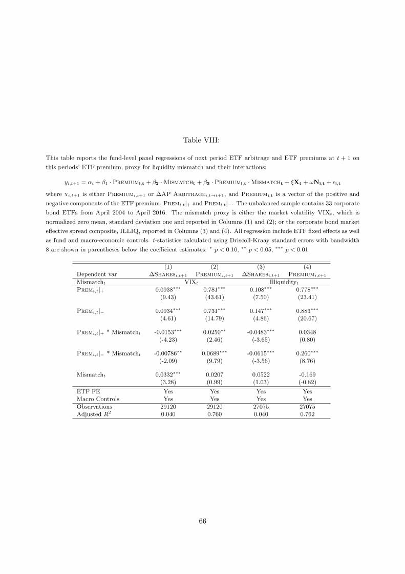
Table VIII:

This table reports the fund-level panel regressions of next period ETF arbitrage and ETF premiums at t + 1 on

this periods’ ETF premium, proxy for liquidity mismatch and their interactions:

yi,t+1 = αi + β1 · Premiumi,t + β2 ·Mismatcht + β3 · Premiumi,t ·Mismatcht + ξXt + ωNi,t + εi,t

where yi,t+1 is either Premiumi,t+1 or ∆AP Arbitragei,t→t+1, and Premiumi,t is a vector of the positive and

negative components of the ETF premium, Premi,t|+ and Premi,t|−. The unbalanced sample contains 33 corporate

bond ETFs from April 2004 to April 2016. The mismatch proxy is either the market volatility VIXt, which is

normalized zero mean, standard deviation one and reported in Columns (1) and (2); or the corporate bond market

effective spread composite, ILLIQt reported in Columns (3) and (4). All regression include ETF fixed effects as well

as fund and macro-economic controls. t-statistics calculated using Driscoll-Kraay standard errors with bandwidth

8 are shown in parentheses below the coefficient estimates: ∗ p < 0.10, ∗∗ p < 0.05, ∗∗∗ p < 0.01.

(1) (2) (3) (4)Dependent var ∆Sharesi,t+1 Premiumi,t+1 ∆Sharesi,t+1 Premiumi,t+1

Mismatcht VIXt Illiquidityt

Premi,t|+ 0.0938∗∗∗ 0.781∗∗∗ 0.108∗∗∗ 0.778∗∗∗

(9.43) (43.61) (7.50) (23.41)

Premi,t|− 0.0934∗∗∗ 0.731∗∗∗ 0.147∗∗∗ 0.883∗∗∗

(4.61) (14.79) (4.86) (20.67)

Premi,t|+ * Mismatcht -0.0153∗∗∗ 0.0250∗∗ -0.0483∗∗∗ 0.0348(-4.23) (2.46) (-3.65) (0.80)

Premi,t|− * Mismatcht -0.00786∗∗ 0.0689∗∗∗ -0.0615∗∗∗ 0.260∗∗∗

(-2.09) (9.79) (-3.56) (8.76)

Mismatcht 0.0332∗∗∗ 0.0207 0.0522 -0.169(3.28) (0.99) (1.03) (-0.82)

ETF FE Yes Yes Yes YesMacro Controls Yes Yes Yes Yes

Observations 29120 29120 27075 27075Adjusted R2 0.040 0.760 0.040 0.762

66

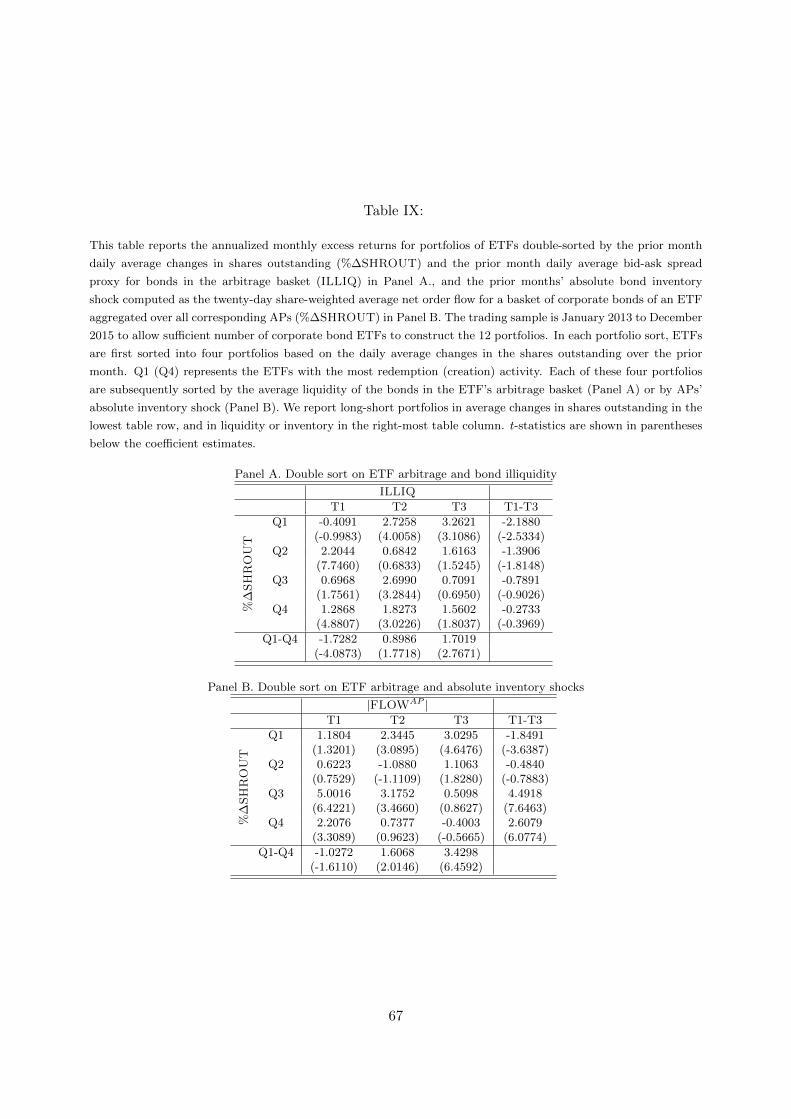
Table IX:

This table reports the annualized monthly excess returns for portfolios of ETFs double-sorted by the prior month

daily average changes in shares outstanding (%∆SHROUT) and the prior month daily average bid-ask spread

proxy for bonds in the arbitrage basket (ILLIQ) in Panel A., and the prior months’ absolute bond inventory

shock computed as the twenty-day share-weighted average net order flow for a basket of corporate bonds of an ETF

aggregated over all corresponding APs (%∆SHROUT) in Panel B. The trading sample is January 2013 to December

2015 to allow sufficient number of corporate bond ETFs to construct the 12 portfolios. In each portfolio sort, ETFs

are first sorted into four portfolios based on the daily average changes in the shares outstanding over the prior

month. Q1 (Q4) represents the ETFs with the most redemption (creation) activity. Each of these four portfolios

are subsequently sorted by the average liquidity of the bonds in the ETF’s arbitrage basket (Panel A) or by APs’

absolute inventory shock (Panel B). We report long-short portfolios in average changes in shares outstanding in the

lowest table row, and in liquidity or inventory in the right-most table column. t-statistics are shown in parentheses

below the coefficient estimates.

Panel A. Double sort on ETF arbitrage and bond illiquidity

ILLIQ

T1 T2 T3 T1-T3

%∆SHROUT

Q1 -0.4091 2.7258 3.2621 -2.1880(-0.9983) (4.0058) (3.1086) (-2.5334)

Q2 2.2044 0.6842 1.6163 -1.3906(7.7460) (0.6833) (1.5245) (-1.8148)

Q3 0.6968 2.6990 0.7091 -0.7891(1.7561) (3.2844) (0.6950) (-0.9026)

Q4 1.2868 1.8273 1.5602 -0.2733(4.8807) (3.0226) (1.8037) (-0.3969)

Q1-Q4 -1.7282 0.8986 1.7019(-4.0873) (1.7718) (2.7671)

Panel B. Double sort on ETF arbitrage and absolute inventory shocks

|FLOWAP |T1 T2 T3 T1-T3

%∆SHROUT

Q1 1.1804 2.3445 3.0295 -1.8491(1.3201) (3.0895) (4.6476) (-3.6387)

Q2 0.6223 -1.0880 1.1063 -0.4840(0.7529) (-1.1109) (1.8280) (-0.7883)

Q3 5.0016 3.1752 0.5098 4.4918(6.4221) (3.4660) (0.8627) (7.6463)

Q4 2.2076 0.7377 -0.4003 2.6079(3.3089) (0.9623) (-0.5665) (6.0774)

Q1-Q4 -1.0272 1.6068 3.4298(-1.6110) (2.0146) (6.4592)

67

Table X:

This table reports the bond-level panel regressions at the monthly frequency of corporate bond excess returns on

the share of bond outstanding held by ETFs and measures of AP arbitrage activity:

XRj,t→t+1 = αj + λETFHeldj,t + βAPActivityj,t + ξXt + ωNj,t + εj,t

The unbalanced sample contains all corporate bonds satisfying index inclusion criteria for each index tracked by the

corporate bond ETF from January 2011 to September 2015. ETFHeldj,t is the percent of amount outstanding (in

par dollars) held by all the corporate bond ETFs in the sample. There are two measures of AP arbitrage activity:

C/R Intensityj,t captures the intensity of AP arbitrage and is equal to the daily standard deviation of ETF

shares outstanding scaled by the level for each month t, and finally normalized to mean zero, standard deviation

one; Creationj,t and Redemptionj,t is the weighted average of total ETF creations and redemptions as a percent

of share outstanding over all ETF holding bond j over month t. BasketCR (BasketRD) is equal to the fraction

of trading dates for which a bond is in the creation (redemption) arbitrage basket. Premiumj,t is the weighted

average of daily ETF premium calculated over ETFs holding bond j; σ(Premium)j,t is the standard deviation

of daily ETF premium calculated over ETFs holding bond j. The dependent variable in Columns (1) to (6) is

XRj,t→t+1 equal to the corporate bond return is in excess of the one-month Treasury bond return and is reported

in basis points; the dependent variable in Column (7) to (8) is the Y spdj,t equal to the yield spread (in basis points)

above the one-month Treasury bond yield. All regressions include bond fixed effects as well as all macroeconomic

and time-varying bond-level controls at time t. t-statistics calculated using double-clustered standard errors on

month-year and bond CUSIP are shown in parentheses: ∗ p < 0.10, ∗∗ p < 0.05, ∗∗∗ p < 0.01.

(1) (2) (3) (4) (5) (6) (7)

Dependent variable XRj,t→t+1 Y spdj,t

ETFHeldj,t -11.03∗∗ -12.32∗∗ -10.02∗ -9.587∗ -13.27∗∗ -8.285∗∗∗ 5.296∗∗

(-2.17) (-2.27) (-1.98) (-1.87) (-2.02) (-3.87) (2.45)

C/R Intensityj,t -19.32∗∗

(-2.07)

Creationj,t -4.937∗∗ -4.985∗ -7.476∗∗ -0.778 -1.175∗∗

(-2.00) (-1.90) (-2.29) (-1.47) (-2.13)

Redemptionj,t -6.853∗∗ -9.071∗∗∗ -10.61∗∗∗ -0.773 -0.575(-2.19) (-2.94) (-3.06) (-1.21) (-0.98)

Creationj,t ×BasketCRj,t -0.0140 -0.0615 0.449 1.052

(-0.01) (-0.04) (0.98) (1.66)

Redemptionj,t ×BasketRDj,t 4.454∗∗ 6.225∗∗ 1.364∗∗ 1.285∗∗

(2.09) (2.54) (2.35) (2.36)

BasketCRj,t -4.162 -8.368 -0.203 -2.661

(-0.41) (-0.68) (-0.08) (-0.81)

BasketRDj,t -13.42∗ -21.13∗ -17.74∗∗∗ -14.83∗∗∗

(-1.68) (-1.93) (-5.06) (-4.67)

CUSIP FE Yes Yes Yes Yes Yes Yes YesMacro Controls Yes Yes Yes Yes Yes Yes YesETF Premium Controls No Yes Yes Yes Yes Yes YesMutual Fund Controls No No No No Yes No Yes

Observations 283659 283659 242922 242922 117757 237796 117373Adjusted R2 0.021 0.037 0.053 0.055 0.060 0.844 0.846

68

Table XI:

This table reports the portfolio-level panel regressions at the daily frequency of corporate bond illiquidity on the

positive and negative components of ETF premiums and changes in ETF shares outstanding:

log

(PC1k,t+1

PC1k,t

)= αi + ξt +

∑j∈+,−

∆SHROUTETFi,t |j +

∑j∈+,−

Premi,t−1|j

+∑

j∈+,−

∑k∈+,−

(∆SHROUTETF

i,t |j × Premi,t−1|k)

+ εi,t

where Premi,t|+ and Premi,t|− are the positive and negative components of the ETF premium, and

SHROUTETFi,t |+ and SHROUTETF

i,t |− are ETF creations and redemptions. The dependent variable is the log

difference between the first principal component of three liquidity proxies from t to t+ 1, log(

PC1k,t+1

PC1k,t

). PC1k,t is

the first principal component of three liquidity proxies: effective spread, Amihud price impact and bond turnover.

This table consider four portfolios k constructed for each ETF: the creation basket (Column (1)), the redemption

basket (Column (2)), the entire ETF portfolio holdings (Column (3)), and the ETF portfolio holdings without

bonds appearing in the creation or redemption basket (Column (4)). Total marginal effects following a one stan-

dard deviation shock are reported in the lower part of the table for each possible ETF premium and arbitrage

state; σ(Basketk) is the standard deviation of PC1k,t in the sample for each basket k. All regression include ETF

and date fixed effects. t-statistics calculated using Driscoll-Kraay standard errors with bandwidth 8 are shown in

parentheses below the coefficient estimates: ∗ p < 0.10, ∗∗ p < 0.05, ∗∗∗ p < 0.01.

(1) (2) (3) (4)Portfolio k

Creation Redemption ETF PortfolioETF Portfolio

(No arb. bonds)

∆SHROUTETFi,t |+ × Premi,t−1|+ -8.596∗∗∗ -1.962 -4.370∗∗ -2.638

(-3.30) (-0.82) (-2.33) (-1.09)

∆SHROUTETFi,t |+ × Premi,t−1|− -39.30 45.30 20.31 27.30

(-1.09) (0.76) (0.91) (1.02)

∆SHROUTETFi,t |− × Premi,t−1|+ 11.12 -14.99∗ 5.313 -0.510

(1.17) (-1.87) (1.24) (-0.09)

∆SHROUTETFi,t |− × Premi,t−1|− -7.943 -10.51∗∗ -5.171 0.179

(-1.02) (-2.13) (-1.23) (0.04)

∆SHROUTETFi,t |+ 3.102∗ 1.242 -1.715∗∗ -2.953∗∗∗

(1.95) (0.85) (-1.98) (-2.62)

∆SHROUTETFi,t |− -1.943 1.588 0.469 2.625∗

(-0.95) (0.90) (0.44) (1.95)

PREMi,t−1|+ -0.171 1.389∗ 1.505∗∗ -4.590∗∗

(-0.16) (1.77) (2.17) (-2.15)

PREMi,t−1|− 1.389 1.778 2.706∗∗ 5.512(0.83) (1.30) (2.26) (1.18)

Total marginal effect following 1sd shock

∆SHROUTETF |+, Prem|+ -5.072 0.0982 -3.489 -6.858∆SHROUTETF |+, Prem|− 5.723 -2.892 -2.171 -2.836∆SHROUTETF |−, Prem|+ -0.690 2.523 -0.413 -5.033∆SHROUTETF |−, Prem|− -1.426 -5.251 -1.877 -0.667σ (Basketk) 44.66 36.48 29.36 31.66

ETF FE Yes Yes Yes YesDate FE Yes Yes Yes Yes

Observations 22307 22497 19993 11477Adjusted R2 0.376 0.471 0.684 0.684

69

Table XII:

This table reports bond-level panel regressions at the weekly frequency of one- and multiweek returns on AP

arbitrage, as proxied by percentage changes in ETF shares outstanding, and controls:

Rj,ti→tj = αj + γt + β1(

%CreationETFt

)+ β2

(%RedemptionETF

t

)+ ωNj,t + εj,t

The unbalanced sample contains all corporate bonds held by corporate bond ETF from January 2011 to Septem-

ber 2015. Corporate bond returns are calculated using secondary market transaction prices at the end of each

week and are reported in percent. The positive (negative) components of the weekly changes in shares outstand-

ing for ETF creation (redemption) arbitrage activity as a fraction of lagged ETF shares are %CreationETFt

(%RedemptionETFt ). ILLIQj,t is the first principal component extracted from a vector of bond illiquidity mea-

sures: turnover, spread, FHT, zeros and price impact. All regressions include bond and week fixed effects as well

as time-varying bond-level controls at time t, and the lagged dependent value. The lagged dependent variable is

lagged k periods where k is set to have the return horizon end in ti−1. t-statistics calculated using double-clustered

standard errors on week-year and bond CUSIP are shown in parentheses below the coefficient estimates: ∗ p < 0.10,∗∗ p < 0.05, ∗∗∗ p < 0.01.

(1) (2) (3) (4)Dependent variable Rt−1→t Rt−1→t+1 Rt+1→t+2 Rt+1→t+4

%CreationETFt 2.395∗∗∗ 1.946∗∗∗ 0.336 0.141

(8.75) (4.31) (0.84) (0.25)

%RedemptionETFt -1.948∗∗∗ -1.759∗∗∗ 0.958∗∗∗ 1.358∗∗∗

(-4.52) (-3.50) (3.30) (2.97)

ILLIQj,t 0.0545 0.392 0.0566 0.364(0.21) (1.07) (0.25) (0.99)

AP Inventoryj,t−1 3.435∗∗∗ -9.086∗∗∗ 1.372∗∗ -13.39∗∗∗

(2.97) (-7.72) (1.99) (-8.10)

AMTOUTj,t 4.769∗∗∗ 7.136∗∗∗ 2.836∗∗ 7.506∗∗

(3.41) (3.27) (2.13) (2.45)

RTGj,t 1.762∗∗∗ 3.731∗∗∗ 1.778∗∗∗ 5.329∗∗∗

(4.45) (6.09) (4.82) (6.56)

1{On the run}j,t -0.221 -0.784 -0.413 -2.427∗∗

(-0.43) (-0.97) (-0.85) (-2.35)

AGEj,t 2541.0∗ 1133.3 -2582.4 3963.8∗∗

(1.72) (0.73) (-1.60) (2.09)

Lagged Dep Var Yes Yes Yes YesTime FE Yes Yes Yes YesCUSIP FE Yes Yes Yes Yes

Observations 723401 679466 671038 638666Adjusted R2 0.187 0.242 0.143 0.253

70