etd.lib.metu.edu.tr of the thesis: ROBUST TRANSMISSION OF 3D MODELS submitted by MEHMET OGUZ B˘...

ROBUST TRANSMISSION OF 3D MODELS

A THESIS SUBMITTED TOTHE GRADUATE SCHOOL OF NATURAL AND APPLIED SCIENCES

OFMIDDLE EAST TECHNICAL UNIVERSITY

BY

MEHMET OGUZ BICI

IN PARTIAL FULFILLMENT OF THE REQUIREMENTSFOR

THE DEGREE OF DOCTOR OF PHILOSOPHYIN

ELECTRICAL AND ELECTRONICS ENGINEERING

NOVEMBER 2010

Approval of the thesis:


submitted byMEHMET O GUZ BIC I in partial fulfillment of the requirements for the degreeof Doctor of Philosophy in Electrical and Electronics Engineering Department, MiddleEast Technical Universityby,

Prof. Dr. CananOzgenDean, Graduate School ofNatural and Applied Sciences

Prof. Dr. Ismet ErkmenHead of Department,Electrical and Electronics Engineering

Prof. Dr. Gozde Bozdagı AkarSupervisor,Electrical and Electronics Engineering Dept., METU

Examining Committee Members:

Prof. Dr. Aydın AlatanElectrical and Electronics Engineering Dept., METU

Prof. Dr. Gozde Bozdagı AkarElectrical and Electronics Engineering Dept., METU

Prof. Dr. A. Enis CetinElectrical and Electronics Engineering Dept., Bilkent University

Assoc. Prof. Dr. Ugur GudukbayComputer Engineering Dept., Bilkent University

Assist. Prof.Ilkay UlusoyElectrical and Electronics Engineering Dept., METU

Date:

I hereby declare that all information in this document has been obtained and presentedin accordance with academic rules and ethical conduct. I also declare that, as requiredby these rules and conduct, I have fully cited and referencedall material and results thatare not original to this work.

Name, Last Name: MEHMET OGUZ BICI

Signature :

iii

ABSTRACT


Bici, Mehmet Oguz

Ph.D., Department of Electrical and Electronics Engineering

Supervisor : Prof. Dr. Gozde Bozdagı Akar

November 2010, 141 pages

In this thesis, robust transmission of 3D models represented by static or time consistent an-

imated meshes is studied from the aspects of scalable coding, multiple description coding

(MDC) and error resilient coding. First, three methods for MDC of static meshes are pro-

posed which are based on multiple description scalar quantization, partitioning wavelet trees

and optimal protection of scalable bitstream by forward error correction (FEC) respectively.

For each method, optimizations and tools to decrease complexity are presented. The FEC

based MDC method is also extended as a method for packet loss resilient transmission fol-

lowed by in-depth analysis of performance comparison with state of the art techniques, which

pointed significant improvement. Next, three methods for MDC of animated meshes are pro-

posed which are based on layer duplication and partitioningof the set of vertices of a scalable

coded animated mesh by spatial or temporal subsampling where each set is encoded sep-

arately to generate independently decodable bitstreams. The proposed MDC methods can

achieve varying redundancy allocations by including a number of encoded spatial or tem-

poral layers from the other description. The algorithms areevaluated with redundancy-rate-

distortion curves and per-frame reconstruction analysis.Then for layered predictive compres-

sion of animated meshes, three novel prediction structuresare proposed and integrated into

iv

a state of the art layered predictive coder. The proposed structures are based on weighted

spatial/temporal prediction and angular relations of triangles between current and previous

frames. The experimental results show that compared to state of the art scalable predictive

coder, up to 30% bitrate reductions can be achieved with the combination of proposed pre-

diction schemes depending on the content and quantization level. Finally, optimal quality

scalability support is proposed for the state of the art scalable predictive animated mesh cod-

ing structure, which only supports resolution scalability. Two methods based on arranging

the bitplane order with respect to encoding or decoding order are proposed together with a

novel trellis based optimization framework. Possible simplifications are provided to achieve

tradeoff between compression performance and complexity. Experimental results show that

the optimization framework achieves quality scalability with significantly better compression

performance than state of the art without optimization.

Keywords: 3D mesh, multiple description coding, error resilient coding, predictive coding,

scalable coding

v

OZ

3B MODELLERIN DAYANIKLI ILETIM I

Bici, Mehmet Oguz

Doktora, Elektrik ve Elektronik Muhendislig Bolumu

Tez Yoneticisi : Prof. Dr. Gozde Bozdagı Akar

Kasım 2010, 141 sayfa

Bu tezde statik veya zaman tutarlı hareketli tel orguler ile temsil edilen 3B modellerin dayanıklı

iletimi olceklenebilir kodlama, coklu anlatım (CA) kodlama ve hataya dayanıklı kodlama

yonlerinden incelenmistir. Ilk olarak, statik tel orgulerin CA kodlanması icin coklu an-

latım skaler nicemleme, dalgacık agacların ayrılması veolceklenebilir bitkatarının ileri hata

koruma (IHK) ile en iyi korunmasına dayalı uc metot onerilmistir. Her metot icin en iy-

ilemeler ve karmasıklıgı azaltıcı araclar sunulmustur. IHK kullanan CA kodlama metodu

ayrıca paket kayıplarına dayanıklı iletim icin bir metot olarak genisletilmis ve derinleme-

sine analizın ardından en ileri teknoloji teknikler ile performansı karsılastırılmıs, onemli

iyilesmeler gozlenmistir. Sonra, hareketli tel orgulerin CA kodlanması icin katman kopy-

alama ve olceklenebilir kodlanmıs tel orgunun dugum kumesinin uzamsal veya zamansal alt

orneklenmesiyle boluntulenmesine dayalı uc metot ¨onerilmistir. Her kume bagımsız olarak

kodcozulebilir bitkatarı uretmek uzere ayrı olarak kodlanmıstır.Onerilen CA kodlama metot-

ları diger kumeden belli sayıda uzamsal ya da zamansal katmanları icererek degisken artıklık

tahsis edebilmektedir.Onerilen metotlar artıklık-hız-bozulum egrileri ve cerceve basına geri

catılım analizi ile degerlendirilmistir. Daha sonra, hareketli tel orgulerin katmanlı ve ongorucu

sıkıstırılması icin uc ozgun ongoru yapısı onerilmis ve son teknoloji katmanlı ongorucu bir

vi

kodlayıcıya eklenmistir.Onerilen yapılar agırlıklandırılmıs uzamsal/zamansal ongoru ve su

anki ve onceki cerceve arasındaki ucgenlerin acısaliliskilerine dayanmaktadır. Deneylerde

son teknoloji olceklenebilir ongorucu kodlama ile karsılastırıldıgında, icerik ve nicemleme se-

viyesine baglı olarak onerilen yapıların kombinasyonları ile 30%’a varan bit hızı kazancı elde

edilebildigi gorulmustur. Son olarak, son teknoloji olceklenebilir ongorucu hareketli tel orgu

kodlama yapısına en iyi kalite olceklenebilme destegi ¨onerilmistir; ki o sadece cozunurluk

olceklenebilirligi desteklemektedir. Bit duzlemi sıralamasının kodlama veya kodcozme sırasına

gore ayarlanmasına dayalı iki metot onerilmistir. Metotlar ozgun olarak kafese dayalı en iy-

ileme cercevesi kullanmaktadır. Sıkıstırma performansı ve karmasıklık arası odunlesim elde

etmek icin olası basitlestirmeler sunulmustur. Deneysel sonuclar en iyileme cercevesinin

en iyilemesiz son teknolojiden onemli boyutta daha iyi sıkıstırma performansı elde ettigini

gostermistir.

Anahtar Kelimeler: 3B tel orgu, coklu anlatım kodlama, hataya dayanıklı kodlama, ongorucu

kodlama, olceklenebilir kodlama

vii

To my wife

viii

ACKNOWLEDGMENTS

I would like to express my sincere and deepest gratitude to mysupervisor Gozde Bozdagı

Akar for her supervision, guidance and encouragements. I deeply appreciate her support in

every part of my PhD. I would also like to thank Prof. Aydın Alatan and Assoc. Prof. Ugur

Gudukbay for their valuable comments and feedbacks during my thesis progress meetings.

I would like to acknowledge the following researchers for their cooperation and contributions

to my thesis. I would like to thank Anıl Aksay who always shared his knowledge and expe-

rience with me. I would like to acknowledge Andrey Norkin forour efficient collaborative

works. I would like to thank Nikolce Stefanoski for hosting me, for providing his dynamic

mesh coder software and for the very helpful discussions. I would like to acknowledge Kıvanc

Kose for our useful discussions about meshes.

I would like to acknowledge all my friends in Multimedia Research Group at METU for

creating a very enjoyable lab environment in the past years.Thank you Cagdas Bilen, Cevahir

Cıgla, Erman Okman, Anıl Aksay,Ozgu Alay, Alper Koz,Ozlem Pasin, Yusuf Bediz, Eren

Gurses, Ahmet Saracoglu, Engin Tola, BirantOrten, BurakOzkalaycı, EvrenImre, Yusuf

Bayraktaroglu, Serdar Gedik, Murat Deniz Aykın, Bertan G¨unyel, Emrah Bala, Elif Vural,

Yoldas Ataseven, Oytun Akman, Cem Vedat Isık, Berkan Solmaz, Done Bugdaycı, Murat

Demirtas and others.

I would like to dedicate this thesis to my dear wife,Ipek Bici, who always supported me with

her endless love in every part of my life. Finally, I would like thank all my family for their

love and support.

This thesis is partially supported by European Commission within FP6 under Grant 511568

with the acronym 3DTV, within FP7 under Grant 216503 with theacronym MOBILE3DTV

and The Scientific and Technological Research Council of Turkey (TUBITAK) under National

Scholarship Programme for PhD Students.

The chicken character was created by Andrew Glassner, Tom McClure, Scott Benza, and

ix

Mark Van Langeveld. This short sequence of connectivity andvertex position data is dis-

tributed solely for the purpose of comparison of geometry compression techniques.

x

TABLE OF CONTENTS

ABSTRACT . . . . . . . . . . . . . . . . . . . . . . . . . . . . . . . . . . . . . . . . iv

OZ . . . . . . . . . . . . . . . . . . . . . . . . . . . . . . . . . . . . . . . . . . . . . vi

ACKNOWLEDGMENTS . . . . . . . . . . . . . . . . . . . . . . . . . . . . . . . . . ix

TABLE OF CONTENTS . . . . . . . . . . . . . . . . . . . . . . . . . . . . . . . . . xi

LIST OF TABLES . . . . . . . . . . . . . . . . . . . . . . . . . . . . . . . . . . . . xv

LIST OF FIGURES . . . . . . . . . . . . . . . . . . . . . . . . . . . . . . . . . . . . xvii

LIST OF ABBREVIATIONS . . . . . . . . . . . . . . . . . . . . . . . . . . . . . . . xxii

CHAPTERS

1 INTRODUCTION . . . . . . . . . . . . . . . . . . . . . . . . . . . . . . . 1

1.1 Scope and Outline of the Thesis . . . . . . . . . . . . . . . . . . . . 3

2 BACKGROUND . . . . . . . . . . . . . . . . . . . . . . . . . . . . . . . . 4

2.1 3D Mesh Data . . . . . . . . . . . . . . . . . . . . . . . . . . . . . 4

2.2 Error Resilient Coding . . . . . . . . . . . . . . . . . . . . . . . . . 5

2.2.1 Multiple Description Coding . . . . . . . . . . . . . . . . 6

2.2.1.1 Redundancy Allocation . . . . . . . . . . . . 8

2.2.1.2 Mismatch Control . . . . . . . . . . . . . . . 8

2.2.2 Packet Loss Resilient Streaming . . . . . . . . . . . . . . 9

2.3 Scalable Coding . . . . . . . . . . . . . . . . . . . . . . . . . . . . 9

2.4 Forward Error Correction . . . . . . . . . . . . . . . . . . . . . . . 10

3 3D MESH CODING . . . . . . . . . . . . . . . . . . . . . . . . . . . . . . 11

3.1 Literature Review on Static 3D Mesh Coding . . . . . . . . . . . .. 11

3.1.1 Wavelet Based Scalable Static 3D Mesh Coding and PGC 12

3.1.2 Compressed Progressive Meshes (CPM) . . . . . . . . . . 13

xi

3.2 Literature Review on Animated 3D Mesh Coding . . . . . . . . . .14

3.2.1 Scalable Predictive Coding (SPC) - MPEG-4 FAMC . . . 18

3.3 3D Mesh Distortion Metrics . . . . . . . . . . . . . . . . . . . . . . 23

3.3.1 Static 3D Mesh Distortion Metrics . . . . . . . . . . . . . 23

3.3.2 Animated 3D Mesh Distortion Metrics . . . . . . . . . . . 24

4 MULTIPLE DESCRIPTION CODING OF STATIC 3D MESHES . . . . . . 25

4.1 Introduction - Literature Review . . . . . . . . . . . . . . . . . . .25

4.2 Proposed MDSQ . . . . . . . . . . . . . . . . . . . . . . . . . . . . 26

4.3 Proposed Tree Partitioning . . . . . . . . . . . . . . . . . . . . . . 31

4.4 Proposed FEC Based Approach for MDC . . . . . . . . . . . . . . . 40

4.4.1 Problem Definition and Proposed Solution . . . . . . . . . 40

4.4.2 MDC Experimental Results . . . . . . . . . . . . . . . . 42

4.5 Extension of MD-FEC to Packet Loss Resilient Coding . . . .. . . 43

4.5.1 Packet Loss Resilient Coding Based on CPM . . . . . . . 44

4.5.2 Proposed Modifications for CPM based Loss Resilient Cod-ing . . . . . . . . . . . . . . . . . . . . . . . . . . . . . . 45

4.5.3 Distortion Metric and Simplifications in Calculations . . . 46

4.5.4 Channel Model . . . . . . . . . . . . . . . . . . . . . . . 46

4.5.5 Experimental Results . . . . . . . . . . . . . . . . . . . . 47

4.5.5.1 Proposed kStep for CPM Based Methods . . . 48

4.5.5.2 Comparison of CPM Based Methods . . . . . 49

4.5.5.3 Performance of D-R Curve Modeling for PGCBased Methods . . . . . . . . . . . . . . . . 50

4.5.5.4 Comparison of CPM and PGC Based Methods 50

4.5.5.5 Mismatch Scenario . . . . . . . . . . . . . . 53

4.5.5.6 Complexity Comparison . . . . . . . . . . . . 54

4.5.5.7 Visual Comparison of CPM and PGC BasedMethods . . . . . . . . . . . . . . . . . . . . 55

4.6 Conclusions . . . . . . . . . . . . . . . . . . . . . . . . . . . . . . 55

5 MULTIPLE DESCRIPTION CODING OF ANIMATED MESHES . . . . . . 60

5.1 Introduction . . . . . . . . . . . . . . . . . . . . . . . . . . . . . . 60

xii

5.2 Reference Dynamic Mesh Coder . . . . . . . . . . . . . . . . . . . 61

5.3 Proposed MDC Methods . . . . . . . . . . . . . . . . . . . . . . . 61

5.3.1 Vertex Partitioning Based MDC . . . . . . . . . . . . . . 62

5.3.1.1 MD Encoder . . . . . . . . . . . . . . . . . . 62

5.3.1.2 MD Side Decoder . . . . . . . . . . . . . . . 64

5.3.1.3 MD Central Decoder . . . . . . . . . . . . . 65

5.3.2 Temporal Subsampling Based MDC . . . . . . . . . . . . 66

5.3.2.1 MD Encoder . . . . . . . . . . . . . . . . . . 66

5.3.2.2 MD Side Decoder . . . . . . . . . . . . . . . 67


5.3.3 Layer Duplication Based MDC . . . . . . . . . . . . . . . 68

5.3.3.1 MD Encoder . . . . . . . . . . . . . . . . . . 68

5.3.3.2 MD Side Decoder . . . . . . . . . . . . . . . 70


5.3.4 Comments on the Mismatch . . . . . . . . . . . . . . . . 70

5.3.5 Further Possible Improvements on Error Concealment .. 71

5.4 Results . . . . . . . . . . . . . . . . . . . . . . . . . . . . . . . . . 71

5.4.1 Vertex Partitioning . . . . . . . . . . . . . . . . . . . . . 73

5.4.2 Temporal Subsampling . . . . . . . . . . . . . . . . . . . 75

5.4.3 Layer Duplication . . . . . . . . . . . . . . . . . . . . . . 75

5.4.4 Comparison . . . . . . . . . . . . . . . . . . . . . . . . . 76

5.4.5 Per Frame Analysis . . . . . . . . . . . . . . . . . . . . . 79

5.5 Conclusions and Future Work . . . . . . . . . . . . . . . . . . . . . 85

6 IMPROVED PREDICTION METHODS FOR SCALABLE PREDICTIVEANIMATED MESH COMPRESSION . . . . . . . . . . . . . . . . . . . . . 86

6.1 Prediction Structures . . . . . . . . . . . . . . . . . . . . . . . . . . 86

6.1.1 Proposed Weighted Spatial Prediction . . . . . . . . . . . 88

6.1.2 Proposed Weighted Temporal Prediction . . . . . . . . . . 89

6.1.3 Proposed Angle Based Predictor . . . . . . . . . . . . . . 90

6.2 Experimental Results . . . . . . . . . . . . . . . . . . . . . . . . . 95

6.3 Conclusion . . . . . . . . . . . . . . . . . . . . . . . . . . . . . . . 104

xiii

7 OPTIMAL QUALITY SCALABLE CODING OF ANIMATED MESHES . . 105

7.1 Introduction . . . . . . . . . . . . . . . . . . . . . . . . . . . . . . 105

7.2 Proposed Quality Scalable Coding: Decoding Order Based. . . . . 106

7.2.1 Optimization . . . . . . . . . . . . . . . . . . . . . . . . 107

7.2.2 Rate, Distortion and Path Metrics . . . . . . . . . . . . . 112

7.2.3 Algorithmic Simplifications . . . . . . . . . . . . . . . . 112

7.3 Proposed Quality Scalable Coding: Encoding Order Based. . . . . 113

7.3.1 Rate, Distortion and Path Metrics . . . . . . . . . . . . . 114

7.4 Experimental Results . . . . . . . . . . . . . . . . . . . . . . . . . 116

7.4.1 Slope Based Optimization . . . . . . . . . . . . . . . . . 116

7.4.2 Simple Encoding Parameters - Full Trellis . . . . . . . . . 117

7.4.3 Effect of Rate Intervals . . . . . . . . . . . . . . . . . . . 118

7.4.4 Comparison of DOB and EOB . . . . . . . . . . . . . . . 120

7.4.5 Complexity Considerations . . . . . . . . . . . . . . . . . 122

7.4.6 Visual Comparisons . . . . . . . . . . . . . . . . . . . . . 123

7.5 Conclusion . . . . . . . . . . . . . . . . . . . . . . . . . . . . . . . 127

8 CONCLUSION . . . . . . . . . . . . . . . . . . . . . . . . . . . . . . . . . 128

REFERENCES . . . . . . . . . . . . . . . . . . . . . . . . . . . . . . . . . . . . . . 131

CURRICULUM VITAE . . . . . . . . . . . . . . . . . . . . . . . . . . . . . . . . . 138

xiv

LIST OF TABLES

TABLES

Table 4.1 File Sizes for differentRwhenk = 1 . . . . . . . . . . . . . . . . . . . . . 28

Table 4.2 RelativeL2 errors for the case in Table 4.1 . . . . . . . . . . . . . . . . . . 29

Table 4.3 File Sizes for differentk whenR= 6 . . . . . . . . . . . . . . . . . . . . . 31

Table 4.4 RelativeL2 errors for the case in Table 4.3 . . . . . . . . . . . . . . . . . . 31

Table 4.5 An example FEC assignment on an embedded bitstream. There areN = 5

packets each composed ofL = 4 symbols. Therefore there are 4 source segments,

Si , i = 1, 2, 3, 4 each of which containsmi data symbols andfi FEC symbols

wheremi + fi = N. In this examplem1 = 2, f1 = 3,m2 = 3, f2 = 2,m3 = 3, f3 =

2,m4 = 4, f4 = 1. Earlier parts of the bitstream are assigned more FEC symbols

since they contribute more to overall quality. . . . . . . . . . . .. . . . . . . . . 41

Table 4.6 An example CPM output withLM + 1 = 3 layers. Pi denotes Packeti

generated horizontally while FEC is applied vertically. Inthis simple example

N = 6, k0 = 2, k1 = 3 andk2 = 4. . . . . . . . . . . . . . . . . . . . . . . . . . . 44

Table 4.7 Simulated distortion results of the first scenariofor variousPLR values. The

distortion metric is relativeL2 error in units of 10−4. . . . . . . . . . . . . . . . . 51

Table 4.8 Optimization times of different methods. Each method is optimized for

PLR = 4% . . . . . . . . . . . . . . . . . . . . . . . . . . . . . . . . . . . . . . 55

Table 5.1 The test sequences . . . . . . . . . . . . . . . . . . . . . . . . . . .. . . . 72

Table 6.1 The test sequences . . . . . . . . . . . . . . . . . . . . . . . . . . .. . . . 95

Table 6.2 Bitrate reductions compared to SPC for cowheavy, chicken crossing and

dance sequences . . . . . . . . . . . . . . . . . . . . . . . . . . . . . . . . . . . 100

Table 6.3 Bitrate reductions compared to SPC for horse gallop, face and jump . . . . 101

xv

Table 7.1 Average optimization time during encoding per GOMin minutes. . . . . . . 123

xvi

LIST OF FIGURES

FIGURES

Figure 2.1 Single description and multiple description coding. R0: central or single

description bitrate. D0: central distortion. R1,R2: side bitrates. D1,D2: side

distortions. . . . . . . . . . . . . . . . . . . . . . . . . . . . . . . . . . . . . . . 7

Figure 3.1 Classification of 3D mesh compression methods . . .. . . . . . . . . . . 12

Figure 3.2 Generation of embedded bitstream from PGC coder.The bitstream starts

with compressed coarsest level connectivity (C) as it is the most important part on

which the whole mesh connectivity depends. The next part of the bitstream is a

predetermined number of bit-planes (5 in the figure) of the coarsest level geometry

(G1G2G3G4G5) since wavelet coefficients would have no use without coarsest

level geometry. Remaining part of the bitstream consists ofthe output bitstream

of SPIHT for different quantization levels (S1S2S3..) and after each quantization

level, refinement bit-planes of coarsest level geometry (G6G7..) are inserted for

improved progressivity. . . . . . . . . . . . . . . . . . . . . . . . . . . . . .. . 13

Figure 3.3 Hierarchical temporal prediction structure . . .. . . . . . . . . . . . . . . 20

Figure 3.4 Prediction of a vertex in SPC. The vertex to be predicted is denoted byvcc. . 21

Figure 4.1 Encoder block diagram . . . . . . . . . . . . . . . . . . . . . . .. . . . . 27

Figure 4.2 Decoder block diagram . . . . . . . . . . . . . . . . . . . . . . .. . . . . 28

Figure 4.3 Test data (a)Bunnymodel; (b)Venus headmodel. . . . . . . . . . . . . . 29

Figure 4.4 (a) File Sizes (b) RelativeL2 errors for differentRwhenk = 1 . . . . . . . 30

Figure 4.5 (a) File Sizes (b) RelativeL2 errors for differentk whenR= 6 . . . . . . . 30

Figure 4.6 Reconstructed models for ML(6,1): (a)-(b) Reconstruction from one de-

scription (Side1andSide2) (c) Reconstruction from both of the descriptions (Cen-

tral). . . . . . . . . . . . . . . . . . . . . . . . . . . . . . . . . . . . . . . . . . 30

xvii

Figure 4.7 TM-MDC encoder scheme. . . . . . . . . . . . . . . . . . . . . . .. . . 32

Figure 4.8 Reconstruction of modelBunnyfrom one description among four descrip-

tions for different types of tree grouping. (a) Spatially disperse grouping; PSNR=

50.73 dB. (b) Spatially close grouping, group size is 10; PSNR= 48.51 dB. . . . . 33

Figure 4.9 Comparison between the Weibull model (10 points)and operational D-R

curve (L2) for Bunnymodel. (a) RelativeL2 error; (b) PSNR. . . . . . . . . . . . 35

Figure 4.10 Reconstruction ofBunnymodel from different number of received descrip-

tions. The results are given for bit allocations for different packet loss rates (PLR).

The redundancyρ is given in brackets. (a) RelativeL2 error; (b) PSNR. . . . . . . 36

Figure 4.11 ModelBunnyencoded into 8 descriptions at total 25944 Bytes. Recon-

structed from different number of descriptions. Compared to unprotected SPIHT. . 36

Figure 4.12 The comparison of network performance of the proposed TM-MDC with a

simple MDC scheme and unprotected SPIHT. (a) RelativeL2 error; (b) PSNR. . . 37

Figure 4.13 Reconstruction of theBunnymodel from (a) one description (48.36 dB),

(b) two descriptions (63.60 dB), (c) three descriptions (71.44 dB), (d) four descrip-

tions (74.33 dB). . . . . . . . . . . . . . . . . . . . . . . . . . . . . . . . . . . . 38

Figure 4.14 Reconstruction ofVenus headmodel from (a) one description (53.97 dB),

(b) two descriptions (65.18 dB), (c) three descriptions (72.51 dB), (d) four descrip-

tions (77.08 dB). . . . . . . . . . . . . . . . . . . . . . . . . . . . . . . . . . . . 39

Figure 4.15 Reconstruction from different number of descriptions (PSNR) forBunny

model. (a) RelativeL2 error; (b) PSNR. . . . . . . . . . . . . . . . . . . . . . . . 42

Figure 4.16 The comparison of the MD-FEC with TM-MDC coder from [1]. (a) Rela-

tive L2 error; (b) PSNR. . . . . . . . . . . . . . . . . . . . . . . . . . . . . . . . 43

Figure 4.17 Two state Markov channel model. . . . . . . . . . . . . . .. . . . . . . . 46

Figure 4.18 Effect of k step size on quality: Simulated PSNR vs k step size forBunny

model optimized forPLR = 2%, 4% and 10% and coded at 3.5 bpv. . . . . . . . . 48

Figure 4.19 Effect of k step size on complexity: Optimization time vs k step size for

Bunnymodel optimized forPLR = 4% and coded at 3.5 bpv. . . . . . . . . . . . . 49

Figure 4.20 Comparison of CPM based methods for Bunny model in terms of simulated

distortions for variousPLR’s. . . . . . . . . . . . . . . . . . . . . . . . . . . . . 49

xviii

Figure 4.21 Comparison of using original D-R curve and usingmodeled D-R curve

during optimization forBunnymodel in terms of simulated distortions for various

PLR’s. . . . . . . . . . . . . . . . . . . . . . . . . . . . . . . . . . . . . . . . . . 51

Figure 4.22PLR vs Simulated distortion in PSNR scale forBunnymodel coded at 3.5

bpv. . . . . . . . . . . . . . . . . . . . . . . . . . . . . . . . . . . . . . . . . . . 52

Figure 4.23PLR vs Simulated distortion in PSNR scale forBunnymodel coded at 1.2

bpv. . . . . . . . . . . . . . . . . . . . . . . . . . . . . . . . . . . . . . . . . . . 52

Figure 4.24PLR vs Simulated distortion in PSNR scale forVenus headmodel coded at

4 bpv. . . . . . . . . . . . . . . . . . . . . . . . . . . . . . . . . . . . . . . . . . 53

Figure 4.25Bunnymodel is coded at 3.5 bpv and FEC assignment is optimized with

respect to three differentPLR’s for PGCStankovicandAlRegib kStep= 5 meth-

ods. Performance of the three different assignments for variousPLR’s in terms of

simulated distortion in PSNR scale. . . . . . . . . . . . . . . . . . . . .. . . . . 54

Figure 4.26 Expected reconstructions of theBunnymodel, left column byPGCStankovic

method and right column byAlRegib kStep=5 method. (a)-(b):PLR = 2%, (c)-

(d):PLR = 10%, (e)-(f):PLR = 20%. PSNR values: (a) 72.18 dB (b) 62.44 dB (c)

70.52 dB (d) 61.57 dB (e) 69.09 dB (f) 58.61 dB . . . . . . . . . . . . . .. . . . 56

Figure 4.27 Expected reconstructions of theVenus headmodel, left column byPGC-

Stankovicmethod and right column byAlRegib kStep=5 method. (a)-(b):PLR =

2%, (c)-(d):PLR = 10%, (e)-(f):PLR = 20%. PSNR values: (a) 76.95 dB (b) 67.79

dB (c) 75.04 dB (d) 65.19 dB (e) 74.24 dB (f) 65.19 dB . . . . . . . . .. . . . . 57

Figure 5.1 Temporal subsampling based MDC. The example sequence is decomposed

into three temporal layers and three spatial layers. One spatial layer from the other

description is duplicated. . . . . . . . . . . . . . . . . . . . . . . . . . . .. . . 66

Figure 5.2 Layer duplication based MDC: three layer ordering examples . . . . . . . 69

Figure 5.3 (a)Vertex Partitioning based MDC: RRD curves forvarying number of du-

plicated layers (b) All achievable RRD points and their convex hull . . . . . . . . 74

Figure 5.4 Comparison of mismatch-free and mismatch-allowed vertex partitioning

based MDC . . . . . . . . . . . . . . . . . . . . . . . . . . . . . . . . . . . . . 74

Figure 5.5 Temporal Subsampling based MDC: (a) RRD curves for different predic-

tion methods (b) Zoomed view . . . . . . . . . . . . . . . . . . . . . . . . . . .75

xix

Figure 5.6 Layer Duplication based MDC: All redundancy-side error pairs and the

convex hull . . . . . . . . . . . . . . . . . . . . . . . . . . . . . . . . . . . . . . 76

Figure 5.7 RRD performance comparison of the MDC methods . . .. . . . . . . . . 78

Figure 5.8 PSNR values of side reconstruction of each frame for horse gallop sequence

MD coded at (a) %25 redundancy, (b) %45 redundancy . . . . . . . . .. . . . . 79

Figure 5.9 Central and side reconstructions of frames 1 and 2of horse gallop sequence

MD coded at 25% redundancy . . . . . . . . . . . . . . . . . . . . . . . . . . . . 81

Figure 5.10 Central and side reconstructions of frames 1 and2 of horse gallop sequence


Figure 5.11 Central and side reconstructions of frames 259 and 260 of chicken sequence


Figure 5.12 Visualization of errors between central and side reconstructions for horse-

gallop and chicken crossing MD coded at 25% and 44% redundancy, respectively.

Deviation from red indicates increasing error. . . . . . . . . . .. . . . . . . . . . 84

Figure 6.1 One incident triangle in previously encoded and current frame. Note that

vp,c0 , vp,c

1 , vp,cs andvp,c

cr lie on the same planePp,cs . . . . . . . . . . . . . . . . . . . 91

Figure 6.2 Angle based prediction (a) Angles same (b) Angle differences same (c)

Local displacement betweenvcr andvs same . . . . . . . . . . . . . . . . . . . . 94

Figure 6.3 The compression performance of angle based prediction methods as a func-

tion of multiplicative constant of standard deviation in outlier removal process as

given in the legend. Q=8 bits: . . . . . . . . . . . . . . . . . . . . . . . . . . . 96

Figure 6.4 The compression performance of angle based prediction methods as a func-

tion of multiplicative constant of standard deviation in outlier removal process as

given in the legend. Q=12 bits . . . . . . . . . . . . . . . . . . . . . . . . . . . 96

Figure 6.5 Change in prediction error compared to SPC per frame . . . . . . . . . . . 97

Figure 6.6 Percentage bitrate reduction compared to SPC perframe . . . . . . . . . . 98

Figure 6.7 RD comparison of the SPC and best performing proposed method for each

quantization level. . . . . . . . . . . . . . . . . . . . . . . . . . . . . . . . . .. 103

Figure 7.1 Illustration of different fixed bitplane orderings on an example case . . . . 107

Figure 7.2 Rate-distortion curves of fixed bitplane ordering methods. . . . . . . . . . 108

xx

Figure 7.3 Illustration of first branches of the trellis structure used in optimization (a)

Initial state (b) First branches (c) Some of the next possible branches (d) Elimina-

tion of paths when two paths end up at the same state (same RD point) . . . . . . 110

Figure 7.4 Comparison of slope based optimizations with fixed ordering policies . . . 117

Figure 7.5 Comparison of full trellis and slope based optimization for simple coding

parameters . . . . . . . . . . . . . . . . . . . . . . . . . . . . . . . . . . . . . . 118

Figure 7.6 Comparison of different RInt and MaxP parameters for the rate interval

based optimization method. . . . . . . . . . . . . . . . . . . . . . . . . . . .. . 119

Figure 7.7 Comparison of best fixed ordering policies, slopebased and rate interval

based optimizations. . . . . . . . . . . . . . . . . . . . . . . . . . . . . . . . .. 119

Figure 7.8 Comparison of proposed DOB and EOB methods for cowheavy model. . . 120

Figure 7.9 Comparison of proposed DOB and EOB methods for chicken crossing model.121

Figure 7.10 Comparison of proposed DOB and EOB methods for face model. . . . . . 121

Figure 7.11 Comparison of visual reconstructions of frames4,6,7,8 for several methods

decoded at 8 bpvf. . . . . . . . . . . . . . . . . . . . . . . . . . . . . . . . . . . 125

Figure 7.12 Comparison of visual reconstructions of frames4,6,7,8 for several methods

decoded at 12 bpvf. . . . . . . . . . . . . . . . . . . . . . . . . . . . . . . . . . 126

xxi

LIST OF ABBREVIATIONS

3D 3 Dimensional

3B 3 Boyutlu

BFOS Breiman, Friedman, Olshen, andStone

BP Bit Plane

bpvf bits per vertex per frame

CABAC Context-Adaptive Binary Adap-tive Coding

CPM Compressed Progressive Meshes

DCT Discrete Cosine Transform

DOB Decoding Order Based

D-R Distortion-Rate

EOB Encoding Order Based

FAMC Frame-based Animated Mesh Com-pression

FEC Forward Error Correction

GOM Group Of Meshes

KG Karni and Gotsman

LD Layer Duplication

LOD Level of Detail

LPC Linear Prediction Coding

LS Least Squares

MDC Multiple description coding

MDSQ Multiple Description Scalar Quan-tization

MPEG Moving Picture Experts Group

MPT Multi Path Transmission

MSE Mean Squared Error

PCA Principal Component Analysis

PGC Progressive Geometry Compres-sion

PLR Packet Loss Rate

PSNR Peak Signal to Noise Ratio

RD Rate Distortion

RDMC Reference Dynamic Mesh Coder

RIC Rotation Invariant Coordinate

RRD Redundancy Rate Distortion

RS Reed Solomon

SDC Single Description Coding

SL Spatial Layer

SMC Skinning based Motion Compen-sation

SPC Scalable Predictive Coding

SPIHT Set Partitioning In HierarchicalTrees

SVD Singular Value Decomposition

TG Touma and Gotsman

TL Temporal Layer

TS Temporal Subsampling

TM-MDC Tree-based Mesh MDC

VPMA Vertex Partitioning Mismatch Al-lowed

VPMF Vertex Partitioning Mismatch Free

xxii

CHAPTER 1

INTRODUCTION

With an increasing demand for visualizing and simulating three dimensional (3D) objects in

applications such as video gaming, engineering design, architectural walk-through, virtual

reality, e-commerce, scientific visualization and 3DTV, itis very important to represent the

3D data efficiently. The most common representations for the 3D data arevolumetric data,

parametric surfaces and 3D meshes. Among the representations, the triangular 3D meshes

which model the surface of the 3D objects by combination of triangles are very effective

and widely used. Consequently, the main focus of the thesis is the 3D mesh structure and

throughout the text, 3D model and 3D mesh are used interchangeably.

Typically, 3D mesh data consist of geometry and connectivity data. While the geometry data

specifies 3D coordinates of vertices, connectivity data describes the adjacency information

between vertices. A single 3D mesh whose geometry does not change with time is also called

astatic meshwhereas a series of static meshes is called ananimated 3D mesh(or dynamic 3D

mesh/3D mesh sequence). More information about the 3D mesh data structure is provided in

Section 2.1.

To maintain a convincing level of realism, many applications require highly detailed complex

models represented by 3D meshes consisting of huge number oftriangles. This requirement

results in several challenges for storage and transmissionof the models. Due to storage space

and transmission bandwidth limitations, it is needed to efficiently compress the mesh data.

The aim of compression is to reduce the number of bits required to represent the data at a

certain quality level. An important subclass of compression is scalable coding where the

data is compressed such that predefined subsets of the compressed bitstream can be used

to reconstruct model with reduced resolution and/or quality. Another important topic is the

1

transmission of 3D meshes over error-prone channels where packets may be lost or delayed

because of congestion, buffer overflow, uncorrectable bit errors or misrouting.

This thesis is about robust transmission of both static and animated meshes and related issues.

In particular, the investigated issues are scalable coding, multiple description coding and error

resilient coding. Major contributions of this thesis to theexisting body of knowledge can be

summarized as follows:

Multiple Description Coding of Static Meshes [2, 1, 3, 4, 5, 6] Three methods for multiple

description coding of static meshes are introduced together with optimization and com-

plexity reduction tools. An optimal loss resilient transmission system based on forward

error correction is developed. In-depth analysis of performance comparison with the

state of the art is performend and significant improvement isreported.

Multiple Description Coding of Animated Meshes [7, 8, 9] Three methods for MDC of an-

imated meshes are proposed, which are the first works in the literature. The methods

are deeply analyzed and compared with respect to performance in varying redundancy

conditions and flexibility in redundancy allocation.

Improved Prediction Methods for Scalable Predictive Animated Mesh Compression [10, 11]

For the animated mesh coding structures that are scalable and predictively coded, sev-

eral improvements are proposed in the prediction part. Experimental results indicate

that up to 30% percent bitrate reduction can be achieved.

Optimal Quality Scalable Coding of Animated Meshes [12]Two methods for extending the

state of the art scalable predictive animated mesh coding structure, which only sup-

port resolution scalability, to support quality scalability are proposed. An optimization

framework is introduced with possible simplifications to trade off between compres-

sion performance and complexity. Experimental results show that optimization frame-

work achieves quality scalability with significantly better compression performance

than state of the art without optimization.

2

1.1 Scope and Outline of the Thesis

In Chapter 2, the necessary background information about the concepts related to the thesis

is provided. Initially, the mesh data on which the proposed methods are based is explained.

Then the error resilient coding concept is introduced as twochapters focus on this subject.

In particular, MDC and packet loss resilient streaming approaches are explained as the error

resilient coding means. The following concept is scalable coding, which is also an impor-

tant subject in most of the proposed works. Finally, forwarderror correction mechanism is

introduced as it is an important tool in error resilient coding.

In Chapter 3, mesh coding for both static and animated meshesis introduced. The chapter

begins with a literature review followed by explaining two particular coding methods in more

detail as these methods are closely related to the proposed algorithms. The chapter ends with

the presentation of error metrics used for static and animated meshes during the experiments.

In Chapter 4, first the details of three propose methods for MDC of static meshes are provided.

Then one of the MDC methods, MD-FEC, is proposed to be used forpacket loss resilient

streaming purposes. Experimental simulations are provided for MDC results and packet loss

resilient streaming results separately.

In Chapter 5, the details of three proposed methods for MDC ofanimated meshes are pre-

sented. Then the experimental results including objectiveresults and visual reconstructions

are provided.

In Chapter 6, the proposed prediction enhancement modules for animated mesh compression

are presented followed by experimental results which contain percentage bitrate reduction for

each combination of modules.

In Chapter 7, the details of how quality scalability can achieved from the state of the art

scalable predictive coder in two ways and the optimization framework are introduced. Experi-

ments are conducted to compare the performance of two proposed schemes and non-optimized

scalable coding.

Finally, we conclude in Chapter 8.

3

CHAPTER 2

BACKGROUND

2.1 3D Mesh Data

A mesh is a graphics object composed of, typically, triangles or quadrilaterals that share

vertexes and edges, and thus can be transmitted in a compact format to a graphics accelerator.

The basic elements in a mesh and related definitions are as follows:

Vertex: Single point in the mesh.

Edge: Line segment whose end points are vertices. Degree of a vertex is defined as the

number of edges connected to it.

Face: Convex polygon that live in 3D, bounded by edges. Among different polygons, triangle

faces are the most popular due to

• Simplicity in storage

• Possibility of fanning convex polygons into triangles

• Wide usage of triangles by the 3D graphics APIs such as OpenGLand Direct3D.

Polygonal mesh (or polymesh):A finite collection of vertices, edges, and faces satisfying

following conditions:

• Each vertex must be shared by at least one edge. (No isolated vertices are al-

lowed.)

• Each edge must be shared by at least one face. (No isolated edges or polylines

allowed.)

4

• If two faces intersect, the vertex or edge of intersection must be a component in

the mesh. (No interpenetration of faces is allowed.)

Triangular mesh: Polygonal mesh whose faces are triangles.

There are three types of information in a mesh:

Geometry: Concerning with the embedding in a metric space, e.g. Vertex, normal coordi-

nates.

Connectivity or Topology: Providing the connecting structure of the mesh, the adjacency

information between vertices

Pictoric information: Providing additional information useful for visualizing the model (e.g.

color, textures, or scalar field values).

In this thesis, we are concerned with the coding and transmission of geometry (vertex co-

ordinates in particular) and connectivity information of 3D triangle meshes. The pictoric

information is usually embedded with each vertex location and treated in the same way with

the geometry information. Therefore, we do not explicitly deal with the pictoric information.

We further classify the 3D meshes into two subcategories: Static meshes and animated meshes.

A single 3D mesh whose geometry does not change with time is also called astatic mesh

whereas a series of static meshes is called ananimated 3D mesh(or dynamic 3D mesh/3D

mesh sequence). Each static mesh in the sequence is called a mesh frame or simply frame

which corresponds to a time instant. An important subclass of animated meshes, which is also

subject of this work, is the time consistent animated mesheswhere each mesh frame shares

the same connectivity.

2.2 Error Resilient Coding

When transmitting multimedia data, usually the transmitting medium or the channel (e.g.

wireless/wired internet, broadcast service, multicast network, peer-to-peer networks, wireless

transmission) is lossy, i.e. the data transmitted and received are not the same. Although there

are inherent error correction mechanisms in most of the transmission protocols, the losses

5

may still occur due to higher error rate than error correction capability, network congestion

or other reasons. Some systems (e.g. TCP/IP) employ feedback channel to retransmit the lost

parts of the data. However, this approach has the disadvantage that delays in reception may

occur, which is usually undesirable for the multimedia datawhere real time reception is an

important issue.

Feedback/retransmission based systems can be considered as post-processing based error re-

silient schemes. Another approach, which is also used in this thesis, is pre-processing based

approaches. In these approaches, the data is processed before the transmission, usually re-

sulting in an increase in the bitrate, so that the resultant bitstream is more resilient to losses.

In error resilient coding, a pre-processing based error resiliency approach, the resiliency is

achieved during the compression stage by joint compressionand resiliency operations. In this

sense, the error resilient coding schemes are often called as joint source channel coding.

In this thesis, we subdivide the general error resilient coding paradigm into parts asMultiple

Description Coding(MDC) andPacket Loss Resilient Streamingand treat the two problems

separately, as they are the main focuses in our works. The details of the two concepts used in

this thesis are as follows.

2.2.1 Multiple Description Coding

MDC has emerged as an efficient method for error resilient coding of multimedia data.The

idea of MDC is coding the source into multiple independent bitstreams or so-called descrip-

tions instead of a single bitstream/description. The independency implies that each description

can be decoded on its own without the need of any other descriptions. This property gives

power to MDC in lossy scenarios.

Figure 2.1 illustrates the Single Description Coding (SDC)and MDC cases. In SDC, the

input is encoded at one target bitrate (R0), resulting in a distortion ofD0. In the most common

MDC setting, the MDC encoder generates two descriptions having equal bitrates (R1 andR2)

and importance. The descriptions are packetized independently and sent over either same

or separate channels. As long as the two descriptions are notlost simultaneously, the MDC

decoder can make a reconstruction. If only one of the descriptions is received, the MDC

decoder decodes the received description using theside decoderand reconstructs the data with

6

a low but acceptable quality. The resulting distortion of the data is called theside distortion

(D1 or D2). If all of the descriptions are received successfully, theMDC decoder decodes the

descriptions together using thecentral decoderwith a higher quality. The resulting distortion

is called thecentral distortion(D0). In the more general settings, there can be more than

two descriptions not necessarily having identical bitrates. In this work, we deal with MDC

scenarios with the descriptions having equal bitrates.

SD Encoder SD DecoderR0 D0Input

(a) SDC

MD Encoder Central Decoder

R1

D0Input

Side Decoder 2

Side Decoder 1

R2

D1

D2

(b) MDC

Figure 2.1: Single description and multiple description coding. R0: central or single descrip-tion bitrate.D0: central distortion.R1,R2: side bitrates.D1,D2: side distortions.

In-depth analysis of MDC with different applications can be found in [13, 14]. Here we pro-

vide several important applications of MDC. An important application of MDC is multimedia

transmission over lossy links. Providing adequate qualitywithout the need of retransmission

of packets, MDC can be very useful in real-time applicationsand simplifies the network de-

sign. It is also useful for Multi Path Transmission (MPT) scenarios where the data is sent over

multiple independent paths instead of a single path. In thisway, traffic dispersion and load

balancing can be achieved in the network, which can effectively relieve congestion at hotspots

and increase overall network utilization.

Another application where MDC is suitable is distributed storage. Distributed storage is com-

mon in the use of edge servers for popular content in databases of encoded media data. If

identical data is stored at the servers, reception of multiple copies does not bring any advan-

7

tage. However, if the distributed storage is performed withmultiple descriptions, then a user

would have fast access to the local image copies and in order to achieve higher quality, more

remote copies could be retrieved and combined with the localcopy.

MDC can also be utilized in P2P networks where the users help each other to download/stream

multimedia files. If the files are cut into pieces blindly, then in case of partial reception of the

pieces (e.g. due to unfinished download, missing pieces in the network or downling/uplink

capacity mismatch during live streaming), it would not be possible to achieve a useful playout.

However, if the pieces are generated with multiple descriptions, then it is still possible to

obtain a playout at a reduced quality in case of partial reception.

2.2.1.1 Redundancy Allocation

All the mentioned useful properties of MDC come at a price: Extra/redundant bits need to be

spent compared to conventional single description coding.Therefore, the performance of an

MD coder depends on how efficient the redundancy is allocated.

One of the most common ways to measure the performance of an MDC scheme is the Redundancy-

Rate-Distortion (RRD) curve [15]. The RRD curve shows the effects of redundant bits on the

average side distortion for a given central distortion. Mathematically speaking, for the two

descriptions case without loss of generality,R0 andD0 denote the bitrate and distortion (cen-

tral bitrate and distortion) that result when the data is coded with single description,R1 and

R2 denote the bitrates of descriptions 1 and 2 andD1(2) denotes the distortion when only de-

scription 1(2) is received (side distortion) as depicted inFigure 2.1. Also note that, receiving

both of the descriptions result in the same or very similar central distortionD0 as the single

description case. Then the redundancy,ρ, as a percentage of single description bitrate can

be expressed asρ = (R1 + R2 − R0)/R0 and the average side distortion,D1 can be calculated

asD1 = (D1 + D2)/2. As a result, the RRD curve shows the variation ofD1 with respect to

differentρ values for a givenD0 value.

2.2.1.2 Mismatch Control

Efficient coders make use of predictive coding extensively. Themismatch condition occurs

when the encoder uses a signal for prediction that is unavailable in decoder due to loss of

8

descriptions. For the time-varying multimedia data like video or dynamic meshes, it is com-

mon to exploit inter-frame temporal redundancies. For example, let frameFi be encoded by

predicting from frameFi−1 and assume that an error occurs inFi−1. The error affects both

Fi−1 andFi . Similarly let frameFi+1 be encoded by predicting fromFi . SinceFi is not recon-

structed perfectly in the decoder, the reconstruction ofFi+1 is affected as well. As a result, the

mismatch also causes the propagation of error throughout the time. Therefore, the mismatch

needs to be controlled efficiently in an MDC scheme. Because of the aforementioned tempo-

ral dependency, the mismatch occurs in time-varying data (like video, dynamic meshes) more

frequently than static data (like image, static meshes).

2.2.2 Packet Loss Resilient Streaming

In a packet loss resilient streaming scheme, the source is encoded and controlled redundancy

is added to the source bitstream. Packets are generated fromthis bitstream and typically the

packet sizes are much less than a size of description in an MDCscheme. Moreover, the

packets in this scenario are not necessarily independent, i.e losing some of the packets may

cause remaining packets to be useless. But the main aim is to optimize the redundancy and

packetization so that expected distortion in the receiver is minimized.

2.3 Scalable Coding

An important class of multimedia compression techniques isscalable coding. In scalable

coding, the data is compressed such that, decoding a subset of resultant bitstream allows

reconstruction of the data at a reduced fidelity. The most common scalability types are spa-

tial/temporal scalability where a subset of the bitstream results in a data with reduced resolu-

tion and quality scalability where a subset of the bitstreamresults in an increased distortion.

In an ideal quality scalable coder, it is desired for every bitrate point obtained by a subset

of the bitstream to achieve the same distortion with the non-scalable coding at that bitrate.

Several applications benefitting from scalable coding are error resilient coding, rate control

and transmission with heterogenous clients.

9

2.4 Forward Error Correction

The Forward Error Correction (FEC) is used very commonly forerror resilient coding pur-

poses. In our works, we also make use of FEC as we will see in Chapter 4. In particular, Reed

Solomon (RS) codes are perfectly suited for error protection against packet losses because

they are non-trivial maximum distance separable codes, i.e., there exist no other codes that

can reconstruct erased symbols from a smaller fraction of received code symbols [16].

An RS(n, k) code of lengthn and dimensionk encodesk information symbols containingm

bits each into a codeword ofnsuch symbols. The codeword lengthn is restricted byn ≤ 2m−1.

In our worksm is chosen as 8 so that the symbols are bytes andn is chosen as 100.

Amongn sent packets, error-free reception of any subset ofk packets are enough to recover

original information by erasure decoding since the packetsare numbered and the locations of

lost packets are known.

10

CHAPTER 3

3D MESH CODING

In this chapter, we present a literature review on both static and animated 3D mesh coding, fol-

lowed by the error metrics to measure fidelity of a mesh. In thefollowing chapters where we

describe the proposed works, this chapter is referenced forthe mesh coding related concepts.

3.1 Literature Review on Static 3D Mesh Coding

The field of static 3D mesh compression is very mature and numerous works about compres-

sion of both geometry and connectivity of 3D mesh data exist in the literature. The reader

is referred to [17] and [18] for detailed surveys. Since we donot propose any improvement

on static 3D mesh compression, we provide a brief classification and give details of specific

methods which are important for error resilient coding.

Performance of loss resilient coding techniques is highly correlated with the compression

techniques on which they are based. 3D mesh compression techniques can be classified into

two categories: Single-rate compression and Progressive compression. In single-rate com-

pression, the aim is to compress the mesh as much as possible.The single-rate compressed

mesh can only be decompressed if the whole compressed bitstream is available, i.e. no inter-

mediate reconstruction is possible with fewer bits. Progressive compression is more suitable

for transmission purposes in which some parts of the compressed bitstream can be lost or

erroneous. By progressive compression, the mesh is represented by different levels of detail

(LODs) having different sizes. Progressive compression techniques can further be classified

into two categories: connectivity driven and geometry driven techniques. In connectivity

driven progressive mesh compression schemes, the compact representation of connectivity

11

data is given a priority and geometry coding is driven by connectivity coding. On the other

hand, in geometry driven compression, data is compressed with little reference to connectivity

data, for example even the mesh connectivity can be changed in favor of a better compression

of geometry data. It is shown in [18] that better compressionratios can be obtained by geom-

etry driven progressive compression methods. Figure 3.1 summarizes the classification of 3D

mesh coding techniques.

3D Mesh Compression

Single-rate Compression

Progressive Compression

Connectivity Driven

Geometry Driven

Figure 3.1: Classification of 3D mesh compression methods

Next, we present two representative progressive static mesh compression algorithms each

of which belongs to a progressive compression category described above. The progressive

compression algorithms and the corresponding categories are as follows:

• Geometry driven - geometry encoded progressively: Waveletbased scalable coding, in

particularProgressive Geometry Compression(PGC) scheme [19].

• Connectivity driven - connectivity encoded progressively: Compressed Progressive

Meshes(CPM) scheme [20].

3.1.1 Wavelet Based Scalable Static 3D Mesh Coding and PGC

Wavelet based mesh coding techniques belong to the geometrydriven progressive mesh cod-

ing category. In the literature, there exist a number of efficient wavelet based compression

schemes such as [19], [21], [22], [23], [24], [25] and the wavelet subdivision surfaces tool of

MPEG-4’s Animation Framework eXtension (AFX) [26],[27].

PGC is a progressive compression scheme for arbitrary topology, highly detailed and densely

12

sampled meshes arising from geometry scanning. The method is based on smooth semi-

regular meshes, i.e., meshes built by successive triangle quadrisection starting from a coarse

irregular mesh. Therefore the original model in PGC should be remeshed [28] to have a

semi-regular structure so that a subdivision based wavelettransform can be applied. After

the remeshing, the resultant model with full resolution mayconsist of 3-4 times of the orig-

inal number of vertices. However, despite this increase, better compression performance is

achieved. Resulting semi-regular mesh undergoes a Loop-based [29] or butterfly-based [30]

wavelet decomposition to produce a coarsest level mesh and wavelet coefficients [19]. Since

the coarsest level connectivity is irregular, it is coded byTouma and Gotsman’s (TG)[31]

single-rate coder, which is one of the very efficient single-rate coders reported in the literature.

Wavelet coefficients are coded with (SPIHT) algorithm [32]. For improved progressivity, a

predetermined number of bit-planes of the coarsest level geometry can be transmitted initially

with the coarsest level connectivity. The remaining refinement bit-planes can be transmitted

as the SPIHT coder descends a given bit-plane of wavelet coefficients [19]. As a result, an

embedded bitstream is generated as illustrated in Fig. 3.2.

SPIHT

TG CODER C G1G2G3G4G5 S1 G6 G7S2 S3 .........

SPIHT codedbitstream

Compressedcoarsest levelconnectivity

Coarsest levelgeometry

REMESHINGWAVELET

TRANSFORM

InputMesh

Coarsest levelconnectivity

Waveletcoefficients

Figure 3.2: Generation of embedded bitstream from PGC coder. The bitstream starts withcompressed coarsest level connectivity (C) as it is the most important part on which thewhole mesh connectivity depends. The next part of the bitstream is a predetermined numberof bit-planes (5 in the figure) of the coarsest level geometry(G1G2G3G4G5) since waveletcoefficients would have no use without coarsest level geometry. Remaining part of the bit-stream consists of the output bitstream of SPIHT for different quantization levels (S1S2S3..)and after each quantization level, refinement bit-planes ofcoarsest level geometry (G6G7..)are inserted for improved progressivity.

3.1.2 Compressed Progressive Meshes (CPM)

The CPM method is a connectivity driven progressive mesh compression scheme. Therefore

if the whole bitstream is received successfully, then the original connectivity of the model

can be reconstructed. The encoder starts with the original mesh and generates meshes at

different LODs iteratively. During each iteration a simplified and coarser LOD of the model

13

is generated from the present LOD of the model.

The basic operation for coarsening the present LOD is the edge collapse operation. This

operation combines two vertices of an edge into one vertex bycollapsing the edge. This

results in a decrease in the number of triangles by two. The destroyed triangles form the cut-

edges that are incident on the newly generated vertex. In each iteration, a certain subset of

edges are chosen to be collapsed. The encoder decides to stopgenerating coarser LODs at a

point and ends up with the simplest base mesh andM LODs.

The decoder performs just in the reverse direction of encoder. It starts with the base mesh

and constructs finer LODs in each iteration. The basic operation for this construction is the

vertex split operation. This operation produces two new vertices from the vertex that was

generated by collapsing an edge in the encoder. The locations of new vertices are predicted

and displacement errors are corrected. The details of the levels increase in each iteration as

new triangles are generated from the cut-edges.

All the operations needed for decoder to decode a finer level from the present level in an

iteration is coded as a batch in the encoder. The encoded batch bitstream is composed of 1)

Collapse Status, one bit to specify whether a vertex is to be splitted or not 2)Cut Edges, the

indices of cut-edges for the vertices to be splitted and 3)Position Error, quantized and entropy

coded difference in geometric coordinates between the collapsed vertex and the predicted

vertex locations. For quantizing the prediction error, a predetermined number of bits is used.

Compressing the base mesh with a single-rate coder, the finalbitstream of the CPM algorithm

is generated by the concatenation of compressed bitstream of base mesh (base layer) of size

R(0) and theM batches (M enhancement layers) of sizeR(i), i = 1, ...,M. As it can be noticed,

each batch contains information regarding to both connectivity and geometry. Therefore, the

connectivity is encoded progressively in this scheme.

3.2 Literature Review on Animated 3D Mesh Coding

Recently, compression of animated 3D meshes (or dynamic 3D meshes/3D mesh sequences)

represented as series of static meshes with same connectivity has attracted great attention.

Each static mesh in the sequence is called a mesh frame or simply frame which corresponds

to a time instant. In the literature, the reported works about the compression of animated

14

meshes can be broadly grouped intosegmentation based methods, wavelet based methods,

Principal Component Analysis (PCA) based methodsandprediction based methods.

Segmentation based methods: Lengyel [33] presented the pioneering work for mesh sequence

compression. In this work, the input mesh sequence is initially segmented and the motion of

each segment is approximated by an affine transform. After the transform, the approximation

residuals and the transform parameters are encoded. Another segmentation based compres-

sion method was proposed by Ahn et al. [34] where the approximation residuals are encoded

using Discrete Cosine Transform (DCT). Zhang and Owen [35, 36] proposed to represent

mesh sequences with a reduced set of motion vectors generated for each frame by analyz-

ing the motion between consecutive frames where the motion is represented with an octree.

Motion for vertices within a cell is approximated using tri-linear interpolation of the motion

vectors. Mueller et al. [37, 38] presented another octree-based approach and introduced RD

optimization which includes different prediction modes, namely mean replacement, trilinear

interpolation, and direct encoding as well as an RD cost computation that controls the mode

selection across all possible spatial partitions to find theclustering structure together with the

associated prediction modes. Mamou et al. [39] introduced an approach based on a skinning

animation technique with improved clustering and motion compensation. After segmenting

into patches, corresponding affine transforms approximating the frame-wise motion of each

patch are obtained. Then frame-wise motion of each vertex isrepresented by weighting pre-

vious affine transforms. Subsequently, motion compensation is applied followed by DCT of

residual errors.

Wavelet based methods: Guskov and Khodakovsky [40] proposed the first wavelet-based cod-

ing approach in which the input mesh sequence is transformedwith an anisotropic wavelet

transform running on top of a progressive mesh hierarchy. The difference of wavelet coeffi-

cients between adjacent frames are progressively encoded.Payan and Antonini [41, 42] used

a temporal wavelet filtering to exploit temporal coherence.The resulting wavelet coefficients

are quantized optimally by a bit allocation process. Cho et al. [43] proposed a similar wavelet

based coding algorithm which also supports lossless compression. Boulfani-Cuisinaud and

Antonini [44] proposed a coder based on the clustering of theinput mesh geometry into

groups of vertices following the same affine motion and employing a scan-based temporal

wavelet filtering geometrically compensated.

15

Briceno et al. [45] presented a new data structure called thegeometry video which is based on

the geometry image mesh representation [46]. In this approach, every frame of the original

mesh sequence is resampled into a geometric image. In this way, the new data structure

provides a way to treat an animated mesh as a video sequence. The first frame is intra-coded

while subsequent frames are predictively coded with an affine motion compensation. This

approach was later enhanced by Mamou et al. [47].

PCA based methods: Alexa and Muller [48] proposed the first scheme that represents 3D ani-

mation sequences based on the principal component analysis(PCA). In this scheme, a matrix

containing the data of all frames of the animation is formed initially. Then singular value

decomposition (SVD) is applied to obtain a basis set consisting of so called eigen-frames and

a value for each eigen-frame indicating its importance on the reconstruction quality. In this

way, the mesh sequence can also be represented by the set of eigen-frames and the projected

values of each frame onto each eigen-frame so called PCA coefficients. The idea behind the

compression is to represent each frame with a subset of the eigen-frames that have the highest

contribution to the reconstructed mesh quality and only encode the corresponding PCA co-

efficients. Later, Karni and Gotsman [49] proposed applying second-order linear prediction

coding (LPC) to the PCA coefficients in order to further reduce the code size by exploitingthe

temporal coherence present in the sequence. Sattler et al. [50] introduced clustering for PCA

based compression. Instead of analyzing the set of verticesfor each frame, the vertex trajec-

tories are analyzed which lead to segmentation of the mesh into meaningful clusters. Then the

clustered parts are compressed separately using PCA. Amjoun et al. [51, 52] suggested using

trajectory based analysis along with expressing each trajectory in a local coordinate frame

defined for each cluster. Additionally, a bit allocation procedure is applied, assigning more

bits to cluster where more PCA coefficients are needed to achieve desired precision. For the

basis compression, simple direct encoding without prediction and with uniform quantization

of the basis matrices is suggested.

Heu et al. [53] proposed a SNR and temporal scalable PCA basedcoding algorithm using

SVD. The basis vectors obtained by SVD to represent a mesh sequence are encoded with a bit

plane coder. After analytically deriving the contributionof each bit plane to the reconstruction

quality, the bit planes are transmitted in the decreasing order of their amounts of contribution.

Vasa and Skala also proposed several compression schemesbased on the trajectory space

16

PCA, suggesting a combination of the PCA step with an EdgeBreaker-like [54] predictor. In

their first work named the Coddyac algorithm [55], PCA coefficients are predicted using the

parallelogram local predictor and better performance thanthe clustering-based approaches is

achieved. Following the Coddyac, vertex decimation was introduced as a part of the compres-

sion [56]. In this work, the encoder can partially steer the decimation process according to the

accuracy of the predictors, making the approach well suitedfor interchanging predictors. The

authors also proposed efficient compression of the PCA basis in [57] and significant improve-

ments were reported. Finally, the authors reported furtherimprovements in [58] by proposing

two geometric predictors suitable for PCA based compression schemes. Knowledge about

the geometrical meaning of the data is exploited by the predictors allowing a more accurate

prediction.

Prediction based methods: Yang et al. [59] proposed a mesh sequence coder based on the

traversal of frames in the same breadth-first order and two-stage vertex-wise motion vector

prediction. In the first stage, motion vector of the vertex ispredicted by using the neighbor-

hood. In order to exploit the redundancy in prediction errors, in the second stage, the error

vectors are predicted spatially or temporally by using a rate-distortion optimization technique.

Ibarria and Rossignac [60] proposed to obtain a vertex encoding order by a deterministic

region-growing algorithm. Using the order, each vertex is predicted using three of its neigh-

bors in current and previous frames and prediction residuals are encoded. Two extrapolating

space-time predictors are introduced, namely the ELP extension of the Lorenzo predictor, and

the Replica predictor. In [61], Amjound and Strasser proposed to use predictive and spatial

DCT coding instead of PCA used in their previous works [52], which makes it suited for

real-time compression. In [62], the authors introduced a new connectivity-guided predictive

scheme for single-rate compression for animated meshes based on a region growing encod-

ing order, and encoding prediction errors in a local coordinate system, which splits into two

tangential and one normal components.

Stefanoski and Ostermann [63] presented a predictive compression approach using an angle-

preserving predictor. This predictor is based on the assumption that the dihedral angle be-

tween neighboring triangles remains invariant from frame to frame. Then, Stefanoski et al.

introduced spatial scalability support for predictive coding with a linear predictor in [64] and

a non-linear predictor based on local coordinate frames. They proposed a patch-based mesh-

simplification algorithm to derive a decomposition of connectivity in spatial layers. Later,

17

Stefanoski and Ostermann added temporal scalability in [65]. Finally, the authors introduced

their codec named SPC (Scalable Predictive Codec) in [66]. In this work, the prediction

is performed in the space of rotation-invariant coordinates compensating local rigid motion.

The quantized prediction errors are entropy coded by fast binary arithmetic coding approach

proposed by Marpe et al. [67]. In addition to the support of spatial and temporal scalabil-

ity, SPC enables efficient compression together with fast encoding/decoding and low memory

requirements.

Apart from the aforementioned works, a standardization process was initiated by the Moving

Picture Experts Group (MPEG) for compression of animated meshes and a new standard

referred to as Frame-based Animated Mesh Compression (MPEG-4 FAMC) [68, 65] has been

adopted. MPEG-4 FAMC is based on the skinning-based approach of Mamou et al. [39] and

the spatially scalable predictive approach of Stefanoski et al. [64, 65] where Context-Adaptive

Binary Arithmetic Coding (CABAC) [69] is employed as the entropy coder. Several modes

are supported in MPEG-4 FAMC, such as download-and-play mode where the only aim is

efficient compression and several types of scalable modes.

Among these works, the most notable ones are Vasa’s PCA based works, MPEG-4 FAMC

and Stefanoski’s SPC. Vasa’s works and download mode of MPEG-4 FAMC show very high

compression performance. However, neither of the approaches allow scalable frame-wise

decoding. They are suited for download the whole sequence and play scenarios. On the other

hand, SPC provides these features at a comparable compression performance and a better

performance than scalable and streaming modes of MPEG-4 FAMC [66]. Moreover, SPC is

a one-pass (no need to examine the whole sequence initially)coder with low complexity and

memory requirements.

3.2.1 Scalable Predictive Coding (SPC) - MPEG-4 FAMC

Since we heavily make use of the layered decomposition and prediction structure present in

both the SPC algorithm and MPEG-4 FAMC in the proposed works,we present the necessary

details of the SPC algorithm in this section. Since the scalable mode of MPEG-4 FAMC and

SPC employ the same layered structure and SPC achieves better compression performance

[66], we use SPC as the reference scalable coder in the rest ofthe text. SPC is a layered

predictive method which efficiently compresses by creating embedded scalable bit streams

18

that allow layer-wise decoding and successive reconstruction.

The SPC takes four encoding parameters: 1)S: number of spatial layers, 2)T: number

of temporal layers, 3)Q: quantization bin size and 4) temporal prediction mode: Whether

short term or long term temporal prediction used. TheS parameter is used in spatial layered

decomposition and affects vertex encoding order and spatial prediction structures. TheT

parameter is used in temporal layered decomposition and affects the frame encoding order

and inter-frame prediction structure. TheQ parameter affects the precision of reconstructed

geometry locations.

Before the encoding, the mesh sequence first undergoes a spatial and temporal decomposition

generatingS spatial layers for each frame andT temporal layers. Spatial layered decompo-

sition is applied on the whole set of vertices. The decomposition does not take into account

the vertex locations, instead only the vertex connectivityis used. Since the connectivity is

constant throughout the sequence, spatial layered decomposition is performed once at the

beginning and all frames use the same decomposition. Therefore, this is a deterministic de-

composition for a given 3D mesh.

The aim of the spatial layered decomposition is to generateS disjoint sets of vertices where

each set is called a spatial layer. LetS Li , i = 0, 1, ...,S − 1 denotei-th spatial layer. Then the

union of all layers (S L0∪S L1∪ ...∪S LS−1) is equal to the set of all vertices. The 0th spatial

layer is also calledspatial base layerand it is self-reconstructable, i.e. it does not need any

other spatial layers to be available. On the other hand, for an arbitrary spatial layer,S Lj, to

be reconstructed, all the previous layers,S Lj−1,S Lj−2, ...,S L0, are required to be available.

The decomposition process in summary is as follows: The input mesh undergoes an iterative

mesh simplification processS − 1 times. At each iteration, a set of vertices is removed with

a patch-based vertex removal algorithm. The triangle patches are non-overlapping and the

middle vertex of the patch is removed followed by a re-triangulation. Then next iteration

chooses new triangle patches for this simplified mesh and removes new vertices. This process

continues for a total ofS−1 times and finally the simplest remaining mesh is our spatialbase

layerS L0. Consequently, the vertices removed at each iteration are assigned to a spatial layer

in the reverse order. As a result of the decomposition, otherthan the base layer, every vertex

can be predicted by the surrounding neighbor vertices belonging to previous spatial layers.

19

Temporal layered decomposition is applied on the whole set of frames and after the de-

composition, each frame is placed in a temporal layer set outof T temporal layers. Let

TLi , i = 0, 1, ...,T − 1 representith temporal layer. Each temporal layer corresponds to a

frame rate level. ThereforeTL0 corresponds to a sequence with frame rate equal to 1/2T−1

of original frame rate. If we continue with the remaining temporal layers, the frame rate in-

creases by a factor of 2 with each new temporal layer. In this way, a hierarchical temporal

structure is obtained.

Having obtained the temporal decomposition, the prediction direction of each frame is deter-

mined. Similar to the video coding, I frames make no temporalprediction, P frames predict

from only past frames and B frames predict bidirectionally from both past and future frames.

Temporal prediction directions and frame encoding order ofan example sequence consisting

of 9 frames and decomposed into 3 temporal layers is shown in Figure 3.3.

F0 F1 F2 F4F3 F5 F6 F7 F8

F0 F4 F8

TL0

TL1

TL2

SL1,0

SL1,1

SL1,2

SL0,0

SL0,1

SL0,2

SL4,0

SL4,1

SL4,2

SL5,0

SL5,1

SL5,2

SL6,0

SL6,1

SL6,2

SL7,0

SL7,1

SL7,2

SL8,0

SL8,1

SL8,2

SL2,0

SL2,1

SL2,2

SL3,0

SL3,1

SL3,2

SL0,0

SL0,1

SL0,2

SL4,0

SL4,1

SL4,2

SL8,0

SL8,1

SL8,2

SL2,0

SL2,1

SL2,2

SL6,0

SL6,1

SL6,2

SL1,0

SL1,1

SL1,2

SL3,0

SL3,1

SL3,2

SL5,0

SL5,1

SL5,2

SL7,0

SL7,1

SL7,2

F2 F6

F1 F3 F5 F7

I0 B3 B2 B4 P1 B7 B6 B8 P5

Frame numbers

Frame data with 3 spatial layers

Frame types and encoding order

Prediction directions

Figure 3.3: Hierarchical temporal prediction structure

After the spatial and temporal layering structures are generated, the encoding process starts.

The general idea of the encoder is to process each frame and each vertex in a frame with

20

esp

vsp

Mp

v0p

vcp

v1p

vN-1p

vN-2p

v2p

vip

Δtc

vsc

Mc

v0c

vcc

v1c

vN-1c

vN-2c

v2c

vic

esf

vsf

Mf

v0f

vcf

v1f

vN-1f

vN-2f

vif

v2f

Prediction

error

Reference frame from past Reference frame from futureCurrent frame

esc

Figure 3.4: Prediction of a vertex in SPC. The vertex to be predicted is denoted byvcc.

the order defined by the spatial and temporal decompositions, predict the location of each

vertex using previously processed vertices, quantize the prediction residuals and entropy en-

code. The vertex traversal order during encoding is obtained in spatial layered decomposition

process and the frame encoding order is obtained in temporallayered decomposition.

Spatial and temporal neighboring information of an examplevertex (vcc) to be predicted/encoded

is illustrated in Figure 3.4. In the figure and rest of the text, superscriptsp, c and f are used

for past, current and future frames respectively.vcc is the vertex to be predicted in the current

frame andvpc andv f

c denote the vertices at the same connectivity location withvcc in the past

and future frames respectively.vp,c, fi , i = 0, 1, ...,N − 1 denote the topological neighbors of

vp,c, fc . In this example,vc

c belongs to a B frame and makes prediction from one past and one

future frame. Note that, both past and future frames are already encoded before the current

frame. Future is used in the sense of frame display order. Theprediction ofvcc consists of

spatial prediction followed by a temporal prediction.

The motivation behind the prediction of a vertex is as follows: First the vertex is predicted

spatially using its topological neighbor vertices. This prediction only makes use of spatial in-

formation and then temporal information is taken into account to increase the accuracy of the

spatial prediction to generate the final prediction. Note that for the vertex at the same topolog-

ical position with the current vertex in the previously encoded frame(s), the same topological

neighboring structure also exists. Since the spatial prediction and the original locations of

these vertices are already available, the spatial prediction errors in the previous frames are

used to refine the current spatial prediction, which significantly increases the prediction accu-

racy. The details of the prediction process is given in the following paragraphs.

21

In the SPC, the first step during the prediction in the encoderis calculating a spatial prediction.

The spatial prediction of the vertexvp,c, fc denoted byvp,c, f

s is calculated as average of the

topological neighbors (vp,c, fi , i = 0, 1, ...,N − 1):

vp,c, fs =

1N

N−1∑

i=0

vp,c, fi (3.1)

whereN is the number of topological neighbor vertices. After the spatial prediction, the

spatial prediction error ofvp,c, fc denoted byep,c, f

s = vp,c, fc − vp,c, f

s is obtained as illustrated in

Figure 3.4.

The spatial prediction errors are not directly used for encoding except for the I frames. For

P and B frames, the spatial prediction is followed by a temporal prediction procedure which

aims to refine the spatial prediction error (ecs) in order to obtain the final prediction ofvc

c

denoted byvcc. vc

c is calculated as:

vcc = vc

s + ∆ct (3.2)

where∆ct can be regarded as the temporal prediction or a spatial prediction correction/refinement

term coming from previously encoded frames.∆ct is actually a prediction ofec

s and calculated

as

∆ct =

eps + ef

s

2(3.3)

whereeps andef

s are the spatial prediction correction terms correspondingto past and future

frames respectively and calculated as

ep, fs = (Mc)−1Mp, f ep, f

s (3.4)

whereMp,c, f denotes the local coordinate frame forvp,c, fc which is a Rotation-Invariant Co-

ordinate (RIC) system defined atvp,c, fs [66]. In other words,Mp, f ep, f

s is the spatial prediction

error transformed into local coordinate frames defined in past/future frames.ep, fs is obtained

by transforming back to global coordinates using (Mc)−1. Note that, settingMc and Mp, f

equal to identity matrix results in a linear and rotation-varying prediction.

The temporal prediction procedure explained is for avcc in a B frame. No temporal prediction

is employed for I frames. For P frames, the only difference is that∆ct is calculated asep

s in

Equation 6.3.

22

After predicting each vertex, the prediction residuals areuniformly quantized withQ param-

eter. Then the quantized residuals in each spatial layer areentropy coded separately using

CABAC [67]. The decoder performs the inverse operations of the encoder. First, the pre-

diction residuals are entropy decoded followed by dequantization. Then the frames and the

vertices are traversed in the same order of the encoder and the same predictions are applied.

Finally, the prediction errors are corrected by the dequantized residuals and the vertex loca-

tions are reconstructed.

3.3 3D Mesh Distortion Metrics

In order to measure the performance of a method which processes a given mesh, it is necessary

to measure the quality or fidelity of the processed mesh compared to original mesh. For

example, the processed mesh may be obtained by compressing the original mesh or simulating

a received mesh after lossy transmission. For this purpose,we present the error metrics used

in measuring the quality of meshes in the following parts:

3.3.1 Static 3D Mesh Distortion Metrics

In order to describe the quality of a processed/reconstructed 3D model, either objective or

subjective quality measures should be defined. There is no immediate objective distortion

metric in 3D meshes like mean-square error in images. One distortion metric used in the

literature is the Hausdorff distance,dH(X,Y), between two surfacesX andY which is defined

by

dH(X,Y) = max{maxx∈X

d(x,Y), maxy∈Y

d(y,X) }, (3.5)

whered(x,Y) is the Euclidean distance from a pointx on X to the closest point onY. Another

distortion metric is theL2 distance,dL(X,Y), between two surfacesX andY and is defined by

dL(X,Y) = max{ d(X,Y), d(Y,X) }, (3.6)

where

d(X,Y) =

(

1area(X)

∫

x∈Xd(x,Y)2dx

)1/2

. (3.7)

23

Hausdorff distance takes the maximum of Euclidean distances whereasL2 distance takes root

mean square of the distances. ThereforeL2 distance reflects the average distortion of a 3D

model while the Hausdorff distance reflects the maximum error. For this reason we useL2

distance as the objective distortion metric in the experiments. To compute this distance, we

use Metro tool [70].

3.3.2 Animated 3D Mesh Distortion Metrics

Although there is not a consensus on the best distortion metric for animated meshes in the

literature, the most widely used metric is the error metric which is defined in Karni and Gots-

man’s work [49]. In our works, we also use this metric in orderto be able to compare our

results with the literature. We denote this error byKG Error and it is calculated as:

KGError = 100

√

√

√

√

√

∑V−1v=0

∑F−1f=0

∥

∥

∥G(v, f ) − G(v, f )∥

∥

∥

2

∑V−1v=0

∑F−1f=0

∥

∥

∥G(v, f ) − G(v, f )∥

∥

∥

2, (3.8)

whereG(v, f ) is the original mesh data,G(v, f ) is the reconstructed mesh data andG(v, f ) is

per frame average of the original mesh data withV vertices andF frames.

24

CHAPTER 4

MULTIPLE DESCRIPTION CODING OF STATIC 3D MESHES

4.1 Introduction - Literature Review

The pioneering work in error resilient transmission of 3D models is that of Bajaj et al. [71]

where compressed VRML streaming problem is addressed. In this method, the encoded bit-

stream is classified into independent layers according to the depth-first order of the vertices.

In this way, a layer can be decoded regardless of whether other layers are received or not.

In [72], error resilience is achieved by segmenting the meshand transmitting each segment

independently. At the decoder, these segments are stitchedusing the joint-boundary informa-

tion which is considered the most important. The drawback ofthese algorithms is that they

are not scalable with respect to the channel packet loss rate, PLR, and they do not provide a

coarse-to-fine representation of the model.

In [73], the 3D mesh is first converted to aGeometry Imageusing the algorithm in [46]

and coded with JPEG 2000. The resulting coded image is streamed using JPIP (JPEG 2000

Internet Protocol) [74]. In [75], a generic 3D middleware between the 3D application layer

and the transport layer is proposed. However this study is mostly concerned with network

issues which is not within the scope of this thesis.

Multiple Description Coding (MDC) is used to achieve error resiliency in [76]. where the

multiple descriptions are generated by splitting the mesh geometry into submeshes and in-

cluding the whole connectivity information in each description. However, in this scheme,

descriptions are created with heuristic methods and no optimal solutions are proposed for

varying network conditions.

In [77], [78], [79], [80] error resilient techniques that are scalable with respect to both channel

25

bandwidth andPLR are proposed. The methods in [77], [78], [79], [80] try to achieve error

resilience by assigning optimalForward Error Correction(FEC) codes to layers of the pro-

gressively coded 3D mesh. The progressive scheme employed in these works is Compressed

Progressive Meshes (CPM) [20]. While the ideas used in theseworks are similar, a more gen-

eral optimization problem is tackled in [78], which maximizes the expected decoded quality

for a given model, total bit budget andPLR. Another important property of these methods is

that the 3D model can be reconstructed at a resolution between coarse and fine representation

with respect to varying packet loss rates.

Even though CPM based error resilient transmission techniques have been studied in the lit-

erature, no study exists on wavelet based methods even though wavelet based compression

techniques have superior distortion-rate performance compared to CPM. Only in [77], it is

stated that the given algorithm can be applied to any progressively coded 3D date with minor

modifications. However, since the algorithms are not designed for granular scalability, it is

not efficient to apply it to an embedded bitstream produced by a wavelet based codec.

4.2 Proposed MDSQ

In this MDC approach [2], we apply multiple description scalar quantization (MDSQ) [81] to

wavelet transformed geometry data. Wavelet transformation is obtained by the PGC method

described in Section 3.1.1 In this way, two independently quantized sets of wavelet coeffi-

cients are obtained. Each description is obtained by combining a coded quantized wavelet

coefficients set and the compressed bitstream of connectivity data.

MDSQ was first proposed by Vaishampayan [81] as a practical solution to MDC and its anal-

ysis is thoroughly addressed in [82]. An important propertyof MDSQ is that it provides an

asymptotic performance close to the rate-distortion bound.

Design of MDSQs can be viewed as creating two coarse side quantizers with acceptable

distortions when used alone and one finer central quantizer which is obtained by combining

two coarse side quantizers. Actually MDSQ implementation consists of a central quantization

with regular joint cells followed by an index assignment operation to create side quantizers.

The index assignment is often represented by an index assignment matrix, whose elements are

central quantization indices and the column and row indicesare the side quantizers’ indices.

26

Therefore cells of side quantizers consist of union of corresponding central quantizer cells

and depending on the matrix these side quantizer cells are usually union of disjoint intervals.

There are two parameters, R and k, for adjusting bitrate and distortion of central and side

descriptions. R is the bits per source symbol for side decoders as 2R is the column or row

length of index assignment matrix. 2k is the number of diagonals closest to main diagonal

in index assignment matrix which adjusts distortions by introducing different amounts of re-

dundancy. As an extreme case, when k=0, index assignment matrix consists of only main

diagonal and both of the side descriptions are same as central description which causes max-

imum redundancy but minimum side distortions for a given R. As k increases, redundancy

decreases causing more side distortion but central distortion decreases as it is quantized with

more source symbols.

Detailed block diagrams of encoder and decoder of the proposed algorithm are given in Fig-

ures 4.1 and 4.2. After applying PGC and MDSQ, two sets of wavelet coefficients are obtained

as if they are two distinct coarsely quantized wavelet coefficients. Then, each set of wavelet

coefficients is coded by SPIHT. Descriptions are obtained by adding TG-coded coarsest level

irregular connectivity data and coarsest level geometry data which is uniformly quantized

with a chosen number of bits giving acceptable distortion (14 bits is a good suggestion) to

each set. The reason why coarsest level geometry vertices are not quantized to two descrip-

tions by MDSQ is that even small errors in this level cause significant visual distortion. Since

the size of this level is small compared to remaining levels,the redundancy introduced by

including it in all descriptions does not affect overall performance considerably.

Figure 4.1: Encoder block diagram

Experiments are performed with theBunnymodel which is composed of 34835 vertices and

69472 triangles. The original uncompressed model is shown in Figure 4.3. Effects of two

27

Figure 4.2: Decoder block diagram

parameters in index assignment matrix,R (bits per source symbol for side decoders) and k

(half of number of diagonals closest to main diagonal) are investigated. Tables 4.1, 4.2 and

Figure 4.4 show the MDC performance for differentR whenk = 1 and Tables 4.3, 4.4 and

Figure 4.5 show the performance for differentk whenR= 6. Results are given for compressed

file sizes in bytes and relativeL2 distance as objective distortion metric. RelativeL2 distance

is obtained by dividing distance by bounding box diagonal. All the L2 errors in this section

are given in units of 10−4. Visual illustrations are also shown in Figure 4.6.

Reconstructed models with one description are labeled asSide1andSide2and the one with

both of the descriptions is labeled asCentral. In addition, error values for single description

coded model having average file sizes of side descriptions are given and labeled asSingle.

Table 4.1: File Sizes for differentRwhenk = 1

Model ML 4,1 ML 5,1 ML 6,1 ML 7,1 ML 8,1 ML 9,1

Side 1 1757 2402 3548 5152 7775 11941Side 2 1870 2420 3546 5217 7862 11931Central 2227 3180 4715 6981 10614 16360

As shown by the results, increasing bits per source symbol ofside wavelet coefficients de-

crease all distortions and difference between side and central distortions are much largerat

low rates. Increasing number of diagonals closest to main diagonal in index assignment matrix

decreases redundancy by adding more index values to centralquantization resulting increase

28

(a) (b)

Figure 4.3: Test data (a)Bunnymodel; (b)Venus headmodel.

Table 4.2: RelativeL2 errors for the case in Table 4.1

Model ML 4,1 ML 5,1 ML 6,1 ML 7,1 ML 8,1 ML 9,1

Side 1 34,59 24,61 16,48 11,35 7,71 5,04Side 2 32,95 24,15 17,43 11,49 7,59 4,96Central 15,58 9,35 6,15 3,87 2,49 1,74Single 14,32 10,74 6,84 4,57 3,00 2,10

in side distortions and decrease in central distortion. However, it is observed that increase in

side distortions are much larger than decrease in central distortion.

Final remark for the proposed MDSQ based method is that this work was performed at the

early stages of the thesis and the results are not favorable compared to the proposed methods

in the following sections. Also, this method has the disadvantage that increasing the number

of descriptions is not efficient. Therefore, we do not provide performance comparisonof

following proposed methods with this method.

29

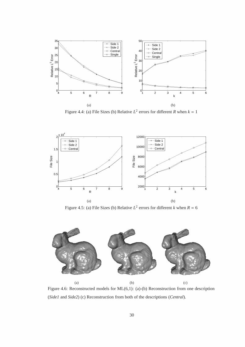
4 5 6 7 8 90

5

10

15

20

25

30

35

R

Rel

ativ

e L2 E

rror

Side 1Side 2CentralSingle

(a)

1 2 3 4 5 60

10

20

30

40

50

k

Rel

ativ

e L2 E

rror

Side 1Side 2CentralSingle

(b)

Figure 4.4: (a) File Sizes (b) RelativeL2 errors for differentRwhenk = 1

4 5 6 7 8 90

0.5

1

1.5

2x 10

4

R

File

Siz

e

Side 1Side 2Central

(a)

1 2 3 4 5 62000

4000

6000

8000

10000

12000

k

File

Siz

e

Side 1Side 2Central

(b)

Figure 4.5: (a) File Sizes (b) RelativeL2 errors for differentk whenR= 6

(a) (b) (c)

Figure 4.6: Reconstructed models for ML(6,1): (a)-(b) Reconstruction from one description

(Side1andSide2) (c) Reconstruction from both of the descriptions (Central).

30

Table 4.3: File Sizes for differentk whenR= 6

Model ML 6,1 ML 6,2 ML 6,3 ML 6.4 ML 6,5 ML 6,6

Side 1 3548 4842 5728 7071 7902 8939Side 2 3546 4840 5564 6980 7782 8958Central 4715 6305 7452 8739 9805 10762

Table 4.4: RelativeL2 errors for the case in Table 4.3

Model ML 6,1 ML 6,2 ML 6,3 ML 6.4 ML 6,5 ML 6,6

Side 1 16,48 26,41 29,18 34,95 37,13 40,30Side 2 17,43 25,57 28,69 34,11 35,43 39,59Central 6,15 4,39 3,54 3,06 2,76 2,47Single 6,84 4,90 4,24 3,34 2,98 2,64

4.3 Proposed Tree Partitioning

This MDC approach [1] is also based on Progressive Geometry Compression (PGC) scheme

while it can be adapted to any mesh coding scheme employing wavelet transform and zero-

tree coding. In order to obtain multiple descriptions, wavelet coefficient trees are grouped

into several sets which are to be independently coded. Thesesets are packetized into multiple

descriptions in such a way that each description contains one tree set which is coded with

higher rate and several redundant tree sets which are coded with lower rates.

The general scheme is shown in (Figure 4.7). Wavelet coefficient trees are split into several

setsWi , i = 1 . . .N and coded by SPIHT algorithm with high bitrate. Each description con-

tainsM copies of different tree sets (M ≤ N). Namely,Description icontains one setWi coded

at rateRi,0 andM−1 sets of redundant treesWj , j , i. TheseM−1 tree sets represent coding

redundancy and are coded at lower rates thanRi,0. The redundancy included in each descrip-

tion is obtained as a result of the optimization algorithm described in following paragraphs.

As the most important information in the embedded stream is located at the beginning of the

bit-stream, the redundant copies would be used if the descriptions with corresponding high-

rate coded tree subsets are lost. If some descriptions are lost, the most important parts of the

original trees in those descriptions will be recovered because their copies at lower rates will

be present in the received descriptions. The compressed coarsest mesh representationC with

rateRC is included in every description to facilitate the inverse wavelet transform even if only

one description is received. Duplicating coarsest meshC also increases coding redundancy.

31

Figure 4.7: TM-MDC encoder scheme.

The way of grouping the coefficient trees into sets is particularly important, since different

sets are reconstructed with different quality in case of description loss. Therefore, 3D mesh

locations corresponding to different tree sets will have different quality. To perform grouping

of trees into sets, ordering of the coarsest mesh vertices isperformed, as proposed in [83, 84].

It provides ordering of the vertices that has good locality and continuity properties. Then,

the desired type of wavelet trees grouping is obtained by sampling the one-dimensional array

[83, 84]. Two types of tree set splitting have been compared:first - grouping the closely

located trees together and second - grouping spatially disperse trees. The spatially close

grouping is obtained by assigning successive vertices fromthe array to the same group. The

disperse grouping is obtained by sampling the array in a round-robin fashion. It has been

observed the latter case yields annoying artifacts in case when only one description is received

and that the former case given better visual quality in general. This is illustrated in Figure 4.8

where modelBunnyis encoded into four descriptions and optimized for PLR= 15%. One

can see that although grouping disperse disperse trees achieves lower objective distortion than

grouping close trees, it produces annoying visual artifacts. Therefore remaining results of this

work are obtained by spatially close grouping method.

Redundancy of the proposed algorithm is determined by the number of redundant tree copies,

their rates and the coarsest mesh size. Bit allocation problem has to minimize expected distor-

tion at the decoder subject to probability of packet lossP and the target bit budget. A simple

channel model where probability of packet lossP for each packet is assumed to be the same

and independent of previous channel events is used. Anotherassumption is that one packet

corresponds to one description. If the description has to befragmented into different packets,

probability of the description lossP can be found from PLR.

Suppose thatN descriptions are generated. Then, coefficient trees are split intoN tree sets,

32

(a) PSNR= 50.73 dB (b) PSNR= 48.51 dB

Figure 4.8: Reconstruction of modelBunnyfrom one description among four descriptionsfor different types of tree grouping. (a) Spatially disperse grouping; PSNR= 50.73 dB. (b)Spatially close grouping, group size is 10; PSNR= 48.51 dB.

and M copies of tree sets are included in one description (M ≤ N). Given P, it is easy to

determine for each copy of the tree set the probabilitiesPi , i = 0, . . .M that this copy is used

for reconstruction whereP0 is the probability of using the full-rate copy of the tree set, and

PM is the probability of not receiving any copy of the tree set. ProbabilitiesPi can easily

be found fromP and the packetization strategy. Thus, we have to minimize the expected

distortion

E[D] =N

∑

i=1

M∑

j=0

P jDi j (Ri j ), (4.1)

whereDi j is the distortion incurred by usingj-th copy of a tree seti andRi j represents bits

spent for j-th copy of i-th tree set. Optimization is performed under following bitrate con-

straintsN

∑

i=1

M∑

j=0

Ri j + NRC ≤ R, (4.2)

whereR is the target bitrate andNRC is the rate of the coarsest mesh. The rate of the coarsest

mesh is chosen constant with geometry information quantized to 14 bitplanes.

Optimization of bit allocation requires computation ofD(R) function for every allocation

step. Calculation ofD(R) is a computationally expensive operation. However, each tree set

contributes to total distortionD. Since each tree set corresponds to some separate location on

the mesh surface (defined by the root edge) in grouping spatially close trees, the distortions

corresponding to separate tree sets can be considered additive. Therefore, distortion-rate (D-

R) curveDi(Ri) for each coefficient tree set is obtained in advance. Calculations ofDi(Ri) are

33

performed only once before the optimization algorithm is used for the first time. Then D-R

curves are saved and can be used every time in bit allocation algorithm for new values ofR

andP.

Optimization is performed with generalized Breiman, Friedman, Olshen, and Stone (BFOS)

algorithm [85]. BFOS algorithm first allocates high rate foreach copy of the tree set. Then,

the algorithm consequently deallocates bits from the sets whereD(R) curves shows the lowest

decay at allocated bitrate. This process stops when bit budget constraints are satisfied. In case

optimization brings zero rates for some redundant trees copies, these copies are not included

in the descriptions.

The embedded bitstream can be stopped literally at any point. Thus, calculation of the whole

D-R curve requires considerable time. Therefore we employ the Weibull modeling of D-R

curve presented in [86] for coding of images. It has been shown in [1] that the output of PGC

coder can also be approximated with this model. The model is described by

D(R) = a− be−cRd, (4.3)

where real numbersa, b, c, andd are the parameters which depend on the D-R character-

istics of the compressed bitstream. As there are four parameters in this model,D(R) curve

can be found by using at minimum four points. This model can approximate bothL2 and

PSNR curves. To fit this model to D-R samples, we use nonlinearleast-squares regression.

Figure 4.9 shows the comparison of true operational D-R curves ofBunnymodel and their

Weibull models. One can see that the model closely approximates the real data. Moreover,

the model has a nice feature of convexity, which is desirablefor bit allocation algorithm.

Experiments are performed for modelsBunnyandVenus head. The original uncompressed

models are shown in Figure 4.3. In the experiments, modelBunny is coded into four de-

scriptions at total 22972 Bytes (5743 Bytes per description) and eight descriptions at total

25944 Bytes (3243 Bytes per description). ModelVenus headis coded into four descriptions

at 24404 Bytes (6101 Bytes per each description). The reconstruction distortion metric is

the same metric as in Section 4.2 which is relativeL2 distance. Also the same numbers are

provided in PSNR scale where PSNR= 20 log10 peak/d, peak, peak is the bounding box

diagonal, and d is theL2 error.

34

0 5 10 15 200

10

20

30

40

50

Size (kbytes)

Rel

ativ

e L2 E

rror

True functionWeibull model

(a)

0 5 10 15 2040

45

50

55

60

65

70

75

Size (kbytes)

PS

NR

(dB

)

True functionWeibull model

(b)

Figure 4.9: Comparison between the Weibull model (10 points) and operational D-R curve(L2) for Bunnymodel. (a) RelativeL2 error; (b) PSNR.

In the experiments, three coders are compared. The first coder is the one proposed in the

algorithm, which is named Tree-based Mesh MDC (TM-MDC). Thesecond coder is a simple

MDC coder in which each description contains the coarsest mesh and one set of wavelet

coefficient trees. The sets of coefficient trees in both coders are formed from spatially close

groups of trees of size 10. This coder is the same as TM-MDC optimized for P = 0 (for

P = 0, no redundant trees are included in the descriptions). Thethird coder is unprotected

SPIHT. The packetization for unprotected SPIHT is performed in the following way. The

output bitstream of PGC coder is divided intoN parts of equal size, whereN is the number

of descriptions in the MD coder that unprotected SPIHT is compared to. PGC produces the

embedded bitstream. Thus, the received part can be used for reconstruction if all the packets

containing earlier parts of bitstream have been received. For example, if parts one, two, and

four are received, only parts one and two are used for reconstruction. If part one is lost, no

reconstruction is available.

Figures 4.10 and 4.11 show the average distortions for reconstruction from different number

of received descriptions for modelBunnycoded into four and eight descriptions respectively.

The curves are generated for TM-MDC with bit allocations optimized for differentP. From

the figures, it is observed that when all of the descriptions are not received, the coder opti-

mized for higherP has the best PSNR value. However this does not mean that higher loss

rates lead to better performance because the coder is optimized to minimize expected distor-

tion driven by the packet loss rate. Therefore since the coder optimized for a high loss rate

expects more description losses, it tries to achieve betterdistortion in cases when small num-

35

ber of descriptions are received. On the other hand, the coder optimized for a low loss rate

is expected to receive more descriptions and it tries to achieve better distortion in cases when

most of the descriptions are received. This can be verified from the figures by the observing

that the coder optimized forP = 1% shows the best performance in case all descriptions are

received.

1 2 3 40

10

20

30

40

50

Number of descriptions received

Dis

tort

ion

PLR 1% (ρ=25%)PLR 3% (ρ=37%)PLR 5% (ρ=47%)PLR 15% (ρ=73%)

(a)

1 2 3 445

50

55

60

65

70

75

80

Number of descriptions receivedP

SN

R (

dB)

PLR 1% (ρ=25%)PLR 3% (ρ=37%)PLR 5% (ρ=47%)PLR 15% (ρ=73%)

(b)

Figure 4.10: Reconstruction ofBunnymodel from different number of received descriptions.The results are given for bit allocations for different packet loss rates (PLR). The redundancyρ is given in brackets. (a) RelativeL2 error; (b) PSNR.

1 2 3 4 5 6 7 80

20

40

60

80


PS

NR

(dB

)

PLR 5% (ρ=68%)PLR 10% (ρ=87%)Unprotected SPIHT

Figure 4.11: ModelBunnyencoded into 8 descriptions at total 25944 Bytes. Reconstructedfrom different number of descriptions. Compared to unprotected SPIHT.

Figure 4.16 compares the performance of the proposed TM-MDC, the simple MD coder, and

unprotected SPIHT for modelBunny. The results are calculated forP = 0, 1, 3, 5, 10, 15, 20%.

36

0 5 10 15 200

5

10

15

20

25

30

35

Packet loss rate (%)

Rel

ativ

e L2 e

rror

TM−MDC (L2 dist.)TM−MDC (Weibull)Simple MDC

(a)

0 5 10 15 2020

30

40

50

60

70

80


PS

NR

(dB

)

TM−MDC (L2 dist.)TM−MDC (Weibull)Simple MDCUnprotected SPIHT

(b)

Figure 4.12: The comparison of network performance of the proposed TM-MDC with a sim-ple MDC scheme and unprotected SPIHT. (a) RelativeL2 error; (b) PSNR.

In TM-MDC coder, bit allocation is optimized for each P. For simple MDC coder, redundancy

is always fixedρ = 10% which occurs due to including coarsest level data in eachdescription.

For eachP, the average distortion is calculated by averaging resultsof 100000 experiments

(simulations of packet losses). ForP = 0, coders show the same performance because the

optimized forP = 0 TM-MDC coder and simple MDC coder are in fact the same coder.

However, for higher packet loss rates, the performance of simple MDC coder dramatically

decreases while the reconstruction quality of TM-MDC showsonly mild degradation. For

P = 20%, the optimized TM-MDC coder is 15 dB higher than the simple MD coder.

In the figure, TM-MDC method results are shown for two different labels, namely TM-MDC

(L2 dist) and TM-MDC (Weibull). The former corresponds to the results obtained by us-

ing original D-R curves in optimization while the latter corresponds to results obtained by

modeling D-R curves by Weibull model [86] to decrease complexity.

Figure 4.13 shows visual reconstruction results for the model Bunnywhich is encoded with

redundancyρ = 63% and Figure 4.14 shows visual reconstruction results forthe modelVenus

headwhich is encoded with redundancyρ = 53%. The reconstructed visual models corre-

spond to reconstructions from one, two, three, and four description. One could see that even

the reconstruction from one description provides acceptable visual quality.

37

(a) (b)

(c) (d)

Figure 4.13: Reconstruction of theBunnymodel from (a) one description (48.36 dB), (b) twodescriptions (63.60 dB), (c) three descriptions (71.44 dB), (d) four descriptions (74.33 dB).

38

(a) (b)

(c) (d)

Figure 4.14: Reconstruction ofVenus headmodel from (a) one description (53.97 dB), (b)two descriptions (65.18 dB), (c) three descriptions (72.51dB), (d) four descriptions (77.08dB).

39

4.4 Proposed FEC Based Approach for MDC

This approach can be used for both MDC [4] and packet loss resilient streaming [5]. The

packet loss resilient streaming analysis is provided in Section 4.5. Our aim is to achieve best

reconstruction quality with respect to channel bandwidth and packet loss rate (PLR). The

proposed algorithm adapts the FEC based packet loss resilient image coding schemes [87].

The algorithm first generates an embedded bitstream by compressing the mesh with PGC

algorithm. The bitstream is protected by optimal FEC assignment.

4.4.1 Problem Definition and Proposed Solution

In this work, we try to minimize the expected reconstructiondistortion of the 3D model trans-

mitted over an erasure channel for a given target bit-rate,PLR and channel model. In order to

achieve this, first the 3D model is compressed with PGC as described in Section 3.1.1 and an

embedded bitstream is produced. After the embedded bitstream is produced, the problem of

optimum loss protection is stated as follows: The embedded bitstream is protected with RS

codes and transmitted over an erasure channel inN packets each with the length ofL symbols

(bytes in this work). The protection system buildsL source segmentsSi , i = 1, ..., L which

have the lengthsmi ∈ {1, ...,N} and protects each segment with anRS(N,mi) code. For each

i = 1, ..., L, let fi = N −mi denote the number of RS redundancy symbols protecting the seg-

mentSi. An example of this FEC assignment is illustrated in Table 4.5. If n out of N packets

are lost, then the RS codes ensure that all the segments that contain at mostN − n source

symbols can be recovered. Adding the constraintf1 ≥ f2 ≥ ... ≥ fL, one can be sure that if

fi packets are lost, then the receiver can decode at least the first i segments. LetF denote the

set ofL-tuples (f1, ..., fL) such thatfi ∈ {0, ...,N− 1} for i = 1, ..., L and f1 ≥ f2 ≥ ... ≥ fL. Let

p(m,N) denote the probability of losing exactlympackets out ofN and let

cN(k) =k

∑

m=0

p(m,N) for k = 0, ...,N (4.4)

Then cN( fi) is the probability that the segmentSi can be decoded successfully. LetD(R)

denote the distortion-rate (D-R) function of the source coder. In order to achieve an optimum

packet loss protection, we need to findF = ( f1, ..., fL) ∈ F such that the expected distortion

40

ED = cN(N)D(r0) +L

∑

i=1

cN( fi)(D(r i) − D(r i−1)) (4.5)

is minimized where

r i =

0, for i = 0

∑ik=1 mk = iN −

∑ik=1 fk, for i = 1, ..., L

(4.6)

Note that the D-R curve modeling introduced in Section 4.3 isalso applicable during the

optimization of this problem.

The next step is to determine the optimum FEC assignments by minimizing ED in Equation

4.5. In the literature, there are several efficient methods for similar optimization problems

used for scalable image coders [87], [88], [89], [90], [91],[92]. In [91], it is shown that the

method in [88] performs very well in terms of expected distortion and the method in [91] has

the lowest computational complexity with slightly worse expected distortion performance.

In [88], given p = LN points on the operational D-R curve of the source coder, the algorithm

first computes theh vertices of their convex hull. Then, the solution is found inO(hN logN)

time. This solution is optimal under the assumption of the convexity of the D-R function

and of fractional bit allocation assignment. In [91], a local search algorithm withO(NL)

complexity is presented that starts from a solution that maximizes the expected number of

received source bits and iteratively improves this solution. The reader is referred to [88], [91]

for the details of the algorithms. Since we also use a scalable bitstream produced by PGC

coder, we employ in our experiments the optimization methods from [88] and [91].

Table 4.5: An example FEC assignment on an embedded bitstream. There areN = 5 packetseach composed ofL = 4 symbols. Therefore there are 4 source segments,Si, i = 1, 2, 3, 4each of which containsmi data symbols andfi FEC symbols wheremi + fi = N. In thisexamplem1 = 2, f1 = 3,m2 = 3, f2 = 2,m3 = 3, f3 = 2,m4 = 4, f4 = 1. Earlier parts of thebitstream are assigned more FEC symbols since they contribute more to overall quality.

P1 P2 P3 P4 P5

Segment 1 1 2 FEC FEC FECSegment 2 3 4 5 FEC FECSegment 3 6 7 8 FEC FECSegment 4 9 10 11 12 FEC

41

4.4.2 MDC Experimental Results

In this part of the experiments, we try to obtain the MDC performance of the proposed method.

We compare the proposed coder with the coder TM-MDC of previous section [1]. We have

performed the experiments on modelBunny. In the experiments, modelBunnyis coded at

22972 Bytes (5743 Bytes per each description). The reconstruction distortion is the relative

L2 error and PSNR values are calculated as in previous sections.

In the experiments, Figure 4.15 shows reconstruction from different number of descriptions.

In the figure, labelL2 distancemethod corresponds to usingL2 distance obtained by metro

tool, approximate L2 distance method corresponds to using approximateL2 distance value

obtained by disabling face and edge samplings in metro tool and labelWeibull modelmethod

corresponds to usingD(R) curve obtained by modeling originalD(R) curve with 10 values of

L2 distances during optimization procedures. Both MDC codersare optimized for PLR= 5%.

As one can see, both MD coders outperform unprotected SPIHT except for the case, when all

the descriptions are received. The TM-MDC achieves higher PSNR for reconstruction from

one description, but lower PSNR for reconstruction from three descriptions. We think that this

can be strongly connected with the fact that each description in TM-MDC method includes

whole coarsest level geometry while descriptions in our method does not contain all bitplanes

of coarsest level geometry. Another observation is that results of L2 distance, approximate

L2 andWeibull modelmethods are indistinguishable in the figure which proves thesuccess of

modeling.

1 2 3 40

20

40

60

80


Rel

ativ

e L2 e

rror

TM−MDC

L2 distance

Approx. L2 dist.Weibull model

(a)

1 2 3 40

20

40

60

80


PS

NR

(dB

)

TM−MDC

L2 distance

Approx. L2 dist.Weibull modelUnprotected SPIHT

(b)

Figure 4.15: Reconstruction from different number of descriptions (PSNR) forBunnymodel.(a) RelativeL2 error; (b) PSNR.

42

0 5 10 15 200

2

4

6

8

10

12


Rel

ativ

e L2 e

rror

TM−MDCWeibull model

(a)

0 5 10 15 2020

30

40

50

60

70

80


PS

NR

(dB

)

TM−MDCWeibull modelUnprotected SPIHT

(b)

Figure 4.16: The comparison of the MD-FEC with TM-MDC coder from [1]. (a) RelativeL2

error; (b) PSNR.

Figure 4.16 compares the average performance in the lossy environment of the proposed coder

usingL2 distance, approximateL2 distance, Weibull model with the performance of unpro-

tected SPIHT and TM-MDC coder from [1]. As seen in the figure, the proposed approach

shows competitive results compared to TM-MDC and considerably outperforms unprotected

SPIHT.

4.5 Extension of MD-FEC to Packet Loss Resilient Coding

In this section, we extend the MD-FEC approach described in the previous section to be used

in packet loss resilient streaming scenarios by simply increasing the number of descriptions

to achieve smaller and meaningful packet sizes for common network protocols. This would

not be possible with the TM-MDC method since increasing the number of descriptions bring

extra redundancy.

We compare our results with the state of the art CPM based methods [78],[80] in terms of

expected distortion and flexibility in packetization. Therefore, we first provide an overview

of CPM based loss resilient coding approaches. In the literature, CPM based methods were

tested only with 3D models with small number of triangles. Inthis work by decreasing the

complexity, we manage to do the performance evaluation for 3D models with high number of

triangles. The experimental results show that, higher quality with more flexible packetization

can be achieved by the proposed algorithm.

43

4.5.1 Packet Loss Resilient Coding Based on CPM

The compression algorithm of CPM was described in Section 3.1.2. For loss resilient trans-

mission of the data generated by the CPM algorithm, optimal error correcting codes (in par-

ticular Reed-Solomon - RS codes) can be assigned to the layers of the progressively coded

mesh. LetRS(N, k0) denote the RS code applied to base layer (level-0) andRS(N, k j) denote

the RS code applied to j-th enhancement layer (level-j), where j = 1, ..., LM. HereLM denotes

the number of enhancement layers transmitted out ofM enhancement layers according to the

bitrate of the channel. RS codes are applied vertically and packetization is performed hori-

zontally. Therefore receiving anyk j out of N packets of level-j allows successful decoding

of level-j. A simple protected CPM output bitstream is illustrated in Table 4.6. A drawback

of this packetization is that since N andR(i) are constant, packet sizes of different layers vary

for different assignments ofk j values, which is not the case in wavelet based loss resilient

techniques. Padding the shorter packets with zeros would cause an increase in the bandwidth

requirements.

Table 4.6: An example CPM output withLM + 1 = 3 layers.Pi denotes Packeti generatedhorizontally while FEC is applied vertically. In this simple exampleN = 6, k0 = 2, k1 = 3andk2 = 4.

Base Mesh Batch 1 Batch 2

P1 1 2 P7 5 6 P13 11 12 13P2 3 4 P8 7 8 P14 14 15 16P3 FEC FEC P9 9 10 P15 17 18 19P4 FEC FEC P10 FEC FEC P16 20 21 22P5 FEC FEC P11 FEC FEC P17 FEC FEC FECP6 FEC FEC P12 FEC FEC P18 FEC FEC FEC

The problem definition can be formulated as follows: Given a 3D model and a total bit budget

B, the aim is to determine an optimal combination of the following parameters to minimize

the expected decoded model distortion (ED(LM)): 1) l, number of bits used in quantizing the

position error; 2)LM, the number of transmitted batches; 3)C, the total number of channel

coding bits; 4)CL = [C(0),C(1), ...,C(LM)], C(i) denoting the number of channel coding bits

applied to leveli (or [k0, k1, ..., kLM ] sinceki is a function ofC(i), R(i) andN).

To quantify the expected distortionED(LM), first let P j denote the probability of terminating

the decoding operation at level-j and it can be calculated as

P j =

N∑

m=N−kj+1

p(m,N) (4.7)

44

where p(m,N) is the probability of losingm packets within a block ofN packets. Then

expected distortionED(LM) can be calculated as

ED(LM) = P0DNR+

LM∑

j=1

P jD j−1

j−1∏

i=0

(1− Pi) + DLM

LM∏

j=0

(1− P j) (4.8)

whereD j is the distortion of level-j,DNR is the distortion when no reconstruction of the model

is possible (i.e. if the base mesh is lost),DLM is the distortion if all the levels are successfully

received.

4.5.2 Proposed Modifications for CPM based Loss Resilient Coding

AlRegib et al. [78] propose an algorithm to find the optimal solution for this problem. Ac-

cording to the distortion-rate (D-R) curves, the algorithmselects the best (l, LM) pair by

varyingC values using a step sizeQ. For each selectedl andLM, the lowest expected distor-

tion andCL are found using a local search algorithm. Final output of thealgorithm is theCL

corresponding to lowest distortion among all steps.

A drawback of this algorithm is that it contains many repeated operations since the results are

iterated by varyingC using the step sizeQ. As there are finite choices ofl, LM andk j values

for aC, it is very likely to encounter samel, LM andk j values for severalC values during the

local search. In [77], this computational redundancy is removed by iterating only the finite

k j values and putting the constraint thatk0 ≤ k1 ≤ ... ≤ kL. Although in [77] the problem

definition also assumes thatC is given andLM is fixed, we can generalize the algorithm by

removing this assumption. In our experimental results, we combine the two methods such

that, for given possible finite sets ofl’s andLM ’s:

• The combined algorithm computes expected distortion for every k j values satisfying

the bit budget requirement and thek0 ≤ k1 ≤ ... ≤ kL condition.

• k j values corresponding to the least expected distortion is chosen as the optimum FEC

assignment.

AlRegib et al. [79] tackle with a similar problem in whichl is also assumed to be given

in addition to our general problem definition. An exhaustivesearch of [C(0),C(1), ...,C(L)] is

45

proposed to find the optimal solution. In [80], Ahmad et al. propose improvements on [79]

in terms of complexity and packetization flexibility inspired from the work in [92]. In our

experimental results, in order to obtain Ahmad et al.’s results, we first find the local optimum

parameters for all possiblel values. Then the parameters corresponding to the lowest expected

distortion is chosen as the global optimum parameters.

4.5.3 Distortion Metric and Simplifications in Calculations

In order to use Equations (4.8) and (4.5), the distortionsD j andD(R) are chosen asL2 distance

as in previous sections. To reduce complexity ofL2 distance computations, modeling D-

R curve with Weibull Model is employed as in Section 4.3. For CPM based methods, this

complexity is decreased by using quadric error metric as proposed in [77].

4.5.4 Channel Model

In order to take into account the packet loss behavior to minimize the expected reconstruction

distortion, the channel is needed to be modeled appropriately. In this work, we use a two-state

Markov model which is shown to be very effective in modeling packet losses [93], [94].

1 - pGB

1 - pBG

PBG

PGB

B G

Figure 4.17: Two state Markov channel model.

The Markov model described in [93] and [94] is a renewal model, i.e., the event of a loss resets

the memory of the loss process. Such models are determined bythe distribution of error free

intervals (gaps). Let a gap of lengthv be the event that after a lost packet,v − 1 packets are

received and then again a packet is lost. The gap density function g(v) gives the probability

of a gap lengthv, i.e.,g(v) = Pr(0v−11|1), where ’1’ denotes a lost packet and ’0v−1’ denotes

v− 1 consecutively received packets. The gap distribution functionG(v) gives the probability

46

of a gap length greater thanv− 1, i.e.,G(v) = Pr(0v−1|1). In our model, in state B all packets

are lost (’1’), while in state G all packets are received (’0’), yielding

g(v) =

1− pBG, if v = 1

pBG(1− pGB)v−2pGB, if v > 1(4.9)

G(v) =

1, if v = 1

pBG(1− pGB)v−2, if v > 1(4.10)

Let R(m,N) be the probability ofm− 1 packet losses within the nextN − 1 packets following

a lost packet. It can be calculated using the recurrence.

R(m,N) =

G(N), m= 1

∑N−m+1v=1 g(v)R(m− 1,N − v), 2 ≤ m≤ N

(4.11)

Then the probability ofm lost packets within a block ofN packets given in Equations 4.4 and

4.7 is

p(m,N) =N−m+1∑

v=1

PBG(v)R(m,N − v+ 1), if 1 ≤ m≤ N (4.12)

wherePB is the average loss probability.

4.5.5 Experimental Results

In this part of the experiments, we try to obtain the packet loss resilient streaming performance

of the proposed method where the number of packets are much higher compared to MDC

case. We compare the proposed method with CPM based methods.We have used the test

modelsBunnyand Venus head. The packets are sent over the two-state Markov modeled

packet erasure channel with the average burst length of 5. All the experiments are performed

using an Intel Pentium 4 2.2GHz 1Gb RAM Windows XP installed computer. Although it is

not possible to estimate exact complexity with these settings (e.g. due to possible inefficient

implemented parts of algorithms or multitasking of OS), we provide the results to mention

the order of complexity of the algorithms compared to each other.

47

In the following experimental results, if the 3D model name and the coding bitrate are not

explicitly specified, then these results correspond to theBunnymodel coded at 3.5 bpv and

packetized withN = 100.

In the rest of this section, we categorize the experiments and present in different subsections.

We start with the results of CPM based methods which include the proposedkS tepparameter

and comparison of CPM based method simulation distortions.Then we provide the results for

D-R curve modeling for PGC based methods followed by the comparison of CPM and PGC

based methods in terms of simulation distortions. Then we examine the mismatch scenario

which occurs when the real loss rate and the one used in optimization differ. We continue

the results with complexity comparisons for the optimization methods and finally we provide

visual results for subjective evaluation.

4.5.5.1 Proposed kStep for CPM Based Methods

For AlRegib’s CPM based methods, since iterating all possible RS(N, k j) pairs for each layer

is not feasible due to significant complexity requirements,we propose a new parameterkS tep.

With kS tepparameter, instead of iteratingk j ’s in RS(N, k j) pairs one by one, we increment

and decrementk j values by an amount ofkS tepin the iterations. Figure 4.18 shows the

simulated PSNR values and Figure 4.19 shows the optimization times for differentkS tep

values.

2 3 4 5 6 7 8 9 1059.5

60

60.5

61

61.5

62

62.5

k Step Size

PS

NR

(dB

)

AlRegib PLR=2%AlRegib PLR=4%AlRegib PLR=10%

Figure 4.18: Effect of k step size on quality: Simulated PSNR vs k step size forBunnymodeloptimized forPLR = 2%, 4% and 10% and coded at 3.5 bpv.

48

3 4 5 6 7 8 9 100.01

0.1

1

10

100

1000

k Step Size

Opt

imiz

atio

n T

ime

(sec

)

Figure 4.19: Effect of k step size on complexity: Optimization time vs k step size for Bunnymodel optimized forPLR = 4% and coded at 3.5 bpv.

From the figures, it can observed that it is possible to save great amount of time during op-

timization by increasing thekS tepvalue. In addition, while increasing thekS tepvalue, the

decrease in the simulated PSNR value is not significant for different packet loss rates.

4.5.5.2 Comparison of CPM Based Methods

0 10 20 30 4055

57

59

61

63

65


PS

NR

(dB

)

AlRegib kStep = 2AlRegib kStep = 5AlRegib kStep = 5 QuadAhmadAhmad Quad

Figure 4.20: Comparison of CPM based methods for Bunny modelin terms of simulateddistortions for variousPLR’s.

After defining thekS tepparameter, we proceed to comparison of all aforementioned CPM

based methods. Figure 4.20 summarizes all of the mentioned CPM based error resilient meth-

49

ods. In the figure, simulated PSNR vsPLR values are presented for several configurations.

The curves in the figure are AlRegib’s method with a finekS tepvalue of 2 (AlRegib kStep=

2), AlRegib’s method with a coarserkS tepvalue of 5 (AlRegib kStep= 5), AlRegib’s method

with kS tep= 5 and using quadric error metric during optimization (AlRegib kStep= 5 Quad),

generalized Ahmad’s method (Ahmad) and generalized Ahmad’s method with using quadric

error metric during optimization (Ahmad Quad).

From the figure, it can be deduced that all the CPM based methods similar performance,

where none of the methods achieve significantly higher simulated PSNR. Nonetheless, best

PSNR is achieved byAlRegib kStep= 2 as expected.

4.5.5.3 Performance of D-R Curve Modeling for PGC Based Methods

After examining the CPM based methods, we start the analysisof PGC based methods. For

the PGC based methods, FEC assignments are optimized with the algorithms of Mohr et al.

[88] and Stankovic et al. [91] and labeled asPGCMohrandPGCStankovicin the rest of the

chapter.

We initially examine the performance of the proposed D-R curve modeling described in pre-

vious sections. Figure 4.21 shows simulated distortions corresponding to variousPLR’s for

PGCMohremploying the original D-R curve and modeled D-R curve during optimization. It

is observed that quite acceptable results can be achieved byD-R curve modeling. Therefore

we present the remaining PGC based results with modeled D-R curves which significantly

reduce optimization times.

4.5.5.4 Comparison of CPM and PGC Based Methods

In this part, we present comparison of the CPM and PGC based methods in terms of simulation

distortions for three cases: 1) Bunny Model Coded at 3.5 bpv,2) Bunny Model Coded at 1.2

bpv and 3) Venus Model Coded at 4 bpv.

Bunny Model Coded at 3.5 bpv

For this case, a comprehensive summary of the results for allmethods is presented in Table

4.7. Also comparison of CPM based and PGC based methods in terms of simulated PSNR can

50

0 10 20 30 4062

64

66

68

70

72

74

76


PS

NR

(dB

)

Original D−R curveModeled D−R curve

Figure 4.21: Comparison of using original D-R curve and using modeled D-R curve duringoptimization forBunnymodel in terms of simulated distortions for variousPLR’s.

be seen in Figure 4.22. From the results, one can notice that PGC based method significantly

outperform the CPM based methods.

Table 4.7: Simulated distortion results of the first scenario for variousPLR values. The distor-tion metric is relativeL2 error in units of 10−4.

Simulated distortion for differentPLR

PLR values 0% 2% 4% 6% 10% 15% 20% 30% 40%

PGCStankovic 1.89 2.52 2.61 2.78 3.09 3.48 3.78 4.7 5.89PGCmohr 1.85 2.42 2.62 2.66 3.06 3.32 3.87 4.55 6.67

AlRegib kStep=2 6 7.90 8.53 8.78 9.91 11.06 12.30 14.21 17.16AlRegib kStep=5 6 7.94 8.55 8.83 10.00 11.08 12.36 14.32 17.29

AlRegib kStep=5 Quad 6 7.94 8.55 8.83 10.17 11.08 12.36 14.32 17.29Ahmad 6 7.92 8.54 8.82 10.01 11.11 12.35 14.30 17.28

Ahmad Quad 6 7.98 8.55 8.83 10.04 11.16 12.40 14.35 17.28

Bunny Model Coded at 1.2 bpv

In this case, we decrease the bitrate and code Bunny model at 1.2 bpv to observe low bitrate

error resilient characteristics. Comparison of PGC and CPMbased methods is provided in

Figure 4.23. We observe that the results do not change by decreasing the coding bitrate.

Venus Model Coded at 4 bpv

Finally in this case, we repeat the experiments performed onBunnymodel withVenus head

51

0 10 20 30 4055

60

65

70

75


PS

NR

(dB

)

AlRegib kStep = 5PGCStankovicPGCMohr

Figure 4.22:PLR vs Simulated distortion in PSNR scale forBunnymodel coded at 3.5 bpv.

0 10 20 30 4045

50

55

60

65

70


PS

NR

(dB

)


Figure 4.23:PLR vs Simulated distortion in PSNR scale forBunnymodel coded at 1.2 bpv.

52

model which is coded at 4 bpv and packetized withN = 100. Simulated PSNR comparison

of PGC based and CPM based methods can be seen in Figure 4.24. Similar to the results

with the Bunnymodel, we observe that PGC based methods again significantlyoutperform

the CPM based methods.

0 10 20 30 4060

65

70

75

80

85


PS

NR

(dB

)


Figure 4.24:PLR vs Simulated distortion in PSNR scale forVenus headmodel coded at 4 bpv.

4.5.5.5 Mismatch Scenario

In the experiments presented so far, the assumption is that during the optimization we know

the channel loss rate and optimize the protection parameters accordingly. However, in real

cases, the channel packet loss rate used during the optimization and the actual loss rate en-

countered may differ. Therefore in this part, we investigate what happens whena model

optimized for a loss rate is transmitted over a channel with adifferent lost rate. The results of

this experiment are shown in Figure 4.25.

The first observation in the figure is that when the transmission packetization is optimized

for a low loss rate and a channel with a higher loss rate is encountered, the performance

degradation can be severe. On the other hand, when the model encounters a channel with

a lower loss rate, the performance loss is not significant. Another observation is that both

CPM and PGC based methods behave similarly in mismatch scenario and the performance

gap between the methods does not vary.

53

0 5 10 15 20 25 30 35 4025

30

35

40

45

50

55

60

65

70

75


PS

NR

(dB

)

PGC Opt for PLR=2%PGC Opt for PLR=15%PGC Opt for PLR=25%AlRegib Opt for PLR=2%AlRegib Opt for PLR=15%AlRegib Opt for PLR=25%

Figure 4.25:Bunnymodel is coded at 3.5 bpv and FEC assignment is optimized with respectto three differentPLR’s for PGCStankovicandAlRegib kStep= 5 methods. Performance of thethree different assignments for variousPLR’s in terms of simulated distortion in PSNR scale.

4.5.5.6 Complexity Comparison

In the packet loss resilient 3D mesh transmission frameworks presented in this chapter, it

should be noted that the methods are not suitable for real time transmission. The reason is

that the algorithms need to compress the model first and obtain D-R curves, which require

significant amount of time. However, if we are allowed to compress models and store D-R

curves offline, then real time transmission may be possible unless the time spent during the

optimization, so called optimization time, is high. In thiscase, the optimization time of an

algorithm becomes an important measure for real time transmission.

In order to compare the complexities of the optimization parts of the methods, we measured

the optimization time for each algorithm as described at thebeginning of Section 4.5.5. Ta-

ble 4.8 summarizes time requirements for different optimization schemes mentioned in this

chapter.

Table 4.8 shows thatPGCStankovichas the smallest complexity. However, as seen in previous

results, the complexity is smaller than that ofPGCMohr at the cost of occasional slightly

worse simulated PSNR. Examining the CPM based methods, we see thatAhmadandAlRegib

kStep=5 show significantly higher complexity. However, fromkS tep= 8, the complexity

values are comparable with those of PGC based methods.

54

Table 4.8: Optimization times of different methods. Each method is optimized forPLR = 4%

Optimization Times

Methods Time (sec) PSNRPGCMohr 0.250 71.63

PGCStankovic 0.004 71.68Ahmad 11.110 61.37

AlRegib kStep=5 8.350 61.36AlRegib kStep=8 0.365 61.35

4.5.5.7 Visual Comparison of CPM and PGC Based Methods

Apart from the objective distortion metric results, we alsopresent results ofBunny model

coded at 3.5 bpvandVenus head model coded at 4 bpvin terms of visual reconstructions.

Figures 4.26 and 4.27 show visual reconstructions forBunnyandVenus headmodel for vari-

ousPLR values, respectively.

4.6 Conclusions

In this chapter, we have presented various MDC and packet loss resilient coding techniques

for static 3D meshes. In the literature, there was only one work related to MDC of 3D static

meshes [76]. We have proposed three MDC methods, namelyMultiple Description Scalar

Quantization Based Approach[2], Partitioning Wavelet Coefficient Trees Based Approach

[1] andForward Error Correction Based Approach[5] [4]. To compare the techniques, all of

them except the one in [76] are based on wavelet coding. Hencebetter compression ratios and

bitrates for descriptions are obtained in our wavelet basedschemes. Also neither the work in

[76] nor MDSQbased scheme in Section 4.2 does not employ any optimizationwith respect

to varying bandwidth and loss rate of the channel while theTM-MDC method in Section

4.3 andFEC based method in Section 4.4 make use of optimization to significantly improve

expected distortion performance. Moreover, number of descriptions and description sizes can

be adjusted more flexibly inTM-MDC andFEC based methods.

To compareTM-MDC andFEC based methods, although the methods show similar perfor-

mance in terms of expected distortion,FEC based method has several advantages. While

theFEC based method generates one compressed bitstream to optimize FEC assignment for

55

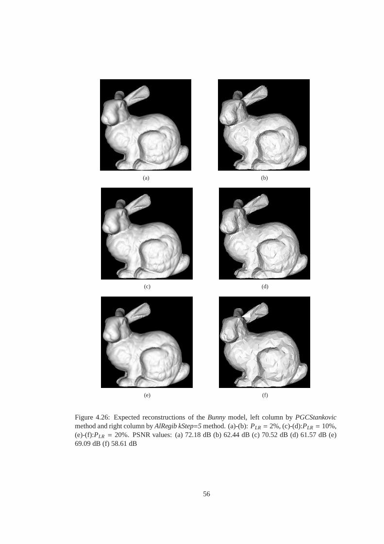
(a) (b)

(c) (d)

(e) (f)

Figure 4.26: Expected reconstructions of theBunnymodel, left column byPGCStankovicmethod and right column byAlRegib kStep=5 method. (a)-(b):PLR = 2%, (c)-(d):PLR = 10%,(e)-(f):PLR = 20%. PSNR values: (a) 72.18 dB (b) 62.44 dB (c) 70.52 dB (d) 61.57 dB (e)69.09 dB (f) 58.61 dB

56

(a) (b)

(c) (d)

(e) (f)

Figure 4.27: Expected reconstructions of theVenus headmodel, left column byPGC-Stankovicmethod and right column byAlRegib kStep=5 method. (a)-(b):PLR = 2%, (c)-(d):PLR = 10%, (e)-(f):PLR = 20%. PSNR values: (a) 76.95 dB (b) 67.79 dB (c) 75.04 dB (d)65.19 dB (e) 74.24 dB (f) 65.19 dB

57

different total number of descriptions,TM-MDC needs to generate different compressed bit-

stream to optimize for different total number of descriptions. The reason is that the set of

wavelet coefficient trees to be assigned to descriptions differs with respect to different total

number of descriptions. ThereforeFEC based method can produce any number descriptions

using the same compressed bitstream whereasTM-MDCmethod needs to have the knowledge

of total number of descriptions to be able to generate bitstreams for optimization of bit allo-

cation for each description. Another advantage ofFEC based method is thatTM-MDC needs

to include whole coarsest level geometry in each description whereasFEC based method

spreads the bitplanes of coarsest level geometry accordingto their importances in compressed

bitstream. In this way more important compressed wavelet coefficients are assigned more

FECs than lower bitplanes of coarsest level geometry and these bitplanes are not included in

each description unless they are assigned repetition codesby optimization algorithm.

As mentioned before, our proposedFEC based method is also used for packet loss resilient

streaming purposes. Regarding to this part, we have presented an extensive analysis of loss

resilient coding methods for 3D models. The methods are based on optimally protecting

compressed bitstreams with FEC codes with respect to given channel bandwidth and packet

loss rate constraints.

We first examined the CPM based methods reported in the literature and came up with a gen-

eral problem definition and solution. We introduced akS tepparameter to iterate protection

rates with different steps and showed that increasingkS tepconsiderably decreases optimiza-

tion times at the expense of very small PSNR degradation.

Then we compared CPM and PGC based methods and experimental results show that PGC

methods achieve approximately 10db better PSNR for all lossrates. It was already reported

in [19] that, compression performance of PGC method is 10dB better than CPM method. In

our results, we show that the 10dB compression performance gap between the methods is

preserved in packet loss resilient transmission. For the same reason, expected reconstructed

models of PGC method at the decoder have a better subjective quality than the ones of CPM

method. We also note that the performance difference may depend on the coarseness of the

model. Apart from the PSNR performance, PGC based methods have an advantage of flexible

packetization. Since the bitstream of PGC method is embedded, the bitstream is generated

only once. Given the channel and bandwidth conditions, the bitstream can be truncated to

58

desired bitrate precisely and FEC assignment is performed easily. The CPM based methods

need to generate different bitstreams for different quantization values and number of bitrate

values that can be achieved is limited.

Finally we simulated performance of optimization methods in a mismatch scenario i.e. the

model is protected with FEC codes optimized for a given loss rate but transmitted through a

channel with a different loss rate. We observed that when the model is optimizedfor a low

loss rate and encounters a channel with a higher loss rate, the performance degradation can

be severe. On the other hand, when the model encounters a channel with a lower loss rate,

the loss in the performance is not significant. Therefore we conclude that when the channel

conditions are uncertain or time varying, it is more robust to optimize loss protection with

respect to a higher loss rate.

59

CHAPTER 5

MULTIPLE DESCRIPTION CODING OF ANIMATED

MESHES

5.1 Introduction

As presented in Section 3.2, recently many works have been proposed for compression of

animated meshes in the literature. On the other hand, there is not much research on trans-

mission and error resilient coding of 3D dynamic meshes. There is only one previous work

[95], where the mesh is spatially partitioned into segmentsand each segment is encoded and

protected by Forward Error Protection (FEC). The disadvantage of the method is that the loss

of some parts of the bitstream means complete loss of corresponding spatial areas. In this

chapter, we focus on MDC of animated meshes as the error resilient tool. Although there are

many works related to MDC of video [13, 15, 96, 14, 97, 98] and MDC of static 3D meshes

[76, 2, 1, 4, 99], MDC of animated mesh data is at a very early stage.

In this work, we propose three MDC schemes for animated 3D meshes. The main differ-

ence between the MDC of static and animated meshes is that theextra dimension of time in

animated meshes brings additional challenges. The first proposed scheme is based on par-

titioning vertices spatially to be encoded independently.This scheme resembles the static

mesh methods in [76] and [1] (TM-MDC) in the sense that spatial partitioning of the vertices

is common in all the methods. However, the proposed method has the additional challenge of

handling reduced compression performance due to inferior temporal prediction. The second

proposed scheme is based on subsampling frames temporally by exploiting the hierarchical B

frame structure, which makes it a completely a different approach compared to static meshes.

The final proposed scheme makes use of the layered scalable structure and is based on du-

60

plicating layers in the descriptions. From the bitstream protection point of view, this scheme

shows similarity to the static mesh approach in [4] (MD-FEC)with two descriptions.

The rest of the chapter is organized as follows. In Section 5.2, we mention the reference dy-

namic mesh coder on which the proposed MDC methods depend. InSection 5.3, we describe

the proposed MDC methods. In Section 5.4, we present the experimental results and finally

we conclude in Section 5.5.

5.2 Reference Dynamic Mesh Coder

The single description (SD) dynamic mesh coder on which our MDC methods is based is

the scalable predictive dynamic mesh coder presented in [66]. The coder can also be viewed

as the layered prediction structure of MPEG-4 FAMC [65] omitting any other modules like

skinning-based motion compensation (SMC). We have chosen this coder as our reference

coder because of both efficient compression performance and the layered structure which

gives flexibility to the design of MD structures. Additionaltools like SMC that improve the

SD compression performance may also be incorporated but this may not necessarily affect

the RRD performance for MDC, i.e. if a tool improving the SD compression improves the

compression of multiple descriptions at the same level, then there is not much RRD perfor-

mance difference. Since the primary focus of this work is to investigate and compare MDC

performances of the proposed methods, we address the possible effects of adding tools that

improve the SD compression performance on the MDC performance as a future work. The

details of the coder, which is referred asReference Dynamic Mesh Coder(RDMC) in the rest

of the text, are provided in Section 3.2.1.

5.3 Proposed MDC Methods

In this section, we describe the proposed MDC methods for dynamic 3D meshes. We propose

three methods which are named after the strategies they are based on:

Vertex partitioning: Based on spatially partitioning the set of vertices into twosets for each

frame.

Temporal subsampling: Based on encoding odd and even frames separately.

61

Layer duplication: Based on duplicating the bitstream corresponding to a subset of layers

and splitting the remaining bitstream for each description.

A common property in all of the methods is that the compressedmesh connectivity is included

in all descriptions. Since we deal with time consistent dynamic meshes whose connectivity

does not change with time, including this data in each description causes very small and

negligible overhead.

5.3.1 Vertex Partitioning Based MDC

5.3.1.1 MD Encoder

In this approach, the first step is to partition the set of all vertices into two disjoint sets where

each set will correspond to a description. The partitioningstrategy affects the MD perfor-

mance since the missing vertices should be concealed from the received ones when only one

of the descriptions is received. For example, an option is cutting the model into halves. In this

case, the received vertices (the ones in the received half) would be compressed and decoded

very efficiently. On the other hand, it would be very difficult to conceal missing vertices (the

ones in the unavailable half) since most of the neighbor vertices would be missing. For this

reason, we try to partition the vertices in both descriptions as dispersed as possible, which

increases the chance of predicting the location of a missingvertex more accurately.

The problem of optimal vertex partitioning to achieve best MDC performance is a difficult

problem. The exhaustive solution is unpractical as it requires too many combinations. There-

fore we focus on a good enough solution which tries to achievedispersed set of vertices rather

than the optimal one. In the literature, the authors in [83, 84] propose an algorithm which pro-

vides 1D ordering of vertices, which has good locality and continuity properties. As a result,

sampling the 1D array with odd and even samples generates twospatially dispersed sets of

vertices. We tested the performance of this partitioning strategy and achieved quite acceptable

MDC performance. Therefore, we adopt this strategy for the vertex partitioning part of the

proposed MDC scheme. We also note that trying other heuristic ad-hoc partitioning methods

resulted in slightly worse performance.

Note that the spatial layered decomposition in the RDMC and the vertex partitioning pre-

62

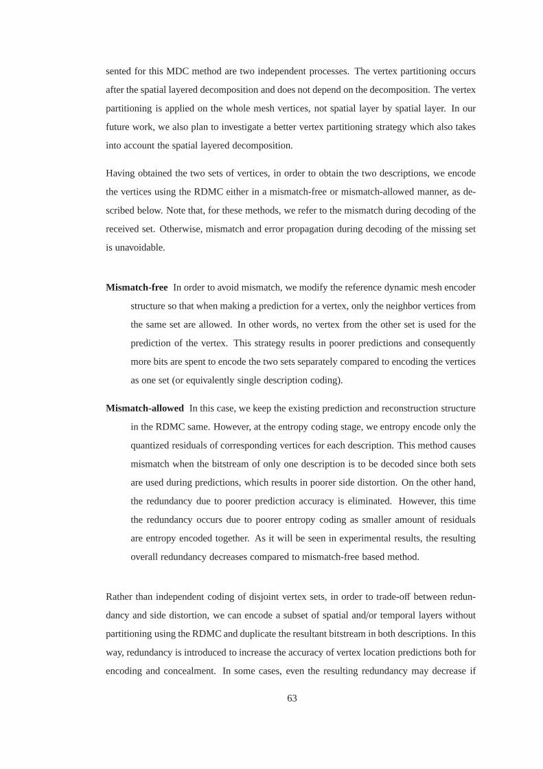
sented for this MDC method are two independent processes. The vertex partitioning occurs

after the spatial layered decomposition and does not dependon the decomposition. The vertex

partitioning is applied on the whole mesh vertices, not spatial layer by spatial layer. In our

future work, we also plan to investigate a better vertex partitioning strategy which also takes

into account the spatial layered decomposition.

Having obtained the two sets of vertices, in order to obtain the two descriptions, we encode

the vertices using the RDMC either in a mismatch-free or mismatch-allowed manner, as de-

scribed below. Note that, for these methods, we refer to the mismatch during decoding of the

received set. Otherwise, mismatch and error propagation during decoding of the missing set

is unavoidable.

Mismatch-free In order to avoid mismatch, we modify the reference dynamic mesh encoder

structure so that when making a prediction for a vertex, onlythe neighbor vertices from

the same set are allowed. In other words, no vertex from the other set is used for the

prediction of the vertex. This strategy results in poorer predictions and consequently

more bits are spent to encode the two sets separately compared to encoding the vertices

as one set (or equivalently single description coding).

Mismatch-allowed In this case, we keep the existing prediction and reconstruction structure

in the RDMC same. However, at the entropy coding stage, we entropy encode only the

quantized residuals of corresponding vertices for each description. This method causes

mismatch when the bitstream of only one description is to be decoded since both sets

are used during predictions, which results in poorer side distortion. On the other hand,

the redundancy due to poorer prediction accuracy is eliminated. However, this time

the redundancy occurs due to poorer entropy coding as smaller amount of residuals

are entropy encoded together. As it will be seen in experimental results, the resulting

overall redundancy decreases compared to mismatch-free based method.

Rather than independent coding of disjoint vertex sets, in order to trade-off between redun-

dancy and side distortion, we can encode a subset of spatial and/or temporal layers without

partitioning using the RDMC and duplicate the resultant bitstream in both descriptions. In this

way, redundancy is introduced to increase the accuracy of vertex location predictions both for

encoding and concealment. In some cases, even the resultingredundancy may decrease if

63

the bitrate saved by better compression due to higher accuracy predictions exceeds the extra

bitrate spent for duplicating the layers. For example, we always duplicated the encoded spa-

tial base layer in both descriptions because the experimental tests showed unacceptably poor

results when the spatial base layer was partitioned into twosets too.The points on the RRD

curves of this algorithm presented in Section 5.4 correspond to various number of spatial and

temporal layers duplicated and the resulting average side distortions.

5.3.1.2 MD Side Decoder

When only one of the descriptions is received, the availableinformation is compressed pre-

diction residuals of the corresponding vertex set and the duplicated spatial/temporal layers.

The general idea in side decoding is to decode received vertices and estimate/conceal the lost

vertices by making use of available vertices.

As the concealment algorithm, we make use of the prediction structures which are already

available from the reference dynamic mesh decoder as it is used to minimize the prediction

error for compression purpose. In the decoding process of anarbitrary frame, vertices in the

frame are decoded in the order of spatial base layer to finest level spatial layer. After the

spatial base layer is decoded, the vertices in the followingspatial layers are predicted using

the vertices from already decoded spatial layers and prediction errors are corrected by using

the information from compressed bitstream. However, in theMD side decoder, only a subset

of the prediction errors are available since the rest of themare lost with the lost description.

Therefore, we assume that prediction errors were encoded aszero and estimate the locations of

missing vertices as the predicted locations in the decoder.Note that during the concealment,

it is not required to use the same prediction method used in the encoder since mismatch is

unavoidable. Therefore either RIC or No-RIC based prediction can be employed.

We can summarize the side decoding process of mismatch-freeMDC for each frame in four

steps:

1. Use the RDMC decoder for the duplicated spatial/temporal layers.

2. Use the RDMC decoder for the vertices from the received description. Note that only

the restricted neighbors from the same description are usedduring spatial prediction.

64

3. Set prediction error residuals of unavailable vertices to zero.

4. Use the RDMC decoder for the unavailable vertices. Note that in this case, there is no

restriction on the neighbors used during spatial prediction since it is already impossible

to match the prediction in the encoder due to losses. We observed that using all the

neighbors during prediction performs the best in the experiments. Also either RIC or

No-RIC based prediction can be employed.

Similarly, we can summarize the side decoding process of mismatch-allowed MDC for each

frame in four steps:

1. Use the RDMC decoder for the duplicated spatial/temporal layers.

2. Entropy decode the received description and obtain dequantized prediction error resid-

uals.

3. Set prediction error residuals of unavailable vertices to zero.

4. For all the vertices, run the RDMC decoder procedures thatfollow the entropy decod-

ing.for all vertices. Either RIC or No-RIC based predictioncan be employed for the

unavailable vertices while for the received vertices, samepredictions as in the encoder

are used.

5.3.1.3 MD Central Decoder

The central decoding is performed when both descriptions are available. In the mismatch-free

version, first the bitstreams of the descriptions are decoded separately and then the separately

reconstructed vertices are combined. In the mismatch-allowed version, first the bitstreams

are entropy decoded separately and prediction error residuals are obtained after dequantizing.

Then the prediction error residuals from the two descriptions are combined and the vertices

are reconstructed using the reference dynamic mesh decoder.

65

5.3.2 Temporal Subsampling Based MDC

5.3.2.1 MD Encoder

In this approach, the mesh frames are split into two sets where each set corresponds to a

description: The first set contains even indexed frames (Frames 0, 2, 4 ... assuming that the

indexing starts from 0) and the second set contains the odd indexed frames (Frames 1, 3, 5

...). In this way, we obtain two new dynamic mesh sequences with a frame rate of half of the

original sequence. Then each sequence is compressed using the RDMC and each description

contains one of the compressed bitstreams. The total bitrate of the descriptions exceed the

bitrate of single description coding because in the MD case,since the frames cannot predict

from the frames in the other set, the interframe prediction efficiency decreases.

F0 F4 F8

SL0,0

SL0,1

SL0,2

SL4,0

SL4,1

SL4,2

SL8,0

SL8,1

SL8,2

SL2,0

SL2,1

SL2,2

SL6,0

SL6,1

SL6,2

SL1,0 SL3,0 SL5,0 SL7,0

F2 F6 F1 F3 F5 F7

F0 F1 F2 F4F3 F5 F6 F7 F8

I0 B3 B2 B4 P1 B7 B6 B8 P5

F1 F2 F4F3 F5 F6 F7 F8

I0 B3 B2 B4 P1 B7 B6 B8 P5

F9

F1 F5 F9 F3 F5 F2 F4 F6 F8

SL1,0

SL1,1

SL1,2

SL5,0

SL5,1

SL5,2

SL9,0

SL9,1

SL9,2

SL3,0

SL3,1

SL3,2

SL5,0

SL5,1

SL5,2

SL2,0 SL4,0 SL6,0 SL8,0

TL1

Description 1

Description 2

TL0 TL2 TL1TL0 TL2

Extra redundancy: one spatial layer from other description

Extra redundancy: one spatial layer from other description

TLi : Temporal Layer i

Figure 5.1: Temporal subsampling based MDC. The example sequence is decomposed intothree temporal layers and three spatial layers. One spatiallayer from the other description isduplicated.

The MD encoding strategy described above results in the minimum possible redundancy and

maximum side distortion for this method. It is also possibleto add more redundancy (increase

in side bitrate) to decrease side distortions. This can be achieved by adding a subset of com-

pressed spatial layers from the other set of frames. The extra number of bits for this procedure

66

is not very high because actually, the frames of the other setare the frames to be encoded in

the last temporal layer in single description case (TL2 in Figure 3.3).

One can notice the relation between the temporal subsampling based MDC and the temporal

layered decomposition in the RDMC. To explain the relation with an example, assume that

our sequence consists of 10 frames (F0, F1, ..., F8 for description 1 andF1, F2, ..., F9 for de-

scription 2) decomposed into three temporal layers and eachframe is decomposed into three

spatial layers as illustrated in Figure 5.1. LetTLi denote the ith temporal layer. For the first

description, initially,F0, F4 andF8 in TL0 are encoded and thenF2 andF6 in TL1 are en-

coded. At this point, one can notice that, we have encoded framesF0, F2, F4, F6 andF8 or

in other words, we have encoded even indexed frames without predicting from odd indexed

frames. This situation corresponds to the lowest possible redundancy case. If we wish to add

more redundancy, we can continue encoding spatial layers from the remainingTL2 which

consists of framesF1, F3, F5 andF7. The amount of redundancy is adjusted by the number

of encoded spatial layers inTL2 frames. For example, if we encode all of the spatial layers

in TL2 frames, then we have a redundancy of 100 % which is equivalentto repetition of the

descriptions. In the example case illustrated in Figure 5.1, one spatial layer from the last tem-

poral layer is included in both descriptions. The points on the RRD curves of this algorithm

presented in Section 5.4 correspond to how many spatial layers of the last temporal layer are

included in each description and the resulting average sidedistortion.

For the second description which corresponds to the odd indexed frames, the same procedures

are applied with the exception thatF1 is considered as the starting frame of the original

sequence as depicted in Figure 5.1.F0 and F9 (first and the last frames) are exceptional

frames for description 1 and 2 respectively and can either beneglected or included in the

encoding process by allowing to predict from the nearest frame.


When only one of the descriptions is received, the received bitstream is fed into the RDMC

decoder. First, all the temporal layers except the last one (which contains frames of the other

set) are decoded in the usual way. Then, if any spatial layersof the last temporal layer (the

extra spatial layers from the frames of the other description) exist in the received description,

the vertices in these spatial layers are decoded in the usualway as well. Finally, for the missing

67

spatial layers, the decoder assumes that the prediction errors for the vertices in these spatial

layers were found to be zero during encoding process. Therefore, the decoder predicts the

vertex locations for the missing spatial layers using either RIC or No-RIC and the predicted

locations are used as the concealed reconstructed locations.

Another possibility is using linear interpolation rather than using the prediction structure in

the decoder. In this approach, the missing vertex locationsare estimated as the average of

corresponding vertex locations from the previous and next frames. In the experimental results,

we compare the performances of using linear interpolation and the prediction structures of the

decoder.


When both of the descriptions are available, each description is fed into the reference dynamic

mesh decoder separately. During the decoding, the decodingof the last temporal layer is

discarded. In this way, decoding one of the descriptions generate only even indexed frames

and the other generates the odd indexed frames. Finally, theeven and odd indexed frames are

combined to generate the mesh sequence at full frame rate.

5.3.3 Layer Duplication Based MDC

5.3.3.1 MD Encoder

The idea of the method is as follows: Initially, the input mesh sequence is compressed with

the RDMC such that the output bitstream consists of two meaningful sub-bitstreams appended

head to tail. The first sub-bitstream is self decodable and decoding results in a lower quality

reconstruction which corresponds to a lower spatial or temporal resolution. The second sub-

bitstream is not self decodable but when it is decoded together with the first sub-bitstream, it

improves the quality of the first sub-bitstream decoding. Therefore the second sub-bitstream

depends on the first sub-bitstream to be decoded. After the sub-bitstreams are generated, the

first sub-bitstream is duplicated in both of the descriptions and the second sub-bitstream is

cut into half so that each half bitstream is placed into a distinct description as illustrated in

Figure 5.2.

68

SL0,0

SL0,1

SL0,2

SL4,0

SL4,1

SL4,2

SL2,0

SL2,1

SL2,2

SL1,0

SL1,1

SL1,2

SL3,0

SL3,1

SL3,2

SL0,0

SL4,0

SL2,0

SL1,0

SL3,0

SL0,1

SL4,1

SL2,1

SL1,1

SL3,1

SL0,2

SL4,2

SL1,2

SL3,2

SL2,2

SL0,0

SL0,1

SL0,2

SL4,0

SL4,1

SL4,2

SL2,0

SL1,0

SL3,0

SL2,1

SL1,1

SL3,1

SL1,2

SL3,2

SL2,2

Border

Self decodable bitstream (duplicated)

Enhancing bitstream (each half to one description)

Transmission order

TL1TL0 TL2

Description 1

Description 2

Half 2Bit

Rate:Re

Half 1Bit

Rate:Re

SelfBit

Rate:Rs

Half 1

Half 2

Self

Self

Example 1 Example 2 Example 3

Figure 5.2: Layer duplication based MDC: three layer ordering examples

The amount of redundancy in this method is equal to the size offirst sub-bitstream as it is

duplicated in both descriptions. Therefore, by playing with the size of first sub-bitstream, the

trade-off between redundancy and side distortion can be adjusted. Dueto the layered structure

(both temporal and spatial) of the RDMC, there are many possible ways to generate the first

sub-bitstream. Figure 5.2 shows three examples for a sequence with 5 frames decomposed

into 3 temporal and spatial layers. In general, assume that the RDMC performsT tempo-

ral andS spatial layer decompositions during encoding. The ordinary order of the output

bitstream is concatenation ofT encoded temporal layers where each encoded bitstream of a

frame in a temporal layer is concatenation ofS encoded spatial layers from spatial base layer

to finest level layer. LetTLi(s) represent the bitstream ofith temporal layer in which each

frame is encoded up tosth spatial layer out ofS spatial layers. Then the ordinary bitstream

69

order is [TL0(s= S)] [TL1(s= S)] ... [TLT−1(s= S)]. However, this ordering is not unique.

In the more general case, it is possible to encodeSi spatial layers of temporal layerTLi for

i = 0, 1, ..,T−1 initially and define the resulting bitstream as first sub-bitstream (or self decod-

able sub-bitstream). Afterwards, we can encode remainingS − Si spatial layers of each tem-

poral layerTLi for i = 0, 1, ..,T −1 and define the resulting bitstream as second sub-bitstream

(or enhancing sub-bitstream) which is appended after the first sub-bitstream. Then the general

ordering of the bitstream becomes: [TL0(s= S0)] [TL1(s= S1)] ... [TLT−1(s= ST−1)] (sub-

bitstream border) [TL0(s= S)−TL0(s= S0)] [TL1(s= S)−TL1(s= S1)] ... [TLT−1(s= S)−

TLT−1(s= ST−1)] where [TLi(s= S)−TLi(s= Si)] denotes the remaining spatial layers from

first sub-bitstream inith temporal layer (spatial layers fromSi+1 to S). It is important to note

the constraintS0 ≥ S1 ≥ ... ≥ ST−1 because a vertex at a spatial layer needs to predict from a

vertex at the same spatial layer which was encoded in the previous temporal layer.


The MD side decoder receives only one of the descriptions. Asmentioned earlier, a descrip-

tion contains a self decodable sub-bitstream and half of thesub-bitstream which enhances the

quality of the first sub-bitstream. Since the whole enhancing sub-bitstream is unavailable, the

received half of the enhancing sub-bitstream is discarded.The self decodable sub-bitstream

is decoded by the usual reference dynamic mesh decoder and the resulting reconstruction is

the side reconstruction of this MD system.


The MD central decoder discards the duplicated self decodable sub-bitstream, combines the

halves of the enhancing sub-bitstream and as a result obtains the whole single description

coded bitstream. Using the reference dynamic mesh decoder,the central reconstruction is

obtained.

5.3.4 Comments on the Mismatch

All the proposed methods can be considered mismatch-free except the mismatch-allowed

version of vertex partitioning based MDC. In the mismatch-free version, the vertices in a set

70

are disallowed to predict from vertices in the other set. In the temporal subsampling method,

the description of even indexed frames do not predict from the odd indexed frames and vice

versa. In the layer duplication algorithm method, since half of the enhancing sub-bitstream is

discarded and the self decodable bitstream is duplicated, there exists no mismatch.

5.3.5 Further Possible Improvements on Error Concealment

For the missing vertices, the side decoder may choose eitherusing or not using the rotation-

invariant coordinates during the prediction for error concealment. However, for different

frames, the performance of the predictions differ. Therefore, we add a property in encoder

so that, the encoder calculates the resultant error of each frame for all prediction methods and

writes the index of better prediction method for each frame in the bitstream. In this way, the

decoder uses this information to decide on which predictionmethod to use for concealment.

This process slightly increases encoder complexity and results in a negligible bitrate overhead.

We note that the inherent prediction structure in the RDMC for the error concealment in

the side decoder may not be the optimal solution. Any other sophisticated technique like

[100] which exploits the already available connectivity data can be employed to estimate

missing vertices. In some cases, a lower distortion may be achieved compared to current error

concealment predictions. Furthermore, as described in theprevious paragraph, the encoder

may test several other concealment techniques and signal tothe side decoder which technique

brings the lowest distortion. On the other hand, using only the inherent prediction structures

of the RDMC simplifies the codec design by omitting implementation of new modules for

sophisticated estimators and brings significant gain in complexity. In our works, we use only

the available prediction structures in the RDMC and addressthe incorporation of sophisticated

estimators for the error concealment as future work.

5.4 Results

In this section, we evaluate and compare the performances ofthe proposed MDC methods.

Since we aim to analyze MDC performance, we do not provide a comparison with the work in

[95] where the MDC usage is not considered. In addition, the compression methods employed

in [95] are less efficient than the one we employed. Therefore in a transmission scenario, it

71

is very likely that a comparison would favor the method employing a better compressor since

the bandwidth can be used more efficiently. However, this comparison would be unfair since

the performance difference would be mostly due to the compression efficiency difference.

RRD curves presented in the previous sections are used to evaluate MDC performances of

the proposed methods. In the RRD curves, the redundancy ( theadditional bitrate introduced

by MD coding ) is given as the percentage of single description bitrate. The bitrate values

are expressed in bits per vertex per frame (bpvf). To measurethe side and central distortions

of the reconstructed mesh sequences, we use the error metricwhich is defined in Karni and

Gotsman’s work [49] as it is a widely used metric in the literature. We denote this error by

KG Error and it is calculated as shown in Equation 3.8.

We perform the experiments on the following test dynamic mesh sequences:Cowheavy,

Chicken crossing, Dance, Horse Gallop, Faceand Jump. The properties of the sequences

are shown in Table 6.1. We used the following coding parameters for all models:number of

temporal layer decompositions(nTL)= 4, number of spatial layer decompositions(nS L)= 8,

quantization parameter(Q)= 12 and using rotation invariant coordinates in the encoder.Q =

12 is usually regarded as the visually lossless quantization parameter. These settings result

in the following central KG error (D0) - central bitrate (R0) pairs: 0.0349% at 10.41 bpvf

for cowheavy, 0.0432% at 4.79 bpvf for chicken crossing, 0.0422% at 4.24 bpvf for dance,

0.0435% at 6.91 bpvf forhorse gallop, 0.0537% at 9.323 bpvf forfaceand 0.0426% at 4.95

bpvf for jump.

Table 5.1: The test sequences

Name # Vertices # Triangles Frames usedCowheavy 2904 5804 1-204

Chicken crossing 3030 5664 1-400Dance 7061 14118 1-201

Horse Gallop 8431 16843 1-48Face 539 1042 1-200Jump 15830 31660 431-652

In the following subsections, we first introduce the resultsof each algorithm individually

using thecowheavysequence as we obtained very similar individual results with the other

sequences. Then we compare each MDC method for all the test sequences. In the results and

figures, we use the following abbreviations for the related MDC parameters:

72

nTLDup Number of temporal layers duplicated in both descriptions to adjust redundancy

and side distortion.

nSLDup Number of spatial layers duplicated in both descriptions toadjust redundancy and

side distortion.

Ric Rotation-invariant coordinates based prediction of the coder is used for concealing the

missing vertices in the side decoder.

No Ric Rotation-invariant coordinates are not used during the prediction of missing vertices

in the side decoder.

Best Both Ric and No Ric are tested in the encoder for side distortion and the one with lower

error is used during concealment.

VPMF Vertex partitioning based MDC method with mismatch-free version.

VPMA Vertex partitioning based MDC method with mismatch-allowed version.

TS Temporal subsampling based MDC method.

LD Layer duplication based MDC method.

5.4.1 Vertex Partitioning

As stated in Section 5.3.1, there are two ways to vary redundancy in VPMF andVPMA. First

one is duplicating a number of spatial layer and the other oneis duplicating a number of

temporal layers in each description. Figure 5.3(a) shows the effect of varying number of

duplicated layers. We observe that when no temporal layer isduplicated, Ric and No Ric per-

form the same since the temporal prediction cannot be made use of. However, with increasing

the number of duplicated temporal layers, we observe significant improvement with Ric. Ric

results in lower error than No Ric since especially for frames having large separation, same

global spatial error correction assumption is weak but it ismore valid for local errors. As seen

in the figure, many RRD points can be obtained by duplicating different number of layers.

In order to compare the method with other MDC methods, we find the convex hull of the

possible points as shown in Figure 5.3(b). In this figure, we also show the Best points and it

can be observed that the Best points are almost always Ric points.

73

40 50 60 70 80 90 100 1100

0.5

1

1.5

2

2.5

3

3.5

4

4.5nSLDup=1

nSLDup=2

nSLDup=3

nSLDup=4

nSLDup=5

nSLDup=6

nSLDup=7

nSLDup=8

Redundancy (%)

Ave

rage

Sid

e K

G E

rror

(%

)

Cowheavy VertexPart Central Err: 0.0349

No ric nTLDup=0Ric nTLDup0No ric nTLDup=1Ric nTLDup=1No ric nTLDup=2Ric nTLDup=2No ric nTLDup=3Ric nTLDup=3

(a)

40 50 60 70 80 90 100 1100

0.5

1

1.5

2

2.5

3

3.5

4

4.5

Redundancy (%)

Ave

rage

Sid

e K

G E

rror

(%

)

Cowheavy VertexPart Central Err: 0.0349

No ric pointsRic pointsBest pointsConvex hull

(b)

Figure 5.3: (a)Vertex Partitioning based MDC: RRD curves for varying number of duplicatedlayers (b) All achievable RRD points and their convex hull

In Figure 5.4, the RRD comparison of mismatch-free and mismatch-allowed based meth-

ods are shown. It can be observed that mismatch-allowed curve is a shifted version of the

mismatch-free curve with a higher side distortion but lowerredundancy. However the effect

of lower redundancy is much more significant and allows for low redundancy allocations.

20 30 40 50 60 70 80 90 1000

0.5

1

1.5

2

2.5

3

3.5

4

4.5

Redundancy (%)

Ave

rage

Sid

e K

G E

rror

(%

)

Cowheavy Central Err: 0.0349

Vertex Part. Mismatch freeVertex Part. Mismatch allowed

Figure 5.4: Comparison of mismatch-free and mismatch-allowed vertex partitioning basedMDC

74

5.4.2 Temporal Subsampling

Figure 5.5(a) shows the RRD curves of different prediction methods including simple linear

interpolation. The first observation is that using the prediction structure of the coder is sig-

nificantly better than linear interpolation. Another observation is that duplicating the spatial

base layer (transition fromnS LDup= 0 to nS LDup= 1) results in the most remarkable side

distortion improvement. Further but smaller side distortion improvements can be achieved by

duplicating more spatial layers at the expense of increasing redundancy. Figure 5.5(b) shows

the zoomed view of the Figure 5.5(a). It is observed that, there is no significant difference

between Ric and No Ric and Best slightly improves the performance.

20 40 60 80 100 1200

0.5

1

1.5

2

2.5

3

3.5nSLDup=0

nSLDup=1nSLDup=2nSLDup=3nSLDup=4nSLDup=5nSLDup=6nSLDup=7 nSLDup=8

Redundancy (%)

Ave

rage

Sid

e K

G E

rror

(%

)

Cowheavy TemporalSub Central Err: 0.0349

No ricRicLin InterpBest

(a)

20 40 60 80 100 1200

0.05

0.1

0.15

0.2

0.25

0.3

0.35

0.4

0.45nSLDup=1

nSLDup=2

nSLDup=3

nSLDup=4

nSLDup=5

nSLDup=6

nSLDup=7

nSLDup=8

Redundancy (%)

Ave

rage

Sid

e K

G E

rror

(%

)

Cowheavy TemporalSub Central Err: 0.0349

No ricRicBest

(b)

Figure 5.5: Temporal Subsampling based MDC: (a) RRD curves for different prediction meth-ods (b) Zoomed view

5.4.3 Layer Duplication

As shown in Figures 5.2 and 5.6, there are numerous redundancy-side error pairs that can

be achieved by theLD. The red and green points on the Figure 5.6 correspond to all sub-

bitstream partitioning possibilities obtained by different layer orderings using No Ric and Ric

respectively. Most of the points on the figure are useless since a lower side distortion can be

achieved with the same redundancy ratio. For this reason, wefind the convex hull of the points

and use it as the RRD curve of this method during the comparison. In this way, we obtain the

best achievable performance of the layer duplication basedMDC. From the complexity point

of view, a faster algorithm to compute the convex hull without calculating all possibilities

75

is required. Nevertheless, since we concentrate on the achievable MDC performance in this

work, we address the issue as a future work.

0 10 20 30 40 50 60 70 80 90 1000

5

10

15

20

25

30

Redundancy (%)

Ave

rage

Sid

e K

G E

rror

(%

)

Cowheavy LayerDup Central Err: 0.0349

No ric redundancy−side error pairsRic redundancy−side error pairsConvex hullCentral Error

Figure 5.6: Layer Duplication based MDC: All redundancy-side error pairs and the convexhull

5.4.4 Comparison

Figure 5.7 shows the comparison of each proposed MDC method for the test mesh sequences.

Each method uses the Best prediction during concealment.

VPMF always performs the worst, which means allowing mismatch for better predictions

during encoding is a better approach than restricting the vertex neighbors during prediction to

avoid mismatch.

LD can achieve very low redundancies other methods cannot achieve. However, with in-

creasing redundancy, the method is outperformed byTS andVFMA. On the other hand, due

to numerous possible layer orderings, the desired redundancy can be achieved with a better

accuracy. The other methods cannot produce as many RRD points as theLD produces.

VPMA performs better at low redundancies except for the models chicken crossing and face.

The reason is that performance of theVPMA decreases with spatially coarser models. Con-

sidering the lower spatial prediction accuracy inVPMA due to partitioned vertices, the spatial

76

prediction is affected substantially when the model is spatially coarse. Forexample, face is a

very coarse model with only 539 vertices per frame. On the other hand, although cowheavy

and chicken crossing models have similar number of vertices, vertex part. mismatch allowed

performs well with cowheavy but worse with chicken crossing. The reason is that chicken

crossing model is composed of many coarse tiny parts like thewing, causing sharp and non-

smooth regions and reduced spatial prediction accuracy which is also shown in Figure 5.11.

Increasing the redundancy from low to moderate regions, we observe thatTS almost always

performs the best. Note that these regions correspond to thecases where the spatial base layer

is already included in both descriptions for theTS method. For high redundancy values, the

MDC methods perform very similarly.

77

10 20 30 40 50 60 70 80 90 1000

1

2

3

4

5

6

Redundancy (%)

Ave

rage

Sid

e K

G E

rror

(%

)

Cowheavy Central Err: 0.0349

Temporal Sub.Vertex Part. Mismatch freeVertex Part. Mismatch allowedLayer Dup.

(a) Cowheavy

10 20 30 40 50 60 70 80 90 1000

2

4

6

8

10

12

Redundancy (%)

Ave

rage

Sid

e K

G E

rror

(%

)

Chicken Central Err: 0.0432


(b) Chicken crossing

20 30 40 50 60 70 80 90 1000

0.5

1

1.5

2

2.5

3

3.5

Redundancy (%)

Ave

rage

Sid

e K

G E

rror

(%

)

Dance Central Err: 0.0422


(c) Dance

10 20 30 40 50 60 70 80 90 1000

0.5

1

1.5

2

2.5

3

3.5

4

4.5

5

Redundancy (%)

Ave

rage

Sid

e K

G E

rror

(%

)

Horse gallop Central Err: 0.0435


(d) Horse gallop

0 20 40 60 80 1000

5

10

15

20

25

Redundancy (%)

Ave

rage

Sid

e K

G E

rror

(%

)

Face Central Err: 0.0537


(e) Face

20 30 40 50 60 70 80 90 1000

0.2

0.4

0.6

0.8

1

1.2

1.4

Redundancy (%)

Ave

rage

Sid

e K

G E

rror

(%

)

Jump Central Err: 0.0428


(f) Jump

Figure 5.7: RRD performance comparison of the MDC methods

78

5.4.5 Per Frame Analysis

In the previous part, we evaluated the methods using the overall sequence whereas there may

be disturbing effects for individual frames with respect to the MDC methods. In this part,

we examine the per-frame performance of the MDC methods. Figures 5.8(a) and 5.8(b)

show the quality of each reconstructed frame of horse gallopsequence MD coded at 25%

and 45% redundancy respectively. In the figures, we express the quality in Peak Signal-to-

Noise Ratio (PSNR) scale for better visualization. We calculate the PSNR value asPS NR=

10log10(MS E/bboxdiag2) where MSE is the mean squared error between the reconstructed

and original vertex locations andbboxdiag is the bounding box diagonal of the mesh se-

quence. For the same sequence and redundancy values, Figures 5.9 and 5.10 show visually

the reconstructed frames 1 and 2 obtained by central decoding and side decoding of the first

description. Figure 5.11 shows visually the reconstructedframes 259 and 260 of the chicken

crossing sequence MD coded at 44%. Finally, Figure 5.12 shows the visualization of error

between central and side reconstructions for horse gallop and chicken crossing sequences MD

coded at 25% and 44% redundancy, respectively.

0 5 10 15 20 25 30 35 40 45

35

40

45

50

55

60

65

70

75

Frame number

PS

NR

(dB

)

Temporal sub.Vertex part.Layer dup.

(a)

0 5 10 15 20 25 30 35 40 45 5050

55

60

65

70

75

80

Frame number

PS

NR

(dB

)

Temporal sub.Vertex part.Layer dup.

(b)

Figure 5.8: PSNR values of side reconstruction of each framefor horse gallop sequence MDcoded at (a) %25 redundancy, (b) %45 redundancy

Examining the figures, for the side reconstruction of theTS, even frames achieve a high PSNR

(at central decoding quality) and odd frames achieve a lowerPSNR as shown in Figure 5.8.

This situation of quality difference between consecutive frames may cause significant prob-

lems depending on the content when watching the sequence. For the low redundancy case

where the whole spatial base layer is not included in each description, comparing theTS with

VPMA andLD, it is observed that even frames have higher or equal PSNR values whereas

79

odd frames have lower PSNR values. However,VPMA andLD achieve much smaller quality

difference between consecutive frames. Considering both the reconstruction PSNRs and the

inter-frame quality difference,VPMA performs the best for the low redundancy case. On the

other hand, when the redundancy is increased at least as muchas including the whole spa-

tial base layer for theTS, the PSNR values ofTS frames increase significantly and always

exceedVPMA andLD. Note that although the frames of theTS achieve higher PSNR, the

average quality difference between consecutive frames is still the highest. Final observation

is that although theLD performs the worst PSNR performance for all cases, it has theca-

pability to achieve minimum quality difference between consecutive frames. For example in

Figure 5.8(a), theLD curve achieving very low difference can be seen. In Figure 5.8(b), a

higher difference is observed. The reason is that, among many redundancy allocation possi-

bilities for theLD method, the layer ordering with the minimum KG error is shownin the

figure. However, it is also possible to choose a layer ordering with the same redundancy but

lower inter-frame quality difference at the cost of slightly higher KG error.

The observations can also be seen in the visual Figures 5.9, 5.10, 5.11 and 5.12 showing

reconstruction of two consecutive frames for the aforementioned cases. Several noticeable

cases are as follows: The poor reconstruction quality of theLD with respect to the others can

be seen in Figures 5.9(g) and 5.9(h). For theTS, the problems with the leg and foot area

of the horse due to high motion can be seen in Figures 5.9(e) and 5.12(c). For theVPMA,

problems with the spatial regions can be observed in Figures5.12(e) and 5.12(f).

80

(a) Central frame 1 (b) Central frame 2

(c) Vertex part. mismatch allowed frame 1 (d) Vertex part. mismatch allowed frame 2

(e) Temporal Sub. frame 1 (f) Temporal Sub. frame 2

(g) Layer Dup. frame 1 (h) Layer Dup. frame 2

Figure 5.9: Central and side reconstructions of frames 1 and2 of horse gallop sequence MDcoded at 25% redundancy

81




(g) Layer Dup. frame 1 (h) Layer Dup. frame 2

Figure 5.10: Central and side reconstructions of frames 1 and 2 of horse gallop sequence MDcoded at 45% redundancy

82




Figure 5.11: Central and side reconstructions of frames 259and 260 of chicken sequence MDcoded at 44% redundancy

83

(a) Vertex part. mismatch allowed frame 1 (b) Vertex part. mismatch allowed frame 2

(c) Temporal Sub. frame 1 (d) Temporal Sub. frame 2

(e) Vertex part. mismatch al-lowed frame 259

(f) Vertex part. mismatch al-lowed frame 260

(g) Temporal Sub. frame 259 (h) Temporal Sub. frame 260

Figure 5.12: Visualization of errors between central and side reconstructions for horse-gallopand chicken crossing MD coded at 25% and 44% redundancy, respectively. Deviation fromred indicates increasing error.

84

5.5 Conclusions and Future Work

In this chapter, we have proposed and evaluated three novel Multiple Description Coding

(MDC) methods for reliable transmission of compressed animated meshes. The methods

make use of an efficient 3D dynamic mesh coder based on temporal/spatial layer decomposi-

tions. We have also proposed necessary modifications to adjust the amount of redundancy to

gain resiliency to losses.

We have presented the experimental results with redundancy-rate-distortion curves and vi-

sual reconstructions. The experimental results show thatVertex partitioningperforms better

at low redundancies for especially spatially dense models.Temporal subsamplingperforms

better at moderate redundancies (corresponding to including at least the spatial base layer in

both descriptions) as well as low redundancies for spatially coarse models. Layer duplication

based MDC can achieve the lowest redundancies with flexible redundancy allocation capa-

bility and can be designed to achieve the smallest variance of reconstruction quality between

consecutive frames.

Possible future works include increasing the number of descriptions, searching for the opti-

mized MDC method and parameters for a given model according to the spatial and temporal

properties and decreasing the complexity of finding the optimal layer ordering inLayer du-

plication.

85

CHAPTER 6

IMPROVED PREDICTION METHODS FOR SCALABLE

PREDICTIVE ANIMATED MESH COMPRESSION

In this work, our aim is to obtain efficient predictive animated mesh compression with spatial-

temporal scalability support and suitable for low-delay streaming scenarios. Therefore we in-

tegrated our proposed methods into the spatial and temporallayered decomposition structure

proposed in the SPC. The first contribution of our work is the introduction of a weighted spa-

tial prediction scheme. The second contribution is a weighted temporal prediction scheme.

Even though the integration is done by SPC, the proposed weighting based prediction struc-

tures can be used in any predictive coder which makes use of spatial and temporal layered

structure. Finally, we propose a novel angle based predictor. In experimental results, we

show that significant improvements can be achieved for both prediction errors and compres-

sion rate.

The rest of the chapter is organized as follows: We provide the details of the proposed predic-

tion schemes, namely weighted spatial prediction in Section 6.1.1, weighted temporal predic-

tion in Section 6.1.2 and angle based prediction in Section 6.1.3. We present the experimental

results in Section 6.2 and finally, we conclude in Section 6.3.

6.1 Prediction Structures

The prediction of vertices is the most crucial part of predictive animated mesh coding. Al-

though the SPC algorithm was presented in Section 3.2.1, we first revisit the prediction struc-

ture in the SPC algorithm in this section. Then we provide thedetails of the proposed pre-

diction structures. All the prediction structures depend on the previously mentioned spa-

86

tial/temporal layered mesh sequence decomposition procedure, which is a part of the SPC

method and MPEG-4 FAMC standard.

Spatial and temporal neighboring information of an examplevertex (vcc) to be predicted/encoded

is illustrated in Figure 3.4. In the figure and rest of the text, superscriptsp, c and f are used

for past, current and future frames respectively.vcc is the vertex to be predicted in the current

frame andvpc andv f

c denote the vertices at the same connectivity location withvcc in the past

and future frames, respectively.vp,c, fi , i = 0, 1, ...,N − 1 denote the topological neighbors of

vp,c, fc . In this example,vc

c belongs to a B frame and makes prediction from one past and one

future frame. Note that, both past and future frames are already encoded before the current

frame. Future is used in the sense of frame display order. Theprediction ofvcc consists of

spatial prediction followed by a temporal prediction.

In the SPC, the first step during the prediction in the encoderis calculating a spatial prediction.

The spatial prediction of the vertexvp,c, fc denoted byvp,c, f

s is calculated as average of the

topological neighbors (vp,c, fi , i = 0, 1, ...,N − 1):

vp,c, fs =

1N

N−1∑

i=0

vp,c, fi , (6.1)

whereN is the number of topological neighbor vertices. After the spatial prediction, the

spatial prediction error ofvp,c, fc denoted byep,c, f

s = vp,c, fc − vp,c, f

s is obtained as illustrated in

Figure 3.4.

The spatial prediction errors are not directly used for encoding except for the I frames. For

P and B frames, the spatial prediction is followed by a temporal prediction procedure which

aims to refine the spatial prediction error (ecs) in order to obtain the final prediction ofvc

c

denoted byvcc. vc

c is calculated as:

vcc = vc

s + ∆ct , (6.2)

where∆ct can be regarded as the temporal prediction or a spatial prediction correction/refinement

term coming from previously encoded frames.∆ct is actually a prediction ofec

s and calculated

as

∆ct =

eps + ef

s

2, (6.3)

whereeps andef

s are the spatial prediction correction terms correspondingto past and future

87

frames, respectively, and calculated as

ep, fs = (Mc)−1Mp, f ep, f

s , (6.4)

whereMp,c, f denotes the local coordinate frame forvp,c, fc which is a Rotation-Invariant Co-

ordinate (RIC) system defined atvp,c, fs [66]. In other words,Mp, f ep, f

s is the spatial prediction

error transformed into local coordinate frames defined in past/future frames.ep, fs is obtained

by transforming back to global coordinates using (Mc)−1. Note that, settingMc and Mp, f

equal to identity matrix results in a linear and rotation-varying prediction.

The temporal prediction procedure explained is for avcc in a B frame. No temporal prediction

is employed for I frames. For P frames, the only difference is that∆ct is calculated asep

s in

Equation 6.3.

6.1.1 Proposed Weighted Spatial Prediction

The calculation of spatial prediction in layered predictive animated mesh coding is not unique.

For example in SPC, equal weighting of neighbors with 1/N is used to calculatevs as shown

in Equation 6.1. However, we can generalize the calculationof vs with the possibility of

assigning different weights for each neighbor as shown in Equation 6.5.

vp,c, fs =

N−1∑

i=0

ap,c, fi vp,c, f

i (6.5)

If we search for the optimalaci values for everyvc

c and encode them, this would increase

the bitrate significantly. However, if we can obtainaci values by using only the previously

encoded vertices, then we do not have to encode the weight values since both the encoder and

the decoder have access to same values of previously encodedvertices. With this motivation,

we propose to use the relation betweenvp, fc andvp, f

i to calculate the weight of eachvci , i =

0, 1, ...,N − 1 used in spatial prediction ofvcc.

For the vertices in the I frames, since there is no information from previous frames, we keep

the equal weights for the neighbors. For avcc in a P frame, we usevp

c and calculateapi values

according to inverse proportions between the euclidian distances betweenvpc and its neighbors

88

vpi , i = 0, 1, ...,N − 1 as shown in Equation 6.6.

ap, fi =

1∥

∥

∥

∥vp, f

i −vp, fc

∥

∥

∥

∥

∑N−1j=0

1∥

∥

∥

∥vp, f

j −vp, fc

∥

∥

∥

∥

(6.6)

Using theapi values in Equation 6.6 to obtainvp

s results in a more accurate spatial prediction

of vpc than using equal weights ofap

i values. We assume that, for the current frame, sameapi

coefficients also yield similarly better spatial prediction ofvcc. Therefore we setac

i = api . For

a B frame, a vertex obtains two sets ofai values from previous and future frames (api andaf

i ).

Theafi values are obtained in the same way asap

i values are obtained as shown in Equation

6.6. Here the effect of two frames can be weighted withc and 1− c as shown in Equation 6.7.

aci = cap

i + (1− c)afi (6.7)

In our experiments, we always usedc = 0.5 which consistently produced good results. As a

future work, the effect ofc value on the compression performance can also be investigated.

Even though we integrated the proposed weighted spatial prediction into SPC, it can be used

in any prediction method that makes use of a spatial prediction using neighboring vertices. We

will see in Section 6.1.3 that the proposed angle based prediction makes use of the weighted

spatial prediction as well.

6.1.2 Proposed Weighted Temporal Prediction

In the SPC, we observe in Equation 6.3 that the spatial prediction error terms from previous

and future frames (eps andef

s) are equally weighted. We propose to use unequal weighting for

better prediction as shown in Equation 6.8:

∆ct = kc

ceps + (1− kc

c)efs (6.8)

Therefore our aim is to approximate the optimalkcc values for each vertex using only the

previously encoded vertices. Since the encoder and the decoder reconstruct the same vertices

identically, there is no need to encode thekcc values. The main idea behind our proposals

is as follows: During the encoding ofvcc, all the spatial neighbors ofvp,c, f

c , i.e., vp,c, fi , i =

0, 1, ...,N − 1 are encoded before. Here we introduce two new error terms related to encoding

process ofvci : ep, f

s,i denotes the spatial prediction correction term corresponding to past/future

89

frame andecs,i denotes the actual spatial prediction error forvc

i . ecs,i is obtained by

ecs,i = vc

i − vcs,i , (6.9)

wherevcs,i denotes the spatial prediction ofvc

i . We assume that the relation betweenep, fs,i

andecs,i for i = 0, 1, ..,N − 1 is similar to the relation betweenep, f

s and the current spatial

prediction error term (ecs) we are trying to predict. Therefore we try to approximatekc

c such

that weightingeps,i andef

s,i with kcc for i = 0, 1, ..,N−1 produces an approximation ofec

s,i better

than by equally weighting.

In order to approximate thekcc value, we propose two methods. The first method is based on

inverse proportionality of the distance betweeneps,i andec

s,i and the distance betweenecs,i and

eps,i . In this method,kc

c approximation is obtained by

kcc =

1N

N−1∑

i=0

kcc,i , (6.10)

wherekcc,i , i = 0, 1, ..,N−1 is thekc

c approximation obtained by usingeps,i , ec

s,i andefs,i as shown

in Equation 6.11.

kcc,i =

‖ecs,i − ef

s,i‖

‖ecs,i − ef

s,i‖ + ‖ecs,i − ep

s,i‖(6.11)

In the second proposed method, we calculate thekcc with Least Squares (LS). We construct

an overdetermined system of linear equations using all the neighboring vertices as shown in

Equations 6.12 and 6.13.

kcce

ps,i + (1− kc

c)efs,i = ec

s,i for i = 0, ...,N − 1 (6.12)

(eps,i − ef

s,i)kcc = ec

s,i − efs,i for i = 0, ...,N − 1 (6.13)

Then writing the equations in matrix form and taking the pseudoinverse gives the LS solution

of kcc, calculated as in Equation 6.14.

kcc ≈

∑N−1i=0 (ep

s,i − efs,i)

T(ecs,i − ef

s,i)∑N−1

i=0 ‖eps,i − ef

s,i‖2

(6.14)

6.1.3 Proposed Angle Based Predictor

In this section, we present the details of the proposed anglebased predictor which is based

on the same spatial/temporal layered structure of SPC. The predictor is used foreither P or B

90

frames as it predicts the location of a vertex in the current frame using its previously encoded

neighbor vertices and corresponding vertices in the previously encoded frames. The algorithm

initially makes predictions for the current vertex to be encoded (vcc in Figure 3.4) using each

incident triangle in each previously encoded frame. As a result, it obtains predictions as many

as the number of incident triangles for a P frame and twice thenumber of incident triangles for

a B frame. Then it makes a final decision using all the predictions. Since the whole neighbor

triangle information is not usually available in the spatial base layer, the algorithm can be

applied to layers above spatial base layer. In this case, thevertices in the spatial base layer are

encoded with the SPC algorithm.

αp

βp

γp

v0p

v1p

vcp

vcrp

vsp

Vc ┴p

v2p

γp

(a) Previously encoded frame

αc

βc

γc

v0c

v1c

vcc

vcrc

vsc

Vc ┴c

v2c

γc

(b) Current frame

Figure 6.1: One incident triangle in previously encoded andcurrent frame. Note thatvp,c0 ,

vp,c1 , vp,c

s andvp,ccr lie on the same planePp,c

s .

An incident triangle for previously encoded and current frame is illustrated in Figure 6.1. In

the figure, superscriptc denotes the current frame and superscriptp denotes the previously

encoded frame. Letvcc denote the vertex to be encoded in the current frame andvp

c denote

the vertex at the same connectivity location in the previousframe. The vertex pairsvp0,vp

1 and

vc0, vc

1 denote the remaining vertices of the incident triangle withcorresponding angle pairs

αp, βp andαc, βc in previous and current frames respectively.vps andvc

s denote the spatial

predictions ofvpc andvc

c respectively, obtained by using the neighbor vertices. LetPps denote

the plane defined by the pointsvp0, vp

1 andvps. Then the angleγp in the figure is the angle to

rotate the triangle around its edge defined byvp0 andvp

1 so thatvpc lies on the planePp

s. After

91

the rotation,vpc comes to the point denoted byvp

cr as shown in Figure 6.1(a). Same relations

also exist forvc0, vc

1, vcs, Pc

s, vcc andvc

cr as shown in Figure 6.1(b).

The basic idea behind the predictor is that the anglesγp andγc are assumed to be similar, i.e.,

these angles do not vary significantly through the time. In Figure 6.1, all the vertices exceptvcc

are previously encoded. Therefore, we do not have the valuesof αc,βc,γc during the encoding

process ofvcc. However, in order to make use of the similarity assumption betweenγp and

γc, we try to estimatevccr using previously encoded vertices. Then we rotate back the triangle

defined byvc0, vc

1 and the estimation ofvccr with an angle ofγp to predictvc

c. The detailed

steps of the algorithm are as follows:

1. Calculateαp andβp: αp = arccos(vp

c−vp0)T (vp

1−vp0)

‖vpc−vp

0‖‖vp1−vp

0‖andβp = arccos

(vpc−vp

1)T (vp0−vp

1)

‖vpc−vp

1‖‖vp0−vp

1‖

2. Calculatevpc⊥, the point defined by the intersection of the edgevp

0-vp1 and the perpen-

dicular line segment fromvpc to the edgevp

0-vp1.

3. Calculatevps using either simple averaging of the neighbors ofvp

c (vp0, vp

1,...,vpN−1) or

the proposed weighted spatial prediction described in Section 6.1.1. Having calculated

vps, the planePp

s defined byvp0, vp

1 andvps is obtained.

4. Calculatevpcr by redrawing the triangle (vp

0, vp1, vp

c ) and preserving the anglesαp and

βp so that the triangle lies on the planePps. This operation is equivalent to rotating the

triangle with an angle ofγp. As mentioned before, after this operation, the positions of

vp0 andvp

1 do not change and the new position ofvpc is equal tovp

cr.

5. Calculateγp, using the line segmentsvpc⊥-vp

c andvpc⊥-vp

cr ( vpcvp

c⊥vpcr) as shown in Equa-

tion 6.15.

γp = arccos(vp

c − vpc⊥)T(vp

cr − vpc⊥)

‖vpc − vp

c⊥‖‖vpcr − vp

c⊥‖(6.15)

This step completes all the necessary information from previously encoded frame.

Steps 6 through 9 give the procedure to findvcc, the estimation ofvc

c, using the informa-

tion obtained in steps 1-5. We will use Figure 6.2 to illustrate the following steps.

6. Calculatevcs again using a spatial prediction algorithm and obtain the planePc

s defined

by vc0, vc

1 andvcs.

7. Calculatevccr, the estimation ofvc

cr.

We propose three methods to estimatevccr:

92

(a) Angles same: As the simplest solution,αc,βc are approximated asαp,βp as illus-

trated in Figure 6.2(a) where the approximated angles are denoted byαc and βc.

In this case,vccr is calculated such that the triangle (vc

cr, vc0, vc

1) lies on the plane

Pcs and the anglesvc

crvp0vp

1 and vccrv

p1vp

0 are equal to ˆαc andβc respectively.

(b) Angle differences same: In this method, we first calculate the angles ofthe trian-

gles (vp0, vp

1, vps) and (vc

0, vc1, vc

s). Let αp,cs , vp,c

s vp,c0 vp,c

1 andβp,cs , vp,c

s vp,c1 vp,c

0

as depicted in Figure 6.2(b). The assumption in this method is that the difference

betweenαp, βp andαps, β

ps is similar to the difference betweenαc, βc andαc

s, βcs i.e.

the angle differences between the triangles do not vary significantly withtime. In

summary,αc andβc are approximated as ˆαc = αcs+α

p−αps andβc = βc

s+βp−β

ps as

illustrated in Figure 6.2(b). After approximating the angles, rest of the procedure

to calculatevccr is same as inAngles samemethod.

(c) Local displacement betweenvcr and vs same: The motivation behind this ap-

proach is based on the assumption that the local displacement betweenvp,ccr and

vp,cs is same for the current and the previous frames as illustrated in Figure 6.2(c).

The local coordinate frame is defined atvp,cs by the unit vectorsup,c

0 andup,c1 lying

on the planePp,cs with directionsvp,c

1 -vp,c0 andvp,c

cr -vp,cc⊥ . Note that for the calcu-

lation of uc1 during encoding, the pointsvp,c

cr andvp,cc⊥ are unavailable. However,

sinceuc0 anduc

1 lie on the same plane, we can calculateuc1 as the vector orthogonal

to uc0. Thenvc

cr is calculated as:

vccr = vc

s +⟨

vpscr, u

p0

⟩

uc0 +

⟨

vpscr, u

p1

⟩

uc1 (6.16)

where〈,〉 denotes the dot product operation andvpscr is calculated as:

vpscr = vp

cr − vps (6.17)

8. Calculatevcc⊥, the estimation ofvc

c⊥. vcc⊥ is obtained by drawing a perpendicular line

segment fromvccr to the edgevc

0-vc1.

9. Finally, calculatevcc. In this step,γc is estimated asγp and the line segmentvc

cr-vcc⊥ is

rotated around the edgevc0-vc

1 by an angle ofγp. vcc is the position wherevc

cr resides

after the rotation.

93

αc

βc

γp

v0c

v1c

vcc

vsc

= αp = βp

Prediction

error

c ┴c

crc

cc

βc

αc

αc βc

γp

(a)

αc

βc

γp

v0c

v1c

vcc

vsc

Prediction

error

c ┴c

cc

βscβc

αcαs

c

αc = αsc+αp-αs

p

βc=βsc+βp-βs

p

γp

crc

(b)

αc

βc

γp

v0c

v1c

vcc

vsc

Prediction

error

c ┴c

crc c

c

u0c

u1c

γp

(c)

Figure 6.2: Angle based prediction (a) Angles same (b) Angledifferences same (c) Localdisplacement betweenvcr andvs same

In this way, for a vertex to be encoded,number of triangle neighborsx number of references

predictions are obtained. Final step is to make a decision for the prediction using all the

predictions. The straightforward way is to average all the predictions. However, some of

the predictions may result in very poorly compared others and become outliers. In order to

cope with this, we use an outlier removal process as follows:We calculate the mean and

the standard deviation of all predictions and reject the predictions that are a constant times

standard deviation away from the mean.

94

6.2 Experimental Results

We evaluate the performance of the prediction schemes usingtheCowheavy, Chicken cross-

ing, Dance, Horse Gallop, FaceandJumptest sequences. The properties of the sequences

are shown in Table 6.1. We express the bitrate as bits per vertex per frame (bpvf). In order to

measure the overall sequence distortion, we use the error metric which is defined in Karni and

Gotsman’s work [49] as it is a widely used metric in the literature. We denote this error byKG

Error and it is calculated as shown in Equation 3.8. For all the experiments, we decomposed

the mesh with 8 spatial layers and 4 temporal layers.

Table 6.1: The test sequences

Name # Vertices # Triangles Frames usedCowheavy 2904 5804 1-204

Chicken crossing 3030 5664 1-400Dance 7061 14118 1-201

Horse Gallop 8431 16843 1-48Face 539 1042 1-10001Jump 15830 31660 431-652

Throughout the results, we label the prediction schemes to be tested as follows:

SPC Prediction structure of the SPC which is based on rotation-invariant coordinates [66].

Angle Proposed angle based prediction.

+Wsp Using the proposed weighted spatial prediction for either SPC or Angle

+Wtp-LS Using the proposed least square based weighted temporal prediction for either

SPC or Angle.

+Wtp-Inv prop Using the proposed inverse proportionality based weightedtemporal pre-

diction for either SPC or Angle.

Note that weighted temporal prediction is not used in angle based prediction. However, in

the experiments,Angle+Wtp-LSor Wtp-Inv propmeans that weighted temporal prediction is

used for the vertices in the spatial base layer as explained in section 6.1.3.

95

2.2 2.4 2.6 2.8 3

Angles same

Angle diff same

Local disp same

Bitrate (bpvf)

Cowheavy Q: 8 bits

11.522.5

(a) Cowheavy

1.4 1.6 1.8 2 2.2

Angles same

Angle diff same

Local disp same

Bitrate (bpvf)

Chicken crossing Q: 8 bits

11.522.5


Figure 6.3: The compression performance of angle based prediction methods as a function ofmultiplicative constant of standard deviation in outlier removal process as given in the legend.Q=8 bits:

8.8 9 9.2 9.4 9.6 9.8 10

Angles same

Angle diff same

Local disp same

Bitrate (bpvf)

Cowheavy Q: 12 bits

11.522.5

(a) Cowheavy

3.6 3.8 4 4.2 4.4 4.6

Angles same

Angle diff same

Local disp same

Bitrate (bpvf)

Chicken crossing Q: 12 bits

11.522.5


Figure 6.4: The compression performance of angle based prediction methods as a function ofmultiplicative constant of standard deviation in outlier removal process as given in the legend.Q=12 bits

We start with the angle based predictor and observe the effects of the three proposed methods

to calculatevccr and the multiplicative constant of standard deviation in outlier removal process

in Figures 6.3 and 6.4 which correspond to using quantization parameter ofQ = 8 andQ =

12 respectively. The angle based methods are labeled asAngles same, Angle diff sameand

Local disp samein the figures. The bitrate values in the figures correspond tothe resultant

bitrates achieved after compression. We observe that,Local disp sameperforms the best and

multiplying standard deviation with a value around 1.5 produces consistently good results.

96

Therefore, in the rest of the results, we continue with theseparameters for the angle based

prediction.

0 20 40 60 80 100−2

−1

0

1

2

3

4

Frame number

∆ P

SN

R (

dB)

Cowheavy Q=12

SPC+Wsp Angle Angle+Wsp

Figure 6.5: Change in prediction error compared to SPC per frame

In Figure 6.5, we show the prediction error improvements of the AngleandWspcompared

to SPCfor the first 100 frames. The results are obtained for cowheavy sequence coded with

Q = 12 quantization parameter. In this figure, we express the frame errors in Peak Signal-

to-Noise Ratio (PSNR) scale for better visualization purpose. We calculate the PSNR value

asPS NR= 10log10(MS E/bboxdiag2) where MSE is the mean squared error between the

predicted and original vertex locations andbboxdiagis the bounding box diagonal of the

mesh sequence. The figure shows that, usingWspconsistently improves prediction error of

SPC with around 1dB. Using only angle based prediction results in better or worse prediction

error depending on the frames. However, addingWspto the angle based prediction results in

significant improvement and better PSNR thanSPC+Wspfor many frames.

In Figure 6.6, we show the percentage bitrate reduction compared toSPCfor each frame at

the same conditions with Figure 6.5. In the figure, we observethat except for a few frames

97

0 50 100 150 200−10

−5

0

5

10

15

20

25

Frame number

Bitr

ate

redu

ctio

n (%

)

Cowheavy Q=12

SPC+Wsp Angle Angle+Wsp

Figure 6.6: Percentage bitrate reduction compared to SPC per frame

for Angle, all proposed prediction schemes achieve bitrate reduction. The bitrate reduction of

Angle in spite of poorer prediction shows that, the angle based prediction residuals are better

compressible.

Next, we present the results of extensive compression experiments regarding to whole se-

quence bitrate and distortion. Tables 6.2 and 6.3 show the percentage bitrate reductions with

respect toSPCachieved by the proposed prediction schemes. In the tables,each column cor-

responds to a quantization level obtained by varying theQ parameter. Note that SPC and the

proposed methods achieve very similar distortions for the sameQ value. The value with a *

corresponds to maximal bitrate reduction achieved value. From the tables, it can be observed

thatWtp-Inv propperforms consistently better thanWtp-LS. The reason is that in theWtp-LS

method, outliers in the neighbors may have a large effect in the calculation ofkcc value. Al-

though better predictions are achieved byWtp-LSfor some cases, very bad predictions due

to very large magnitudes ofkcc can be achieved for some other cases as well. This affects

the compressibility of prediction residuals considerably. On the hand,Wtp-Inv propmethod

98

restricts the magnitude ofkcc to be between 0 and 1. Although akc

c value in this interval may

not be the optimal value for some cases, it avoids very large prediction errors and provides a

more robust solution.

Continuing with the tables, it is observed that usage ofWsphas a significant effect on the

bitrate reduction both forSPCandAngle. Anglebased predictions usually perform better at

coarser quantization levels whereasSPCcombined with proposed weighted predictions tend

to perform better at finer quantization levels. Another observation is that the bitrate reductions

achieved decrease with increasingQ values since the prediction accuracy of SPC increases

with increasing precision. Examining all the results, around 6-30% bitrate reductions are

observed to be achieved depending on the content and the quantization level.

99

Table 6.2: Bitrate reductions compared to SPC for cowheavy,chicken crossing and dancesequences

Methods Q=8 Q=9 Q=10 Q=11 Q=12 Q=13 Q=14Cowheavy

SPC+Wtp-LS -13,27 -8,07 -4,45 -2,21 -1,02 -0,43 -0,15SPC+Wtp-Inv prop 1,77 2,47 3,2 3,46 3,39 3,2 2,91

SPC+Wsp 12,87 12,07 11,22 10,13 9,08 7,97 6,97SPC+Wsp+Wtp-LS -1,8 2,67 5,34 6,5 6,69 6,31 5,73

SPC+Wsp+Wtp-Inv prop 12,42 12,6 12,33 11,7 10,68* 9,57* 8,44*Angle 4,12 2,81 2,49 2,38 2,34 2,14 1,92

Angle+Wtp-LS 4,74 3,61 3,29 3,18 2,98 2,66 2,36Angle+Wtp-Inv prop 4,32 3,37 2,94 2,92 2,77 2,47 2,23

Angle+Wsp 14,8 13,28 12,28 11,27 10,2 9,03 7,95Angle+Wsp+Wtp-LS 14,95* 13,67* 12,79* 11,76* 10,67 9,44 8,28

Angle+Wsp+Wtp-Inv prop 14,84 13,58 12,53 11,55 10,48 9,31 8,2Chicken crossing

SPC+Wtp-LS -15,96 -16 -16,16 -15,6 -14,29 -12,81 -9,49SPC+Wtp-Inv prop 0,61 1,81 2,08 2,38 2,73 2,99 3,52

SPC+Wsp 10,21 9,36 8,38 7,72 7,21 6,22 5,07SPC+Wsp+Wtp-LS -4,57 -6,62 -7,34 -7,82 -8,01 -7,81 -5,77

SPC+Wsp+Wtp-Inv prop 9,45 9,68 9,02 8,23 7,56 6,63 5,82Angle 13,03 10,05 7,64 5,61 3,71 2,23 1,02

Angle+Wtp-LS 12,42 9,63 7,74 5,97 4,4 3 1,93Angle+Wtp-Inv prop 13,16 10,41 8,37 6,34 4,74 3,22 2,13

Angle+Wsp 19,3 16,51 14 11,81 9,59 7,48 5,42Angle+Wsp+Wtp-LS 18,07 15,71 13,72 11,72 9,88 7,89 5,95

Angle+Wsp+Wtp-Inv prop 19,37* 16,59* 14,25* 12,42* 10,28* 8,13* 6,10*Dance

SPC+Wtp-LS -27,03 -23,48 -17,67 -11,25 -6,44 -2,85 -0,6SPC+Wtp-Inv prop -1,57 -0,21 1,26 2,73 3,91 4,83 5,47

SPC+Wsp 11,87 12,87 13,13* 12,89 12,38 11,8 11,09SPC+Wsp+Wtp-LS -13,02 -9,66 -4,53 0,49 4,32 6,81 8,22

SPC+Wsp+Wtp-Inv prop 9,41 11,59 12,88 13,84* 14,02* 14,00* 13,74*Angle 8,33 1,82 -2,17 -3,63 -3,7 -2,86 -1,8

Angle+Wtp-LS 6,32 1,77 -0,96 -1,98 -2,08 -1,57 -0,72Angle+Wtp-Inv prop 8,32 2,59 -1,07 -2,23 -2,51 -1,81 -0,89

Angle+Wsp 17,74* 13,66 10,96 9,33 8,63 8,59 8,73Angle+Wsp+Wtp-LS 14,44 12,63 11,3 10,38 9,79 9,67 9,64

Angle+Wsp+Wtp-Inv prop 17,18 13,70* 11,66 10,37 9,65 9,51 9,52

100

Table 6.3: Bitrate reductions compared to SPC for horse gallop, face and jump

Methods Q=8 Q=9 Q=10 Q=11 Q=12 Q=13 Q=14Horse gallop

SPC+Wtp-LS -7,27 -4,17 -0,45 2,87 4,97 6,38 6,49SPC+Wtp-Inv prop 0,2 2,26 4,39 6,53 7,4 7,98 7,55

SPC+Wsp 11,9 13,43 14,02 13,68 12,74 11,75 10,26SPC+Wsp+Wtp-LS 3,48 7,22 9,76 11,48 12,11 11,97 10,81

SPC+Wsp+Wtp-Inv prop 9,65 12,96 14,48 15,4 15,19* 14,43* 12,97*Angle 5,37 3,37 2,91 2,97 3 3,02 2,67


Angle+Wsp 14,7 14,76 14,98 14,51 13,74 12,75 11,14Angle+Wsp+Wtp-LS 14,82 15,53 16,03* 15,60* 14,84 13,87 12,25

Angle+Wsp+Wtp-Inv prop 15,49* 15,84* 15,89 15,5 14,58 13,56 11,96Face

SPC+Wtp-LS -4,99 -2,65 0,3 2,88 4,52 5,18 5,01SPC+Wtp-Inv prop 0,53 2,33 3,86 5,26 5,9 5,96 5,54

SPC+Wsp 5,34 5,04 4,89 4,72 4,61 4,27 3,77SPC+Wsp+Wtp-LS -1,27 0,95 3,35 5,4 6,82 7,29 6,95

SPC+Wsp+Wtp-Inv prop 4,54 5,77 6,8 7,72 8,26 8,23* 7,58*Angle 12,65 10,36 8,23 6,46 5,19 4,24 3,58

Angle+Wtp-LS 11,81 9,81 8,2 7 5,91 5,05 4,32Angle+Wtp-Inv prop 12,64 10,44 8,76 7,17 5,95 4,95 4,24

Angle+Wsp 15,85* 13,59* 11,73* 10,12 8,86 7,73 6,73Angle+Wsp+Wtp-LS 14,04 12,24 10,94 9,89 8,98 8,05 7,07

Angle+Wsp+Wtp-Inv prop 15,19 13,42 11,68 10,30* 9,11* 8,07 7,06Jump

SPC+Wtp-LS -9,78 -6,53 -3,42 -1,11 0,38 1,1 1,22SPC+Wtp-Inv prop 2,4 3,57 3,66 3,52 3,14 2,81 2,39

SPC+Wsp 10,31 11 10,14 9,06 7,89 6,73 5,55SPC+Wsp+Wtp-LS 0,22 3,97 5,92 6,86 6,95 6,5 5,64

SPC+Wsp+Wtp-Inv prop 11,04 13,05 12,67 11,42 9,86 8,44 6,98Angle 23,13 15,1 9,13 5,79 4 3,19 2,61


Angle+Wsp 30,36* 24,63 18,72 14,34 11,41 9,39 7,68Angle+Wsp+Wtp-LS 24,74 21,18 17,06 13,88 11,41 9,48 7,76

Angle+Wsp+Wtp-Inv prop 30,2 24,64* 18,75* 14,50* 11,65* 9,58* 7,85*

Finally, we select the best performing proposed scheme for eachQ value and compare the re-

sultant rate-distortion curve with the state of the art coders, namely SPC and MPEG-4 FAMC

download-and-play mode in Figure 6.7. Once again we note that the proposed methods are

intended for scalable, streamable animated mesh compression allowing frame-wise decoding.

Therefore, it is not a major concern to outperform a codec that requires the bitstream of whole

101

sequence information to decode like MPEG-4 FAMC download-and-play mode or efficient

PCA based coders [58]. As observed from the figure, the proposed work always outperforms

SPC and shows a competitive performance compared to MPEG-4 FAMC download-and-play

mode.

102

2 4 6 8 10 12 14 160

0.05

0.1

0.15

0.2

0.25

0.3

0.35

0.4

0.45

0.5

Bitrate (bpvf)

KG

Err

or (

%)

Cowheavy

ProposedSPCFAMC Download

(a) Cowheavy

1 2 3 4 5 6 7 80

0.1

0.2

0.3

0.4

0.5

0.6

Bitrate (bpvf)

KG

Err

or (

%)

Chicken crossing



0 1 2 3 4 5 6 7 80

0.05

0.1

0.15

0.2

0.25

0.3

0.35

0.4

0.45

0.5

Bitrate (bpvf)

KG

Err

or (

%)

Dance


(c) Dance

0 2 4 6 8 100

0.1

0.2

0.3

0.4

0.5

0.6

Bitrate (bpvf)

KG

Err

or (

%)

Horse gallop


(d) Horse gallop

2 4 6 8 10 12 14 160

0.1

0.2

0.3

0.4

0.5

0.6

0.7

0.8

Bitrate (bpvf)

KG

Err

or (

%)

Face


(e) Face

0 2 4 6 8 100

0.05

0.1

0.15

0.2

0.25

0.3

0.35

0.4

0.45

0.5

Bitrate (bpvf)

KG

Err

or (

%)

Jump

ProposedSPC

(f) Jump

Figure 6.7: RD comparison of the SPC and best performing proposed method for each quan-tization level.

103

6.3 Conclusion

In this chapter, we have proposed three prediction improvements for scalable predictive ani-

mated mesh coding. The first improvement, weighted spatial prediction, is based on applying

unequal weighting of topological neighboring vertices during spatial prediction using the pre-

viously encoded frame information. The second improvement, weighted temporal prediction,

is based on unequal weighting of temporal predictions from past and future frames using

the previously encoded neighboring vertex information. The final improvement, angle based

prediction, makes use of the assumption of similarity between rotating angles of incident

triangles to the plane obtained by spatial prediction in previous and current frames. The pro-

posed methods depend on the spatial-temporal layer decomposition structure presented in the

SPC, which is also a part of the MPEG-4 FAMC standard.

The experimental results show that up to 30% bitrate reductions compared to SPC can be

achieved with the combination of proposed prediction schemes depending on the content

and quantization level. The combination of proposed methods also achieve very competitive

performance compared to non-scalable MPEG-4 FAMC coder.

104

CHAPTER 7

OPTIMAL QUALITY SCALABLE CODING OF ANIMATED

MESHES

7.1 Introduction

In the literature, scalable coding has been thoroughly investigated for images, video and static

3D meshes. For the scalable animated mesh coding, the PCA based methods usually support

scalability by decoding with a subset of the eigen-vectors.However, an important shortcom-

ing of these methods is that scalability is provided for the entire mesh sequence, not a group

of meshes and frame-wise decoding is not possible, which makes the methods unsuitable for

streaming/transmission applications. Apart from PCA based methods, MPEG-4 FAMC and

SPC support spatial and temporal scalability with desired streaming features by employing

the same spatial and temporal layered decomposition. The SPC provide a slightly better scal-

able coding performance due to improvements in the prediction [66]. The quality scalability

can also be achieved with these methods by treating lower resolution points as lower quality

points by interpolating the missing vertices. But in this situation, the number of reconstruction

points obtained is limited and the optimal order of layer decoding is unknown.

In this work, we propose two algorithms for optimized quality scalable coding of animated

meshes. The first algorithm is based on optimal bitplane decoding order and the second one is

based on optimal encoding order of bitplanes. The proposed algorithms make use of the spa-

tial/temporal layered decomposition and prediction structure in SPC. However, by proposing

bitplane extraction and optimal ordering, the proposed methods achieve more reconstruction

points and better quality scalability performance than SPC.

The rest of the chapter is organized as follows: In Sections 7.2 and 7.3, we present the details

105

of the proposed quality scalability algorithms. In Section7.4, we provide the experimental

results and finally, we conclude in Section 7.5.

7.2 Proposed Quality Scalable Coding: Decoding Order Based

In this method, we adjust the decoding order of bitplanes by CABAC corresponding to each

spatial layer in each frame. We name the method as Decoding Order Based (DOB). Note

that we process frames GOM by GOM, i.e. we generate quality scalable bitstreams for each

GOM.

The first contribution in this method is making use of CABAC bitplane decoding to achieve

quality scalability, which is not available in MPEG-4 FAMC.We also make use of the prop-

erties that bitplanes of a compressed layer can be incrementally decoded individually and in

mixed layer orders. In order to realize these properties, weembed the bitplane decoding order

information as a header at the beginning of each GOM bitstream, which brings a negligible

bitrate and complexity overhead. In this way, the decoder knows in what order it should use

the GOM bitstream to decode the bitplanes.

Note that if the decoding order of the bitplanes is chosen such that decoding of a new spatial

layer is started only after finishing the decoding of bitplanes of previous spatial layer com-

pletely, then what we obtain is simply the intermediate points of layer-wise scalable coding

of SPC. However, it is not required to finish decoding of all bitplanes of a SL before pro-

ceeding to another SL. Figure 7.1 illustrates six example fixed bitplane orderings, which are

ordering for each TL/SL/bitplane for each SL/bitplane/TL for each bitplane/TL/SL (denoted

by TL/SL/BP->SL/BP/TL->BP/TL/SL in the figure). In this simple example, one GOM is

encoded with three temporal layers, three spatial layers and two quantization levels.BPi, j,k

denotes the bitstream of the quantization levelk, SL j and framei. Note that other than these

six fixed orderings, any other bitplane ordering is also possible.

As different bitplane decoding orderings may result in better rate-distortion performance, we

propose our second contribution: optimization of bitplanedecoding order. To demonstrate

the effect of different bitplane decoding orders, we illustrate a simple casewhere the first 9

frames of cow sequence is encoded with 8 spatial layers and 4 temporal layers. We examine

the same six fixed bitplane ordering cases of Figure 7.1. The rate-distortion points are shown

106

F0 F1 F2 F4F3

I0 B3 B2 B4 P1

BP1,0,1BP0,0,1 BP4,0,1BP2,0,1 BP3,0,1

BP1,1,0BP0,1,0 BP4,1,0BP2,1,0 BP3,1,0

BP1,1,1BP0,1,1 BP4,1,1BP2,1,1 BP3,1,1

BP1,2,0BP0,2,0 BP4,2,0BP2,2,0 BP3,2,0

BP1,2,1BP0,2,1 BP4,2,1BP2,2,1 BP3,2,1

BP1,0,0BP0,0,0 BP4,0,0BP2,0,0 BP3,0,0SL0

SL1

SL2

TL0 TL1 TL2Temporal

layer colors

BP4,0,0 BP4,0,1 BP4,1,0 BP4,1,1 BP4,2,0 BP4,2,1

BP2,0,0 BP2,0,1 BP2,1,0 BP2,1,1 BP2,2,0 BP2,2,1

BP1,0,0 BP1,0,1

BP4,0,0 BP4,1,0 BP4,2,0 BP4,0,1 BP4,1,1 BP4,2,1

BP2,0,0 BP2,1,0 BP2,2,0 BP2,0,1 BP2,1,1 BP2,2,1

BP4,0,0 BP4,0,1 BP2,0,0 BP2,0,1 BP1,0,0 BP1,0,1 BP4,1,0

BP4,0,0 BP2,0,0 BP1,0,0 BP4,0,1 BP2,0,1 BP1,0,1 BP4,1,0

BP4,0,0 BP4,1,0 BP4,2,0 BP2,0,0 BP2,1,0 BP2,2,0 BP1,0,0

BP4,0,0 BP2,0,0 BP1,0,0 BP3,0,0 BP4,1,0 BP2,1,0 BP1,1,0

TL->SL->BP:

TL->BP->SL:

SL->TL->BP:

SL->BP->TL:

BP->TL->SL:

BP->SL->TL:

…..

…..

…..

…..

…..

…..

Figure 7.1: Illustration of different fixed bitplane orderings on an example case

in Figure 7.2. In the figure, the TL->SL->BP and SL->TL->BP cases consist of intermediate

points of ordering TLs first and SLs first in SPC respectively.In all other cases, since predic-

tions were performed using full bitplane precisions, whenever a prediction is performed using

a lower bitplane precision, mismatch occurs. For this reason, for example, BL->SL->TL

initially performs worse but then performs better at higherbitrates.

7.2.1 Optimization

As mentioned earlier, an optimization is needed to optimally order the decoding order of

the bitplanes for each frame in a GOM and for each SL in a frame.Here, the optimization

should be defined to minimize a cost function. In this work, asthe optimal quality scalability

107

6 8 10 12 14 16 180

1

2

3

4

5

6

7

8

Bitrate (bpvf)

KG

Err

or (

%)

Cowheavy

TL −> SL −> BitplaneTL −> Bitplane −> SLSL −> TL −> BitplaneSL −> Bitplane −> TLBitplane −> TL −> SLBitplane −> SL −> TL

Figure 7.2: Rate-distortion curves of fixed bitplane ordering methods.

measure, we try to minimize the area under the RD curve to achieve good RD performance

in the overall range of bitrates. Otherwise, it is also possible arrange the cost function so that

better performance (lower distortion) is achieved for somebitrate intervals at the cost of poor

performance in the remaining bitplanes. Other measures canalso be incorporated depending

on the application and we will see in the following sections that the proposed optimization

framework can also support other optimization definitions.

Considering all the combinations of bitplane orderings, there exist too many possibilities to

try. For this reason, we first impose reasonable restrictions on the decoding order of bitplanes

such that for a bitplane in the decoding order, the followingbitplanes should have been de-

coded before:

• All the previous bitplanes in the same SL and same frame

• All the previous SLs up to same bitplane level at the same frame

• All the reference frames up to same bitplane level at the sameSL

108

After the restrictions, we can view the optimization procedure as an incremental bitplane

selection process. LetBP( f , s, q) denote the bitplane bitstream of compressed vertices in

frame f of the GOM, spatial layers, 0 ≤ s ≤ S − 1 in frame f and the quantization levelq,

0 ≤ q ≤ Q− 1 such that

• f denotes the usual non-scalable encoding/decoding order of frames in a GOM obtained

during hierarchical decomposition of temporal layers. Therefore f is between 0 and

2T L−1 − 1 and f = 0 means the first frame to encode/decode in a GOM and so on.

• s = 0 corresponds to the base spatial layer. Therefore, the usual encoding/decoding

order is froms= 0 to s= S − 1.

• q = 0 corresponds to the most significant bit case. As a result, the allowed bitplane

decoding order is fromq = 0 toq = Q− 1

In this incremental procedure, initially, all the bitplanes are considered not decoded yet. We

start with decodingBP(0, 0, 0). Then, according to the previously mentioned decoding order-

ing restriction, next possible bitplanes areBP(0, 0, 1) (next quantization level),BP(0, 1, 0)

(next spatial layer) andBP(1, 0, 0) (next frame). AfterBP(0, 0, 0), if BP(0, 0, 1) is cho-

sen, then the next possible bitplanes areBP(0, 0, 2), BP(0, 1, 0) andBP(1, 0, 0). Similarly,

if BP(0, 1, 0) is chosen afterBP(0, 0, 0), then the next possible bitplanes areBP(0, 0, 1),

BP(0, 2, 0) andBP(1, 0, 0). Similarly, choosingBP(1, 0, 0) results in the next possible bit-

planesBP(0, 0, 1), BP(0, 1, 0), BP(2, 0, 0) andBP(3, 0, 0) (assuming GOM contains more than

2 frames).

In this way, many bitplane orderings are obtained incrementally. We formulate this ordering

problem as a trellis structure. The initial branches of the trellis are illustrated in Figures 7.3(a),

7.3(b) and 7.3(c). In this trellis structure, each possiblebitplane ordering is called a path.

Each subset of bitplanes which can have an allowed decoding order is considered as a state.

Therefore, each path can be viewed as a sequence of transitions between states where in each

transition, the new state contains one bitplane more than the previous state. Each transition is

called a branch. As a result, each path starts with the state which only consists of the single

bitplaneBP(0, 0, 0), branches through different states as many as the total number of bitplanes

in a GOM and finally ends with the state which consists of all the bitplanes.

Modeling the problem with the trellis structure, the optimization problem becomes finding

109

D(R)

R

BP(0,0,0)

(a)

D(R)

R

BP(0,0,0)

+BP(0,1,0)+BP(0,0,1)

+BP(1,0,0)

(b)

D(R)

R

BP(0,0,0)

+BP(0,1,0)+BP(0,0,1)

+BP(0,0,1)

+BP(0,1,0)

+BP(1,0,0)

+BP(1,0,0)

+BP(0,0,1)

+BP(2,0,0)

+BP(0,2,0)

+BP(0,0,2)

(c)

D(R)

R

BP(0,0,0)

+BP(0,1,0)+BP(0,0,1)

+BP(0,0,1)

+BP(1,0,0)

+BP(0,0,1)

+BP(2,0,0)

+BP(0,2,0)

+BP(0,0,2)

+BP(1,0,0)

+BP(0,1,0)

Survived

Eliminated

(d)

Figure 7.3: Illustration of first branches of the trellis structure used in optimization (a) Initialstate (b) First branches (c) Some of the next possible branches (d) Elimination of paths whentwo paths end up at the same state (same RD point)

the optimal path in the trellis structure. Actually, this structure is very similar to the viterbi

algorithm [101, 102] and we make use of it for the solution. Inorder to do this, we need to

define a path metric which can be incrementally updated during each branch. Note that each

branch corresponds to displacement in the RD curve. Since our aim is to minimize the area

under the RD curve, we define the path metric to add during eachbranch as the area under the

line defined by the previous RD point and the RD point achievedby the current branching.

In this way, among all possible paths, the one with the minimum path metric results in the

RD curve with the minimum area under the RD curve. However, trying all the possible paths

would be too complex. Again similar to the viterbi algorithm, this complexity is reduced as

follows: After each branch, we check whether two paths reachthe same state. If this happens,

we compare the path metrics accumulated until that state andeliminate the path with higher

path metric. This elimination is possible since the two paths start from the same RD point,

reach the same RD point at that moment and they will continue with same branches since the

110

next possible bitplanes are the same and the same bitplanes are decoded until that point. This

elimination process is illustrated in Figure 7.3(d).

In order to provide algorithmic description of the optimization procedure, we introduce the

path list structure where the paths can be stored/removed during optimization. Before the

optimization starts, thepath list is initialized withBP(0, 0, 0) and the corresponding RD point

is calculated and stored. Then the description of the optimization algorithm is as follows:

Algorithm 1 Quality Scalability Optimization with DOB1: Initialize thepath listwith BP(0, 0, 0)

2: while path list is not emptydo

3: for all Paths in thepath listdo

4: Compute and store rate, distortion and path metric.

5: end for

6: for all Pairs of paths in thepath listdo

7: if Two paths reach the same statethen

8: Remove the one with larger path metric from the list

9: end if

10: end for

11: Eliminate a subset of the paths according to a rule, if exists.

12: if All the paths are at the final statethen

13: break the loop.

14: end if

15: for all Paths remaining in thepath listdo

16: Generate the next possible paths.

17: if There exist next possible pathsthen

18: Remove the current path from the list and update the list withthe newly generated

paths.

19: end if

20: end for

21: end while

22: The survived path in thepath list is the optimal solution.

111

7.2.2 Rate, Distortion and Path Metrics

As seen in the optimization algorithm, rate, distortion andpath metrics need to be defined.

Rate metrics are straightforward to obtain since the numberof compressed bits for each bit-

plane is already available. For the distortion metric, the aim is to obtain the distortion of the

GOM in the sense of distortion during optimization. In this work, we measure the distortion

of a sequence with the KG error which is actually a scaled meansquared error (MSE). There-

fore, the most accurate but also complex way to measure the distortion of a path is to decode

the bitstream and compute the MSE between the decoded GOM andthe original GOM. In our

simulations we calculated the distortion metric in this way. We address the other possibilities

to decrease complexity by approximating the distortion metric by using quantization values

or incremental approximation of errors as future work. Oncethe rate and distortion metrics

are obtained, the path metric is calculated as the sum of pathmetric in the previous state (the

area under the RD curve until the previous state) and the resultant area under the RD curve

with current branching.

7.2.3 Algorithmic Simplifications

As mentioned earlier, during the optimization if two paths reach the same state, one of them

is eliminated by comparing the path metrics. The experiments showed that even with this

simplification the optimization algorithm is still too complex. We note that any trellis based

algorithm in the literature can be employed in our scenario.In order to decrease the com-

plexity, we propose two algorithmic simplifications for path elimination in order to reduce

complexity at the cost of worse optimization performance. The proposed simplified path

elimination methods take place in theEliminate a subset of the paths according to a rule, if

existsstep of the algorithm chart and described as follows:

• Slope based elimination: Path elimination occurs in every branch. During the opti-

mization, after calculating RD points of all paths, the slopes of displacement in the RD

curves are compared and all the paths other than the one with smallest slope (largest

magnitude but smallest slope since slopes are negative) areeliminated.

• Rate interval based elimination: In this method, the motivation is that if a path is not

the optimal solution until a rate value, then it is unlikely to be the optimal solution at

112

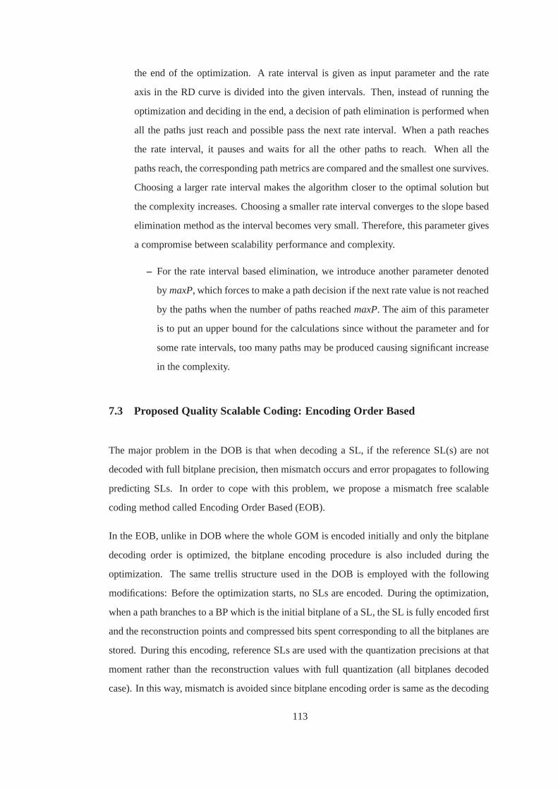
the end of the optimization. A rate interval is given as inputparameter and the rate

axis in the RD curve is divided into the given intervals. Then, instead of running the

optimization and deciding in the end, a decision of path elimination is performed when

all the paths just reach and possible pass the next rate interval. When a path reaches

the rate interval, it pauses and waits for all the other pathsto reach. When all the

paths reach, the corresponding path metrics are compared and the smallest one survives.

Choosing a larger rate interval makes the algorithm closer to the optimal solution but

the complexity increases. Choosing a smaller rate intervalconverges to the slope based

elimination method as the interval becomes very small. Therefore, this parameter gives

a compromise between scalability performance and complexity.

– For the rate interval based elimination, we introduce another parameter denoted

by maxP, which forces to make a path decision if the next rate value isnot reached

by the paths when the number of paths reachedmaxP. The aim of this parameter

is to put an upper bound for the calculations since without the parameter and for

some rate intervals, too many paths may be produced causing significant increase

in the complexity.

7.3 Proposed Quality Scalable Coding: Encoding Order Based

The major problem in the DOB is that when decoding a SL, if the reference SL(s) are not

decoded with full bitplane precision, then mismatch occursand error propagates to following

predicting SLs. In order to cope with this problem, we propose a mismatch free scalable

coding method called Encoding Order Based (EOB).

In the EOB, unlike in DOB where the whole GOM is encoded initially and only the bitplane

decoding order is optimized, the bitplane encoding procedure is also included during the

optimization. The same trellis structure used in the DOB is employed with the following

modifications: Before the optimization starts, no SLs are encoded. During the optimization,

when a path branches to a BP which is the initial bitplane of a SL, the SL is fully encoded first

and the reconstruction points and compressed bits spent corresponding to all the bitplanes are

stored. During this encoding, reference SLs are used with the quantization precisions at that

moment rather than the reconstruction values with full quantization (all bitplanes decoded

case). In this way, mismatch is avoided since bitplane encoding order is same as the decoding

113

order. On the other hand, memory requirement is increased.

The optimization trellis again starts withBP(0, 0, 0). Since initially no SL is encoded, the

SL 0 in GOM frame 0 is encoded first and information of all bitplanes are stored. Again

next possible bitplanes areBP(0, 0, 1), BP(0, 1, 0) andBP(1, 0, 0). if BP(0, 0, 1) is chosen,

since the corresponding SL is encoded before, the stored information for this bitplane is used.

If BP(0, 1, 0) or BP(1, 0, 0) is chosen, since these SLs are not encoded before, first theSL

is encoded and information of all the bitplanes are stored. Note that during the encoding,

these SLs useS L(0, 0) as reference. However, since the reconstruction ofS L(0, 0) with only

BP(0, 0, 0) is used, the mismatch is avoided.

The disadvantage of EOB is that since reference SLs may be used with lower quantization

precisions, the prediction accuracy decreases leading to loss in compression efficiency. On

the other hand, increase in the distortion is much smaller compared to DOB which may face

significant increase in distortion due to the mismatch. Another disadvantage is that during the

optimization, according to different bitplane orderings, encoding of SLs need to be performed

many times. On the other hand, the encoding in DOB is performed only once at the beginning

and the compressed bit values are available during the optimization process.

In summary, the description of the optimization algorithm is as follows:

7.3.1 Rate, Distortion and Path Metrics

In order to achieve the optimal solution, the number of compressed bits for each bitplane

should be used as the rate metric. Since this data change withrespect to the quantization

precisions of reference SLs, the complexity increases compared to DOB due to numerous

encodings. For the distortion metric, the MSE between the decoded GOM and original GOM

brings the optimal solution as in DOB. Again we address approximations of rate and distortion

metrics to decrease complexity as future work.

Having obtained the rate and distortion metrics, the path metric is calculated as the sum of

path metric in the previous state (the area under the RD curveuntil the previous state) and the

resultant area under the RD curve with current branching as in DOB. However, this time when

two paths reach the same state, although they achieve a similar distortion, the rate values may

be different. The reason is that, during the branches and encoding of SLs, the reference SLs

114

Algorithm 2 Quality Scalability Optimization with EOB1: Initialize thepath listwith BP(0, 0, 0)

2: while path list is not emptydo

3: for all Paths in thepath listdo

4: Compute and store rate, distortion and path metric.

5: end for

6: for all Pairs of paths in thepath listdo

7: if Two paths reach the same statethen

8: Remove the one with larger path metric from the list

9: end if

10: end for

11: Eliminate a subset of the paths according to a rule, if exists.

12: if All the paths are at the final statethen

13: break the loop.

14: end if

15: for all Paths remaining in thepath listdo

16: Generate the next possible paths.

17: if There exist next possible pathsthen

18: Remove the current path from the list and update the list withthe newly generated

paths.

19: end if

20: end for

21: end while

22: The survived path in thepath list is the optimal solution.

115

have different quantization levels causing different predictions. As a result, it is not sensible

to compare the path metrics (or areas under RD curves) when two paths reach the same state

since they do not end up at the same RD point. As a solution, we propose to compare the areas

under the RD curves until the smaller rate point. For algorithmic simplifications, similar to

the DOB, slope based elimination and rate interval based elimination are also employed in

EOB.

7.4 Experimental Results

In this section, we evaluate the performances of different methods for scalable coding of

animated meshes. The distortion of the reconstructed modelis calculated with the KG error

and the bitrate is expressed in bits per vertex per frame (bpvf). The results are presented

with operational Rate-Distortion (RD) curves. For the scalable methods to be evaluated, a

full scalable bitstream is obtained for the quantization level Q = 14 and the points on the RD

curves correspond to possible reconstructions when the full bitstream is truncated until that

bitrate value. The RD performance of reference encoder obtained by encoding the model with

quantization levels betweenQ = 8 andQ = 14 are also provided as the ideal performance

desired by the scalable methods. We denote the reference coder by non-scalable in the figures

in the sense that each RD point on the curve correspond to a different bitstream, not a subset

of the bitstream corresponding to the previousQ value. This should not be confused with the

fact the reference encoder is also a scalable coder and we will also provide comparison with

its scalable performance.

7.4.1 Slope Based Optimization

We start the results by first observing the performance of slope based optimization using the

common encoding parametersT = 4 andS = 8. In Figure 7.4, we present comparison

of slope based DOB and EOB with the best performing fixed bitstream ordering policies

(SL->TL->BP, SL->BP->TL, BP->SL->TL). It can be observed that the proposed DOB and

EOB perform significantly better than fixed policies in low and mid bitrates due to the fact

that slope based methods start optimizing from lowest bitrate and chooses the next bitplane

with sharpest slope. In this way initially, a good performance is achieved but as seen from

116

the figure, this does not guarantee a good performance in the high bitrates. However, on the

average, the proposed slope based methods perform significantly better than fixed bitplane

ordering policies.

6 8 10 12 14 16 180

0.5

1

1.5

2

2.5

Bitrate (bpvf)

KG

Err

or (

%)

Cowheavy

SL −> TL −> BitplaneSL −> Bitplane −> TLBitplane −> SL −> TLDOB SlopeEOB SlopeNon scalable

Figure 7.4: Comparison of slope based optimizations with fixed ordering policies

7.4.2 Simple Encoding Parameters - Full Trellis

Next, we continue with simple encoding parameters to evaluate the performance of full trel-

lis structure. The simple encoding parameters consist of number of temporal layers (T)= 2,

number of spatial layers (S)= 2. When larger encoding parameters are used, the simulation

of full trellis takes unmeasurably long time. In Figure 7.5,comparison of full trellis and slope

based approximation is provided for both DOB and EOB. It is observed that all the meth-

ods perform similarly for this specific simple parameters. The slope based methods perform

usually slightly worse and sometimes moderately worse thanfull trellis based methods. In

the rest of the experimental results, we will use the larger encoding parameters (T = 4 and

S = 8) and will not present full trellis results due to considerably high complexity. However,

the results in Figure 7.5 show that it may be possible to achieve results close to the full trellis.

As seen from the previous figures, the slope based methods mayhave problems due to memo-

117

11 12 13 14 15 16 17 18 190

0.2

0.4

0.6

0.8

1

1.2

1.4

1.6

1.8

2

Bitrate (bpvf)

KG

Err

or (

%)

Cowheavy

DOB Full TrellisDOB SlopeEOB Full TrellisEOB SlopeNon scalable

Figure 7.5: Comparison of full trellis and slope based optimization for simple coding param-eters

ryless nature, i.e. the best decision at a branch may not be the best when more branches ahead

are considered together. On the other hand, the full trellisstructure which considers all fea-

sible branching combinations takes unpractically long time. Therefore, we proposed the rate

interval based optimization as a compromise solution whichapplies full trellis optimization

for rate intervals given as a parameter. In the following results, we present the performance

of rate interval based optimization by considering the rateinterval, minP and maxP.

7.4.3 Effect of Rate Intervals

Figure 7.6 shows the comparison of choosing RInt=0.025, 0.050 and 0.100 bpvf for maxP=100

and 700. In the figure, one GOM of the cowheavy model is scalably encoded with DOB opti-

mization. The results indicate that for this set of RInt values, increasing the RInt value brings

minor improvement at the expense significant increase in theoptimization time. Another ob-

servation is that by increasing the RInt value, the resultant RD curves tend to be more close

to being convex, which is a desired property. Note that theseresults correspond to only one

GOM case whereas results obtained by more GOMs provide better performance accuracy as

will be presented in the following results.

118

6 8 10 12 14 16 180

0.2

0.4

0.6

0.8

1

1.2

Bitrate (bpvf)

KG

Err

or (

%)

Cowheavy, DOB

RInt=0.025 MaxP=100RInt=0.050 MaxP=100RInt=0.100 MaxP=100RInt=0.025 MaxP=700RInt=0.050 MaxP=700RInt=0.100 MaxP=700Non scalable

Figure 7.6: Comparison of different RInt and MaxP parameters for the rate interval basedoptimization method.

6 8 10 12 14 16 180

0.5

1

1.5

2

2.5

Bitrate (bpvf)

KG

Err

or (

%)

Cowheavy

SL −> TL −> BitplaneBitplane −> SL −> TLDOB SlopeEOB SlopeDOB RInt=0.050 MaxP=700EOB RInt=0.050 MaxP=700Non scalable

Figure 7.7: Comparison of best fixed ordering policies, slope based and rate interval basedoptimizations.

119

In Figure 7.7, we see a comparison of rate interval based optimization from previous figure

with fixed ordering policies and slope based optimization. The figure shows that rate interval

based methods outperform the other methods significantly. During comparison of slope based

optimization with fixed ordering policies in Figure 7.4, we had observed that fixed policies

performed better at high bitrates. Now we observe that usingmemory during the optimization

by rate interval based optimization, it is possible to achieve better performance at all bitrates.

7.4.4 Comparison of DOB and EOB

In this part, we compare the operational rate distortion performances of the proposed methods

DOB and EOB. The simulations are performed using the first 12 GOMs of the test models

cowheavy, chicken crossingand face. For the DOB and EOB methods, slope based opti-

mization and rate interval based optimization with variousRInt and MaxP combinations are

simulated.

4 6 8 10 12 14 160

1

2

3

4

5

6

7

Bitrate (bpvf)

KG

Err

or (

%)

Cowheavy

DOB SlopeDOB RInt=0.025 maxP=100DOB RInt=0.050 maxP=700EOB SlopeEOB RInt=0.025 maxP=100EOB RInt=0.050 maxP=700Non scalable

Figure 7.8: Comparison of proposed DOB and EOB methods for cowheavy model.

120

1 2 3 4 5 6 70

0.5

1

1.5

2

Bitrate (bpvf)

KG

Err

or (

%)

Chicken crossing


Figure 7.9: Comparison of proposed DOB and EOB methods for chicken crossing model.

2 4 6 8 10 120

0.2

0.4

0.6

0.8

1

1.2

1.4

1.6

1.8

2

Bitrate (bpvf)

KG

Err

or (

%)

Face


Figure 7.10: Comparison of proposed DOB and EOB methods for face model.

The resultant RD curves of the aforementioned combinationsfor the models cowheavy, chicken

121

crossing and face are presented in Figures 7.8, 7.9 and 7.10 respectively. From the figures,

the following are observed:

• Except for the chicken crossing sequence, the rate intervalbased optimization methods

outperform slope based methods significantly. For the chicken crossing sequence, the

performances are quite similar.

• Comparing the results of one GOM and 12 GOMs for the cowheavy sequence, the

performance difference between slope based optimization and rate interval based opti-

mization is more significant for the 12 GOMs case. This is explained by the fact that

the methods may behave differently for different GOMs.

• It can be observed from the figures that adding more memory into the system by in-

creasing the RInt and maxP parameters improve the RD performance by getting closer

to the non-scalable ideal curve and making the curve more convex.

• Comparing the proposed methods DOB and EOB, EOB performs better especially at

lower bitrates due to the fact the mismatch problem of DOB is more severe in low

bitrates.

7.4.5 Complexity Considerations

As mentioned earlier, running the full trellis optimization takes unmeasurably long time and

requires huge memory usage. However, computation of the many paths during the optimiza-

tion by full trellis is redundant since these paths have a very low chance of being the optimal

solution. Therefore, we proposed several approaches to decrease the computation requirement

and rate-distortion results showed that quite acceptable results can be achieved.

In this part, we provide the optimization times of the proposed approached in the encoder.

Note that the optimization is performed in the encoder and the optimization result is em-

bedded in the encoded bitstream. Since the decoder just reads this information and arranges

the bitplane decoding order, there is negligibly small increase in the decoding time which is

approximately same for all the proposed methods.

The optimization times of the proposed methods are given in Table 7.1. The resultant areas

122

Table 7.1: Average optimization time during encoding per GOM in minutes.

Method Opt. time (m) Area Under RD CurveDOB Slope 1.28 52.30EOB Slope 1.95 38.22

DOB RInt=0.025 maxP=100 2.67 45.95EOB RInt=0.025 maxP=100 3.25 35.12DOB RInt=0.050 maxP=700 67.94 9.97EOB RInt=0.050 maxP=700 89.61 8.64

under the RD curves are also presented since the algorithms aim optimize this value. The val-

ues are calculated for number of minutes passed during the optimization process per GOM.

From the table, it can be observed that DOB takes around 30-50% less time than EOB. As

expected, slope based methods take the smallest time. Another observation is that the opti-

mization time can significantly change with respect toRInt andMaxPparameters.

According to the current implementation and processor speeds, in order to achieve significant

rate-distortion improvements with these parameters, optimization times at the order of hours

are required, which may seem very high for some applicationslike the ones requiring real

time compression. However, in many applications, the encoding may be performed offline

and the decoder is required to be fast. For these applications, the proposed methods are suit-

able. In addition, the presented optimization time resultsare for the current implementation,

where more efficient and optimized implementations may be possible. For example, paral-

lel processing with multi-core processors or GPUs may be efficiently utilized in the trellis

structure.

7.4.6 Visual Comparisons

In this part, apart from the objective metrics, we also show visual comparison of proposed

methods and best performing fixed ordering policies. The frames are 4, 6, 7 and 8 of the

cowheavy sequence are reconstructed by adjusting the compressed bitplane to achieve 8 bpvf

and 12 bpvf. The reason behind choosing these frames is that every frame corresponds to a

different temporal layer. Frame 8 is in TL0, frame 4 is TL1, frame 6is in TL2 and frame 7 is

in TL3. The reconstructed frames are illustrated in Figures7.11 and 7.12 for 8 and 12 bpvf

respectively. Note that in the figures, the models are colored according to the errors in the

surface such that red means low error and deviation from red to other colors mean increasing

123

error.

Examining the figures, first of all, the figure for the 12 bpvf case has more red colors com-

pared to 8 bpvf expectedly. When the methods are compared, the results of the objective

comparisons are confirmed. The proposed methods have much smaller errors than fixed or-

dering policies. In addition, the distribution of error among frames are more uniform. In

fixed ordering policies, it is possible to have some frames atvery high quality and some of the

frames at very low quality. The rate interval based methods perform better than slope based

optimization. Comparing DOB and EOB, EOB looks to perform better slightly for some cases

and moderately for some other cases.

124

(a) BP->SL->TL,Fr. 4 (b) BP->SL->TL,Fr. 6 (c) BP->SL->TL,Fr. 7 (d) BP->SL->TL,Fr. 8

(e) SL->TL->BP, Fr. 4 (f) SL->TL->BP, Fr. 6 (g) SL->TL->BP, Fr. 7 (h) SL->TL->BP, Fr. 8

(i) DOB Slope, Fr. 4 (j) DOB Slope, Fr. 6 (k) DOB Slope, Fr. 7 (l) DOB Slope, Fr. 8

(m) EOB Slope, Fr. 4 (n) EOB Slope, Fr. 6 (o) EOB Slope, Fr. 7 (p) EOB Slope, Fr. 8

(q) DOB RateInt=0.025, Fr. 4

(r) DOB RateInt=0.025, Fr. 6

(s) DOB RateInt=0.025, Fr. 7

(t) DOB RateInt=0.025, Fr. 8

(u) EOB RateInt=0.025, Fr. 4

(v) EOB RateInt=0.025, Fr. 6

(w) EOB RateInt=0.025, Fr. 7

(x) EOB RateInt=0.025, Fr. 8

Figure 7.11: Comparison of visual reconstructions of frames 4,6,7,8 for several methods de-coded at 8 bpvf.

125

(a) BP->SL->TL,Fr. 4 (b) BP->SL->TL,Fr. 6 (c) BP->SL->TL,Fr. 7 (d) BP->SL->TL,Fr. 8

(e) SL->TL->BP, Fr. 4 (f) SL->TL->BP, Fr. 6 (g) SL->TL->BP, Fr. 7 (h) SL->TL->BP, Fr. 8

(i) DOB Slope, Fr. 4 (j) DOB Slope, Fr. 6 (k) DOB Slope, Fr. 7 (l) DOB Slope, Fr. 8

(m) EOB Slope, Fr. 4 (n) EOB Slope, Fr. 6 (o) EOB Slope, Fr. 7 (p) EOB Slope, Fr. 8

(q) DOB RateInt=0.025, Fr. 4

(r) DOB RateInt=0.025, Fr. 6

(s) DOB RateInt=0.025, Fr. 7

(t) DOB RateInt=0.025, Fr. 8

(u) EOB RateInt=0.025, Fr. 4

(v) EOB RateInt=0.025, Fr. 6

(w) EOB RateInt=0.025, Fr. 7

(x) EOB RateInt=0.025, Fr. 8

Figure 7.12: Comparison of visual reconstructions of frames 4,6,7,8 for several methods de-coded at 12 bpvf.

126

7.5 Conclusion

In this work, we have developed quality scalability supportfor predictive layered animated

mesh coding structure, which is also a part of the MPEG-4 FAMCstandard. We have in-

troduced two methods to achieve quality scalability by ordering bitplanes, namely DOB and

EOB. We have proposed the usage of a trellis structure for optimal bitplane ordering and

proposed several methods to decrease computational complexity of optimization process.

Experimental results show that compared to quality scalable achieved by fixed layer/bitplane

ordering of reference SPC coder, the proposed DOB and EOB methods achieve rate distortion

curves significantly closer to the desired non-scalable RD curve. For the trellis structure in

the optimization, trade-off between complexity and RD performance can be achieved by the

rate interval based approximation. Comparing DOB and EOB, EOB usually performs better

at lower bitrates due to the fact that EOB avoids mismatch whereas mismatch present at DOB

affects the performance more at lower bitrates. The performance is similar at higher bitrates.

We note that the performance difference is also content dependent. In order to provide basic

comparison of DOB and EOB methods, we measured the optimization time in the encoder

and observed that DOB takes around 30-50% less time since there exists only one encoding

in the DOB optimization. Finally, subjective analysis by visual reconstructions confirmed the

objective results and also indicated that optimized quality scalable coding also provides better

balanced error distribution among frames.

In this work, the area under the RD curve was chosen as the pathmetric during the optimiza-

tion. However, the optimization framework can be modified tosupport different purposes. For

example, the path metric can be modified such that in additionto the RD performance, mini-

mizing the spatial and/or temporal variance are also taken into account. Other visual quality

metrics can also be used in path metrics.

127

CHAPTER 8

CONCLUSION

In this thesis, we studied several aspects of robust transmission of both static and animated

3D meshes. First, we presented our contributions for MDC anderror resilient coding of

static 3D meshes followed by the contributons for the MDC of animated meshes in the next

chapter. Then we introduced improvements for predictive animated mesh coding to improve

compression performance. Finally, we presented two methods for optimal quality scalable

coding for animated meshes. In summary, the following conclusions are drawn:

In the first work, for the MDC of static meshes, the MDSQ based method is an early work

whereas better results are obtained by the other methods we studuied,TM-MDC andFEC.

Both of the methods employ optimization with respect to varying bandwidth and loss rate of

the channel, which is not available in neither the only previous work in the literature [76] nor

the MDSQ based method. Moreover, number of descriptions anddescription sizes can be

adjusted more flexibly inTM-MDCandFEC based methods. ComparingTM-MDC andFEC

based methods, the methods show similar performance in terms of expected distortion. How-

ever,FEC based method has several advantages. While theFEC based method generates one

compressed bitstream during optimization for any number ofdescriptions,TM-MDCneeds to

generate different compressed bitstream to optimize for different total number of descriptions.

Another advantage ofFEC based method is thatTM-MDC needs to include whole coarsest

level geometry in each description, which may cause high redundancy for higher number

of descriptions whereasFEC based method spreads the bitplanes of coarsest level geometry

according to their importances in compressed bitstream.

For the usage of the proposedFEC based method in packet loss resilient streaming of static

meshes, we have presented an extensive analysis of loss resilient coding methods which are

128

based on optimally protecting compressed bitstreams with FEC codes with respect to given

channel bandwidth and packet loss rate constraints. For theCPM based methods, we intro-

duced a general problem definiton with solution and thekS tepparameter to iterate protection

rates with different steps. The experiments indicates that considerable decrease in optimiza-

tion time can be achieved by increasing thekS tepat the expense of very small PSNR degra-

dation. For the PGC based methods, we proposed RD curve modeling which performed very

close to using original RD curve while providing significantdecrease in optimization time.

Comparing the CPM and PGC based methods, experimental results show that PGC methods

achieve approximately 10db better PSNR for all loss rates. This shows that 10dB compres-

sion performance difference between the PGC and CPM is preserved in packet loss resilient

transmission. Apart from the PSNR performance, PGC based methods have an advantage

of flexible packetization due to the embedded structure of the bitstream which needs to be

generated only once for the PGC method. Simulation in scenarios where the optimization

and channel loss rates mismatch shows that when the model encounters a channel with a loss

rate higher than the optimized rate, the performance degradation can be severe. On the other

hand, when the encountered channel loss rate is lower than the optimization rate, the loss in

the performance is not significant. Therefore when the channel conditions are uncertain or

time varying, it is more robust to optimize loss protection with respect to a higher loss rate.

In the second work of MDC of animated meshes work, we analyzedperformance of the three

proposed methods with redundancy-rate-distortion curvesand visual reconstructions. The

experimental results show thatVertex partitioningperforms better at low redundancies for

especially spatially dense models.Temporal subsamplingperforms better at moderate redun-

dancies (corresponding to including at least the spatial base layer in both descriptions) as well

as low redundancies for spatially coarse models. Layer duplication based MDC can achieve

the lowest redundancies with flexible redundancy allocation capability and can be designed

to achieve the smallest variance of reconstruction qualitybetween consecutive frames.

In the third work, we developed prediction improvements forscalable predictive animated

mesh coding. The improvements are based on weighted spatialprediction, weighted temporal

prediction and exploitation of angular relations of triangles between the frames. The methods

we introduced depend on the spatial-temporal layer decomposition structure presented in the

SPC, which is also a part of the MPEG-4 FAMC standard. The experimental results show that

up to 30% bitrate reductions compared to SPC can be achieved with the combination of pro-

129

posed prediction schemes depending on the content and quantization level. The combination

of proposed algorithms also achieve very competitive performance compared to non-scalable

MPEG-4 FAMC coder.

In our final work, we introduced quality scalability supportfor predictive layered animated

mesh coding structure, which is also a part of the MPEG-4 FAMCstandard. We presented

two methods to achieve quality scalability by ordering bitplanes, namely DOB and EOB. We

proposed the usage of a trellis structure for optimal bitplane ordering and proposed several

methods to decrease computational complexity of optimization process. Experimental results

show that compared to quality scalable achieved by fixed layer/bitplane ordering of reference

SPC coder, the DOB and EOB methods achieve rate distortion curves significantly closer

to the desired non-scalable RD curve. For the trellis structure in the optimization, trade-off

between complexity and RD performance can be achieved by therate interval based approxi-

mation. Comparing DOB and EOB, EOB usually performs better at lower bitrates due to the

fact that EOB avoids mismatch whereas mismatch present at DOB affects the performance

more at lower bitrates. The performance is similar at higherbitrates. We note that the per-

formance difference is also content dependent. In order to provide basic comparison of DOB

and EOB methods, we measured the optimization time in the encoder and observed that DOB

takes around 30-50% less time since there exists only one encoding in the DOB optimization.

Finally, subjective analysis by visual reconstructions confirmed the objective results and also

indicated that optimized quality scalable coding also provides better balanced error distribu-

tion among frames.

130

REFERENCES

[1] A. Norkin, M. O. Bici, G. B. Akar, A. Gotchev, and J. Astola, “Wavelet-based multipledescription coding of 3-D geometry,” inVCIP’07, Proc. SPIE, vol. 6508, San-Jose,US, Jan. 2007, pp. 65 082I–1 –65 082I–10.

[2] M. O. Bici and G. Bozdagi Akar, “Multiple description scalar quantization based 3Dmesh coding,” inProc. IEEE Int. Conf. Image Processing, Atlanta, US, Oct. 2006, pp.553–556.

[3] A. Norkin, M. O. Bici, A. Aksay, C. Bilen, A. Gotchev, G. Akar, K. Egiazarian,and J. Astola, “Multiple Description Coding and its Relevance to 3DTV,” Three-Dimensional Television, pp. 371–426, 2008.

[4] M. O. Bici, A. Norkin, G. Bozdagi Akar, A. Gotchev, and J. Astola, “Multiple descrip-tion coding of 3D geometry with forward error correction codes,” in3DTV-ConferenceThe True Vision - Capture, Transmission and Display of 3D Video, Kos, Greece, May2007.

[5] M. O. Bici, A. Norkin, and G. Bozdagi Akar, “Packet loss resilient transmission of 3Dmodels,” inProc. IEEE Int. Conf. Image Processing (ICIP 2007), San Antonio, US,2007.

[6] M. O. Bici and G. B. Akar, “Joint Source-Channel Coding for Error Resilient Trans-mission of Static 3D Models,”Accepted for publication in Turkish Journal of ElectricalEngineering and Computer Sciences.

[7] M. O. Bici, N. Stefanoski, and G. B. Akar, “Vertex partitioning based Multiple Descrip-tion Coding of 3D dynamic meshes,” in3DTV-Conference The True Vision - Capture,Transmission and Display of 3D Video. IEEE, 2009, pp. 1–4.

[8] M. O. Bici and G. B. Akar, “Multiple description coding of3D dynamic meshesbased on temporal subsampling,” inSociety of Photo-Optical Instrumentation Engi-neers (SPIE) Conference Series, vol. 7543, 2010, p. 10.

[9] M. O. Bici and G. B. Akar, “Multiple description coding ofanimated meshes,”SignalProcessing: Image Communication, vol. In Press, Corrected Proof, pp. –, 2010.

[10] ——, “Improved prediction for layered predictive animated mesh compression,” inProc. IEEE Int. Conf. Image Processing (ICIP 2010), Hong Kong, 2010.

[11] ——, “Improved Prediction Methods For Scalable Predictive Animated Mesh Com-pression,”Submitted to Journal of Visual Communication and Image Representation.

[12] ——, “Optimal Quality Scalability for Predictively Coded Animated Meshes,”Submit-ted to IEEE Transactions on Multimedia.

131

[13] V. Goyal, “Multiple description coding: compression meets the network,”IEEE SignalProcessing Mag., vol. 18, pp. 74–93, September 2001.

[14] Y. Wang, A. Reibman, and S. Lin, “Multiple Description Coding for Video Delivery,”Proceedings of the IEEE, vol. 93, no. 1, pp. 57–70, 2005.

[15] Y. Wang, M. Orchard, V. Vaishampayan, and A. Reibman, “Multiple description cod-ing using pairwise correlating transforms,”Image Processing, IEEE Transactions on,vol. 10, no. 3, pp. 351–366, 2001.

[16] R. R. Blahut,Theory and Practice of Error Control Codes. Reading: Addison-Wesley,1983.

[17] P. Alliez and C. Gotsman, “Recent advances in compression of 3D meshes,” inProc.Symposium on Multiresolution in Geometric Modeling, 2003.

[18] J. Peng, C.-S. Kim, and C.-C. J. Kuo, “Technologies for 3D mesh compression: Asurvey,”Journal of Visual Communication and Image Representation, vol. 16, pp. 688–733, Dec. 2005.

[19] A. Khodakovsky, P. Schroder, and W. Sweldens, “Progressive geometry compression,”in Siggraph 2000, Computer Graphics Proceedings, 2000, pp. 271–278.

[20] R. Pajarola and J. Rossignac, “Compressed progressivemeshes,”IEEE Transactionson Visualization and Computer Graphics, vol. 6, no. 1, pp. 79–93, Jan. 2000.

[21] A. Khodakovsky and I. Guskov, “Compression of normal meshes,” inGeometric Mod-eling for Scientific Visualization. Springer-Verlag, 2003.

[22] F. Moran and N. Garcıa, “Comparison of wavelet-basedthree-dimensional model cod-ing techniques,”IEEE Transactions on Circuits and Systems for Video Technology,vol. 14, no. 7, pp. 937–949, July 2004.

[23] S. Lavu, H. Choi, and R. Baraniuk, “Estimation-quantization geometry coding usingnormal meshes,” inDCC ’03: Proceedings of the Conference on Data Compression.Washington, DC, USA: IEEE Computer Society, 2003, p. 362.

[24] F. Payan and M. Antonini, “3D mesh wavelet coding using efficient model-based bitallocation,” 3D Data Processing Visualization and Transmission, 2002. Proceedings.First International Symposium on, pp. 391 – 394, 2002.

[25] K. Kose, A. E. Cetin, U. Gudukbay, and L. Onural, “3Dmodel compressionusing connectivity-guided adaptive wavelet transform built into 2D SPIHT,” J. Vis.Comun. Image Represent., vol. 21, pp. 17–28, January 2010. [Online]. Available:http://dx.doi.org/10.1016/j.jvcir.2009.09.007

[26] F. Moran, P. Gioia, M. Steliaros, M. Bourges-Sevenier, and N. Garcıa, “Subdivisionsurfaces in MPEG-4,” inProc. IEEE ICIP, vol. III, Sept 2002, pp. 5–8.

[27] M. Bourges-Sevenier and E. S. Jang, “An introduction to the MPEG-4 animationframework eXtension,”IEEE Transactions on Circuits and Systems for Video Tech-nology, vol. 14, no. 7, pp. 928–936, July 2004.

132

[28] A. W. F. Lee, W. Sweldens, P. Schroder, L. Cowsar, and D.Dobkin, “MAPS: Multires-olution adaptive parameterization of surfaces,” inProceedings of SIGGRAPH 98, July1998, pp. 95–104.

[29] C. Loop, “Smooth subdivision surfaces based on triangles,” Master’s Thesis, Univ. ofUtah, Dept. of Mathematics, 1987.

[30] N. Dyn, D. Levin, and J. A. Gregory, “A butterfly subdivision scheme for surface in-terpolation with tension control,”ACM Trans. Graph., vol. 9, no. 2, pp. 160–169, Apr.1990.

[31] C. Touma and C. Gotsman, “Triangle mesh compression,” in Proc. Graphics Interface,Vancouver, BC, Canada, Jun. 1998.

[32] A. Said and W. Pearlman, “A new, fast, and efficient image codec based on set parti-tioning in hierarchical trees,”IEEE Trans. Circuits Syst. Video Technol., vol. 6, no. 3,pp. 243–250, June 1996.

[33] J. E. Lengyel, “Compression of time-dependent geometry,” in Proceedings of the 1999symposium on Interactive 3D graphics., 1999, pp. 89–95.

[34] J. Ahn, C. Kim, C. Kuo, and Y. Ho, “Motion-compensated compression of 3D anima-tion models,”Electronics Letters, vol. 37, no. 24, pp. 1445–1446, 2001.

[35] J. Zhang and C. Owen, “Octree-based animated geometry compression,” inData Com-pression Conference, 2004. Proceedings. DCC 2004, 2004, pp. 508–517.

[36] ——, “Octree-based animated geometry compression,”Computers& Graphics,vol. 31, no. 3, pp. 463–479, 2007.

[37] K. Muller, A. Smolic, M. Kautzner, P. Eisert, and T. Wiegand, “Predictive Compressionof Dynamic 3D Meshes,”Image Processing, 2005 IEEE International Conference on,vol. 1, 2005.

[38] K. Muller, A. Smolic, M. Kautzner, P. Eisert, and T. Wiegand, “Rate-distortion-optimized predictive compression of dynamic 3D mesh sequences,”Signal Processing:Image Communication, vol. 21, no. 9, pp. 812–828, 2006.

[39] K. Mamou, T. Zaharia, and F. Preteux, “A skinning approach for dynamic 3d meshcompression,”Computer Animation and Virtual Worlds, vol. 17, no. 3-4, pp. 337–346,2006.

[40] I. Guskov and A. Khodakovsky, “Wavelet compression of parametrically coherentmesh sequences,” inSCA ’04: Proceedings of the 2004 ACM SIGGRAPH/Eurographicssymposium on Computer animation. Aire-la-Ville, Switzerland, Switzerland: Euro-graphics Association, 2004, pp. 183–192.

[41] F. Payan and M. Antonini, “Wavelet-based compression of 3D mesh sequences,”Pro-ceedings of IEEE ACIDCA-ICMI 2005, 2005.

[42] ——, “Temporal wavelet-based compression for 3D animated models,”Computers&Graphics, vol. 31, no. 1, pp. 77–88, 2007.

133

[43] J. Cho, M. Kim, S. Valette, H. Jung, and R. Prost, “3-d dynamic mesh compressionusing wavelet-based multiresolution analysis,” in2006 IEEE International Conferenceon Image Processing, 2006, pp. 529–532.

[44] Y. Boulfani-Cuisinaud and M. Antonini, “Motion-basedgeometry compensation fordwt compression of 3D mesh sequence,” inIEEE International Conference in ImageProcessing (CD-ROM), 2007.

[45] H. Briceno, P. Sander, L. McMillan, S. Gortler, and H. Hoppe, “Geometry videos: Anew representation for 3D animations,” inProceedings of ACM Symposium on Com-puter Animation 2003., 2003, pp. 136–146.

[46] X. Gu, S. J. Gortler, and H. Hoppe, “Geometry images,” inSIGGRAPH ’02: Proceed-ings of the 29th annual conference on Computer graphics and interactive techniques.New York, NY, USA: ACM Press, 2002, pp. 355–361.

[47] K. Mamou, T. Zaharia, and F. Preteux, “Multi-chart geometry video: A compact repre-sentation for 3D animations,” in3D Data Processing, Visualization, and Transmission,Third International Symposium on, 2006, pp. 711–718.

[48] M. Alexa and W. Muller, “Representing Animations by Principal Components,”Com-puter Graphics Forum, vol. 19, no. 3, pp. 411–418, 2000.

[49] Z. Karni and C. Gotsman, “Compression of soft-body animation sequences,”Comput-ers& Graphics, vol. 28, no. 1, pp. 25–34, 2004.

[50] M. Sattler, R. Sarlette, and R. Klein, “Simple and efficient compression of animationsequences,”Proceedings of the 2005 ACM SIGGRAPH/Eurographics symposium onComputer animation, pp. 209–217, 2005.

[51] R. Amjoun, R. Sondershaus, and W. Straßer, “Compression of complex animatedmeshes,”Advances in Computer Graphics, pp. 606–613, 2006.

[52] R. Amjoun and W. Straßer, “Efficient compression of 3-D dynamic mesh sequences,”J. WSCG, 2007.

[53] J. Heu, C. Kim, and S. Lee, “SNR and temporal scalable coding of 3-D mesh se-quences using singular value decomposition,”Journal of Visual Communication andImage Representation, 2009.

[54] J. Rossignac, “Edgebreaker: Connectivity compression for triangle meshes,”IEEETransactions on Visualization and Computer Graphics, vol. 5, no. 1, pp. 47–61, 1999.

[55] L. Vasa and V. Skala, “Coddyac: Connectivity driven dynamic mesh compression,” in3DTV-Conference The True Vision - Capture, Transmission and Display of 3D Video,2007, pp. 1–4.

[56] ——, “Combined compression and simplification of dynamic 3D meshes,”ComputerAnimation and Virtual Worlds, vol. 20, no. 4, pp. 447–456, 2009.

[57] ——, “COBRA: Compression of the Basis for PCA Represented Animations,” inCom-puter Graphics Forum, vol. 28, no. 6. John Wiley & Sons, 2009, pp. 1529–1540.

[58] ——, “Geometry-Driven Local Neighbourhood Based Predictors for Dynamic MeshCompression,” inComputer Graphics Forum. John Wiley & Sons.

134

[59] J. Yang, C. Kim, and S. Lee, “Compression of 3-D trianglemesh sequences basedon vertex-wise motion vector prediction,”Circuits and Systems for Video Technology,IEEE Transactions on, vol. 12, no. 12, pp. 1178–1184, 2002.

[60] L. Ibarria and J. Rossignac, “Dynapack: space-time compression of the 3D anima-tions of triangle meshes with fixed connectivity,”Proceedings of the 2003 ACM SIG-GRAPH/Eurographics symposium on Computer animation, pp. 126–135, 2003.

[61] R. Amjoun and W. Straßer, “Predictive-DCT Coding for 3DMesh Sequences Com-pression,”Journal of Virtual Reality and Broadcasting, vol. 5, no. 6, 2008.

[62] ——, “Single-rate near lossless compression of animated geometry,”Computer-AidedDesign, vol. 41, no. 10, pp. 711–718, 2009.

[63] N. Stefanoski and J. Ostermann, “Connectivity-GuidedPredictive Compression of Dy-namic 3D Meshes,”Image Processing, 2006 IEEE International Conference on, pp.2973–2976, 2006.

[64] N. Stefanoski, X. Liu, P. Klie, and J. Ostermann, “Scalable linear predictive codingof time-consistent 3D mesh sequences,”3DTV-Conference The True Vision - Capture,Transmission and Display of 3D Video, pp. 1–4, 2007.

[65] N. Stefanoski and J. Ostermann, “Spatially and temporally scalable compression ofanimated 3D meshes with MPEG-4/FAMC,” Proceedings of the IEEE InternationalConference on Image Processing, pp. 2696–2699, 2008.

[66] ——, “SPC: Fast and efficient scalable predictive coding of animated meshes,”Com-puter Graphics Forum, vol. 29, pp. 101–116(16), March 2010.

[67] D. Marpe, H. Schwarz, and T. Wiegand, “Context-based adaptive binary arithmeticcoding in the H. 264/AVC video compression standard,”IEEE Transactions on Circuitsand Systems for Video Technology, vol. 13, no. 7, pp. 620–636, 2003.

[68] K. Mamou, T. Zaharia, and F. Preteux, “Famc: The mpeg-4 standard for animated meshcompression,”Image Processing, 2008. ICIP 2008. 15th IEEE InternationalConfer-ence on, pp. 2676–2679, Oct. 2008.

[69] H. Kirchhoffer, D. Marpe, K. Muller, and T. Wiegand, “Context-adaptive binary arith-metic coding for frame-based animated mesh compression,” in 2008 IEEE Interna-tional Conference on Multimedia and Expo, 2008, pp. 341–344.

[70] P. Cignoni, C. Rocchini, and R. Scopigno, “Metro: Measuring error on simplified sur-faces,”Computer Graphics Forum, vol. 17, pp. 167–174, 1998.

[71] C. L. Bajaj, S. Cutchin, V. Pascucci, and G. Zhuang, “Error resilient transmission ofcompressed vrml,”TICAM, The Univ. Texas at Austin, Austin, TX, Tech. Rep., 1998.

[72] Z. Yan, S. Kumar, and C.-C. J. Kuo, “Error resilient coding of 3-D graphic models viaadaptive mesh segmentation,”IEEE Trans. Circuits Syst. Video Technol., vol. 11, pp.860–873, Jul. 2001.

[73] N.-H. Lin, T.-H. Huang, and B.-Y. Chen, “3D model streaming based on jpeg 2000,”IEEE Transactions on Consumer Electronics, vol. 53, no. 1, 2007.

135

[74] “JPEG 2000 image coding system – Part 3: Motion JPEG 2000, ISO/IEC 15444-3:2002,” 2004.

[75] H. Li, M. Li, and B. Prabhakaran, “Middleware for streaming 3D progressive meshesover lossy networks,”ACM Trans. Multimedia Comput. Commun. Appl., vol. 2, no. 4,pp. 282–317, 2006.

[76] P. Jaromersky, X. Wu, Y. Chiang, and N. Memon, “Multiple-description geometry com-pression for networked interactive 3D graphics,” inProc. ICIG’2004, Dec. 2004, pp.468–471.

[77] G. AlRegib, Y. Altunbasak, and J. Rossignac, “An unequal error protection method forprogressively transmitted 3-D models,”IEEE Trans. Multimedia, vol. 7, pp. 766–776,Aug. 2005.

[78] G. AlRegib, Y. Altunbasak, and R. M. Mersereau, “Bit allocation for joint source andchannel coding of progressively compressed 3-D models,”IEEE Transactions on Cir-cuits and Systems for Video Technology, vol. 15, no. 2, pp. 256–268, Feb. 2005.

[79] G. AlRegib, Y. Altunbasak, and J. Rossignac, “Error-resilient transmission of 3-D mod-els,” ACM Trans. on Graphics, vol. 24(2), pp. 182–208, Apr. 2005.

[80] S. Ahmad and R. Hamzaoui, “Optimal error protection of progressively compressed3D meshes,” inProceedings IEEE International Conference on Multimedia and Expo(ICME’06), Jul 2006, pp. 201–204.

[81] V. Vaishampayan, “Design of multiple description scalar quantizers,”IEEE Trans. In-form. Theory, vol. 39, no. 3, pp. 821–834, May 1993.

[82] C. Tian and S. Hemami, “Universal multiple descriptionscalar quantization: analysisand design,”Information Theory, IEEE Transactions on, vol. 50, no. 9, pp. 2089–2102,2004.

[83] A. Bogomjakov and C. Gotsman, “Universal rendering sequences for transparent ver-tex caching of progressive meshes,”Computer Graphics Forum, vol. 21, pp. 137–148,2002.

[84] Z. Karni, A. Bogomjakov, and C. Gotsman, “Efficient compression and rendering ofmulti-resolution meshes,” inProc. IEEE Visualization, Boston, US, Oct. 2002.

[85] E. Riskin, “Optimum bit allocation via generalized BFOS algorithm,” IEEE Trans.Inform. Theory, vol. 37, pp. 400–4002, March 1991.

[86] Y. Charfi, R. Hamzaoui, and D. Saupe, “Model-based real-time progressive transmis-sion of images over noisy channel,” inProc. WCNC’03, New Orleans, LA, Mar. 2003,pp. 347–354.

[87] A. E. Mohr, E. A. Riskin, and R. E. Ladner, “Graceful degradation over packet erasurechannels through forward error correction,”Proceedings of the 1999 Data Compres-sion Conference (DCC), 1999.

[88] A. Mohr, E. Riskin, and R. Ladner, “Approximately optimal assignment for unequalloss protection,” inProc. ICIP’00, 2000, pp. 367–370.

136

[89] R. Puri and K. Ramchandran, “Multiple description source coding using forward errorcorrectioncodes,” inConference Record of the Thirty-Third Asilomar ConferenceonSignals, Systems, and Computers, vol. 1, Oct 1999.

[90] S. Dumitrescu, X. Wu, and Z. Wang, “Globally optimal uneven error-protected packe-tization of scalable code streams,” inDCC ’02: Proceedings of the Conference on DataCompression, Apr. 2002.

[91] V. Stankovic, R. Hamzaoui, and Z. Xiong, “Packet loss protection of embedded datawith fast local search,”Image Processing. 2002. Proceedings. 2002 International Con-ference on, vol. 2, 2002.

[92] S. Dumitrescu and X. Wu, “Globally optimal uneven erasure-protected multi-grouppacketization of scalable codes,” inProceedings IEEE International Conference onMultimedia and Expo (ICME’05), Jul 2005, pp. 900–903.

[93] B. Girod, K. Stuhlmuller, M. Link, and U. Horn, “Packetloss resilient internet videostreaming,”Proceedings of SPIE Visual Communications and Image Processing ’99,pp. 833–844, 1999.

[94] U. Horn, K. Stuhlmuller, M. Link, and B. Girod, “Robustinternet video transmissionbased on scalable coding and unequal error protection,”Image Com., vol. 15, no. 1–29,pp. 77–94, Sep 1999.

[95] S. Varakliotis, S. Hailes, and J. Ostermann, “Optimally smooth error resilient streamingof 3D wireframe animations,”Proceedings of SPIE, vol. 5150, p. 1009, 2004.

[96] A. Reibman, H. Jafarkhani, Y. Wang, M. Orchard, and R. Puri, “Multiple-descriptionvideo coding using motion-compensated temporal prediction,” IEEE Transactions onCircuits and Systems for Video Technology, vol. 12, no. 3, pp. 193–204, 2002.

[97] T. Tillo, M. Grangetto, G. Olmo,et al., “Redundant slice optimal allocation for H. 264multiple description coding,”IEEE Transactions on Circuits and Systems for VideoTechnology, vol. 18, no. 1, pp. 59–70, 2008.

[98] C. Zhu and M. Liu, “Multiple description video coding based on hierarchical B pic-tures,”IEEE Transactions on Circuits and Systems for Video Technology, vol. 19, no. 4,pp. 511–521, 2009.

[99] B. Demir, S. Erturk, and O. Urhan, “Improved quality multiple description 3D meshcoding with optimal filtering,” in2009 16th IEEE International Conference on ImageProcessing (ICIP), 2009, pp. 3541–3544.

[100] O. Sorkine and D. Cohen-Or, “Least-squares meshes,” in Proceedings of Shape Mod-eling International. IEEE Computer Society Press, 2004, pp. 191–199.

[101] A. Viterbi, “Error bounds for convolutional codes andan asymptotically optimum de-coding algorithm,”IEEE Transactions on Information Theory, vol. 13, no. 2, pp. 260–269, 1967.

[102] G. Forney Jr, “The Viterbi algorithm,”Proceedings of the IEEE, vol. 61, no. 3, pp.268–278, 1973.

137

CURRICULUM VITAE

Mehmet Oguz Bici was born in Ankara, Turkey, in 1983. He received the B.S. degree

in Electrical and Electronics Engineering, from Middle East Technical University, Ankara,

Turkey in 2005. Between 2005 and 2010, he worked as a researcher in Multimedia Research

Group of Electrical and Electronics Engineering Department of Middle East Technical Uni-

versity within 3DTV project, Network of Excellence funded by the European Commission 6th

Framework Programme and MOBILE3DTV project, funded by the European Commission

7th Framework Programme. He is currently working as a researcher in Tampere University

of Technology, Department of Signal Processing. His research interests include coding and

transmission of image, video and 3D meshes. His publications are as follows:

Book Chapters

1. A. Norkin, M. O. Bici, A. Aksay, C. Bilen, A. Gotchev, G. Bozdagi Akar, K. Egiazar-

ian, and J.Astola, ”Multiple description coding and its relevance to 3DTV” in Haldun

M. Ozaktas and Levent Onural (Eds.), ”Three-Dimensional Television: Capture, Trans-

mission, and Display.”, Springer, Heidelberg, 2007. In press

Journals

1. M. O. Bici, G. B. Akar, ”Multiple description coding of animated meshes,” Signal Pro-

cessing: Image Communication, In Press, Corrected Proof, Available online 26 October

2010, ISSN 0923-5965, DOI: 10.1016/j.image.2010.10.004.

2. M. O. Bici, A. Norkin, G. B. Akar, ”Joint Source-Channel Coding for Error Resilient

Transmission of Static 3D Models,” Accepted for publication in Turkish Journal of

Electrical Engineering and Computer Sciences

3. M. O. Bici and G. B. Akar, “Improved Prediction Methods ForScalable Predictive

Animated Mesh Compression,”Submitted to Journal of Visual Communication and

Image Representation

138

4. M. O. Bici and G. B. Akar, “Optimal Quality Scalability forPredictively Coded Ani-

mated Meshes,”Submitted to IEEE Transactions on Multimedia.

International Conference Papers

1. M. O. Bici and G. B. Akar, ”Improved Prediction For LayeredPredictive Animated

Mesh Compression,” International Conference on Image Processing, ICIP 2010, Hong

Kong, Sept 2010.

2. M. O. Bici, D. Bugdayci, G. B. Akar, A. Gotchev, ”Mobile 3D Video Broadcast,” In-

ternational Conference on Image Processing, ICIP 2010, Hong Kong, Sept 2010.

3. M. O. Bici and G. B. Akar, ”Multiple description coding of 3D dynamic meshes based

on temporal subsampling,” in Visual Information Processing and Communication, Proc.

SPIE 7543, 75430C (2010), DOI:10.1117/12.839850, San-Jose, US, Jan. 2010

4. A. Aksay, M. O. Bici, D. Bugdayci, A. Tikanmaki, A. Gotchev, G. B. Akar, ”A Study

on the Effect of MPE-FEC for 3D Video Broadcasting over DVB-H,” Mobimedia 2009,

London, UK, Sept’09.

5. M. O. Bici, N. Stefanoski, G. Bozdagi Akar, ”Vertex Partitioning Based Multiple De-

scription Coding of 3D Dynamic Meshes,” in 3DTV Conference 2009, Potsdam, Ger-

many, 2009

6. M. O. Bici, A. Aksay, A. Tikanmaki, A. Gotchev, G. B. Akar, ”Stereo Video Broad-

casting Simulation for DVB-H,” NEM-Summit’08, St Malo, France, Oct. 2008.

7. M. O. Bici, G. Bozdagi Akar, ”Distributed 3D Dynamic Mesh Coding,” in Proc. IEEE

Int. Conf. Image Processing, San Diego, US, Oct. 2008

8. M. O. Bici, A. Norkin, G. Bozdagi Akar, and A. Gotchev, ”Optimized multiple descrip-

tion scalar quantization based 3D mesh coding,” in Workshopon Information Theoretic

Methods in Science and Engineering (WITMSE) 2008, Tampere,Finland, 2008

9. M. O. Bici, A. Norkin, G. Bozdagi Akar, ”Packet Loss Resilient Transmission of 3D

Models,” in Proc. IEEE Int. Conf. Image Processing, San Antonio, US, Sep. 2007

139

10. M. O. Bici, A. Norkin, G. Bozdagi Akar, A. Gotchev, and J. Astola, ”Multiple De-

scription Coding of 3D Geometry With Forward Error Correction Codes,” in 3DTV

Conference 2007, Kos Island, Greece, 2007

11. A. Norkin, M. O. Bici, G. Bozdagi Akar, A. Gotchev, and J. Astola, ”Wavelet-based

multiple description coding of 3-D geometry,” in Visual Communications and Image

Processing 2007. Proceedings of the SPIE, Volume 6508, pp. 65082I, San-Jose, US,

Jan. 2007.

12. M. O. Bici and G. Bozdagi Akar, ”Multiple description scalar quantization based 3D

mesh coding,” in Proc. IEEE Int. Conf. Image Processing, Atlanta, US, Oct. 2006.

13. A. Aksay, M. O. Bici, G. Bozdagi Akar, ”Evaluation of Disparity Map Characteristics

For Stereo Image Coding,” IEEE International Conference onImage Processing, ICIP-

2005, Italy, Sept. 2005.

National Conference Papers

1. D. Bugdayci, M. P. Bici, A. Aksay, M. Demirtas, G. B. Akar, ”Video + Depth based

3D Video Broadcast over DVB-H,” IEEE SIU 2010 (18th NationalSignal Process-

ing and Applications Conference), Diyarbakir, Turkey, Apr’10. (”DVB-H Uzerinden

Video+Derinlik Tabanli 3B Video Yayini”)

2. M. O. Bici, A. Aksay, A. Tikanmaki, A. Gotchev, G. B. Akar, ”Stereo Video Broad-

cast Over DVB-H,” IEEE SIU 2009 (17th National Signal Processing and Applications

Conference), Antalya, Turkey. (”DVB-HUzerinden Stereo Video Yayini”)

3. C. V. Isik, M. O. Bici, A. Aksay, G. Bozdagi Akar, ”Importance of Side Information

Generation for Distributed Video Coding”, IEEE SIU 2008 (16th National Signal Pro-

cessing and Applications Conference), Didim, Turkey. (”Dagitik Video Kodlama icin

Yan Bilginin Onemi”)

4. M. Oguz Bici, Andrey Norkin, G. Bozdagi Akar, ”Multiple Description Coding of 3D

Meshes Based on Forward Error Correction,” IEEE SIU 2007 (15th National Signal

Processing and Applications Conference), Eskisehir, Turkey. (”3B Aglarin Gonderme

Yonunde Hata Duzeltimine Dayali Coklu Anlatim Kodlanmasi”)

140

5. M. Oguz Bici, G. Bozdagi Akar, ”3D Mesh Coding Using Multiple Description Scalar

Quantizers,” IEEE SIU 2006 (14th National Signal Processing and Applications Con-

ference), Antalya, Turkey. (”Coklu Anlatim Skaler Nicemleyiciler ile 3B Ag Kod-

lama”)

6. A. Aksay, M. Oguz Bici, G. Bozdagi Akar, ”Using Disparity Map Compensation For

Stereo Image Coding,” IEEE SIU 2005 (13th National Signal Processing and Appli-

cations Conference), Kayseri, Turkey. (”Stereo Imge Sikistirma Icin Aykirilik Haritasi

Dengelemesi Kullanimi”)

141

etd.lib.metu.edu.tr of the thesis: ROBUST TRANSMISSION OF 3D MODELS submitted by MEHMET OGUZ B˘...

Documents

Transcript of etd.lib.metu.edu.tr of the thesis: ROBUST TRANSMISSION OF 3D MODELS submitted by MEHMET OGUZ B˘...