Testing the assumptions of linear prediction analysis in normal vowels

M. A. LITTLEa)Applied Dynamical Systems Research Group, Oxford Centre for Industrial and Applied Mathematics, Oxford University, UnitedKingdom, littlem@maths.ox.ac.uk, http://www.maths.ox.ac.uk/adsP. E. McSHARRYOxford Centre for Industrial and Applied Mathematics and Engineering Science, Oxford University, United Kingdom

I. M. MOROZApplied Dynamical Systems Research Group, Oxford Centre for Industrial and Applied Mathematics, Oxford University, UnitedKingdomS. J. ROBERTSPattern Analysis Research Group, Engineering Science, Oxford University, United Kingdom

AbstractThis paper develops an improved surrogate data test to show experimental evidence, for all the simple vowels of USEnglish, for both male and female speakers, that Gaussian linear prediction analysis, a ubiquitous technique in currentspeech technologies, cannot be used to extract all the dynamical structure of real speech time series. The test provides robustevidence undermining the validity of these linear techniques, supporting the assumptions of either dynamical nonlinearityand/or non-Gaussianity common to more recent, complex, efforts at dynamical modelling speech time series. However, anadditional �nding is that the classical assumptions cannot be ruled out entirely, and plausible evidence is given to explainthe success of the linear Gaussian theory as a weak approximation to the true, nonlinear/non-Gaussian dynamics. Thissupports the use of appropriate hybrid linear/nonlinear/non-Gaussian modelling. With a calibrated calculation of statisticand particular choice of experimental protocol, some of the known systematic problems of the method of surrogate datatesting are circumvented to obtain results to support the conclusions to a high level of signi�cance.PACS numbers 43.70.Gr (principle), 43.25.Ts, 43.60.Wy

I. IntroductionThis paper develops an improved method of surrogate data testing (a formal hypothesis test), and thereby demonstratesmore reliable experimental evidence that the assumptions of Gaussian linear prediction of speech time series cannot explainall the dynamics of real, normal vowel speech time series. By making a calibrated calculation of the simple non-Gaussianmeasure of time-delayed mutual information (a generalisation of the concept of autocorrelation), while ensuring that the surro-gates contain no detectable non-Gaussianity, Fig. 1 demonstrates that, for simple, stationary, normal vowel time series of acertain length, the null hypothesis of a Gaussian stochastic process is false to a high level of signi�cance.The core of most modern, established speech technology is the classical linear theory of speech production (Fant, 1960),bringing together the well-developed subjects of linear digital signal processing and linear acoustics to process and analysespeech time series. The biophysical, acoustic assumption that the vocal tract can be modelled as a linear resonator leadsnaturally to the use of digital �ltering and linear prediction analysis (Markel and Gray, 1976), techniques that are basedupon classical statistical signal processing, in turn relying upon a cluster of mathematical results from linear systems theoryand Gaussian, ergodic random processes. With these methods, it is possible to separate the vocal tract resonances from thedriving force of the vocal folds during voiced sounds such as vowels (this technique is demonstrated in, for example Wonget al. (1979)).However, the biomechanics of speech cannot be entirely linear (Kubin, 1995). There are several potential sources ofnonlinearity in speech. A list of these should include turbulent gas dynamics (Teager and Teager, 1989), but also nonlinearvocal fold dynamics due to the interaction between nonlinear aerodynamics and the vocal folds (Story, 2002), feedbackbetween vocal tract resonances and the vocal folds (Quatieri, 2002) and nonlinear vocal fold tissue properties (Chan, 2003).This list is certainly not exhaustive. Simpli�ed vocal fold models also show hysteresis (Lucero, 1999), and in pathologicalcases, evidence for nonlinear bifurcations have been observed in experiments on excised larynxes, and nonlinear modelshave replicated these observations (Herzel et al., 1995).More recently, there has been growing interest in applying tools from nonlinear and non-Gaussian time series analysisto speech time series attempting to characterise and exploit these nonlinear/non-Gaussian phenomena (Kubin, 1995). Al-gorithms for �nding fractal dimensions (Maragos and Potamianos, 1999) and Lyapunov exponents (Banbrook et al., 1999)

1

2have both been applied, giving evidence to support the existence of nonlinearities and possibly chaos in speech. Tools thatattempt to capture other nonlinear effects have been developed and applied Maragos et al. (2002). Speech time series havebeen analysed using higher-order statistics such as the bicoherence and bispectrum (Fackrell, 1996), providing evidenceagainst the existence quadratic nonlinearities detectable with third-order statistical moments, although higher-order mo-ments were not investigated. Further, Bayesian Markov chain Monte Carlo methods (Godsill, 1996) have also been used.There have been several attempts to capture nonlinear dynamical structure in speech. Thus, local linear (Mann, 1999), globalpolynomial (Kubin, 1995), regularised radial basis function (Rank, 2003) and neural network (Wu et al., 1994) methods haveall been used to try to build compact models that can regenerate speech time series, with varying degrees of success.There are however, formidable numerical, theoretical and algorithmic problems associated with the calculation of non-linear dynamical quantities such as Lyapunov exponents or attractor dimensions for real speech time series, casting doubtover whether a nonlinear description can be justi�ed by the data (McSharry, 2005). Circumventing some of these dif�cul-ties, the method of surrogate data testing is a formal hypothesis test allowing an estimate of the likelihood that the nullhypothesis of Gaussianity and/or linearity is true.By this method, Tokuda et al. (2001) detected deterministic nonlinear structure in the intercycle dynamics of severalJapanese vowels using a speci�c phase-space nonlinear statistic and spike-and-wave surrogates. Work reported by Miyanoet al. (2000) used the surrogate data test applied to a Japanese vowel from one male and one female speaker using Fouriersurrogates and the same phase-space statistic. In a related work on animal vocalisations, surrogate analysis tests have beencarried out using a globally nonlinear versus linear prediction statistic and Fourier surrogates (Tokuda et al., 2002). Thesestudies report signi�cant evidence of deterministic nonlinear structure. Improving the reliability of these results for speechtime series is the main aim of the present study, since one of the problems with the surrogate data test is that it is easy tospuriously discount the null hypothesis, as discussed in general by Kugiumtzsis (2001) and McSharry et al. (2003). This isbecause any systematic errors inadvertently introduced while carrying out the test cause a bias towards rejection of the nullhypothesis.The organisation of this paper is as follows. Sec. II. motivates the construction of a surrogate data test method withimproved reliability, and Sec. III. explains the statistic used. Sec. IV. details the method used to construct the surrogates,and Sec. V. applies the method to an example of a known, nonlinear dynamical system. Sec. VI. then applies the methodto normal vowels. Finally, Sec. VII. interprets the results obtained, and Sec. VIII. contains a summary and suggestions forfuture work.II. Problems with Surrogate Data Tests Against Gaussian Linearity in SpeechIn the classical linear modelling of speech, as common to most current speech technology (Kleijn and Paliwal, 1995), givenan acoustic speech pressure time series, it is typically formally assumed that, over a short interval in time1, the vocalfold behaviour can be represented as a (short-time) stationary, ergodic, zero-mean, Gaussian random process (Proakis andManolakis, 1996) that acts a driving input to a linear digital �lter, forcing the �lter into resonance. Assuming Gaussianitymakes it possible to use the ef�cient Yule-Walker equations to �nd the linear prediction coef�cients (Proakis and Manolakis,1996). In wider circles this amounts to the use of what is known as a linear AR, or autoregressive process.It is, however, an open question as to whether real speech time series actually do support these assumptions, leading tothe need for a test of the following null hypothesis: that the data has been generated by a (short-time) stationary, ergodic,zero-mean, Gaussian random process driving a linear resonator. The desire is to obtain suf�cient signi�cance that the nullhypothesis can be rejected, achieved by generating an appropriate number of surrogates using the Fourier transformmethod(Schreiber and Schmitz, 2000). Using this method, the surrogates have the same power spectrum (and thus autocorrelation,by the Wiener-Khintchine theorem (Proakis and Manolakis, 1996)), as the original speech time series, yet have only linear,Gaussian statistical dependencies at different time lags (the speci�cs of the particular surrogate data analysis technique usedare discussed further in the next section).There follows a discussion of a number of systematic errors that arise with the use of these techniques that motivate thedevelopment of a more reliable approach.Firstly, there are problems with the use of Fourier surrogates due to periodicity artifacts, as used by Miyano et al. (2000),introduced because only the �nite, cyclic autocorrelation is preserved, not the autocorrelation of theoretically in�nite du-ration (Schreiber and Schmitz, 2000). Similarly, for spike-and-wave surrogates, as used by Tokuda et al. (2001), the cyclicautocorrelation can differ systematically from the original. Discontinuities can also be introduced if the ends and gradientsof each cycle are not matched, so that the high-frequency energy characteristics of the surrogates is different from the origi-nal (Small et al., 2001). Therefore, this could lead to false rejection of the null hypothesis because the nonlinear statistic mightbe sensitive to differences in the cyclic autocorrelation (and hence frequency characteristics), between the original and thesurrogates (Kugiumtzsis, 2001). It is at least necessary to discount this possibility.

1For commercial speech coding standards, typically 20-30ms, which amounts to a maximum of around 480 samples at a sample rate of 16kHz (Kroonand Kleijn, 1995).

3Secondly, each additional free parameter in the algorithm used to calculate the nonlinear statistic increases the likelihoodthat the results of the test will depend upon the choice of these free parameters (Kugiumtzsis, 2001). Since the statistic usedto obtain the results in both the cited studies of Miyano et al. (2000) and Tokuda et al. (2001) requires the choice of severalfree parameters, varying these may produce a different result, leading again to the spurious rejection of the null hypothesis.Discounting this is also necessary, but for the cited statistic the systematic investigation of such a large parameter spaceposes formidable challenges.Thirdly, in the cited studies, the algorithm used to compute the nonlinear statistic is not shown to be insensitive to other,simpler aspects of the time series such as the overall amplitude or mean value (McSharry et al., 2003). Then, for example, ifthe surrogates all have a different amplitude than the original time series, the nonlinear statistic might re�ect this feature aswell rather than just the existence of structure consistent or inconsistent with the null hypothesis. This will nearly alwayslead to the spurious rejection of the null hypothesis, guarding against this possibility is one aim of the present study.Finally, with the cited studies, analytic values of the statistic are not available for some relevant processes, and so cross-checks of the numerical results with known cases cannot be carried out (for example to ensure that the surrogates really doconform to the null hypothesis).Circumventing these pitfalls, this study introduces an improved surrogate test, carrying out several precautions in thepreparation of the original time series and choice of surrogate generation method, and in the choice, and algorithm, forcalculation of the statistic.

III. Choice of StatisticFrom information theory, a particular metric, the two-dimensional time-delayed mutual information (Fraser and Swinney,1986) allows the detection of correlations between different time-lagged samples of the time series that cannot be detectedby linear statistics based upon second-order moments. Thus rejection of the null hypothesis is con�rmation that the timeseries is generated by a Markov process with non-Gaussian transition probabilities. Note that a speci�c example of such aprocess is a purely deterministic nonlinear dynamical system (but rejection of the null hypothesis does not discriminate adeterministic from a stochastic process).An additional merit to this statistic is the known analytic expression of this value for various linear, Gaussian processes,used to cross-check numerical calculations (Palu�s, 1995).For a function, or time series, u(t), the time-delayed mutual information is:

I [u] (�) =1Z

�11Z

�1 p0;� (u; v) ln p0;� (u; v)dudv � 21Z

�1 p0 (u) ln p0 (u) du (1)and by de�ning the time delay operator: D�u (t) = u (t+ �) ; (2)then p0(u) is the probability density of the undelayed time series D0u(t), and p0;� (u; v) is the joint probability density ofD0u(t) with a time-delayed copy D�u(t). Equation (1) is a metric of statistical dependence and so is zero only when thesamples at time lag zero and � are statistically independent, and positive otherwise.For the null hypothesis of a linear, ergodic, zero-mean Gaussian process, with knowledge of the covariance matrix:

C = � �0;0 ��;0�0;� ��;�� ; (3)

where �i;j is the covariance between Diu(t) and Dju(t), the analytic value of the mutual information is given by:IL [u] (�) = 12 ln�0;0 + 12 ln��;� � 12 ln�1 � 12 ln�2; (4)

where �1 and �2 are the eigenvalues of C.For an independent, identically distributed, zero-mean Gaussian process e(t) of variance �2, the mutual information is:I [e] (�) = � 1

2�ln �2��2�+ 1� if �= 0;0 otherwise: (5)

Note that IL[u] = I[e] if there are no linear autocorrelations in a time series of variance �2. Typically, the integralexpression for I[u] is approximated using summations over discrete probabilities of partitions of u (Kantz and Schreiber,1997), precluding the direct comparison between the value of this expression with the analytical expression IL[u] (Palu�s,

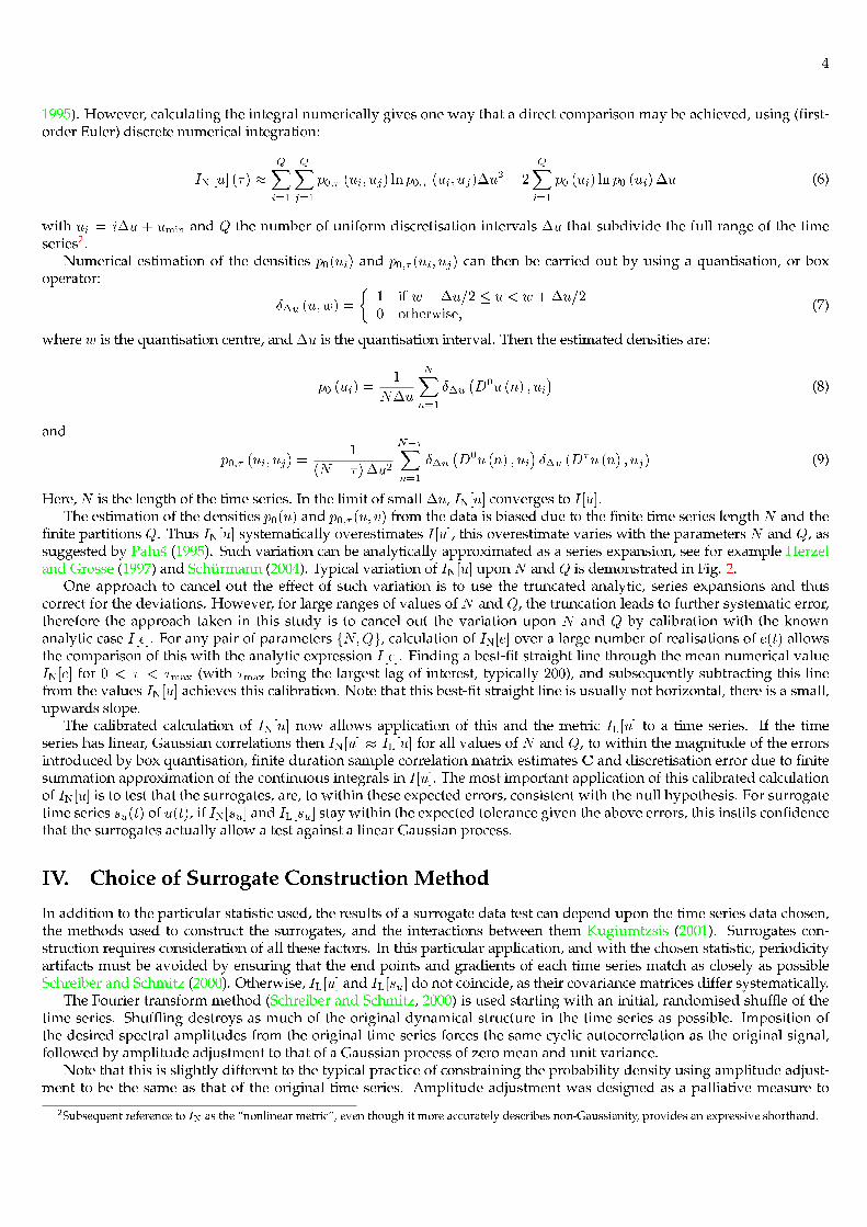
41995). However, calculating the integral numerically gives one way that a direct comparison may be achieved, using (�rst-order Euler) discrete numerical integration:

IN [u] (�) � QXi=1

QXj=1

p0;� (ui; uj) ln p0;� (ui; uj)�u2 � 2 QXi=1

p0 (ui) ln p0 (ui)�u (6)with ui = i�u + umin and Q the number of uniform discretisation intervals �u that subdivide the full range of the timeseries2.Numerical estimation of the densities p0(ui) and p0;� (ui; uj) can then be carried out by using a quantisation, or boxoperator:

��u (u;w) =� 1 if w ��u/2 � u < w +�u/20 otherwise; (7)

where w is the quantisation centre, and�u is the quantisation interval. Then the estimated densities are:p0 (ui) = 1N�u

NXn=1

��u �D0u (n) ; ui� (8)and

p0;� (ui; uj) = 1(N � �)�u2N��Xn=1

��u �D0u (n) ; ui� ��u (D�u (n) ; uj) (9)Here, N is the length of the time series. In the limit of small�u, IN[u] converges to I[u].The estimation of the densities p0(u) and p0;� (u; v) from the data is biased due to the �nite time series length N and the�nite partitions Q. Thus IN[u] systematically overestimates I[u], this overestimate varies with the parameters N and Q, assuggested by Palu�s (1995). Such variation can be analytically approximated as a series expansion, see for example Herzeland Grosse (1997) and Schurmann (2004). Typical variation of IN[u] upon N and Q is demonstrated in Fig. 2.One approach to cancel out the effect of such variation is to use the truncated analytic, series expansions and thuscorrect for the deviations. However, for large ranges of values of N and Q, the truncation leads to further systematic error,therefore the approach taken in this study is to cancel out the variation upon N and Q by calibration with the knownanalytic case I[e]. For any pair of parameters fN;Qg, calculation of IN[e] over a large number of realisations of e(t) allowsthe comparison of this with the analytic expression I[e]. Finding a best-�t straight line through the mean numerical valueIN[e] for 0 < � < �max (with �max being the largest lag of interest, typically 200), and subsequently subtracting this linefrom the values IN[u] achieves this calibration. Note that this best-�t straight line is usually not horizontal, there is a small,upwards slope.The calibrated calculation of IN[u] now allows application of this and the metric IL[u] to a time series. If the timeseries has linear, Gaussian correlations then IN[u] � IL[u] for all values of N and Q, to within the magnitude of the errorsintroduced by box quantisation, �nite duration sample correlation matrix estimates C and discretisation error due to �nitesummation approximation of the continuous integrals in I[u]. The most important application of this calibrated calculationof IN[u] is to test that the surrogates, are, to within these expected errors, consistent with the null hypothesis. For surrogatetime series su(t) of u(t), if IN[su] and IL[su] stay within the expected tolerance given the above errors, this instils con�dencethat the surrogates actually allow a test against a linear Gaussian process.IV. Choice of Surrogate Construction MethodIn addition to the particular statistic used, the results of a surrogate data test can depend upon the time series data chosen,the methods used to construct the surrogates, and the interactions between them Kugiumtzsis (2001). Surrogates con-struction requires consideration of all these factors. In this particular application, and with the chosen statistic, periodicityartifacts must be avoided by ensuring that the end points and gradients of each time series match as closely as possibleSchreiber and Schmitz (2000). Otherwise, IL[u] and IL[su] do not coincide, as their covariance matrices differ systematically.The Fourier transform method (Schreiber and Schmitz, 2000) is used starting with an initial, randomised shuf�e of thetime series. Shuf�ing destroys as much of the original dynamical structure in the time series as possible. Imposition ofthe desired spectral amplitudes from the original time series forces the same cyclic autocorrelation as the original signal,followed by amplitude adjustment to that of a Gaussian process of zero mean and unit variance.Note that this is slightly different to the typical practice of constraining the probability density using amplitude adjust-ment to be the same as that of the original time series. Amplitude adjustment was designed as a palliative measure to

2Subsequent reference to IN as the �nonlinear metric�, even though it more accurately describes non-Gaussianity, provides an expressive shorthand.

5circumvent the problem that certain statistics can vary systematically with the overall amplitude, as discussed earlier. Inthe present study, the nonlinear mutual information calculation is insensitive to the overall amplitude, since the numericalprobability densities are estimated over the full scale of the time series.However, for the present application and choice of statistic, surrogates are required with amplitude distributions con-strained to be the same as a Gaussian process, rather than to be the same as the original time series. This is because thetest is against the null hypothesis of a linear, Gaussian-driven process, using the nonlinear mutual information metric, andfor any Gaussian-driven linear process, the amplitude distribution is also Gaussian (this is a consequence of the fact thatany linear combination of Gaussian processes is also Gaussian). The nonlinear mutual information is of course sensitiveto the entropy of the distribution of the time series, and the original speech time series have a non-Gaussian distribution(this has been demonstrated empirically using various tests, for example, by the use of higher-order statistical moments(Kubin, 1995)). Therefore, surrogates generated by constraining the amplitude distribution to be the same as the original,non-Gaussian speech time series will be inconsistent with the required null hypothesis of this study, and this inconsistencyis then detected by the nonlinear mutual information metric3.For this reason, in practice, constraining the amplitude distribution to be the same as the original, non-Gaussian speechtime series gives, as predicted by theory, a slight, overall increase to the nonlinear mutual information calculation on thesurrogates. Although this is small enough that it does not affect the �nal results, ensuring that theory and practice are inaccord by using amplitude distributions constrained to be Gaussian is of more importance here.Finally, a �nding of this study is no difference to the results with the use of the IAAFT (Iterative Amplitude AdjustedFourier Transform) method (Schreiber and Schmitz, 2000), and so for the sake of computational simplicity this technique isnot used.V. Application to a Toy ExampleHaving described the method, this section demonstrates ruling out the null hypothesis of a linear, stochastic, Gaussianprocess on a toy, deterministic nonlinear example.Figure 3(a) shows, plotted against the discrete time index n = 1; 2 : : : the time series y(n) of an order two, autoregressiveprocess (called an AR(2) process), and Fig. 3(b) the x-coordinate time series x(n) of the Lorenz system, a simple, third-ordernonlinear differential system, for a set of parameters in the chaotic regime. For these two systems, Fig. 4(a) plots both ILand IN for the AR(2) process, demonstrating that the twometrics do indeed agree, showing no signi�cant nonlinearity/non-Gaussianity in this time series. Figure 4(b) plots the same for the Lorenz time series, showing that, after a certain time lag� , the linear and nonlinear metrics begin to diverge signi�cantly and very quickly. This instils con�dence that IL and INbehave as expected. Figure 4(a) shows that the accumulated sources of error in the calibrated calculation of IN amount to asmall discrepancy in the value over all time lags, but that, unlike Fig. 4(b), the two values always track each other to withina certain small amount, as noted by Palu�s (1995)4.In all real-world time series some kind of observation noise must be expected. In order to simulate this, Fig. 5(a) showsthe Lorenz time series corrupted by zero mean Gaussian noise of around 30% of the maximum amplitude.Quanti�cation of the signi�cance of the test is best measured using rank-order statistics, because the form of the dis-tribution of the statistic IN is unknown Schreiber and Schmitz (2000). Requiring a probability of false rejection of the nullhypothesis of P%, generatingM = (0:01P )�1 � 1 surrogates allows the (one-sided) test of the null hypothesis to a signi�-cance level of S = 100% � P%. The probability that IN is largest on the original time series is P% as intended. This studysets a signi�cance level of S = 95%, so that P = 5% and henceM = 19 surrogates are generated, one of which is shown inFig. 5(b).Although familiarity with the Lorenz system might allow detection of the difference by eye, x(n) and sx(n) are verysimilar, and as shown in Fig. 6(a) the linear statistics IL[x] and IL[sx] are practically indistinguishable, and the full extent ofvariation of IL[sx] is very small. Furthermore, Fig. 6(b) shows that the nonlinear metric on the surrogates IN[sx] tracks thelinear metric on the surrogates to within numerical error. Therefore, the surrogates cannot be separated from the originalby the linear metric, and the nonlinear metric on the surrogates agrees with the linear metric on the surrogates. Hencecon�dence is obtained that only linear statistical dependencies are present in the surrogates. Yet, Fig. 6(c) shows that thenonlinear metric on the original IN[x] is larger than the value of this statistic on the surrogates, for most time lags � > 10.This demonstrates that the test is indeed capable of ruling out the null hypothesis for the chaotic system. There areinteresting complications in the details though. For a certain range of low lags (say, � � 10), the results do not warrantcon�dence in rejecting the null hypothesis, because IL and IN on the surrogates differ systematically, noted in Kugiumtzsis(2001).3This is mostly because the entropy features signi�cantly in the calculation of the nonlinear mutual information at all time lags, even if the statisticaldependencies at other time lags could be jointly Gaussian and therefore completely characterised by the autocorrelation.4There is also a small variation in the linear metric since it depends upon the sample covariance matrix estimate from the time series.

6Table I: Vowels and codenames used in this study.

Example Codenamefarther /aa/bird /er/beat /iy/bit /ih/bat /ae/bet /eh/boot /uw/put /uh/pot /ao/but /ah/

VI. Application to Normal VowelsHaving demonstrated that by being selective and avoiding known systematic errors in the use of surrogate data methods,ruling out the null hypothesis where it is indeed known to be false is possible, taking into account the conditions underwhich the test can be said to be valid. The next step is the application of this method to 20 normal, non-pathological voweltime series from the TIMIT database (Fisher et al., 1986) which have been carefully selected to be as short and stationary aspossible. These represent ten different US English sounds from randomly selected male and female speakers, covering allthe principal, simple vowels. Diphthongs are avoided since they are considered to be nonstationary in the sense that thevocal tract resonances are changing with time. All the time series are recorded under quiet acoustic conditions with minimalbackground noise, with 16 bits and sample rate 16kHz. The time series have been normalised to an amplitude range of �1.Table I lists the vowels and their codenames, and Table II lists the TIMIT source audio �le names and lengths in sampleseach time series5. The time series are therefore all approximately 63ms long. Finally, Figs. 7 and 8 shows plots of all the timeseries p(t).Figure 9 picks out one of the time series for closer inspection of the associated surrogates. By eye it is fairly easy toseparate the surrogates from the original. However, for this same vowel, Fig. 10 shows that the linear metric is identical onboth the original time series and the surrogates, and the surrogates are consistent with the null hypothesis as measured bythe nonlinear metric. Therefore the surrogates are consistent with the null hypothesis. Figure 1 shows, again for this samesample vowel, the nonlinear statistic applied to the surrogates and the original speech time series.Figures 11 and 12 show plots comparing the nonlinear metric (calculated with Q = 20) applied to a selection of theoriginal speech time series (IN[p] , thick black line), with the median of the nonlinear metric applied to all correspondingsurrogates (IN[sp], thin, solid black line). The minimum and maximum values of the nonlinear metric for the surrogates areshown (�lled grey area with dotted outlines). Over all the time series and at all time lags 1 � � � 50, there are only twoinstances out of 50� 20 = 1000 time lags where the nonlinear metric on the original time series is not the largest value.VII. DiscussionFigures 11 and 12 show speci�c examples of the result that there are an insigni�cant number of cases where the nonlinearmetric on the original is not the maximum value. Simultaneous cross-checks show that the surrogates are indistinguishableusing second-order statistics, from the original, and, to within the numerical error associated with the computation of thelinear and nonlinear metrics, contain no detectable non-Gaussianity. The broad conclusion is that the linear Gaussian nullhypothesis can be rejected for most lags for all the vowels tested.There are however interesting details that are worth pointing out. It appears that in most cases the nonlinear metricapplied to the speech time series follows the broad peaks and troughs of the mutual information in the surrogates, withsome obvious exceptions. It is the opinion of the authors that this is an indication that the autocorrelation is, to some extent,broadly indicative of the general statistical dependence between samples at speci�c time lags. This is perhaps one of thereasons why Gaussian linear prediction is a useful technique � since it can capture a broad picture of the dynamical structureof the vowel sounds. However, clearly linear prediction cannot represent all the structure.

5Microsoft WAV �les of these time series and software to carry out the calibrated surrogate data test are available from the URL http://www.maths.ox.ac.uk/�littlem/surrogates/.

7Table II: Sound �le sources and sample lengths of time series.

Time series code-name TIMIT �le name Length in samplesfaks0 sx223 aa TEST/DR1/FAKS0/SX223.WAV 1187msjs1 sx369 aa TEST/DR1/MSJS1/SX369.WAV 914fcft0 sa1 er TEST/DR4/FCFT0/SA1.WAV 1106mrws0 si1732 er TRAIN/DR1/MRWS0/SI1732.WAV 948fdac1 si844 iy TEST/DR1/FDAC1/SI844.WAV 1143mreb0 si2005 iy TEST/DR1/MREB0/SI2005.WAV 1148fmaf0 si2089 ih TEST/DR4/FMAF0/SI2089.WAV 1023mbwm0 sa1 ih TEST/DR3/MBWM0/SA1.WAV 1151fjwb1 sa2 ae TRAIN/DR4/FJWB1/SA2.WAV 1280mstf0 sa1 ae TRAIN/DR4/MSTF0/SA1.WAV 1053fdkn0 sx271 eh TRAIN/DR4/FDKN0/SX271.WAV 1261mbml0 si1799 eh TRAIN/DR7/MBML0/SI1799.WAV 1213mdbp0 sx186 uw TRAIN/DR2/MDBP0/SX186.WAV 951fmjb0 si547 uw TRAIN/DR2/FMJB0/SI547.WAV 1036futb0 si1330 uh TEST/DR5/FUTB0/SI1330.WAV 1043mcsh0 sx199 uh TEST/DR3/MCSH0/SX199.WAV 1051fcal1 si773 ao TEST/DR5/FCAL1/SI773.WAV 983mbjk0 si2128 ao TEST/DR2/MBJK0/SI2128.WAV 930fmgd0 sx214 ah TEST/DR6/FMGD0/SX214.WAV 971mdld0 si913 ah TEST/DR2/MDLD0/SI913.WAV 997

A further observation is that this kind of tracking is apparently absent from the comparison between linear and nonlinearmetrics applied to the chaotic Lorenz time series, seen in Fig. 4. Also, as seen in most of the curves in Figs. 11 and 12, forvery small lags (� < 4) the nonlinear and linear metrics mostly coincide and the null hypothesis cannot be comfortablyrejected.One alternative interpretation is that the detected non-Gaussianity is actually spectral nonstationarity in the time series.A deliberate precaution of this study is being careful to select short segments of speech that appear to be as regular aspossible. However, an additional check carried out, that of calculating the power spectral densities at the beginning, middleand end of the time series, shows that the spectral differences are very slight. Even so, some of the vowels are moreirregular than others. Comparing, for example, faks0 sx223 aa against fjwb1 sa2 ae in Figs. 7 and 8, the formermight be considered more stationary than the latter. However, Fig. 11 shows that, even for the apparently stationaryvowel faks0 sx223 aa, the level of non-Gaussianity is signi�cant (and in fact, even more so than the case for vowelfjwb1 sa2 ae, see Fig. 12). In conclusion, therefore, any slight spectral nonstationarity in the vowel time series that couldnot be eradicated is not a signi�cant factor in the detection of non-Gaussianity.VIII. Concluding RemarksThis paper provides evidence, using an improved surrogate data test method, that the linear Gaussian theory of speechproduction cannot be the whole explanation for the dynamical structure of simple vowels. It reaches this conclusion by �rstidentifying (Sec. II.) and circumventing (Secs. III.�IV.) certain systematic problems with the use the surrogate data analysistest method that affect other studies. It demonstrates the effectiveness of the method on a known nonlinear time series (Sec.V.). Application to real speech time series demonstrates that the null hypothesis of Gaussian driven linearity is false, to ahigh level of signi�cance (Sec. VI.).Although the calibrated calculation of IN leads to agreement with IL to within a small discrepancy, more satisfactorywould be to avoid the calibration altogether. To this end, a complete theoretical explanation of the systematic divergenceof this algorithm from the analytic values would be of value, and perhaps also a more sophisticated calculation of IN [u]involving adaptive partitioning and the use of higher-order numerical integration.Careful selection of time series where the linear correlations are stationary over the duration is important, but the du-ration of approximately 60ms is twice as long as the normal frame size used in speech coders. To provide more incentivefor the use of sophisticated nonlinear/non-Gaussian methods in practical speech coding, it might be preferable to test the

8assumptions over shorter time scales. This study �nds that applying the test over such short time scales is problematicfor the calculation of IN since it starts to vary substantially from IL, and con�dence is weakened that the surrogates areconsistent with the null hypothesis. Improvements suggested in the previous paragraph might enable this test to be carriedout.Although this paper avoids spectral nonstationarity, nonstationarity may be measured by many other quantities, suchas running mean, variance and higher-order moments, which could be used as additional checks to assess nonstationarityof non-Gaussian correlations in the speech data Fackrell (1996). This would probably require, however, longer time series,making it harder to �nd natural speech data for which nonstationarity can be avoided.It would also be interesting to apply the same technique to other speech time series, for example consonants whichare supposed to be turbulent yet still amenable to linear prediction analysis Kubin (1995). Diphthongs are supposed to begenerated by nonstationary linear dynamics, but perhaps a nonlinear predictor may model these dynamics more naturally.Application of this test to these vowel sounds might be possible. Pathological speech time series are believed to exhibitsigns of chaos, and this method might be adapted to the detection of such complex dynamics. For whispering and shouting,the dynamics might diverge from linearity further.Finally, these results could have implications in LPAS speech coding standards that rely uponGaussian codebooks Kroonand Kleijn (1995). Although use of linear prediction analysis increases the Gaussianity of the residual with respect to theoriginal speech signal Kubin (1995), this paper suggests that the residual will never be exactly Gaussian. Improvements tothe quality of speech coders may be obtained by appropriate, non-Gaussian codebooks.

9

10 20 30 40 500

0.1

0.2

0.3

0.4

0.5

0.6

t

I(t)

IN

[p] Median I

N[s

p]

Max/Min IN

[sp]

Figure 1: Plot of the nonlinear statistic applied to a particular, sim-ple vowel showing signi�cant discrepancy between the metric ap-plied to linear surrogates (thin black line shows the median value,and the shaded area is bounded by the minimum/maximum val-ues) and the original speech signal (thick black line). The discrep-ancy demonstrates that to a signi�cance level of 95%, there existsshared dynamical information between samples at most time de-lays � that cannot be accounted for by a purely Gaussian, linearmodel. (Vowel codename mbjk0 si2128 ao, see text).

50 100 150 2000

0.1

0.2

0.3

0.4

0.5

0.6

0.7

0.8

t

I N[e

](t)

Q=10, N=1000Q=50, N=1000Q=10, N=2000Q=50, N=2000

Figure 2: Calibrating the nonlinear mutual information metric onan independent, identically distributed, Gaussian process of thesame number of samples N and number of partitions Q of a par-ticular time series. The metric varies systematically with these twoparameters, and hence is adjusted to cancel out this parametric de-pendency.

200 400 600 800 1000-20

-10

0

10

20

200 400 600 800 1000-20

-10

0

10

20

n

AR

(2)

y(n)

(a)

200 400 600 800 1000-20

-10

0

10

20

n

AR

(2)

y(n)

(a)

200 400 600 800 1000-20

-10

0

10

20

n

Lore

nz x

(n)

(b)

Figure 3: Time series of nonlinear versus linear processes: (a) anorder two, Gaussian AR process, (b) the Lorenz system.

10

50 100 150 2000

0.2

0.4

0.6

0.8

1

50 100 150 2000

0.2

0.4

0.6

0.8

1

t

AR

(2)

I(t)

(a) IL[y]

IN

[y]

t

AR

(2)

I(t)

(a) IL[y]

IN

[y]

50 100 150 2000

0.2

0.4

0.6

0.8

1

50 100 150 2000

0.2

0.4

0.6

0.8

1

t

Lore

nz I(

t)

(b) IL[x]

IN

[x]

t

Lore

nz I(

t)

(b) IL[x]

IN

[x]

Figure 4: (a) Linear and nonlinear mutual information metrics co-incide for a purely linear, Gaussian stochastic process, (b) linear andnonlinear mutual information metrics diverge for a nonlinear, de-terministic process. Here Q = 20 and N = 6538.

200 400 600 800 1000-30

-20

-10

0

10

20

30

200 400 600 800 1000-30

-20

-10

0

10

20

30

n

x(n)

(a)

200 400 600 800 1000-30

-20

-10

0

10

20

30

n

x(n)

(a)

200 400 600 800 1000-30

-20

-10

0

10

20

30

n

s x(n)

(b)

Figure 5: (a) Nonlinear Lorenz time series corrupted by Gaussianobservation noise, (b) a suitable, linear stochastic surrogate for theabove.

20 40 60 80 1000

0.2

0.4

0.6

20 40 60 80 1000

0.2

0.4

0.6 (a)

t

I(t)

IL[x]

Median IL[s

x]

Min/Max IL[s

x]

(a)

t

I(t)

IL[x]

Median IL[s

x]

Min/Max IL[s

x]

20 40 60 80 1000

0.2

0.4

0.6

20 40 60 80 1000

0.2

0.4

0.6 (b)

t

I(t)

Median IL[s

x]

Median IN

[sx]

Min/Max IN

[sx]

(b)

t

I(t)

Median IL[s

x]

Median IN

[sx]

Min/Max IN

[sx]

20 40 60 80 1000

0.2

0.4

0.6

20 40 60 80 1000

0.2

0.4

0.6 (c)

t

I(t)

IN

[x] Median I

N[s

x]

Min/Max IN

[sx]

(c)

t

I(t)

IN

[x] Median I

N[s

x]

Min/Max IN

[sx]

Figure 6: Establishing the difference between the Lorenz systemand linear, Gaussian surrogates using cross-application of both lin-ear and nonlinear metrics. (a) Check that surrogates conform to thenull hypothesis. Linear mutual information metric on the surro-gates has a negligible spread of values, and the median linear met-ric over all the surrogates coincides with that of the original timeseries. (b) Check that the nonlinear metric gives the same valuesas the linear metric for the surrogates which have only linear, Gaus-sian statistical dependencies. Themedian of the linear metric on thesurrogates tracks the nonlinear metric on the surrogates to withinnumerical error. (c) Detecting the difference between the determin-istic Lorenz time series and the Gaussian linear surrogates. Thenonlinear metric on the original time series is the largest value ofthe nonlinear metric. Combinedwith the cross-checks in (a) and (b),and given 19 surrogates, the null hypothesis for the Lorenz time se-ries can be ruled out, with a signi�cance level of 95%. Here Q = 20and N = 6358.

11

fdac1_si844_iy mreb0_si2005_iy

fmjb0_si547_uw mdbp0_sx186_uw

fdkn0_sx271_eh mbml0_si1799_eh

fmgd0_sx214_ah mdld0_si913_ah

faks0_sx223_aa msjs1_sx369_aa

Figure 7: Time series of the �rst set of vowels used in this study.The codenames are described in Table II. For clarity, the axes labelshave been removed, the horizontal axis is time index n, the verticalaxis is speech pressure p(n).

fcft0_sa1_er mrws0_si1732_er

fcal1_si773_ao mbjk0_si2128_ao

fjwb1_sa2_ae mstf0_sa1_ae

fmaf0_si2089_ih mbwm0_sa1_ih

futb0_si1330_uh mcsh0_sx199_uh

Figure 8: Time series of the second set of vowels used in this study.The codenames are described in Table II. For clarity, the axes labelshave been removed, the horizontal axis is time index n, the verticalaxis is speech pressure p(n).

12

200 400 600 800-0.5

0

0.5

1

200 400 600 800-0.5

0

0.5

1

n

p(n)

mbjk0_si2128_ao

200 400 600 800

-0.5

0

0.5

n

p(n)

mbjk0_si2128_ao

200 400 600 800

-0.5

0

0.5

s p(n)

n

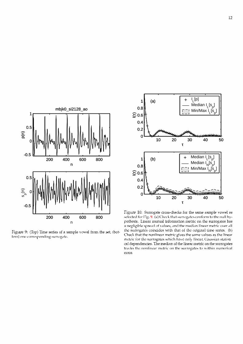
Figure 9: (Top) Time series of a sample vowel from the set, (bot-tom) one corresponding surrogate.

10 20 30 40 500

0.2

0.4

0.6

0.8

1

10 20 30 40 500

0.2

0.4

0.6

0.8

1 (a)

t

I(t)

IL[p]

Median IL[s

p]

Min/Max IL[s

p]

(a)

t

I(t)

IL[p]

Median IL[s

p]

Min/Max IL[s

p]

10 20 30 40 500

0.2

0.4

0.6

0.8

1

10 20 30 40 500

0.2

0.4

0.6

0.8

1 (b)

t

I(t)

Median IL[s

p]

Median IN

[sp]

Min/Max IN

[sp]

(b)

t

I(t)

Median IL[s

p]

Median IN

[sp]

Min/Max IN

[sp]

Figure 10: Surrogate cross-checks for the same sample vowel asselected for Fig. 9. (a) Check that surrogates conform to the null hy-pothesis. Linear mutual information metric on the surrogates hasa negligible spread of values, and the median linear metric over allthe surrogates coincides with that of the original time series. (b)Check that the nonlinear metric gives the same values as the linearmetric for the surrogates which have only linear, Gaussian statisti-cal dependencies. The median of the linear metric on the surrogatestracks the nonlinear metric on the surrogates to within numericalerror.

13

20 400

0.2

0.4

0.6

0.8

20 400

0.2

0.4

0.6

0.8faks0_sx223_aa

20 400

0.2

0.4

0.6

0.8faks0_sx223_aa

20 400

0.2

0.4

0.6

0.8msjs1_sx369_aa

20 400

0.2

0.4

0.6

0.8

msjs1_sx369_aa

20 400

0.2

0.4

0.6

0.8fcft0_sa1_er

20 400

0.2

0.4

0.6

0.8fcft0_sa1_er

20 400

0.2

0.4

0.6

0.8mrws0_si1732_er

Figure 11: Diverging nonlinear mutual information metrics forsimple vowels /aa/ and /er/ and their surrogates. For clarity, theaxes labels have been removed, the horizontal axis is time lag � , thevertical axis is mutual information I(�).

20 400

0.2

0.4

0.6

0.8

20 400

0.2

0.4

0.6

0.8fcal1_si773_ao

20 400

0.2

0.4

0.6

0.8fcal1_si773_ao

20 400

0.2

0.4

0.6

0.8mbjk0_si2128_ao

20 400

0.2

0.4

0.6

0.8

mbjk0_si2128_ao

20 400

0.2

0.4

0.6

0.8fjwb1_sa2_ae

20 400

0.2

0.4

0.6

0.8fjwb1_sa2_ae

20 400

0.2

0.4

0.6

0.8mstf0_sa1_ae

Figure 12: Diverging nonlinear mutual information metrics forsimple vowels /ao/ and /ae/ and their surrogates. For clarity, theaxes labels have been removed, the horizontal axis is time lag � , thevertical axis is mutual information I(�).

14Acknowledgements

Max Little would like to thank Prof. Stephen McLaughlin for helpful discussions about nonlinear speech processing, andReason Machete for interesting insights. He acknowledges the EPSRC, UK for �nancial support.ReferencesM. Banbrook, S. McLaughlin, and I. Mann (1999) �Speech Characterization and Synthesis by Nonlinear Methods� IEEETransactions on Speech and Audio Processing 7(1), pp. 1�17.R. Chan (2003) �Constitutive Characterization of Vocal Fold Viscoelasticity Based on a Modi�ed Arruda-Boyce Eight-ChainModel� J. Acoust. Soc. Am 114(4), pp. 2458�2458.J. Fackrell (1996) �Bispectral Analysis of Speech Signals� Ph.D. thesis; Edinburgh University, UK.G. Fant (1960) Acoustic Theory of Speech Production (Mouton).W. Fisher, G. Doddington, and K. Goudie-Marshall (1986) �The DARPA Speech Recognition Research Database: Speci�ca-tions and Status� in �Proceedings of the DARPAWorkshop on Speech Recognition,� pp. 93�99.A. Fraser and H. Swinney (1986) �Independent Coordinates for Strange Attractors from Mutual Information� PhysicalReview A 33(2), pp. 1134�1140.S. Godsill (1996) �Bayesian Enhancement of Speech and Audio Signals Which Can be Modeled as ARMA Processes� Statist.Rev. 65(1), pp. 1�21.H. Herzel, D. Berry, I. Titze, and I. Steinecke (1995) �Nonlinear Dynamics of the Voice: Signal Analysis and BiomechanicalModeling� Chaos 5(1), pp. 30�35.H. Herzel and I. Grosse (1997) �Correlations in DNA Sequences: The Role of Protein Coding Segments� Phys. Rev. E 55(1),pp. 800�810.H. Kantz and T. Schreiber (1997) Nonlinear Time Series Analysis (Cambridge University Press).W. Kleijn and K. Paliwal (1995) �An Introduction to Speech Coding� in �Speech Coding and Synthesis,� , edited by W. B.Kleijin and K. K. Paliwal (Elsevier Science, Amsterdam); chap. 1; pp. 1�47.P. Kroon and W. Kleijn (1995) �Linear-Prediction based Analysis-by-Synthesis Coding� in �Speech Coding and Synthesis,�, edited by W. B. Kleijin and K. K. Paliwal (Elsevier Science, Amsterdam); chap. 3; pp. 79�119.G. Kubin (1995) �Nonlinear Processing of Speech� in �Speech Coding and Synthesis,� , edited by W. B. Kleijin and K. K.Paliwal (Elsevier Science, Amsterdam); chap. 16; pp. 557�610.D. Kugiumtzsis (2001) �On the Reliability of the Surrogate Data Test for Nonlinearity in the Analysis of Noisy Time Series�Int. J. Bifurcation Chaos Appl. Sci. Eng. 11(7), pp. 1881�1896.J. Lucero (1999) �A Theoretical Study of the Hysteresis Phenomenon at Vocal Fold Oscillation Onset-Offset� J. Acoust. Soc.Am. 105(1), pp. 423�431.I. Mann (1999) �An Investigation of Nonlinear Speech Synthesis and PitchModi�cation Techniques� Ph.D. thesis; EdinburghUniversity, UK.P. Maragos, A. Dimakis, and I. Kokkinos (2002) �Some Advances in Nonlinear Speech Modeling using Modulations, Frac-tals, and Chaos� in �Proceedings of the 14th International Conference on Digital Signal Processing, DSP 2002,� vol. 1; pp.325�332.P. Maragos and A. Potamianos (1999) �Fractal Dimensions of Speech Sounds: Computation and Application to AutomaticSpeech Recognition� J. Acoust. Soc. Am. 105(3), pp. 1925�1932.J. Markel and A. Gray (1976) Linear Prediction of Speech (Springer-Verlag).P. McSharry (2005) �The Danger of Wishing for Chaos� Nonlinear Dynamics, Psychology, and Life Sciences .P. McSharry, L. Smith, and L. Tarassenko (2003) �Prediction of Epileptic Seizures: are Nonlinear Methods Relevant?� NatureMedicine 9(3), pp. 241�242.

15T. Miyano, A. Nagami, I. Tokuda, and K. Aihara (2000) �Detecting Nonlinear Determinism in Voiced Sounds of JapaneseVowel /a/� Int. J. Bifurcation Chaos Appl. Sci. Eng. 10(8), pp. 1973�1979.M. Palu�s (1995) �Testing for Nonlinearity using Redundancies: Quantitative and Qualitative Aspects� Physica D 80(1), pp.186�205.J. Proakis and D. Manolakis (1996) Digital Signal Processing: Principles, Algorithms, and Applications (Prentice-Hall).T. Quatieri (2002) Discrete-Time Speech Signal Processing (Prentice-Hall Signal Processing Series).E. Rank (2003) �Application of Bayesian Trained RBFNetworks to Nonlinear Time-SeriesModeling� Signal Processing 83(7),pp. 1393�1410.T. Schreiber and A. Schmitz (2000) �Surrogate Time Series� Physica D 142(3), pp. 346�382.T. Schurmann (2004) �Bias Analysis in Entropy Estimation� J. Phys. A: Math. Gen. 37, p. 295301.M. Small, D. Yu, and R. Harrison (2001) �Surrogate Test for Pseudoperiodic Time Series Data� Physical Review Letters87(18), pp. 188�101.

B. H. Story (2002) �An Overview of the Physiology, Physics and Modeling of the Sound Source for Vowels� Acoust. Sci. &Tech. 23(4), pp. 195�206.H. M. Teager and S. M. Teager (1989) �Evidence for Nonlinear Sound Production Mechanisms in the Vocal Tract� SpeechProduction and Speech Modelling, NATO Advanced Study Institute Series D 55, pp. 241�261.I. Tokuda, T. Miyano, and K. Aihara (2001) �Surrogate Analysis for Detecting Nonlinear Dynamics in Normal Vowels� J.Acoust. Soc. Am. 110(6), pp. 3207�3217.I. Tokuda, T. Riede, J. Neubauer, M. Owren, and H. Herzel (2002) �Nonlinear Analysis of Irregular Animal Vocalizations� J.Acoust. Soc. Am. 111, pp. 2908�2919.D. Wong, J. Markel, and A. Gray (1979) �Least Squares Glottal Inverse Filtering from the Acoustic Speech Waveform� IEEETransactions on Acoustics, Speech, and Signal Processing 27(4), pp. 350�355.L. Wu, M. Niranjan, and F. Fallside (1994) �Fully Vector Quantized Neural Network-Based Code-Excited Nonlinear Predic-tive Speech Coding� IEEE Transactions on Speech and Audio Processing 2(4), pp. 482�489.