Estimation, prediction and the Stein phenomenon under divergence loss
21
Journal of Multivariate Analysis 99 (2008) 1941–1961 www.elsevier.com/locate/jmva Estimation, prediction and the Stein phenomenon under divergence loss Malay Ghosh * , Victor Mergel, Gauri Sankar Datta Department of Statistics, University of Florida, Gainesville, FL 32611-8545, United States Department of Statistics, University of Georgia, Athens, GA 30602-1952, United States Received 15 March 2007 Available online 8 February 2008 Abstract We consider two problems: (1) estimate a normal mean under a general divergence loss introduced in [S. Amari, Differential geometry of curved exponential families — curvatures and information loss, Ann. Statist. 10 (1982) 357–387] and [N. Cressie, T.R.C. Read, Multinomial goodness-of-fit tests, J. Roy. Statist. Soc. Ser. B. 46 (1984) 440–464] and (2) find a predictive density of a new observation drawn independently of observations sampled from a normal distribution with the same mean but possibly with a different variance under the same loss. The general divergence loss includes as special cases both the Kullback–Leibler and Bhattacharyya–Hellinger losses. The sample mean, which is a Bayes estimator of the population mean under this loss and the improper uniform prior, is shown to be minimax in any arbitrary dimension. A counterpart of this result for predictive density is also proved in any arbitrary dimension. The admissibility of these rules holds in one dimension, and we conjecture that the result is true in two dimensions as well. However, the general Baranchick [A.J. Baranchick, a family of minimax estimators of the mean of a multivariate normal distribution, Ann. Math. Statist. 41 (1970) 642–645] class of estimators, which includes the James–Stein estimator and the Strawderman [W.E. Strawderman, Proper Bayes minimax estimators of the multivariate normal mean, Ann. Math. Statist. 42 (1971) 385–388] class of estimators, dominates the sample mean in three or higher dimensions for the estimation problem. An analogous class of predictive densities is defined and any member of this class is shown to dominate the predictive density corresponding to a uniform prior in three or higher dimensions. For the prediction problem, in the special case of Kullback–Leibler loss, our results complement to a certain extent some of the recent important work of Komaki [F. Komaki, A shrinkage predictive distribution for multivariate normal observations, Biometrika 88 (2001) 859–864] and George, Liang and Xu [E.I. George, F. Liang, X. Xu, Improved minimax predictive densities under Kullbak–Leibler loss, Ann. Statist. 34 (2006) 78–92]. * Corresponding address: Department of Statistics, University of Florida, 103 Griffin-Floyd Hall, P.O. Box 118545, Gainesville, FL 32611-8545, United States. E-mail address: [email protected]fl.edu (M. Ghosh). 0047-259X/$ - see front matter c 2008 Elsevier Inc. All rights reserved. doi:10.1016/j.jmva.2008.02.002
-
Upload
malay-ghosh -
Category
Documents
-
view
215 -
download
3
Transcript of Estimation, prediction and the Stein phenomenon under divergence loss

Journal of Multivariate Analysis 99 (2008) 1941–1961www.elsevier.com/locate/jmva
Estimation, prediction and the Stein phenomenon underdivergence loss
Malay Ghosh∗, Victor Mergel, Gauri Sankar Datta
Department of Statistics, University of Florida, Gainesville, FL 32611-8545, United StatesDepartment of Statistics, University of Georgia, Athens, GA 30602-1952, United States
Received 15 March 2007Available online 8 February 2008
Abstract
We consider two problems: (1) estimate a normal mean under a general divergence loss introducedin [S. Amari, Differential geometry of curved exponential families — curvatures and information loss,Ann. Statist. 10 (1982) 357–387] and [N. Cressie, T.R.C. Read, Multinomial goodness-of-fit tests, J. Roy.Statist. Soc. Ser. B. 46 (1984) 440–464] and (2) find a predictive density of a new observation drawnindependently of observations sampled from a normal distribution with the same mean but possibly witha different variance under the same loss. The general divergence loss includes as special cases both theKullback–Leibler and Bhattacharyya–Hellinger losses. The sample mean, which is a Bayes estimator ofthe population mean under this loss and the improper uniform prior, is shown to be minimax in anyarbitrary dimension. A counterpart of this result for predictive density is also proved in any arbitrarydimension. The admissibility of these rules holds in one dimension, and we conjecture that the result istrue in two dimensions as well. However, the general Baranchick [A.J. Baranchick, a family of minimaxestimators of the mean of a multivariate normal distribution, Ann. Math. Statist. 41 (1970) 642–645] classof estimators, which includes the James–Stein estimator and the Strawderman [W.E. Strawderman, ProperBayes minimax estimators of the multivariate normal mean, Ann. Math. Statist. 42 (1971) 385–388] classof estimators, dominates the sample mean in three or higher dimensions for the estimation problem. Ananalogous class of predictive densities is defined and any member of this class is shown to dominatethe predictive density corresponding to a uniform prior in three or higher dimensions. For the predictionproblem, in the special case of Kullback–Leibler loss, our results complement to a certain extent someof the recent important work of Komaki [F. Komaki, A shrinkage predictive distribution for multivariatenormal observations, Biometrika 88 (2001) 859–864] and George, Liang and Xu [E.I. George, F. Liang,X. Xu, Improved minimax predictive densities under Kullbak–Leibler loss, Ann. Statist. 34 (2006) 78–92].
∗ Corresponding address: Department of Statistics, University of Florida, 103 Griffin-Floyd Hall, P.O. Box 118545,Gainesville, FL 32611-8545, United States.
E-mail address: [email protected] (M. Ghosh).
0047-259X/$ - see front matter c© 2008 Elsevier Inc. All rights reserved.doi:10.1016/j.jmva.2008.02.002

1942 M. Ghosh et al. / Journal of Multivariate Analysis 99 (2008) 1941–1961
While our proposed approach produces a general class of predictive densities (not necessarily Bayes, butnot excluding Bayes predictors) dominating the predictive density under a uniform prior. We show alsothat various modifications of the James–Stein estimator continue to dominate the sample mean, and by theduality of estimation and predictive density results which we will show, similar results continue to hold forthe prediction problem as well.c© 2008 Elsevier Inc. All rights reserved.
AMS 2000 subject classifications: 62C15; 62C20; 62C12
Keywords: Admissibility; Baranchick class; Bhattacharyya–Hellinger loss; Empirical Bayes; Kullback–Leibler loss;Minimaxity
1. Introduction
For estimating the normal mean, the classical estimator, namely the sample mean, meets manyimportant frequentist desiderata. It is the UMVUE, the MLE, and the best equivariant estimatorunder translations of the sample space. Also, Blyth [7] proved minimaxity of this estimator inone dimension for a general class of losses, including but not limited to the squared error loss. Healso proved admissibility of the estimator in one dimension while Stein [26] proved admissibilityin two dimensions.
In his seminal 1956 paper, Stein, came up with the surprising result that the sample mean isan inadmissible estimator of normal population mean in dimensions three or more under squarederror loss. Later James and Stein [21] provided an explicit estimator dominating the sample meanunder the same loss. Subsequently, a very general class of minimax estimators dominating thesample mean was provided by Baranchick [3,4]. Strawderman [25] and Faith [16] provided ageneral class of proper Bayes minimax estimators dominating the sample mean. Brandwein andStrawderman [8] showed that the Baranchick class of estimators dominated the sample mean forspherically symmetric distributions under some stronger conditions than those required in thenormal case.
A trivial extension of the above results is that the sample mean is also a minimax predictorof an observation drawn independently from the same normal distribution under squared errorloss in any arbitrary dimension. Its admissibility continues to hold in one and two dimensions.However, in three and higher dimensions, the sample mean is dominated by the James–Steinpredictor and its variants as mentioned in the previous paragraph.
The original results of Stein have been generalized in a variety of ways. Stein [27] provedadmissibility of the Pitman estimator in one or two dimensions under squared error loss, whileits inadmissibility in three or higher dimensions was proven in James and Stein [21]. Brown [9]proved the inadmissibility of the Pitman estimator under a wide class of losses for three or higherdimensions. Later, Brown [10] provided a necessary and sufficient condition for admissibility ofthe sample mean under losses with bounded risk.
While squared error loss has dominated most of the research related to estimation of themultivariate normal mean, there are other losses which are also of interest. Indeed, as pointed outby Robert [24], often it is natural to use losses which compare directly the densities f (·|θ) andf (·|a), where θ is a true parameter. Robert refers to such losses as “intrinsic losses”.
The two most well-used divergence measures between two distributions are theKullback–Leibler (KL) or the entropy distance and the Bhattacharyya–Hellinger (BH) distance[19,5]. The KL distance has received more prominence in statistics literature than the Hellinger

M. Ghosh et al. / Journal of Multivariate Analysis 99 (2008) 1941–1961 1943
distance. However if X i ∼ N (θi , σ2x ) and independent for i = 1, . . . , p, writing X =
(X1, . . . , X p)T and denoting its pdf by f (x|θ), the KL distance between f (x|θ) and f (x|a)
is given by
Eθ
[log
f (X|θ)
f (X|a)
]=
1
2σ 2x‖θ − a‖
2,
where ‖ · ‖ denotes the Euclidean norm. Hence, point estimation based on the KL loss istantamount to squared error loss for known σ 2
x . The other loss, namely the BH loss is givenby
LBH(θ , a) =12
∫ [f
12 (x|θ) − f
12 (x|a)
]2dx = 1 − exp
{−
1
8σ 2x‖θ − a‖
2}
, (1.1)
where the second equality follows from Lemma 2.2 to be proved later in Section 2. This loss isdifferent from the squared error loss and is not convex.
Both KL and BH losses are special cases of a more general divergence loss considered bymany authors. Among others, we refer to Amari [2] and Cressie and Read [13]. This loss is givenby
Lβ(θ , a) =1 −
∫f 1−β(x|θ) f β(x|a)dx
β(1 − β)=
1 − exp[−
β(1−β)
2σ 2x
‖a − θ‖2]
β(1 − β), (1.2)
which is again a consequence of Lemma 2.2. This above loss is to be interpreted as its limitwhen β → 0 or β → 1. In general, one is primarily interested in the case when β → 0,i.e. LKL(θ , a) = Eθ log fθ (X)
fa(X), namely the KL loss. For β = 1/2, the divergence loss is 4 times the
BH loss given in (1.1). Throughout this article, we will perform the calculations with β ∈ (0, 1),and pass on to the endpoints only in the limit when needed.
Recently Komaki [22] and George, Liang and Xu [18] have considered improved minimaxpredictive densities under KL loss. They have developed various shrinkage versions of predictivedensities which dominate under this loss the Bayes predictive density under the uniform priorfor a future observation conditionally independent of the sampled observations. George et al.[18] have also explored various interesting duality results between multivariate estimation andprediction in the normal problem.
The objective of this paper is to consider simultaneously estimation of the normal mean andpredictive density of a future observation conditionally independent of the sampled observationsunder general divergence loss. In this way, we are able to obtain some unifying results coveringboth estimation and prediction for a wide class of losses including important KL and BH losses.Prediction results for KL loss complement those of Komaki [22] and George et al. [18]. While thepresent results produce a general class of predictors (not necessarily Bayes) dominating normalpredictive density under the uniform prior, Komaki [22] and George et al. [18] considered a classof Bayes predictive densities, and found sufficient conditions under which a similar dominanceholds.
The organization of the remaining sections is as follows. We introduce the problems inSection 2, and prove some general results useful for the rest of the paper. In particular, we provetwo lemmas in this section. Lemma 2.1 provides a general expression (not necessarily restrictedto the normal case) of the predictive density under a general divergence loss, while Lemma 2.2 isused repeatedly for finding closed-form expressions of losses associated with various estimatorsand predictors. In Section 3 of this paper, it is shown that the sample mean is a minimax estimator

1944 M. Ghosh et al. / Journal of Multivariate Analysis 99 (2008) 1941–1961
of the population mean in any arbitrary dimension, and its counterpart, namely, the Bayes (underthe uniform prior) predictive density of a future observation conditionally independent of thesampled ones, is a minimax rule in any arbitrary dimension. The admissibility results for bothestimation and predictive density in one dimension are proved in Section 4. The theorems relatedto inadmissibility of the sample mean for estimating the population mean in dimensions threeor more are stated in Section 5. The inadmissibility of its predictive density counterpart is alsogiven in this section. In particular it is shown that the Baranchick class of estimators dominatesthe sample mean under essentially the same conditions as required under squared error loss.Predictive densitites defined in an analogous fashion also dominate the Bayes predictive densityunder a uniform prior. Proofs of these results are presented in the Appendix.
Section 6 gives a variation of the above results and shows in particular that Lindley’s[23] modification of the James–Stein estimator also dominates the sample mean, and showsextensions of these results to regression problems. Corresponding results for predictive densityare also mentioned. Section 7 contains some remarks regarding possible extensions of our results.Two major theorems, the first one finding an expression for the risk, and the second proving ageneral dominance result, both applicable to estimation as well as prediction are proved in theAppendix.
In view of Brown’s [9] result, inadmissibility of the sample mean under the general divergenceloss is not that surprising, at least for estimation. However, the fact that the Baranchick classof estimators continues to dominate the sample mean under general divergence loss seemsquite interesting. Second, the method of proof showing the dominance of the proposed class ofestimators and predictors is quite non-standard. For squared error loss, proof of dominance eitherrequires application of Stein’s identity or explicit evaluation of the risk based on the properties ofnon-central chisquares. For the prediction problem under KL loss, the basic approach of Georgeet al. involves Stein’s identity and a use of the heat equation. In contrast, our method of proofrequires evaluation of the risk for the Baranchick class of estimators and the analogous class ofpredictors; the final dominance proof follows from an integral inequality which seems to be quitenew. The second interesting feature of our paper is that both estimation and predictive densityresults are unified through two key results, namely Theorems 5.1 and 5.2. The general techniquefor proving these theorems seems to be quite novel in its own right.
Eaton [14] considered admissibility of formal Bayes rules for estimation of boundedmeasurable functions of both the parameters and the data under quadratic loss. He consideredalso a wide class of prediction problems when the loss is a quadratic measure of the distancebetween two distributions. The general divergence loss as considered in this paper also measuresthe distance between two distributions, but it is quite different from the quadratic loss. Moreimportantly, our main focus is to demonstrate the loss robustness of the Baranchick class ofestimators and the corresponding predictors, an emphasis quite different from that of Eaton.
2. Some preliminary results
Let X and Y be conditionally independent given θ with corresponding pdf’s p(x|θ) andp(y|θ). We begin with a general expression for the predictive density of Y based on X underthe divergence loss and a prior pdf π(θ), possibly improper. Under the KL loss and the prior pdfπ(θ), the predictive density of Y is given by
πKL(y|x) =
∫p(y|θ)π(θ |x) dθ ,

M. Ghosh et al. / Journal of Multivariate Analysis 99 (2008) 1941–1961 1945
where π(θ |x) is the posterior of θ based on X = x [1]. The predictive density is proper if and onlyif the posterior pdf is proper. We now provide a similar result based on the general divergenceloss which includes the previous result of Aitchison as a special case when β → 0. This result isalso available in [12] with a somewhat different proof.
Lemma 2.1. Under divergence loss and the prior π , the Bayes predictive density of Y is givenby
πD( y|x) = k1
1−β ( y, x)
/∫k
11−β ( y, x)dy, (2.1)
where k( y, x) =∫
p1−β( y|θ)π(θ |x)dθ .
Proof of Lemma 2.1. Under divergence loss, the posterior risk of predicting p( y|θ), by a pdfp( y|x), is β−1(1 − β)−1 times
1 −
∫ [∫p1−β( y|θ)pβ( y|x)dy
]π(θ |x)dθ
= 1 −
∫pβ( y|x)
{∫p1−β( y|θ)π(θ |x) dθ
}dy
= 1 −
∫k( y, x)pβ( y|x)dy. (2.2)
An application of Holder’s inequality now shows that the integral in (2.2) is maximized at
p( y|x) ∝ k1
1−β ( y, x). Again by the same inequality, the denominator of (2.1) is finite providedthe posterior pdf is proper. This leads to the result noting that πD( y|x) has to be a pdf. �
The next lemma, to be used repeatedly in the sequel, provides an expression for the integral ofthe product of two normal densities each raised to a certain power. A proof of this result is givenin the Appendix.
Lemma 2.2. Let Np(x|µ,Σ ) denote the pdf of a p-variate normal random variable with meanvector µ and positive definite variance–covariance matrix Σ . Then for α1 > 0, α2 > 0,∫
[Np(x|µ1,Σ1)]α1 [Np(x|µ2,Σ2)]
α2 dx
= (2π)p2 (1−α1−α2)|Σ1|
12 (1−α1)|Σ2|
12 (1−α2)|α1Σ2 + α2Σ1|
−12
× exp[−
α1α2
2(µ1 − µ2)
T (α1Σ2 + α2Σ1)−1 (µ1 − µ2)
]. (2.3)
The above results are now used to obtain the Bayes estimator of θ and the Bayesian predictivedensity of a future Y ∼ N (θ , σ 2
y Ip) under the general divergence loss and the N (µ, AIp) priorfor θ . We continue to assume that conditional on θ , X ∼ N (θ , σ 2
x Ip), where σ 2x > 0 is known.
Then we have the following result.
Lemma 2.3. Under the loss given in (1.2), the Bayes estimator of θ is (1 − B)X + Bµ, and theBayes predictive density of Y given X is N ((1 − B)X + Bµ, (σ 2
x (1 − B)(1 − β) + σ 2y )Ip).

1946 M. Ghosh et al. / Journal of Multivariate Analysis 99 (2008) 1941–1961
Proof of Lemma 2.3. The Bayes estimator of θ is obtained by minimizing 1−∫
exp[−β(1−β)
2σ 2x
‖θ
− a‖2]N (θ |(1 − B)X + Bµ, σ 2
x (1 − B)Ip)dθ with respect to a, where B = σ 2x (σ 2
x + A)−1. ByLemma 2.2,∫
exp[−
β(1 − β)
2σ 2x
‖θ − a‖2]
N (θ |(1 − B)X + Bµ, σ 2x (1 − B)Ip)dθ
=
(2πσ 2
x
β(1 − β)
)p/2 ∫N (θ |a, σ 2
x β−1(1 − β)−1Ip)N (θ |(1 − B)X
+ Bµ, σ 2x (1 − B)Ip)dθ ∝ exp
[−
‖a − (1 − B)X − Bµ‖2
2σ 2x (β−1(1 − β)−1 + 1 − B)
](2.4)
which is maximized with respect to a at (1 − B)X + Bµ. Hence, the Bayes estimator of θ underthe N (µ, AIp) prior and the general divergence loss is (1− B)X+ Bµ, the posterior mean. Also,by Lemma 2.2, the Bayes predictive density under the divergence loss is given by
πD( y|X) ∝
[∫N 1−β(θ |y, σ 2
y Ip)N (θ |(1 − B)X + Bµ, σ 2x (1 − B)Ip)dθ
] 11−β
∝ N(
y|(1 − B)X + Bµ,(σ 2
x (1 − B)(1 − β) + σ 2y
)Ip
).
This proves the lemma. �
In the limiting (B → 0) case, i.e. under the uniform prior π(θ) = 1, the Bayes estimator of θ
is X, and the Bayes predictive density of Y is N ( y|X, (σ 2x (1 − β) + σ 2
y )Ip).
We denote by δ0 the plug-in predictive density N (X, σ 2x Ip) of N ( y, σ 2
x Ip), and by δ∗
the corresponding Bayes predictive density (under the uniform prior). The corresponding riskexpressions are given in the following theorem.
Theorem 2.4. Under the divergence loss (1.2),
R(θ , δ0) =1
β(1 − β)
[1 − (σ 2
y )pβ2 (σ 2
x )p(1−β)
2 {(1 − β2)σ 2x + βσ 2
y }−p/2
];
R(θ , δ∗) =1
β(1 − β)
[1 − (σ 2
y )pβ2 ((1 − β)σ 2
x + σ 2y )
−pβ2
].
Proof of Theorem 2.4. From Lemma 2.2 with α1 = 1 − β and α2 = β, the divergence loss forthe plug-in predictive density N (θ , σ 2
x Ip), which we denote by δ0, is
L(θ , δ0) =1
β(1 − β)
[1 −
∫N 1−β( y|θ , σ 2
y Ip)Nβ( y|X, σ 2x Ip) dy
]=
1β(1 − β)
[1 − (σ 2
y )pβ2 (σ 2
x )p(1−β)
2 {(1 − β)σ 2x + βσ 2
y }−p/2
× exp
{−
β(1 − β)‖X − θ‖2
2((1 − β)σ 2x + βσ 2
y )
}]. (2.5)
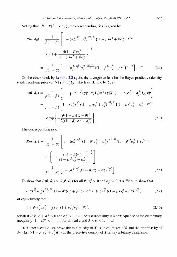
M. Ghosh et al. / Journal of Multivariate Analysis 99 (2008) 1941–1961 1947
Noting that ‖X − θ‖2
∼ σ 2x χ2
p, the corresponding risk is given by
R(θ , δ0) =1
β(1 − β)
1 − (σ 2y )
pβ2 (σ 2
x )p(1−β)
2 {(1 − β)σ 2x + βσ 2
y }−p/2
×
{1 +
β(1 − β)σ 2x
(1 − β)σ 2x + βσ 2
y
}−p2
=1
β(1 − β)
[1 − (σ 2
y )pβ2 (σ 2
x )p(1−β)
2 {(1 − β2)σ 2x + βσ 2
y }−p/2
]. � (2.6)
On the other hand, by Lemma 2.2 again, the divergence loss for the Bayes predictive density(under uniform prior) of N ( y|θ , σ 2
y Ip) which we denote by δ∗ is
L(θ , δ∗) =1
β(1 − β)
[1 −
∫N 1−β( y|θ , σ 2
y Ip)Nβ( y|X, ((1 − β)σ 2x + σ 2
y )Ip) dy]
=1
β(1 − β)
[1 − (σ 2
y )pβ2 ((1 − β)σ 2
x + σ 2y )
p(1−β)2 {(1 − β)2σ 2
x + σ 2y }
−p/2
× exp
{−
β(1 − β)‖X − θ‖2
2((1 − β)2σ 2x + σ 2
y )
}]. (2.7)
The corresponding risk
R(θ , δ∗) =1
β(1 − β)
1 − (σ 2y )
pβ2 ((1 − β)σ 2
x + σ 2y )
p(1−β)2 ((1 − β)2σ 2
x + σ 2y )−
p2
×
{1 +
β(1 − β)σ 2x
(1 − β)2σ 2x + σ 2
y
}−p2
=1
β(1 − β)
[1 − (σ 2
y )pβ2 ((1 − β)σ 2
x + σ 2y )
−pβ2
]. (2.8)
To show that R(θ , δ0) > R(θ , δ∗) for all θ , σ 2x > 0 and σ 2
y > 0, it suffices to show that
(σ 2y )
pβ2 (σ 2
x )p(1−β)
2 {(1 − β2)σ 2x + βσ 2
y }−p/2 < (σ 2
y )pβ2 ((1 − β)σ 2
x + σ 2y )
−pβ2 , (2.9)
or equivalently that
1 + β(σ 2y /σ 2
x − β) > (1 + σ 2y /σ 2
x − β)β , (2.10)
for all 0 < β < 1, σ 2x > 0 and σ 2
y > 0. But the last inequality is a consequence of the elementaryinequality (1 + z)u < 1 + uz for all real z and 0 < u < 1. �
In the next section, we prove the minimaxity of X as an estimator of θ and the minimaxity ofN ( y|X, ((1 − β)σ 2
x + σ 2y )Ip) as the predictive density of Y in any arbitrary dimension.

1948 M. Ghosh et al. / Journal of Multivariate Analysis 99 (2008) 1941–1961
3. Minimaxity results
Suppose X ∼ N (θ , σ 2x Ip), where θ ∈ Rp. By Lemma 2.2 under the general divergence loss
given in (1.2), the risk of X is given by
R(θ , X) =1
β(1 − β)[1 − {1 + β(1 − β)}−p/2
] (3.1)
for all θ . We now prove the minimaxity of X as an estimator of θ .
Theorem 3.1. X is a minimax estimator of the θ in any arbitrary dimension under the divergenceloss given in (1.2).
Proof of Theorem 3.1. Consider the sequence of proper priors N (0, σ 2n Ip) for θ , where σ 2
n −→
∞ as n −→ ∞. We denote this sequence of priors by πn . The Bayes estimator of θ , namely theposterior mean, under the prior πn is
δπn (X) = (1 − Bn)X, (3.2)
with Bn = σ 2x (σ 2
x + σ 2n )−1.
The Bayes risk of δπn under the prior πn is given by:
r(πn, δπn ) =1
β(1 − β)
[1 − E
[exp
{−
β(1 − β)
2σ 2x
‖δπn (X) − θ‖2}]]
, (3.3)
where expectation is taken over the joint distribution of X and θ , with θ having the prior πn .
Since under the prior πn ,
θ |X = x ∼ N(δπn (x), σ 2
x (1 − Bn)Ip
),
it follows that
‖θ − δπn (X)‖2| X = x ∼ σ 2
x (1 − Bn)χ2p,
which does not depend on x. Accordingly, from (3.3),
r(πn, δπn ) =1
β(1 − β)[1 − {1 + β(1 − β)(1 − Bn)}−p/2
]. (3.4)
Since Bn → 0 as n → ∞, it follows from (3.4) that r(πn, δπn ) →1
β(1−β)[1−{1+β(1−β)}−p/2
]
as n → ∞.Noting (3.1), an appeal to a result of Hodges and Lehmann [20] now shows that X is a minimax
estimator of θ for all p. �
Next we prove the minimaxity of the predictive density δ∗(X) = N ( y|X, ((1−β)σ 2x +σ 2
y )Ip)
of Y having pdf N ( y|θ , σ 2y Ip).
Theorem 3.2. δ∗(X) is a minimax predictive density of N ( y|θ , σ 2y Ip) in any arbitrary dimension
under the general divergence loss given in (1.2).
Proof of Theorem 3.2. We have shown already that the predictive density δ∗(X) of
N ( y|θ , σ 2y Ip) has constant risk 1
β(1−β)
[1 − (σ 2
y )pβ2 ((1 − β)σ 2
x + σ 2y )
−pβ2
]under the divergence
loss given in (1.2). Under the same sequence πn of priors considered earlier in this section, by

M. Ghosh et al. / Journal of Multivariate Analysis 99 (2008) 1941–1961 1949
Lemma 2.2, the Bayes predictive density of N ( y|θ , σ 2y Ip) is given by N ( y|(1 − Bn)X, {(1 −
β)(1 − Bn)σ 2x + σ 2
y }Ip). By Lemma 2.2 once again, one gets the identity∫N 1−β( y|θ , σ 2
y Ip)Nβ( y|(1 − Bn)X, {(1 − β)(1 − Bn)σ 2x + σ 2
y }Ip)dy
= (σ 2y )
pβ2 ((1 − β)(1 − Bn)σ 2
x + σ 2y )
p(1−β)2 {(1 − β)2(1 − Bn)σ 2
x + σ 2y }
−p/2
× exp
[−
β(1 − β)‖θ − (1 − Bn)X‖2
2((1 − β)2(1 − Bn)σ 2x + σ 2
y )
]. (3.5)
Noting once again that ‖θ − (1 − Bn)X‖2|X = x ∼ σ 2
x (1 − Bn)χ2p, the posterior risk of δ∗(X)
simplifies to
1β(1 − β)
1 − (σ 2y )
pβ2 ((1 − β)(1 − Bn)σ 2
x + σ 2y )
p(1−β)2
×((1 − β)2(1 − Bn)σ 2x + σ 2
y )−p2
{1 +
β(1 − β)σ 2x (1 − Bn)
(1 − β)2(1 − Bn)σ 2x + σ 2
y
}−p2
=1
β(1 − β)
[1 − (σ 2
y )pβ2 ((1 − β)(1 − Bn)σ 2
x + σ 2y )−
pβ2
]. (3.6)
Since the expression does not depend on x, this is also the same as the Bayes risk of δ∗(X).The Bayes risk converges to
1β(1 − β)
[1 − (σ 2
y )pβ2 ((1 − β)σ 2
x + σ 2y )
−pβ2
].
An appeal to Hodges and Lehmann [20] once again proves the theorem. �
4. Admissibility for p = 1
We use Blyth’s [7] original technique for proving admissibility. First consider the estimationproblem. Suppose that X is not an admissible estimator of θ . Then there exists an estimatorδ0(X) of θ such that R(θ, δ0) ≤ R(θ, X) for all θ with strict inequality for some θ = θ0. Letη = R(θ0, X)− R(θ0, δ0(X)) > 0. Due to continuity of the risk function, there exists an interval[θ0 − ε, θ0 + ε] with ε > 0 such that R(θ, X) − R(θ, δ0(X)) ≥
12η for all θ ∈ [θ0 − ε, θ0 + ε].
Now with the same prior πn(θ) = N (θ |0, σ 2n ),
r(πn, X) − r(πn, δ0(X)) =
∫R[R(θ, X) − R(θ, δ0(X))]πn(dθ)
≥
∫ θ0+ε
θ0−ε
[R(θ, X) − R(θ, δ0(X))]πn(dθ)
≥12η
∫ θ0+ε
θ0−ε
(2πσ 2n )−
12 exp
{−
1
2σ 2n
θ2}
dθ
≥12η(2πσ 2
n )−12
(ε
2
). (4.1)

1950 M. Ghosh et al. / Journal of Multivariate Analysis 99 (2008) 1941–1961
Again,
r(πn, X) − r(πn, δπn (X)) =[{1 + β(1 − β)(1 − Bn)}−1/2
− {1 + β(1 − β)}−1/2]
β(1 − β)
= Oe(Bn) (4.2)
for large n, where Oe denotes the exact order. Since Bn = σ 2x (σ 2
x + σ 2n )−1 and σ 2
n → ∞ asn → ∞, denoting C(> 0) as a generic constant, it follows from (4.1) and (4.2) that for large n,say n ≥ n0,
r(πn, X) − r(πn, δ0(X))
r(πn, X) − r(πn, δπn (X))≥
14η(2π)−1/2σ−1
n C B−1n → ∞ (4.3)
as n → ∞.
Hence, for large n, r(πn, δπn (X)) > r(πn, δ0(X)) which contradicts the Bayesness of δπn (X)
with respect to πn . This proves the admissibility of X for p = 1.
For the prediction problem, suppose there exists a density p(y|ν(X)) which dominatesN (y|X, ((1 − β)σ 2
x + σ 2y )). Since
[((1 − β)(1 − Bn)σ 2x + σ 2
y )−β2 − ((1 − β)σ 2
x + σ 2y )−
β2 ]
β(1 − β)= Oe(Bn)
for large n under the same prior πn , using a similar argument,
r(πn, N (y|X, ((1 − β)σ 2x + σ 2
y ))) − r(πn, p(y|ν(X)))
r(πn, N (y|X, ((1 − β)σ 2x + σ 2
y ))) − r(πn, N (y|X, ((1 − β)(1 − Bn)σ 2x + σ 2
y )))
= O(σ−1n B−1
n ) → ∞, (4.4)
as n → ∞. An argument similar to the previous result now completes the proof. �
Remark 1. The above technique of proving admissibility does not work for p = 2. This isbecause for p = 2, the ratios in the left hand side of (4.3) and (4.4) are greater than or equal tosome constant times σ−2
n B−1n for large n which tends to a constant as n → ∞. We conjecture
the admissibility of X or N ( y|X, ((1 − β)σ 2x + σ 2
y )Ip) for p = 2 under the general divergenceloss for the respective problems of estimation and prediction. It is possible that the technique ofBrown and Fox [11] (see also [17]) can be applied in this context. But that yet remains to beexplored.
5. Inadmissibility results for p ≥ 3
Let S = ‖X‖2/σ 2
x . The Baranchick class of estimators for θ is given by δτ (X) =(1 −
τ(S)S
)X, where one needs some restrictions on τ . The special choice τ(S) = p − 2 (with
p ≥ 3) leads to the James–Stein estimator.It is important to note that the class of estimators δτ (X) can be motivated from an empirical
Bayes (EB) point of view. To see this, we first note that with the N (0, AIp) (A > 0) prior for θ ,the Bayes estimator of θ under the divergence loss is (1 − B)X, where B = σ 2
x (A + σ 2x )−1.
An EB estimator of θ estimates B from the marginal distribution of X. Marginally, X ∼
N (0, σ 2x B−1Ip) so that S is minimal sufficient for B. Thus, a general EB estimator of θ can
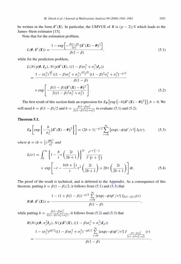
M. Ghosh et al. / Journal of Multivariate Analysis 99 (2008) 1941–1961 1951
be written in the form δτ (X). In particular, the UMVUE of B is (p − 2)/S which leads to theJames–Stein estimator [15].
Note that for the estimation problem,
L(θ , δτ (X)) =
1 − exp[−
β(1−β)
2σ 2x
‖δτ (X) − θ‖2]
β(1 − β), (5.1)
while for the prediction problem,
L(N ( y|θ , Ip), N ( y|δτ (X), ((1 − β)σ 2x + σ 2
y )Ip))
=1 − (σ 2
y )pβ2 ((1 − β)σ 2
x + σ 2y )
p(1−β)2 {(1 − β)2σ 2
x + σ 2y }
−p/2
β(1 − β)
× exp
[−
β(1 − β)‖δτ (X) − θ‖2
2((1 − β)2σ 2x + σ 2
y )
]. (5.2)
The first result of this section finds an expression for Eθ
[exp
{−b‖δτ (X) − θ‖
2}]
, b > 0. We
will need b = β(1 − β)/2 and b =β(1−β)σ 2
x2((1−β)2σ 2
x +σ 2y )
to evaluate (5.1) and (5.2).
Theorem 5.1.
Eθ
[exp
{−
b
σ 2x‖δτ (X) − θ‖
2}]
= (2b + 1)−p/2∞∑
r=0
{exp(−φ)φr/r !
}Ib(r), (5.3)
where φ = (b +12 )
‖θ‖2
σ 2x
and
Ib(r) =
∫∞
0
{1 −
b
tτ
(2t
2b + 1
)}2r tr+p2 −1
Γ(r +
p2
)× exp
[−t −
b(b +12 )
tτ 2(
2t
2b + 1
)+ 2bτ
(2t
2b + 1
)]dt. (5.4)
The proof of the result is technical, and is deferred to the Appendix. As a consequence of thistheorem, putting b = β(1 − β)/2, it follows from (5.1) and (5.3) that
R(θ , δτ (X)) =
1 − (1 + β(1 − β))−p/2∞∑
r=0{exp(−φ)φr/r !} Iβ(1−β)/2(r)
β(1 − β),
while putting b =β(1−β)σ 2
x2((1−β)2σ 2
x +σ 2y )
, it follows from (5.2) and (5.3) that
R(N ( y|θ , σ 2y Ip), N ( y|δτ (X), ((1 − β)σ 2
x + σ 2y )Ip))
=
1 − (σ 2y )pβ/2((1 − β)σ 2
x + σ 2y )−pβ/2
∞∑r=0
{exp(−φ)φr/r !} I β(1−β)σ2x
2((1−β)2σ2x +σ2
y )
(r)
β(1 − β).

1952 M. Ghosh et al. / Journal of Multivariate Analysis 99 (2008) 1941–1961
Hence, proving Ib(r) > 1 for all b > 0 under certain conditions on τ leads to
R(θ , δτ (X)) < R(θ , X)
and
R(N ( y|θ , σ 2y Ip), N ( y|δτ (X), ((1 − β)σ 2
x + σ 2y )Ip))
< R(N ( y|θ , σ 2y Ip), N ( y|X, ((1 − β)σ 2
x + σ 2y )Ip))
for all θ . In the limiting case when β → 0, i.e. for the KL loss, one gets RKL(θ , δτ (X)
)< p/2 =
RKL(θ , X) for all θ , since as shown in Section 1, for estimation, the KL loss is half of the squarederror loss. Similarly, for the prediction problem, as β → 0,
RKL(N ( y|θ , σ 2y Ip), N ( y|δτ (X), ((1 − β)σ 2
x + σ 2y )Ip))
<p
2log
(σ 2
x + σ 2y
σ 2y
)= RKL(N ( y|θ , σ 2
y Ip), N ( y|X, ((1 − β)σ 2x + σ 2
y )Ip))
for all θ .The following theorem provides sufficient conditions on the function τ(·) which guarantee
Ib(r) > 1 for all r = 0, 1, . . . .
Theorem 5.2. Let p ≥ 3. Suppose
(i) 0 < τ(t) < 2(p − 2) for all t > 0;(ii) τ(t) is a differentiable nondecreasing function of t.
Then Ib(r) > 1 for all b > 0.
The proof of Theorem 5.2 is also deferred to Appendix.
Remark 2. Baranchick [3], under squared error loss, proved the dominance of δτ (X) over Xunder (i) and (ii). We may note that the special choice τ(t) = p − 2 for all t leading to theJames–Stein estimator, satisfies both conditions (i) and (ii) of the theorem.
Remark 3. We may note that the Baranchick class of estimators shrinks the sample mean Xtowards 0. Instead one can shrink X towards any arbitrary constant µ. In particular, if weconsider the N (µ, AIp) prior for θ , where µ ∈ Rp is known, then the Bayes estimator of θ
is (1 − B)X + Bµ, where B = σ 2x (A + σ 2
x )−1. A general EB estimator of θ is then given by
δ∗∗(X) =
(1 −
τ(S′)
S′
)X +
τ(S′)
S′µ,
where S′= ‖X − µ‖
2/σ 2x , and Theorem 5.2 with obvious modifications will then provide the
dominance of the EB estimator δ∗∗(X) over X under the divergence loss. The correspondingprediction result is also true.
Remark 4. The special case with τ(t) = c satisfies conditions of the theorem if 0 < c <
2(p − 2). This is the original James–Stein result.
Remark 5. Strawderman [25] considered the hierarchical prior
θ |A ∼ N (0, AIp),

M. Ghosh et al. / Journal of Multivariate Analysis 99 (2008) 1941–1961 1953
where A has pdf
π(A) = δ(1 + A)−1−δ I[A>0]
with δ > 0.
Under the above prior, assuming squared error loss, and recalling that S = ‖X‖2/σ 2
x , the
Bayes estimator of θ is given by(
1 −τ(S)
S
)X, where
τ(t) = p + 2δ −2 exp(− t
2 )∫ 10 λ
p2 +δ−1 exp(−λ
2 t)dλ. (5.5)
Under the general divergence loss, it is not clear whether this estimator is the hierarchical Bayesestimator of θ , although its EB interpretation continues to hold. Besides, as it is well known, thisparticular τ satisfies conditions of Theorem 5.2 if p > 4 + 2δ. Thus the Strawderman class ofestimators dominates X under the general divergence loss. The corresponding predictive densityalso dominates N ( y|X, ((1 − β)σ 2
x + σ 2y )Ip). In a preliminary version of the paper, the authors
proved a weaker result using the increasing failure rate (IFR) property [6] of certain distributions.For the special KL loss, the present results complement those of Komaki [22] and George et al.[18]. The predictive density obtained by these authors under the Strawderman prior, (and Stein’ssuperharmonic prior as a special case) are quite different from the general class of EB predictivedensities of this paper. One of the virtues of the latter is that the expressions are in closed form,and thus it is easy to generate samples from these densities.
6. Lindley’s estimator
Lindley [23] considered a modification of the James–Stein estimator. Rather then shrinkingX towards an arbitrary point, say µ, he proposed shrinking X towards X1p, where X =
p−1∑pi=1 X i and 1p is a p-component column vector with each element equal to 1. Writing
R =∑p
i=1(X i − X)2/σ 2x , Lindley’s estimator is given by
δ(X) = X −p − 3
R(X − X1p), p ≥ 4. (6.1)
The above estimator has a simple EB interpretation. Suppose X|θ ∼ N (θ , σ 2x Ip) and θ has
the Np(µ1p, AIp) prior. Then the Bayes estimator of θ is given by (1− B)X+ Bµ1p where B =
σ 2x (A + σ 2
x )−1. Now if both µ and A are unknown, since marginally X ∼ N (µ1p, σ2x B−1Ip),
(X , R) is complete sufficient for µ and B, and the UMVUE of µ and B−1 are given by X and(p − 3)/R, p ≥ 4.
Following [3] a more general class of EB estimators is given by
δτ∗(X) = X −
τ(R)
R(X − X1p), p ≥ 4. (6.2)
Theorem 6.1. Assume
(i) 0 < τ(t) < 2(p − 3) for all t > 0, p ≥ 4;(ii) τ(t) is a nondecreasing differentiable function of t.
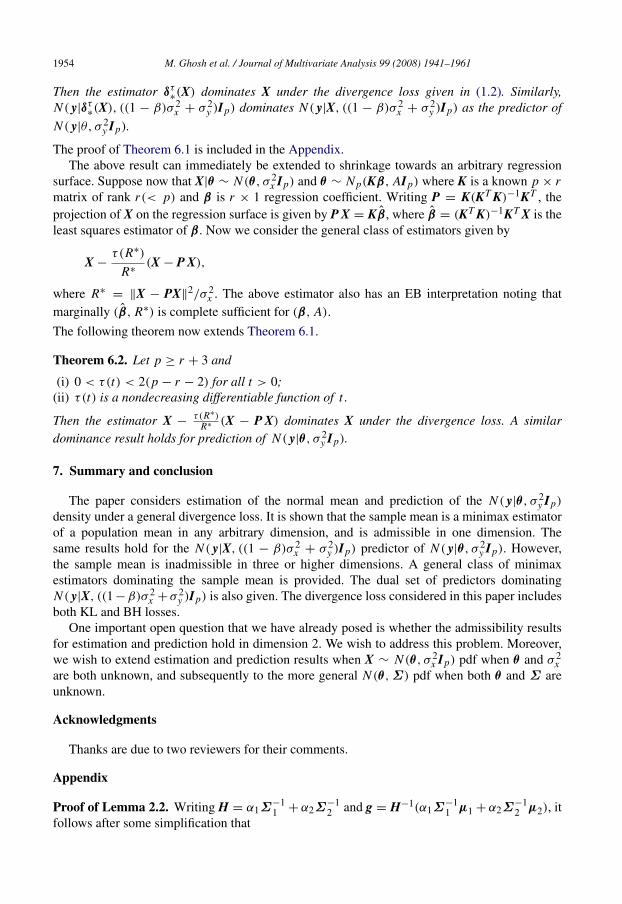
1954 M. Ghosh et al. / Journal of Multivariate Analysis 99 (2008) 1941–1961
Then the estimator δτ∗(X) dominates X under the divergence loss given in (1.2). Similarly,
N ( y|δτ∗(X), ((1 − β)σ 2
x + σ 2y )Ip) dominates N ( y|X, ((1 − β)σ 2
x + σ 2y )Ip) as the predictor of
N ( y|θ, σ 2y Ip).
The proof of Theorem 6.1 is included in the Appendix.The above result can immediately be extended to shrinkage towards an arbitrary regression
surface. Suppose now that X|θ ∼ N (θ , σ 2x Ip) and θ ∼ Np(Kβ, AIp) where K is a known p × r
matrix of rank r(< p) and β is r × 1 regression coefficient. Writing P = K(KT K)−1KT , theprojection of X on the regression surface is given by P X = Kβ, where β = (KT K)−1KT X is theleast squares estimator of β. Now we consider the general class of estimators given by
X −τ(R∗)
R∗(X − P X),
where R∗= ‖X − PX‖
2/σ 2x . The above estimator also has an EB interpretation noting that
marginally (β, R∗) is complete sufficient for (β, A).
The following theorem now extends Theorem 6.1.
Theorem 6.2. Let p ≥ r + 3 and
(i) 0 < τ(t) < 2(p − r − 2) for all t > 0;(ii) τ(t) is a nondecreasing differentiable function of t.
Then the estimator X −τ(R∗)
R∗ (X − P X) dominates X under the divergence loss. A similardominance result holds for prediction of N ( y|θ , σ 2
y Ip).
7. Summary and conclusion
The paper considers estimation of the normal mean and prediction of the N ( y|θ , σ 2y Ip)
density under a general divergence loss. It is shown that the sample mean is a minimax estimatorof a population mean in any arbitrary dimension, and is admissible in one dimension. Thesame results hold for the N ( y|X, ((1 − β)σ 2
x + σ 2y )Ip) predictor of N ( y|θ , σ 2
y Ip). However,the sample mean is inadmissible in three or higher dimensions. A general class of minimaxestimators dominating the sample mean is provided. The dual set of predictors dominatingN ( y|X, ((1 −β)σ 2
x +σ 2y )Ip) is also given. The divergence loss considered in this paper includes
both KL and BH losses.One important open question that we have already posed is whether the admissibility results
for estimation and prediction hold in dimension 2. We wish to address this problem. Moreover,we wish to extend estimation and prediction results when X ∼ N (θ , σ 2
x Ip) pdf when θ and σ 2x
are both unknown, and subsequently to the more general N (θ ,Σ ) pdf when both θ and Σ areunknown.
Acknowledgments
Thanks are due to two reviewers for their comments.
Appendix
Proof of Lemma 2.2. Writing H = α1Σ−11 + α2Σ
−12 and g = H−1(α1Σ
−11 µ1 + α2Σ
−12 µ2), it
follows after some simplification that

M. Ghosh et al. / Journal of Multivariate Analysis 99 (2008) 1941–1961 1955∫[Np(x|µ1,Σ1)]
α1 [Np(x|µ2,Σ2)]α2 dx
= (2π)−p2 (α1+α2)|Σ1|
−12 α1 |Σ2|
−12 α2
∫exp
[−
12(x − g)T H(x − g)
−12
{α1(µ
T1 Σ−1
1 µ1) + α2(µT2 Σ−1
2 µ2) − gT Hg}]
dx
= (2π)p2 (1−α1−α2)|Σ1|
−12 α1 |Σ2|
−12 α2 |H|
−12
× exp[−
12
{α1(µ
T1 Σ−1
1 µ1) + α2(µT2 Σ−1
2 µ2) − gT Hg}]
. (A.1)
It can be checked that
α1(µT1 Σ−1
1 µ1) + α2(µT2 Σ−1
2 µ2) − gT Hg
= α1α2(µ1 − µ2)T (α1Σ2 + α2Σ1)
−1(µ1 − µ2), (A.2)
and
|H|−1/2
= |Σ1|1/2
|Σ2|1/2
|α1Σ2 + α2Σ1|−1/2. (A.3)
Then by (A.2) and (A.3),
right hand side of (A.1) = (2π)p(1−α1−α2)/2|Σ1|
(1−α1)/2|Σ2|
(1−α2)/2|α1Σ2 + α2Σ1|
−1/2
× exp[−
α1α2
2(µ1 − µ2)
T (α1Σ2 + α2Σ1)−1(µ1 − µ2)
].
This proves the lemma. �
Proof of Theorem 5.1. Recall that S = ‖X‖2/σ 2
x . For ‖θ‖ = 0, proof is straightforward. So we
consider ‖θ‖ > 0. Let Z = X/σx and η = θ/σx . First we reexpress 1σ 2
x
∥∥∥(1 −τ(S)
S
)X − θ
∥∥∥2as
∥∥∥∥(1 −τ(‖Z‖
2)
‖Z‖2
)Z − η
∥∥∥∥2
= S +τ 2(S)
S− 2τ(S) + ‖η‖
2− 2ηT Z
(1 −
τ(S)
S
). (A.4)
We begin with the orthogonal transformation Y = CZ where C is an orthogonal matrix withits first row given by (θ1/‖θ‖, . . . , θp/‖θ‖). Writing Y = (Y1, . . . , Yp)
T , the right hand side of(A.4) can be written as
S +τ 2(S)
S− 2τ(S) + ‖η‖
2− 2‖η‖Y1
(1 −
τ(S)
S
), (A.5)
where S = ‖Y‖2. Also we note that Y1, . . . , Yp are mutually independent with Y1 ∼ N (‖η‖, 1),
and Y2, . . . , Yp are iid N (0, 1). Now writing Z =∑p
i=2 Y 2i ∼ χ2
p−1 we have
E
[exp
{−
b
σ 2x‖δτ (X) − θ‖
2}]
=
∫+∞
0
∫+∞
−∞
exp
[−b
{y2
1 + z +τ 2(y2
1 + z)
(y21 + z)
− 2τ(y21 + z) + ‖η‖
2− 2‖η‖y1
×
(1 −
τ(y21 + z)
y21 + z
)}]

1956 M. Ghosh et al. / Journal of Multivariate Analysis 99 (2008) 1941–1961
× (2π)−1/2 exp{−
12(y1 − ‖η‖)2
}exp
{−
12
z
}z
12 (p−1)−1
2p−1
2 Γ(
p−12
) dy1 dz
=
∫+∞
0
∫+∞
−∞
(2π)−1/2 exp
[−
(b +
12
)(y1 − ‖η‖)2
−bτ 2(y2
1 + z)
(y21 + z)
+ 2bτ(y21 + z) − 2b‖η‖y1
τ(y21 + z)
y21 + z
]exp
{−
(b +
12
)z
}z
p−32
2p−1
2 Γ(
p−12
) dy1 dz.
(A.6)
We first simplify∫+∞
−∞
(2π)−1/2 exp
[−
(b +
12
)(y1 − ‖η‖)2
−bτ 2(y2
1 + z)
(y21 + z)
+ 2bτ(y21 + z) − 2b‖η‖y1
τ(y21 + z)
y21 + z
]dy1
=
∫+∞
0(2π)−1/2 exp
[−
(b +
12
)(y2
1 + ‖η‖2) −
bτ 2(y21 + z)
(y21 + z)
+ 2bτ(y21 + z)
]
×
[exp
{2(
b +12
)‖η‖y1 − 2b‖η‖y1
τ(y21 + z)
y21 + z
}
+ exp
{−2
(b +
12
)‖η‖y1 + 2b‖η‖y1
τ(y21 + z)
y21 + z
}]dy1
= 2∫
+∞
0(2π)−1/2 exp
[−
(b +
12
)(y2
1 + ‖η‖2) −
bτ 2(y21 + z)
(y21 + z)
+ 2bτ(y21 + z)
]
×
∞∑r=0
(2‖η‖y1)2r
(2r)!
{(b +
12
)−
bτ(y21 + z)
y21 + z
}2r dy1
= 2∫
+∞
0(2π)−1/2 exp
[−
(b +
12
)(w + ‖η‖
2) −bτ 2(w + z)
(w + z)+ 2bτ(w + z)
]
×
[∞∑
r=0
‖2η‖2rwr−
12
(2r)!
{(b +
12
)−
bτ(w + z)
w + z
}2r]
dw, (A.7)
where w = y21 .
With the substitution v = w + z and u = w/(w + z), it follows from (A.6) and (A.7) that
E
[exp
{−
b
σ 2x‖δτ (X) − θ‖
2}]
=
∫+∞
0
∫ 1
0(2π)−1/2
∞∑r=0
exp(
−
(b +
12
)‖η‖
2)
(2b‖η‖)2r
(2r)!

M. Ghosh et al. / Journal of Multivariate Analysis 99 (2008) 1941–1961 1957
×
{((2b)−1
+ 1)
−τ(v)
v
}2r
exp[−
(b +
12
)v −
bτ 2(v)
v+ 2bτ(v)
]vr+
p2 −1
×ur+
12 −1(1 − u)
p−12 −1
2p−1
2 Γ(
p−12
) du dv. (A.8)
By the Legendre duplication formula, namely,
(2r)! = Γ (2r + 1) = Γ(
r +12
)Γ (r + 1)22rπ−1/2,
(A.8) simplifies into
E
[exp
{−
b
σ 2x‖δτ (X) − θ‖
2}]
=
∫+∞
0
∫ 1
0(2π)−1/2
∞∑r=0
exp(
−
(b +
12
)‖η‖
2)
×(2b‖η‖)2r√π
r !Γ(
r +12
)22r
{((2b)−1
+ 1)
−τ(v)
v
}2r
×vr+p2 −1 exp
[−
(b +
12
)v −
bτ 2(v)
v+ 2bτ(v)
]ur+
12 −1(1 − u)
p−12 −1
2p−1
2 Γ(
p−12
) du dv
=
∫+∞
0
∫ 1
0
∞∑r=0
exp(
−
(b +
12
)‖η‖
2)((
b +12
)‖η‖
2)r
×
(b +
12
)r
r !
{1 −
τ(v)((2b)−1 + 1
)v
}2r
×vr+p2 −1 exp
[−
(b +
12
)v −
bτ 2(v)
v+ 2bτ(v)
]
×ur+
12 −1(1 − u)
p−12 −1Γ
(r +
p2
)2
p2 Γ
(r +
12
)Γ(
p−12
)Γ(r +
p2
) du dv. (A.9)
Integrating with respect to u, (A.9) leads to
E
[exp
{−
b
σ 2x‖δτ (X) − θ‖
2}]
=
∞∑r=0
exp{−φ}φr
r !
∫+∞
0
(b +
12
)r(
1 −τ(v)(
(2b)−1 + 1)v
)2rvr+
p2 −1
2p2 Γ
(r +
p2
)× exp
[−
(b +
12
)v −
bτ 2(v)
v+ 2bτ(v)
]dv (A.10)
where φ =
(b +
12
)‖η‖
2. Now putting t =
(b +
12
)v, we get from (A.10)
E
[exp
{−
b
σ 2x‖δτ (X) − θ‖
2}]
= (2b + 1)−p2
∞∑r=0
exp{−φ}φr
r !

1958 M. Ghosh et al. / Journal of Multivariate Analysis 99 (2008) 1941–1961
×
∫+∞
0exp
−t −
b(
b +12
)τ 2( 2t
2b+1 )
t+ 2bτ
(2t
2b + 1
)×
(1 −
b
tτ
(2t
2b + 1
))2r tr+p2 −1
Γ (r +p2 )
dt.
The theorem follows. �
Proof of Theorem 5.2. Define τ0(t) = τ( 2t2b+1 ). Notice that τ0(t) will also satisfy conditions of
Theorem 5.2. Now
t +
b(
b +12
)t
τ 2(
2t
2b + 1
)− 2bτ
(2t
2b + 1
)= t
(1 −
bτ0(t)
t
)2
+b
2tτ 2
0 (t)
and
Ib(r) =
∫+∞
0
exp{−t(
1 −bτ0(t)
t
)2}(
t(1 −
bt τ0(t)
)2)r+p2 −1
Γ (r +p2 )
× exp
{−
bτ 20 (t)
2t
}{1 −
b
tτ0(t)
}−(p−2)
dt. (A.11)
Define t0 = sup{t > 0 : τ0(t)/t ≥ b−1}. Since τ0(t)/t is continuous in t with
limt→0 τ0(t)/t = +∞ and limt→∞ τ0(t)/t = 0, there exists such a t0 which also satisfiesτ0(t0)/t0 = b−1. We now need the following lemma.
Lemma A.1. For t ≥ t0, b > 0 and τ0(t) satisfying conditions of Theorem 5.2 the followinginequality holds:
exp
{−
bτ 20 (t)
2t
}(1 −
b
tτ0(t)
)−(p−2)
− q ′(t) ≥ 0, (A.12)
where q(t) = t(
1 −bτ0(t)
t
)2.
Proof of Lemma A.1. Notice first that for t ≥ t0, by the inequality, (1 − z)−c≥ exp(cz) for
c > 0 and 0 < z < 1, one gets
exp
{−
bτ 20 (t)
2t
}(1 −
b
tτ0(t)
)−(p−2)
≥ exp
{−
bτ 20 (t)
2t+
b(p − 2)τ0(t)
t
}, (A.13)
for 0 < τ0(t) < 2(p − 2).
Notice that
q ′(t) = 1 − 2bτ ′
0(t) +2b2τ0(t)τ ′
0(t)
t−
b2τ 20 (t)
t2 . (A.14)
Thus q ′(t) ≤ 1 for t ≥ t0 if and only if
2bτ ′
0(t)
(1 −
bτ0(t)
t
)+
b2τ 20 (t)
t2 ≥ 0. (A.15)

M. Ghosh et al. / Journal of Multivariate Analysis 99 (2008) 1941–1961 1959
The last inequality is true since τ ′
0(t) ≥ 0 for all t > 0 and τ0(t)/t ≤ b−1 for all t ≥ t0. Thelemma follows. �
In view of previous lemma, it follows from (A.12) that
Ib(r) ≥1
Γ(r +
p2
) ∫ +∞
t0exp{−q(t)}(q(t))r+
p2 −1q ′(t) dt = 1.
This proves Theorem 5.2. �
Proof of Theorem 6.1. Let θ = p−1∑pi=1 θi , η = θ/σx and ζ 2
=1σ 2
x
∑pi=1(θi − θ )2. As in the
proof of Theorem 5.1, we assume ζ > 0. We first rewrite
1
σ 2x‖δτ
∗(X) − θ‖2
=
∥∥∥∥Z − η −τ(R)
R(Z − Z1p)
∥∥∥∥2
=
∥∥∥∥(Z − Z1p) − (η − η1p) + (Z − η)1p −τ(R)
R(Z − Z1p)
∥∥∥∥2
=
[1 −
τ(R)
R
]2
R + p(Z − η)2+ ζ 2
− 2(η − η1p)T(
1 −τ(R)
R
)(Z − Z1p). (A.16)
By the orthogonal transformation G = (G1, . . . , G p)T
= CZ, where C is an orthogonal
matrix with first two rows given by (p−12 , . . . , p−
12 ) and ((η1 − η)/ζ, . . . , (ηp − η)/ζ ). We can
rewrite
1
σ 2x‖δτ
∗(X) − θ‖2
=
[1 −
τ(G22 + Q)
G22 + Q
]2
(G22 + Q) + (G1 −
√p η)2
+ ζ 2− 2ζ G2
(1 −
τ(G22 + Q)
G22 + Q
), (A.17)
where Q =∑p
i=3 G2i and G1, G2, . . . , G p are mutually independent with G1 ∼ N (
√p η, 1),
G2 ∼ N (ζ, 1) and G3, . . . , G p are iid N (0, 1). Hence due to the independence of G1 with(G2, . . . , G p), and the fact that (G1 −
√p η)2
∼ χ21 , from (A.17),
E
[exp
{−
b
σ 2x‖δτ
∗(X) − θ‖2}]
= (2b + 1)−p2 E
exp
−b
(1 −τ(G2
2 + Q)
G22 + Q
)2
(G22 + Q)
+ ζ 2− 2ζ G2
(1 −
τ(G22 + Q)
G22 + Q
)
= (2b + 1)−p2
∞∑r=0
exp{−ϕ∗}ϕr
∗
r !
∫+∞
0exp
{−t − b
(b +
12
)τ 2
0 (t)
t+ 2bτ0(t)4
}
×
(1 − b
τ0(t)
t
)2r tr+p2 −1
Γ (r +p2 )
dt, (A.18)

1960 M. Ghosh et al. / Journal of Multivariate Analysis 99 (2008) 1941–1961
where ϕ∗ = (b +12 )ζ 2 and as before τ0(t) = τ( t
b+12). The second equality in (A.18) follows
after long simplification proceeding as in the proof of Theorem 5.1.Hence, by (A.18), the dominance of δτ
∗(X) over X follows if the right hand side of (A.18)≥ (2b + 1)−p/2. This however is an immediate consequence of Theorem 5.2. �
Proof of Theorem 6.2. We start with
1
σ 2x
∥∥∥∥X −τ(R∗)
R∗(X − P X) − θ
∥∥∥∥2
=
∥∥∥∥(1 −τ(R∗)
R∗
)(Z − P Z) + P (Z − η) −
(Ip − P
)η
∥∥∥∥2
=
(1 −
τ(R∗)
R∗
)2
R∗+ ηT (Ip − P
)η + [P (Z − η)]T [P (Z − η)]
− 2(
1 −τ(R∗)
R∗
)ηT (Ip − P
)(Z − PZ), (A.19)
since P (I − P) = 0.
Since P is a symmetric idempotent matrix of rank r , by the Spectral Decomposition Theorem,P =
∑ri=1 ξ iξ
Ti where ξ1, . . . , ξ r are (p × 1) orthonormal vectors. Now, letting Hi = ξ T
i Z (i =
1, . . . , r), and ηi = ξ Ti η (i = 1, . . . , r), we have
[P(Z − η)]T[P(Z − η)]
=
[r∑
i=1
ξ i (Hi − ηi )T
]T [ r∑i=1
ξ i (Hi − ηi )T
]=
r∑i=1
(Hi − ηi )2
∼ χ2r . (A.20)
Now write η(Ip − P)η = ζ 2. The case ζ 2= 0 is straightforward. Assume ζ 2 > 0. Note
that Hiind∼ N (ηi , 1) (i = 1, . . . , r),. Also, writing Ip − P =
∑pj=r+1 ξ jξ
Tj , where the ξ j are
orthonormal vectors with ξ r+1 =(Ip − P
)η/ζ, we can reexpress the right hand side of (A.19)
as [1 −
τ(R∗)
R∗
]2
R∗+ ζ 2
+
r∑i=1
(Hi − ηi )2− 2
(1 −
τ(R∗)
R∗
)ζ Hr+1,
where Hr+1 = ξ Tr+1Z. Also, R∗
=∑p
j=r+1 H2j , where H1, . . . , Hr , Hr+1, . . . , Hp are mutually
independent with Hr+1 ∼ N (ξ Tr+1η, 1) and Hr+2, . . . , Hp are iid N (0, 1). Now, repeating the
proof of Theorem 5.1,
E
[exp
{−
b
σ 2x
∥∥∥∥X −τ(R∗)
R∗(X − P X) − θ
∥∥∥∥2}]
= (2b + 1)−p2
∞∑j=0
exp{−ϕ∗∗}ϕ
j∗∗
j !
∫+∞
0exp
{−t − b
(b +
12
)τ 2
0 (t)
t+ 2bτ0(t)
}
×
(1 − b
τ0(t)
t
)2 j t j+ p−r2 −1
Γ ( j +p−r
2 )dt, (A.21)
and ϕ∗∗ = (b +12 )ηT
(Ip − P
)η. This completes the proof. �

M. Ghosh et al. / Journal of Multivariate Analysis 99 (2008) 1941–1961 1961
References
[1] J. Aitchison, Goodness of prediction fit, Biometrika 62 (1975) 547–554.[2] S. Amari, Differential geometry of curved exponential families — curvatures and information loss, Ann. Statist. 10
(1982) 357–387.[3] A.J. Baranchick, A family of minimax estimators of the mean of a multivariate normal distribution, Ann. Math.
Statist. 41 (1970) 642–645.[4] A.J. Baranchick, Inadmissibility of maximum likelihood estimators in some multiple regression problems with
three or more independent variables, Ann. Statist. 1 (1973) 312–321.[5] A.K. Bhattacharyya, On a measure of divergence between two statistical populations defined by their probability
distributions, Bull. Calcutta Math. Soc. 35 (1943) 99–109.[6] R.E. Barlow, F. Proschan, Statistical Theory of Reliability and Life Testing: Probability Models, Rinehart and
Winston, Inc., Holt, 1975.[7] C.R. Blyth, On minimax statistical decision procedures and their admissibility, Ann. Math. Statist. 22 (1951) 22–42.[8] A.C. Brandwein, W.E. Strawderman, Minimax estimators of location parameters for spherically symmetric
distributions with concave loss, Ann. Statist. 8 (1980) 279–284.[9] L.D. Brown, On the admissibility of invariant estimator of one or more location parameters, Ann. Math. Statist. 38
(1966) 1087–1136.[10] L.D. Brown, Admissible estimators, recurrent diffusions and insoluble boundary value problems, Ann. Math.
Statist. 42 (1971) 855–903.[11] L.D. Brown, M. Fox, Admissibility of procedures in two-dimensional location parameter problems, Ann. Statist. 2
(1974) 248–266.[12] J.M. Corcuera, F. Giummole, A generalized Bayes rule for prediction, Scand. J. Stat. 26 (1999) 265–279.[13] N. Cressie, T.R.C. Read, Multinomial goodness-of-fit tests, J. Roy. Statist. Soc. Ser. B 46 (1984) 440–464.[14] M.L. Eaton, A statistical diptych: Admissible inferences—a recurrence of symmetric Markov chains, Ann. Statist.
20 (1992) 1147–1179.[15] B. Efron, C. Morris, Stein’s estimation rule and its competitors—an empirical Bayes approach, J. Amer. Statist.
Assoc. 68 (1973) 117–130.[16] R.E. Faith, Minimax Bayes and point estimations of a multivariate normal mean, J. Multivariate Anal. 8 (1978)
372–379.[17] C. Gatsonis, Deriving posterior distributions for a location parameter: A decision theoretic approach, Ann. Statist.
3 (1984) 958–970.[18] E.I. George, F. Liang, X. Xu, Improved minimax predictive dencities under Kullbak–Leibler loss, Ann. Statist. 34
(2006) 78–92.[19] E. Hellinger, Neue Begrundung der Theorie quadratischen Formen von unendlichen vielen Veranderlichen, J. Reine
Angewandte Math. 136 (1909) 210–271.[20] J.L. Hodges, E.L. Lehmann, Some problems in minimax point estimation, Ann. Math. Statist. 21 (1950) 182–197.[21] W. James, C. Stein, Estimation with quadratic loss, in: Proceedings of the Fourth Berkeley Symposium on
Mathematical Statistics and Probability, vol. 1, University of California Press, 1961, pp. 361–380.[22] F. Komaki, A shrinkage predictive distribution for multivariate normal observations, Biometrika 88 (2001) 859–864.[23] D.V. Lindley, Discussion of Professor Stein’s paper ‘Confidence sets for the mean of a multivariate distribution’,
J. Roy. Statist. Soc. Ser. B. 24 (1962) 265–296.[24] C.P. Robert, The Bayesian Choice, 2nd ed., Springer-Verlag, New York, 2001.[25] W.E. Strawderman, Proper Bayes minimax estimators of the multivariate normal mean, Ann. Math. Statist. 42
(1971) 385–388.[26] C. Stein, Inadmissibility of the usual estimator for the mean of a multivariate normal distribution, in: Proceedings of
the Third Berkeley Symposium on Mathematical Statistics and Probability, University of California Press, Berkeleyand Los Angeles, 1955, pp. 197–206.
[27] C. Stein, The admissibility of Pitman’s estimator for a single location parameter, Ann. Math. Statist. 30 (1959)970–979.