Estimation of Wage Equations in Australia:

Allowing for censored observation of labour supply

Guyonne Kalb and Rosanna Scutella*

Melbourne Institute of Applied Economic and Social Research

University of Melbourne

February 2002

Final report prepared for the Department of

Family and Community Services

Abstract:

This paper presents results for five separately estimated sets of participation and wage

equations. The Australian working-age population is divided into sole parents, single men,

single women, married men and married women. People expected to behave differently

from the average working-age person, such as full-time students and disabled people, are

excluded from the estimation. In addition, self-employed people are excluded since their

work decision cannot be seen as the choice of working an additional hour against a known

wage rate. The approach in this paper takes the censoring of labour supply observations

over 50 hours per week into account.

The results are as expected with education, work experience and age increasing the

expected wage.

* We would like to thank John Creedy and Mark Harris for helpful discussions and suggestions.

2

1 Introduction This paper reports estimates of wage functions for a number of demographic groups in

Australia, using pooled information from the 1994/95, 1995/96, 1996/97 and 1997/98

Surveys of Income and Housing Costs (SIHC). This is an extension from a previous report

using 1995 and 1996 SIHC data (Creedy et al., 2001). In addition to the extra years of data,

the model used in this paper accounts for the censoring of labour supply information at 50

hours. As in the previous report, the estimation procedure corrects for the sample selection

bias that would arise from the fact that only the wage rates of those currently working are

observed using the standard Heckman procedures (Heckman, 1979).

Wage functions provide useful descriptive information on the characteristics of individuals

that are associated with relatively high or low wage rates. Earlier Australian wage functions

were discussed by Miller and Rummery (1991) and Creedy et al. (2001).

The main aim of the paper is to estimate and document updated wage functions that can be

used to impute wage rates for those who are not currently working. The imputed wage rates

are needed as input in the construction of a behavioural microsimulation model for

Australia, the Melbourne Institute Tax and Transfer Simulator (MITTS). These wage rates

are required in the simulation of labour supply behaviour, in particular, so that changes in

behaviour as a result of changes in taxes and transfers can be simulated.

Many tax policies are specially designed in an attempt to stimulate an increase in labour

supply. There would therefore be little value in restricting analyses to those currently

working, thereby excluding non-participants whose participation decision may be

influenced by taxes and transfers. Labour supply analyses require an individual-specific

budget constraint, so a wage rate must be assigned to non-workers. The imputation of wage

rates is complicated by the fact that wage equations should ideally contain variables, such

as industry and occupation, which are not observed for non-workers (for the same reason

that wage rates are not available). These variables are major determining factors of wage

rates. This paper therefore follows the same approach as the previous paper on this topic

(Creedy et al., 2001).

3

The standard selection model is described briefly in section 2. The data are described in

section 3. Estimates of selection and wage equations are reported in section 4. The problem

of assigning wage rates to non-workers and the prediction of wage rates for some

hypothetical individuals are discussed in section 5. Brief conclusions are in section 6.

2 The Statistical Model

The estimation of wage equations involves a system of two correlated equations, the first of

which determines selection (employment) using a probit equation, while the second

determines wage rates, conditional on employment. The correlation between the two

equations accounts for the possible selection into work of those with higher wage rates. The

wages of workers may therefore not represent the wages of non-workers. However, the

inclusion of an additional term in the wage equation indicating the tendency to participate

can correct for this.

Each individual's observed employment outcome is regarded as being the result of an

unobservable index of tendency to participate in the labour force and employability, *iE ,

which varies with observed personal characteristics, zi. The variables included in z may

include both supply and demand side variables. Hence:

iii uzE += γ'* (1)

where ui is assumed to be independently distributed as N(0, 1)1. The realisation of *iE determines whether the individual is employed (Ei = 1), or unemployed or out of the

labour force (Ei = 0), such that:

( )( )⎪⎩

⎪⎨⎧

≤>

=γz-E

γzEE 'ii

'ii

i Φ1 prob. with 0 if 0Φ prob. with 0 if 1

*

* (2)

where ( )γz'iΦ is the standard normal distribution function evaluated at γz'

i . The associated

normal density function is denoted ( )γz'iφ . The parameters of (2) can be consistently

1 As there is no information about the scale of Ei the variance of u cannot be identified and is therefore set equal to unity.

4

estimated by a standard probit model; see Maddala (1983). Having estimated (2), an

estimate, iλ̂ , of the inverse Mills ratio for a working individual i is obtained using:

( )( )γ̂zγ̂zφλ̂ '

i

'i

iΦ

= (3)

Let wi denote the logarithm of the wage rate and xi a vector of characteristics of individual

i. The regression model is written as:

i'

1 εβ +== iEi xwi

(4)

The ui from equation (1) and εi are assumed to be jointly normally distributed as N(0, 0, 1, 2εσ , ρ)2. In order to avoid selectivity bias, a correction term is added to (4):

iε'i1Ei υλ̂ρσβxw

i++== (5)

Equation (5) takes into account the correlation between ui and εi. It can be seen that the

variance of υi, 2iσ , is heteroscedastic, since:

( )i22

ε2i δρ1σσ −= (6)

where:

( )γλλδ 'iii iz+= (7)

Efficient estimation of this model is carried out using the procedure described in, for

example, Greene (1981).

For individuals working more than 50 hours per week, the exact hours worked are not

observed. In these cases only the maximum possible value is known of the dependent

variable wi, that is, the wage rate has to be smaller than the total income from wages and

salaries divided by 50. Given that people are extremely unlikely to work more than 100

2 The covariance between ui and εi is thus ρσε.

5

hours per week, the total income from wages and salaries divided by 100 is used as a lower

boundary for the wage rate. Instead of the usual contribution of an observation to the

likelihood function of:

2i

2ε

'ii

iε'iiii

2)λ̂ρσβxw(

ln)2ln(5.0)λ̂ρσβxwυPr(lnLlnσ

−−−σ−π−=−−==

(8)

The contribution, when only the range of the wage is known, is:

⎥⎥⎦

⎤

⎢⎢⎣

⎡⎟⎟⎠

⎞⎜⎜⎝

⎛

σ−

πσ

=−−≤≤−−=

∫−−

−−dt

2)t(exp

2lln

)λ̂ρσβxwυλ̂ρσβxwPr(lnLln

2i

2

i

λ̂ρσβxw

λ̂ρσβxw

ε'imax,iiε

'imin,ii

ε'imax,i

ε'imin,i

(9)

where

wi,max is the maximum possible value for the wage rate, and

wi,min is the minimum possible value for the wage rate.

By using interval regression in these cases (and including a range rather than one value for

the dependent variable), overestimation of the wage rate is avoided and the uncertainty

associated with the wage rate for people working more than 49 hours is included in the

estimation.

3 The Data

The data used in this analysis are taken from the 1994/95, 1995/96, 1996/97 and 1997/98

Surveys of Income and Housing Costs, available from the ABS in the form of confidential

unit record files (CURFs). The survey collects information on the sources and amounts of

income received by persons resident in private dwellings throughout Australia, along with

data on a range of characteristics of income units and individuals. The survey is continuous

with around 650 households interviewed every month during the financial year. In the

surveys from 1994/95 to 1997/98, information is available respectively for 13827, 14017,

14595 and 13931 individuals over the age of 15.

Earlier Surveys of Income and Housing Costs (or Income Distribution Surveys as they were

called then) were carried out, but the 1994/95 survey is the first to provide published data

on the precise hours worked (up to 50 hours per week) by each individual worker in the

sample; earlier surveys contain only grouped information on labour supply, divided into

6

broad hours groups. The details of hours worked are required for the calculation of wage

rates, obtained for each individual as the ratio of total earnings to hours worked. Hence the

following analysis ignores the possibility that individuals may obtain overtime premia, or

may work in more than one job. Where individuals worked more than 50 hours3, the exact

wage rate is unknown. It is only known that the wage must be lower or equal to the total

earnings divided by 50. The estimation procedure takes this into account by using an

interval regression when the recorded hours worked equals 50. In this interval regression,

we assume that the maximum number of hours of labour supply is 100 per week. As a

result the wage must be higher than the total earnings divided by 100.

The majority of the data used as explanatory variables were recoded as zero-one dummy

variables. To keep the variables to scale all of the non-wage income variables were divided

by 1000 and age was divided by 10. Any individuals with inconsistent observations on

income from wages and salaries and hours worked, that is positive earnings for zero hours

or zero earnings for positive hours are excluded from the wage equation (as sensible wage

rates cannot be calculated for them). However these observations do remain in the

participation equation assuming that we correctly observe whether or not they are in the

work force. In view of the emphasis of the analysis on obtaining results that are useful in

the labour supply analysis for people of working age, people over 65 are excluded from the

sample. Furthermore, groups such as the disabled and those in full-time education are

excluded, because they are unlikely to participate and the factors determining their

participation decision would be quite different from other people of working age. Finally,

the self employed were omitted from the sample, because their decision to work an

additional hour cannot be linked to the wage rate for that additional hour, which is crucial

in the labour supply estimation for the wage and salary earners4.

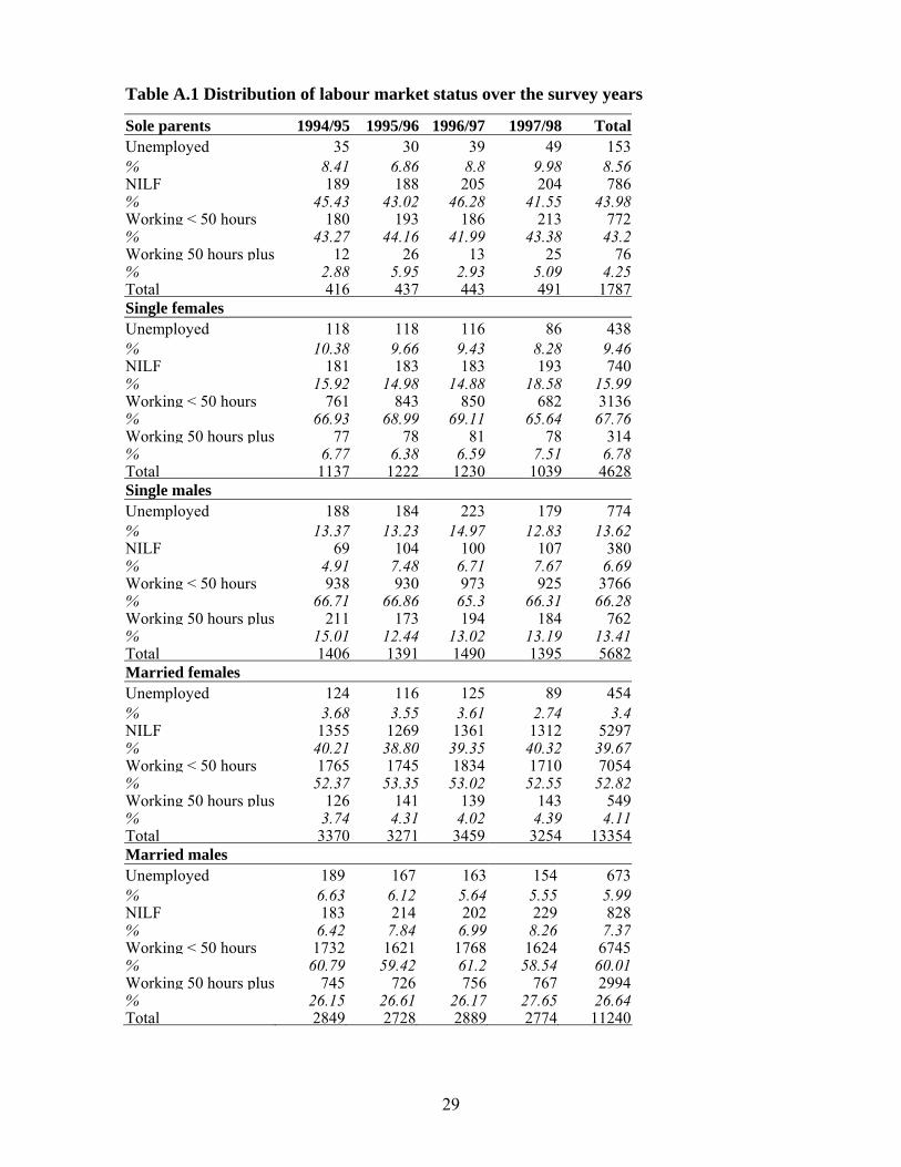
3 Table A.1 shows the proportion of people in the different demographic groups, who work 50 hours or more. Except for sole parents, a substantial number of people fall into this category. 4 In the four surveys used, there were 1035 people either at school or studying full-time. There were 18 unpaid voluntary workers and 283 individuals permanently unavailable for work. Also, there were 8141 individuals over the age of sixty-five. There were 4978 self-employed persons.

7

The four surveys were pooled5 and the sample was divided into five demographic groups.

These are: sole parents; single females without dependents; single males without

dependents; married females; and married males. Summary tables of sample characteristics

are provided for each demographic group in the Appendix. It was not possible to estimate

separate equations for sole mothers and sole fathers, given the small number of sole fathers

in the sample6.

Table 1 presents the average real wage rates across the four years for the five demographic

groups. Here it can be seen that, once average wage inflation has been accounted for,

average wages do not seem to change systematically between the various survey years. In

estimation, we include year dummies in the wage equation to check more formally for

systematic differences.

Table 1: Average real wage rates for 1994/95 to 1997/98, inflated to May 1998 level

1994/95 1995/96 1996/97 1997/98

Sole parents 14.79 15.56 16.51 15.66

Single females 14.08 13.76 14.04 14.42

Single males 14.64 14.69 15.03 15.10

Married females 15.96 16.00 15.82 15.95

Married males 18.70 18.76 19.02 18.94

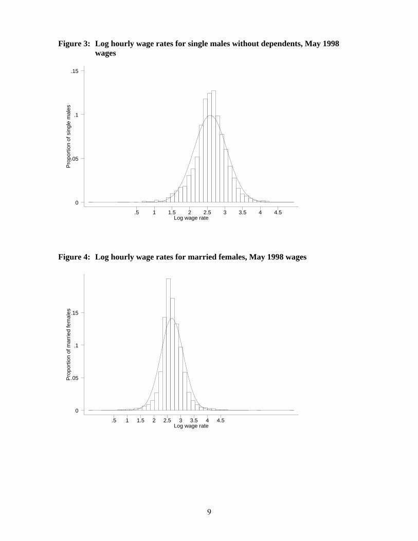
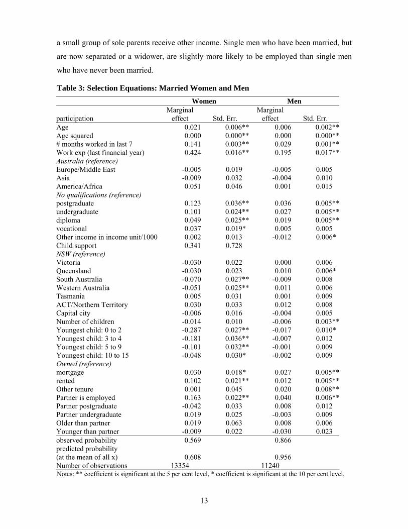
Examples of distributions of the logarithms of observed hourly wage rates for the five

demographic groups are shown in Figures 1 to 5. These are based on May 1998 wages and

the censoring of labour supply over 50 hours per week is not taken into account. The

histograms suggest that these distributions are approximately lognormal, although they are

slightly more peaked than the corresponding normal distributions with the same mean and

variance. Individuals reporting wage rates lower than $4 an hour or greater than $100 an

hour are considered outliers and are omitted from the wage equation. These observations

remain in the participation equation. As expected, the graphs show that the modal wage rate

is higher for men than for women.

5 All wage rates are uprated to 1998 using indices derived from average weekly earnings for males and females respectively and all income from other sources is inflated with the appropriate consumer price index to obtain the value it would have had in 1998. 6 There were 194 male sole parents, compared with 1593 females.

8

Figure 1: Log hourly wage rates for sole parents, May 1998 wages

Pr

opor

tion

of s

ole

pare

nts

Log wage rate.5 1 1.5 2 2.5 3 3.5 4 4.5

0

.05

.1

.15

Figure 2: Log hourly wage rates for single females without dependents, May 1998 wages

Pr

opor

tion

of s

ingl

e fe

mal

es

Log wage rate.5 1 1.5 2 2.5 3 3.5 4 4.5

0

.05

.1

.15

9

Figure 3: Log hourly wage rates for single males without dependents, May 1998 wages

P

ropo

rtion

of s

ingl

e m

ales

Log wage rate.5 1 1.5 2 2.5 3 3.5 4 4.5

0

.05

.1

.15

Figure 4: Log hourly wage rates for married females, May 1998 wages

P

ropo

rtion

of m

arrie

d fe

mal

es

Log wage rate.5 1 1.5 2 2.5 3 3.5 4 4.5

0

.05

.1

.15

10

Figure 5: Log hourly wage rates for married males, May 1998 wages

P

ropo

rtion

of m

arrie

d m

ales

Log wage rate.5 1 1.5 2 2.5 3 3.5 4 4.5

0

.05

.1

.15

4 Empirical Results This section presents the main empirical results. The selection equations, along with

specification tests and `hit and miss' tables, are reported in subsection 4.1. The wage

equations and associated specification tests are reported in subsection 4.2.

4.1 Selection Equations

The selection equations for each demographic group are based on sample sizes, for married

women, married men, single women, single men and sole parents of respectively 13354,

11240, 4628, 5682 and 1787 individuals. Tables 3, 4 and 5 present the marginal effects on

the probability of being employed, evaluated at sample means of variables and changing

the relevant variable by one unit (in most cases these marginal effects are the effects of a

discrete change from 0 to 1 in the dummy variable). The majority of coefficients are

significantly different from zero and the coefficients’ signs appear to accord with

expectations7.

7 Direct comparisons with results in Miller and Rummery (1991) are not possible because the latter distinguish only two demographic groups (males and females) and include a much smaller set of variables than is used here. The results from the participation equation in Creedy et al. (2001) cannot be directly compared because their sample does only include non-participants who are looking for work.

11

Before discussing the estimation results, a `hit and miss' table of actual versus predicted

values can be constructed to evaluate how well the selection model predicts (see Table 2).

The models generally tend to overpredict the empirically most frequently chosen outcome.

Indeed, this is true of the present models, with the employed being somewhat overpredicted

for each demographic group, except for sole parents where the non-working category is

largest. Such a result stems from the fact that the random elements of the model are

explicitly ignored in its evaluation.

Table 2: Predicted versus actual probabilities

Actual Predicted Not working Working TotalMarried women Not working 5151 527 5678Working 600 7076 7676Total 5751 7603 13354Married men Not working 1008 208 1216Working 493 9531 10024Total 1501 9739 11240Single females Not working 908 166 1074Working 270 3284 3554Total 1178 3450 4628Single males Not working 644 217 861Working 510 4311 4821Total 1154 4528 5682Sole parents Not working 863 120 983Working 76 728 804Total 939 848 1787

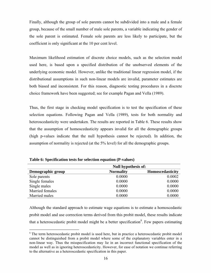
Considering the results in Tables 3 to 5, we find that age affects the probability of labour

force participation with the exception of sole parents, where the effect of age is

insignificant. Using the underlying coefficients for age and age squared, we find that age

has a positive effect on labour force participation for single women, married men and

women up to an age of around 30 years. After this age, a further increase in age means a

decrease in the probability of labour force participation. For single men, the maximum

probability seems to occur at a much younger age (around 20 years). Employment status is

unaffected by the number of children, apart from having a slight negative effect on the

12

probability of married men being in work. Although the number of dependent children has

no significant effect on the participation decision, the age of the youngest child is an

important factor in the participation probability of married women and sole parents, while

there is hardly an effect for married men. As expected, women with younger families

(particularly those with children under 5 years old) are less likely to participate. The effects

seem somewhat larger for sole parents than for married women. Sole parents receiving

child support are less likely to participate, whereas receipt of child support does not affect

the participation of married women significantly.

In the case of married women the probability of employment is higher for those with a

tertiary qualification than for those without any qualification, whereas a similar but smaller

effect is observed for married men. The size of the effects for singles without dependents is

in between those for married men and married women, with similar effects for males and

females. The probability of employment is higher for sole parents with a vocational

qualification than for those without any qualification, whereas the effects of the other

qualifications are of a similar size but insignificant. Surprisingly, the effect of a

postgraduate qualification was insignificant and small. The number of sole parents with a

postgraduate qualification is small, therefore we have included them in the reference group.

Previous work experience (as measured by the number of months in work of the last seven

months and whether there was any income from wages and salaries in the last financial

year) has a positive effect on participation probabilities. This effect is largest for married

women and sole parents and lowest for married men. The effect for singles is in between

these two effects with the effect for single men and women being similar in size.

Other income in the income unit (that is income for the income unit that is not derived from

benefits or from wages and salaries of the relevant individual) has a negative effect on the

participation of singles, which is largest for single women. There is hardly any effect on

participation for members of a couple. Individuals whose partner is employed are

significantly more likely to be in employment than couples where the partner is out of

work. This is particularly true for women. The other partner variables do not seem to have

much effect on the probability of employment. Other income seems to have a positive

effect on the participation probability of sole parents. However, it should be noted that only

13

a small group of sole parents receive other income. Single men who have been married, but

are now separated or a widower, are slightly more likely to be employed than single men

who have never been married.

Table 3: Selection Equations: Married Women and Men Women Men

participation Marginal

effect Std. Err. Marginal

effect Std. Err. Age 0.021 0.006** 0.006 0.002**Age squared 0.000 0.000** 0.000 0.000**# months worked in last 7 0.141 0.003** 0.029 0.001**Work exp (last financial year) 0.424 0.016** 0.195 0.017**Australia (reference) Europe/Middle East -0.005 0.019 -0.005 0.005 Asia -0.009 0.032 -0.004 0.010 America/Africa 0.051 0.046 0.001 0.015 No qualifications (reference) postgraduate 0.123 0.036** 0.036 0.005**undergraduate 0.101 0.024** 0.027 0.005**diploma 0.049 0.025** 0.019 0.005**vocational 0.037 0.019* 0.005 0.005 Other income in income unit/1000 0.002 0.013 -0.012 0.006*Child support 0.341 0.728 NSW (reference) Victoria -0.030 0.022 0.000 0.006 Queensland -0.030 0.023 0.010 0.006*South Australia -0.070 0.027** -0.009 0.008 Western Australia -0.051 0.025** 0.011 0.006 Tasmania 0.005 0.031 0.001 0.009 ACT/Northern Territory 0.030 0.033 0.012 0.008 Capital city -0.006 0.016 -0.004 0.005 Number of children -0.014 0.010 -0.006 0.003**Youngest child: 0 to 2 -0.287 0.027** -0.017 0.010*Youngest child: 3 to 4 -0.181 0.036** -0.007 0.012 Youngest child: 5 to 9 -0.101 0.032** -0.001 0.009 Youngest child: 10 to 15 -0.048 0.030* -0.002 0.009 Owned (reference) mortgage 0.030 0.018* 0.027 0.005**rented 0.102 0.021** 0.012 0.005**Other tenure 0.001 0.045 0.020 0.008**Partner is employed 0.163 0.022** 0.040 0.006**Partner postgraduate -0.042 0.033 0.008 0.012 Partner undergraduate 0.019 0.025 -0.003 0.009 Older than partner 0.019 0.063 0.008 0.006 Younger than partner -0.009 0.022 -0.030 0.023 observed probability 0.569 0.866 predicted probability (at the mean of all x) 0.608 0.956 Number of observations 13354 11240 Notes: ** coefficient is significant at the 5 per cent level, * coefficient is significant at the 10 per cent level.

14

Table 4: Selection Terms, Single Men and Women Single females Single males

participation Marginal

effect Std. Err.Marginal

effect Std. Err.Age 0.013 0.003** 0.003 0.002 Age squared 0.000 0.000** 0.000 0.000**# months worked in last 7 0.068 0.003** 0.053 0.002**Work exp (last financial year) 0.208 0.025** 0.218 0.020**Separated/widowed -0.012 0.024 0.028 0.014**Australia (reference) Europe/Middle East -0.051 0.025** -0.022 0.017 Asia 0.016 0.031 -0.069 0.034**Americas/Africa -0.045 0.058 0.015 0.036 No qualifications (reference) postgraduate 0.047 0.030 0.074 0.018**undergraduate 0.071 0.016** 0.091 0.010**diploma 0.050 0.019** 0.061 0.013**vocational -0.004 0.017 0.008 0.011 Other income in income unit/1000 -0.226 0.085** -0.138 0.067**NSW (reference) Victoria 0.008 0.019 -0.033 0.016**Queensland -0.005 0.020 -0.012 0.016 South Australia -0.074 0.029** -0.038 0.020**Western Australia 0.024 0.021 0.006 0.016 Tasmania -0.009 0.029 -0.054 0.026**ACT/Northern Territory 0.012 0.029 0.013 0.021 Capital city 0.023 0.015 0.008 0.011 Owned (reference) mortgage 0.086 0.019** 0.042 0.019**rented 0.011 0.024 0.032 0.020*Other tenure -0.095 0.034** -0.019 0.023 Observed probability 0.745 0.797 Predicted probability (at the mean of all x) 0.869 0.884 Number of observations 4628 5682 Notes: ** coefficient is significant at the 5 per cent level, * coefficient is significant at the 10 per cent level.

15

Table 5: Selection Terms: Sole Parents

participation Marginal effect Standard Errorfemale -0.125 0.061* Age 0.004 0.017 Age squared 0.000 0.000 # months worked in last 7 0.169 0.009** Work exp (last financial year) 0.302 0.039** Separated/widowed 0.071 0.048 Australia (reference) Europe/Middle East -0.086 0.059 Asia -0.234 0.082** America/Africa 0.073 0.123 No qualifications (reference) undergraduate 0.094 0.083 diploma 0.116 0.070 vocational 0.084 0.047* Other income in income unit/1000 0.415 0.341** Child support -0.656 0.321* NSW (reference) Victoria 0.080 0.058 Queensland 0.106 0.059* South Australia 0.048 0.068 Western Australia 0.133 0.064** Tasmania 0.158 0.074** ACT/Northern Territory 0.105 0.084 Capital city -0.014 0.041 Number of Children -0.032 0.025 Youngest child: 0 to 2 -0.315 0.082** Youngest child: 3 to 4 -0.219 0.086** Youngest child: 5 to 9 -0.121 0.079 Youngest child: 10 to 15 -0.109 0.072 Owned (reference) mortgage 0.040 0.072 rented 0.138 0.066** Other tenure 0.044 0.106 Observed probability 0.475 Predicted probability 0.501(at the mean of all x) Number of observations 1787 Notes: ** coefficient is significant at the 5 per cent level, * coefficient is significant at the 10 per cent level.

In addition to the variables relating to age, education, work experience and household

composition, it is found that all groups are more likely to be employed if their homes are

either rented or if they have a mortgage (as opposed to owning their home outright).

However this effect is not always significant. There is no clear pattern in the effect of the

state of residence on employment patterns, and living in a capital city is not significant for

any of the demographic groups.

16

Finally, although the group of sole parents cannot be subdivided into a male and a female

group, because of the small number of male sole parents, a variable indicating the gender of

the sole parent is estimated. Female sole parents are less likely to participate, but the

coefficient is only significant at the 10 per cent level.

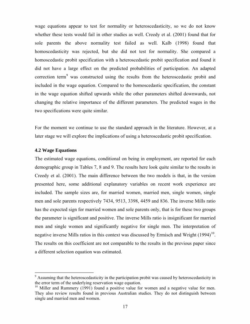
Maximum likelihood estimation of discrete choice models, such as the selection model

used here, is based upon a specified distribution of the unobserved elements of the

underlying economic model. However, unlike the traditional linear regression model, if the

distributional assumptions in such non-linear models are invalid, parameter estimates are

both biased and inconsistent. For this reason, diagnostic testing procedures in a discrete

choice framework have been suggested; see for example Pagan and Vella (1989).

Thus, the first stage in checking model specification is to test the specification of these

selection equations. Following Pagan and Vella (1989), tests for both normality and

heteroscedasticity were undertaken. The results are reported in Table 6. These results show

that the assumption of homoscedasticity appears invalid for all the demographic groups

(high p-values indicate that the null hypothesis cannot be rejected). In addition, the

assumption of normality is rejected (at the 5% level) for all the demographic groups.

Table 6: Specification tests for selection equation (P-values)

Null hypothesis of: Demographic group Normality HomoscedasticitySole parents 0.0000 0.0002Single females 0.0000 0.0000Single males 0.0000 0.0000Married females 0.0000 0.0000Married males 0.0000 0.0000

Although the standard approach to estimate wage equations is to estimate a homoscedastic

probit model and use correction terms derived from this probit model, these results indicate

that a heteroscedastic probit model might be a better specification8. Few papers estimating

8 The term heteroscedastic probit model is used here, but in practice a heteroscedastic probit model cannot be distinguished from a probit model where some of the explanatory variables enter in a non-linear way. Thus the misspecification may lie in an incorrect functional specification of the model as well as in ignoring heteroscedasticity. However, for ease of notation we continue referring to the alternative as a heteroscedastic specification in this paper.

17

wage equations appear to test for normality or heteroscedasticity, so we do not know

whether these tests would fail in other studies as well. Creedy et al. (2001) found that for

sole parents the above normality test failed as well. Kalb (1998) found that

homoscedasticity was rejected, but she did not test for normality. She compared a

homoscedastic probit specification with a heteroscedastic probit specification and found it

did not have a large effect on the predicted probabilities of participation. An adapted

correction term9 was constructed using the results from the heteroscedastic probit and

included in the wage equation. Compared to the homoscedastic specification, the constant

in the wage equation shifted upwards while the other parameters shifted downwards, not

changing the relative importance of the different parameters. The predicted wages in the

two specifications were quite similar.

For the moment we continue to use the standard approach in the literature. However, at a

later stage we will explore the implications of using a heteroscedastic probit specification.

4.2 Wage Equations

The estimated wage equations, conditional on being in employment, are reported for each

demographic group in Tables 7, 8 and 9. The results here look quite similar to the results in

Creedy et al. (2001). The main difference between the two models is that, in the version

presented here, some additional explanatory variables on recent work experience are

included. The sample sizes are, for married women, married men, single women, single

men and sole parents respectively 7434, 9513, 3398, 4459 and 836. The inverse Mills ratio

has the expected sign for married women and sole parents only, that is for these two groups

the parameter is significant and positive. The inverse Mills ratio is insignificant for married

men and single women and significantly negative for single men. The interpretation of

negative inverse Mills ratios in this context was discussed by Ermisch and Wright (1994)10.

The results on this coefficient are not comparable to the results in the previous paper since

a different selection equation was estimated.

9 Assuming that the heteroscedasticity in the participation probit was caused by heteroscedasticity in the error term of the underlying reservation wage equation. 10 Miller and Rummery (1991) found a positive value for women and a negative value for men. They also review results found in previous Australian studies. They do not distinguish between single and married men and women.

18

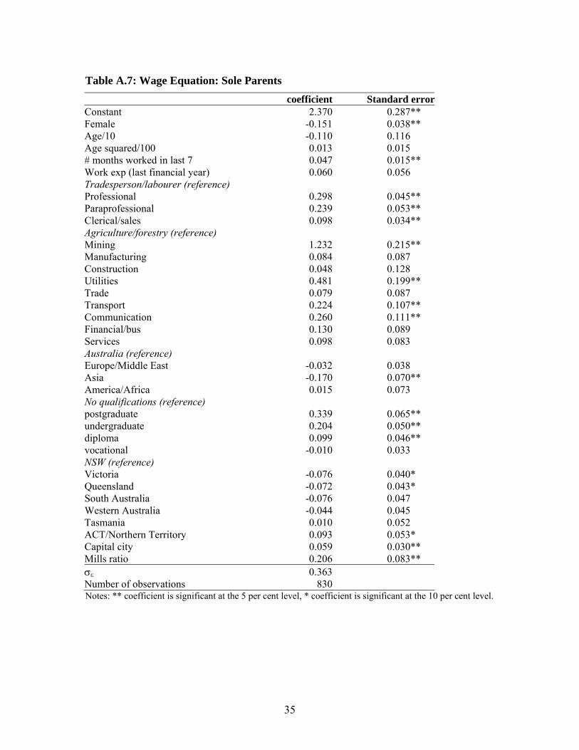
Here all models are presented with the Mills ratio included. However to impute wages for

non-workers, the equations for married men and singles are re-estimated using the interval

regression specification without the selection correction.

Table 7: Wage Equations: Married Women and Men Women Men coefficients s.e.'s coefficients s.e.'s constant 1.662 0.088** 1.755 0.086** Age/10 0.207 0.033** 0.206 0.031** Age squared/100 -0.025 0.004** -0.022 0.004** # months worked in last 7 0.020 0.005** 0.005 0.004 Work exp (last financial year) 0.169 0.028** 0.151 0.029** Tradesperson/labourer (reference) Professional 0.284 0.017** 0.125 0.011** Paraprofessional 0.216 0.018** 0.111 0.014** Clerical/sales 0.112 0.012** 0.056 0.012** Agriculture/forestry (reference) Mining 0.268 0.064** 0.613 0.034** Manufacturing 0.121 0.034** 0.281 0.025** Construction 0.267 0.045** 0.228 0.027** Utilities 0.259 0.070** 0.413 0.035** Trade 0.067 0.033** 0.129 0.025** Transport 0.188 0.043** 0.266 0.027** Communication 0.195 0.048** 0.355 0.032** Financial/bus 0.146 0.034** 0.264 0.026** Services 0.098 0.032** 0.240 0.025** Australia (reference) Europe/Middle East -0.014 0.012 -0.019 0.010* Asia -0.060 0.020** -0.102 0.018** America/Africa -0.037 0.027 -0.079 0.027** No qualifications (reference) postgraduate 0.128 0.054** 0.112 0.051** undergraduate 0.087 0.049* 0.052 0.048 diploma 0.092 0.015** 0.132 0.013** vocational 0.025 0.011** 0.057 0.010** NSW (reference) Victoria -0.039 0.013** -0.057 0.012** Queensland -0.061 0.013** -0.039 0.012** South Australia -0.052 0.015** -0.077 0.014** Western Australia -0.061 0.015** -0.034 0.013** Tasmania -0.045 0.019** -0.031 0.017* ACT/Northern Territory 0.068 0.018** 0.071 0.017** Capital city 0.054 0.010** 0.058 0.009** Age * university degree 0.021 0.012* 0.042 0.011** Mills ratio 0.127 0.031** 0.011 0.044 σε 0.356 0.373 Number of observations 7434 9513

Notes: ** coefficient is significant at the 5 per cent level, * coefficient is significant at the 10 per cent level.

19

Table 8: Wage Equations, Single Women and Men Women Men coefficients s.e.'s coefficients s.e.'sconstant 1.177 0.091** 1.012 0.087**Age/10 0.590 0.031** 0.657 0.030**Age squared/100 -0.068 0.004** -0.075 0.004**# months worked in last 7 -0.010 0.005** -0.014 0.005**Work exp (last financial year) 0.137 0.029** 0.101 0.031**Tradesperson/labourer (reference) Professional 0.185 0.021** 0.176 0.018**Paraprofessional 0.178 0.023** 0.123 0.021**Clerical/sales 0.084 0.016** 0.080 0.015**Agriculture/forestry (reference) Mining 0.497 0.115** 0.587 0.053**Manufacturing 0.039 0.053 0.237 0.029**Construction 0.065 0.069 0.253 0.031**Utilities 0.211 0.110* 0.436 0.052**Trade 0.016 0.052 0.130 0.029**Transport 0.205 0.059** 0.314 0.034**Communication 0.178 0.067** 0.343 0.041**Financial/bus 0.085 0.052 0.251 0.031**Services 0.060 0.051 0.210 0.029**Australia (reference) Europe/Middle East -0.008 0.018 0.005 0.018 Asia -0.031 0.027 -0.033 0.030 America/Africa -0.043 0.045 0.039 0.044 No qualifications (reference) postgraduate 0.114 0.049** 0.104 0.068 undergraduate 0.067 0.042 0.078 0.055 diploma 0.083 0.018** 0.066 0.020**vocational 0.069 0.014** 0.101 0.013**NSW (reference) Victoria -0.017 0.015 0.008 0.015 Queensland -0.050 0.016** -0.005 0.016 South Australia -0.001 0.019 -0.030 0.019 Western Australia -0.048 0.018** 0.008 0.017 Tasmania -0.017 0.023 -0.019 0.024 ACT/Northern Territory 0.091 0.025** 0.033 0.024 Capital city 0.040 0.012** 0.026 0.013**Age * university degree 0.027 0.012** 0.012 0.016 Mills ratio -0.068 0.044 -0.113 0.058**σε 0.292 0.342 Number of observations 3398 4459

Notes: ** coefficient is significant at the 5 per cent level, * coefficient is significant at the 10 per cent level.

20

Table 9: Wage Equation: Sole Parents coefficient Standard errorConstant 2.316 0.293** Female -0.132 0.039** Age/10 -0.101 0.119 Age squared/100 0.011 0.015 # months worked in last 7 0.048 0.015** Work exp (last financial year) 0.078 0.057 Tradesperson/labourer (reference) Professional 0.268 0.046** Paraprofessional 0.215 0.054** Clerical/sales 0.099 0.034** Agriculture/forestry (reference) Mining 1.034 0.219** Manufacturing 0.053 0.089 Construction 0.032 0.130 Utilities 0.444 0.203** Trade 0.055 0.089 Transport 0.228 0.109** Communication 0.238 0.113** Financial/bus 0.117 0.090 Services 0.093 0.085 Australia (reference) Europe/Middle East -0.019 0.039 Asia -0.139 0.072* America/Africa -0.004 0.075 No qualifications (reference) postgraduate 0.268 0.067** undergraduate 0.205 0.052** diploma 0.097 0.047** vocational -0.019 0.033 NSW (reference) Victoria -0.058 0.041 Queensland -0.045 0.044 South Australia -0.055 0.048 Western Australia -0.026 0.046 Tasmania 0.035 0.053 ACT/Northern Territory 0.108 0.054** Capital city 0.057 0.030* Mills ratio 0.220 0.084** σε 0.371 Number of observations 830 Notes: ** coefficient is significant at the 5 per cent level, * coefficient is significant at the 10 per cent level.

To ensure that the changes over time in the proportion of people in unemployment and out

of the labour force combined, and those in employment11 did not affect the estimated

11 See Table A.1 for the proportion of respondents in the different labour market states in each of the survey years.

21

results, a wage equation including year dummies for each of the survey years has been

estimated. These dummies turned out to be insignificant, indicating that after taking into

account the changes in average wage rates for men and women separately, wages do not

appear to differ significantly over the years.

The coefficients more or less display the expected variation of wage with age, that is wage

rates generally increase with age up to people’s early forties, after which they decline again

with age. The exception is the sole parents group, where no effect from age is found. The

age effect is more important for singles than for couples.

There is a considerable amount of difference in wage rates between occupations and

educational qualifications. Wage rates of professionals, paraprofessionals, and clerical or

salespersons are significantly higher than for trades persons or labourers across all groups.

As expected, the wage level is highest for professionals, followed by paraprofessionals and

then clerical or salespersons. Wage rates also tend to increase with the level of educational

qualification across all groups. Generally, people educated at university level have the

highest wages, although for single men a vocational education seems just as beneficial.

Sole parents with a diploma receive considerably lower wages compared to sole parents

with a postgraduate or undergraduate degree, followed by sole parents with a vocational

qualification. The significance of the interaction term between age and education level

(distinguishing between university level or less) indicates that the effects of age and

education are not completely independent of each other. For single women and married

couples the coefficient indicates that people with a university degree, have wages that

increase more with age than people without a university degree. This might indicate that

work experience results in more wage growth for people with a higher education level.

Work experience in the previous financial year has a positive effect on the current wage

level. However, the number of months in employment out of the last seven has little, and

sometimes even a negative, effect; only for married women and sole parents is the effect

positive and significant. The latter group, in particular, has a wage premium for recent work

experience, but on the other hand, the effect of work experience in the last financial year is

smaller than for other groups (and insignificant).

22

Couples living in NSW experience higher wage rates than those living in the other states,

with the exception of those residing in the Territories who receive even higher wages;

residents of the ACT form the larger part of this category. People living in capital cities are

paid higher wage rates than their counterparts living in other areas of the

country. Wage rates of married women and married or single men are higher in all

industries compared with the agriculture/forestry industry (the reference industry). For

single women and sole parents only the wage rates in mining, utilities, transport and

communication are significantly higher. People in the mining and utilities industries

generally have the highest wages, for men and sole parents the difference between these

and other industries is particularly high. The differences in wage rates between industries is

smallest for married women.

There seems to be little effect on wages depending on the country of origin. Only

immigrants from Asia earn significantly lower wages if they are in the groups of sole

parents or married men or women. Married men from America and Africa earn less than

those born in Australia. The effects for singles are insignificant and smaller in size. This

perhaps reflects a difference in the effect of being an immigrant between younger (who are

more likely to be single) and older age groups.

Female sole parents earn significantly less than male sole parents. Comparing the size of

the coefficient with the difference in the constant terms in the wage equations for married

men and women and in the equations for single men and women, it appears that the gender

difference in wages for sole parents is similar to the gender difference for the other groups.

Finally, the estimated standard error (σε) has a similar size over all the demographic

groups. It is largest for married men, indicating that for this group a larger proportion of the

differences in wage rates has not been explained by the variables included in the equation.

The standard error is smallest for single women, however, the differences between groups

are rather small.

The specification of the present model is based on the joint normality of both the selection

and regression equations. If the selection equation is misspecified, the same is true of the

correction term in the regression equation, resulting in biased and inconsistent estimates of

23

the determinants of wages; see Olsen (1982). Following Pagan and Vella (1989) it is

possible to test the assumption of joint normality by including the product of the linear

prediction terms of the selection equation (raised to powers 1, 2 and 3) and the inverse

Mills ratio for each individual. The null hypothesis of joint normality is rejected if these

three additional variables are jointly significant. The Wald tests for these restrictions are

reported in Table 10.

Table 10: Joint normality tests (P-values)

Demographic group Null hypothesis of joint normality

Married women 0.0000

Married men 0.8058

Single women 0.0362

Single men 0.0001

Sole parents 0.7978

Table 10 shows that the null hypothesis of joint normality is rejected for three out of the

five regressions. For married men and sole parents the assumption of joint normality cannot

be rejected suggesting some confidence in the validity of these results. On the other hand,

one might be wary of placing too much emphasis on the results of the determinants of the

wages of singles and married females. Similar to the tests reported in Table 6, few studies

on estimating wage equations report these tests, so we do not know whether these tests fail

in other studies as well. Looking at Figures 1 through 5, the assumption of normality for the

logarithm of the wage rates seems reasonable, so perhaps allowing for heteroscedasticity in

the selection equation will improve the results from the above tests as well. However, as

indicated before we continue use of the standard approach for the moment.

5 Wage Predictions This section considers the question of how a wage rate may be assigned to unemployed

individuals. In the simple case where the selection and wage equations contain a common

set of variables, consider first the conditional mean log-wage rate, for an individual with

given characteristics. For those who are employed, this is given by:

24

( ) λ̂σ̂ρ̂β̂xwE 2ε

'i1Ei i+== (10)

Imputed wage rates for those who are unemployed can be obtained using the expression:

( ) ( )( )γ̂z1γ̂zφ

σ̂ρ̂-β̂xwE 'i

'i2

ε'i0Ei i Φ−

== (11)

The use of the conditional mean log-wage is perhaps the most obvious choice for the

predicted wage. It is also possible, for example, to take a random draw, for each individual,

from the relevant conditional distribution. Indeed, in labour supply analyses there is no

necessity to be restricted to using observed wage rates for those employed in the sample

period: it would also be possible to take random draws from the relevant conditional

distributions.

In the present context, the expression in (11) cannot be used without modification because

some variables used in the estimation of the wage functions are not available for non-

workers. In addition to the wage rate, neither the occupation nor the industry of non-

workers is known. Although these variables could not be included in the selection

equations, they were included in the wage equations because of their demonstrated

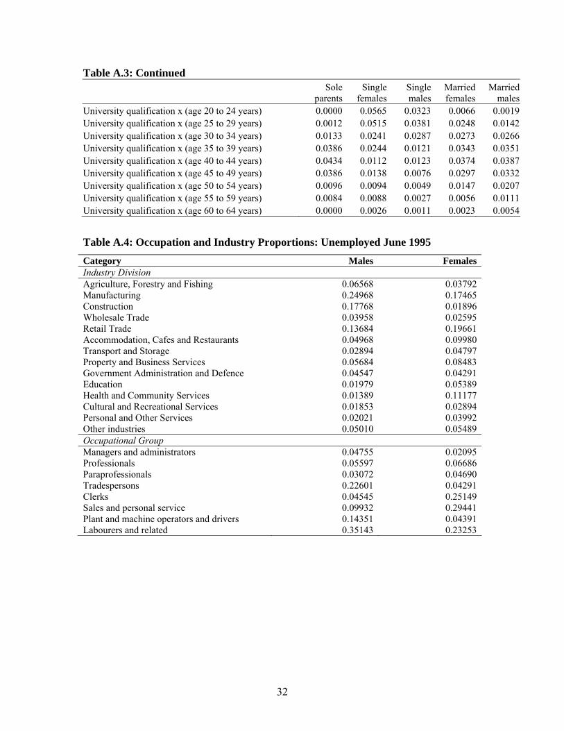
importance in wage determination. Extraneous information on unemployment rates within

the various occupation and industry groups are used to assign proportions within

occupation and industry groups to the non-workers (see Table A.4). For a complete

discussion of this see Creedy et al. (2001).

5.1 Marginal effects

This subsection provides selected examples of the extent to which a person’s wage rate

may change given a change in their observable characteristics.

Consider first what the impact of postgraduate qualifications is on the wage rates of

individuals. A typical sole parent or married female with a postgraduate degree is expected

to be offered a wage rate which is about 31 per cent higher than for those without post

25

secondary qualifications12. Single females without dependents and married men can expect

a return from postgraduate qualifications of about 12 per cent, while single males without

dependents exhibit the lowest (and insignificant) wage premium for a postgraduate

qualification with wage rates only 11 per cent higher.

Second, lets consider what impact living in a capital city has on the wage rate of

individuals. Wage rates are higher across all five demographic groups for individuals

residing in the capital city of their State. Single males experience the smallest effect on

their wage rates with less than a three per cent increase by living in a capital city. Sole

parents, single females and married males and females all have wage rates which are

between four and six per cent higher in capital cities.

Finally, consider what the impact of age is on the wage rates of individuals. To calculate

the age effect, we need to take into account the coefficients of age and age squared. In

addition the effect depends on the starting age. The effect for married men is an increase of

7.713 per cent for a ten-year increase in age from 25 to 35 years and a 3.0 per cent increase

for a ten-year increase from 35 to 45 years. This reflects the turnaround point in people’s

early forties, from an increasing wage rate with age to a decreasing wage rate with age.

5.2 Selected Examples of Predicted Wages

This subsection provides selected examples of predicted wages obtained when unemployed

individuals are assigned the sample occupation and industry characteristics.

Consider first a female unemployed sole parent with the following characteristics: aged 32

years; vocational qualification; no recent work experience; separated/widowed from a

previous relationship; European born; residing in ACT/NT in a non-capital city; with no

other income unit income; with two dependent children, one aged between 5 and 9 years

12 This value is calculated by using the following formula: [exp(relevant coefficient) – 1]×100%. In this example that is: [exp(0.268)-1] ×100% =30.7%. 13 The formula used in this calculation is [exp(coefficient of age + coefficient of age squared+2*(age at start/10)*(coefficient of age squared)) – 1]×100%. In this example that is: [exp(0.206-6*0.022)-1] ×100% =7.7%.

26

and the other between 10 and 15 years; living in ‘other tenure’. The predicted or imputed

wage obtained using (employed) sample averages for industry and occupation groups is

found to be $9.87 per hour. We can also calculate a predicted wage using the model, which

does not account for the censored labour supply observation14. This is $10.17, which is

only slightly higher than the specification accounting for the censoring of labour supply

over 49 hours. There are relatively few sole parents working long hours, so one would not

expect a large difference in the outcomes from the two specifications.

Second, consider a single female without children; never married; aged 22 years; Australian

born; residing outside the Sydney metropolitan region in NSW; with a vocational

qualification; no recent work experience; living in ‘other tenure’ with no other

income. The imputed hourly wage is found to be $10.48 ($10.63 in the model which does

not account for censoring in labour supply).

Third, consider an unemployed single male without children; never married; aged 22 years;

vocational qualification; no recent work experience; Australian born residing outside the

Brisbane metropolitan region in Queensland; in rented accommodation. The imputed wage

is $11.06 ($11.56 in the model which does not account for censoring in labour supply).

Fourth, consider an unemployed married female: aged 42 years; with one dependent child

aged over 15 years; European born; residing in Perth; without formal educational

qualifications; no recent work experience, but worked during last financial year; partner has

vocational qualification but is currently not employed; other income is $25 per week; owns

home outright. The basic imputed wage is $12.32 per hour ($12.70 in the model which does

not account for censoring in labour supply).

Finally, consider an unemployed married male: aged 47 years with five dependent children

(three of which are aged 5 to 9 years, two are aged 10 to 15 years); European born; residing

in Melbourne; with a diploma; no recent work experience, but worked during last financial

14 The coefficients for the models not accounting for the censoring of labour supply at 50 hours can be found in Tables A.5 to A7.

27

year; partner has no formal qualifications and is currently not employed; no other income;

owns home outright. The basic hourly rate is $21.44 per hour. In a model not taking into

account the censoring of labour supply over 49 hours per week this would have been

$25.22. The difference for married men between the two specifications is much larger than

for the other groups, because a large proportion of the group of married men falls in the

category, which works 50 hours or more. Thus accounting for censoring of labour supply is

more important in this group.

6 Conclusion This paper has reported estimates of wage equations for Australian workers, using pooled

data from the Income and Housing Costs Surveys for 1994/95, 1995/96, 1996/97 and

1997/98, the first four years for which continuous hours information is available for each

individual. The process of assigning a wage rate to non-workers, as necessary in the context

of labour supply analysis, was examined with special attention given to dealing with the

situation where the wage equation includes variables that are not available for the

unemployed (such as occupation and industry).

Additionally, wage information on individuals, who work more than 50 hours per week and

for whom the exact number of hours is therefore unknown in the SIHC, is included as a

range rather than approximated by an “exact” value. This prevents the overestimation of

wage rates.

Finally, normality and homoscedasticity of the participation equation and joint normality of

the participation and wage equation are tested in this paper. It was found that normality and

homoscedasticity of the participation equation is rejected for all groups and joint normality

is rejected for all groups except married men and sole parents. Given that most studies on

the estimation of wage equations do not carry out these tests, it is difficult to compare these

results to results from other studies. For the moment, we have continued to use the standard

approach to estimate the wage equations for the different demographic groups, but in future

research we will explore the implication of accounting for heteroscedasticity.

28

Appendix: Summary Statistics Summary statistics for the various demographic groups are shown in Tables A.2 and A.3.

Many variables are dummy variables taking (0,1) values, the tables show the proportions in

each category for these variables. The samples used in the selection equations and the wage

equations are different, so the summary statistics for each are reported in a separate table.

Information about the last full-time job of those unemployed in June 1995, taken from the

Labour Force Survey (ABS Catalogue, number 6203, Table 28), were used to construct the

proportions given in Table A.4.

29

Table A.1 Distribution of labour market status over the survey years

Sole parents 1994/95 1995/96 1996/97 1997/98 TotalUnemployed 35 30 39 49 153% 8.41 6.86 8.8 9.98 8.56NILF 189 188 205 204 786% 45.43 43.02 46.28 41.55 43.98Working < 50 hours 180 193 186 213 772% 43.27 44.16 41.99 43.38 43.2Working 50 hours plus 12 26 13 25 76% 2.88 5.95 2.93 5.09 4.25Total 416 437 443 491 1787Single females Unemployed 118 118 116 86 438% 10.38 9.66 9.43 8.28 9.46NILF 181 183 183 193 740% 15.92 14.98 14.88 18.58 15.99Working < 50 hours 761 843 850 682 3136% 66.93 68.99 69.11 65.64 67.76Working 50 hours plus 77 78 81 78 314% 6.77 6.38 6.59 7.51 6.78Total 1137 1222 1230 1039 4628Single males Unemployed 188 184 223 179 774% 13.37 13.23 14.97 12.83 13.62NILF 69 104 100 107 380% 4.91 7.48 6.71 7.67 6.69Working < 50 hours 938 930 973 925 3766% 66.71 66.86 65.3 66.31 66.28Working 50 hours plus 211 173 194 184 762% 15.01 12.44 13.02 13.19 13.41Total 1406 1391 1490 1395 5682Married females Unemployed 124 116 125 89 454% 3.68 3.55 3.61 2.74 3.4NILF 1355 1269 1361 1312 5297% 40.21 38.80 39.35 40.32 39.67Working < 50 hours 1765 1745 1834 1710 7054% 52.37 53.35 53.02 52.55 52.82Working 50 hours plus 126 141 139 143 549% 3.74 4.31 4.02 4.39 4.11Total 3370 3271 3459 3254 13354Married males Unemployed 189 167 163 154 673% 6.63 6.12 5.64 5.55 5.99NILF 183 214 202 229 828% 6.42 7.84 6.99 8.26 7.37Working < 50 hours 1732 1621 1768 1624 6745% 60.79 59.42 61.2 58.54 60.01Working 50 hours plus 745 726 756 767 2994% 26.15 26.61 26.17 27.65 26.64Total 2849 2728 2889 2774 11240

Table A.2: Sample Proportions: Selection Equations variable

Sole

parentsSingle

femalesSingle males

Married females

Married males

Age 15 to 19 years 0.0235 0.1469 0.1420 0.0055 0.0015Age 20 to 24 years 0.0755 0.2398 0.2763 0.0499 0.0334Age 25 to 29 years 0.1489 0.1497 0.1809 0.1149 0.0954Age 30 to 34 years 0.1796 0.0761 0.1156 0.1463 0.1452Age 35 to 39 years 0.2104 0.0575 0.0743 0.1538 0.1557Age 40 to 44 years 0.1919 0.0490 0.0669 0.1481 0.1531Age 45 to 49 years 0.1052 0.0674 0.0498 0.1354 0.1528Age 50 to 54 years 0.0386 0.0637 0.0357 0.1026 0.1150Age 55 to 59 years 0.0196 0.0646 0.0322 0.0747 0.0858Age 60 to 64 years 0.0067 0.0851 0.0262 0.0687 0.0622Number of months worked in last 7 2.8153 4.1940 4.3784 3.6451 5.3951Work experience (last financial year) 0.5462 0.7770 0.8416 0.6239 0.8917Separated/widowed 0.6961 0.2917 0.1681 Australia (reference) 0.8131 0.8332 0.8458 0.7313 0.7216Europe/Middle East 0.1226 0.1108 0.1058 0.1901 0.2069Asia 0.0425 0.0411 0.0341 0.0576 0.0510America/Africa 0.0218 0.0149 0.0143 0.0210 0.0206Postgraduate 0.0308 0.0428 0.0280 0.0392 0.0657Undergraduate 0.0616 0.1225 0.0949 0.0921 0.1077Diploma 0.0755 0.0914 0.0790 0.0878 0.1142Vocational qualification 0.1858 0.1709 0.2330 0.1714 0.2849No post secondary qualification (reference) 0.6463 0.5724 0.5651 0.6096 0.4274Other income/1000 0.0168 0.0157 0.0126 0.5794 0.3172Child support income/1000 0.0268 0.0008 0.0000NSW (reference) 0.2009 0.2349 0.2318 0.2262 0.2260Victoria 0.2059 0.2275 0.2082 0.2154 0.2150Queensland 0.1746 0.1793 0.1760 0.1747 0.1735South Australia 0.1276 0.1124 0.1153 0.1126 0.1077Western Australia 0.1393 0.1242 0.1369 0.1324 0.1335Tasmania 0.0783 0.0637 0.0598 0.0704 0.0717ACT/Northern Territory 0.0733 0.0579 0.0720 0.0682 0.0726Capital city 0.5993 0.6737 0.6341 0.6030 0.6113Number of dependents 1.7101 1.1116 1.1882Youngest child aged 0 to 2 years 0.1975 0.1672 0.1821Youngest child aged 3 to 4 years 0.1371 0.0673 0.0712Youngest child aged 5 to 9 years 0.2781 0.1290 0.1419Youngest child aged 10 to 15 years 0.2451 0.1180 0.1223Own home (reference) 0.1293 0.1547 0.0783 0.3679 0.3279Mortgage 0.2160 0.1214 0.1156 0.4152 0.4449Rented 0.6150 0.4983 0.5734 0.1915 0.2007Other tenure 0.0392 0.2234 0.2297 0.0238 0.0243Partner employed 0.7964 0.6117Partner has postgraduate qualification 0.0576 0.0405Partner has undergraduate qualification 0.0978 0.0987"Older" than partner 0.0108 0.1054"Younger" than partner 0.1321 0.0140

31

Table A.3: Sample Proportions: Wage Equations

Sole

parentsSingle

femalesSingle males

Married females

Married males

Age 15 to 19 years 0.0060 0.1345 0.1285 0.0044 0.0011Age 20 to 24 years 0.0325 0.2825 0.2830 0.0562 0.0324Age 25 to 29 years 0.1036 0.1810 0.1976 0.1236 0.1017Age 30 to 34 years 0.1602 0.0898 0.1247 0.1453 0.1528Age 35 to 39 years 0.2313 0.0683 0.0765 0.1668 0.1657Age 40 to 44 years 0.2410 0.0530 0.0684 0.1803 0.1624Age 45 to 49 years 0.1470 0.0730 0.0493 0.1659 0.1599Age 50 to 54 years 0.0530 0.0630 0.0325 0.1030 0.1164Age 55 to 59 years 0.0193 0.0415 0.0265 0.0421 0.0732Age 60 to 64 years 0.0060 0.0135 0.0130 0.0124 0.0346Number of months worked in last 7 5.4663 5.3799 5.1794 5.9295 6.0369Work experience (last financial year) 0.9048 0.9429 0.9343 0.9496 0.9687Professional 0.2253 0.2157 0.1801 0.2273 0.3107Paraprofessional 0.0819 0.0848 0.0760 0.0889 0.1052Clerical or sales person 0.4386 0.5630 0.1983 0.5163 0.1503Tradesperson or labourer 0.2542 0.1366 0.5456 0.1675 0.4337Agriculture/Forestry 0.0205 0.0088 0.0375 0.0145 0.0272Mining 0.0036 0.0024 0.0121 0.0054 0.0231Manufacturing 0.1084 0.0848 0.2023 0.0920 0.2054Construction 0.0157 0.0112 0.0931 0.0174 0.0803Utility 0.0048 0.0026 0.0126 0.0043 0.0209Retail/Wholesale Sales 0.1494 0.1995 0.2133 0.1672 0.1626Transport 0.0325 0.0297 0.0574 0.0203 0.0685Communications 0.0253 0.0135 0.0269 0.0132 0.0302Financial/Business Services 0.1169 0.1816 0.1216 0.1501 0.1317Other Services 0.5205 0.4647 0.2220 0.5133 0.2484Australian born 0.8060 0.8626 0.8531 0.7620 0.7333Europe/Middle East 0.1277 0.0862 0.1007 0.1660 0.1972Asia 0.0349 0.0386 0.0323 0.0479 0.0488America/Africa 0.0313 0.0127 0.0139 0.0241 0.0207Postgraduate 0.0554 0.0539 0.0327 0.0578 0.0713Undergraduate 0.0976 0.1486 0.1074 0.1248 0.1156Diploma 0.1024 0.1030 0.0848 0.1063 0.1178Vocational qualification 0.2145 0.1801 0.2436 0.1874 0.2913No post secondary qualifications 0.5301 0.5144 0.5315 0.5237 0.4040NSW (reference) 0.1831 0.2375 0.2368 0.2261 0.2247Victoria 0.2120 0.2360 0.2090 0.2127 0.2151Queensland 0.1639 0.1760 0.1736 0.1706 0.1737South Australia 0.1133 0.1015 0.1088 0.1134 0.1058Western Australia 0.1410 0.1263 0.1390 0.1263 0.1363Tasmania 0.0867 0.0606 0.0567 0.0647 0.0689ACT/Northern Territory 0.1000 0.0621 0.0760 0.0862 0.0756Capital city 0.6012 0.6933 0.6445 0.6166 0.6192

32

Table A.3: Continued

Sole

parentsSingle

femalesSingle males

Married females

Married males

University qualification x (age 20 to 24 years) 0.0000 0.0565 0.0323 0.0066 0.0019University qualification x (age 25 to 29 years) 0.0012 0.0515 0.0381 0.0248 0.0142University qualification x (age 30 to 34 years) 0.0133 0.0241 0.0287 0.0273 0.0266University qualification x (age 35 to 39 years) 0.0386 0.0244 0.0121 0.0343 0.0351University qualification x (age 40 to 44 years) 0.0434 0.0112 0.0123 0.0374 0.0387University qualification x (age 45 to 49 years) 0.0386 0.0138 0.0076 0.0297 0.0332University qualification x (age 50 to 54 years) 0.0096 0.0094 0.0049 0.0147 0.0207University qualification x (age 55 to 59 years) 0.0084 0.0088 0.0027 0.0056 0.0111University qualification x (age 60 to 64 years) 0.0000 0.0026 0.0011 0.0023 0.0054

Table A.4: Occupation and Industry Proportions: Unemployed June 1995

Category Males Females Industry Division Agriculture, Forestry and Fishing 0.06568 0.03792 Manufacturing 0.24968 0.17465 Construction 0.17768 0.01896 Wholesale Trade 0.03958 0.02595 Retail Trade 0.13684 0.19661 Accommodation, Cafes and Restaurants 0.04968 0.09980 Transport and Storage 0.02894 0.04797 Property and Business Services 0.05684 0.08483 Government Administration and Defence 0.04547 0.04291 Education 0.01979 0.05389 Health and Community Services 0.01389 0.11177 Cultural and Recreational Services 0.01853 0.02894 Personal and Other Services 0.02021 0.03992 Other industries 0.05010 0.05489 Occupational Group Managers and administrators 0.04755 0.02095 Professionals 0.05597 0.06686 Paraprofessionals 0.03072 0.04690 Tradespersons 0.22601 0.04291 Clerks 0.04545 0.25149 Sales and personal service 0.09932 0.29441 Plant and machine operators and drivers 0.14351 0.04391 Labourers and related 0.35143 0.23253

33

Table A.5: Wage Equations: Married Women and Men Women Men coefficients s.e.'s coefficients s.e.'s constant 1.717 0.086** 1.710 0.084** Age/10 0.201 0.032** 0.273 0.031** Age squared/100 -0.024 0.004** -0.031 0.004** # months worked in last 7 0.017 0.005** 0.003 0.004 Work exp (last financial year) 0.158 0.027** 0.159 0.028** Tradesperson/labourer (reference) Professional 0.317 0.016** 0.204 0.011** Paraprofessional 0.231 0.018** 0.157 0.014** Clerical/sales 0.112 0.012** 0.061 0.012** Agriculture/forestry (reference) Mining 0.260 0.062** 0.618 0.033** Manufacturing 0.112 0.033** 0.257 0.024** Construction 0.257 0.043** 0.231 0.026** Utilities 0.248 0.068** 0.337 0.035** Trade 0.060 0.033* 0.119 0.025** Transport 0.183 0.042** 0.292 0.027** Communication 0.183 0.047** 0.295 0.032** Financial/bus 0.139 0.033** 0.243 0.025** Services 0.082 0.031** 0.179 0.024** Australia (reference) Europe/Middle East -0.017 0.011 -0.031 0.010** Asia -0.062 0.019** -0.152 0.018** America/Africa -0.032 0.026 -0.093 0.027** No qualifications (reference) postgraduate 0.151 0.052** 0.079 0.050 undergraduate 0.097 0.048** -0.012 0.047 diploma 0.092 0.015** 0.136 0.013** vocational 0.024 0.011** 0.063 0.009** NSW (reference) Victoria -0.040 0.012** -0.055 0.011** Queensland -0.063 0.013** -0.044 0.012** South Australia -0.052 0.015** -0.086 0.014** Western Australia -0.062 0.014** -0.029 0.013** Tasmania -0.048 0.018** -0.049 0.017** ACT/Northern Territory 0.067 0.017** 0.070 0.017** Capital city 0.056 0.009** 0.066 0.009** Age * university degree 0.019 0.012* 0.056 0.011** Mills ratio 0.107 0.031** -0.005 0.043 σε 0.345 0.365 Number of observations 7434 9513

Notes: ** coefficient is significant at the 5 per cent level, * coefficient is significant at the 10 per cent level.

34

Table A.6: Wage Equations, Single Women and Men Women Men coefficients s.e.'s coefficients s.e.'sconstant 1.179 0.089** 1.021 0.087** Age/10 0.620 0.030** 0.696 0.030** Age squared/100 -0.072 0.004** -0.080 0.004** # months worked in last 7 -0.010 0.004** -0.016 0.005** Work exp (last financial year) 0.140 0.028** 0.101 0.031** Tradesperson/labourer (reference) Professional 0.217 0.020** 0.218 0.018** Paraprofessional 0.196 0.023** 0.136 0.021** Clerical/sales 0.084 0.016** 0.079 0.014** Agriculture/forestry (reference) Mining 0.545 0.112** 0.641 0.053** Manufacturing -0.001 0.052 0.205 0.029** Construction 0.058 0.068 0.235 0.031** Utilities 0.148 0.107 0.376 0.052** Trade -0.019 0.051 0.096 0.029** Transport 0.157 0.057** 0.304 0.034** Communication 0.139 0.065** 0.290 0.041** Financial/bus 0.051 0.051 0.223 0.031** Services 0.017 0.050 0.161 0.029** Australia (reference) Europe/Middle East -0.007 0.018 -0.001 0.018 Asia -0.047 0.026* -0.061 0.030** America/Africa -0.047 0.044 0.041 0.044 No qualifications (reference) postgraduate 0.109 0.048** 0.084 0.068 undergraduate 0.065 0.041 0.033 0.055 diploma 0.085 0.017** 0.080 0.020** vocational 0.069 0.014** 0.105 0.013** NSW (reference) Victoria -0.023 0.014 0.005 0.015 Queensland -0.048 0.016** -0.008 0.016 South Australia -0.003 0.019 -0.032 0.019* Western Australia -0.051 0.017** 0.021 0.017 Tasmania -0.024 0.023 -0.029 0.024 ACT/Northern Territory 0.086 0.024** 0.031 0.023 Capital city 0.041 0.012** 0.029 0.013** Age * university degree 0.031 0.011** 0.027 0.016* Mills ratio -0.068 0.043 -0.116 0.057** σε 0.284 0.341 Number of observations 3398 4459

Notes: ** coefficient is significant at the 5 per cent level, * coefficient is significant at the 10 per cent level.

35

Table A.7: Wage Equation: Sole Parents coefficient Standard errorConstant 2.370 0.287** Female -0.151 0.038** Age/10 -0.110 0.116 Age squared/100 0.013 0.015 # months worked in last 7 0.047 0.015** Work exp (last financial year) 0.060 0.056 Tradesperson/labourer (reference) Professional 0.298 0.045** Paraprofessional 0.239 0.053** Clerical/sales 0.098 0.034** Agriculture/forestry (reference) Mining 1.232 0.215** Manufacturing 0.084 0.087 Construction 0.048 0.128 Utilities 0.481 0.199** Trade 0.079 0.087 Transport 0.224 0.107** Communication 0.260 0.111** Financial/bus 0.130 0.089 Services 0.098 0.083 Australia (reference) Europe/Middle East -0.032 0.038 Asia -0.170 0.070** America/Africa 0.015 0.073 No qualifications (reference) postgraduate 0.339 0.065** undergraduate 0.204 0.050** diploma 0.099 0.046** vocational -0.010 0.033 NSW (reference) Victoria -0.076 0.040* Queensland -0.072 0.043* South Australia -0.076 0.047 Western Australia -0.044 0.045 Tasmania 0.010 0.052 ACT/Northern Territory 0.093 0.053* Capital city 0.059 0.030** Mills ratio 0.206 0.083** σε 0.363 Number of observations 830 Notes: ** coefficient is significant at the 5 per cent level, * coefficient is significant at the 10 per cent level.

36

References

Creedy, J., A. Duncan, M. Harris and R. Scutella (2001), “Wage functions: Australian

estimates using the Income Distribution Survey”, Australian Journal of Labour

Economics, 4(4), 300-321.

Ermisch, J. F. and Wright, R. E. (1994) Interpretation of negative sample selection effects

in wage offer equations. Applied Economics Letters, 1, pp. 187-189.

Greene, W. (1981) Sample selection bias as a specification error: comment.

Econometrica, 49, pp. 795-798.

Heckman, J. (1979) Sample selection bias as a specification error. Econometrica, 47, pp.

153-161.

Kalb, G. (1998) An Australian model for labour supply and welfare participation in two-

adult households. Unpublished thesis, Department of Econometrics and Business

Statistics, Monash University.

Maddala, G. S. (1983) Limited Dependent And Qualitative Variables in Econometrics.

Cambridge: Cambridge University Press.

Miller, P. and Rummery, S. (1991) Male-female wage differentials in Australia: a

reassessment. Australian Economic Papers, 30, pp. 50-69.

Olsen, R. (1982) Distributional tests for selectivity bias and a more robust estimator.

International Economic Review, 23, pp. 223-240.

Pagan, A. and Vella, F. (1989) Diagnostic tests for models based on individual data: a

survey. Journal of Applied Econometrics, 4, pp. s29- s59.