Estimation of Production Functionsaguirregabiria.net/.../book_dynamic_io_chapter_03.pdf52 3....
22
CHAPTER 3 Estimation of Production Functions 1. Introduction The estimation of rmscost functions in Empirical IO plays an important role in any empirical study of industry competition. As explained in chapter 1, data on production costs at the level of individual rm-market-product is very rare, and for this reason costs functions are typically estimated in an indirect way, using rst order conditions of optimality for prot maximization. However, a type of data that is more commonly available is cross- sectional or panel data with rm level information on output and inputs that the rm uses in the production process, such as labor, capital equipment, energy, materials, and other intermediate inputs. Given this information, it is possible to estimate a Production Function and use it to obtain rmscost functions. More generally, Production functions (PF) are important primitive components of many economic models. The estimation of PFs plays a key role in the empirical analysis of issues such as the contribution of di/erent factors to economic growth, the degree of complementarity and substitutability between inputs, skill-biased technological change, estimation of economies of scale and economies of scope, evaluation of the e/ects of new technologies, learning-by-doing, or the quantication of production externalities, among many others. There are multiple issues that should be taken into account in the estimation of pro- ductions functions. (a) Data problems: measurement error in output (typically we observe revenue but not output, and we do not have prices at the rm level); measurement error in capital (we observe the book value of capital, but not the economic value of capital); di/er- ences in the quality of labor; etc. (b) Specication problems: Functional form assumptions, particularly when we have di/erent types of labor and capital inputs such that there may be both complementarity and substitutability. (c) Simultaneity: Observed inputs (e.g., labor, capital) may be correlated with unobserved inputs or productivity shocks (e.g., managerial ability, quality of land, materials, capacity utilization). This correlation introduces biases in some estimators of PF parameters. (d) Multicollinearity: Typically, labor and capital inputs are highly correlated with each other. This collinearity may be an important problem for the precise estimation of PF parameters. (e) Endogenous Exit/Selection: In panel datasets, rmexit from the sample is not exogenous and it is correlated with rm size. Smaller rms 51
Transcript of Estimation of Production Functionsaguirregabiria.net/.../book_dynamic_io_chapter_03.pdf52 3....
CHAPTER 3
Estimation of Production Functions
1. Introduction
The estimation of �rms�cost functions in Empirical IO plays an important role in any
empirical study of industry competition. As explained in chapter 1, data on production
costs at the level of individual �rm-market-product is very rare, and for this reason costs
functions are typically estimated in an indirect way, using �rst order conditions of optimality
for pro�t maximization. However, a type of data that is more commonly available is cross-
sectional or panel data with �rm level information on output and inputs that the �rm
uses in the production process, such as labor, capital equipment, energy, materials, and
other intermediate inputs. Given this information, it is possible to estimate a Production
Function and use it to obtain �rms�cost functions. More generally, Production functions
(PF) are important primitive components of many economic models. The estimation of
PFs plays a key role in the empirical analysis of issues such as the contribution of di¤erent
factors to economic growth, the degree of complementarity and substitutability between
inputs, skill-biased technological change, estimation of economies of scale and economies of
scope, evaluation of the e¤ects of new technologies, learning-by-doing, or the quanti�cation
of production externalities, among many others.
There are multiple issues that should be taken into account in the estimation of pro-
ductions functions. (a) Data problems: measurement error in output (typically we observe
revenue but not output, and we do not have prices at the �rm level); measurement error in
capital (we observe the book value of capital, but not the economic value of capital); di¤er-
ences in the quality of labor; etc. (b) Speci�cation problems: Functional form assumptions,
particularly when we have di¤erent types of labor and capital inputs such that there may be
both complementarity and substitutability. (c) Simultaneity: Observed inputs (e.g., labor,
capital) may be correlated with unobserved inputs or productivity shocks (e.g., managerial
ability, quality of land, materials, capacity utilization). This correlation introduces biases in
some estimators of PF parameters. (d) Multicollinearity: Typically, labor and capital inputs
are highly correlated with each other. This collinearity may be an important problem for
the precise estimation of PF parameters. (e) Endogenous Exit/Selection: In panel datasets,
�rm exit from the sample is not exogenous and it is correlated with �rm size. Smaller �rms
51

52 3. ESTIMATION OF PRODUCTION FUNCTIONS
are more likely to exit than larger �rms. Endogenous exit introduces selection-biases in some
estimators of PF parameters.
In this chapter, we concentrate on the problems of simultaneity, multicollinearity, and
endogenous exit, and on di¤erent solutions that have been proposed to deal with these
issues. For the sake of simplicity, we discuss these issues in the context of a Cobb-Douglas
PF. However, the arguments and results can be extended to more general speci�cations
of PFs. In principle, some of the estimation approaches can be generalized to estimate
nonparametric speci�cations of PF. Griliches and Mairesse (1998), Bond and Van Reenen
(2007), and Ackerberg et al. (2007) include surveys of this literature. However, this is a very
active literature where there have substantial developments over the last �ve years.
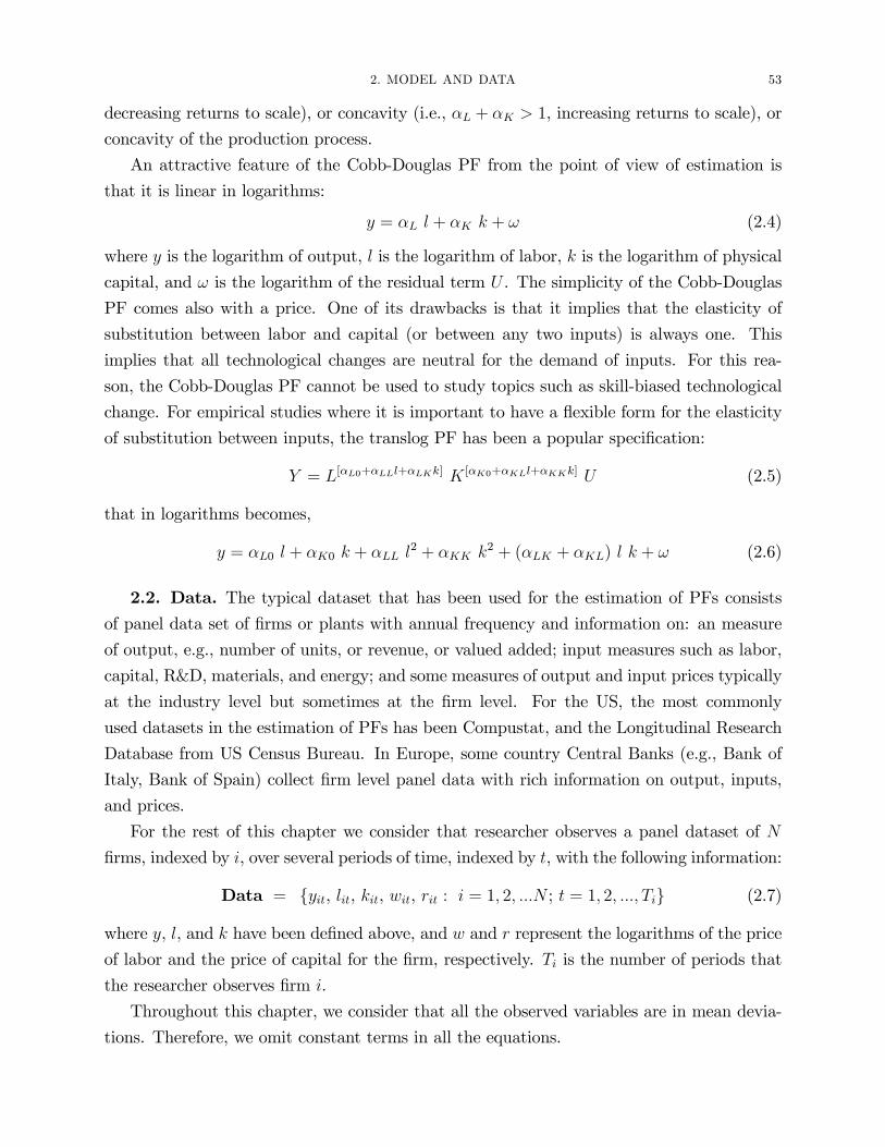
2. Model and Data
2.1. Model. A Production Function (PF) is a description of a production technologythat relates the physical output of a production process to the physical inputs or factors of
production. A general representation is:
Y = F (X1, X2, :::, XK , A) (2.1)
where Y is a measure of �rm output, X1, X2, ::, and XJ are measures of J �rm inputs, and
A represents the �rm technological e¢ ciency.
A very common speci�cation is the Cobb-Douglas PF (Cobb and Douglas, 1928, Ameri-
can Economic Review):
Y = L�L K�K U (2.2)
where L represents the labor input, K is capital, U represents the contribution to output of
technological e¢ ciency but also of any other input that is not labor or capital (e.g., materials,
energy), and �L and �K are technological (structural) parameters that are assumed the same
for all the �rms in the market and industry under study. This standard Cobb-Douglas PF
can be generalized to include explicitly more inputs, e.g., Y = L�L K�K R�R E�E U , where
R represents R&D and E is energy inputs. We can also distinguish di¤eerent types of labor
(blue collar and white collar labor), and capital (equipment, information technology).
Given the Cobb-Douglas PF, and input pricesW for labor and R for capital, the problem
of cost minimization for the �rm implies the following Cost Function:
C(Y ) = W�L
�L+�K R�K
�L+�K Q1
�L+�K (2.3)
where is a positive constant that depends (only) on the parameters �L and �K . This
expression shows that the parameter �L+�K determines the economies of scale in production
and the linearity (i.e., �L+�K = 1, constant returns to scale), convexity (i.e., �L+�K < 1,
2. MODEL AND DATA 53
decreasing returns to scale), or concavity (i.e., �L + �K > 1, increasing returns to scale), or
concavity of the production process.
An attractive feature of the Cobb-Douglas PF from the point of view of estimation is
that it is linear in logarithms:
y = �L l + �K k + ! (2.4)
where y is the logarithm of output, l is the logarithm of labor, k is the logarithm of physical
capital, and ! is the logarithm of the residual term U . The simplicity of the Cobb-Douglas
PF comes also with a price. One of its drawbacks is that it implies that the elasticity of
substitution between labor and capital (or between any two inputs) is always one. This
implies that all technological changes are neutral for the demand of inputs. For this rea-
son, the Cobb-Douglas PF cannot be used to study topics such as skill-biased technological
change. For empirical studies where it is important to have a �exible form for the elasticity
of substitution between inputs, the translog PF has been a popular speci�cation:
Y = L[�L0+�LLl+�LKk] K [�K0+�KLl+�KKk] U (2.5)
that in logarithms becomes,
y = �L0 l + �K0 k + �LL l2 + �KK k
2 + (�LK + �KL) l k + ! (2.6)
2.2. Data. The typical dataset that has been used for the estimation of PFs consistsof panel data set of �rms or plants with annual frequency and information on: an measure
of output, e.g., number of units, or revenue, or valued added; input measures such as labor,
capital, R&D, materials, and energy; and some measures of output and input prices typically
at the industry level but sometimes at the �rm level. For the US, the most commonly
used datasets in the estimation of PFs has been Compustat, and the Longitudinal Research
Database from US Census Bureau. In Europe, some country Central Banks (e.g., Bank of
Italy, Bank of Spain) collect �rm level panel data with rich information on output, inputs,
and prices.
For the rest of this chapter we consider that researcher observes a panel dataset of N
�rms, indexed by i, over several periods of time, indexed by t, with the following information:
Data = fyit, lit, kit, wit, rit : i = 1; 2; :::N ; t = 1; 2; :::; Tig (2.7)
where y, l, and k have been de�ned above, and w and r represent the logarithms of the price
of labor and the price of capital for the �rm, respectively. Ti is the number of periods that
the researcher observes �rm i.
Throughout this chapter, we consider that all the observed variables are in mean devia-
tions. Therefore, we omit constant terms in all the equations.

54 3. ESTIMATION OF PRODUCTION FUNCTIONS
3. Econometric Issues
We are interested in the estimation of the parameters �L and �K in the Cobb-Douglas
PF (in logs):
yit = �L lit + �K kit + !it + eit (3.1)
!it represents unobserved (for the econometrician) inputs such as managerial ability, quality
of land, materials, etc, which are known to the �rm when it decides capital and labor. We
refer to !it as total factor productivity (TFP), or unobserved productivity, or productivity
shock. eit represents measurement error in output, or any shock a¤ecting output that is
unknown to the �rm when it decides capital and labor. We assume that the error term eit
is independent of inputs and of the productivity shock. We use yeit to represent the "true"
expected value of output for the �rm, yeit � yit � eit.
3.1. Simultaneity Problem. The simultaneity problem in the estimation of a PF es-
tablishes that if the unobserved productivity !it is known to the �rm when it decides the
amount of inputs to use in production (kit; lit), then these observed inputs should be corre-
lated with the unobservable !it and the OLS estimator of �L and �K will be biased. This
problem was already pointed out in the seminal paper by Marshak and Andrews (1944).
Example 1: Suppose that �rms in our sample operate in the same markets for output andinputs. These markets are competitive. Output and inputs are homogeneous products across
�rms. For simplicity, consider a PF with only one input, say labor: Y = L�L expf! + eg.The �rst order condition of optimilty for the demand of labor implies that the expected
marginal productivity should be equal to the price of labor RL: i.e., �L Y e=L = RL, where
Y e = Y= expfeg because the �rm�s pro�t maximization problem does not depend on the
measurement error or/and non-anticipated shocks in eit. . Note that the price of labor RLis the same for all the �rms because, by assumption, they operate in the same competitive
output and input markets. Then, the model can be described in terms of two equations: the
production function and the marginal condition of optimality in the demand for labor. In
logarithms, and in deviations with respect to mean values (no constant terms), these two
equations are:1
yit = �L lit + !it + eit
yit � lit = eit
(3.2)
1The �rm�s pro�t maximization problem depends on output expfyei g without the measurement error ei.

3. ECONOMETRIC ISSUES 55
The reduced form equations of this structural model are:
yit =!it
1� �L+ eit
lit =!it
1� �L
(3.3)
Given these expressions for the reduced form equations, it is straightforward to obtain the
bias in the OLS estimation of the PF. The OLS estimator of �L in this simple regression
model is a consistent estimator of Cov(yit; lit)=V ar(lit). But the reduced form equations,
together with the condition Cov(!it; eit) = 0, imply that the covariance betweel log-output
and log-labor should be equal to the variance of log-labor: Cov(yit; li) = V ar(lit). Therefore,
under the conditions of this model the OLS estimator of �L converges in probability to
1 regardless the true value of �L. Even in the hypothetical case that labor has very low
productivity and �L is close to zero, the OLS estimator converges in probability to 1. It
is clear that in this case ignoring the endogeneity of inputs can generate a serious in the
estimation of the PF parameters.
Example 2: Consider the similar conditions as in Example 1, but now �rms in our sampleproduce di¤erentiated products and use di¤erentiated labor inputs. In particular, the price
of labor Rit is an exogenous variable that has variation across �rms and over time. Suppose
that a �rm is a price taker in the market for the type labor input that it demands to produce
its product and that the market price Rit is independent of the �rm�s productivity shock !it.
In this version of the model the system of structural equations is very similar to the one in
(3.2) with the only di¤erence that the labor demand equation now includes the logarithm of
the price of labor: yit � lit = rit + eit. The reduced form equations for this model are:
yit =!it � rit1� �L
+ rit + eit
lit =!it � rit1� �L
(3.4)
Again, we can use these reduced form equations to obtain the asymptotic bias in the esti-
mation of �L if we ignore the endogeneity of labor in the estimation of the PF. The OLS
estimator of �L converges in probability to Cov(yit; lit)=V ar(lit) and in this case this implies
the following expression for the bias:
Bias��̂OLSL
�=1� �L
1 +�2r�2!
(3.5)
where �2! and �2r represent the variance of the productivity shock and the logarithm of the
price of labor, respectively. The bias is always upward because the �rm�s labor demand
56 3. ESTIMATION OF PRODUCTION FUNCTIONS
is always positively correlated with the �rm�s productivity shock. The ratio between the
variance of the price of labor and the variance of productivity, �2r=�2!, plays a key role in
the determination of the magnitude of this bias. Sample variability in input prices, if it is
not correlated with the productivity shock, induces exogenous variability in the labor input.
This exogenous sample variability in labor reduces the bias of the OLS estimator. The bias
of the OLS estimator declines monotonically with the variance ratio �2r=�2!. Nevertheless,
the bias can be very signi�cant if the exogenous variability in input prices is not much larger
than the variability in unobserved productivity.
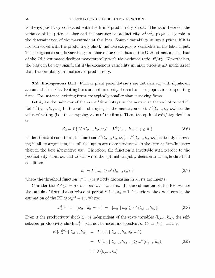
3.2. Endogenous Exit. Firm or plant panel datasets are unbalanced, with signi�cant
amount of �rm exits. Exiting �rms are not randomly chosen from the population of operating
�rms. For instance, existing �rms are typically smaller than surviving �rms.
Let dit be the indicator of the event "�rm i stays in the market at the end of period t".
Let V 1(lit�1; kit; !it) be the value of staying in the market, and let V 0(lit�1; kit; !it) be the
value of exiting (i.e., the scrapping value of the �rm). Then, the optimal exit/stay decision
is:
dit = I�V 1(lit�1; kit; !it)� V 0(lit�1; kit; !it) � 0
(3.6)
Under standard conditions, the function V 1(lit�1; kit; !it)�V 0(lit�1; kit; !it) is strictly increas-ing in all its arguments, i.e., all the inputs are more productive in the current �rm/industry
than in the best alternative use. Therefore, the function is invertible with respect to the
productivity shock !it and we can write the optimal exit/stay decision as a single-threshold
condition:
dit = I f !it � !� (lit�1; kit) g (3.7)
where the threshold function !� (:; :) is strictly decreasing in all its arguments.
Consider the PF yit = �L lit + �K kit + !it + eit. In the estimation of this PF, we use
the sample of �rms that survived at period t: i.e., dit = 1. Therefore, the error term in the
estimation of the PF is !d=1it + eit, where:
!d=1it � f!it j dit = 1g = f!it j !it � !� (li;t�1; kit)g (3.8)
Even if the productivity shock !it is independent of the state variables (li;t�1; kit), the self-
selected productivity shock !d=1it will not be mean-independent of (li;t�1; kit). That is,
E�!d=1it j li;t�1; kit
�= E (!it j li;t�1; kit; dit = 1)
= E (!it j li;t�1; kit; !it � !� (li;t�1; kit))
= � (li;t�1; kit)
(3.9)

3. ECONOMETRIC ISSUES 57
� (li;t�1; kit) is the selection term. Therefore, the PF can be written as:
yit = �L lit + �K kit + � (li;t�1; kit) + ~!it + eit (3.10)
where ~!it � f!d=1it � � (li;t�1; kit)g that, by construction, is mean-independent of (li;t�1; kit).Ignoring the selection term � (li;t�1; kit) introduces bias in our estimates of the PF pa-
rameters. The selection term is an increasing function of the threshold !� (li;t�1; kit), and
therefore it is decreasing in li;t�1 and kit. Both lit and kit are negatively correlated with the
selection term, but the correlation with the capital stock tend to be larger because the value
of a �rm depends strongly on its capital stock than on its "stock" of labor. Therefore, this
selection problem tends to bias downward the estimate of the capital coe¢ cient.
To provide an intuitive interpretation of this bias, �rst consider the case of very large
�rms. Firms with a large capital stock are very likely to survive, even if the �rm receives a
bad productivity shock. Therefore, for large �rms, endogenous exit induces little censoring
in the distribution of productivity shocks. Consider now the case of very small �rms. Firms
with a small capital stock have a large probability of exiting, even if their productivity shocks
are not too negative. For small �rms, exit induces a very signi�cant left-censoring in the
distribution of productivity, i.e., we only observe small �rms with good productivity shocks
and therefore with high levels of output. If we ignore this selection, we will conclude that
�rms with large capital stocks are not much more productive than �rms with small capital
stocks. But that conclusion is partly spurious because we do not observe many �rms with
low capital stocks that would have produced low levels of output if they had stayed.
This type of selection problem has been pointed out also by di¤erent authors who have
studied empirically the relationship between �rm growth and �rm size. The relationship
between �rm size and �rm growth has important policy implications. Mans�eld (1962),
Evans (1987), and Hall (1987) are seminal papers in that literature. Consider the regression
equation:
�sit = �+ � si;t�1 + "it (3.11)
where sit represents the logarithm of a measure of �rm size, e.g., the logarithm of capital
stock, or the logarithm of the number of workers. Suppose that the exit decision at period
t depends on �rm size, si;t�1, and on a shock "it. More speci�cally,
dit = I f "it � "� (si;t�1) g (3.12)
where "� (:) is a decreasing function, i.e., smaller �rms are more likely to exit. In a regression
of �sit on si;t�1, we can use only observations from surviving �rms. Therefore, the regression
of �sit on si;t�1 can be represented using the equation �sit = � + � si;t�1 + "d=1it , where
"d=1it � f"itjdit = 1g = f"itj"it � "� (si;t�1)g. Thus,
�sit = �+ �si;t�1 + � (si;t�1) + ~"it (3.13)

58 3. ESTIMATION OF PRODUCTION FUNCTIONS
where � (si;t�1) � E("itj"it � "� (si;t�1)), and ~"it � f"d=1it �� (li;t�1; kit)g that, by construction,is mean-independent of �rm size at t�1. The selection term � (si;t�1) is an increasing functionof the threshold "� (si;t�1), and therefore it is decreasing in �rm size. If the selection term
is ignored in the regression of �sit on si;t�1, then the OLS estimator of � will be downward
biased. That is, it seems that smaller �rms grow faster just because small �rms that would
like to grow slowly have exited the industry and they are not observed in the sample.
Mans�eld (1962) already pointed out to the possibility of a selection bias due to endoge-
nous exit. He used panel data from three US industries, steel, petroleum, and tires, over
several periods. He tests the null hypothesis of � = 0, i.e., Gibrat�s Law. Using only the sub-
sample of surviving �rms, he can reject Gibrat�s Law in 7 of the 10 samples. Including also
exiting �rms and using the imputed values �sit = �1 for these �rms, he rejects Gibrat�s Lawfor only for 4 of the 10 samples. Of course, the main limitation of Mans�eld�s approach is
that including exiting �rms using the imputed values �sit = �1 does not correct completelyfor selection bias. But Mans�eld�s paper was written almost twenty years before Heckman�s
seminal contributions on sample selection in econometrics. Hall (1987) and Evans (1987)
dealt with the selection problem using Heckman�s two-step estimator. Both authors �nd
that ignoring endogenous exit induces signi�cant downward bias in �. However, they also
�nd that after controlling for endogenous selection a la Heckman, the estimate of � is sig-
ni�cantly lower than zero. They reject Gibrat�s Law. A limitation of their approach is that
their models do not have any exclusion restriction and identi�cation is based on functional
form assumptions, i.e., normality of the error term, and linear relationship between �rm size
and �rm growth.
4. Estimation Methods
4.1. Using Input Prices as Instruments. If input prices, ri, are observable, andthey are not correlated with the productivity shock !i, then we can use these variables
as instruments in the estimation of the PF. However, this approach has several important
limitations. First, input prices are not always observable in some datasets, or they are only
observable at the aggregate level but not at the �rm level. Second, if �rms in our sample
use homogeneous inputs, and operate in the same output and input markets, we should not
expect to �nd any signi�cant cross-sectional variation in input prices. Time-series variation
is not enough for identi�cation. Third, if �rms in our sample operate in di¤erent input
markets, we may observe signi�cant cross-sectional variation in input prices. However, this
variation is suspicious of being endogenous. The di¤erent markets where �rms operate can be
also di¤erent in the average unobserved productivity of �rms, and therefore cov (!i; ri) 6= 0,i.e., input prices not a valid instruments. In general, when there is cross-sectional variability
4. ESTIMATION METHODS 59
in input prices, can one say that input prices are valid instruments for inputs in a PF? Is
cov (!i; ri) = 0? When inputs are �rm-speci�c, it is commonly the case that input prices
depend on the �rm�s productivity.
4.2. Panel Data: Fixed-E¤ects Estimators. Suppose that we have �rm level panel
data with information on output, capital and labor for N �rms during T time periods. The
Cobb-Douglas PF is:
yit = �L lit + �K kit + !it + eit (4.1)
Mundlak (1961) and Mundlak and Hoch (1965) are seminal studies in the use of panel data
for the estimation of production functions. They consider the estimation of a production
function of an agricultural product. They postulate the following assumptions:
Assumption PD-1: !it has the following variance-components structure: !it = �i + �t + !�it.
The term �i is a time-invariant, �rm-speci�c e¤ect that may be interpreted as the quality of
a �xed input such as managerial ability, or land quality. �t is an aggregate shock a¤ecting
all �rms. And !�it is an �rm idiosyncratic shock.
Assumption PD-2: The amount of inputs depend on some other exogenous time varying
variables, such that var�lit � �li
�> 0 and var
�kit � �ki
�> 0, where �li � T�1
PTt=1 lit, and
�ki � T�1PT
t=1 kit.
Assumption PD-3: !�it is not serially correlated.
Assumption PD-4: The idiosyncratic shock !�it is realized after the �rm decides the amount
of inputs to employ at period t. In the context of an agricultural PF, this shock may be
intepreted as weather, or other random and unpredictable shock.
The Within-Groups estimator (WGE) or �xed-e¤ects estimator of the PF is just the OLS
estimator in the Within-Groups transformed equation:
(yit � �yi) = �L�lit � �li
�+ �K
�kit � �ki
�+ (!it � �!i) + (eit � �ei) (4.2)
Under assumptions (PD-1) to (PD-4), the WGE is consistent. Under these assumptions, the
only endogenous component of the error term is the �xed e¤ect �i. The transitory shocks
!�it and eit do not induce any endogeneity problem. The WG transformation removes the
�xed e¤ect �i.
It is important to point out that, for short panels (i.e., T �xed), the consistency of the
WGE requires the regressors xit � (lit; kit) to be strictly exogenous. That is, for any (t; s):
cov (xit; !�is) = cov (xit; eis) = 0 (4.3)
60 3. ESTIMATION OF PRODUCTION FUNCTIONS
Otherwise, the WG-transformed regressors�lit � �li
�and
�kit � �ki
�would be correlated with
the error (!it � �!i). This is why Assumptions (PD-3) and (PD-4) are necessary for theconsistency of the OLS estimator.
However, it is very common to �nd that the WGE estimator provides very small esti-
mates of �L and �K (see Grilliches and Mairesse, 1998). There are at least two factors that
can explain this empirical regularity. First, though Assumptions (PD-2) and (PD-3) may be
plausible for the estimation of agricultural PFs, they are very unrealistic for manufacturing
�rms. And second, the bias induced by measurement-error in the regressors can be exacer-
bated by the WG transformation. That is, the noise-to-signal ratio can be much larger for
the WG transformed inputs than for the variables in levels. To see this, consider the model
with only one input, say capital, and suppose that it is measured with error. We observe
k�it where k�it = kit + e
kit, and e
kit represents measurement error in capital and it satis�es the
classical assumptions on measurement error. In the estimation of the PF in levels we have
that:
Bias(�̂OLSL ) =Cov(k; �)
V ar(k) + V ar(ek)� �L V ar(e
k)
V ar(k) + V ar(ek)(4.4)
If V ar(ek) is small relative to V ar(k), then the (downward) bias introduced by the mea-
surement error is negligible in the estimation in levels. In the estimation in �rst di¤erences
(similar to WGE, in fact equivalent when T = 2), we have that:
Bias(�̂WGEL ) = � �L V ar(�e
k)
V ar(�k) + V ar(�ek)(4.5)
Suppose that kit is very persistent (i.e., V ar(k) is much larger than V ar(�k)) and that
ekit is not serially correlated (i.e., V ar(�ek) = 2 � V ar(ek)). Under these conditions, the
ratio V ar(�ek)=V ar(�k) can be large even when the ratio V ar(ek)=V ar(k) is quite small.
Therefore, the WGE may be signi�cantly downward biased.
4.3. Dynamic Panel Data: GMM Estimation. In the WGE described in previoussection, the assumption of strictly exogenous regressors is very unrealistic. However, we can
relax that assumption and estimate the PF using GMM method proposed by Arellano and
Bond (1991). Consider the PF in �rst di¤erences:
�yit = �L �lit + �K �kit +��t +�!�it +�eit (4.6)
We maintain assumptions (PD-1), (PD-2), and (PD-3), but we remove assumption (PD-3).
Instead, we consider the following assumption.
Assumption PD-5: There are adjustment costs in inputs (at least in one input). More
formally, the reduced form equations for labor and capital are lit = fL(li;t�1; ki;t�1; !it) and
4. ESTIMATION METHODS 61
kit = fK(li;t�1; ki;t�1; !it), respectively, where either li;t�1 or ki;t�1, or both, have non-zero
partial derivatives in fL and fK .
Under these assumptions fli;t�j; ki;t�j; yi;t�j : j � 2g are valid instruments in the PD in�rst di¤erences. Identi�cation comes from the combination of two assumptions: (1) serial
correlation of inputs; and (2) no serial correlation in productivity shocks f!�itg. The presenceof adjustment costs implies that the shadow prices of inputs vary across �rms even if �rms
face the same input prices. This variability in shadow prices can be used to identify PF
parameters. The assumption of no serial correlation in f!�itg is key, but it can be testedusing an LM test (see Arellano and Bond, 1991).
This GMM in �rst-di¤erences approach has also its own limitations. In some applications,
it is common to �nd unrealistically small estimates of �L and �K and large standard errors.
(see Blundell and Bond, 2000). Overidentifying restrictions are typically rejected. Further-
more, the i.i.d. assumption on !�it is typically rejected, and this implies that fxi;t�2; yi;t�2gare not valid instruments. It is well-known that the Arellano-Bond GMM estimator may
su¤er of weak-instruments problem when the serial correlation of the regressors in �rst di¤er-
ences is weak (see Arellano and Bover, 1995, and Blundell and Bond, 1998). First di¤erence
transformation also eliminates the cross-sectional variation in inputs and it is subject to the
problem of measurement error in inputs.
The weak-instruments problem deserves further explanation. For simplicity, consider the
model with only one input, xit. We are interested in the estimation of the PF:
yit = � xit + �i + !�it + eit (4.7)
where !�it and eit are not serially correlated. Consider the following dynamic reduced form
equation for the input xit:
xit = � xi;t�1 + �1 �i + �2 !�it (4.8)
where �, �1, and �2 are reduced form parameters, and � 2 [0; 1] captures the existence ofadjustment costs. The PF in �rst di¤erences is:
�yit = � �xit +�!�it +�eit (4.9)
For simplicity, consider that the number of periods in the panel is T = 3. In this context,
Arellano-Bond GMM estimator is equivalent to Anderson-Hsiao IV estimator (Anderson and
Hsiao, 1981, 1982) where the endogenous regressor �xit is instrumented using xi;t�2. This
IV estimator is:
�̂N =
PNi=1 xi;t�2 �yitPNi=1 xi;t�2 �xit
(4.10)
62 3. ESTIMATION OF PRODUCTION FUNCTIONS
Under the assumptions of the model, we have that xi;t�2 is orthogonal to the error (�!�it +�eit).
Therefore, �̂N identi�es � if the (asymptotic) R-square in the auxiliary regression of �xiton xi;t�2 is not zero.
By de�nition, the R-square coe¢ cient in the auxiliary regression of �xit on xi;t�2 is such
that:
p limR2 =Cov (�xit; xi;t�2)
2
V ar (�xit) V ar (xi;t�2)=
( 2 � 1)2
2 ( 0 � 1) 0(4.11)
where j � Cov (xit; xi;t�j) is the autocovariance of order j of fxitg. Taking into accountthat xit =
�1 �i1�� + �2(!it + � !i;t�1 + �
2 !i;t�2 + :::), we can derive the following expressions
for the autocovariances:
0 =�21 �
2�
(1� �)2+�22 �
2!
1� �2
1 =�21 �
2�
(1� �)2+ �
�22 �2!
1� �2
2 =�21 �
2�
(1� �)2+ �2
�22 �2!
1� �2
(4.12)
Therefore, 0 � 1 = (�22�2!)=(1 + �) and 1 � 2 = �(�22�2!)=(1 + �). The R-square is:
R2 =
���22�
2!
1 + �
�22
��22�
2!
1 + �
� �21 �
2�
(1� �)2+�22 �
2!
1� �2
!
=�2 (1� �)2
2 (1� � + (1 + �) �)
(4.13)
with � � �21�2�=�22�2! � 0. We have a problem of weak instruments and poor identi�cation if
this R-square coe¢ cient is very small. It is simple to verify that this R-square is small both
when adjustment costs are small (i.e., � is close to zero) and when adjustment costs are large
(i.e., � is close to one). When using this IV estimator, large adjustments costs are bad news
for identi�cation because with � close to one the �rst di¤erence �xit is almost iid and it is
not correlated with lagged input (or output) values. What is the maximum possible value
of this R-square? It is clear that this R-square is a decreasing function of �. Therefore, the
maximum R-square occurs for �21�2� = � = 0 (i.e., no �xed e¤ects in the input demand).
Then, R2 = �2 (1� �) =2. The maximum value of this R-square is R2 = 0:074 that occurs
when � = 2=3. This is the upper bound for the R-square, but it is a too optimistic upper
bound because it is based on the assumption of no �xed e¤ects. For instance, a more realistic
case for � is �21�2� = �
22�2! and therefore � = 1. Then, R
2 = �2 (1� �)2 =4. The maximumvalue of this R-square is R2 = 0:016 that occurs when � = 1=2.
4. ESTIMATION METHODS 63
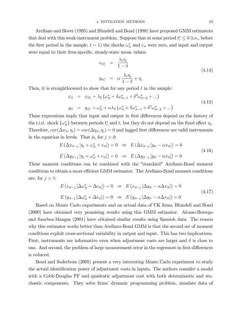
Arellano and Bover (1995) and Blundell and Bond (1998) have proposed GMM estimators
that deal with this weak-instrument problem. Suppose that at some period t�i � 0 (i.e., beforethe �rst period in the sample, t = 1) the shocks !�it and eit were zero, and input and output
were equal to their �rm-speci�c, steady-state mean values:
xit�i =�1�i1� �
yit�i = ��1�i1� � + �i
(4.14)
Then, it is straightforward to show that for any period t in the sample:
xit = xit�i + �2�!�it + �!
�it�1 + �
2!�it�2 + :::�
yit = yit�i + !�it + ��2
�!�it + �!
�it�1 + �
2!�it�2 + :::� (4.15)
These expressions imply that input and output in �rst di¤erences depend on the history of
the i.i.d. shock f!�itg between periods t�i and t, but they do not depend on the �xed e¤ect �i.Therefore, cov(�xit; �i) = cov(�yit; �i) = 0 and lagged �rst di¤erences are valid instruments
in the equation in levels. That is, for j > 0:
E (�xit�j [�i + !�it + eit]) = 0 ) E (�xit�j [yit � �xit]) = 0
E (�yit�j [�i + !�it + eit]) = 0 ) E (�yit�j [yit � �xit]) = 0
(4.16)
These moment conditions can be combined with the "standard" Arellano-Bond moment
conditions to obtain a more e¢ cient GMM estimator. The Arellano-Bond moment conditions
are, for j > 1:
E (xit�j [�!�it +�eit]) = 0 ) E (xit�j [�yit � ��xit]) = 0
E (yit�j [�!�it +�eit]) = 0 ) E (yit�j [�yit � ��xit]) = 0
(4.17)
Based on Monte Carlo experiments and on actual data of UK �rms, Blundell and Bond
(2000) have obtained very promising results using this GMM estimator. Alonso-Borrego
and Sanchez-Mangas (2001) have obtained similar results using Spanish data. The reason
why this estimator works better than Arellano-Bond GMM is that the second set of moment
conditions exploit cross-sectional variability in output and input. This has two implications.
First, instruments are informative even when adjustment costs are larger and � is close to
one. And second, the problem of large measurement error in the regressors in �rst-di¤erences
is reduced.
Bond and Soderbom (2005) present a very interesting Monte Carlo experiment to study
the actual identi�cation power of adjustment costs in inputs. The authors consider a model
with a Cobb-Douglas PF and quadratic adjustment cost with both deterministic and sto-
chastic components. They solve �rms� dynamic programming problem, simulate data of

64 3. ESTIMATION OF PRODUCTION FUNCTIONS
inputs and output using the optimal decision rules, and use simulated data and Blundell-
Bond GMM method to estimate PF parameters. The main results of their experiments
are the following. When adjustment costs have only deterministic components, the iden-
ti�cation is weak if adjustment costs are too low, or too high, or two similar between the
two inputs. With stochastic adjustment costs, identi�cation results improve considerably.
Given these results, one might be tempted to "claim victory": if the true model is such that
there are stochastic shocks (independent of productivity) in the costs of adjusting inputs,
then the panel data GMM approach can identify with precision PF parameters. However,
as Bond and Soderbom explain, there is also a negative interpretation of this result. De-
terministic adjustment costs have little identi�cation power in the estimation of PFs. The
existence of shocks in adjustment costs which are independent of productivity seems a strong
identi�cation condition. If these shocks are not present in the "true model", the apparent
identi�cation using the GMM approach could be spurious because the "identi�cation" would
be due to the misspeci�cation of the model. As we will see in the next section, we obtain a
similar conclusion when using a control function approach.
4.4. Control Function Approaches. In a seminal paper, Olley and Pakes (1996)propose a control function approach to estimate PFs. Levinshon and Petrin (2003) have
extended Olley-Pakes approach to contexts where data on capital investment presents sig-
ni�cant censoring at zero investment.
Consider the Cobb-Douglas PF in the context of the following model of simultaneous
equations:
(PF ) yit = �L lit + �K kit + !it + eit
(LD) lit = fL (li;t�1; kit; !it; rit)
(ID) iit = fK (li;t�1; kit; !it; rit)
(4.18)
where equations (LD) and (ID) represent the �rms�optimal decision rules for labor and capi-
tal investment, respectively, in a dynamic decision model with state variables (li;t�1; kit; !it; rit).
The vector rit represents input prices. Under certain conditions on this system of equations,
we can estimate consistently �L and �K using a control function method.
Olley and Pakes consider the following assumptions:
Assumption OP-1: fK (li;t�1; kit; !it; rit) is invertible in !it.
Assumption OP-2: There is not cross-sectional variation in input prices. For every �rm i,
rit = rt.
Assumption OP-3: !it follows a �rst order Markov process.

4. ESTIMATION METHODS 65
Assumption OP-4: Time-to-build physical capital. Investment iit is chosen at period t but
it is not productive until period t+ 1. And kit+1 = (1� �)kit + iit.
In Olley and Pakes model, lagged labor, li;t�1, is not a state variable, i.e., there a not
labor adjustment costs, and labor is a perfectly �exible input. However, that assumption
is not necessary for Olley-Pakes estimator. Here we discuss the method in the context of a
model with labor adjustment costs.
Olley-Pakes method deals both with the simultaneity problem and with the selection
problem due to endogenous exit. For the sake of clarity, we start describing here a version
of the method that does not deal with the selection problem. We will discuss later their
approach to deal with endogenous exit.
The method proceeds in two-steps. The �rst step estimates �L using a control function
approach, and it relies on assumptions (OP-1) and (OP-2). This �rst step is the same with
and without endogenous exit. The second step estimates �K and it is based on assumptions
(OP-3) and (OP-4). This second step is di¤erent when we deal with endogenous exit.
Step 1: Estimation of �L. Assumptions (OP-1) and (OP-2) imply that !it = f�1K (li;t�1; kit; iit; rt).
Solving this equation into the PF we have:
yit = �L lit + �K kit + f�1L (li;t�1; kit; iit; rt) + eit
= �L lit + �t(li;t�1; kit; iit) + eit
(4.19)
where �t(li;t�1; kit; iit) � �K kit + f�1L (li;t�1; kit; iit; rt). Without a parametric assumption onthe investment equation fK , equation (4.19) is a semiparametric partially linear model. The
parameter �L and the functions �1(:), �2(:), ..., �T (:) can be estimated using semiparametric
methods. A possible semiparametric method is the kernel method in Robinson (1988). In-
stead, Olley and Pakes use polynomial series approximations for the nonparametric functions
�t.
This method is a control function method. Instead of instrumenting the endogenous
regressors, we include additional regressors that capture the endogenous part of the error
term (i.e., proxy for the productivity shock). By including a �exible function in (li;t�1; kit; iit),
we control for the unobservable !it. Therefore, �L is identi�ed if given (li;t�1; kit; iit) there
is enough cross-sectional variation left in lit. The key conditions for the identi�cation of
�L are: (a) invertibility of fL (li;t�1; kit; !it; rt) with respect to !it; (b) rit = rt, i.e., no
cross-sectional variability in unobservables, other than !it, a¤ecting investment; and (c)
given (li;t�1; kit; iit; rt), current labor lit still has enough sample variability. Assumption (c)
is key, and it is the base for Ackerberg, Caves, and Frazer (2006) criticism (and extension)
of Olley-Pakes approach.
66 3. ESTIMATION OF PRODUCTION FUNCTIONS
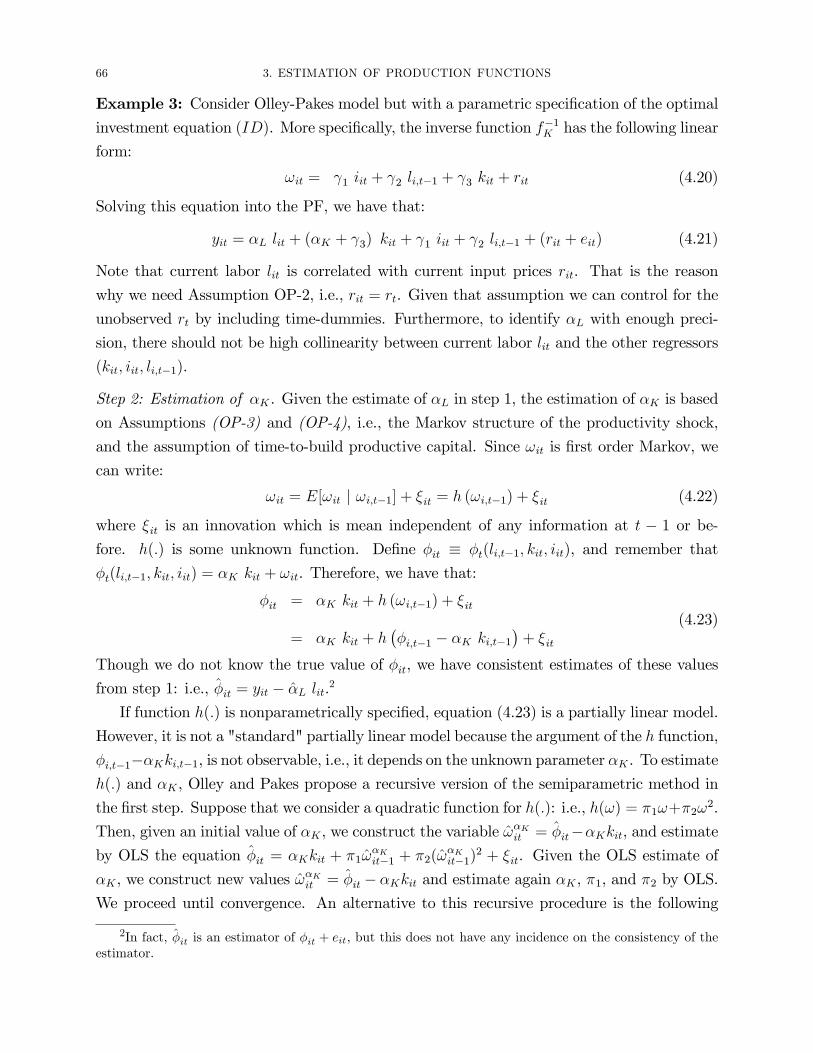
Example 3: Consider Olley-Pakes model but with a parametric speci�cation of the optimalinvestment equation (ID). More speci�cally, the inverse function f�1K has the following linear
form:
!it = 1 iit + 2 li;t�1 + 3 kit + rit (4.20)
Solving this equation into the PF, we have that:
yit = �L lit + (�K + 3) kit + 1 iit + 2 li;t�1 + (rit + eit) (4.21)
Note that current labor lit is correlated with current input prices rit. That is the reason
why we need Assumption OP-2, i.e., rit = rt. Given that assumption we can control for the
unobserved rt by including time-dummies. Furthermore, to identify �L with enough preci-
sion, there should not be high collinearity between current labor lit and the other regressors
(kit; iit; li;t�1).
Step 2: Estimation of �K . Given the estimate of �L in step 1, the estimation of �K is based
on Assumptions (OP-3) and (OP-4), i.e., the Markov structure of the productivity shock,
and the assumption of time-to-build productive capital. Since !it is �rst order Markov, we
can write:
!it = E[!it j !i;t�1] + �it = h (!i;t�1) + �it (4.22)
where �it is an innovation which is mean independent of any information at t � 1 or be-fore. h(:) is some unknown function. De�ne �it � �t(li;t�1; kit; iit), and remember that
�t(li;t�1; kit; iit) = �K kit + !it. Therefore, we have that:
�it = �K kit + h (!i;t�1) + �it
= �K kit + h��i;t�1 � �K ki;t�1
�+ �it
(4.23)
Though we do not know the true value of �it, we have consistent estimates of these values
from step 1: i.e., �̂it = yit � �̂L lit.2
If function h(:) is nonparametrically speci�ed, equation (4.23) is a partially linear model.
However, it is not a "standard" partially linear model because the argument of the h function,
�i;t�1��Kki;t�1, is not observable, i.e., it depends on the unknown parameter �K . To estimateh(:) and �K , Olley and Pakes propose a recursive version of the semiparametric method in
the �rst step. Suppose that we consider a quadratic function for h(:): i.e., h(!) = �1!+�2!2.
Then, given an initial value of �K , we construct the variable !̂�Kit = �̂it��Kkit, and estimate
by OLS the equation �̂it = �Kkit + �1!̂�Kit�1 + �2(!̂
�Kit�1)
2 + �it. Given the OLS estimate of
�K , we construct new values !̂�Kit = �̂it � �Kkit and estimate again �K , �1, and �2 by OLS.
We proceed until convergence. An alternative to this recursive procedure is the following
2In fact, �̂it is an estimator of �it + eit, but this does not have any incidence on the consistency of theestimator.

4. ESTIMATION METHODS 67
Minimum Distance method. For instance, if the speci�cation of h(!) is quadratic, we have
the regression model:
�̂it = �Kkit + �1�̂i;t�1 + �2�̂2
i;t�1 + (��1�K) ki;t�1 + (�2�2K)k2i;t�1
+ (�2�2�K) �̂i;t�1ki;t�1 + �it(4.24)
We can estimate the parameters �K , �1, �2, (��1�K), (�2�2K), and (�2�2�K) by OLS.This estimate of �K can be very imprecise because the collinearity between the regressors.
However, given the estimated vector of f�K , �1, �2, (��1�K), (�2�2K), (�2�2�K)g and itsvariance-covariance matrix, we can obtain a more precise estimate of (�K , �1, �2) by using
minimum distance.
Example 4: Suppose that we consider a parametric speci�cation for the stochastic processof f!itg. More speci�cally, consider the AR(1) process !it = � !i;t�1 + �it, where � 2 [0; 1)is a parameter. Then, h (!i;t�1) = �!i;t�1 = �(�i;t�1 � �K ki;t�1), and we can write:
�it = �K kit + � �i;t�1 + (���K) ki;t�1 + �it (4.25)
we can see that a regression of �it on kit, �i;t�1 and ki;t�1 identi�es (in fact, over-identi�es)
�K and �.
Time-to build is a key assumption for the consistency of this method. If new in-
vestment at period t is productive at the same period, then we have that: �it = �K
ki;t+1 + h��i;t�1 � �K kit
�+ �it. Now, the regressor ki;t+1 depends on investment at period
t and therefore it is correlated with the innovation in productivity �it.
4.5. Ackerberg-Caves-Frazer Critique. Under Assumptions (OP-1) and (OP-2), wecan invert the investment equation to obtain the productivity shock !it = f�1K (li;t�1; kit; iit; rt).
Then, we can solve the expression into the labor demand equation, lit = fL (li;t�1; kit; !it; rt),
to obtain the following relationship:
lit = fL�li;t�1; kit; f
�1K (li;t�1; kit; iit; rt); rt
�= Gt (li;t�1; kit; iit) (4.26)
This expression shows an important implication of Assumptions (OP-1) and (OP-2). For
any cross-section t, there should be a deterministic relationship between employment at
period t and the observable state variables (li;t�1; kit; iit). In other words, once we condition
on the observable variables (li;t�1; kit; iit), employment at period t should not have any cross-
sectional variability. It should be constant. This implies that in the regression in step 1,
yit = �L lit + �t(li;t�1; kit; iit) + eit, it should not be possible to identify �L becuase the
regressor lit does not have any sample variability that is independent of the other regressors
(li;t�1; kit; iit).
68 3. ESTIMATION OF PRODUCTION FUNCTIONS
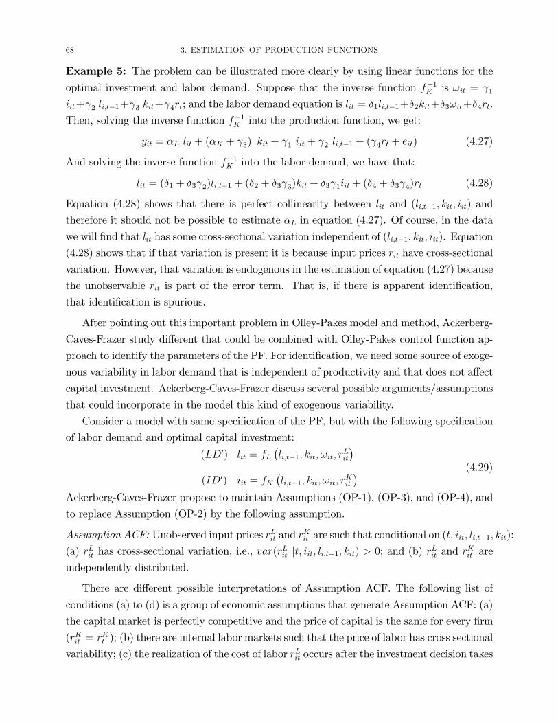
Example 5: The problem can be illustrated more clearly by using linear functions for the
optimal investment and labor demand. Suppose that the inverse function f�1K is !it = 1
iit+ 2 li;t�1+ 3 kit+ 4rt; and the labor demand equation is lit = �1li;t�1+�2kit+�3!it+�4rt.
Then, solving the inverse function f�1K into the production function, we get:
yit = �L lit + (�K + 3) kit + 1 iit + 2 li;t�1 + ( 4rt + eit) (4.27)
And solving the inverse function f�1K into the labor demand, we have that:
lit = (�1 + �3 2)li;t�1 + (�2 + �3 3)kit + �3 1iit + (�4 + �3 4)rt (4.28)
Equation (4.28) shows that there is perfect collinearity between lit and (li;t�1; kit; iit) and
therefore it should not be possible to estimate �L in equation (4.27). Of course, in the data
we will �nd that lit has some cross-sectional variation independent of (li;t�1; kit; iit). Equation
(4.28) shows that if that variation is present it is because input prices rit have cross-sectional
variation. However, that variation is endogenous in the estimation of equation (4.27) because
the unobservable rit is part of the error term. That is, if there is apparent identi�cation,
that identi�cation is spurious.
After pointing out this important problem in Olley-Pakes model and method, Ackerberg-
Caves-Frazer study di¤erent that could be combined with Olley-Pakes control function ap-
proach to identify the parameters of the PF. For identi�cation, we need some source of exoge-
nous variability in labor demand that is independent of productivity and that does not a¤ect
capital investment. Ackerberg-Caves-Frazer discuss several possible arguments/assumptions
that could incorporate in the model this kind of exogenous variability.
Consider a model with same speci�cation of the PF, but with the following speci�cation
of labor demand and optimal capital investment:
(LD0) lit = fL�li;t�1; kit; !it; r
Lit
�(ID0) iit = fK
�li;t�1; kit; !it; r
Kit
� (4.29)
Ackerberg-Caves-Frazer propose to maintain Assumptions (OP-1), (OP-3), and (OP-4), and
to replace Assumption (OP-2) by the following assumption.
Assumption ACF: Unobserved input prices rLit and rKit are such that conditional on (t; iit; li;t�1; kit):
(a) rLit has cross-sectional variation, i.e., var(rLit jt; iit; li;t�1; kit) > 0; and (b) rLit and rKit are
independently distributed.
There are di¤erent possible interpretations of Assumption ACF. The following list of
conditions (a) to (d) is a group of economic assumptions that generate Assumption ACF: (a)
the capital market is perfectly competitive and the price of capital is the same for every �rm
(rKit = rKt ); (b) there are internal labor markets such that the price of labor has cross sectional
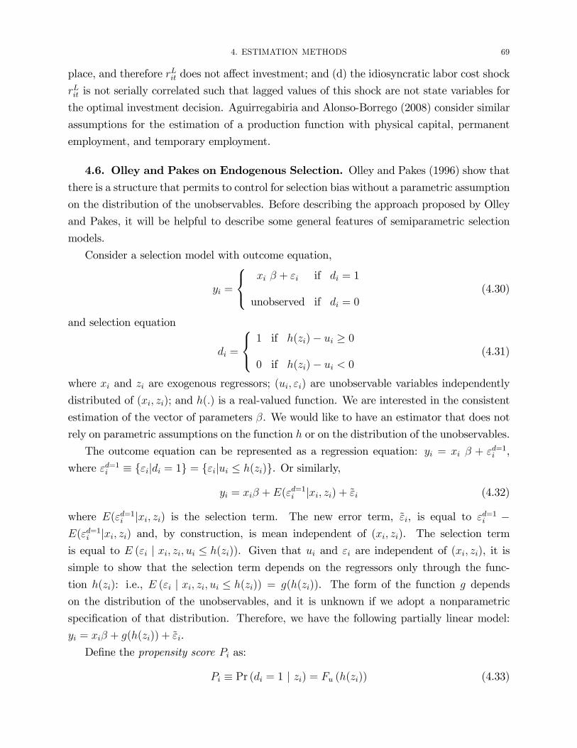
variability; (c) the realization of the cost of labor rLit occurs after the investment decision takes
4. ESTIMATION METHODS 69
place, and therefore rLit does not a¤ect investment; and (d) the idiosyncratic labor cost shock
rLit is not serially correlated such that lagged values of this shock are not state variables for
the optimal investment decision. Aguirregabiria and Alonso-Borrego (2008) consider similar
assumptions for the estimation of a production function with physical capital, permanent
employment, and temporary employment.
4.6. Olley and Pakes on Endogenous Selection. Olley and Pakes (1996) show thatthere is a structure that permits to control for selection bias without a parametric assumption
on the distribution of the unobservables. Before describing the approach proposed by Olley
and Pakes, it will be helpful to describe some general features of semiparametric selection
models.
Consider a selection model with outcome equation,
yi =
8<: xi � + "i if di = 1
unobserved if di = 0(4.30)
and selection equation
di =
8<: 1 if h(zi)� ui � 0
0 if h(zi)� ui < 0(4.31)
where xi and zi are exogenous regressors; (ui; "i) are unobservable variables independently
distributed of (xi; zi); and h(:) is a real-valued function. We are interested in the consistent
estimation of the vector of parameters �. We would like to have an estimator that does not
rely on parametric assumptions on the function h or on the distribution of the unobservables.
The outcome equation can be represented as a regression equation: yi = xi � + "d=1i ,
where "d=1i � f"ijdi = 1g = f"ijui � h(zi)g. Or similarly,
yi = xi� + E("d=1i jxi; zi) + ~"i (4.32)
where E("d=1i jxi; zi) is the selection term. The new error term, ~"i, is equal to "d=1i �E("d=1i jxi; zi) and, by construction, is mean independent of (xi; zi). The selection term
is equal to E ("i j xi; zi; ui � h(zi)). Given that ui and "i are independent of (xi; zi), it issimple to show that the selection term depends on the regressors only through the func-
tion h(zi): i.e., E ("i j xi; zi; ui � h(zi)) = g(h(zi)). The form of the function g depends
on the distribution of the unobservables, and it is unknown if we adopt a nonparametric
speci�cation of that distribution. Therefore, we have the following partially linear model:
yi = xi� + g(h(zi)) + ~"i.
De�ne the propensity score Pi as:
Pi � Pr (di = 1 j zi) = Fu (h(zi)) (4.33)
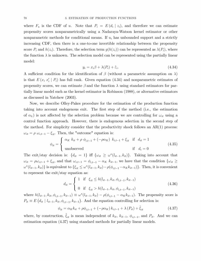
70 3. ESTIMATION OF PRODUCTION FUNCTIONS
where Fu is the CDF of u. Note that Pi = E (di j zi), and therefore we can estimatepropensity scores nonparametrically using a Nadaraya-Watson kernel estimator or other
nonparametric methods for conditional means. If ui has unbounded support and a strictly
increasing CDF, then there is a one-to-one invertible relationship between the propensity
score Pi and h(zi). Therefore, the selection term g(h(zi)) can be represented as �(Pi), where
the function � is unknown. The selection model can be represented using the partially linear
model:
yi = xi� + �(Pi) + ~"i: (4.34)
A su¢ cient condition for the identi�cation of � (without a parametric assumption on �)
is that E (xi x0i j Pi) has full rank. Given equation (4.34) and nonparametric estimates ofpropensity scores, we can estimate � and the function � using standard estimators for par-
tially linear model such as the kernel estimator in Robinson (1988), or alternative estimators
as discussed in Yatchew (2003).
Now, we describe Olley-Pakes procedure for the estimation of the production function
taking into account endogenous exit. The �rst step of the method (i.e., the estimation
of �L) is not a¤ected by the selection problem because we are controlling for !it using a
control function approach. However, there is endogenous selection in the second step of
the method. For simplicity consider that the productivity shock follows an AR(1) process:
!it = � !i;t�1 � �it. Then, the "outcome" equation is:
�it =
8<: �K kit + � �i;t�1 + (���K) ki;t�1 + �it if dit = 1
unobserved if di = 0(4.35)
The exit/stay decision is: fdit = 1g i¤ f!it � !�(lit�1; kit)g. Taking into account that!it = �!i;t�1 + �it, and that !i;t�1 = �i;t�1 � �K kit�1, we have that the condition f!it �!�(lit�1; kit)g is equivalent to f�it � !�(lit�1; kit)��(�i;t�1��Kkit�1)g. Then, it is convenientto represent the exit/stay equation as:
dit =
8<: 1 if �it � h(lit�1; kit; �i;t�1; kit�1)
0 if �it > h(lit�1; kit; �i;t�1; kit�1)(4.36)
where h(lit�1; kit; �i;t�1; kit�1) � !�(lit�1; kit) � �(�i;t�1 � �Kkit�1). The propensity score isPit � E
�dit j lit�1; kit; �i;t�1; kit�1
�. And the equation controlling for selection is:
�it = �Kkit + ��i;t�1 + (���K) ki;t�1 + � (Pit) + ~�it (4.37)
where, by construction, ~�it is mean independent of kit, kit�1, �i;t�1, and Pit. And we can
estimation equation (4.37) using standard methods for partially linear models.
Bibliography
[1] Ackerberg, D., L. Benkard, S. Berry, and A. Pakes (2007): "Econometric Tools for Analyzing MarketOutcomes," Chapter 63 in Handbook of Econometrics, vol. 6A, James J. Heckman and Ed Leamer, eds.North-Holland Press.[2] Ackerberg, D., K. Caves and G. Frazer (2006): "Structural Estimation of Production Functions," man-uscript. Department of Economics, UCLA.[3] Aguirregabiria, V. and Alonso-Borrego, C. (2008): "Labor Contracts and Flexibility: Evidence from aLabor Market Reform in Spain," manuscript. Department of Economics. University of Toronto.[4] Alonso-Borrego, C., and R. Sanchez-Mangas (2001): "GMM Estimation of a Production Function withPanel Data: An Application to Spanish Manufacturing Firms," Statistics and Econometrics Working Papers#015527. Universidad Carlos III.[5] Arellano, M. and S. Bond (1991): "Some Tests of Speci�cation for Panel Data: Monte Carlo Evidenceand an Application to Employment Equations," Review of Economic Studies, 58, 277-297.[6] Arellano, M., and O. Bover (1995): "Another Look at the Instrumental Variable Estimation of Error-Components Models," Journal of Econometrics, 68, 29-51.[7] Blundell, R., and S. Bond (1998): �Initial conditions and moment restrictions in dynamic panel datamodels,�Journal of Econometrics, 87, 115-143.[8] Blundell, R., and S. Bond (2000): �GMM estimation with persistent panel data: an application toproduction functions,�Econometric Reviews, 19(3), 321-340.[9] Bond, S., and M. Söderbom (2005): "Adjustment costs and the identi�cation of Cobb Douglas productionfunctions," IFS Working Papers W05/04, Institute for Fiscal Studies.[10] Bond, S. and J. Van Reenen (2007): "Microeconometric Models of Investment and Employment," in J.Heckman and E. Leamer (editors) Handbook of Econometrics, Vol. 6A. North Holland. Amsterdam.[11] Cobb, C. and P. Douglas (1928): "A Theory of Production," American Economic Review, 18(1), 139-165.[12] Doraszelski, U., and J. Jaumandreu (2013): "R&D and Productivity" Estimating Endogenous Produc-tivity," Review of Economic Studies, forthcoming.[13] Griliches, Z., and J. Mairesse (1998): �Production Functions: The Search for Identi�cation,�in Econo-metrics and Economic Theory in the Twentieth Century: The Ragnar Frisch Centennial Symposium. S.Strøm (editor). Cambridge University Press. Cambridge, UK.[14] Kasahara, H. (2009): �Temporary Increases in Tari¤s and Investment: The Chilean Case,�Journal ofBusiness and Economic Statistics, 27(1), 113-127.[15] Levinshon, J., and A. Petrin (2003): "Estimating Production Functions Using Inputs to Control forUnobservables," Review of Economic Studies , 70, 317-342.[16] Marschak, J. (1953): "Economic measurements for policy and prediction," in Studies in EconometricMethod, eds. W. Hood and T. Koopmans. New York. Wiley.[17] Marshak, J., and W. Andrews (1944): "Random simultaneous equation and the theory of production,"Econometrica, 12, 143�205.[18] Mundlak, Y. (1961): "Empirical Production Function Free of Management Bias," Journal of FarmEconomics, 43, 44-56.[19] Mundlak, Y., and I. Hoch (1965): "Consequences of Alternative Speci�cations in Estimation of Cobb-Douglas Production Functions," Econometrica, 33, 814-828.[20] Olley, S., and A. Pakes (1996): �The Dynamics of Productivity in the Telecommunications EquipmentIndustry�, Econometrica, 64, 1263-97.[21] Pakes, A. (1994): "Dynamic structural models, problems and prospects," in C. Sims (ed.) Advances inEconometrics. Sixth World Congress, Cambridge University Press.
71

72 BIBLIOGRAPHY
[22] Wooldridge, J. (2009): "On Estimating Firm-Level Production Functions Using Proxy Variables toControl for Unobservables," Economics Letters, 104, 112-114.