ESTIMATION OF POROSITY AND FLUID CONSTITUENTS FROM … · define our interactive matrix scale Dfor...

SPWLA 54th

Annual Logging Symposium, June 22-26, 2013

1

ESTIMATION OF POROSITY AND FLUID CONSTITUENTS FROM

NEUTRON AND DENSITY LOGS USING AN INTERACTIVE MATRIX

SCALE

Olabode Ijasan and Carlos Torres-Verdín, The University of Texas at Austin;

William E. Preeg, Consultant

Copyright 2013, held jointly by the Society of Petrophysicists and Well Log

Analysts (SPWLA) and the submitting authors

This paper was prepared for presentation at the SPWLA 54th Annual Logging

Symposium held in New Orleans, Louisiana, June 22-26, 2013.

ABSTRACT

Neutron and density logs are important borehole

measurements for estimating reservoir capacity and

inferring saturating fluids. The neutron log, measuring

hydrogen index (HI), is commonly expressed in

apparent water-filled porosity units assuming a constant

matrix lithology, whereby it is not always

representative of actual pore volume. On the other

hand, a lithology-independent porosity calculation from

nuclear magnetic resonance (NMR) or/and core

measurements, provides reliable evaluations of

reservoir capacity. In practice, not all wells include core

or NMR measurements. The Gaymard-Poupon

calculation of porosity from density and neutron logs,

especially in clean gas-bearing formations, is only an

approximation. This paper introduces an interpretation

workflow wherein formation porosity and hydrocarbon

constituents can be estimated from density and neutron

logs using an interactive, variable matrix scale

specifically suited for the pre-calculated matrix density.

Firstly, we estimate matrix components from

combinations of nuclear logs (photoelectric,

spontaneous gamma ray, neutron, and density) using

Schlumberger’s Nuclear Parameter calculator

(SNUPAR) as a matrix compositional solver while

assuming fresh-water-filled formations. The combined

effects of grain density, volumetric concentration of

shale, matrix-hydrogen, and neutron lithology units

define our interactive matrix scale for correction of

neutron porosity. Under updated matrix conditions, the

resulting neutron-density crossover can only be

attributed to pore volume and saturating fluid effects.

Secondly, porosity, connate-water saturation, and

hydrocarbon density are calculated from the

discrepancy between corrected neutron and density logs

using SNUPAR and Archie’s water saturation equation,

thereby eliminating the assumption of fresh-water

saturation.

With matrix effects eliminated from the neutron-density

overlay, gas- or light-oil-saturated formations,

exhibiting the characteristic gas crossover, are

emphasized to be more representative of saturating

hydrocarbons. This behavior gives a clear qualitative

distinction between hydrocarbon-saturated sweet spots

and non-viable depth zones.

INTRODUCTION

Porosity calculated from neutron and density

measurements is still the most reliable estimate of

reservoir capacity from well-log analysis. In complex

lithologies, inadequate characterization of the matrix

could yield inaccurate porosity and saturation estimates.

The petrophysical effects of lithology, saturating fluid,

and borehole conditions on nuclear logs were

exhaustively discussed by Ellis and Singer (2007).

Using departure curves from log interpretation charts

(Schlumberger, 2009), corrections are applied such that

interpreted properties are representative of the

formation only. Extensive studies and publications on

neutron and density logs, being ubiquitous for porosity

and hydrocarbon estimation, can be found in the

literature.

Historically, total porosity, t, in gas-bearing

formations is approximated with the formula (Gaymard

and Poupon, 1968)

2 2

2

2

N D

t

, (1)

where D and N are density and neutron apparent

porosities, respectively. Mao (2001) studied the

correlation characteristics of D and N for distinct

identification of oil- and gas-saturated zones. Spears

(2006) applied lithofacies-based porosity corrections

derived from neutron-density cross-plots for t

calculations in geologic and reservoir models. Fertl and

Timko (1971) extended the formulations of Gaymard

and Poupon (1968) for calculation of hydrocarbon

density, hc, and detection of oil- and gas-bearing

intervals in shaly sands.

SPWLA 54th


2

The neutron-density overlay technique relies on the

difference between apparent porosities, on a pre-

defined matrix scale, for inferring hydrocarbon

saturation (Shc), t, and hc. Several petrophysical

factors adversely affect the reliability of the overlay

technique. For example, gas detection is challenging in

shaly sands or shale gas reservoirs due to opposite

effects of shale-hydroxyls and gas density in overlay

characteristics. Similarly, in oil-saturated or invaded

gas zones, the decreased difference between neutron

and density apparent porosities masks the

characteristics of light-hydrocarbon crossovers (Mao,

2001). Consequently, application of the overlay

technique requires implementation of a suitable matrix

correction.

In this paper, we estimate Shc, t, and hc using an

interactive analysis workflow based on the neutron-

density overlay technique, with explicit consideration

of neutron matrix scale and shale content. The analysis

workflow improves reliability of the overlay technique

in the presence of arbitrary lithology and fluid effects.

These effects and their influence on neutron and density

apparent porosities are described with a synthetic

example of known lithology and fluid constituents. The

calculated hc enables the differentiation between oil

and gas-saturated intervals when hc < 0.25 g/cm3 and

hc 0.25 g/cm3, respectively, for simplified

interpretation. Our interactive matrix scale method is

applied to field examples of varying geology and

lithology, namely carbonate and shale reservoirs, where

porosity and fluid-saturation estimates are compared to

laboratory core measurements.

INTERPRETATION OF APPARENT POROSITY

FROM NEUTRON AND DENSITY LOGS

The porosity value associated with neutron logs is

inherently apparent for given matrix and fluid units. On

the other hand, compensated bulk density

measurements bear no apparentness until density

porosity is calculated with constant values of matrix

and fluid properties. This is a significant difference

between density and neutron logs.

Density Apparent Porosity – The bulk density

measurement, b, principally responds to formation

electron density such that

,

1

1.0704 0.188M

b e i i

i

V

, (2)

where e,i and Vi are electron density and volume

fraction, respectively, of the i-th component up to M

components. In hydrocarbon-bearing formations, t can

be directly calculated from density logs if and only if

matrix density, m, and fluid density, f, are known

precisely. Otherwise, density apparent porosity, D, is

obtained using

b m

D t D

f m

, (3)

where m and f are assumed matrix and fluid densities,

respectively, e.g. limestone matrix of 2.71 g/cm3 and

fresh-water of 1 g/cm3. The porosity departure, D,

due to m and f assumptions (Ellis and Singer, 2007) is

both qualitatively and quantitatively intuitive such that

2

1b m

D m f m

f mf m

, (4)

where m and f are differences in matrix and fluid

densities, respectively, between assumed and true

properties.

Neutron Apparent Porosity – The neutron log is an

apparent porosity measurement, given that it refers to

an equivalent hydrogen index response in water-filled

lithology units, usually limestone. Limestone unit

implies an equivalent response of water-filled limestone

formation where the pore volume equals that of the

neutron log. As shown by Gaymard and Poupon (1968),

it follows that the environmentally-corrected neutron

porosity log, N, across invaded formations can be

expressed as

1

1 M

N i i t N

imf

HI VHI

, (5)

where HI is hydrogen index, subscript mf identifies

mud filtrate, and N is porosity departure due to

neutron apparent porosity measurement. Equation 5

implies that the neutron response is a superposition of

the volumetric contributions of component hydrogen

concentrations. The apparentness in N is determined

by the neutron porosity unit, usually water-filled

limestone. For example, quartz, calcite, and dolomite

blocks yield N of -2, 0, and 0.5 limestone pu

(porosity units), respectively. This matrix effect is

qualitatively intuitive because quartz and dolomite have

lower and higher matrix densities, respectively, than

limestone. On the other hand, unlike D, the matrix

effect is quantitatively obscure and cannot be calculated

SPWLA 54th


3

directly from equations 3 or 4. This effect is

exacerbated in complex mixtures of various lithologies.

Similarly, a gas-saturated limestone formation yields

negative N because the hydrogen index of gas is

typically lower than that of water.

Hence, a physically intuitive parameter representation

of neutron porosity responses is necessary. Using

neutron characteristic lengths, specifically migration

length, Lm, a calibration of Lm–to–neutron porosity is

used to quantify matrix and lithology response effects

(Ellis and Singer, 2007).

NEUTRON PARAMETER MODEL

The Schlumberger Nuclear Parameter calculator

(SNUPAR, McKeon et al., 1989) calculates nuclear

properties such as Lm, HI, photoelectric factor (PEF),

capture cross section, , etc., for any given mixture of

rocks and fluids. In this paper, we implement Lm for

property characterization of wireline neutron porosity

responses, typically with an AmBe (americium-

beryllium) neutron source. It follows that equation 5

can be re-written as

1N l

m

gL

, (6)

where gl represents the Lm–to–porosity calibration

function in limestone water-filled units; gl is obtained

by fitting a polynomial function to the inverse of

SNUPAR-calculated Lm and limestone pore volume.

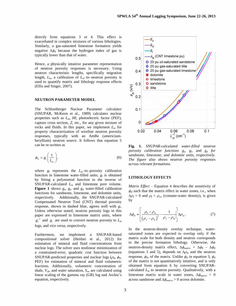
Figure 1 shows gs, gl, and gd water-filled calibration

functions for sandstone, limestone, and dolomite units,

respectively. Additionally, the SNUPAR-calculated

Compensated Neutron Tool (CNT) thermal porosity

response, shown in dashed blue, agrees well with gl.

Unless otherwise stated, neutron porosity logs in this

paper are expressed in limestone matrix units, where 1

lg and lg are used to convert neutron porosity to Lm

logs, and vice versa, respectively.

Furthermore, we implement a SNUPAR-based

compositional solver (Heidari et al., 2012) for

estimation of mineral and fluid concentrations from

nuclear logs. The solver uses nonlinear minimization of

a constrained-error, quadratic cost function between

SNUPAR-predicted properties and nuclear logs (b, N,

PEF) for estimation of mineral and fluid volumetric

fractions. Additionally, volumetric concentration of

shale, Vsh, and water saturation, Sw, are calculated using

linear scaling of the gamma ray (GR) log and Archie’s

equation, respectively.

Fig. 1. SNUPAR-calculated water-filled neutron

porosity calibration functions gs, gl, and gd for

sandstone, limestone, and dolomite units, respectively.

The figure also shows neutron porosity responses

across relevant formations.

LITHOLOGY EFFECTS

Matrix Effect – Equation 4 describes the sensitivity of

D such that the matrix effect in water zones, i.e., when

f = 0 and f = cw (connate-water density), is given

by

2

1b m

D m

f mf m

. (7)

In the neutron-density overlay technique, water-

saturated zones are expected to overlap only if the

matrix scale for both density and neutron corresponds

to the precise formation lithology. Otherwise, the

neutron-density matrix effect, matrix = N - D

(equations 3 and 5), depends on m and the neutron

response, N, of the matrix. Unlike D in equation 3, N

of the matrix is not quantitatively intuitive, and is only

obtained from equation 6 by converting SNUPAR-

calculated Lm to neutron porosity. Qualitatively, with a

limestone matrix scale in water zones, matrix < 0

across sandstone and matrix > 0 across dolomite.

SPWLA 54th


4

Shale-Hydroxyl or Matrix-Hydrogen Effect – Typically,

shales consists of clay minerals with high hydroxyl

(OH–) content such that N > D. The shale-hydroxyl

effect, Nsh, can be approximated from equation 6

using the expression

1Nsh sh l

msh

V gL

, (8)

where Lmsh is SNUPAR-calculated migration length in

shale. For example, Lmsh is approximately 15.35 cm for

illite of density 2.78 g/cm3, whereby Nsh for pure illite

(see Figure 1), i.e., Vsh = 1, corresponds to 0.156. In

unconventional reservoirs with organic-rich kerogen

matrix (Passey et al., 1990), the neutron porosity

response increases due to high hydrogen content of

organic matter. The SNUPAR-calculated HI of kerogen

could be as high as 0.8, depending on both hydrogen-

carbon ratio and kerogen density. Accordingly,

equation 8 quantifies the matrix-hydrogen effect where

Vsh and Lmsh become Vker (volume fraction of kerogen)

and Lmker (SNUPAR-calculated migration length of

kerogen matrix), respectively.

Consequently, the total matrix effect on neutron

porosity logs is an addition of matrix and Nsh, i.e.,

interactive porosity departures due to apparent

limestone matrix scale (calculated from SNUPAR in

fresh-water-filled assumptions, equations 6, and 7) and

shale-hydroxyl or matrix-hydrogen effect (equation 8).

It then follows that the corrected or re-scaled neutron

apparent porosity is given by

Ncorr N matrix Nsh . (9)

FLUID AND HYDROCARBON SATURATION

EFFECTS

Given equations 3, 5, 6, and 9, fluid and saturation

effects on re-scaled neutron apparent porosity can be

written as

1Ncorr t hcS , (10)

where δ is the difference in neutron response between

hydrocarbon-saturated and water-saturated formations.

Several forms of equation 10 are given in Gaymard and

Poupon (1968), Mao (2001), and Quintero et al. (1998).

Gaymard and Poupon (1968) characterized δ across

invaded formations as the relative difference in HI

between residual hydrocarbon and mud-filtrate, i.e.

hc mf mfHI HI HI , (11)

where subscript hc identifies hydrocarbon. For gas-

saturated formations at reservoir conditions, one has

2

9 0.15 0.2 0.9g g gHI

, (12)

where subscript g describes gas. Equation 12 is

replicated in SNUPAR for hc = g < 0.25 g/cm3, while

a SNUPAR-derived functional relationship is obtained

for oil (CnH2n+2) when hc > 0.25 g/cm3. Estimation of

Shc, t, and hc thus requires solving equations 2, 10, 11,

12, and inclusion of a water saturation model, e.g.,

Archie’s equation,

1

w

t nm

t hc

aRR

S

, (13)

where Rt is resistivity log, Rw is connate-water or mud-

filtrate resistivity, a is Archie’s factor, m is porosity

exponent, and n is saturation exponent. It follows that

δ = 0 corresponds to a water or deeply invaded zone.

Consequently, the magnitudes of δ and hc dictate the

hydrocarbon type, i.e., oil or gas.

INTERACTIVE ANALYSIS OF MATRIX AND

FLUID EFFECTS

The interactive analysis involves combined

considerations of petrophysical effects due to apparent

matrix scale and hydrocarbon saturation. Using a

synthetic example of a layered earth model, where well

logs are simulated with UTAPWeLS (The University of

Texas at Austin Petrophysical and Well-Log Simulator,

Voss et al., 2009), we describe the estimation of t, hc,

and Shc using the interactive analysis workflow.

Analysis Workflow – The first part of the analysis

involves matrix compositional interpretation, from b,

PEF, and GR logs, using the SNUPAR-based solver

under the assumption of fresh-water-filled saturation.

We assume fresh-water-filled formations for two

reasons: (1) the environmentally-corrected N is

typically referenced on fresh-water-filled units, and (2)

to independently characterize matrix effects for

estimation of m, given that formation fluids have

negligible or no effect on PEF and GR logs.

Using the estimated m from the matrix solver and

equation 3, we calculate density apparent porosity

under the fresh-water-filled assumption, Dwf.

Accordingly, neutron apparent porosity under the fresh-

water-filled assumption, Nwf, is obtained by converting

predicted Lm from the matrix solver to neutron porosity.

SPWLA 54th


5

It follows from equations 8 and 9 that matrix + Nsh =

Nwf Dwf, i.e. the interactive neutron-density lithology

effect in limestone porosity scale, where Vsh is

calculated assuming linear scaling of the GR log. We

then calculate the corrected neutron apparent porosity,

Ncorr from equation 9 for re-scaling with D. At this

point, the overlay characteristics of Nwf and Dwf are

solely due to porosity effects, while the overlay of Ncorr

and D is due to hydrocarbon pore volume.

The second part of the analysis involves implementing

the SNUPAR-based solver for hydrocarbon

characterization. In this step, equations 2, 10, 11, 12,

and 13 are solved such that a SNUPAR-defined

inherent relationship between δ and hc is implemented

in the analysis for estimation of hc, Shc, and t. The

functional relationship between HI and hc is derived

from SNUPAR for oil (hc > 0.25 g/cm3) and gas (hc <

0.25 g/cm3). Figure 2 summarizes the interpretation

workflow of the interactive analysis.

Fig. 2. Interactive analysis workflow for interpretation

of neutron and density apparent porosities.

Synthetic Example – The interactive analysis workflow

is described for matrix and fluid effects on density and

neutron apparent porosities, using simulated

measurements across a synthetic earth model. Tables 1

and 2 describe the properties assumed for the synthetic

earth model, while Figure 3 shows the simulated

nuclear and resistivity logs. In Figure 4, we describe

the interpretation results obtained with the interactive

analysis workflow. Panels a, f, g, and h show that

estimated m, t, Sw, and hc, respectively, using the

interactive analysis, agree well with model properties in

Table 1. It is particularly significant that the calculated

hc in panel h distinguishes between gas and oil-

saturated layers.

Layers I and IV consist of water-saturated shale of illite

clay, whereby sh = 0.156 and shale density sh = 2.78

g/cm3. After correction for shale-hydroxyl effects, the

actual matrix crossover effect, due to the shale density

greater than limestone density, is shaded in brown in

panel b of Figure 4. On the other hand, layer V consists

of gas-saturated shale, such that the gas crossover effect

becomes accentuated after correction for shale-

hydroxyl effect. In this layer, because gas saturation

and Vsh impose opposite overlay characteristics, N D

experiences a tug between gas and shale-hydroxyl

effects. This behavior in neutron-density interpretation

is especially common in logs acquired across shale gas

formations.

Layers II and III consist of gas- and oil-saturated

limestone formations, respectively. The matrix effect is

irrelevant in these layers because limestone is the

reference scale for neutron-density overlay. This is

corroborated by the overlap of Dwf and Nwf in panel c

of Figure 4. Hydrocarbons, in comparison to fresh

water, reduce the neutron porosity response because of

lower hydrogen index (equation 5). From equations 11

and 12, the hydrocarbon effect is dependent on hc and

is accentuated in gas-saturated layers when compared to

oil-saturated layers. In panels d and e of Figure 4, layer

III shows lower hydrocarbon effects and could be

inadvertently interpreted as a water-filled layer.

Consequently, the fluid solver incorporates the

resistivity measurement, Archie’s model (equation 13),

equations 2, 10, 11, and 12 for an inclusive calculation

of hc, Shc, and t. Panel h shows that the estimated hc

reliably predicts gas and oil densities in gas- and oil-

saturated layers II and III, respectively. In panel f, the t

approximation using Gaymard-Poupon’s formula

(equation 1) is valid in layer II but inaccurate in shaly

layers.

In layers VI and VII, for oil- and water-saturated

dolomite, respectively, the overlay characteristics in

panel b of Figure 4 indicate a matrix crossover. The

matrix effect in panel d shows that matrix = 0.0072

(i.e., 0.72 pu) for sh = 0. By comparison, SNUPAR-

calculated CNT response yields apparent thermal

SPWLA 54th


6

neutron porosity of 0.5 pu in dolomite of 0 % pore

volume.

FIELD EXAMPLES OF APPLICATION

The interactive analysis workflow is implemented for

estimation of m, t, Sw, and hc in two field examples:

(I) gas-bearing carbonate field of dolomite lithology

where m > 2.71 g/cm3, and (II) oil-bearing shale

formation where m < 2.71 g/cm3.

Field Example I, gas-bearing carbonate – This field

example consists of conventional wireline nuclear and

dual induction resistivity logs acquired across a gas-

producing dolomite reservoir. Additionally, the well

includes routine core measurements. Due to low

reservoir pressure, deep mud-filtrate invasion affects

the nuclear logs and even the deep resistivity log, such

that log-derived Shc is considerably lower than in-situ

Shc for water-base mud (Xu et al., 2012). Table 3

summarizes the assumed Archie’s parameters and fluid

properties for the gas-bearing carbonate field.

Figure 5 shows the field measurements, together with

core measurements, compared to results obtained with

the interactive analysis. The neutron-density overlay in

panel b of Figure 5 emphasizes the matrix crossover

because the reservoir is primarily of dolomite lithology.

The gas flag in panel j, proportional to hydrocarbon

pore volume, is most pronounced across XY50 – XY75

ft despite the suppressed gas crossover in panel b.

Across the interval in Figure 5, the gas flag provides a

qualitative and unequivocal indication of hydrocarbon

saturation despite mud-filtrate invasion and matrix

crossover.

The calculated hc in panel h of Figure 5, with a 0.176-

g/cm3 average, confirms that the reservoir is largely

saturated with gas. Conclusively, we implement

combined matrix and fluid volumetric analysis with the

SNUPAR-based solver, where methane gas of 0.176

g/cm3 is assumed as a component of the fluids, thus

eliminating the water-filled assumption in the

independent matrix analysis. Panel i shows cumulative

plot of the volumetric fractions of shale, quartz, calcite,

dolomite, water, and gas, obtained from the SNUPAR-

based solver. The estimated m and t (panels e and f,

respectively), agree well with core measurements. On

the other hand, log-derived Sw (panel g) within interval

XX25 – XY00 ft is considerably lower than core

measurements. This behavior can be attributed to

variations in Archie’s parameters for differing rock

types along the well. Furthermore, Sw in core samples

could increase due to quick spurt loss in low porosity,

low pressure reservoirs (Xu et al., 2012).

Field Example II, oil-bearing shale – In this example,

nuclear and array induction resistivity logs are acquired

in a well, drilled with oil-base mud, across an oil-

bearing shale formation from the Eagle Ford shale play.

Table 4 describes the assumed fluid properties and

Archie’s parameters for the oil-bearing shale reservoir.

Figure 6 shows field measurements, core

measurements, and interpreted petrophysical properties

for the oil-bearing shale example. Here, the SNUPAR-

based matrix analysis assumes kerogen (C100H100O8 of

density 1.4 g/cm3), calcite, kaolinite, and illite as

components of the matrix. Panel e of Figure 6

compares m from the interactive analysis to core

measurements and elemental capture spectroscopy

(ECS) lithology analysis. The ECS-derived m (dashed

blue curve) is significantly larger than core m (blue

circle points). This result is attributed to the exclusion

of low-density kerogen matrix from the ECS analysis.

Matrix density, m from SNUPAR-based matrix

analysis (red curve) agrees well with core

measurements. The resulting fluid crossover, in panel b

of Figure 6, after matrix-hydrogen and shale-hydroxyl

corrections, is due to combined effects of m (less than

2.71 g/cm3 of limestone), fluid density, and fluid

hydrogen index. It is found that the interactive analysis

yields a relatively constant hc of 0.747 g/cm3 for the

interval in panel h. Furthermore, estimated t and Sw

from the interactive analysis (panels f and g,

respectively), agree well with core measurements.

CONCLUSIONS

The interactive analysis workflow re-scales the neutron-

density overlay with corrected neutron and density

apparent porosities in a variable matrix scale, for

independent characterization of fluid effects. It was

found that the SNUPAR-based matrix analysis,

assuming fresh-water-filled formations, renders

accurate estimations of m even across hydrocarbon-

saturated intervals. This result is due to the fact that

formation fluids have negligible or no effect on PEF

and GR logs. One limitation of the SNUPAR-based

matrix analysis is that a priori qualitative knowledge of

matrix components, i.e., lithology, clay mineral, etc., is

essential for accurate estimation of m. This is achieved

by preliminary lithology or matrix identification cross-

plots, such as PEF-b, thorium-potassium, and PEF-

potassium cross-plots (Schlumberger, 2009).

Furthermore, the workflow assumes minimal shoulder-

bed effects such that depth-by-depth analysis is

adequate for SNUPAR calculations.

SPWLA 54th


7

The merits of the SNUPAR-based interactive analysis

workflow include the following: (1) unequivocal

identification of hydrocarbon-saturated zones, (2)

model-consistent formation porosity, and (3)

hydrocarbon density for gas/oil identification. It was

shown that the workflow incorporates interactive matrix

corrections such that the Gaymard-Poupon basis and

formulations for lithology-independent porosity and

hydrocarbon identification can be implemented for any

neutron-density matrix scale and lithology (clean or/and

shaly), especially in wells with limited data.

Synthetic and field examples of application indicate

that lithology-independent porosity and hydrocarbon

density can be efficiently estimated from conventional

nuclear and resistivity logs for reliable and quantitative

detection and appraisal of hydrocarbon-saturated sweet

spots and non-viable zones.

ACKNOWLEDGEMENTS

The work reported in this paper was funded by The

University of Texas at Austin's Research Consortium

on Formation Evaluation, jointly sponsored by Afren,

Anadarko, Apache, Aramco, Baker-Hughes, BG, BHP

Billiton, BP, Chevron, ConocoPhillips, COSL, ENI,

ExxonMobil, Halliburton, Hess, Maersk, Marathon Oil

Corporation, Mexican Institute for Petroleum, Nexen,

ONGC, OXY, Petrobras, Repsol, RWE, Schlumberger,

Shell, Statoil, Total, Weatherford, Wintershall, and

Woodside Petroleum Limited. We are indebted to Shell

Oil Company for providing core and well-log

measurements used in this study.

LIST OF ACRONYMNS AND SYMBOLS

a Archie’s factor

AmBe Americium-beryllium

AO10 10” array induction one foot

resistivity (-m)


resistivity (-m)


resistivity (-m)

CNT Schlumberger compensated neutron

tool

gd Neutron porosity calibration function,

in dolomite units

gl Neutron porosity calibration function,

in limestone units

GR Gamma ray (API)

gs Neutron porosity calibration function,

in sandstone units

HI Hydrogen index ( )

ILD Deep induction resistivity (-m)

ILM Medium induction resistivity (-m)

Lm Neutron migration length (cm)

m Archie’s porosity exponent

M Number of components

n Archie’s saturation exponent

NMR Nuclear magnetic resonance

PEF Photoelectric factor (b/e)

Rt True resistivity (-m)

Rw Water resistivity (-m)

SFLU Spherically focused resistivity (-m)

SNUPAR Schlumberger Nuclear Parameter

calculator

Sw Water saturation (%)

UTAPWeLS The University of Texas at Austin

Petrophysical and Well-Log

Simulator

Vi Volumetric concentration (v/v)

Vsh Volumetric concentration of shale

(v/v)

Capture cross section (cu)

Density (g/cm3)

Departure

Apparent porosity (v/v)

m Matrix density (g/cm3)

t Total porosity (v/v)

δ Neutron fluid effect parameter ( )

Subscripts

b bulk

corr corrected

cw connate-water

D density

e electron

f fluid

g gas

hc hydrocarbon

i component index

ker kerogen

mf mud-filtrate

N neutron

nsh non-shale

sh shale

t total

wf water-filled

REFERENCES

Ellis, D. V. and Singer, J. M., 2007, Well Logging for

Earth Scientists: Springer

SPWLA 54th


8

Fertl, W. H., and Timko, D. J., 1971, “A distinction of

oil and gas in clean and shaly sands as derived from

well logs,” The Log Analyst, vol. 12, no. 2.

Gaymard, R. and Poupon, A., 1968, “Response of

neutron and formation density logs in hydrocarbon

bearing formations,” The Log Analyst, vol. 9, no. 5.

Heidari, Z., Torres-Verdín, C., and Preeg, W. E., 2012,

“Improved estimation of fluid and mineral volumetric

concentrations from well logs in thinly bedded and

invaded formations,” Geophysics, 77(3), WA79-WA98.

Mao, Z., 2001, “The physical dependence and the

correlation characteristics of density and neutron logs,”

Petrophysics, vol. 42, no. 5, 438-443.

McKeon, D. C. and Scott, H. D., 1989, “SNUPAR – A

nuclear parameter code for nuclear geophysics

applications,” IEEE Transactions on Nuclear

Geoscience, vol. 36, no.1, 1215-1219.

Passey, Q. R., Creaney, S., Kulla, J. B., Moretti, F. J.,

and Stroud J. D., 1990, “A practical model for organic

richness from porosity and resistivity logs,” AAPG

Bulletin, vol. 74, no. 12, 1777-1794.

Quintero, L. F., and Bassiouni, Z., 1998, “Porosity

determination in gas-bearing formations,” SPE Permian

Basin Oil and Gas Recovery Conference, March 25-27,

Midland, Texas, SPE 39774.

Schlumberger Limited, 2009, Log Interpretation

Charts: Schlumberger.

Spears, R. W., 2006, “Lithofacies-based corrections to

density-neutron porosity in a high-porosity gas- and oil-

bearing turbidite sandstone reservoir, Erha field, OPL

209, Deepwater Nigeria,” Petrophysics, vol. 47, no. 4,

294-305.

Voss, B., Torres-Verdín, C., Gandhi, A., Alabi, G., and

Lemkecher, M., 2009, “Common stratigraphic

framework to simulate well logs and to cross-validate

static and dynamic petrophysical interpretation,”

SPWLA 50th

Annual Logging Symposium, June 21-24,

The Woodlands, Texas.

Xu, C., Heidari, Z., and Torres-Verdín, C., 2012, “Rock

classification in carbonate reservoirs based on static and

dynamic petrophysical properties estimated from

conventional well logs,” SPE Annual Technical

Conference and Exhibition, October 8-10, San Antonio,

Texas, SPE 159991.

ABOUT THE AUTHORS

Olabode Ijasan is a Ph.D. student in the Department of

Petroleum and Geosystems Engineering at the

University of Texas at Austin, where received an M.Sc.

degree in 2010. He obtained a B.Sc. degree in Electrical

and Electronics Engineering from the University of

Lagos, Nigeria in 2006. In 2011 and 2012, he worked

as a research intern at Schlumberger-Doll Research,

Cambridge, Massachusetts, developing fast and

accurate methods for simulating borehole nuclear

measurements. His research interests include well-log

modeling, inversion, and petrophysical interpretation.

He is a member of SEG, SPE, SPWLA, and IEEE.

Carlos Torres-Verdín received a Ph.D. degree in

Engineering Geoscience from the University of

California, Berkeley, in 1991. Since 1999, he has been

with the Department of Petroleum and Geosystems

Engineering of the University of Texas at Austin, where

he currently hold the position of Zarrow Centennial

Professor in Petroleum Engineering, and director of the

Joint Industry Research Consortium on Formation

Evaluation. He has published more than 114 articles in

refereed technical journals, over 158 articles in

international conferences, and two book chapters. Dr.

Torres-Verdín is co-author of two US patents. He is a

member of the research committee of the SEG and was

a member of the technical committee of the SPWLA

during two terms. He is recipient of the 2003, 2004,

2006, and 2007 Best Paper Award by Petrophysics,

2006 Best Presentation Award and 2007 Best Poster

Awards by the SPWLA, SPWLA’s 2006 Distinguished

Technical Achievement Award, and SPE’s 2008

Formation Evaluation Award.

William E. Preeg received a Ph.D. degree in Nuclear

Science and Engineering from Columbia University in

1970. From 1980 to 2002, he held various positions

with Schlumberger including Director of Research at

Schlumberger-Doll Research (SDR), Vice-president of

Engineering in Houston as well as Manager of the

Nuclear Department at SDR. Prior to 1980, he worked

for Los Alamos Scientific Laboratory, Aerojet Nuclear

Systems Company, and the Atomic Energy

Commission, largely in the area of nuclear radiation

transport. He has also served on advisory committees at

The University of Texas at Austin, Texas A&M,

Colorado School of Mines, and Georgia Tech.

SPWLA 54th


9

Layer Matrix Saturation fluid properties Interpretation comments

I Illite, sh = 2.78 g/cm3

t = 0.10

Sw = 1, Shc = 0 Shale and matrix effects

II Limestone t = 0.28, Sw = 0.05, Shc = 0.95

(Methane, CH4 0.182 g/cm3)

Gas effect

III Limestone t = 0.28, Sw = 0.05, Shc = 0.95

(Oil, C16H34 0.757 g/cm3)

Hydrocarbon effects

IV Illite t = 0.05, Sw = 1, Shc = 0 Shale and matrix effects

V Illite t = 0.10, Sw = 0.20, Shc = 0.80

(Methane, CH4 0.182 g/cm3)

Shale and gas effects

VI Dolomite t = 0.28, Sw = 0.05, Shc = 0.95

(Oil, C16H34 0.757 g/cm3)

Matrix and hydrocarbon

effects

VII Dolomite t = 0.10

Sw = 1, Shc = 0 Matrix effects

VIII Limestone t = 0 Limestone reference

Table 1. Layer properties assumed in the Synthetic Example.

Fig. 3. Simulated well logs across the synthetic multi-layer model. (a) Gamma ray (GR) log, (b) neutron and density

apparent porosities on a limestone scale, (c) array induction apparent resistivity logs, and (d) PEF log. See Table 1

for a description of assumed layer properties.

SPWLA 54th


10

Fig. 4. Interpretation results for the Synthetic Example using the interactive analysis workflow. (a) Interpreted

matrix density from SNUPAR-based matrix solver, (b) neutron-density overlay showing shale-corrected neutron log,

matrix and fluid crossover characteristics, (c) neutron and density apparent water-filled logs from SNUPAR-based

matrix solver, (d) interactive flag indicators showing matrix effect and gas flag, (e) corrected neutron-density

overlay, (f) estimated total porosity, (g) estimated water saturation, and (h) estimated hydrocarbon and fluid

densities. See Table 1 for a description of layer properties.

Variable Value Units

Connate water resistivity, Rw @ 200 °F 0.0203 -m

Connate water density, cw 1.11 g/cm3

Connate water hydrogen index, HIcw 0.936 -

Connate water salt concentration 160,000 ppm NaCl

Archie’s factor, a 1 -

Archie’s porosity exponent, m 1.95 -

Archie’s saturation exponent, n 1.75 -

Table 2. Summary of assumed Archie’s parameters and fluid properties for the Synthetic Example.

SPWLA 54th


11

Fig. 5. Interpretation results for Field Example I, gas-bearing carbonate reservoir, using the interactive analysis

workflow. (a) Gamma ray log, (b) neutron and density porosities on limestone scale, (c) dual-induction resistivity

logs, and (d) photoelectric factor log. (e) Matrix density, (f) total porosity, and (g) water saturation from core

measurements and interactive analysis. (h) Calculated fluid densities showing a gas cut-off of 0.25g/cm3. (i)

Volumetric concentrations of rock and fluid components from SNUPAR-based solver. (j) Gas flag from interactive

analysis workflow.






Mud-filtrate water resistivity, Rmf @ 96 °F 0.84 -m

Mud-filtrate water density, mf 1 g/cm3

Mud-filtrate hydrogen index, HImf 1 -

Mud-filtrate water salt concentration 5147 ppm NaCl



Archie’s saturation exponent, n 1.83 -

Table 3. Summary of assumed fluid properties and Archie’s parameters for Field Example I, gas-bearing carbonate

(Xu et al., 2012).

SPWLA 54th


12

Fig. 6. Interpretation results for Field Example II, oil-bearing shale reservoir, using the interactive analysis

workflow. (a) Gamma ray log, (b) neutron and density porosities on limestone scale, (c) array induction resistivity

logs, and (d) photoelectric factor log. (e) Matrix density, (f) total porosity, and (g) water saturation from core

measurements and interactive analysis. (h) Calculated fluid densities showing a gas cut-off of 0.25g/cm3.








Archie’s saturation exponent, n 2 -

Table 4. Summary of assumed fluid properties and Archie’s parameters for Field Example II, oil-bearing shale.

ESTIMATION OF POROSITY AND FLUID CONSTITUENTS FROM … · define our interactive matrix scale Dfor...

Documents

Transcript of ESTIMATION OF POROSITY AND FLUID CONSTITUENTS FROM … · define our interactive matrix scale Dfor...