ESTIMATION OF PHILLIPS CURVE IN INDIAN CONTEXT … 3 issue 2... · In the case of India, ......

ESTIMATION OF PHILLIPS CURVE IN INDIAN CONTEXT LIPSA RAY

2011 Department of Economics, School of Management,

Pondicherry, University,[email protected] Contact Details LIPSA RAY, C/0- BHABNI BHUSAN RAY, AT-

CHAULIAGANJ, MATHASAHI, PO- NAYABAZAR, DIST- CUTTACK, PIN-753004. ODISSA

Abstract This paper revisits the empirical existence of the Phillips curve in the Indian context. To estimate the Phillips curve we need two variables – inflation and the output gap. In the case of India, incorrect measurement of both variables causes much difficulty in estimating the Phillips curve. I have used Hodrick-Prescott filter approach to find the output gap, ARMA (1) model for expected inflation and finally, used Generalized Method of Moment estimation to estimate the Phillips curve in Indian context. My result shows that the tradeoff between inflation and growth is positive in India during the period of 1970 to 2010. Moreover, I also found that there is no long run relationship between the variables viz; inflation, expected inflation and output gap .Because all the variables are stationary at their original level, which proved that Phillips curve only in short run, not in long run. In long run, it is vertical

1. Introduction The short run relationship between real growth and inflation, which is referred to as Phillips curve (Phillips, 1958) has been the subject of many studies. The rational behind Phillips curve is that as aggregate demand increases, it causes an increase in demand for factors of production, especially labour force pushing wages and employment upward. As wages rise, cost of production rises, leading to higher cost of living. In the long run, economy returns to its long run output and its natural rate of unemployment. For this reason, Phillips curve has been estimated as the short run relationship between unemployment rate and inflation rate. As the former decreases, the latter increases. A Phillips curve is an equation that relates the unemployment rate or some other measure of aggregate economic activity, to a measure of the inflation rate. Modern specifications of Phillips curve equations relate the current rate of unemployment to future changes in the rate of inflation. These specifications are based on the idea that there is a baseline rate of unemployment at which inflation tends to remain constant. The idea is that when unemployment is below this baseline rate, inflation tends to rise over time, and when unemployment is above this rate, inflation tends to fall. The baseline unemployment rate is known as the non-accelerating inflation rate of unemployment (the NAIRU), and modern specifications based on it are known as NAIRU Phillips curves. NAIRU Phillips curves are widely used to produce inflation forecasts, both in the academic literature on inflation forecasting and in policymaking institutions. [1] This wide use is based on the view that inflation forecasts made with these equations are more accurate than forecasts made with other methods. For example, Blinder (1997, p. 241), the former Vice Chairman at the Board of Governors of the Federal Reserve System, argues that "the empirical Phillips curve has worked amazingly well for decades" and concludes, on the basis of this empirical success, that a

Lipsa Ray, Int. J. Eco. Res., 2012, v3i2, 28-51 ISSN: 2229-6158

IJER | MAR - APR 2012 Available [email protected]

28

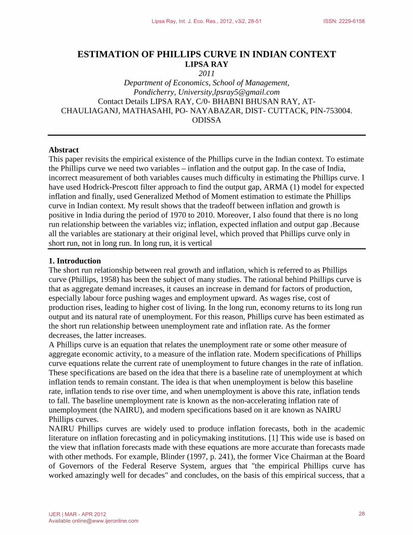
Phillips curve should have "a prominent place in the core model" used for macroeconomic policymaking purposes.

This study critically evaluates the conventional wisdom that NAIRU Phillips curve-based models are useful tools for forecasting inflation. We examine the accuracy of three sets of NAIRU Phillips curve-based inflation forecasts. One set of inflation forecasts is obtained from a simple textbook model of the NAIRU Phillips curve. This textbook model is presented by Stock and Watson (1999b) and others as evidence that the historical data contain a stable negative relationship between the current rate of unemployment and subsequent changes in the rate of inflation which might be exploited to forecast inflation.

Another set of inflation forecasts comes from two NAIRU Phillips curve--based inflation forecasting models similar to those proposed by Stock and Watson (1999a). Their work is a comprehensive study of the accuracy of inflation forecasts from NAIRU Phillips curve--based models and has attracted a great deal of attention, both in the academic literature and in the Federal Reserve System. (See Mankiw 2000 and J. Fisher 2000.) These NAIRU Phillips curve--based models represent the state of the art in the academic inflation forecasting literature.

A third set of forecasts is those produced by the research staff at the Federal Reserve Board of Governors and reported in the Greenbook, the internal collection of materials prepared routinely for meetings of the Federal Open Market Committee. The staff at the Board of Governors uses a large econometric model to help produce the Greenbook forecast. A NAIRU Phillips curve plays a significant role in this model. [2] In particular, the most recent version of the model predicts that, "all else being equal, if the unemployment rate is held 1 percentage point below its equilibrium level on a sustained basis, inflation should climb steadily about 0.4 percentage point a year" (Reifschneider, Tetlow, and Williams 1999, p. 7). The Greenbook forecasts are a key ingredient in the monetary policy debate at the Federal Reserve.

Useful forecasting models exploit stable relationships among variables. Forecasting models that are not based on such stable relationships are not useful because they lead to inaccurate forecasts when the relationships among the variables in the forecasting model change. Do Phillips curves capture stable relationships between unemployment or other measures of economic activity and future inflation? Our review of the evidence indicates that they do not.

Unemployment has been suggested as an indicator of future inflation on the basis of early empirical work documenting a statistical relationship between these variables.

I. Fisher (1926) was the first to document such a relation ship using data from the United States. Later studies by Phillips (1958) and Samuelson and Solow (1960) attracted great attention. These studies all document a negative relationship between the unemployment rate (unemployment as a percentage of the labor force) and either the rate of nominal wage growth or the rate of inflation. Equations relating the unemployment rate to the inflation rate were the first called Phillips curves.

These empirical studies initiated a long debate on the usefulness of Phillips curves for forecasting inflation. Much of this debate has centered on the question of whether the statistical



29

relationship between unemployment and inflation documented in these early empirical studies should be expected to remain stable over time.

Identifying the Phillips curve, which posits a negative relationship between inflation and unemployment, has been of great importance to macroeconomic policymakers. As unemployment is countercyclical, the relationship between inflation and the output gap becomes positive. The empirical accelerationist Phillips curve, which says that the level of inflation is positively related to economic activity, is a robust characteristic of the United States (US) and other developed economies (Gordon, 1977; Phillips, 1958). Explaining the pattern in terms of microeconomic behavior has been, and remains, a key topic of macroeconomic theory (Friedman, 1968; Phelps, 1968; Rudd and Whelan, 2006). Non-inflationary growth has been a major objective of economic planning in India, more so since it was first explicitly stated in the fourth five-year plan (1969-73). In fact, the 1970s saw the emergence of high inflation the world over, and there was a renewed interest in the monetary policy and the role of the central banks in ensuring price stability. In 1991, the Maastricht Treaty marked the consensus of the advanced countries on price stability being the main objective of their central banks. The case of developing countries, including India, has been somewhat different in as much as the central banks have been viewed as responsible not only for price stability but also as facilitators of economic growth. In retrospect, it seems that it has been a job well performed. However, in view of the recent price rise, concerns are being expressed as to why inflation in India is so high. And why is it, that in the case of India, stabilising inflation does not lead to stability in the output gap? Why can’t the Reserve Bank of India (RBI) focus on the single objective of inflation control? The aforesaid questions triggered the present research. To answer these questions, we need to know the empirical relationship between inflation and the output gap - in other words, the Phillips curve. Older Keynesians define the output gap as arising primarily due to inflationary pressures, though the New Keynesian Dynamic Stochastic General Equilibrium theory posits that the output gap arises primarily due to nominal rigidities. The classical model1by Lucas (1973) concludes that the output gap-inflation association is entirely contemporaneous. However, this paper points to the existence of lagged effects, which are difficult to explore in short-term time series. The study concludes that the simple structure of the relationship between inflation and the output gap captures the main phenomenon predicted by the natural rate theory very well.

A theoretical approach to the Phillips curve

In the words of Milton Friedman, “There is always a temporary trade off between inflation and unemployment; there is no permanent trade off. The temporary trade off comes not from inflation per se, but from unanticipated inflation, which generally means, from a rising rate of inflation.” (Richard T. Froyen, Macroeconomics theories and policies, sixth edition) In long run, prices are flexible, the aggregate supply curve is vertical and shifts in aggregate demand affects the price level, not the output level. But in short run, prices are sticky and AS is upward sloping. The short run AS curve implies a trade-off between two measures of economic



30

performance- inflation and unemployment. This trade off called the Phillips curve. The temporary deviation of output from its natural level due to imperfect market causes booms and busts of the business cycle. Y=Yn+α(p-pe) where α>0 Here, Y-output Yn-natural level of output p-price level pe-expected price level when p=pe, Y=Yn

α indicates how much output responds to unexpected changes in the price level. 1/α is the slope of the AS curve (sticky-price). W=wpe

W/p=w/p*pe/p When pe/p=1 or pe=p, W/p=w/p(sticky wage) The Phillips curve in its modern form states that the inflation rate depends on three forces:

• Expected inflation • The deviation of unemployment from the natural rate, called cyclical unemployment • Supply shocks

∏=∏e-β(u-un)+v Here , ∏-inflation ∏e-expected inflation (u-un)-cyclical unemployment v-supply shocks

The minus sign explains higher cyclical unemployment is associated with lower inflation, other things remaining constant. AS curve becomes p=pe+1/α(Y-Yn)+v Here , v is the supply shock to represent exogeneous events such as a change in world oil prices that alter price level and shift the short run AS curve. p-p-1=(pe-p-1)+1/α(Y-Yn)+v here , p-p-1 is the difference between expected price and last year’s price which is expected inflation that is ∏e.

So, ∏=∏e+1/α(Y-Yn)+v Okun’s law states that the deviation of output from its natural level is inversely related to the deviation of unemployment from its natural level that is when output is higher than the natural rate of output, unemployment is lower than the natural rate of unemployment. 1/α(Y-Yn)=-β(u-un)

People form their expectations of inflation based on recently observed inflation. The assumption is called adaptive expectation. For ex: suppose that people expect prices to rise this year at the same rate as they did last year, then expected inflation ∏ e equals last year’s inflation ∏-1.



31

This states that inflation depends on past inflation, cyclical unemployment and a supply shock. When the Phillips curve is written in this form, the natural rate of unemployment is sometimes called the non-accelerating inflation rate of unemployment or NAIRU.

o Cyclical unemployment exerts upward or downward pressure on inflation. Low unemployment pulls the inflation rate up. This is called demand pull inflation because high AD is responsible for this type of inflation. An adverse supply shock such as the rise in world oil prices in 1970s implies a positive value of v and causes inflation to rise. This is called cost push inflation because adverse supply shocks are typically events that push up cost of production. o In the long run, the influence of money is primarily on the price level and other nominal magnitudes. In the long run, real variables, such as real output and employment, are determined by real, not monetary factors. The basis of this proposition is the theory of the natural rate of unemployment and output developed by Milton Friedman. o According to the natural rate theory, there exists an equilibrium level of output and an accompanying rate of unemployment determined by the supply of factors of production, technology and institutions of the economy (real factors). This is Freidman’s natural rate. Changes in AD which Freidman believes are dominated by changes in the supply of money, cause temporary movements of the economy away from natural rate. The monetarists do not agree with the classical position that output is completely supply determined in the short run. o The standard doctrine of Freidman’s Phillips curve is a negative relationship between employment rate and the inflation rate. A high rate of growth in AD stimulates output and hence lowers the unemployment rate. Such high rate of growth in demand also causes an increase in the rate at which price rise (inflation). o Friedman is arguing that the trade-off between inflation and unemployment are rather good in short run because much of the increase in nominal income is in the form of an increase in real output with prices rising to a lesser extent. o Friedman points out that in the short-run product prices increase faster than factor prices, the crucial factor price being the money wage. Thus, the real wage (w/p) falls. This is a necessary condition for output to increase. o When prices have risen, but workers have not yet seen this rise and they will increase labor supply, if offered a higher money wage even if this increase in the money wage is lass than the increase in the price level, even if the real wage is lower. In the short run, labor supply increases because the ex-ante or expected real wage is higher as a result of the higher nominal wage and unchanged view about the behavior of prices. Labor demand increases because of the fall in the ex-post level of the actual real wage paid by the employer. Consequently, unemployment can be pushed below the natural rate. o As suppliers of labor come to anticipate that prices are rising, the Phillips curve will shift upward to the right. Suppliers of labor will demand a high rate of increase in money wages and as a consequence, a high rate of inflation will now correspondents to any given unemployment rate.



32

o Eventually, the policymaker will be led to conclude that inflation has become a more serious problem than unemployment. o In the monetarist view, expansionary monetary policy can only temporarily move the unemployment rate below the natural rate. The long run Phillips curve shows the relationship between inflation and unemployment when expected inflation has time to adjust to the actual inflation rate. When p=pe, that is when inflation is fully adjusted, it becomes vertical. o The theory of the natural rate of unemployment implies that the policymaker can’t peg the unemployment rate at some arbitrarily determined target rate. Attempts to lower the unemployment rate below the natural rate by increasing the rate of growth in AD will be successful only in the short run. The unemployment rate will gradually return to natural rate, and the lasting effect of the expansionary policy will be a higher inflation rate. o In the 1980s, the monetarists saw the high unemployment early in the decade as again the result of previous excessive monetary growth that had created high inflationary expectations. Only after the actual inflation rate fell did the expected inflation rate gradually fall, causing short run Phillips curve to shift downward.

According to Monetarist non-interventionist policy conclusion, the private sector is basically stable if left to itself. Thus, one would not expect large destabilizing shocks to private sector demand for output. Even if there were such shifts in private sector demand, they would have little effect on output, if the money stock were held constant. But Keynesians believe that private sector AD is unstable, primarily because of the instability of investment demand. Keynesians believe that even for a given money stock, such changes in private sector AD can cause large and prolonged fluctuations in income.

Keynesian view:

In the new classical view, systematic monetary and fiscal policy actions that change AD will not affect output and employment even in the short run. That is what has been termed the new classical policy ineffectiveness postulate.

New classical:

Although monetarists question the necessity and desirability of activist policies to affect output and employment and question the effectiveness of fiscal policy actions, they believe that systematic monetary policy actions have real effects in the short run. New classical economists believe that economic agents will form rational expectations. According to the hypothesis of rational expectations, expectations are formed on the basis of all available relevant information concerning the variable being predicted. The individuals use available information intelligently that is they understand the way in which the variables they observe will affect the variable they are trying to predict. A useful contrast can be made between the backward looking nature of expectations in the Keynesian model and the forward looking nature of rational expectations. In the Keynesian



33

model, expectations are backward looking because the expectations of a variable such as the price level adjust to the past behavior of the variable. According to the rational expectation hypothesis, economic agents instead use all available relevant information and intelligently assess the implication of that information for the future behavior of a variable such as price level. According to new classical model, the expected price level depends on Me,ge,te. the new classical view is that there is no useful role for AD policies aimed at stabilizing output and employment. In the case of fiscal policy, new classical economists favor stability and the avoidance of excessive and inflationary stimulus. This paper is divided into 5 sections, including the introduction section. In section 2, I review and discuss the literature on the Phillips curve. Section 3 provides a description on data and methodology used in this study. In section 4, I have shown the empirical results done by using various Econometrics tools. The conclusion part has been included in section 5.

The theory of the Phillips curve was recently proposed in the context of the Indian monetary policy. The report by Rajan (2009) on financial sector reforms recommended that the RBI should focus on the single objective of inflation control, i.e. to stay close to a low inflation rate or to stay within a given range. The report concludes that by doing so, the RBI can achieve stability in growth and inflation. Contradicting the report, Acharya (2009) argued that, given the frequent occurrence of supply shocks in the Indian economy, the single objective of inflation control is not the right choice for the RBI at this stage of development. A monetary response to contain inflation, which is driven by supply-side factors, is ineffective, and in such cases, the RBI has a trade-off between inflation and growth. Singh and Kalirajan (2003) concluded that the ability of central banks in controlling inflation in developing countries is not any better than that of central banks in developed countries. Paul (2009) found empirical evidence for the existence of the Phillips curve for the industrial sector for the longest time period (1956 - 2007). After controlling for agricultural, oil and liberalization shocks, the research proved that the Phillips curve does exist in India, as it does in developed countries. We suspect that the study may perhaps be subject to three major limitations, (a) it accounts only for the industrial sector, which is not a proxy for overall economic activity; (b) it estimates the output gap using the HP method, which is not accurate in the case of developing countries like India; and (c), the author uses the WPI as a measure of inflation which, as discussed above, not capture the demand-side response.

2.Review of Literature:

Another study, Dua and Guar (2009), used quarterly GDP between 1996 and 2005, and after controlling for agricultural shocks and imported inflation through exchange rates, also found a positive relation between the output gap and inflation. In general, a review of the literature on inflation in India suggests that supply shocks were the most prominent issues in India’s inflation dynamics. Therefore, it becomes imperative to appropriately incorporate supply shocks in the estimation of the existence of the Phillips curve in India. In early literature, Poole (1970) argued that the monetary policy objective of stabilisation should focus on both inflation and output. According to Woodford (2003), the recent literature



34

has arrived at a consensus that the objectives of central banks should be to move away from output stabilization and towards the output gap. From an efficiency point of view, and in normal circumstances, the role of output stabilisation means that the central bank intervenes to limit only the output gap. Because the output gap is temporary or short-term deviation from the natural output, the more important role of monetary policy is to focus on the fall or rise in the temporal component of output.

The Phillips curve helps the policymakers decide on policy with inflation and output. Hence, the estimation of the Phillips curve has been applied to economies like the US (Gali and Gertler, 1999; Gordon, 1977; Roberts, 1995; Sbordone, 2002), Australia (Gruen et al., 1999), the UK (Balakrishnan and Lopez-Salido, 2002), Turkey (Domac, 2004), and China (Scheibe and Vines, 2005), in recent years. Rumler (2005) has estimated the new Keynesian Phillips curve (NKPC) for nine euro-area countries: Austria, Belgium, Finland, France, Germany, Greece, Italy, Spain, and the Netherlands. The specialty of the NKPC is that it uses forward-looking expected inflation since prices are sticky by assumption in this model (Roberts, 1995). Bolt and van Els (2000) considered the relationship between the output gap and inflation in various European Union countries as well as Japan and the US. In less-developed economies, the existence of an empirical Phillips curve is often evasive or absent (Bhattacharya, 1984; Dholakia, 1990; IMF, 1996). Many studies, specifically in India, have failed to find the conventional Phillips-curve pattern. In addition, most studies uncovered an unexpected negative relation between inflation and the output gap. The studies that suggest the nonexistence of the Phillips curve for India include Bhalla (1981), Chatterji (1989), Rangarajan (1983), Samanta (1986), Bhattacharya and Lodh (1990), Dholakia (1990), Rangarajan and Arif (1990) and Virmani (2004). Papers in a Phillips-curve framework examine the relation between inflation and the output gap. Out of them, the only paper that explicitly attempts to estimate the Phillips curve for India is Dholakia (1990). Studying a sample from 1950 to 1985, Dholakia asserts that the Indian economy does not seem to face any appreciable tradeoffs between unemployment and inflation even in the short run. He argues that the least-developed countries having underutilized potential would not experience inflationary pressures if the pace of growth is high. Referring to India, Dholakia concludes, ‘‘An imaginary serious tradeoff between inflation and unemployment, in all probability, is not likely to exist.’’ Bhalla (1981) fails to find any evidence of a significantly positive relationship between inflation and excess demand in the Indian economy. Bhalla comments, ‘‘Aggregate changes in real output apparently have no effect on the inflation rate.’’ Studying India’s manufacturing sector over the period from 1961 to 1977, Rangarajan (1983) asserts a negative correlation coefficient between price change and real-output change. Based on Indian yearly data from 1950 to 1988, Bhattacharya and Lodh (1990) find a weak and negative relationship between inflation and output growth. They also refer to Bhattacharya (1984) who argues that the Keynesian Phillips curve does not work in developing countries like India. Ghani (1991) estimates a price equation for India on a sample from 1967 to 1982. The equation shows a negative sign on output. Balakrishnan (1991) works on a sample from 1950 to 1980 in the Indian manufacturing sector. By regressing inflation on the output gap or the ‘activity’



35

variable, Balakrishnan finds a significantly negative relation, which clearly contradicts the Phillips curve for India. In another study on a sample from 1951 to 1990, Nachane and Laxmi (2002) find a negative relation between inflation and the output gap. Brahmananda and Nagaraju (2002) claim that the correlation between inflation and growth, if any, is often negative in Indian data from 1970 to 1999. Using the quarterly data from 1983Q1 to 2001Q4 on output series constructed by Virmani and Kapoor (2003) and Virmani (2004) finds a negative relation between the output gap and inflation. Papers in a Lucas-supply-function framework attempt to see the output gap in response to inflation in India. Following Lucas (1973), Arak (1977) and Makin (1982), one study by Samanta (1986) finds a negative relation between the price level and real output in India. Samanta (1986) attempts to estimate an expectations adjusted supply function (EASF) for India using yearly data from 1952 to 1983. The EASF hypothesis states that price change affects real output or supply only when such price change is purely unanticipated (Lucas, 1973). Samanta’s estimation, which does not justify the EASF for India finds a significantly negative relationship between price surprises and output. Papers in a VAR model examine the interrelationship of output growth, inflation, and money growth in India. Rangarajan and Arif (1990) using annual data over the period from 1961 to 1985 conclude that the price level has no response to the changes in real output. Das (2003) working with money, price, and output of India over the period from April 1992 to March 2000 shows a negative relationship between price and output. Overall most papers, especially papers that clearly focused on the Phillips curve, do not show that a Phillips curve exists for India. A few papers discuss supply shocks faced by India without adequately incorporating them in estimating inflation. Thus, three lines of arguments in explaining inflation dynamics in India can be observed. First, supply shocks are held responsible as a vital factor in determining Indian inflation (Balakrishnan, 1991; Dholakia, 1990; Goyal and Pujari, 2004; Ramachandran, 2004). Second, one group believes that countercyclical money wage is the answer to the negative relation between inflation and the output gap (Ahluwalia, 1979; Balakrishnan, 1991; Roy and Darbha, 2000). Third, another group believes that real marginal cost is not positively correlated with output in India (Chatterji, 1989). Eisenhower’s Fed chairman famously said that his job is to remove the punch bowl as soon as the party really starts to get going. That’s why the 1950s were referred to as the years of the “stop-go” economy. Kennedy, on the other hand, learned the basic power of markets from his supply-side stockbroker father. The dual effect of Kennedy’s tax cuts and that period’s sound money led to what was dubbed the “go-go-economy.” Nixon tried to inflate his way out of stagnation, and then use price controls to put the genie back in the bottle. Gerald Ford tried to use idiotic lapel pins to do the same. It wasn’t until Reagan and Fed chairman Paul Volcker put monetary and fiscal policy into separate categories that the U.S. really started to live up to its economic potential. Alan Greenspan, despite his better training, basically governed the central bank as a Keynesian: Too loose in the late ’80s; too tight in the early ’90s (helping cost George H.W. Bush the election); too tight in the late ’90s in the cause of stopping “irrational exuberance”; and too loose in 2003 because he didn’t believe in the efficacy of the Bush tax cuts.



36

Although economists concluded there wasn’t a long-run tradeoff between inflation and unemployment, they still believed in a short-run effect. From 1979 to 2003, Fed Chairman Paul Volcker and his successor, Alan Greenspan, exploited this method by periodically raising interest rates(the fee paid on borrowed money) to push unemployment higher to achieve lower inflation. In recent years, the Fed and economists have noticed an even further dip in the correlation between unemployment and inflation, even in the short run. During the 1990’s, the unemployment rate fell as low as 3.9% but inflation didn’t materialize. More recent data similar to the 1990’s trend have led economists to look elsewhere for the root of inflation rather than the Phillips curve model that has been used for so long. Rather, the roots of inflation in the macro-economy today are domestic and international competition, and the dismantlement of monopolies which reduce inflation and financial deregulation, the establishment of monopolies and increasing input prices which increase inflation. In a recent paper, Atkeson and Ohanian (2001) challenge the usefulness of the short-run Phillips curve as a tool for forecasting inflation. This Economic Letter summarizes their results and discusses some evidence regarding the empirical instability of the short-run Phillips curve.

Atkeson and Ohanian (2001) argue that, similar to its long-run predecessor, the short-run Phillips curve does not represent a stable empirical relationship that can be exploited for the purpose of constructing reliable inflation forecasts. Their version of the short-run Phillips curve is obtained by regressing the four-quarter change in the inflation rate on the unemployment rate and a constant term. In each quarter, the most recent version of the regression equation is used to construct a forecast of average inflation over the next four quarters.

The Pre–World War I Period: 1861–1913

Phillips begins by analyzing the data for 1861–1913, a time of relative political tranquility and steady, but cyclical, economic expansion in the U.K. Inflfl ation was low and trade unions were in their infancy. In short, this period was uniquely favorable for detecting a stable Phillips curve. Phillips’ scatter plot and curve for this time period, his figure 1, is reproduced here (Figure 1). Phillips plotted “the rate of change of money wage rates” against the unemployment rate. He assumed a constant rate of productivity growth and so the model also explained price inflation, the dependent variable in modern expositions of the Phillips curve. Economists since Hume had sought to explain the determinants of the aggregate price level, primarily via the quantity theory of money. Although there had been some earlier attempts (by Tinbergen, Klein, Hansen, and others) to tackle the rate of change of the price level, Phillips’ work became the paradigm for how economists model inflation.



37

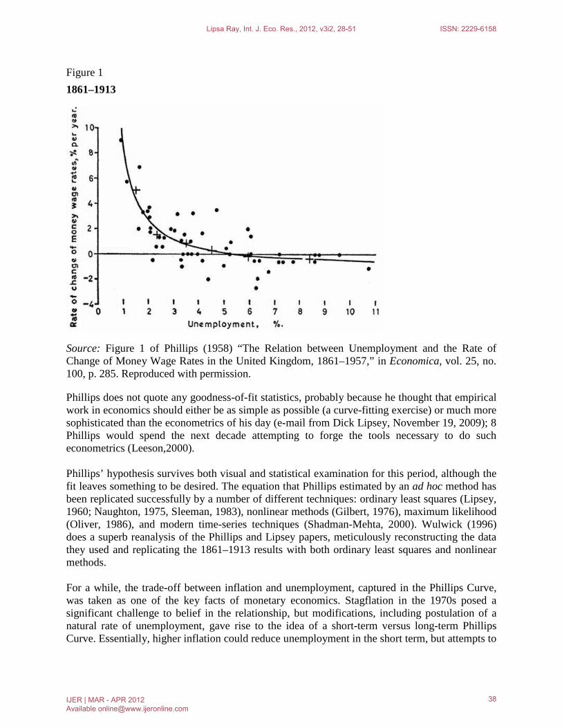
Figure 1 1861–1913

Source: Figure 1 of Phillips (1958) “The Relation between Unemployment and the Rate of Change of Money Wage Rates in the United Kingdom, 1861–1957,” in Economica, vol. 25, no. 100, p. 285. Reproduced with permission.

Phillips does not quote any goodness-of-fit statistics, probably because he thought that empirical work in economics should either be as simple as possible (a curve-fitting exercise) or much more sophisticated than the econometrics of his day (e-mail from Dick Lipsey, November 19, 2009); 8 Phillips would spend the next decade attempting to forge the tools necessary to do such econometrics (Leeson,2000). Phillips’ hypothesis survives both visual and statistical examination for this period, although the fit leaves something to be desired. The equation that Phillips estimated by an ad hoc method has been replicated successfully by a number of different techniques: ordinary least squares (Lipsey, 1960; Naughton, 1975, Sleeman, 1983), nonlinear methods (Gilbert, 1976), maximum likelihood (Oliver, 1986), and modern time-series techniques (Shadman-Mehta, 2000). Wulwick (1996) does a superb reanalysis of the Phillips and Lipsey papers, meticulously reconstructing the data they used and replicating the 1861–1913 results with both ordinary least squares and nonlinear methods. For a while, the trade-off between inflation and unemployment, captured in the Phillips Curve, was taken as one of the key facts of monetary economics. Stagflation in the 1970s posed a significant challenge to belief in the relationship, but modifications, including postulation of a natural rate of unemployment, gave rise to the idea of a short-term versus long-term Phillips Curve. Essentially, higher inflation could reduce unemployment in the short term, but attempts to



38

hold unemployment below its natural rate would lead to increased joblessness and higher inflation over the longer term. Continued empirical investigation into the phenomenon challanged even this notion, however, and there remains disagreement among central bankers over whether there is at any point a reliable relationship between levels of unemployment and rates of inflation. According to Sa Francisco Fed economists Zheng Liu and Glenn Rudebusch, this connection does exist, but only under certain circumstances: “We argue that, in a deep economic downturn such as the current one, inflation and unemployment do tend to move together in a manner consistent with the Phillips curve. But, outside of such severe recessions, fluctuations in the inflation and unemployment rates do not line up particularly well. Inflation appears to be buffeted by many other factors. This explains why some studies find only a "loose empirical relationship" between economic slack and inflation. Thus, compared with the relatively tranquil period between the mid-1980s and the mid-2000s, evidence suggests that recent high unemployment rates are broadly consistent with the sizable decline in core inflation since the fourth quarter of 2007, a relationship that broadly fits the Phillips curve model.”

Paul McCulley, a strategist at PIMCO, a large American fund-management firm, remarks in his latest commentary: “The Fed need not worry that a falling US unemployment rate will quickly generate a rapid acceleration in US wage-driven inflation, as US labour's pricing power is diminished by competition from an augmented global labour supply.” The economist says that The Federal Reserve may focus on the low core rate of inflation but workers may be watching the headline numbers, which in most countries have been significantly higher. The sharp drop in oil prices in recent weeks may reduce this differential, but could easily be reversed by supply disruption or a harsh winter. If workers begin to focus on the effect of higher commodity prices on their spending power, and regard the effect as permanent rather than temporary, then they may push up their wage demands. That could lock higher inflation into the system, giving central banks a devil of a job to bring it back down again. Romar (1993) pointed out that inflation is lower in more open economies, and explained this finding using the time consistency theory of inflation. The most plausible form of the argument ultimately relies on Phillips curves that are steeper in more open economies, and it is precisely this assumption that will be tested below. The correlation between openness and inflation is of wider interest, since the Romer (1993) paper is often considered to be important support for time consistency theories of inflation. Other supportive evidence is lacking, and as romar and Romar (1997,p.310) point out, it is easy to question the generality of the time consistency arguments. The findings in the present paper contribute to this debate.

Here we have used the expectation augmented Phillips curve which shows the relationship of inflation with expected inflation and output gap. This study covers the time period of 1970 to 2010

3.Data and Methodology:



39

So, the equation is ∏t=∏te+β(Y-Yn)+et

Where, ∏t- inflation at a time period t ∏t

e- expected inflation at a time period t Y- actual output (GDP) Yn- potential output et- supply shock (Y-Yn)- outputgap

Data on Wholesale Price Index (WPI), Gross Domestic Product at Factor cost at constant price has been taken from the online database on the Indian economy. Inflation has been calculated as: ((WPIt-WPIt-1)/WPIt-1)*100=∏ The output gap is calculated as the difference between actual GDP and potential GDP which is obtained by the Hodrick-Prescott filter. For expected inflation, we have used adaptive expectation hypothesis which concerntrates upon the past information and the weight of past information keeps on declining.

∏te=α∏t+(1-α)∏e

t-1 By taking 1 period lag in each side, we get ∏e

t-1=α∏t-1+(1-α)∏et-2

∏t=α0+α1∏t-1+ α2∏t-2+………………..+αn∏t-n+et Now, taking expectation on both side, E(∏t)= αe

0+αe1∏t-1+ αe

2∏t-2+………………..+αen∏t-n

For taking appropriate lags, I have used ARMA model. Then I have used Generalised Method of Moment (GMM) estimation to see the relationship between the variables. 4.Empirical Results:

4.1Hodrick-Prescott filter:

The Hodrick-Prescott filter decomposes a time series into growth and cyclical components (Yt=Yt

g+Ytc), where Yt is the natural logarithm of an observed time series and Yt

g and Yt

c are the growth and cyclical components respectively. The filter is given by:

Hodrick and Prescott (1997) minimize the variance of Yt

c subject to a penalty for variations in the second difference of the growth term, where the parameter λ controls the smoothness of Yt

g.3 The minimization of (1) provides a mapping from Yt to Yt

g with Ytc determined residually. The HP

filter is a two-sided filter that is symmetric in the middle of the sample but becomes a one-sided weighted average as we approach either the beginning or the end of the sample. Thus, the HP filter is actually a smoother anywhere in the sample except at the ends where it behaves as a true filter. Since we do not have enough data as we move towards the end of the sample, the HP filter is truncated and becomes nearly asymmetric. More weight is placed on recent observations. Therefore, the HP behaves as a filter at the end of the sample and as a smoother elsewhere.



40

http://www.sciencedirect.com/science?_ob=ArticleURL&_udi=B6V84-3T51RH8-T&_user=2310832&_coverDate=12%2F05%2F1997&_rdoc=1&_fmt=high&_orig=search&_origin=search&_sort=d&_docanchor=&view=c&_acct=C000056865&_version=1&_urlVersion=0&_userid=2310832&md5=1ff1cd596df9658ff98d5ace587591f1&searchtype=a#fn3�

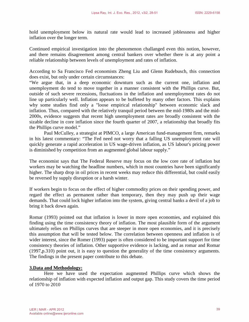
The filter is computed by applying the HP technique with λ equal 100 to real GDP data, running it over a sample from 1970 to 2010.

-150,000

-100,000

-50,000

0

50,000

100,000

150,000

0

1,000,000

2,000,000

3,000,000

4,000,000

1975 1980 1985 1990 1995 2000 2005

GDP Trend Cycle

Hodrick-Prescott Filter (lambda=100)

The gap between the actual GDP and potential GDP gives the output gap. It can be observed that the actual GDP deviates largely during 2000 to 2006. It is due to changes in the growth of GDP. During 2000-2006, the output gap is negative and during 2007-2009, it is positive. By testing ADF test to test the stationarity of the outputgap series, we found that the test statistic is significant because its probability value is less than 0.05 which rejects the null hypothesis i.e YG has a unit root. So, we have to accept the alternative hypothesis i.e YG or outputgap is stationary. Null Hypothesis: YG has a unit root Exogenous: Constant Lag Length: 2 (Automatic based on SIC, MAXLAG=9)

t-Statistic Prob.* Augmented Dickey-Fuller test statistic -3.279490 0.0234

Test critical values: 1% level -3.626784 5% level -2.945842 10% level -2.611531 *MacKinnon (1996) one-sided p-values.



41

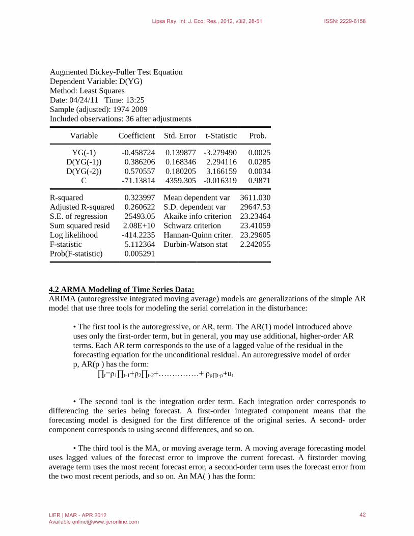
Augmented Dickey-Fuller Test Equation Dependent Variable: D(YG) Method: Least Squares Date: 04/24/11 Time: 13:25 Sample (adjusted): 1974 2009 Included observations: 36 after adjustments

Variable Coefficient Std. Error t-Statistic Prob. YG(-1) -0.458724 0.139877 -3.279490 0.0025

D(YG(-1)) 0.386206 0.168346 2.294116 0.0285 D(YG(-2)) 0.570557 0.180205 3.166159 0.0034

C -71.13814 4359.305 -0.016319 0.9871 R-squared 0.323997 Mean dependent var 3611.030

Adjusted R-squared 0.260622 S.D. dependent var 29647.53 S.E. of regression 25493.05 Akaike info criterion 23.23464 Sum squared resid 2.08E+10 Schwarz criterion 23.41059 Log likelihood -414.2235 Hannan-Quinn criter. 23.29605 F-statistic 5.112364 Durbin-Watson stat 2.242055 Prob(F-statistic) 0.005291

ARIMA (autoregressive integrated moving average) models are generalizations of the simple AR model that use three tools for modeling the serial correlation in the disturbance:

4.2 ARMA Modeling of Time Series Data:

• The first tool is the autoregressive, or AR, term. The AR(1) model introduced above

uses only the first-order term, but in general, you may use additional, higher-order AR terms. Each AR term corresponds to the use of a lagged value of the residual in the forecasting equation for the unconditional residual. An autoregressive model of order p, AR(p ) has the form: ∏t=ρ1∏t-1+ρ2∏t-2+……………+ ρp∏t-p+ut • The second tool is the integration order term. Each integration order corresponds to

differencing the series being forecast. A first-order integrated component means that the forecasting model is designed for the first difference of the original series. A second- order component corresponds to using second differences, and so on.

• The third tool is the MA, or moving average term. A moving average forecasting model

uses lagged values of the forecast error to improve the current forecast. A firstorder moving average term uses the most recent forecast error, a second-order term uses the forecast error from the two most recent periods, and so on. An MA( ) has the form:



42

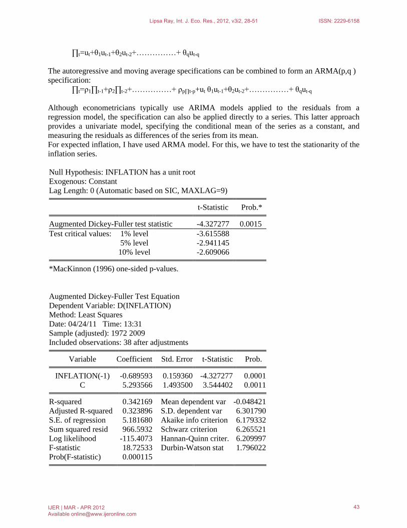
∏t=ut+θ1ut-1+θ2ut-2+……………+ θqut-q

The autoregressive and moving average specifications can be combined to form an ARMA(p,q ) specification: ∏t=ρ1∏t-1+ρ2∏t-2+……………+ ρp∏t-p+ut θ1ut-1+θ2ut-2+……………+ θqut-q

Although econometricians typically use ARIMA models applied to the residuals from a regression model, the specification can also be applied directly to a series. This latter approach provides a univariate model, specifying the conditional mean of the series as a constant, and measuring the residuals as differences of the series from its mean. For expected inflation, I have used ARMA model. For this, we have to test the stationarity of the inflation series. Null Hypothesis: INFLATION has a unit root Exogenous: Constant Lag Length: 0 (Automatic based on SIC, MAXLAG=9)



Augmented Dickey-Fuller Test Equation Dependent Variable: D(INFLATION) Method: Least Squares Date: 04/24/11 Time: 13:31 Sample (adjusted): 1972 2009 Included observations: 38 after adjustments

Variable Coefficient Std. Error t-Statistic Prob. INFLATION(-1) -0.689593 0.159360 -4.327277 0.0001

C 5.293566 1.493500 3.544402 0.0011 R-squared 0.342169 Mean dependent var -0.048421

Adjusted R-squared 0.323896 S.D. dependent var 6.301790 S.E. of regression 5.181680 Akaike info criterion 6.179332 Sum squared resid 966.5932 Schwarz criterion 6.265521 Log likelihood -115.4073 Hannan-Quinn criter. 6.209997 F-statistic 18.72533 Durbin-Watson stat 1.796022 Prob(F-statistic) 0.000115



43

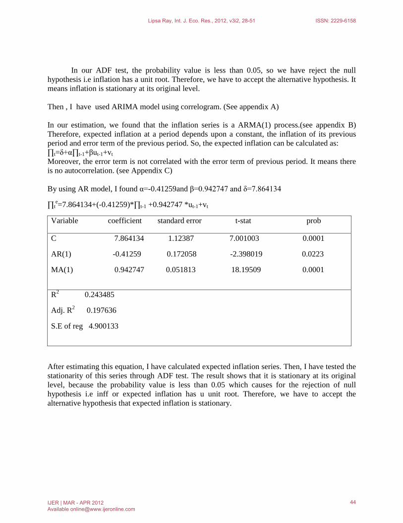
In our ADF test, the probability value is less than 0.05, so we have reject the null hypothesis i.e inflation has a unit root. Therefore, we have to accept the alternative hypothesis. It means inflation is stationary at its original level. Then , I have used ARIMA model using correlogram. (See appendix A) In our estimation, we found that the inflation series is a ARMA(1) process.(see appendix B) Therefore, expected inflation at a period depends upon a constant, the inflation of its previous period and error term of the previous period. So, the expected inflation can be calculated as: ∏t=δ+α∏t-1+βut-1+vt Moreover, the error term is not correlated with the error term of previous period. It means there is no autocorrelation. (see Appendix C) By using AR model, I found α=-0.41259and β=0.942747 and δ=7.864134

∏te=7.864134+(-0.41259)*∏t-1 +0.942747 *ut-1+vt

Variable coefficient standard error t-stat prob

C 7.864134 1.12387 7.001003 0.0001

AR(1) -0.41259 0.172058 -2.398019 0.0223

MA(1) 0.942747 0.051813 18.19509 0.0001

R2 0.243485

Adj. R2 0.197636

S.E of reg 4.900133

After estimating this equation, I have calculated expected inflation series. Then, I have tested the stationarity of this series through ADF test. The result shows that it is stationary at its original level, because the probability value is less than 0.05 which causes for the rejection of null hypothesis i.e inff or expected inflation has u unit root. Therefore, we have to accept the alternative hypothesis that expected inflation is stationary.



44

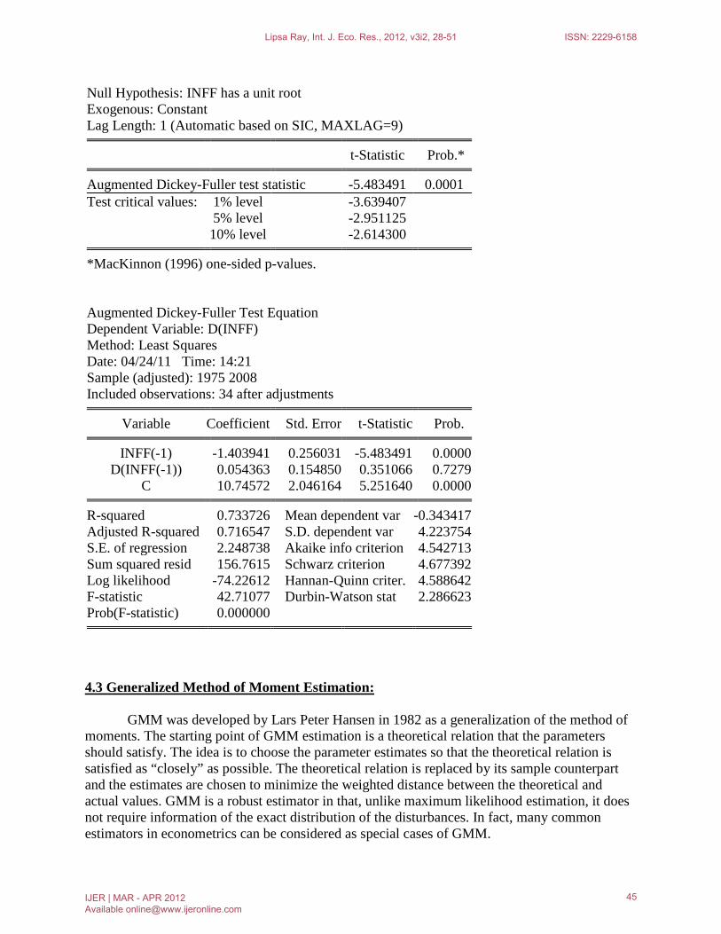
Null Hypothesis: INFF has a unit root Exogenous: Constant Lag Length: 1 (Automatic based on SIC, MAXLAG=9)



Augmented Dickey-Fuller Test Equation Dependent Variable: D(INFF) Method: Least Squares Date: 04/24/11 Time: 14:21 Sample (adjusted): 1975 2008 Included observations: 34 after adjustments

Variable Coefficient Std. Error t-Statistic Prob. INFF(-1) -1.403941 0.256031 -5.483491 0.0000

D(INFF(-1)) 0.054363 0.154850 0.351066 0.7279 C 10.74572 2.046164 5.251640 0.0000 R-squared 0.733726 Mean dependent var -0.343417


GMM was developed by

4.3 Generalized Method of Moment Estimation:

Lars Peter Hansen in 1982 as a generalization of the method of moments. The starting point of GMM estimation is a theoretical relation that the parameters should satisfy. The idea is to choose the parameter estimates so that the theoretical relation is satisfied as “closely” as possible. The theoretical relation is replaced by its sample counterpart and the estimates are chosen to minimize the weighted distance between the theoretical and actual values. GMM is a robust estimator in that, unlike maximum likelihood estimation, it does not require information of the exact distribution of the disturbances. In fact, many common estimators in econometrics can be considered as special cases of GMM.



45

http://en.wikipedia.org/wiki/Lars_Peter_Hansen�

http://en.wikipedia.org/wiki/Method_of_moments_(statistics)�

http://en.wikipedia.org/wiki/Method_of_moments_(statistics)�

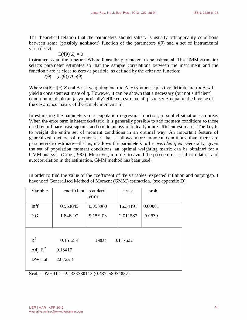
The theoretical relation that the parameters should satisfy is usually orthogonality conditions between some (possibly nonlinear) function of the parameters f(θ) and a set of instrumental variables zt : E(f(θ)’Z) = 0 instruments and the function Where θ are the parameters to be estimated. The GMM estimator selects parameter estimates so that the sample correlations between the instrument and the function f are as close to zero as possible, as defined by the criterion function: J(θ) = (m(θ))’Am(θ) Where m(θ)=f(θ)’Z and A is a weighting matrix. Any symmetric positive definite matrix A will yield a consistent estimate of q. However, it can be shown that a necessary (but not sufficient) condition to obtain an (asymptotically) efficient estimate of q is to set A equal to the inverse of the covariance matrix of the sample moments m. In estimating the parameters of a population regression function, a parallel situation can arise. When the error term is heteroskedastic, it is generally possible to add moment conditions to those used by ordinary least squares and obtain an asymptotically more efficient estimator. The key is to weight the entire set of moment conditions in an optimal way. An important feature of generalized method of moments is that it allows more moment conditions than there are parameters to estimate—that is, it allows the parameters to be overidentified. Generally, given the set of population moment conditions, an optimal weighting matrix can be obtained for a GMM analysis. (Cragg1983). Moreover, in order to avoid the problem of serial correlation and autocorrelation in the estimation, GMM method has been used.

In order to find the value of the coefficient of the variables, expected inflation and outputgap, I have used Generalised Method of Moment (GMM) estimation. (see appendix D)

Variable coefficient standard error

t-stat prob

Inff

YG

0.963845

1.84E-07

0.058980

9.15E-08

16.34191

2.011587

0.00001

0.0530

R2 0.161214 J-stat 0.117622

Adj. R2 0.13417

DW stat 2.072519

Scalar OVERID= 2.4333380113 (0.487458934837)



46

The bracketed value shows the p-value of the chi square test of the J-statistic. Here,the value of the chi square test of J-statistics is 2.43333801113. J-statistics=0.069524.

In the GMM estimation, I found that the value of the coefficient of expected inflation (inff in above table) is significant i.e 0.963845, because the probability value is less than 0.05 which caused the rejection of null hypothesis i.e the value of the coefficient is statistically insignificant. Therefore, we have to accept the alternative hypothesis that the value of the coefficient is statistically significant. The value of the coefficient of output gap (YG in above table) is 1.84E-07. Moreover the Durbin-Watson statistic is close to 2 i.e 1.532508, it means there is no autocorrelation.

Therefore, the equation is stated as follows:

∏t=0.963845*∏t-1+1.84E-07*(Yt-Yn)+Vt

This study has reviewed some recent articles on Phillips Curve in some countries and tried to estimate the relationship between inflation and output growth in Indian economy. I have tried to estimate the Augmented Phillips curve of Indian economy over the period of 1970 to 2010 by taking inflation as dependent variable and expected inflation, outputgap and suuply shock as independent variable. In our ADF test, all the variables are stationary at their original process. It means, they are in I(0) process.

5.Conclusion :

I have used HP filter to find out the level of potential output. After getting potential level of output, output gap has been calculated by deducting potential level of output from actual output i.e GDP at constant price at factor cost. By using ARMA model, I found that inflation at a period depends upon a constant, inflation of its previous period and error term of its previous period, i.e AR(1) and MA(1). By using GMM method, I found that there is positive relationship between inflation and outputgap of Indian economy during 1971-2010. Because, the value of the coefficient of variable outgap is 1.84E-0.7 which shows that with 1 unit change in outputgap, the inflation will change by 1.84E-0.7 units. This positive relationship between inflation and output gap exists only in short-run, because of I(0) process of all the variables. Morever, there is also no relationship between these variables in the long run, because aall the variables viz; inflation, expected inflation and outputgap are stationary at their original level which states that they are not cointegrated.

I have used HP filter which overestimates the potential GDP growth, while it underestimates the potential growth. Therefore, HP method does not yield reliable output gap estimates. Therefore this paper couldn’t give accurate results regarding the existence of Phillips curve and the relationship between its variables. References.



47

A handbook on statistics of Indian Economy, Reserve Bank of India Acharya, S. (2001). India’s macroeconomic management in the 1990s (pp. 1–67). Leading paper

presented at seminar on September 3, 2001. Ten years of economic reform. New Delhi: Indian Council for Research on International Economic Relations

Agarwal, J. D. (2003). Challenges before Indian Economy. Finance India. Indian Institute of Finance., 17(3), 861–865.

Ahluwalia, I. (1979). An analysis of price and output behavior in the Indian economy: 1951–1973. Journal of Development Economics, North-Holland Publishing Company, 6, 353–390.

Arak, M. (1977). Some international evidence on output-inflation trade-offs: Comment. American Economic Review, 67(September), 728–730

Balakrishnan, J., & Lopez-Salido, J. D. (2002). Understanding UK inflation: The role of openness. Bank of England working paper no. 164

Basu. S., Fernald , J.G., (2009). What do we know (and not know) about potential output? Federal Reserve Bank of St. Louis Review 91 (4), 187 - 213.

Biru Paksha Paul Department of Economics, State University of New York at Cortland, 2000, Cortland, NY 13045, United States. Phillips curve Supply and policy shocks, Inflation, Output gap Indian economy.

Chakravarty, S., Chitale, M.P.,Hazari, R.K., Mehta, F.A, Rangarajan, C., and Rao, J.C., (1985). Report of the Committee to Review the Working of the Monetary System. Reserve Bank of India, Bombay, India

Clarida, R., Gali’, J., Gertler, M., (1999). The Science of monetary policy: A new Keynesian perspective. Journal of Economic Literature 37(4), 1661 – 1707

Damodar N. Gujarati, Basic Econometrics, third edition (United States Military Academy, West point

Dua, P., Gaur, U., (2009). Determination of inflation in an open economy Phillips curve framework. Centre for Development Economics, Delhi School of Economics, New Delhi, India. Working Paper No. 178.

Jeffrey M. Wooldridge, Applications of Generalized Method of Moments Estimation, Journal of Economic Perspectives—Volume 15, Number 4—Fall 2001—Pages 87–100

Lucas, Jr. R.E.,(1973). Some international evidence on output-inflation tradeoffs. The American Economic Review 63(3), 361 – 368

Paul, B.P.,(2009). In search of the Phillips curve for India. Journal of Asian Economics 20(4), 479 – 488

Richard T. Froyen, Macroeconomics theories and policies, sixth edition (University of North Carolina at Chapel Hill

Singh, B. K., Kanakaraj, A., & Sridevi, T. O., Revisiting the empirical evidence of Phillips curve of India.

W. Razzak (1998), The Hodrick-Prescott technique: A smoother versus a filter: An application to New Zealand GDP , Reserve Bank of New Zealand, Economics Department, Wellington, New Zealand.

Appendix A



48

http://www.sciencedirect.com/science?_ob=RedirectURL&_method=outwardLink&_partnerName=27983&_origin=article&_zone=art_page&_linkType=scopusAuthorDocuments&_targetURL=http%3A%2F%2Fwww.scopus.com%2Fscopus%2Finward%2Fauthor.url%3FpartnerID%3D10%26rel%3D3.0.0%26sortField%3Dcited%26sortOrder%3Dasc%26author%3DRazzak,%2520W.%26authorID%3D23109529100%26md5%3D5e73a79c5554fa1214688daac7c925f9&_acct=C000056865&_version=1&_userid=2310832&md5=3a80b8bc98c1644c31402012aad1ce62�

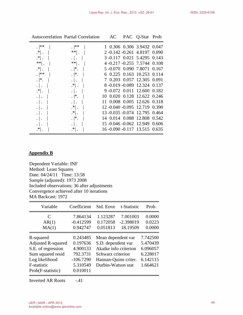
Autocorrelation Partial Correlation AC PAC Q-Stat Prob

. |** | . |** | 1 0.306 0.306 3.9432 0.047

.*| . | **| . | 2 -0.142 -0.261 4.8197 0.090 .*| . | . | . | 3 -0.117 0.021 5.4295 0.143 **| . | **| . | 4 -0.217 -0.255 7.5744 0.108 .*| . | . |*. | 5 -0.070 0.090 7.8071 0.167 . |** | . |*. | 6 0.225 0.163 10.253 0.114 . |*. | . | . | 7 0.203 0.057 12.305 0.091 . | . | .*| . | 8 -0.019 -0.089 12.324 0.137 .*| . | . | . | 9 -0.072 0.011 12.600 0.182 . | . | . |*. | 10 0.020 0.128 12.622 0.246 . | . | . | . | 11 0.008 0.005 12.626 0.318 . | . | .*| . | 12 -0.040 -0.095 12.719 0.390 . | . | .*| . | 13 -0.035 -0.074 12.795 0.464 . | . | . |*. | 14 0.014 0.088 12.808 0.542 . | . | . | . | 15 -0.046 -0.062 12.949 0.606 .*| . | .*| . | 16 -0.090 -0.117 13.515 0.635

Appendix B

Dependent Variable: INF Method: Least Squares Date: 04/24/11 Time: 13:58 Sample (adjusted): 1973 2008 Included observations: 36 after adjustments Convergence achieved after 10 iterations MA Backcast: 1972

Variable Coefficient Std. Error t-Statistic Prob. C 7.864134 1.123287 7.001003 0.0000

AR(1) -0.412599 0.172058 -2.398019 0.0223 MA(1) 0.942747 0.051813 18.19509 0.0000

R-squared 0.243485 Mean dependent var 7.742500


Inverted AR Roots -.41



49

Inverted MA Roots -.94

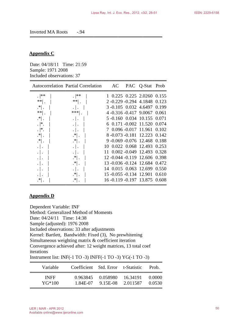
Appendix C

Date: 04/18/11 Time: 21:59 Sample: 1971 2008 Included observations: 37

Autocorrelation Partial Correlation AC PAC Q-Stat Prob . |** | . |** | 1 0.225 0.225 2.0260 0.155

**| . | **| . | 2 -0.229 -0.294 4.1848 0.123 .*| . | . | . | 3 -0.105 0.032 4.6497 0.199 **| . | ***| . | 4 -0.316 -0.417 9.0067 0.061 .*| . | . | . | 5 -0.160 0.034 10.155 0.071 . |*. | . | . | 6 0.171 -0.002 11.520 0.074 . |*. | . | . | 7 0.096 -0.017 11.961 0.102 .*| . | .*| . | 8 -0.073 -0.181 12.223 0.142 .*| . | .*| . | 9 -0.069 -0.076 12.468 0.188 . | . | . | . | 10 0.022 0.068 12.493 0.253 . | . | . | . | 11 0.002 -0.049 12.493 0.328 . | . | .*| . | 12 -0.044 -0.119 12.606 0.398 . | . | .*| . | 13 -0.036 -0.124 12.684 0.472 . | . | . | . | 14 0.015 0.063 12.699 0.550 . | . | .*| . | 15 -0.055 -0.134 12.901 0.610 .*| . | .*| . | 16 -0.119 -0.197 13.875 0.608

Appendix D

Dependent Variable: INF Method: Generalized Method of Moments Date: 04/24/11 Time: 14:38 Sample (adjusted): 1976 2008 Included observations: 33 after adjustments Kernel: Bartlett, Bandwidth: Fixed (3), No prewhitening Simultaneous weighting matrix & coefficient iteration Convergence achieved after: 12 weight matrices, 13 total coef iterations Instrument list: INF(-1 TO -3) INFF(-1 TO -3) YG(-1 TO -3)

Variable Coefficient Std. Error t-Statistic Prob. INFF 0.963845 0.058980 16.34191 0.0000

YG*100 1.84E-07 9.15E-08 2.011587 0.0530



50

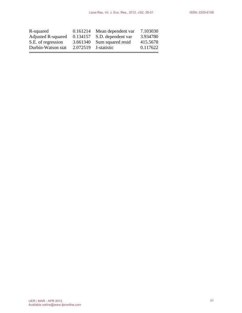
R-squared 0.161214 Mean dependent var 7.103030 Adjusted R-squared 0.134157 S.D. dependent var 3.934780 S.E. of regression 3.661340 Sum squared resid 415.5678 Durbin-Watson stat 2.072519 J-statistic 0.117622



51

ESTIMATION OF PHILLIPS CURVE IN INDIAN CONTEXT … 3 issue 2... · In the case of India, ......

Documents

Transcript of ESTIMATION OF PHILLIPS CURVE IN INDIAN CONTEXT … 3 issue 2... · In the case of India, ......