Estimation of KL Divergence: Optimal Minimax...

Estimation of KL Divergence: Optimal Minimax Rate

Yuheng Bu? Shaofeng Zou ? Yingbin Liang † Venugopal V. Veeravalli ?

? University of Illinois at Urbana-Champaign† Syracuse University

Email: [email protected], [email protected], [email protected], [email protected]

Abstract

The problem of estimating the Kullback-Leibler divergence D(P‖Q) between two unknown distribu-tions P and Q is studied, under the assumption that the alphabet size k of the distributions can scaleto infinity. The estimation is based on m independent samples drawn from P and n independent sam-ples drawn from Q. It is first shown that there does not exist any consistent estimator that guaranteesasymptotically small worst-case quadratic risk over the set of all pairs of distributions. A restricted setthat contains pairs of distributions, with density ratio bounded by a function f(k) is further considered.An augmented plug-in estimator is proposed, and is shown to be consistent if and only if m has an ordergreater than k∨ log2(f(k)), and n has an order greater than kf(k). Moreover, the minimax quadratic risk

is characterized to be within a constant factor of ( km log k

+ kf(k)n log k

)2 + log2 f(k)m

+ f(k)n

, if m and n exceedsa constant factor of k/ log(k) and kf(k)/ log k, respectively. The lower bound on the minimax quadraticrisk is characterized by employing a generalized Le Cam’s method. A minimax optimal estimator is thenconstructed by employing both the polynomial approximation and plug-in approaches.

1 Introduction

As an important quantity in information theory, the Kullback-Leibler (KL) divergence between two distri-butions has a wide range of applications in various domains. For example, KL divergence can be used as asimilarity measure in nonparametric outlier detection [2], multimedia classification [3], text classification [4],and the two-sample problem [5]. In these contexts, it is often desired to estimate KL divergence efficientlybased on available data samples. This paper studies such a problem.

Consider the estimation of KL divergence between two probability distributions P and Q defined as

D(P‖Q) =

k∑i=1

Pi logPiQi, (1)

where P and Q are supported on a common alphabet set [k] , {1, . . . , k}, and P is absolutely continuouswith respect to Q, i.e., if Qi = 0, Pi = 0, for 1 ≤ i ≤ k. We useMk to denote the collection of all such pairsof distributions.

Suppose P and Q are unknown, and that m independent and identically distributed (i.i.d.) samplesX1, . . . , Xm drawn from P and n i.i.d. samples Y1, . . . , Yn drawn from Q are available for estimation.The sufficient statistics for estimating D(P‖Q) are the histograms of the samples M , (M1, . . . ,Mk) andN , (N1, . . . , Nk), where

Mj =

m∑i=1

1{Xi=j} and Nj =

n∑i=1

1{Yi=j} (2)

This work was presented in part at the International Symposium on Information Theory (ISIT), Barcelona, Spain, July2016 [1].

The first two authors have contributed equally to this work.

The work of Y. Bu and V. V. Veeravalli was supported by the National Science Foundation under grants NSF 11-11342 and1617789, through the University of Illinois at Urbana-Champaign. The work of S. Zou and Y. Liang was supported by the AirForce Office of Scientific Research under grant FA 9550-16-1-0077. The work of Y. Liang was also supported by the NationalScience Foundation under Grant CCF-16-17789.

1

record the numbers of occurrences of j ∈ [k] in samples drawn from P and Q, respectively. Then M ∼Multinomial (m,P ) and N ∼ Multinomial (n,Q). An estimator D of D(P‖Q) is then a function of thehistograms M and N , denoted by D(M,N).

We adopt the following worst-case quadratic risk to measure the performance of estimators of the KLdivergence:

R(D, k,m, n) , sup(P,Q)∈Mk

E[(D(M,N)−D(P‖Q))2]. (3)

We further define the minimax quadratic risk as:

R∗(k,m, n) , infDR(D, k,m, n). (4)

In this paper, we are interested in the large-alphabet regime with k → ∞. Furthermore, the number mand n of samples are functions of k, which are allowed to scale with k to infinity.

Definition 1. A sequence of estimators D, indexed by k, is said to be consistent under sample complexitym(k) and n(k) if

limk→∞

R(D, k,m, n) = 0. (5)

We are also interested in the following set:

Mk,f(k) =

{(P,Q) : |P | = |Q| = k,

PiQi≤ f(k), ∀ 1 ≤ i ≤ k

}, (6)

which contains distributions (P,Q) with density ratio bounded by f(k). We define the worst-case quadraticrisk over Mk,f(k) as

R(D,k,m, n, f(k)) , sup(P,Q)∈Mk,f(k)

E[(D(M,N)−D(P‖Q))2], (7)

and define the corresponding minimax quadratic risk as

R∗(k,m, n, f(k)) , infDR(D, k,m, n, f(k)). (8)

1.1 Notations

We adopt the following notation to express asymptotic scaling of quantities with n: f(n) . g(n) representsthat there exists a constant c s.t. f(n) ≤ cg(n); f(n) & g(n) represents that there exists a constant c s.t.f(n) ≥ cg(n); f(n) � g(n) when f(n) & g(n) and f(n) . g(n) hold simultaneously; f(n)� g(n) representsthat for all c > 0, there exists n0 > 0 s.t. for all n > n0, |f(n)| ≥ c|g(n)|; and f(n) � g(n) represents thatfor all c > 0, there exists n0 > 0 s.t. for all n > n0, |f(n)| ≤ cg(n).

1.2 Comparison to Related Problems

Several estimators of KL divergence when P and Q are continuous have been proposed and shown tobe consistent. The estimator proposed in [6] is based on data-dependent partition on the densities, theestimator proposed in [7] is based on a k-nearest neighbor approach, and the estimator developed in [8]utilizes a kernel-based approach for estimating the density ratio. A more general problem of estimating thef -divergence was studied in [9], where an estimator based on a weighted ensemble of plug-in estimators wasproposed to trade bias with variance. All of these approaches exploit the smoothness of continuous densitiesor density ratios, which guarantees that samples falling into a certain neighborhood can be used to estimatethe local density or density ratio accurately. However, such a smoothness property does not hold for discretedistributions, whose probabilities over adjacent point masses can vary significantly. In fact, an example is

2

provided in [6] to show that the estimation of KL divergence can be difficult even for continuous distributionsif the density has sharp dips.

Estimation of KL divergence when the distributions P and Q are discrete has been studied in [10–12] forthe regime with fixed alphabet size k and large sample sizes m and n. Such a regime is very different fromthe large-alphabet regime in which we are interested, with k scaling to infinity. Clearly, as k increases, thescaling of the sample sizes m and n must be fast enough with respect to k in order to guarantee consistentestimation.

In the large-alphabet regime, KL divergence estimation is closely related to entropy estimation with alarge alphabet recently studied in [13–16]. Compared to entropy estimation, KL divergence estimation hasone more dimension of uncertainty, that is regarding the distribution Q. Some distributions Q can containvery small point masses that contribute significantly to the value of divergence, but are difficult to estimatebecause samples of these point masses occur rarely. In particular, such distributions dominate the risk in(3), and make the construction of consistent estimators challenging.

1.3 Summary of Main Results

We summarize our main results in the following three theorems, whose detailed proofs are given respectivelyin Sections 2, 3 and 4.

Our first result, based on Le Cam’s two-point method [17], is that there is no consistent estimator of KLdivergence over the distribution set Mk.

Theorem 1. For any m,n ∈ N, and k ≥ 2, R∗(k,m, n) is infinite. Therefore, there does not exist anyconsistent estimator of KL divergence over the set Mk.

The intuition behind this result is that the set Mk contains distributions Q, that have arbitrarily smallcomponents that contribute significantly to KL divergence but require arbitrarily large number of samplesto estimate accurately. However, in practical applications, it is reasonable to assume that the ratio of P toQ is bounded. Thus, we further focus on the setMk,f(k) given in (6) that contains distribution pairs (P,Q)with their density ratio bounded by f(k).

We construct an augmented plug-in estimator, and characterize the sufficient and necessary conditions onthe sample complexity such that the estimator is consistent in the following theorem.

Theorem 2. The augmented plug-in estimator of KL divergence is consistent over the set Mk,f(k) if andonly if

m� k ∨ log2(f(k)) and n� kf(k). (9)

Our proof of the sufficient conditions is based on evaluating the bias and variance of the estimator sepa-rately. Our proof of the necessary condition m � log2 f(k) is based on Le Cam’s two-point method with ajudiciously chosen pair of distributions. And our proof of the necessary conditions m � k and n � kf(k)is based on analyzing the bias of the estimator and constructing different pairs of “worst case” distributionsfor the cases where either the bias caused by insufficient samples from P or the bias caused by insufficientsamples from Q dominates.

The above result suggests that the required samples m and n should be larger than the alphabet size k forthe plug-in estimator to be consistent. This naturally inspires the question of whether the plug-in estimatorachieves the minimax risk, and if not, what estimator is minimax optimal and what is the correspondingminimax risk.

We show that the augmented plug-in estimator is not minimax optimal, and that an estimator that employsboth the polynomial approximation and plug-in approaches is minimax optimal, and the following theoremcharacterizes the minimax risk.

3

Theorem 3. If f(k) ≥ log2 k, logm . log k, log2 n . k1−ε, m & klog k and n & kf(k)

log k , where ε is any positiveconstant, then the minimax risk satisfies

R∗(k,m, n, f(k)) �

(k

m log k+kf(k)

n log k

)2

+log2 f(k)

m+f(k)

n. (10)

The key idea in the construction of the minimax optimal estimator is the application of a polynomialapproximation to reduce the bias in the regime where the bias of the plug-in estimator is large. Comparedto entropy estimation [14,16], the challenge here is that the KL divergence is a function of two variables, forwhich a joint polynomial approximation is difficult to derive. We solve this problem by employing separatepolynomial approximations for functions involving P and Q as well as judiciously using the density ratioconstraint to bound the estimation error. The proof of the lower bound on the minimax risk is based on ageneralized Le Cam’s method involving two composite hypotheses, as in the case of entropy estimation [14].But the challenge here that requires special technical treatment is the construction of prior distributions for(P,Q) that satisfy the bounded density ratio constraint.

We note that the first term(

km log k + kf(k)

n log k

)2

in (10) captures the squared bias, and the remaining terms

correspond to the variance. If we compare the upper bound on the risk in (14) for the augmented plug-inestimator with the minimax risk in (10), there is a log k factor rate improvement in the bias.

Theorem 3 directly implies that in order to estimate the KL divergence over the setMk,f(k) with vanishingmean squared error, the sufficient and necessary conditions on the sample complexity are given by

m� (log2 f(k) ∨ k

log k), and n� kf(k)

log k. (11)

The comparison of (11) with (9) shows that the augmented plug-in estimator is strictly sub-optimal.

We note that after our initial conference submission was accepted by ISIT 2016 and during our preparationof this full version of the work, an independent study of the same problem of KL divergence estimation wasposted on arXiv [18]. A comparison between our results and the results in [18] shows that the constraintsfor the minimax rate to hold in Theorem 3 are weaker than those in [18]. On the other hand, our estimatorrequires the knowledge of k and f(k), to determine whether to use polynomial approximation or the plug-inapproach, and to keep the estimate in between 0 and log f(k), whereas the estimator in [18] does not requirethe knowledge of k and f(k). However, in practice, in order to achieve a certain level of estimation accuracy,the knowledge of k and f(k) is typically necessary to determine the number of samples that should be taken.

2 No Consistent Estimator over Mk

Theorem 1 states that the minimax risk over the set Mk is unbounded for arbitrary alphabet size k andm and n samples, which suggests that there is no consistent estimator for the minimax risk over Mk.

The proof of Theorem 1 is provided in Appendix A. The idea follows from Le Cam’s two-point method [17]:If two pairs of distributions (P1, Q1) and (P2, Q2) are sufficiently close such that it is impossible to reliablydistinguish between them using m samples from P and n samples from Q with error probability less thansome constant, then any estimator suffers a quadratic risk proportional to the squared difference betweenthe divergence values, (D(P1‖Q1)−D(P2‖Q2))2.

We next give an example of binary distributions, i.e., k = 2, to illustrate how the distributions in the proofcan be constructed. We let P1 = P2 = ( 1

2 ,12 ), Q1 = (e−s, 1−e−s) and Q2 = ( 1

2s , 1−12s ), where s > 0. For any

n ∈ N, we choose s sufficiently large such that D(Q1‖Q2) < 1n . Thus, the error probability for distinguishing

Q1 and Q2 with n samples is greater than a constant. However, D(P1‖Q1) � s and D(P2‖Q2) � log s.Hence, the minimax risk, which is lower bounded by the difference of the above divergences, can be madearbitrarily large by letting s→∞. This example demonstrates that two pairs of distributions (P1, Q1) and

4

(P2, Q2) can be very close so that the data samples are almost indistinguishable, but the KL divergencesD(P1‖Q1) and D(P2‖Q2) can still be far away. In such a case, it is not possible to estimate the KL divergenceaccurately over the set Mk under the minimax setting.

3 Augmented Plug-in Estimator over Mk,f(k)

Since there does not exist any consistent estimator of KL divergence over the setMk, we study estimatorsover the set Mk,f(k).

The “plug-in” approach is a natural way to estimate the KL divergence, namely, first estimate the distri-butions and then substitute these estimates into the divergence function. This leads to the following plug-inestimator, i.e., the empirical divergence

Dplug−in(M,N) = D(P‖Q), (12)

where P = (P1, . . . , Pk) and Q = (Q1, . . . , Qk) denote the empirical distributions with Pi = Mi

m and Qi = Nin ,

respectively, for i = 1, · · · , k.

Unlike the entropy estimation problem, where the plug-in estimator Hplug−in is asymptotically efficient in

the “fixed P , large n” regime, the direct plug-in estimator Dplug−in in (12) of KL divergence has an infinitebias. This is because of the non-zero probability of Nj = 0 and Mj 6= 0, for some j ∈ [k], which leads to

infinite Dplug−in.

We can get around the above issue associated with the direct plug-in estimator, if we add one more sampleto each mass point of Q, and take Q′i = Ni+1

n as an estimate of Qi so that Q′i is non-zero for all i. We

therefore propose the following “augmented plug-in” estimator based on Q′i

DA−plug−in(M,N) =

k∑i=1

Mi

mlog

Mi/m

(Ni + 1)/n. (13)

Remark 1. For technical convenience, Q′i is not normalized after adding samples. It can be shown thatnormalization does not provide order-level smaller risk for the plug-in estimator.

Remark 2. The add-constant estimator [19] of Q, which adds a fraction of a sample to each mass point ofQ, can also be used as an estimator of divergence. Although intuitively such an estimator should not provideorder-level improvement in the risk, the analysis of the risk appears to be difficult.

Theorem 2 characterizes sufficient and necessary conditions on the sample complexity to guarantee con-sistency of the augmented plug-in estimator over Mk,f(k). The proof of Theorem 2 involves the proofs

of the following two propositions, which provide upper and lower bounds on R(DA−plug−in, k,m, n, f(k)),respectively.

Proposition 1. For all k ∈ N, m & k and n & kf(k),

R(DA−plug−in, k,m, n, f(k)) .

(kf(k)

n+k

m

)2

+log2(k)

m+

log2 f(k)

m+f(k)

n. (14)

Therefore, if m� (k ∨ log2 f(k)) and n� kf(k), R(DA−plug−in, k,m, n, f(k))→ 0 as k →∞.

Proof. The proof consists of separately bounding the bias and variance of the augmented plug-in estimator.The details are provided in Appendix B.

It can be seen that in the risk bound (14), the first term captures the squared bias, and the remainingterms correspond to the variance.

5

Proposition 2. If m . (k ∨ log2 f(k)), or n . kf(k), then for sufficiently large k

R(DA−plug−in, k,m, n, f(k)) & 1. (15)

Outline of Proof. We provide the central idea of the proof here with the details provided in Appendix C. Itcan be shown that the bias of the augmented plug-in estimator is lower and upper bounded as follows:

sup(P,Q)∈Mk,f(k)

E[DA−plug−in(m,n)−D(P‖Q)] ≥ (k

m∧ 1)− kf(k)

n(16a)

E[DA−plug−in(m,n)−D(P‖Q)] ≤ log

(1 +

k

m

)− k − 1

kexp(− 1.05n

kf(k)). (16b)

1) If m . k and n � kf(k), the lower bound in (16a) is lower bounded by a positive constant, for large k.Hence, the bias as well as the risk is lower bounded by a positive constant.

2) If m� k and n . kf(k), the upper bound in (16b) is upper bounded by a negative constant, for large k.This implies that the risk is lower bounded by a positive constant.

3) If m . k and n . kf(k), the lower bound (16a) and the upper bound (16b) do not provide usefulinformation. Hence, we design another approach for this case as follows.

The bias of the augmented plug-in estimator can be decomposed into: 1) bias due to estimating∑ki=1 Pi logPi;

and 2) bias due to estimating∑ki=1 Pi logQi. It can be shown that the first bias term is always positive for

any distribution P . The second bias term is always negative for any distribution Q. Hence, the two biasterms may cancel out partially or even fully. Thus, to show that the risk is bounded away from zero, theidea is to first determine which bias dominates, and then to accordingly construct a pair of distributionssuch that the dominant bias is either lower bounded by a positive constant or upper bounded by a negativeconstant.

If km ≥ (1 + ε)αkf(k)

n , where ε > 0 and 0 < α < 1 are constants, and which implies that the number ofsamples drawn from P is relatively smaller than the number of samples drawn from Q, the first bias term

dominates. If P is uniform and Q =(

1αkf(k) , · · · ,

1αkf(k) , 1− k−1

αkf(k)

), then it can be shown that the bias

(and hence the risk) is lower bounded by a positive constant.

If km < (1 + ε)αkf(k)

n , which implies that the number of samples drawn from P is relatively larger thanthe number of samples drawn from Q, the second bias term dominates. If n ≤ kf(k), set P to be uniform

and Q =(

1kf(k) , · · · ,

1kf(k) , 1− k−1

kf(k)

). If n > kf(k), set P =

(f(k)n , · · · , f(k)

n , 1− (k−1)f(k)n

), and Q =(

1n , . . . ,

1n , 1−

k−1n

). It can be shown that the bias is upper bounded by a negative constant. Hence, the risk

is lower bounded by a positive constant.

4) If m . log2 f(k), we construct two pairs of distributions as follows:

P (1) =

(1

3(k − 1), · · · , 1

3(k − 1),

2

3

), (17)

P (2) =

(1− ε

3(k − 1), · · · , 1− ε

3(k − 1),

2 + ε

3

), (18)

Q(1) =Q(2) =

(1

3(k − 1)f(k), · · · , 1

3(k − 1)f(k), 1− 1

3f(k)

). (19)

By Le Cam’s two-point method [17], it can be shown that if m . log2 f(k), no estimator can be consistent,which implies that the augmented plug-in estimator is not consistent.

6

We note that in the independent work [18], the performance of the plug-in estimator is characterized underthe Poisson sampling scheme (see Section 4.1 for details of Poisson sampling). The risk is averaged over allpossible realizations of the sample size. However, for the plug-in estimator, there is no established connectionbetween the average risk under Poisson sampling and the risk under a deterministic sample size. Hence, itis not clear what the risk bounds under Poisson sampling can imply for those under deterministic sampling,which is of more practical interest. In fact, such connection can be established for the minimax risk (seeLemma 1 in Section 4.1), which justifies our utilization of Poisson Sampling.

4 Minimax Quadratic Risk over Mk,f(k)

Our third main result Theorem 3 characterizes the minimax quadratic risk (within a constant factor) ofestimating KL divergence over Mk,f(k). In this section, we describe ideas and central arguments to showthis theorem with detailed proofs relegated to the appendix.

4.1 Poisson Sampling

The sufficient statistics for estimating D(P‖Q) are the histograms of the samples M = (M1, . . . ,Mk)and N = (N1, . . . , Nk), and M and N are multinomial distributed. However, the histograms are notindependent across different bins, which is hard to analyze. In this subsection, we introduce the Poissonsampling technique to handle the dependency of the multinomial distribution across different bins, as in [14]for entropy estimation. Such a technique is used in our proofs to develop the lower and upper bounds onthe minimax risk in Sections 4.2 and 4.3.

In Poisson sampling, we replace the deterministic sample sizes m and n with Poisson random variablesm′ ∼ Poi(m) with mean m and n′ ∼ Poi(n) with mean n, respectively. Under this model, we draw m′ andn′ i.i.d. samples from P and Q, respectively. The sufficient statistics Mi ∼ Poi(nPi) and Ni ∼ Poi(nQi) arethen independent across different bins, which significantly simplifies the analysis.

Analogous to the minimax risk (8), we define its counterpart under the Poisson sampling model as

R∗(k,m, n, f(k)) , infD

sup(P,Q)∈Mk,f(k)

E[(D(M,N)−D(P‖Q))2] (20)

where the expectation is taken over Mi ∼ Poi(nPi) and Ni ∼ Poi(nQi) for i = 1, . . . , k. Since the Poissonsample sizes are concentrated near their means m and n with high probability, the minimax risk underPoisson sampling is close to that with fixed sample sizes as stated in the following lemma.

Lemma 1. There exists a constant c > 14 such that

R∗(k, 2m, 2n, f(k))− e−cm log2 f(k)− e−cn log2 f(k) ≤ R∗(k,m, n, f(k)) ≤ 4R∗(k,m/2, n/2, f(k)). (21)

Proof. See Appendix D.

Thus, in order to show Theorem 3, it suffices to bound the Poisson risk R∗(k,m, n, f(k)). In Section 4.2,a lower bound on the minimax risk with deterministic sample size is derived, and in Section 4.3, an upperbound on the minimax risk with Poisson sampling is derived, which further yields an upper bound on theminimax risk with deterministic sample size. It can be shown that the upper and lower bounds match eachother (up to a constant factor).

4.2 Minimax Lower Bound

In this subsection, we develop the following lower bound on the minimax risk for the estimation of KLdivergence over the set Mk,f(k).

7

Proposition 3. If f(k) ≥ log2 k and log2 n . k, m & klog k , n & kf(k)

log k ,

R∗(k,m, n, f(k)) &

(k

m log k+kf(k)

n log k

)2

+log2 f(k)

m+f(k)

n. (22)

Outline of Proof. We describe the main idea in the development of the lower bound, with the detailed proofprovided in Appendix E.

To show Proposition 3, it suffices to show that the minimax risk is lower bounded separately by eachindividual terms in (22) in the order sense. The proof for the last two terms requires the Le Cam’s two-pointmethod, and the proof for the first term requires more general method, as we outline in the following.

Le Cam’s two-point method: The last two terms in the lower bound correspond to the variance of theestimator.

The bound R∗(k,m, n, f(k)) & log2 f(k)m can be shown by setting

P (1) =

(1

3(k − 1), . . . ,

1

3(k − 1),

2

3

), (23)

P (2) =

(1− ε

3(k − 1), . . . ,

1− ε3(k − 1)

,2 + ε

3

), (24)

Q(1) = Q(2) =

(1

3(k − 1)f(k), . . . ,

1

3(k − 1)f(k), 1− 1

3f(k)

), (25)

where ε = 1√m

.

The bound R∗(k,m, n, f(k)) & f(k)n can be shown by choosing

P (1) = P (2) =

(1

3(k − 1), 0, . . . ,

1

3(k − 1), 0,

5

6

), (26)

Q(1) =

(1

2(k − 1)f(k), . . . ,

1

2(k − 1)f(k), 1− 1

2f(k)

), (27)

Q(2) =

(1− ε

2(k − 1)f(k),

1 + ε

2(k − 1)f(k), . . . ,

1− ε2(k − 1)f(k)

,1 + ε

2(k − 1)f(k), 1− 1

2f(k)

), (28)

where ε =√

f(k)n .

Generalized Le Cam’s method: In order to show R∗(k,m, n, f(k)) &(

km log k + kf(k)

n log k

)2

, it suffices

to show that R∗(k,m, n, f(k)) &(

km log k

)2

and R∗(k,m, n, f(k)) &(kf(k)n log k

)2

. These two lower bounds

can be shown by applying a generalized Le Cam’s method, which involves the following two compositehypothesis [17]:

H0 : D(P‖Q) ≤ t versus H1 : D(P‖Q) ≥ t+ d. (29)

Le Cam’s two-point approach is a special case of this generalized method. If no test can distinguish H0

and H1 reliably, then we obtain a lower bound on the quadratic risk with order d2. Furthermore, theoptimal probability of error for composite hypothesis testing is equivalent to the Bayesian risk under theleast favorable priors. Our goal here is to construct two prior distributions on (P,Q) (respectively fortwo hypothesis), such that the two corresponding divergence values are separated (by d), but the errorprobability of distinguishing between the two hypotheses is large. However, it is difficult to design joint priordistributions on (P,Q) that satisfy the above desired property. In order to simplify this procedure, we setone of the distributions P and Q to be known. Then the minimax risk when both P and Q are unknown islower bounded by the minimax risk with only either P or Q being unknown. In this way, we only need todesign priors on one distribution, which can be shown to be sufficient for the proof of the lower bound.

8

In order to show R∗(k,m, n, f(k)) &(

km log k

)2

, we set Q to be the uniform distribution and assume it

is known. Therefore, the estimation of D(P‖Q) reduces to the estimation of∑ki=1 Pi logPi, which is the

entropy of P . Following steps similar to those in [14], we can obtain the desired result.

In order to show R∗(k,m, n, f(k)) &( kf(k)n log k

)2, we set

P =( f(k)

n log k, . . . ,

f(k)

n log k, 1− (k − 1)f(k)

n log k

), (30)

and assume P is known. Therefore, the estimation of D(P‖Q) reduces to the estimation of∑ki=1 Pi logQi.

We then properly design priors on Q and apply the generalized Le Cam’s method to obtain the desiredresult.

We note that the proof of Proposition 3 may be strengthened by designing jointly distributed priors on(P,Q), instead of treating them separately. This may help to relax or remove the conditions f(k) ≥ log2 kand log2 n . k in Proposition 3.

4.3 Minimax Upper Bound via Optimal Estimator

Comparing the lower bound in Proposition 3 with the upper bound in Proposition 1 that characterizes anupper bound on the risk for the augmented plug-in estimator, it is clear that there is a difference of a log kfactor in the bias terms, which implies that the augmented plug-in estimator is not minimax optimal. Apromising approach to fill in this gap is to design an improved estimator. Entropy estimation [14,16] suggeststhe idea to incorporate a polynomial approximation into the estimator in order to reduce the bias with priceof the variance. In this subsection, we construct an estimator using this approach, and characterize an upperbound on the minimax risk in Proposition 4.

The KL divergence D(P‖Q) can be written as

D(P‖Q) =

k∑i=1

Pi logPi −k∑i=1

Pi logQi. (31)

The first term equals the entropy of P , and the minimax optimal entropy estimator (denoted by D1) in [14]can be applied to estimate it. The major challenge in estimating D(P‖Q) arises due to the second term. Weovercome the challenge by using a polynomial approximation to reduce the bias when Qi is small. UnderPoisson sampling model, unbiased estimators can be constructed for any polynomials of Pi and Qi. Thus,if we approximate Pi logQi by polynomials, and then construct unbiased estimator for the polynomials, thebias of estimating Pi logQi is reduced to the error in the approximation of Pi logQi using polynomials.

A natural idea is to construct polynomial approximation for |Pi logQi| in two dimensions, exploiting thefact that |Pi logQi| is bounded by f(k) log k. However, it is challenging to find the explicit form of the bestpolynomial approximation in this case [20].

On the other hand, a one-dimensional polynomial approximation of logQi also appears challenging todevelop. First of all, the function log x on interval (0, 1] is not bounded due to the singularity point at x = 0.Hence, the approximation of log x when x is near the point x = 0 is inaccurate. Secondly, such an approachimplicitly ignores the fact that Pi

Qi≤ f(k), which implies that when Qi is small, the value of Pi should also

be small.

Another approach is to rewrite the function Pi logQi as ( PiQi )Qi logQi, and then estimate PiQi

and Qi logQiseparately. Although the function Qi logQi can be approximated using polynomial approximation and thenestimated accurately (see [21, Section 7.5.4] and [14]), it is difficult to find a good estimator for Pi

Qi.

Motivated by those unsuccessful approaches, we design our estimator as follows. We rewrite Pi logQi asPi

1QiQi logQi. When Qi is small, we construct a polynomial approximation µL(Qi) for Qi logQi, which

9

does not contain a zero-degree term. Then, µL(Qi)Qi

is also a polynomial, which can be used to approximate1QiQi logQi. Thus, an unbiased estimator for µL(Qi)

Qiis constructed. Note that the error in the approximation

of logQi using µL(Qi)Qi

is not bounded, which implies that the bias of using unbiased estimator of µL(Qi)Qi

toestimate logQi is not bounded. However, we can show that the bias of estimating Pi logQi is bounded,which is due to the density ratio constraint f(k). The fact that when Qi is small, Pi is also small helps toreduce the bias. In the following, we will introduce how we construct our estimator in detail.

By Lemma 1, we apply Poisson sampling to simplify the analysis. We first draw m′1 ∼Poi(m), andm′2 ∼Poi(m), and then draw m′1 and m′2 i.i.d. samples from distribution P , where we use M = (M1, . . . ,Mk)and M ′ = (M ′1, . . . ,M

′k) to denote the histograms of m′1 samples and m′2 samples, respectively. We then use

these samples to estimate∑ki=1 Pi logPi following the entropy estimator proposed in [14]. Next, we draw

n′1 ∼Poi(n) and n′2 ∼Poi(n) independently. We then draw n′1 and n′2 i.i.d. samples from distribution Q,where we use N = (N1, . . . , Nk) and N ′ = (N ′1, . . . , N

′k) to denote the histograms of n′1 samples and n′2

samples, respectively. We note that Ni∼Poi(nQi), and N ′i∼Poi(nQi).

We then focus on the estimation of∑ki=1 Pi logQi. If Qi ∈ [0, c1 log k

n ], we construct a polynomial approx-

imation for the function Pi logQi and further estimate the polynomial function. And if Qi ∈ [ c1 log kn , 1], we

use the bias corrected augmented plug-in estimator. We use N ′ to determine whether to use polynomialestimator or plug-in estimator, and use N to estimate

∑ki=1 Pi logQi. Intuitively, if N ′i is large, then Qi is

more likely to be large, and vice versa. Based on the generation scheme, N and N ′ are independent. Suchindependence significantly simplifies the analysis.

We let L = bc0 log kc, where c0 is a constant to be determined later, and denote the degree-L best

polynomial approximation of the function x log x over the interval [0, 1] as∑Lj=0 ajx

j . We further scale the

interval [0, 1] to [0, c1 log kn ]. Then we have the best polynomial approximation of the function x log x over

the interval [0, c1 log kn ] as follows:

γL(x) =

L∑j=0

ajnj−1

(c1 log k)j−1xj −

(log

n

c1 log k

)x. (32)

Following the result in [21, Section 7.5.4], the error in approximating x log x by γL(x) over the interval[0, c1 log k

n ] can be upper bounded as follows:

supx∈[0,

c1 log kn ]

|γL(x)− x log x| . 1

n log k. (33)

Therefore, we have |γL(0)− 0 log 0| . 1n log k , which implies that the zero-degree term in γL(x) satisfies:

a0c1 log k

n.

1

n log k. (34)

Now, subtracting the zero-degree term from γL(x) in (32) yields the following polynomial:

µL(x) , γL(x)− a0c1 log k

n

=

L∑j=1

ajnj−1

(c1 log k)j−1xj −

(log

n

c1 log k

)x. (35)

The error in approximating x log x by µL(x) over the interval [0, c1 log kn ] can also be upper bounded by 1

n log k ,

10

because

supx∈[0,

c1 log kn ]

|µL(x)− x log x| = supx∈[0,

c1 log kn ]

∣∣∣∣γL(x)− x log x− a0c1 log k

n

∣∣∣∣≤ supx∈[0,

c1 log kn ]

|γL(x)− x log x|+∣∣∣∣a0c1 log k

n

∣∣∣∣.

1

n log k. (36)

The bound in (36) implies that although µL(x) is not the best polynomial approximation of x log x, theerror in the approximation by µL(x) has the same order as that by γL(x). Compared to γL(x), there is

no zero-degree term in µL(x), and hence µL(x)x is a valid polynomial approximation of log x. Although the

approximation error of log x using µL(x)x is unbounded, the error in the approximation of Pi logQi using

PiµL(Qi)Qi

can be bounded. More importantly, by the way in which we constructed µL(x), PiµL(Qi)Qi

is apolynomial function of Pi and Qi, for which an unbiased estimator can be constructed. More specifically,

the error in using PiµL(Qi)Qi

to approximate Pi logQi can be bounded as follows:∣∣∣∣PiµL(Qi)

Qi− Pi logQi

∣∣∣∣ =PiQi|µL(Qi)−Qi logQi| .

f(k)

n log k, (37)

if Qi ∈ [0, c1 log kn ]. We further define the factorial moment of x by (x)j , x!

(x−j)! . If X ∼Poi(λ), E[(X)j ] = λj .

Based on this fact, we construct an unbiased estimator for µL(Qi)Qi

as follows:

gL(Ni) =

L∑j=1

aj(c1 log k)j−1

(Ni)j−1 −(

logn

c1 log k

). (38)

We then construct our estimator for∑ki=1 Pi logQi as follows:

D2 =

k∑i=1

(Mi

mgL(Ni)1{N ′i≤c2 log k} +

Mi

m

(log

Ni + 1

n− 1

2(Ni + 1)

)1{N ′i>c2 log k}

). (39)

For the term∑ki=1 Pi logPi in D(P‖Q), we use the minimax optimal entropy estimator proposed in [14].

We note that γL(x) is the best polynomial approximation of the function x log x. And an unbiased estimatorof γL(x) is as follows:

g′L(Mi) =1

m

L′∑j=1

aj(c′1 log k)j−1

(Mi)j −(

logm

c′1 log k

)Mi. (40)

Based on g′L(Mi), the estimator D1 for∑ki=1 Pi logPi is constructed as follows:

D1 =

k∑i=1

(g′L(Mi)1{M ′i≤c′2 log k} + (

Mi

mlog

Mi

m− 1

2m)1{M ′i>c′2 log k}

). (41)

Combining the estimator D1 in (41) for∑ki=1 Pi logPi [14] and the estimator D2 in (39) for

∑ki=1 Pi logQi,

we obtain the estimator Dopt for KL divergence D(P‖Q) as

Dopt = D1 − D2. (42)

11

Due to the density ratio constraint, we can show that 0 ≤ D(P‖Q) ≤ log f(k). We therefore construct anestimator Dopt as follows:

Dopt = Dopt ∨ 0 ∧ log f(k). (43)

The following proposition characterizes an upper bound on the worse case risk of Dopt.

Proposition 4. If log2 n . k1−ε, where ε is any positive constant, and logm ≤ C log k for some constantC, then there exists c0, c1 and c2 depending on C only, such that

sup(P,Q)∈Mk,f(k)

E[(Dopt(M,N)−D(P‖Q)

)2].

(k

m log k+kf(k)

n log k

)2

+log2 f(k)

m+f(k)

n. (44)

Proof. See Appendix F.

It is clear that the upper bound in Proposition 4 matches the lower bound in Proposition 3 (up to aconstant factor), and thus the constructed estimator is minimax optimal, and the minimax risk in Theorem3 is established.

5 Numerical Experiments

In this section, we provide numerical results to demonstrate the performance of our estimators, and compareour augmented plug-in estimator and minimax optimal estimator with a number of other KL divergenceestimators.

To implement the minimax optimal estimator, we first compute the coefficients of the best polynomialapproximation by applying the Remez algorithm [22]. In our experiments, we replace the N ′i and M ′i in (39)and (41) with Ni and Mi, which means we use all the samples for both selecting estimators (polynomial orplug-in) and estimation. We choose the constants c0, c1 and c2 following ideas in [16]. More specifically, weset c0 = 1.2, c2 ∈ [0.05, 0.2] and c1 = 2c2.

We compare the performance of the following five estimators: 1) our augmented plug-in estimator (BZLV A-plugin) in (13); 2) our minimax optimal estimator (BZLV opt) in (42); 3) Han, Jiao and Weissman’s modifiedplug-in estimator (HJW M-plugin) in [18] ; 4) Han, Jiao and Weissman’s minimax optimal estimator (HJWopt) [18]; 5) Zhang and Grabchak’s estimator (ZG) in [10] which is constructed for fix-alphabet size setting.

We first compare the performance of the five estimators under the traditional setting in which we setk = 104 and let m and n change. We choose two types of distributions (P,Q). The first type is given by

P =

(1

k,

1

k, · · · , 1

k

), Q =

(1

kf(k), · · · , 1

kf(k), 1− k − 1

kf(k)

), (45)

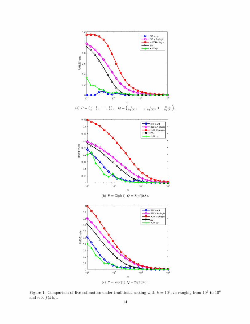
where f(k) = 5. For this pair of (P,Q), the density ratio is f(k) for all but one of the bins, which is ina sense a worst-case for the KL divergence estimation problem. We let m range from 103 to 106 and setn = 3f(k)m. The second type is given by (P,Q) = (Zipf(1),Zipf(0.8)) and (P,Q) = (Zipf(1),Zipf(0.6)). TheZipf distribution is a discrete distribution that is commonly used in linguistics, insurance, and the modeling

of rare events. If P = Zipf(α), then Pi = i−α∑kj=1 j

−α , for 1 ≤ i ≤ k. We let m range from 103 to 106 and set

n = 0.5f(k)m, where f(k) is computed for these two pairs of Zipf distributions, respectively.

In Fig. 1, we plot the root mean square errors (RMSE) of the five estimators as a function of the samplesize m for these three pairs of distributions. It is clear from the figure that our minimax optimal estimator(BZLV opt) and the HJW minimax optimal estimator (HJW opt) outperform the other three approaches.Such a performance improvement is significant especially when the sample size is small. Furthermore, ouraugmented plug-in estimator (BZLV A-plugin) has a much better performance than the HJW modified

12

plug-in estimator (HJW M-plugin), because the bias of estimating∑ki=1 Pi logPi and the bias of estimating∑k

i=1 Pi logQi may cancel each other out by the design of our augmented plug-in estimator. Furthermore,the RMSEs of all the five estimators converge to zero when the number of samples are sufficiently large.

We next compare the performance of the five estimators under the large-alphabet setting, in which we let

k range from 103 to 106, and set m = 2klog k and n = kf(k)

log k . We use the same three pairs of distributions as inthe previous setting. In Fig. 2, we plot the RMSEs of the five estimators as a function of k. It is clear fromthe figure that our minimax optimal estimator (BZLV opt) and the HJW minimax optimal estimator (HJWopt) have very small estimation errors, which is consistent with our theoretical results of the minimax riskbound. However, the RMSEs of the other three approaches increase with k, which implies that m = 2k

log k ,

n = kf(k)log k are insufficient for those estimators.

6 Conclusion

In this paper, we studied the estimation of KL divergence between large-alphabet distributions. Weshowed that there exists no consistent estimator for KL divergence under the worst-case quadratic risk overall distribution pairs. We then studied a more practical set of distribution pairs with bounded density ratio.We proposed an augmented plug-in estimator, and characterized tight sufficient and necessary conditionson the sample complexity for such an estimator to be consistent. We further designed a minimax optimalestimator by employing a polynomial approximation along with the plug-in approach, and established theoptimal minimax rate. We anticipate that the designed KL divergence estimator can be used in variousapplication contexts including classification, anomaly detection, community clustering, and nonparametrichypothesis testing.

13

(a) P =(1k, 1

k, · · · , 1

k

), Q =

(1

kf(k), · · · , 1

kf(k), 1 − k−1

kf(k)

).

(b) P = Zipf(1), Q = Zipf(0.8).

(c) P = Zipf(1), Q = Zipf(0.6).

Figure 1: Comparison of five estimators under traditional setting with k = 104, m ranging from 103 to 106

and n � f(k)m.14

(a) P =(1k, 1

k, · · · , 1

k

), Q =

(1

kf(k), · · · , 1

kf(k), 1 − k−1

kf(k)

).

(b) P = Zipf(1), Q = Zipf(0.8).

(c) P = Zipf(1), Q = Zipf(0.6).

Figure 2: Comparison of five estimators under large-alphabet setting with k ranging from 103 to 106,

m = 2klog k and n = kf(k)

log k .15

A Proof of Theorem 1

For any fixed (k,m, n), applying Le Cam’s two-point method, we have

R∗(k,m, n) ≥ 1

16(D(P (1)‖Q(1))−D(P (2)‖Q(2)))2 exp

(−mD(P (1)‖P (2))− nD(Q(1)‖Q(2))

). (46)

The idea here is to keep P (1) close to P (2), and Q(1) close to Q(2), so that D(P (1)‖P (2)) ≤ 1m , D(Q(1)‖Q(2)) ≤

1n , but keep (D(P (1)‖Q(1))−D(P (2)‖Q(2)))2 large. We construct the following two pairs of distributions:

P (1) = P (2) =

(1

2(k − 1), . . . ,

1

2(k − 1),

1

2

), (47)

Q(1) =

(1− ε1k − 1

, . . . ,1− ε1k − 1

, ε1

), (48)

Q(2) =

(1− ε2k − 1

, . . . ,1− ε2k − 1

, ε2

), (49)

where 0 < ε1 < 1/4, and ε2 = ε1 + 14n <

12 . By such a construction, we obtain,

D(P (1)‖P (2)) = 0, (50)

D(Q(1)‖Q(2)) = (1− ε1) log1− ε11− ε2

+ ε1 logε1ε2. (51)

Furthermore,

D(Q(1)‖Q(2)) = (1− ε1) log

(1 +

ε2 − ε11− ε2

)+ ε1 log

ε1

ε1 + 14n

= (1− ε1) log

(1 +

1

4n(1− ε2)

)+ ε1 log

ε1

ε1 + 14n

<1− ε1

4n(1− ε2). (52)

Since ε1 > 0 and ε2 < 1/2, we obtain D(Q(1)‖Q(2)) ≤ 12n .

By the construction of (P (1), Q(1)) and (P (2), Q(2)),

(D(P (1)‖Q(1))−D(P (2)‖Q(2))

)2=

(1

2log(1− ε2

1− ε1)

+1

2log

ε2ε1

)2

=

(1

2log(1− ε2

1− ε1)

+1

2log(1 +

1

4nε1

))2

. (53)

Note that | 12 log(

1−ε21−ε1

)| is upper bounded by log 2. The only constraint for (53) is 0 < ε1 < 1/4. Hence,

we can choose ε1 to be arbitrarily small, such that 14nε1

is arbitrarily large for any fixed k, m and n.Consequently,

(D(P (1)‖Q(1))−D(P (2)‖Q(2))

)2=

(1

2log(1− ε2

1− ε1)

+1

2log(1 +

1

4nε1

))2

→∞, as ε1 → 0. (54)

Therefore, the minimax quadratic risk lower bound is infinity for any fixed k, m and n, which implies thatthere does not exist any consistent estimator over the set Mk.

16

B Proof of Proposition 1

The quadratic risk can be decomposed into the square of the bias and the variance as follows:

E[(DA−plug−in(M,N)−D(P‖Q))2

]=

(E[DA−plug−in(M,N)−D(P‖Q)

])2

+ Var[DA−plug−in(M,N)

].

We bound the bias and the variance in the following two subsections, respectively.

B.1 Bounding the Bias

The bias of the augmented plug-in estimator can be written as,∣∣∣E(DA−plug−in(M,N)−D(P‖Q))∣∣∣

=

∣∣∣∣∣E(

k∑i=1

[Mi

mlog

Mi/m

(Ni + 1)/n− Pi log

PiQi

])∣∣∣∣∣=

∣∣∣∣∣E(

k∑i=1

[Mi

mlog

Mi

m− Pi logPi

])+ E

(k∑i=1

[Pi logQi −

Mi

mlog

Ni + 1

n

])∣∣∣∣∣=

∣∣∣∣∣E(

k∑i=1

[Mi

mlog

Mi

m− Pi logPi

])+ E

(k∑i=1

Pi lognQiNi + 1

)∣∣∣∣∣≤

∣∣∣∣∣E(

k∑i=1

[Mi

mlog

Mi

m− Pi logPi

])∣∣∣∣∣+

∣∣∣∣∣E(

k∑i=1

Pi lognQiNi + 1

)∣∣∣∣∣ . (55)

The first term in (55) is the bias of the plug-in estimator for entropy estimation, which can be bounded asin [23]: ∣∣∣∣∣E

(k∑i=1

[Mi

mlog

Mi

m− Pi logPi

])∣∣∣∣∣ ≤ log

(1 +

k − 1

m

)<

k

m. (56)

Next, we bound the second term in (55) as follows:

E

(k∑i=1

Pi lognQiNi + 1

)=−

k∑i=1

PiE(

log(1 +

Ni + 1− nQinQi

))(a)

≥ −k∑i=1

PiE(Ni + 1− nQi

nQi

)

=−k∑i=1

Pi1

nQi

≥− kf(k)

n, (57)

where (a) is due to the fact that log(1 + x) ≤ x. Furthermore, by Jensen’s inequality, we have,

E

(k∑i=1

Pi lognQiNi + 1

)=

k∑i=1

PiE(

lognQiNi + 1

)≤

k∑i=1

Pi logE[nQiNi + 1

]. (58)

Let B(n, p) denote the Binomial distribution where n is the total number of experiments, and p is theprobability that each experiment yields a desired outcome. Note that since Ni ∼ B(n,Qi), and then the

17

expectation in (58) can be computed as follows:

E[

1

Ni + 1

]=

n∑j=0

1

j + 1

(n

j

)Qji (1−Qi)

n−j

=

n∑j=0

1

j + 1

n!

(n− j)!j!Qji (1−Qi)

n−j

=1

n+ 1

n∑j=0

(n+ 1)!

(n− j)!(j + 1)!Qji (1−Qi)

n−j

=1

(n+ 1)Qi

n∑j=0

(n+ 1

j + 1

)Qj+1i (1−Qi)n−j

=1

(n+ 1)Qi(1− (1−Qi)n+1) <

1

nQi. (59)

Thus, we obtain

E

(k∑i=1

Pi lognQiNi + 1

)≤

k∑i=1

Pi logE[nQiNi + 1

]<

k∑i=1

Pi lognQinQi

= 0. (60)

Combining (57) and (60), we obtain the following upper bound for the second term in the bias,∣∣∣∣∣E(

k∑i=1

Pi lognQiNi + 1

)∣∣∣∣∣ ≤ kf(k)

n. (61)

Hence, ∣∣∣∣E(DA−plug−in(M,N)−D(P‖Q)

)∣∣∣∣ < k

m+kf(k)

n. (62)

B.2 Bounding the Variance

Applying the Efron-Stein Inequality [24, Theorem 3.1], we have:

Var[DA−plug−in(M,N)]

≤ m

2E[(DA−plug−in(M,N)− DA−plug−in(M ′, N))2

]+n

2E[(DA−plug−in(M,N)− DA−plug−in(M,N ′))2

],

(63)

where M ′ and N ′ are the histograms of (X1, . . . , Xm−1, X′m) and (Y1, . . . , Yn−1, Y

′n), respectively. Here, X ′m

is an independent copy of Xm and Y ′n is an independent copy of Yn.

Let M = (M1, . . . , Mk) be the histogram of (X1, . . . , Xm−1), N = (N1, . . . , Nk) be the histogram of(Y1, . . . , Yn−1). Then M ∼ Multinomial(m−1, P ) is independent fromXm andX ′m, and N ∼ Multinomial(n−1, Q) is independent from Yn and Y ′n. Denote the function φ as

φ(x, y) , x log x− x log y. (64)

Using this notation, the augmented plug-in estimator can be written as

DA−plug−in(M,N) =

k∑i=1

φ(Mi

m,Ni + 1

n). (65)

18

Let MXm be the number of samples in bin Xm. We can bound the first term in (63) as follows:

E[(DA−plug−in(M,N)− DA−plug−in(M ′, N))2

]=E

[E

[(φ(MXm + 1

m,NXm + 1

n

)+ φ

(MX′m

m,NX′m + 1

n

)− φ

(MXm

m,NXm + 1

n

)− φ

(MX′m+ 1

m,NX′m + 1

n

))2∣∣∣∣Xm, X′m

]](a)

≤4E

[E

[(φ(MXm + 1

m,NXm + 1

n

)− φ

(MXm

m,NXm + 1

n

))2∣∣∣∣Xm

]]

=4

k∑j=1

E

[(φ(Mj + 1

m,Nj + 1

n

)− φ

(Mj

m,Nj + 1

n

))2]Pj

=4

m2

k∑j=1

E

[((Mj + 1) log

Mj + 1

m− Mj log

Mj

m− log

Nj + 1

n

)2]Pj

=4

m2

k∑j=1

E

[(log

Mj + 1

m+ Mj log(1 +

1

Mj

)− logNj + 1

n

)2]Pj

(b)

≤ 8

m2+

8

m2

k∑j=1

E

[(log

Mj + 1

m− log

Nj + 1

n

)2]Pj . (66)

where (a) is due to the fact that Xm is independent and identically distributed as X ′m, and (b) is due to thefact that 0 ≤ x log(1 + 1

x ) ≤ 1 for all x > 0. We rewrite the second term in (66) as follows,

E

[(log

Mj + 1

m

n

Nj + 1

)2]

=E

[(log

Mj + 1

m

n

Nj + 11{Mj≤

mPj2 }

1{Nj>

nQj2 }

)2]

+ E

[(log

Mj + 1

m

n

Nj + 11{Mj>

mPj2 }

1{Nj>

nQj2 }

)2]

+ E

[(log

Mj + 1

m

n

Nj + 11{Mj≤

mPj2 }

1{Nj≤

nQj2 }

)2]

+ E

[(log

Mj + 1

m

n

Nj + 11{Mj>

mPj2 }

1{Nj≤

nQj2 }

)2].

To analyze the above equation, we first observe the following properties that are useful:

If Mj ≤mPj

2, then

1

m≤ Mj + 1

m≤ Pj

2+

1

m;

If Mj >mPj

2, then

Pj2

+1

m<Mj + 1

m≤ 1;

If Nj >nQj

2, then

Qj2

+1

n<Nj + 1

n≤ 1 +

1

n;

If Nj ≤nQj

2, then

1

n≤ Nj + 1

n≤ Qj

2+

1

n.

With the above bounds, and assuming that m > 2, n > 2, we next analyze the following four cases.

19

1. If Mj ≤ mPj2 and Nj >

nQj2 , then we have n

m(n+1) ≤Mj+1m

nNj+1 ≤

Pj2 + 1

mQj2 + 1

n

, and

E

[(log

Mj + 1

m

n

Nj + 11{Mj≤m2 Pj}

1{Nj>

nQj2 }

)2]

≤

[log2(

n

m(n+ 1)) +

(log(

Pj2

+1

m)− log(

Qj2

+1

n)

)2]P(Mj ≤

m

2Pj

)(c)

≤

[log2(

1

2m) +

(log(

Pj2

+1

m)− log(

Qj2

+1

n)

)2]

exp(− (m− 2)Pj

8

)≤2

[log2(

1

2m) +

(log2(

Pj2

+1

m) + log2(

Qj2

+1

n)

)]exp

(− (m− 2)Pj

8

)≤2

[log2(2m) +

(log2(

Pj2

) + log2(Qj2

)

)]exp

(− (m− 2)Pj

8

). (67)

where (c) follows from the Chernoff bound on the binomial tail.

2. If Mj >mPj

2 and Nj >nQj

2 , then we have nn+1 (

Pj2 + 1

m ) ≤ Mj+1m

nNj+1 ≤

1Qj2 + 1

n

, and

E

[(log

Mj + 1

m

n

Nj + 11{Mj>

m2 Pj}

1{Nj>

nQj2 }

)2]

≤[log2(

n

n+ 1(Pj2

+1

m)) + log2(

Qj2

+1

n)

]≤2

[log2(

Pj4

) + log2(Qj2

)

]. (68)

3. If Mj ≤ mPj2 and Nj ≤ nQj

2 , then we have 1

m(Qj2 + 1

n )≤ Mj+1

mn

Nj+1 ≤nPj

2 + nm , and

E

[(log

Mj + 1

m

n

Nj + 11{Mj≤m2 Pj}

1{Nj≤

nQj2 }

)2]

≤[log2(m(

Qj2

+1

n)) + log2(n(

Pj2

+1

m))

]exp

(− (m− 2)Pj

8

)exp

(− nQj

8

)≤2

[(log2(

Qj2

) + log2m) + (log2(Pj2

) + log2 n)

]exp

(− (m− 2)Pj

8

)exp

(− nQj

8

). (69)

4. If Mj >mPj

2 and Nj ≤ nQj2 , then we have

Pj2 + 1

mQj2 + 1

n

≤ Mj+1m

nNj+1 ≤ n, and

E

[(log

Mj + 1

m

n

Nj + 11{Mj>

m2 Pj}

1{Nj≤

nQj2 }

)2]

≤

[(log(

Pj2

+1

m)− log(

Qj2

+1

n)

)2

+ log2 n

]exp

(− nQj

8

)≤2

[log2 n+

(log2(

Pj2

) + log2(Qj2

)

)]exp

(− nQj

8

). (70)

20

Combining the four cases together, we have


]≤ 8

m2+

8

m2

k∑j=1

E

[(log

Mj + 1

m− log

Nj + 1

n

)2]Pj

≤ 16

m2

k∑j=1

Pj

[(log2(

Qj2

) + log2m) + (log2(Pj2

) + log2 n)

]exp

(− (m− 2)Pj

8

)exp

(− nQj

8

)+

16

m2

k∑j=1

Pj

[log2(2m) +

(log2(

Pj2

) + log2(Qj2

)

)]exp

(− (m− 2)Pj

8

)+

16

m2

k∑j=1

Pj

[log2(n) +

(log2(

Pj2

) + log2(Qj2

)

)]exp

(− nQj

8

)+

16

m2

k∑j=1

Pj

[log2(

Pj4

) + log2(Qj2

)

]+

8

m2

≤ 16

m2

k∑j=1

Pj

[4 log2(

4

Pj) + 4 log2(

2

Qj) + 2 log2(2m) exp

(− (m− 2)Pj

8

)+ 2 log2 n exp

(− nQj

8

)]+

8

m2.

(71)

Now, we analyze the asymptotic behavior of the above four terms in (71):

1. It can be shown that∑kj=1−Pj logPj ≤ log k and

∑kj=1 Pj log2 Pj ≤ log2 k. Hence, we obtain

k∑j=1

Pj log2(4

Pj) =

k∑j=1

Pj(log2(Pj) + log2 4− 2 logPj log 4) ≤ (log k + log 4)2. (72)

2. Given the bounded ratio constraint 1Qj≤ f(k)

Pj, we have

k∑j=1

Pi log2(2

Qj) ≤

k∑j=1

Pj log2 2f(k)

Pj=

k∑j=1

Pi(log2 2f(k)+log2 Pj−2 log 2f(k) logPj) ≤ (log k+log 2f(k))2.

(73)

3. Since supx>0 x exp(−nx/8) = 8ne , we have

k∑i=1

Pi log2(2m) exp(− (m− 2)Pj

8

)≤

k∑i=1

8 log2(2m)

(m− 2)e≤ 8k log2(2m)

(m− 2)e. (74)

4. Since Qj ≥ Pjf(k) , and supx>0 x exp(−nx/8) = 8

ne , we have

k∑i=1

Pi log2 n exp(− nQj

8

)≤

k∑i=1

log2 nPi exp(− nPj

8f(k)

)≤ 8kf(k) log2 n

ne. (75)

Thus,


].

(log f(k) + log k)2

m2+k log2m

m3+kf(k) log2 n

m2n

.(log f(k) + log k)2

m2

(1 +

k log2m

m log2 k+

kf(k) log2 n

log2(kf(k))n

), (76)

21

where the second term applies kf(k) ≥ k. Note that the assumption m & k and n & kf(k) implies thatk log2mm log2 k

. 1 and kf(k) log2 nlog2(kf(k))n

. 1, because xlog x is an increasing function. We then obtain,


].

log2 f(k) + log2 k

m2. (77)

The second term in (63) can be bounded similarly as follows:

E[(DA−plug−in(M,N)− DA−plug−in(M,N ′))2

]=E

[E

[(φ(MYm

m,NYm + 2

n

)+ φ

(MY ′m

m,NY ′m + 1

n

)− φ

(MYm

m,NYm + 1

n

)− φ

(MY ′m

m,NY ′m + 2

n

))2∣∣∣∣Ym, Y ′m]]

≤4E

[E

[(φ(MYm

m,NYm + 2

n

)− φ

(MYm

m,NYm + 1

n

))2∣∣∣∣Ym]]

=4

k∑j=1

E

[(φ(Mj

m,Nj + 2

n

)− φ

(Mj

m,Nj + 1

n

))2]Qj

=4

k∑j=1

E

[(Mj

mlog(

1 +1

Nj + 1

))2]Qj

=4

m2

k∑j=1

E[M2j

]E

[log2

(1 +

1

Nj + 1

)]Qj . (78)

Since Mj follows the binomial distribution, we compute E [Mj ]2

as follows:

E[M2j

]= E[Mj ]

2 + Var(Mj) = m2P 2j +mPj(1− Pj). (79)

We can also derive,

E

[log2

(1 +

1

Nj + 1

)]≤ E

[( 1

Nj + 1

)2]≤ E

[2

(Nj + 1)(Nj + 2)

]≤ 2

(n− 1)2Q2j

, (80)

where the last inequality follows similarly from (59). Thus,

E[(DA−plug−in(M,N)− DA−plug−in(M,N ′))2

]=

4

m2

k∑j=1

E[M2j

]E

[log2

(1 +

1

Nj + 1

)]Qj

≤4

k∑j=1

(P 2j +

Pj(1− Pj)m

)2

(n− 1)2Q2j

Qj

.k∑j=1

PjQj

(Pj +

1

m

)2

n2

.f(k)

n2+kf(k)

n2m. (81)

Combing (77) and (81), we obtain the following upper bound on the variance:

Var[DA−plug−in(M,N)]

≤m2E[(DA−plug−in(M,N)− DA−plug−in(M ′, N))2

]+n

2E[(DA−plug−in(M,N)− DA−plug−in(M,N ′))2

].

log2 k

m+

log2 f(k)

m+f(k)

n+kf(k)

nm. (82)

22

Note that the term kf(k)nm in the variance can be further upper bounded as follows

kf(k)

nm≤ kf(k)

n

k

m≤(kf(k)

n+k

m

)2

. (83)

Combining (62), (82) and (83), we obtain the following upper bound on the worse case quadratic risk foraugmented plug-in estimator:

R(DA−plug−in, k,m, n, f(k)) .

(kf(k)

n+k

m

)2

+log2 k

m+

log2 f(k)

m+f(k)

n. (84)

C Proof of Proposition 2

In this section, we derive necessary conditions on the sample complexity to guarantee consistency of theaugmented plug-in estimator over Mk,f(k). We first show that m� k and n� kf(k) is necessary by lower

bounding the squared bias. We then show that m� log2 f(k) is necessary by Le Cam’s two-point method.

C.1 m� k and n� kf(k) are Necessary

It can be shown that the mean square error is lower bounded by the squared bias, which is as follows:

E[(DA−plug−in(M,N)−D(P‖Q)

)2] ≥ (E [DA−plug−in(M,N)−D(P‖Q)])2

. (85)

Following steps in (55), we have:

E[DA−plug−in(M,N)−D(P‖Q)] = E

(k∑i=1

(Mi

mlog

Mi

m− Pi logPi

))+ E

(k∑i=1

Pi lognQiNi + 1

). (86)

The first term in (86) is the bias of plug-in entropy estimator. As shown in [14] and [23], the worst casequadratic risk of the first term can be bounded as follows:

E

(k∑i=1

(Mi

mlog

Mi

m− Pi logPi

))≥ (

k

m∧ 1), if P is uniform distribution, (87a)

E

(k∑i=1

(Mi

mlog

Mi

m− Pi logPi

))≤ log

(1 +

k − 1

m

), for any P . (87b)

As shown in (57), we have the following bound on the second term in (86):

−kf(k)

n≤ E

(k∑i=1

Pi lognQiNi + 1

), for any (P,Q). (88)

In order to obtain a tight bound for the bias, we choose the following (P,Q):

P =

(1

k,

1

k, · · · , 1

k

), Q =

(1

kf(k), · · · , 1

kf(k), 1− k − 1

kf(k)

). (89)

23

It can be verified that P and Q satisfy the density ratio constraint. For this a (P,Q) pair, we have

E

(k∑i=1

Pi lognQiNi + 1

)≤

k∑i=1

Pi logE[nQiNi + 1

]

=

k∑i=1

Pi log

(nQi

(n+ 1)Qi(1− (1−Qi)n+1)

)

≤k∑i=1

Pi log(1− (1−Qi)n+1)

≤ k − 1

klog(1− (1− 1

kf(k))n+1)

≤ −k − 1

k(1− 1

kf(k))n+1

= −k − 1

k(1− 1

kf(k))kf(k)(n+1) 1

kf(k) . (90)

Since (1− x)1/x is decreasing on [0, 1], and limx→0(1− x)1/x = 1e , for sufficiently large k, 1/(kf(k)) is close

to 0 , and thus we have,

e−1 > (1− 1

kf(k))kf(k) > e−β0 , (91)

where β0 > 1 is a constant. Thus,

E

(k∑i=1

Pi lognQiNi + 1

)≤ −k − 1

kexp(− β0n

kf(k)), for (P,Q) in (89). (92)

Combining (87a) and (57), we have

(k

m∧ 1)− kf(k)

n≤ sup

(P,Q)∈Mk,f(k)

E[DA−plug−in(M,N)−D(P‖Q)], (93)

and combining (87b) and (92), we obtain

E[DA−plug−in(M,N)−D(P‖Q)] ≤ log

(1 +

k

m

)− k − 1

kexp(− β0n

kf(k)), for (P,Q) in (89). (94)

1) If m . k and n� kf(k), let m ≤ C1k, where C1 is a positive constant. Then (93) suggests

sup(P,Q)∈Mk,f(k)

E[DA−plug−in(M,N)−D(P‖Q)] ≥ (k

m∧ 1)− kf(k)

n→ (

1

C1∧ 1). (95)

The bias is lower bounded by a positive constant, and hence, for sufficiently large k, the augmentedplug-in estimator is not consistent.

2) If m� k and n . kf(k), let n ≤ C2kf(k), where C2 is a positive constant. Then (94) suggests


(1 +

k

m

)− k − 1

kexp (− β0n

kf(k))

→ −k − 1

kexp (− β0n

kf(k))

≤ −k − 1

ke−β0C2 . (96)

The bias is upper bounded by a negative constant, and hence, for sufficiently large k, the augmentedplug-in estimator is not consistent.

24

3) If m . k and n . kf(k), we cannot get a useful lower bound on the squared bias from (93) and (94)using the chosen pair (P,Q). Hence, we need to choose other pairs (P,Q).

The bias of the augmented plug-in estimator can be decomposed into: 1) bias due to estimating∑ki=1 Pi logPi;

and 2) bias due to estimating∑ki=1 Pi logQi. It can be shown that the first bias term is always positive,

because x log x is a convex function. The second bias term is always negative for any distribution Q. Hence,the two bias terms may cancel out partially or even fully. Thus, to show that the risk is bounded away fromzero, we first determine which bias term dominates, and then construct a pair of distributions such that thedominant bias term is either lower bounded by a positive constant or upper bounded by a negative constant.

Case I: If km ≥ (1 + ε)αkf(k)

n , where ε > 0 and 0 < α < 1 are constants, and which implies that thenumber of samples drawn from P is relatively smaller than the number of samples drawn from Q, the firstbias term dominates. We then set:

P =

(1

k,

1

k, · · · , 1

k

), Q =

(1

αkf(k), · · · , 1

αkf(k), 1− k − 1

αkf(k)

). (97)

Let α > 1f(k) , and then 1− k−1

αkf(k) >1k . It can be verified that the density ratio between P and Q is bounded

by αf(k) ≤ f(k). Since P is a uniform distribution, which has the maximal entropy, the bias of entropyestimation can be written as

E

(k∑i=1

(Mi

mlog

Mi

m− Pi logPi

))= log k + E

(k∑i=1

Mi

mlog

Mi

m

). (98)

It can be shown that,k∑i=1

Mi

mlog

Mi

m≥ − logm. (99)

Combining with (87a) and (87b), we have

(k

m∧ 1) ∨ log

k

m≤ E

(k∑i=1

(Mi

mlog

Mi

m− Pi logPi

))≤ log

(1 +

k

m

). (100)

And for the above choice of (P,Q),

E

(k∑i=1

(Pi logQi −

Mi

mlog

Ni + 1

n

))= −

k∑i=1

PiE[log

Ni + 1

nQi

]

≥ −k∑i=1

Pi logE[Ni + 1

nQi

]

= −k∑i=1

Pi log

(1 +

1

nQi

)≥ −k − 1

klog

(1 +

αkf(k)

n

)− 1

klog

(1 +

k

n

)≥ − log

(1 +

αkf(k)

n

)− log 2k

k. (101)

Combining with (100), we obtain the following lower bound,

E[DA−plug−in(M,N)−D(P‖Q)] ≥ (k

m∧ 1) ∨ log

k

m− log

(1 +

αkf(k)

n

)− log 2k

k

≥ (k

m∧ 1) ∨ log

k

m− log

(1 +

k

m(1 + ε)

)− log 2k

k. (102)

25

Note that m . k. Let m ≤ C1k, where C1 is a positive constant. Without loss of generality, we can assumethat C1 > 1, since the case C1 ≤ 1 is included in the following discussion.

Denote x = km , x ∈ [ 1

C1,∞]. If x ∈ [ 1

C1, 1], then (x ∧ 1) ∨ log x = x, and it can be shown that

x− log

(1 +

x

1 + ε

)≥ x− x

1 + ε≥ ε

C1(1 + ε). (103)

If x ∈ (1, e], then (x ∧ 1) ∨ log x = 1, and it can be shown that

1− log

(1 +

x

1 + ε

)≥ 1− log

(1 +

e

1 + ε

). (104)

If x ∈ (e,∞), then (x ∧ 1) ∨ log x = log x, it can be shown that

log x− log

(1 +

x

1 + ε

)= log

(1

1x + 1

1+ε

)≥ 1− log

(1 +

e

1 + ε

). (105)

Combining (103), (104) and (105), we obtain

(x ∧ 1) ∨ log x− log

(1 +

x

1 + ε

)≥ min

(ε

C1(1 + ε), 1− log

(1 +

e

1 + ε

)). (106)

If ε > 1e−1 , the right hand side in the above inequality is positive. And for sufficiently large k, log(2k)

kis arbitrarily small. This implies that the worst case quadratic error is also lower bounded by a positiveconstant, and hence, the augmented plug-in estimator is not consistent.

Case II: If km < (1 + ε)αkf(k)

n , which implies that the number of samples drawn from P is relatively largerthan the number of samples drawn from Q, then the second bias term dominates.

Since n . kf(k), assume that n ≤ C2kf(k), where C2 is a positive constant. Without loss of generality,we assume that C2 > 1.

For n ≤ kf(k), we set:

P =

(1

k,

1

k, · · · , 1

k

), Q =

(1

kf(k), · · · , 1

kf(k), 1− k − 1

kf(k)

). (107)

Following the steps in (90) and (91), we have


(1 +

k

m

)+k − 1

klog(1− exp(− β0n

kf(k)))

=k − 1

k

(log

(1 +

k

m

)+ log(1− exp(− β0n

kf(k)))

)+

1

klog

(1 +

k

m

)≤k − 1

klog

((1 + (1 + ε)

αkf(k)

n

)(1− exp(− β0n

kf(k))))

+log(2k)

k. (108)

Let β , (1 + ε)α, and t = nkf(k) . Then, we define the function

h(t) , (1 +β

t)(1− exp(−β0t)), t ∈ (0, 1). (109)

For sufficiently large k, we choose β0 = 1.05. Then for any β < 0.3, we have

h(t) = (1 +β

t)(1− exp(−1.05t)) < 0.9, ∀t ∈ (0, 1). (110)

26

Thus, if f(k) is large, e.g., f(k) > 6, then we can find α that satisfies the condition α > 1f(k) and (1+ε)α < 0.3,

with ε > 1e−1 . Then, for sufficiently large k,

E[DA−plug−in(M,N)−D(P‖Q)] ≤ k − 1

klog

((1 + (1 + ε)

αkf(k)

n

)(1− exp(− β0n

kf(k))))

+log(2k)

k

→ log

((1 + (1 + ε)

αkf(k)

n

)(1− exp(− 1.05n

kf(k))))

≤ log 0.9 < 0. (111)

For kf(k) < n ≤ C2kf(k), we set:

P =

(f(k)

n, . . . ,

f(k)

n, 1− (k − 1)f(k)

n

), Q =

(1

n, . . . ,

1

n, 1− k − 1

n

). (112)

It can be shown that (P,Q) satisfy the density ratio constraint. Following the steps for deriving (90), wehave


(1 +

k

m

)+

(k − 1)f(k)

nlog(1− (1− 1

n)n+1)

(a)

≤ k

m− 0.3

(k − 1)f(k)

n

≤ (1 + ε)αkf(k)

n− 0.3

kf(k)

n+

0.3f(k)

n

= ((1 + ε)α− 0.3)kf(k)

n+

0.3f(k)

n(b)

≤ ((1 + ε)α− 0.3)1

C2+

0.3

k(c)< 0 (113)

where (a) is due to the fact that log(1− (1− 1n )n+1) ≤ −0.3 for n ≥ 5; (b) holds if (1 + ε)α − 0.3 < 0; and

(c) holds for sufficiently large k.

This implies that for large k,

E[DA−plug−in(M,N)−D(P‖Q)] < c < 0, (114)

where c is a negative constant. Hence, the worse case quadratic risk is lower bounded by a positive constant,and the augmented plug-in estimator is not consistent in this case.

C.2 m� log2 f(k) is Necessary

It suffices to show that the augmented plug-in estimator is not consistent when m . log2 f(k). We use theminimax risk as the lower bound of the worst case quadratic risk for augmented plug-in estimator. To thisend, we apply Le Cam’s two-point method. We first construct two pairs of distributions as follows:

P (1) =

(1

3(k − 1), . . . ,

1

3(k − 1),

2

3

), (115)

P (2) =

(1− ε

3(k − 1), . . . ,

1− ε3(k − 1)

, 1− 1− ε3

), (116)

Q(1) = Q(2) =

(1

3(k − 1)f(k), . . . ,

1

3(k − 1)f(k), 1− 1

3f(k)

). (117)

27

The above distributions satisfy:

D(P (1)‖Q(1)) =1

3log f(k) +

2

3log

23

1− 13f(k)

, (118)

D(P (2)‖Q(2)) =1− ε

3log(1− ε)f(k) +

(1− 1− ε

3

)log

1− 1−ε3

1− 13f(k)

, (119)

D(P (1)‖P (2)) =1

3log

1

1− ε+

2

3log

23

1− 1−ε3

. (120)

We set ε = 1√m

, and then obtain

D(P (1)‖P (2)) =1

3log

(1 +

ε

1− ε

)+

2

3log

(1− ε

2 + ε

)≤ ε

3(1− ε)− 2

3

ε

2 + ε

=ε2

(1− ε)(2 + ε)≤ 1

m. (121)

Furthermore,

D(P (1)‖Q(1))−D(P (2)‖Q(2))

=1

3log f(k) +

2

3log

23

1− 13f(k)

− 1− ε3

log(1− ε)f(k)−(

1− 1− ε3

)log

1− 1−ε3

1− 13f(k)

=1

3log

1

1− ε+ε

3log(1− ε)f(k) +

2

3log

2

2 + ε− ε

3log

2 + ε

3− 1f(k)

=1

3log

1

1− ε4

(2 + ε)2− ε

3log

2 + ε

(1− ε)(3f(k)− 1), (122)

which implies that

(D(P (1)‖Q(1))−D(P (2)‖Q(2)))2 & ε2 log2 2

(3f(k)− 1)� log2 f(k)

m, (123)

as m→∞. Now applying Le Cam’s two-point method, we obtain

R∗(k,m, n, f(k)) ≥ 1

16(D(P (1)‖Q(1))−D(P (2)‖Q(2)))2 exp

(−mD(P (1)‖P (2))− nD(Q(1)‖Q(2))

). (124)

Clearly, if m . log2 f(k), the minimax quadratic risk does not converge to 0 as k →∞, which further impliesthat the augmented plug-in estimator is not consistent for this case.

D Proof of Lemma 1

We prove the inequality (21) that connects the minimax risk (8) under the deterministic sample size tothe risk (20) under the Poisson sampling model. We first prove the left hand side of (21). Recall that

28

0 ≤ R∗(k,m, n, f(k)) ≤ log2 f(k) and R∗(k,m, n, f(k)) is decreasing with m,n. Therefore,

R∗(k, 2m, 2n, f(k)) =∑i≥0

∑j≥0

R∗(k, i, j, f(k))Poi(2m, i)Poi(2n, i)

=∑

i≥m+1

∑j≥n+1

R∗(k, i, j, f(k))Poi(2m, i)Poi(2n, i) +∑i≥0

n∑j=0


+

m∑i=0

∑j≥n+1


≤ R∗(k,m, n, f(k)) + e−(1−log 2)n log2 f(k) + e−(1−log 2)m log2 f(k), (125)

where the last inequality follows from the Chernoff bound P[Poi(2n) ≤ n] ≤ exp(−(1 − log 2)n). We thenprove the right hand side of (21). By the minimax theorem,

R∗(k,m, n, f(k)) = supπ

infD

E[(D(M,N)−D(P‖Q))2], (126)

where π ranges over all probability distribution pairs on Mk,f(k) and the expectation is over (P,Q) ∼ π.

Fix a prior π and an arbitrary sequence of estimators {Dm,n} indexed by the sample sizes m and n. It

is unclear whether the sequence of Bayesian risks αm,n = E[(Dm,n(M,N)−D(P‖Q))2] with respect to π isdecreasing in m or n. However, we can define {αi,j} as

α0,0 = α0,0, αi,j = αi,j ∧ αi−1,j ∧ αi,j−1. (127)

Further define,

Dm,n(M,N) ,

Dm,n(M,N), if αm,n = αm,n;

Dm−1,n(M,N), if αm,n = αm−1,n;

Dm,n−1(M,N), if αm,n = αm,n−1.

(128)

Then for m′ ∼ Poi(m/2) and n′ ∼ Poi(n/2), and (P,Q) ∼ π, we have

E[(Dm′,n′(M

′, N ′)−D(P‖Q))2]

=∑i≥0

∑j≥0

E[(Di,j(M

′, N ′)−D(P‖Q))2]

Poi(m

2, i)Poi(

n

2, j)

≥∑i≥0

∑j≥0

E[(Di,j(M,N)−D(P‖Q))2

]Poi(

m

2, i)Poi(

n

2, j)

≥m∑i=0

n∑j=0

E[(Di,j(M,N)−D(P‖Q))2

]Poi(

m

2, i)Poi(

n

2, j)

(a)

≥ 1

4E[(Dm,n(M,N)−D(P‖Q))2

], (129)

where (a) is due to the Markov’s inequality: P[Poi(n/2) ≥ n] ≤ 12 . If we take infimum of the left hand side

over Dm,n, then take supremum of both sides over π, and use the Bayesian risk as a lower bound on theminimax risk, then we can show that

R∗(k,m

2,n

2, f(k)) ≥ 1

4R∗(k,m, n, f(k)). (130)

29

E Proof of Proposition 3

E.1 Bounds Using Le Cam’s Two-Point Method

E.1.1 Proof of R∗(k,m, n, f(k)) & log2 f(k)m

Following the same steps in Appendix C.2, we can show

R∗(k,m, n, f(k)) & (D(P (1)‖Q(1))−D(P (2)‖Q(2)))2 &log2 f(k)

m. (131)

E.1.2 Proof of R∗(k,m, n, f(k)) & f(k)n

We construct two pairs of distributions as follows:

P (1) = P (2) =

(1

3(k − 1), 0,

1

3(k − 1), 0, . . . ,

5

6

), (132)

Q(1) =

(1

2(k − 1)f(k), . . . ,

1

2(k − 1)f(k), 1− 1

2f(k)

), (133)

Q(2) =

(1− ε

2(k − 1)f(k),

1 + ε

2(k − 1)f(k), . . . ,

1− ε2(k − 1)f(k)

,1 + ε

2(k − 1)f(k), 1− 1

2f(k)

). (134)

It can be verified that if ε < 13 , then the density ratio is bounded by 2f(k)

3(1−ε) ≤ f(k). We set ε =√

f(k)n . The

above distributions satisfy:

D(Q(1)‖Q(2)) =1

4f(k)log

1

1 + ε+

1

4f(k)log

1

1− ε, (135)

D(P (1)‖Q(1))−D(P (2)‖Q(2)) =1

6log(1− ε) ≤ − ε

6. (136)

Due to ε =√

f(k)n , it can be shown that

D(Q(1)‖Q(2)) =1

4f(k)log(1 +

ε2

1− ε2) ≤ 1

4f(k)

ε2

1− ε2<

ε2

f(k)=

1

n. (137)

We apply Le Cam’s two-point method,

R∗(k,m, n, f(k)) ≥ 1

16(D(P (1)‖Q(1))−D(P (2)‖Q(2)))2 exp

(−m(D(P (1)‖P (2))− nD(Q(1)‖Q(2)))

)& (D(P (1)‖Q(1))−D(P (2)‖Q(2)))2 & ε2

=f(k)

n. (138)

30

E.2 Bounds Using Generalized Le Cam’s Method

E.2.1 Proof of R∗(k,m, n, f(k)) & ( km log k )2

Let Q(0) denote the uniform distribution. The minimax risk is lower bounded as follows:

R∗(k,m, n, f(k)) = infD

sup(P,Q)∈Mk,f(k)

E[(D(M,N)−D(P‖Q))2]

≥ infD

sup(P,Q(0))∈Mk,f(k)

E[(D(M,Q(0))−D(P‖Q(0)))2]

,R∗(k,m,Q(0), f(k)). (139)

If Q = Q(0) is known, then estimating the KL divergence between P and Q(0) is equivalent to estimatingthe entropy of P , because

D(P‖Q(0)) =

k∑i=1

(Pi logPi + Pi log

1

Q(0)i

)=H(P ) + log k. (140)

Hence, R∗(k,m,Q(0), f(k)) is equivalent to the following minimax risk of estimating the entropy of distri-

bution P with Pi ≤ f(k)k for 1 ≤ i ≤ k such that the ratio between P and Q(0) is upper bounded by

f(k).

R∗(k,m,Q(0), f(k)) = infH

supP :Pi≤ f(k)k

E[(H(M)−H(P ))2]. (141)

If m & klog k , as shown in [14], the minimax lower bound for estimating entropy is given by

infH

supP

E[(H(M)−H(P ))2] & (k

m log k)2. (142)

The supremum is achieved for Pi ≤ log2 kk . Comparing this result to (141), if f(k) ≥ log2 k, then

log2 k

k≤ f(k)

k. (143)

Thus, we can use the minimax lower bound of entropy estimation as the lower bound for divergence estimationon Mk,f(k),

R∗(k,m, n, f(k)) & R∗(k,m,Q(0), f(k)) & (k

m log k)2. (144)

E.2.2 Proof of R∗(k,m, n, f(k)) & ( kf(k)n log k )2

Since n & kf(k)log k , we assume that n ≥ C′kf(k)

log k . If C ′ ≥ 1, we set P = P (0), where

P (0) =

(f(k)

n log k, . . . ,

f(k)

n log k, 1− (k − 1)f(k)

n log k

). (145)

Then, we have 0 ≤ 1 − (k−1)f(k)n log k ≤ 1. Hence, P (0) is a well-defined probability distribution. If C ′ < 1, we

set P (0) as follows:

P (0) =

(C ′f(k)

n log k, . . . ,

C ′f(k)

n log k, 1− C ′(k − 1)f(k)

n log k

). (146)

31

which is also a well defined probability distribution. In the following, we focus on the case that C ′ ≥ 1. Andthe results can be easily generalized to the case when C ′ < 1.

If P = P (0) given in (145) and is known, then estimating the KL divergence between P and Q is equivalentto estimating the following function:

D(P (0)‖Q) =

k−1∑i=1

f(k)

n log klog

f(k)n log k

Qi+ (1− (k − 1)f(k)

n log k) log

1− (k−1)f(k)n log k

Qk, (147)

which is further equivalent to estimating

k−1∑i=1

f(k)

n log klog

1

Qi+ (1− (k − 1)f(k)

n log k) log

1

Qk. (148)

We further consider the following subset of Mk,f(k):

Nk,f(k) , {(P (0), Q) ∈Mk,f(k) :1

n log k≤ Qi ≤

c4 log k

n, for 1 ≤ i ≤ k − 1}, (149)

where c4 is a constant defined later.

The minimax risk can be lower bounded as follows:

R∗(k,m, n, f(k)) = infD

sup(P,Q)∈Mk,f(k)

E[(D(M,N)−D(P‖Q))2]

≥ infD

sup(P (0),Q)∈Nk,f(k)

E[(D(P (0), N)−D(P (0)‖Q))2]

,R∗N (k, P (0), n, f(k)). (150)

For 0 < ε < 1, we introduce the following set of approximate probability vectors:

Nk,f(k)(ε) , {(P (0),Q) : Q ∈ Rk+, |k∑i=1

Qi − 1| ≤ ε, 1

n log k≤ Qi ≤

c4 log k

n, for 1 ≤ i ≤ k − 1}. (151)

Note that Q is not a distribution. Furthermore, the set Nk,f(k)(ε) reduces to Nk,f(k) if ε = 0.

We further consider the minimax quadratic risk (150) under Poisson sampling on the set Nk,f(k)(ε) asfollows:

R∗N (k, P (0), n, f(k), ε) = infD

sup(P (0),Q)∈Nk,f(k)(ε)

E[(D(P (0), N)−D(P (0),Q))2], (152)

where Ni ∼ Poi(nQi), for 1 ≤ i ≤ k. The risk (152) is connected to the risk (150) for multinomial samplingby the following lemma.

Lemma 2. For any k, n ∈ N and ε < 1/3,

R∗(k, P (0),n

2, f(k)) ≥ 1

2R∗N (k, P (0), n, f(k), ε)− log2 f(k) exp (− n

50)− log2(1 + ε). (153)

Proof. See Appendix E.2.3.

For (P (0),Q) ∈ Nk,f(k)(ε), we then apply the generalized Le Cam’s method which involves two compositehypothesis as follows:

H0 : D(P (0)‖Q) ≤ t versus H1 : D(P (0)‖Q) ≥ t+(k − 1)f(k)

n log kd. (154)

32

In the following we construct tractable prior distributions. Let V and V ′ be two R+ valued random variablesdefined on the interval [ 1

n log k ,c4 log kn ] and have equal mean E(V ) = E(V ′) = α. We construct two random

vectorsQ = (V1, . . . .Vk−1, 1− (k − 1)α) and Q′ = (V ′1 , . . . .V

′k−1, 1− (k − 1)α) (155)

consisting of k − 1 i.i.d. copies of V and V ′ and a deterministic term 1 − (k − 1)α, respectively. It canbe verified that (P (0),Q), (P (0),Q′) ∈ Nk,f(k)(ε) satisfy the density ratio constraint. Then the averageddivergences are separated by the distance of

|E[D(P (0)‖Q)]− E[D(P (0)‖Q′)]| = (k − 1)f(k)

n log k|E[log V ]− E[log V ′]|. (156)

Thus, if we construct V and V ′ such that

|E[log V ]− E[log V ′]| ≥ d (157)

then the constructions in (155) satisfy (154), serving as the two composite hypothesis which are separated.

By such a construction, we have the following lemma via the generalized Le Cam’s method:

Lemma 3. Let V and V ′ be random variables such that V , V ′ ∈ [ 1n log k ,

c4 log kn ], E[V ] = E[V ′] = α, and

|E[log V ]− E[log V ′]| ≥ d. Then,

R∗N (k, P (0), n, f(k), ε) ≥( (k−1)f(k)d

n log k )2

32

(1− 2(k − 1)c24 log2 k

n2ε2− 32(log n+ log log k)2

(k − 1)d2

− kTV(E[Poi(nV )],E[Poi(nV ′)])

), (158)

where TV(P,Q) = 12

∑ki=1 |Pi −Qi| denotes the total variation between two distributions.

Proof. See Appendix E.2.4..

To establish the impossibility of hypothesis testing between V and V ′, we also have the following lemmawhich provides an upper bound on the total variation of the two mixture Poisson distributions.

Lemma 4. [14, Lemma 3] Let V and V ′ be random variables on [ 1n log k ,

c4 log kn ]. If E[V j ] = E[V ′j ] for

j = 1, . . . , L, and L > 2c4 log kn , then,

TV (E[Poi(nV )],E[Poi(nV ′)]) ≤ 2 exp

(−(L

2log

L

2ec4 log k− 2c4 log k

))∧ 1. (159)

What remains is to construct V and V ′ to maximize d = |E[log V ′]− E[log V ]|, subject to the constraintsin Lemma 4. Consider the following optimization problem over random variables X and X ′.

E∗ = maxE[logX]− E[logX ′]

s.t. E[Xj ] = E[X ′j ], j = 1, . . . , L

X,X ′ ∈ [1

c4 log2 k, 1]. (160)

As shown in Appendix E in [14], the maximum E∗ is equal to twice the error in approximating log x by apolynomial with degree L:

E∗ = 2EL(log, [1

c4 log2 k, 1]). (161)

The following lemma provides a lower bound on the error in the approximation of log x by a polynomialwith degree L over [L−2, 1].

33

Lemma 5. [14, Lemma 4] There exist universal positive constants c, c′, L0 such that for any L > L0,

EbcLc(log, [L−2, 1]) > c′. (162)

Let X and X ′ be the maximizer of (160). We let V = c4 log kn X and V ′ = c4 log k

n X ′, such that V, V ′ ∈[ 1n log k ,

c4 log kn ]. Then it can be shown that

E[log V ]− E[log V ′] = E∗, (163)

where V and V ′ match up to L-th moment. We choose the value of d to be E∗.

Hence, we set L = bc log kc. Then from Lemma 5, d = E∗ > 2c′. We further assume that log2 n ≤ c5k,set c4 and c5 such that 2c24 + 8c5

c′2 < 1 and c2 log c

2ec4− 2c4 > 2. Then from Lemma 3 and Lemma 2, with

ε =√k log kn , the minimax risk is lower bounded as follows:

R∗(k, P (0), n, f(k)) & (kf(k)

n log k)2. (164)

E.2.3 Proof of Lemma 2

Fix δ > 0 and (P (0), Q) ∈ Nk,f(k)(0). Let D(P (0), n) be a near optimal minimax estimator for D(P (0)‖Q)with n samples such that

sup(P (0),Q)∈Nk,f(k)(0)

E[(D(P (0), n)−D(P (0)‖Q))2] ≤ δ +R∗(k, P (0), n, f(k)). (165)

For any (P (0),Q) ∈ Nk,f(k)(ε), Q is approximately a distribution. We normalize Q to be a probability

distribution, i.e., Q∑ki=1 Qi

, and then we have,

D(P (0)‖Q) =

k∑i=1

P0,i logP0,i

Qi= − log

k∑i=1

Qi +D(P (0)

∥∥∥ Q∑ki=1 Qi

). (166)

Fix distributions (P (0),Q) ∈ Nk,f(k)(ε). Let N = (N1, . . . , Nk), and Ni ∼Poi(nQi). And define n′ =∑Ni ∼

Poi(n∑

Qi). We set an estimator under the Poisson sampling by

D(P (0), N) = D(P (0), n′). (167)

By the triangle inequality, we obtain

1

2

(D(P (0), N)−D(P (0)‖Q)

)2 ≤ (D(P (0), N)−D(P (0)

∥∥∥ Q∑ki=1 Qi

))2

+

(D(P (0)

∥∥∥ Q∑ki=1 Qi

)−D(P (0)‖Q)

)2

=

(D(P (0), N)−D

(P (0)

∥∥∥ Q∑ki=1 Qi

))2

+ (log

k∑i=1

Qi)2

≤

(D(P (0), N)−D

(P (0)

∥∥∥ Q∑ki=1 Qi

))2

+ log2(1 + ε). (168)

Since n′ =∑Ni ∼Poi(n

∑Qi), we can show that

E

(D(P (0), N)−D

(P (0)

∥∥∥ Q∑ki=1 Qi

))2 =

∞∑j=1

E

(D(P (0), j)−D(P (0)

∥∥∥ Q∑ki=1 Qi

))2∣∣∣∣∣n′ = j

P(n′ = j)

≤∞∑j=1

R∗(k, P (0), j, f(k))P(n′ = j) + δ. (169)

34

We note that for fixed k, R∗(k, P (0), j, f(k)) is a monotone decreasing function with respect to n. Wealso have R∗(k, P (0), j, f(k)) ≤ log2 f(k), because for any (P (0),Q) ∈ Nk,f(k)(0), D(P (0)‖Q) ≤ log f(k).

Furthermore, since n′ ∼ Poi(n∑

Qi), and |∑

Qi − 1| ≤ ε ≤ 1/3, we have P (n′ > n2 ) ≤ e−

n50 . Hence, we

obtain

E

(D(P (0), N)−D(P (0)

∥∥∥ Q∑ki=1 Qi

))2

≤∞∑j=1

R∗(k, P (0), j, f(k))P(n′ = j) + δ

=

n/2∑j=1

R∗(k, P (0), j, f(k))P(n′ = j) +

∞∑j=n

2 +1

R∗(k, P (0), j, f(k))P(n′ = j) + δ

≤R∗(k, P (0),n

2, f(k)) + (log2 f(k))P (n′ >

n

2) + δ

≤R∗(k, P (0),n

2, f(k)) + log2 f(k)e−

n50 + δ. (170)

Combining (168) and (170) completes the proof because δ can be arbitrarily small.

E.2.4 Proof of Lemma 3

We construct the following pairs of (P,Q) and (P ′,Q′):

P = P ′ = P (0) =

(f(k)

n log k, . . . ,

f(k)

n log k, 1− (k − 1)f(k)

n log k

), (171)

Q = (V1, . . . , Vk−1, 1− (k − 1)α) , (172)

Q′ =(V ′1 , . . . , V

′k−1, 1− (k − 1)α

). (173)

We further define the following events:

E ,

{∣∣∣∣∣k−1∑i=1

Vi − (k − 1)α

∣∣∣∣∣ ≤ ε, |D(P‖Q)− E(D(P‖Q))| ≤ d(k − 1)f(k)

4n log k

}, (174)

E′ ,

{∣∣∣∣∣k−1∑i=1

V ′i − (k − 1)α

∣∣∣∣∣ ≤ ε, |D(P ′‖Q′)− E(D(P ′‖Q′))| ≤ d(k − 1)f(k)

4n log k

}. (175)

By union bound and Chebyshev’s inequality, we have

P (EC) ≤ (k − 1)Var(V )

ε2+

16(k − 1)Var( f(k)n log k log Vi)

( (k−1)f(k)n log k d)2

≤ c24(k − 1) log2 k

ε2n2+

16 log2(n log k)

(k − 1)d2. (176)

Similarly, we have

P (E′C) ≤ c24(k − 1) log2 k

ε2n2+

16 log2(n log k)

(k − 1)d2. (177)

Now, we define two priors on the set Nk,f(k)(ε) by the following conditional distributions:

π = PV |E and π′ = PV ′|E′ . (178)

35

Hence, given π and π′ as prior distributions, recall the assumption |E[log V ]− E[log V ′]| ≥ d, we have

|D(P‖Q)−D(P ′‖Q′)| ≥ d(k − 1)f(k)

2n log k. (179)

Now, we consider the total variation of observations under π and π′. The observations are Poisson distributed:Ni ∼ Poi(nQi) and N ′i ∼ Poi(nQ′i). By the triangle inequality, we have

TV(PN |E , PN ′|E′) ≤ TV(PN |E , PN ) + TV(PN , PN ′) + TV(PN ′ , PN ′|E′)

= P (EC) + P (E′C) + TV(PN , PN ′)

≤ 2c24(k − 1) log2 k

ε2n2+

32 log2(n log k)

(k − 1)d2+ TV(PN , PN ′). (180)

From the fact that total variation of product distribution can be upper bounded by the summation ofindividual ones we obtain,

TV(PN , PN ′) ≤k−1∑i=1

TV(E(Poi(nVi)),E(Poi(nV ′i ))),

= kTV (E(Poi(nV )),E(Poi(nV ′))) . (181)

Applying the generalized Le Cam’s method [17], and combining (180) and (181) completes the proof.

F Proof of Proposition 4

We first denote

D1 ,k∑i=1

Pi logPi, D2 ,k∑i=1

Pi logQi. (182)

Hence, D(P‖Q) = D1 −D2. Recall that our estimator Dopt for D(P‖Q) is:

Dopt = Dopt ∨ 0 ∧ log f(k), (183)

where

Dopt = D1 − D2, (184)

D1 =

k∑i=1

(g′L(Mi)1{M ′i≤c′2 log k} + (

Mi

mlog

Mi

m− 1

2m)1{M ′i>c′2 log k}

),

k∑i=1

D1,i, (185)

D2 =

k∑i=1

(Mi

mgL(Ni)1{N ′i≤c2 log k} +

Mi

m

(log

Ni + 1

n− 1

2(Ni + 1)

)1{N ′i>c2 log k}

),

k∑i=1

D2,i. (186)

We define the following sets:

E1,i , {N ′i ≤ c2 log k,Qi ≤c1 log k

n},

E2,i , {N ′i > c2 log k,Qi >c3 log k

n},

F1,i , {N ′i ≤ c2 log k,Qi >c1 log k

n},

F2,i , {N ′i > c2 log k,Qi ≤c3 log k

n}, (187)

36

and

E′1,i , {M ′i ≤ c′2 log k, Pi ≤c′1 log k

m},

E′2,i , {M ′i > c′2 log k, Pi >c′3 log k

m},

F ′1,i , {M ′i ≤ c′2 log k, Pi >c′1 log k

m},

F ′2,i , {M ′i > c′2 log k, Pi ≤c′3 log k

m}, (188)

where c1 > c2 > c3 and c′1 > c′2 > c′3. We further define the following sets:

E1 ,k⋂i=1

E1,i, E2 ,k⋂i=1

E2,i (189)

E′1 ,k⋂i=1

E′1,i, E′2 ,k⋂i=1

E′2,i (190)

E , E1 ∪ E2, E′ , E′1 ∪ E′2, (191)

E , E ∩ E′ =

k⋂i=1

((E1,i ∪ E2,i) ∩ (E′1,i ∪ E′2,i)

)(192)

It can be shown that

Ec =

k⋃i=1

(E1,i ∪ E2,i)c ∪ (E′1,i ∪ E′2,i)c =

k⋃i=1

(F1,i ∪ F2,i) ∪ (F ′1,i ∪ F ′2,i). (193)

By union bound and Chernoff bound for Poisson distributions [25, Theorem 5.4], we have

P(Ec) = P

(k⋃i=1

(F1,i ∪ F2,i) ∪ (F ′1,i ∪ F ′2,i)

)≤ k

(P(F1,i) + P(F2,i) + P(F ′1,i) + P(F ′2,i)

)≤ 1

kc1−c2 logec1c2−1

+1

kc3−c2 logec3c2−1

+1

kc′1−c′2 log

ec′1c′2−1

+1

kc′3−c′2 log

ec′3c′2−1. (194)

We note that Dopt, D(P‖Q) ∈ [0, log f(k)], and Dopt = Dopt ∨ 0 ∧ log f(k). Therefore, we have

E[(Dopt −D(P‖Q))2]

=E[(Dopt −D(P‖Q))21{E} + (Dopt −D(P‖Q))21{Ec}]

≤E[(Dopt −D(P‖Q))21{E}] + log2 f(k)P (Ec)

=E[(D1 − D2 −D1 +D2)21{E}] + log2 f(k)P (Ec). (195)

We choose constants c1, c2, c3, c′1, c′2, c′3 such that c1−c2 log ec1

c2−1 > C, c′1−c′2 log

ec′1c′2−1 > C, c3−c2 log ec3

c2−

1 > C, and c′3 − c′2 logec′3c′2− 1 > C. Then together with logm ≤ C log k, we have

log2 f(k)P (Ec) ≤ log2 f(k)

m. (196)

37

We define the index sets I1, I2, I ′1 and I ′2 as follows:

I1 , {i : N ′i ≤ c2 log k,Qi ≤c1 log k

n},

I2 , {i : N ′i > c2 log k,Qi >c3 log k

n},

I ′1 , {i : M ′i ≤ c′2 log k, Pi ≤c′1 log k

m},

I ′2 , {i : M ′i > c′2 log k, Pi >c′3 log k

m}. (197)

Using these index set, define

A ,∑

i∈I1∩I′1

(D1,i − D2,i − Pi logPi + Pi logQi), B ,

∑i∈I2∩I′1

(D1,i − D2,i − Pi logPi + Pi logQi),

C ,∑

i∈I1∩I′2

(D1,i − D2,i − Pi logPi + Pi logQi), D ,

∑i∈I2∩I′2

(D1,i − D2,i − Pi logPi + Pi logQi).

We can further decompose E[(D1 − D2 −D1 +D2)21{E}] as follows:

E[(D1 − D2 −D1 +D2)21{E}]

=E[(A+B + C +D

)2

1{E}

]≤E[(A+B + C +D

)2]

=E[E2(A+B + C +D

∣∣∣I1, I2, I ′1, I ′2)+ Var(A+B + C +D

∣∣∣I1, I2, I ′1, I ′2)], (198)

where the last step follows from the conditional variance formula. For the second term in (198),

Var(A+B + C +D

∣∣∣I1, I2, I ′1, I ′2)≤4Var

[ ∑i∈I1∩I′1

(D1,i − D2,i

)∣∣∣∣∣I1, I ′1]

+ 4Var

[ ∑i∈I2∩I′1

(D1,i − D2,i

)∣∣∣∣∣I2, I ′1]

+ 4Var

[ ∑i∈I1∩I′2

(D1,i − D2,i

)∣∣∣∣∣I1, I ′2]

+ 4Var

[ ∑i∈I2∩I′2

(D1,i − D2,i

)∣∣∣∣∣I2, I ′2]. (199)

Furthermore, we define E1, E2 and E ′ as follows:

E1 ,∑

i∈I1∩(I′1∪I′2)

(D2,i − Pi logQi), (200)

E2 ,∑

i∈I2∩(I′1∪I′2)

(D2,i − Pi logQi), (201)

E ′ ,∑

i∈(I1∪I2)∩(I′1∪I′2)

(D1,i − Pi logPi). (202)

Then, the first term in (198) can be bounded by

E2(A+B + C +D

∣∣∣I1, I2, I ′1, I ′2) =E2(E ′ − E1 − E2

∣∣∣I1, I2, I ′1, I ′2)≤2E2

(E ′|I1, I2, I ′1, I ′2

)+ 2E2(E1 + E2|I1, I2, I ′1, I ′2)

≤2E2(E ′|I1, I2, I ′1, I ′2

)+ 4E2[E1|I1, I ′1, I ′2] + 4E2[E2|I2, I ′1, I ′2]. (203)

38

Following steps similar to those in [14], it can be shown that

E2(E ′|I1, I2, I ′1, I ′2

).

k2

m2 log2 k. (204)

Thus, in order to bound (198), we bound the four terms in (199) and the two terms in (203) one by one.

F.1 Bounds on the Variance

F.1.1 Bounds on Var[∑

i∈I1∩I′1(D1,i − D2,i)

∣∣∣I1, I ′1]We first show that

Var

[ ∑i∈I1∩I′1

(D1,i − D2,i)

∣∣∣∣∣I1, I ′1]≤ 2Var

[ ∑i∈I1∩I′1

D1,i

∣∣∣∣∣I1, I ′1]

+ 2Var

[ ∑i∈I1∩I′1

D2,i

∣∣∣∣∣I1, I ′1]. (205)

Following steps similar to those in [14], it can be shown that

Var

[ ∑i∈I1∩I′1

D1,i

∣∣∣∣∣I1, I ′1].

k2

m2 log2 k. (206)

In order to bound Var[∑i∈I1∩I′1

D2,i|I1, I ′1], we bound Var(Mi

m gL(Ni)) for each i ∈ I1 ∩ I ′1. Due to the

independence between Mi and Ni,Mi

m is independent of gL(Ni). Hence,

Var

[ ∑i∈I1∩I′1

D2,i

∣∣∣∣∣I1, I ′1]

=∑

i∈I1∩I′1

Var(Mi

mgL(Ni)

)=

∑i∈I1∩I′1

[(Var(

Mi

m) + E(

Mi

m)2)

Var(gL(Ni)

)+ Var(

Mi

m)(E(gL(Ni)

))2]. (207)

We note that Var(Mi

m ) = Pim , and E(Mi

m ) = Pi. We need to upper bound Var(gL(Ni)) and(E(gL(Ni)

))2

,

for i ∈ I1 ∩ I ′1. Recall that gL(Ni) =∑Lj=1

aj(c1 log k)j−1 (Ni)j−1 − log n

c1 log k . The following lemma from [14]

is also useful, which provides an upper bound on the variance of (Ni)j .

Lemma 6. [14, Lemma 6] If X ∼Poi(λ) and (x)j = x!(x−j)! , then the variance of (X)j is increasing in λ

and

Var(X)j ≤ (λj)j

((2e)2

√λj

π√λj∨ 1

). (208)

Furthermore, the polynomial coefficients can be upper bounded as |aj | ≤ 2e−123L [26]. Due to the factthat the variance of the sum of random variables is upper bounded by the square of the sum of the individualstandard deviations, we obtain

Var(gL(Ni)

)= Var

( L∑j=2

aj(c1 log k)j−1

(Ni)j−1

)

≤

(L∑j=2

aj(c1 log k)j−1

√Var((Ni)j−1

))2

≤

(L∑j=2

2e−123L

(c1 log k)j−1

√Var((Ni)j−1

))2

. (209)

39

By Lemma 6, we obtain

Var(

(Ni)j−1

)≤(c1 log k(j − 1)

)j−1

((2e)2

√c1 log k(j−1)

π√c1 log k(j − 1)

∨ 1

)

≤ (c1c0 log2 k)j−1

((2e)2

√c1c0 log2 k

π√c1c0 log2 k

∨ 1

). (210)

Substituting (210) into (209), we obtain

Var(gL(Ni)

)≤ L

L∑j=2

( 2e−123L

(c1 log k)j−1

)2

Var(

(Ni)j−1

)(211)

. k2(c0 log 8+√c0c1 log 2e) log k. (212)

Furthermore, for i ∈ I1 ∩ I ′1, we bound∣∣E(gL(Ni)

)∣∣ as follows:

∣∣∣E(gL(Ni))∣∣∣ =

∣∣∣∣∣∣L∑j=1

aj(c1 log k)j−1

(nQi)j−1 − log

n

c1 log k

∣∣∣∣∣∣≤

L∑j=1

2e−123L

(c1 log k)j−1(c1 log k)j−1 + log

n

c1 log k

. kc0 log 8 log k + log n. (213)

So far, we have all the ingredients we need to bound Var(Mi

m gL(Ni)). Note that Pi ≤ f(k)Qi, and

Qi ≤ c1 log kn for i ∈ I1. First, we derive the following bound:

Var(Mi

m)Var

(gL(Ni)

).f(k) log2 kk2(c0 log 8+

√c0c1 log 2e)

mn.

kf(k)

mn log2 k, (214)

if 2(c0 log 8 +√c0c1 log 2e) < 1

2 .

Secondly, we derive

E(Mi

m)2Var

(gL(Ni)

).f2(k) log3 kk2(c0 log 8+

√c0c1 log 2e)

n2.

kf2(k)

n2 log2 k, (215)

if 2(c0 log 8 +√c0c1 log 2e) < 1

2 .

Thirdly, we have

Var(Mi

m)(E(gL(Ni)

))2

.f(k) log3 kk2c0 log 8

mn+f(k) log k log2 n

mn

.kf(k)

mn log2 k+k1−εf(k) log k

mn

.kf(k)

mn log2 k, (216)

if 2c0 log 8 < 12 and log2 n . k1−ε.

Combining these three terms together, we obtain

Var

[ ∑i∈I1∩I′1

D2,i

∣∣∣∣∣I1, I ′1].

k2f(k)

mn log2 k+k2f2(k)

n2 log2 k. (217)

40

Due to the fact that k2f(k)mn log2 k

. k2f2(k)n2 log2 k

+ k2

m2 log2 k,

E[Var[ ∑i∈I1∩I′1

D2,i

∣∣∣I1, I ′1]] . f2(k)k2

n2 log2 k+

k2

m2 log2 k. (218)


i∈I2∩I′1

(D1,i − D2,i

)∣∣∣I2, I ′1]Note that for i ∈ I2 ∩ I ′1, Qi >

c3 log kn and Pi ≤ c′1 log k

m . Following steps similar to those in [14], it can beshown that

Var

[ ∑i∈I2∩I′1

D1,i

∣∣∣∣∣I2, I ′1].

k2

m2 log2 k. (219)

We further consider Var[∑

i∈I2∩I′1D2,i

]. By the definition of D2,i, for i ∈ I2 ∩ I ′1, we have D2,i =

Mi

m

(log Ni+1

n − 12(Ni+1)

). Therefore

Var

[ ∑i∈I2∩I′1

D2,i

∣∣∣∣∣I2, I ′1]

=∑

i∈I2∩I′1

Var

[Mi

m

(log

Ni + 1

n− 1

2(Ni + 1)

)]

≤ 2∑

i∈I2∩I′1

Var

[Mi

m

(log

Ni + 1

n

)]+ 2

∑i∈I2∩I′1

Var

[Mi

m

( 1

2(Ni + 1)

)]. (220)

The first term in (220) can be bounded as follows:∑i∈I2∩I′1

Var

[Mi

m

(log

Ni + 1

n

)]

≤∑

i∈I2∩I′1

E

[(Mi

m

(log

Ni + 1

n

)− Pi logQi

)2]

=∑

i∈I2∩I′1

E

[(Mi

m

(log

Ni + 1

n

)− Mi

mlogQi +

Mi

mlogQi − Pi logQi

)2]

≤∑

i∈I2∩I′1

2E

[(Mi

m

)2(log

Ni + 1

n− logQi

)2]

+∑

i∈I2∩I′1

2E

[(Mi

m− Pi

)2

log2Qi

]. (221)

Note that for i ∈ I2 ∩ I ′1, Qi >c3 log kn and Pi ≤ c′1 log k

m . We then have the following bound on the first termin (221):

∑i∈I2∩I′1

E[(

Mi

m

)2(log

Ni + 1

n− logQi

)2 ]

=∑

i∈I2∩I′1

mP 2i + Pim

E[(

logNi + 1

n− logQi

)2 ]

=∑

i∈I2∩I′1

Pi(1 +mPi)

mE[(

logNi + 1

n− logQi

)2

1{Ni≤nQi2 }

+

(log

Ni + 1

n− logQi

)2

1{Ni>nQi2 }

](a)

.k2

m2 log2 k+

1

m, (222)

41

where (a) holds, if c3(1−log 2)2 + 1− C > 0, and can be shown as follows. First,

∑i∈I2∩I′1

Pi(1 +mPi)

mE[(

logNi + 1

n− logQi

)2

1{Ni≤nQi2 }

](a)

.∑

i∈I2∩I′1

Pi log k

m(log2 n)P (Ni ≤

nQi2

)

(b)

.k log k

mP (Ni ≤

nQi2

)

(c)

.k log k

mk−

c3(1−log 2)2

(d)

.k2

m2 log2 k, (223)

where (a) is due to the fact that Pi ≤ c′1 log km , Ni+1

n ∈ [ 1n , 1], Qi ∈ [ c3 log k

n , 1]; (b) is due to the assumption

that log2 n . k1−ε and∑i∈I2∩I′1

Pi ≤ 1; (c) is due to the Chernoff bound: P (N1 ≤ nQi2 ) ≤ k−

c3(1−log 2)2 ; and

(d) is due to the assumption that logm ≤ C log k and c3(1−log 2)2 + 1− C > 0.

Secondly,

∑i∈I2∩I′1

mPi(1 +mPi)

m2E[(

logNi + 1

n− logQi

)2

1{N1>nQi2 }

]

.∑

i∈I2∩I′1

Pi log k

mE[(

logNi + 1

n− logQi

)2

1{N1>nQi2 }

](a)

.∑

i∈I2∩I′1

Pi log k

mE[(Ni + 1

n−Qi)2 1

ξ21{Ni>

nQi2 }

](b)

≤∑

i∈I2∩I′1

Pi log k

mE[(Ni + 1

n−Qi)2 4

Q2i

1{Ni>nQi2 }

]

≤∑

i∈I2∩I′1

Pi log k

mE[(Ni + 1

n−Qi)2

]4

Q2i

≤∑

i∈I2∩I′1

Pi log k

m

nQi + 1

n2

4

Q2i

.∑

i∈I2∩I′1

Pi log k

m

1

log k

=1

m, (224)

where (a) is due to the mean value theorem, with ξ satisfying min(Ni+1n , Qi) ≤ ξ ≤ max(Ni+1

n , Qi); (b) is

due to the fact that ξ ≥ Qi2 .

42

We next bound the second term in (221).

∑i∈I2∩I′1

E

[(Mi

m− Pi

)2

log2Qi

]=

∑i∈I2∩I′1

Pi log2Qim

≤∑

i∈I2∩I′1

Pi log2 Pif(k)

m

≤∑

i∈I2∩I′1

2Pi(log2 Pi + log2 f(k))

m

(a)

≤ 2 log2 f(k)

m+

2kc′1 log km log2(

c′1 log km )

m(b)

.log2 f(k)

m+

k2

m2 log2 k(225)

where (a) is due to the facts that x log2 x is monotone increasing when x is small and Pi ≤ c′1 log km , and (b)

is due to the assumption that logm . log k.

Substituting (225) and (222) into (221), we obtain

∑i∈I2∩I′1

Var

[Mi

m

(log

Ni + 1

n

)].

log2 f(k)

m+

k2

m2 log2 k. (226)

We then consider the second term in (220).∑i∈I2∩I′1

Var

[Mi

m

( 1

2(Ni + 1)

)]

=∑

i∈I2∩I′1

(E2[

Mi

m]Var[

1

2(Ni + 1)] + Var[

Mi

m]E2[

1

2(Ni + 1)] + Var[

Mi

m]Var[

1

2(Ni + 1)]

). (227)

In order to bound (227), we bound each term as follows. Note that Mi ∼Poi(mPi), and Ni ∼Poi(nQi).Therefore, E2[Mi

m ] = P 2i , Var[Mi

m ] = Pim , and

Var[1

2(Ni + 1)] + E2[

1

2(Ni + 1)] = E[

1

4(Ni + 1)2]

≤ E[1

(Ni + 1)(Ni + 2)]

=

∞∑i=0

1

(i+ 1)(i+ 2)

e−nQi(nQi)i

i!

=

∞∑i=0

1

(nQi)2

e−nQi(nQi)i+2

(i+ 2)!

≤ 1

(nQi)2. (228)

43

Therefore, (227) can be further upper bounded as follows:∑i∈I2∩I′1

Var

[Mi

m

( 1

2(Ni + 1)

)]

≤∑

i∈I2∩I′1

(P 2i

1

(nQi)2+

Pim(nQi)2

)

.f(k)

n log k+

1

m log2 k

.f(k)

n+

1

m. (229)

Substituting (229) and (226) into (220), we obtain

Var

∑i∈I2∩I′1

D2,i

∣∣∣∣∣I2, I ′1 .

f(k)

n+

log2 f(k)

m+

k2

m2 log2 k. (230)

Therefore,

Var

[ ∑i∈I2∩I′1

(D1,i − D2,i

)∣∣∣∣∣I2, I ′1].f(k)

n+

log2 f(k)

m+

k2

m2 log2 k. (231)


i∈I1∩I′2

(D1,i − D2,i

)∣∣∣I1, I ′2]We first note that given i ∈ I1 ∩ I ′2, Pi >

c′3 log km , Qi ≤ c1 log k

n , and PiQi≤ f(k). Hence,

c′3 log km < Pi ≤

c1f(k) log kn . Following steps similar to those in [14], it can be shown that

Var

[ ∑i∈I1∩I′2

D1,i

∣∣∣∣∣I1, I ′2]≤ 4

m+

12k

m2+

4k

c′3m2 log k

+∑

i∈I1∩I′2

2Pim

log2 Pi. (232)

Consider the last term∑i∈I1∩I′2

2Pim log2 Pi in (232), under the condition that

c′3 log km < Pi ≤ c1f(k) log k

n .

Then, ∑i∈I1∩I′2

Pim

log2 Pi ≤∑

i∈I1∩I′2

c1f(k) log k

mnlog2 c

′3 log k

m

≤ c1kf(k) log k

mnlog2 c

′3 log k

m(a)

.kf(k) log k

mnlog2m

(b)

.kf(k) log3 k

mn

.k2f(k)

mn log2 k(c)

.f2(k)k2

n2 log2 k+

k2

m2 log2 k, (233)

44

where (a) is due to the assumption that m & klog k , (b) is due to the assumption that logm ≤ C log k, and

(c) is due to the fact that 2ab ≤ a2 + b2. Therefore, we obtain

Var

∑i∈I1∩I′2

D1,i

∣∣∣∣∣I1, I ′2 .

log2 f(k)

m+f2(k)k2

n2 log2 k+

k2

m2 log2 k. (234)

Following steps similar to those in Appendix F.1.1, we can show that

Var

[ ∑i∈I1∩I′2

D2,i

∣∣∣∣∣I1, I ′2].f(k)

n+f2(k)k2

n2 log2 k+

k2

m2 log2 k. (235)

Hence,

Var

[ ∑i∈I1∩I′2

(D1,i − D2,i

)∣∣∣∣∣I1, I ′2].

log2 f(k)

m+f(k)

n+f2(k)k2

n2 log2 k+

k2

m2 log2 k. (236)


i∈I2∩I′2

(D1,i − D2,i

)∣∣∣I2, I ′2]We note that for i ∈ I2 ∩ I ′2, Pi >

c′3 log km , Qi >

c3 log kn , and

D1,i − D2,i =Mi

mlog

Mi

m− 1

2m− Mi

m

(log

Ni + 1

n− 1

2(Ni + 1)

). (237)


Var

[ ∑i∈I2∩I′2

(D1,i − D2,i

)∣∣∣∣∣I2, I ′2]

≤2Var

[ ∑i∈I2∩I′2

Mi

mlog

Mi

m− Mi

mlog

Ni + 1

n

∣∣∣∣∣I2, I ′2]

+ 2Var

[ ∑i∈I2∩I′2

Mi

m

1

2(Ni + 1)

∣∣∣∣∣I2, I ′2]. (238)

Following steps similar to those used in showing (229), we bound the second term in (238) as follows:

Var

[ ∑i∈I2∩I′2

Mi

m

1

2(Ni + 1)

∣∣∣∣∣I2, I ′2].f(k)

n+

1

m. (239)

We next bound the first term in (238) as follows:

Var

[ ∑i∈I2∩I′2

Mi

mlog

Mi

m− Mi

mlog

Ni + 1

n

∣∣∣∣∣I2, I ′2]

≤∑

i∈I2∩I′2

E

[(Mi

mlog

Mi

m− Mi

mlog

Ni + 1

n− Pi log

PiQi

)2]

=∑

i∈I2∩I′2

E

[(Mi

mlog

Mi

m− Mi

mlog

Ni + 1

n− Mi

mlogPi +

Mi

mlog

PiQi

+Mi

mlogQi − Pi log

PiQi

)2]

≤∑

i∈I2∩I′2

(3E

[(Mi

m(log

Mi

m− logPi)

)2]

+ 3E

[((Mi

m− Pi) log

PiQi

)2]

+ 3E

[(Mi

m(log

Ni + 1

n− logQi)

)2])

.

(240)

45

We further bound the three terms in (240) one by one. Note that log x ≤ x− 1 for any x > 0. Therefore,

Mi

m− Pi ≤

Mi

mlog

Mi

m

Pi≤ Mi

m− Pi +

(Mi

m − Pi)2

Pi, (241)

which implies that (Mi

mlog

Mi

m

Pi

)2

≤ 2(Mi

m− Pi)2 + 2

(Mi

m − Pi)4

P 2i

. (242)

Taking expectations on both sides, we have

E[(

Mi

mlog

Mi

m

Pi

)2]≤ 2Pi

m+

6

m2+

2

m3Pi≤ 2Pi

m+

6

m2+

2

m2c′3 log k, (243)

where the last inequality is due to the condition that Pi ≥ c′3 log km . Therefore,

∑i∈I2∩I′2

E

[(Mi

m(log

Mi

m− logPi)

)2].

1

m+

k

m2. (244)

For the second term in (240), we derive the following bound:

∑i∈I2∩I′2

E

[((Mi

m− Pi) log

PiQi

)2]

=∑

i∈I2∩I′2

Pim

log2 PiQi

.log2 f(k)

m, (245)

where the last inequality is because

∑i∈I2∩I′2

Pi log2 PiQi

=∑

i∈I2∩I′2

(Pi log2 Pi

Qi1{ 1

f(k)≤ PiQi≤f(k)} +Qi

PiQi

log2 PiQi

1{ PiQi≤1

f(k)}

). log2 f(k). (246)

where the last inequality is because the function x log2 x is bounded by a constant on the interval [0, 1].

We next bound the third term in (240). Note that x−xx ≤ log x

x ≤x−xx , and therefore

∑i∈I2∩I′2

E

[(Mi

m(log

Ni + 1

n− logQi)

)2]

=∑

i∈I2∩I′2

E

[(Mi

m(log

Ni + 1

nQi)

)2

1{Ni≤nQi2 }

+

(Mi

m(log

Ni + 1

nQi)

)2

1{Ni>nQi2 }

](a)

≤∑

i∈I2∩I′2

E

[(Mi

m

)2(Ni + 1− nQi

1

)2

1{Ni≤nQi2 }

+

(Mi

m

)2(Ni + 1− nQi

nQi2

)2

1{Ni>nQi2 }

](b)

≤∑

i∈I2∩I′2

(P 2i +

Pim

)

(2nQiP (Ni ≤

nQi2

) +8

nQi

)

≤∑

i∈I2∩I′2

(P 2i +

Pim

)

(2nQie

−nQi(1−log 2)

2 +8

nQi

)(c)

.∑

i∈I2∩I′2

(P 2i +

Pim

)1

nQi

.f(k)

n+kf(k)

mn. (247)

46

where (a) is due to the mean value theorem and the fact Ni + 1 ≥ 1; (b) uses the Chernoff bound of Poisson

distribution; (c) is due to the fact that x2e−x(1−log 2)

2 is bounded by a constant for x > 0.

Combining (239), (244), (245) and (247), we obtain

Var

[ ∑i∈I2∩I′2

(D1,i − D2,i

)∣∣∣∣∣I2, I ′2].

k

m2+

log2 f(k)

m+f(k)

n+kf(k)

mn. (248)

F.2 Bounds on the Bias:

Consider the first term in (203). Based on the definition of the set I1, E1 can be written as follows:

E1 =∑

i∈I1∩(I′1∪I′2)

(Mi

mgL(Ni)− Pi logQi

). (249)

Hence,∣∣E[E1|I1, I ′1, I ′2)]

∣∣ =∣∣∑

i∈I1∩(I′1∪I′2) E[Mi

m gL(Ni)− Pi logQi∣∣I1, I ′1, I ′2]

∣∣. For i ∈ I1 ∩ (I ′1 ∪ I ′2), we have

0 ≤ Qi ≤ c1 log kn and

∣∣∣Pi µL(Qi)Qi

− PiQiQi logQi

∣∣∣ . f(k)n log k . Therefore,∣∣∣∣E[Mi

mgL(Ni)− Pi logQi

∣∣∣I1, I ′1, I ′2]∣∣∣∣ =∣∣∣PiµL(Qi)

Qi− Pi logQi

∣∣∣.

f(k)

n log k. (250)

Hence, |E[E1|I1, I ′1, I ′2]| can be bounded as follows:∣∣E(E1|I1, I ′1, I ′2)∣∣ =

∣∣∣∣ ∑i∈I1∩(I′1∪I′2)

E[Mi

mgL(Ni)− Pi logQi

∣∣∣I1, I ′1, I ′2]∣∣∣∣.

kf(k)

n log k. (251)

Therefore,

E[E2[E1|I1, I ′1, I ′2

]].

k2f2(k)

n2 log2 k. (252)

Now consider the second term in (203). Based on how we define I2, E2 can be written as follows:

E2 =∑

i∈I2∩(I′1∪I′2)

(Mi

m

(log

Ni + 1

n− 1

2(Ni + 1)

)− Pi logQi

)

=∑

i∈I2∩(I′1∪I′2)

((Mi

m− Pi) logQi +

Mi

mlog

Ni + 1

nQi− Pi

2(Ni + 1)

)(253)

Taking expectations on both sides, we obtain

E[E2|I2, I ′1, I ′2

]=

∑i∈I2∩(I′1∪I′2)

E[Pi log

Ni + 1

nQi− Pi

2(Ni + 1)

∣∣∣∣I1, I ′1, I ′2]. (254)

Consider∑i∈I2∩(I′1∪I′2) E

[Pi log Ni+1

nQi

∣∣∣I1, I ′1, I ′2]. Note that for any x > 0,

log x ≤ (x− 1)− 1

2(x− 1)2 +

1

3(x− 1)3. (255)

47

Since Ni ∼Poi(nQi),

E

[Pi log

Ni + 1

nQi

]≤ PiE

[((Ni + 1

nQi− 1)− 1

2(Ni + 1

nQi− 1)2 +

1

3(Ni + 1

nQi− 1)3

)]

= Pi(1

2nQi+

5

6(nQi)2+

1

3(nQi)3). (256)


E[

Pi2(Ni + 1)

]=

Pi2nQi

(1− e−nQi). (257)

Hence, we obtain

E[E2∣∣I2, I ′1, I ′2] ≤ ∑

i∈I2∩(I′1∪I′2)

Pi(1

2nQi+

5

6(nQi)2+

1

3(nQi)3)− Pi

2nQi(1− e−nQi)

(a)

.∑

i∈I2∩(I′1∪I′2)

Pin2Q2

i

.kf(k)

n log k. (258)

where (a) is due to the fact that xe−x is bounded by a constant for x ≥ 0.

We further derive a lower bound on E[E2∣∣I2, I ′1, I ′2]. For any x ≥ 1

5 , it can be shown that

log x ≥ (x− 1)− 1

2(x− 1)2 +

1

3(x− 1)3 − (x− 1)4. (259)

Define the following event: Ai = { NinQi> 1

5}. We then rewrite E[E2∣∣I2, I ′1, I ′2] as follows:

E[E2∣∣I2, I ′1, I ′2] =

∑i∈I2∩(I′1∪I′2)

E[Pi log

Ni + 1

nQi1{Ai} + Pi log

Ni + 1

nQi1{Aci} −

Pi2(Ni + 1)

∣∣∣∣I2, I ′1, I ′2]

≥∑

i∈I2∩(I′1∪I′2)

E[Pi log

Ni + 1

nQi1{Ai} −

Pi2(Ni + 1)

∣∣∣∣I2, I ′1, I ′2]

−∑

i∈I2∩(I′1∪I′2)

∣∣∣∣E[Pi logNi + 1

nQi1{Aci}

∣∣∣∣I2, I ′1, I ′2]∣∣∣∣ (260)

Using (259), we obtain

E[Pi log

Ni + 1

nQi1{Ai}

∣∣∣∣I2, I ′1, I ′2]≥ E

[Pi

((Ni + 1

nQi− 1)− 1

2

(Ni + 1

nQi− 1)2

+1

3

(Ni + 1

nQi− 1)3 − (Ni + 1

nQi− 1)4)

1{Ai}

∣∣∣∣I2, I ′1, I ′2] (261)

Note that

E[(Ni + 1

nQi− 1)1{Ai}

∣∣∣∣I2, I ′1, I ′2]= E

[(Ni + 1

nQi− 1)

∣∣∣∣I2, I ′1, I ′2]− E[(Ni + 1

nQi− 1)1{Aci}

∣∣∣∣I2, I ′1, I ′2](a)

≥ E[(Ni + 1

nQi− 1)

∣∣∣∣I2, I ′1, I ′2]=

1

nQi, (262)

48

where (a) follows because (Ni+1nQi

− 1)1{Aci} ≤ 0. Similarly,

E

[(Ni + 1

nQi− 1

)3

1{Ai}

∣∣∣∣I2, I ′1, I ′2]≥ E

[(Ni + 1

nQi− 1

)3]

=4

(nQi)2+

1

(nQi)3(263)

For the term E[(

Ni+1nQi

− 1)2∣∣∣∣I2, I ′1, I ′2], it can be shown that

E[(Ni + 1

nQi− 1)21{Ai}

∣∣∣∣I2, I ′1, I ′2] ≤ E[(Ni + 1

nQi− 1)2∣∣∣∣I2, I ′1, I ′2] =

1

nQi+

1

(nQi)2. (264)

Similarly, it can be shown that

E[(Ni + 1

nQi− 1)41{Ai}

∣∣∣∣I2, I ′1, I ′2] ≤ E[(Ni + 1

nQi− 1)4∣∣∣∣I2, I ′1, I ′2] =

1 + 3nQi(nQi)3

+10

(nQi)3+

1

(nQi)4. (265)

Combining these results together, we obtain

E[Pi log

(Ni + 1

nQi

)1{Ai}

∣∣∣∣I2, I ′1, I ′2] ≥ Pi2nQi

− 13Pi6(nQi)2

− 32Pi3(nQi)3

− Pi(nQi)4

(266)

From the previous results, we know that

E[− Pi

2(Ni + 1)

∣∣∣∣I2, I ′1, I ′2] = − Pi2nQi

(1− e−nQi). (267)

Combining (266) and (267), it can be shown that∑i∈I2∩(I′1∪I′2)

E[Pi log(

Ni + 1

nQi)1{Ai} −

Pi2(Ni + 1)

∣∣∣∣I2, I ′1, I ′2]

≥∑

i∈I2∩(I′1∪I′2)

(Pi

2nQi− 13Pi

6(nQi)2− 32Pi

3(nQi)3− Pi

(nQi)4− Pi

2nQi(1− e−nQi)

)

=∑

i∈I2∩(I′1∪I′2)

(− 13Pi

6(nQi)2− 32Pi

3(nQi)3− Pi

(nQi)4+

Pi2nQi

e−nQi). (268)

We further bound the absolute value of the right hand side of (268) as follows:∣∣∣∣∣∣∑

i∈I2∩(I′1∪I′2)

(− 13Pi

6(nQi)2− 32Pi

3(nQi)3− Pi

(nQi)4+

Pi2nQi

e−nQi)∣∣∣∣∣∣ . kf(k)

n log k, (269)

where we use the facts that PiQi≤ f(k), nQi > c3 log k, and nQie

−nQi is upper bounded by a constant forany value of nQi.

For the E[Pi log Ni+1

nQi1{Aci}

∣∣I2, I ′1, I ′2], it can be shown that∑i∈I2∩(I′1∪I′2)

∣∣∣∣E[Pi logNi + 1

nQi1{Aci}

∣∣∣∣I2, I ′1, I ′2]∣∣∣∣(a)

≤∑

i∈I2∩(I′1∪I′2)

Pi log(nQi)P (Aci )

(b)

≤∑

i∈I2∩(I′1∪I′2)

Pi(nQi)2

(nQi)2 log(nQi)e

−(1− log(5e)5 )nQi

(c)

.kf(k)

n log k. (270)

49

where (a) is due to the fact that Ni + 1 ≥ 1, and the fact that Qi >c3 log kn , hence | log Ni+1

nQi| ≤ log(nQi) for

large k; (b) is due to the Chernoff bound, where1− log(5e)5 > 0; c is due to the fact that (nQi)

2 log(nQi)e−(1− log(5e)

5 )nQi

is bounded by a constant for nQi > 1, and the fact that nQi > c3 log k. Thus, (269) and (270) yield

E[E2∣∣I2, I ′1, I ′2] & − kf(k)

n log k. (271)

Combining (258) and (271), we obtain,

∣∣E[E2∣∣I2, I ′1, I ′2]∣∣ . kf(k)

n log k. (272)

For the constant c0, c1, c2 and c3,, note that logm ≤ C log k for some constant C, we can choose c1 = 50(C+

1), c2 = e−1c1, c3 = e−1c2, such that c1−c2 log ec1c2−1 > C, c3−c2 log ec3

c2−1 > C and c3(1−log 2)

2 +1−C > 0

hold simultaneously. Also, we can choose c0 > 0 sufficiently small, satisfying condition 2c0 log 8 < 12 and

2(c0 log 8 +√c0c1 log 2e) < 1

2 . Thus, we show the existence of c0, c1 and c2.

References

[1] Y. Bu, S. Zou, Y. Liang, and V. V. Veeravalli, “Estimation of KL divergence between large-alphabetdistributions,” in Proc. IEEE Int. Symp. Information Theory (ISIT), July 2016.

[2] Y. Bu, S. Zou, Y. Liang, and V. V. Veeravalli, “Universal outlying sequence detection for continuousobservations,” in Proc. IEEE International Conference on Acoustics, Speech and Signal Processing(ICASSP), March 2016, pp. 4254–4258.

[3] P. J. Moreno, P. P. Ho, and N. Vasconcelos, “A Kullback-Leibler divergence based kernel for SVMclassification in multimedia applications,” in Proc. Advances in Neural Information Processing Systems(NIPS), 2003.

[4] I. S. Dhillon, S. Mallela, and R. Kumar, “A divisive information-theoretic feature clustering algorithmfor text classification,” Journal of Machine Learning Research, vol. 3, pp. 1265–1287, Mar 2003.

[5] N. H. Anderson, P. Hall, and D. M. Titterington, “Two-sample test statistics for measuring discrepanciesbetween two multivariate probability density functions using kernel-based density estimates,” Journalof Multivariate Analysis, vol. 50, no. 1, pp. 41–54, 1994.

[6] Q. Wang, S. R Kulkarni, and S. Verdu, “Divergence estimation of continuous distributions based ondata-dependent partitions,” IEEE Trans. Inform. Theory, vol. 51, no. 9, pp. 3064–3074, 2005.

[7] Q. Wang, S. R Kulkarni, and S. Verdu, “Divergence estimation for multidimensional densities viak-nearest-neighbor distances,” IEEE Trans. Inform. Theory, vol. 55, no. 5, pp. 2392–2405, May 2009.

[8] X. Nguyen, M. J Wainwright, and M. Jordan, “Estimating divergence functionals and the likelihoodratio by convex risk minimization,” IEEE Trans. Inform. Theory, vol. 56, no. 11, pp. 5847–5861, 2010.

[9] K. R. Moon and A. O. Hero, “Ensemble estimation of multivariate f-divergence,” in Proc. IEEE Int.Symp. Information Theory (ISIT), 2014, pp. 356–360.

[10] Z. Zhang and M. Grabchak, “Nonparametric estimation of Kullback-Leibler divergence,” Neural com-putation, vol. 26, no. 11, pp. 2570–2593, 2014.

[11] H. Cai, S. R. Kulkarni, and S. Verdu, “Universal estimation of entropy and divergence via block sorting,”in Proc. IEEE Int. Symp. Information Theory (ISIT), 2002, p. 433.

50

[12] H. Cai, S. R. Kulkarni, and S. Verdu, “Universal divergence estimation for finite-alphabet sources,”IEEE Trans. Inform. Theory, vol. 52, no. 8, pp. 3456–3475, 2006.

[13] G. Valiant and P. Valiant, “Estimating the unseen: an n/log (n)-sample estimator for entropy andsupport size, shown optimal via new CLTs,” in Proc. the 43rd annual ACM Symposium on Theory ofComputing, 2011, pp. 685–694.

[14] Y. Wu and P. Yang, “Minimax rates of entropy estimation on large alphabets via best polynomialapproximation,” IEEE Trans. Inform. Theory, vol. 62, no. 6, pp. 3702–3720, June 2016.

[15] J. Jiao, K. Venkat, and T. Weissman, “Maximum likelihood estimation of functionals of discretedistributions,” arxiv:1406.6959.

[16] J. Jiao, K. Venkat, Y. Han, and T. Weissman, “Minimax estimation of functionals of discrete distribu-tions,” IEEE Trans. Inform. Theory, vol. 61, no. 5, pp. 2835–2885, 2015.

[17] A. B. Tsybakov, Introduction to Nonparametric Estimation, Springer Science & Business Media, 2008.

[18] Y. Han, J. Jiao, and T. Weissman, “Minimax estimation of KL divergence between discrete distribu-tions,” arxiv: 1605.09124, 2016.

[19] A. Orlitsky and A. T. Suresh, “Competitive distribution estimation: Why is Good-Turing good,” inProc. Advances in Neural Information Processing Systems (NIPS), pp. 2134–2142. 2015.

[20] V. Totik, Polynomial approximation on polytopes, vol. 232, American Mathematical Society, 2014.

[21] A. F. Timan, Theory of Approximation of Functions of a Real Variable, Dover books on AdvancedMathematics. Pergamon Press, 1963.

[22] P. P. Petrushev and V. A. Popov, Rational approximation of real functions, vol. 28, CambridgeUniversity Press, 2011.

[23] L. Paninski, “Estimation of entropy and mutual information,” Neural Computation, vol. 15, no. 6, pp.1191–1253, 2003.

[24] S. Boucheron, G. Lugosi, and P. Massart, Concentration inequalities: A nonasymptotic theory of inde-pendence, Oxford University Press, 2013.

[25] M. Mitzenmacher and E. Upfal, Probability and computing: Randomized algorithms and probabilisticanalysis, Cambridge University Press, 2005.

[26] T. T. Cai and M. G. Low, “Testing composite hypotheses, Hermite polynomials and optimal estimationof a nonsmooth functional,” The Annals of Statistics, vol. 39, no. 2, pp. 1012–1041, 2011.

51

Estimation of KL Divergence: Optimal Minimax...

Documents

Transcript of Estimation of KL Divergence: Optimal Minimax...