
Estimation of Jump Tails - public.econ.duke.edu
58
http://www.econometricsociety.org/ Econometrica, Vol. 79, No. 6 (November, 2011), 1727–1783 ESTIMATION OF JUMP TAILS TIM BOLLERSLEV Duke University, Durham, NC 27708, U.S.A. and NBER and CREATES VIKTOR TODOROV Kellogg School of Management, Northwestern University, Evanston, IL 60208, U.S.A. The copyright to this Article is held by the Econometric Society. It may be downloaded, printed and reproduced only for educational or research purposes, including use in course packs. No downloading or copying may be done for any commercial purpose without the explicit permission of the Econometric Society. For such commercial purposes contact the Office of the Econometric Society (contact information may be found at the website http://www.econometricsociety.org or in the back cover of Econometrica). This statement must be included on all copies of this Article that are made available electronically or in any other format.
Transcript of Estimation of Jump Tails - public.econ.duke.edu
http://www.econometricsociety.org/
Econometrica, Vol. 79, No. 6 (November, 2011), 1727–1783
ESTIMATION OF JUMP TAILS
TIM BOLLERSLEVDuke University, Durham, NC 27708, U.S.A. and NBER and CREATES
VIKTOR TODOROVKellogg School of Management, Northwestern University, Evanston, IL 60208,
U.S.A.
The copyright to this Article is held by the Econometric Society. It may be downloaded,printed and reproduced only for educational or research purposes, including use in coursepacks. No downloading or copying may be done for any commercial purpose without theexplicit permission of the Econometric Society. For such commercial purposes contactthe Office of the Econometric Society (contact information may be found at the websitehttp://www.econometricsociety.org or in the back cover of Econometrica). This statement mustbe included on all copies of this Article that are made available electronically or in any otherformat.

Econometrica, Vol. 79, No. 6 (November, 2011), 1727–1783
ESTIMATION OF JUMP TAILS
BY TIM BOLLERSLEV AND VIKTOR TODOROV1
We propose a new and flexible nonparametric framework for estimating the jumptails of Itô semimartingale processes. The approach is based on a relatively simple-to-implement set of estimating equations associated with the compensator for the jumpmeasure, or its intensity, that only utilizes the weak assumption of regular variation inthe jump tails, along with in-fill asymptotic arguments for directly estimating the “large”jumps. The procedure assumes that the large-sized jumps are identically distributed,but otherwise allows for very general dynamic dependencies in jump occurrences, and,importantly, does not restrict the behavior of the “small” jumps or the continuous partof the process and the temporal variation in the stochastic volatility. On implementingthe new estimation procedure with actual high-frequency data for the S&P 500 aggre-gate market portfolio, we find strong evidence for richer and more complex dynamicdependencies in the jump tails than hitherto entertained in the literature.
KEYWORDS: Extreme events, jumps, high-frequency data, jump tails, nonparametricestimation, stochastic volatility.
1. INTRODUCTION
THE RECENT FINANCIAL CRISIS has spurred a renewed interest in the estima-tion of tail events. We add to the currently available tools for assessing tailbehavior in financial markets by developing a new and flexible nonparametricframework for the estimation of the jump tails of Itô semimartingales. Theseprocesses, which are ubiquitous in continuous-time economic modeling andmodern asset pricing finance, in particular, portray the dynamic evolution inthe form of a drift term, and a combination of continuous and discontinuousmartingale increments driven by separate stochastic volatility and jump com-pensators, respectively. While both of the martingale components can accountfor non-Gaussian behavior, the tails associated with the jumps manifest them-selves very differently from a formal statistical perspective.2 Exploiting thesedifferences, we develop a new robust methodology for estimating the jump
1We would like to thank a co-editor and two anonymous referees for their detailed andthoughtful comments, which helped greatly improve the paper. We would also like to thankYacine Aït-Sahalia, Torben G. Andersen, Richard Davis, Jean Jacod, Thomas Mikosch, MarkPodolskij, Eric Renault, George Tauchen, as well as seminar participants at various conferencesfor many useful suggestions. The research was partly funded by NSF grant SES-0957330 to theNBER. Bollerslev also acknowledges support from CREATES funded by the Danish NationalResearch Foundation.
2The two types of risks are also very different from an economic perspective. Stochastic volatil-ity in effect induces temporal variation in the investment opportunity set and a correspondinghedging component; see, for example, Merton (1973). This additional risk may be spanned byan asset with payoff dependent on the stochastic volatility (e.g., an option). By contrast, the pres-ence of jumps requires a different derivative instrument for each possible jump size to completelyspan the corresponding risk. Along these lines, the seemingly high prices for close-to-expirationout-of-the-money puts observed in many options markets may also be seen as indirect evidence
© 2011 The Econometric Society DOI: 10.3982/ECTA9240

1728 T. BOLLERSLEV AND V. TODOROV
tails. The approach is based on a relatively simple-to-implement set of esti-mating equations associated with the compensator for the jump measure, orits intensity, that only utilize the weak assumption of regular variation in thejump tails, along with in-fill asymptotic arguments for directly estimating the“large” jumps from the data. The procedure assumes that the large-sized jumpsare identically distributed, but otherwise allows for very general dynamic de-pendencies in jump occurrences, and, importantly, puts no restrictions on thebehavior of the “small” jumps; also, it does not restrict the dynamic depen-dencies in the continuous part of the process and the form of the stochasticvolatility.
The existing empirical evidence pertaining to the behavior of jump tails in as-set prices comes almost exclusively from tightly parameterized jump-diffusionmodels. In particular, following Merton (1976), most empirical studies to datehave relied on relatively simple and tractable finite activity jump processes,with normally distributed jump sizes coupled with a constant jump intensity,or a jump intensity process that is affine in the diffusive stochastic variance.Although such a formulation is very convenient from an analytical perspective,anticipating our empirical findings, the data clearly suggest the existence ofmore complex dependencies and typically larger jump tails that are formallyoutside this framework.
To illustrate this point and the inability of the standard modeling frameworkto adequately describe the data, Figure 1 shows the unconditional empiricaljump tails estimated directly from a sample of 1-minute high-frequency futuresdata for the S&P 500 aggregate market portfolio spanning the period from Jan-uary 1990 to December 2008.3 In addition to the raw empirical jump intensities,we also include in the figure the jump tails implied by a model with normallydistributed jump sizes estimated with the same high-frequency prices.4 As thefigure clearly shows, this now standard approach to jump modeling tends tooverestimate the “medium-sized” jumps, while severely underestimating thelikelihood of large jumps.
This points to a more fundamental problem with a fully parametric estima-tion of the jump tails. Parametric models generally link the behavior of thesmall and large jumps in a highly model-specific fashion. Statistically, however,the small and large jumps are fundamentally different, and the requisite tech-niques for studying the relevant aspects of the jump compensator, or the Lévymeasure, reflect those differences. The behavior of the Lévy measure around
that investors demand a separate risk premium for jump-tail events; see, for example, Broadie,Chernov, and Johannes (2009).
3These same data also underlie our empirical illustration in Section 6, and we provide a moredetailed description of the data there.
4The parameter estimates are based on a simple method-of-moments–type procedure. Whenthe jump intensity is constant, this estimation strategy corresponds directly to maximum like-lihood and it may be formalized more generally along the lines of the theoretical analysis inTodorov (2009).

ESTIMATION OF JUMP TAILS 1729
FIGURE 1.—Empirical and normal jump tails. The dotted lines in the two separate panelsreport the left and right empirical jump tail intensities based on 1-minute S&P 500 futures pricesfrom 1990 to 2008. The dashed lines give the corresponding best fit by a Merton type model withnormally distributed jump sizes. The results are reported on a double logarithmic scale.
0 primarily captures the pathwise properties of the jump process; for example,finite or infinite activity and finite or infinite variation. These features can onlybe reliably estimated using high-frequency data and corresponding in-fill as-ymptotic arguments. On the other hand, the properties of the jump tails andthe behavior of the Lévy measure at infinity cannot be reliably estimated froma single realization over a fixed short time interval, but instead must be inferredusing standard asymptotic arguments and the notion of an increasing sampleover longer calendar time spans. Our estimation of the jump tails purposelyavoids any link between small and large jumps by utilizing fill-in asymptotic ar-guments to directly isolate the large jumps, while at the same time relying onstandard asymptotic arguments to reliably estimate the population character-istics.
By focusing directly on the jumps, our procedure works both for the casewhere the jump intensity is constant, that is, pure Lévy type jumps, and, impor-tantly, also for the practically more relevant case with time-varying jump-tailintensities. Intuitively, while the jumps may cluster in time, the relative im-portance of differently sized jumps remains the same, leaving the ratios of thetail-jump intensities constant across jump sizes. By contrast, if one were to basethe inference on the price increments over fixed time intervals, any clustering

1730 T. BOLLERSLEV AND V. TODOROV
of the jumps would invariably impact the size of the tails and would have to besomehow accounted for in the estimation.5
The basic ideas behind the new estimation approach developed in this papercan be summarized in terms of the following steps: (i) estimate the local volatil-ity of the continuous part of the process based on fill-in asymptotic arguments;(ii) using this estimate for the diffusive volatility, define a dynamically vary-ing threshold to directly estimate the large jumps from the actually observeddiscrete-time high-frequency price increments; (iii) apply essentially model-free extreme value theory type approximations for the jump intensities to inferempirically relevant extremal features and the behavior of the jump tails, inparticular; (iv) based on conventional long-span asymptotic arguments, definea simple-to-implement method-of-moments–type estimator involving the ob-served and theoretically implied jump-tail intensities to learn more generallyabout the dynamic tail dependencies and extreme quantiles of the empiricaldistribution. Steps (i) and (ii) have direct precedents in the recent literatureon nonparametric jump robust volatility estimation from high-frequency datathat was introduced by Mancini (2001) and Barndorff-Nielsen and Shephard(2004, 2006).6 Steps (iii) and (iv), however, and the corresponding nonpara-metric approximations are, to the best of our knowledge, new.7
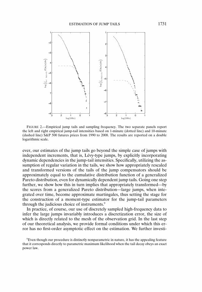
The importance of using high-frequency data to effectively estimate the largejumps and the power-law decay for the intensities is clearly illustrated by Fig-ure 2, which compares the empirical jump tails for the S&P 500 market portfo-lio estimated with 1- and 10-minute returns, respectively. While the estimatescoincide for the larger jump sizes, as they should, our ability to meaningfullyextract the more moderate-sized jumps obviously becomes more limited at the10-minute frequency. Intuitively, the coarser is the sampling frequency, themore the continuous variation will obscure the jumps and the greater cutoffvalues will need to be used in the jump-tail inference, in turn resulting in a lossof jump observations and efficiency of the estimation.8
Figures 1 and 2 both corroborate the empirical validity of the assumedpower-law decay underlying our asymptotic approximations. Importantly, how-
5Another advantage of working directly with the jumps is that our estimator does not dependon the form of the stochastic volatility and, in particular, is robust to the presence of jumps inthe volatility, as explored parametrically by Barndorff-Nielsen and Shephard (2001) and morerecently using nonparametric procedures by, for example, Jacod and Todorov (2010) and Todorovand Tauchen (2011).
6Shimizu (2006) and Shimizu and Yoshida (2006) also previously relied on similar methods inthe parametric estimation of jump-diffusion models.
7They imply, among other things, that the jump-tail intensities should obey a power law forsufficiently large jump sizes. Formally, this result builds on the so-called peaks-over-thresholdmethod together with the assumption of regular variation in the tails, as originally developed bySmith (1987) in the context of independent and identically distributed (i.i.d.) random variables.
8Of course, the use of coarser daily frequency returns, as commonly done in the estimation ofparametric jump-diffusion models, would even further exaggerate these same effects and handi-cap the detection of jumps.
ESTIMATION OF JUMP TAILS 1731
FIGURE 2.—Empirical jump tails and sampling frequency. The two separate panels reportthe left and right empirical jump-tail intensities based on 1-minute (dotted line) and 10-minute(dashed line) S&P 500 futures prices from 1990 to 2008. The results are reported on a doublelogarithmic scale.
ever, our estimates of the jump tails go beyond the simple case of jumps withindependent increments, that is, Lévy-type jumps, by explicitly incorporatingdynamic dependencies in the jump-tail intensities. Specifically, utilizing the as-sumption of regular variation in the tails, we show how appropriately rescaledand transformed versions of the tails of the jump compensators should beapproximately equal to the cumulative distribution function of a generalizedPareto distribution, even for dynamically dependent jump tails. Going one stepfurther, we show how this in turn implies that appropriately transformed—bythe scores from a generalized Pareto distribution—large jumps, when inte-grated over time, become approximate martingales, thus setting the stage forthe construction of a moment-type estimator for the jump-tail parametersthrough the judicious choice of instruments.9
In practice, of course, our use of discretely sampled high-frequency data toinfer the large jumps invariably introduces a discretization error, the size ofwhich is directly related to the mesh of the observation grid. In the last stepof our theoretical analysis, we provide formal conditions under which this er-ror has no first-order asymptotic effect on the estimation. We further investi-
9Even though our procedure is distinctly nonparametric in nature, it has the appealing featurethat it corresponds directly to parametric maximum likelihood when the tail decay obeys an exactpower law.

1732 T. BOLLERSLEV AND V. TODOROV
gate the accuracy of these asymptotic-based approximations through a seriesof Monte Carlo simulations, confirming the applicability of the feasible versionof the new jump-tail estimation procedure.
On actually implementing the estimators with the same high-frequency S&P500 data that underlies the average jump-tail intensities depicted in the figuresdiscussed above, we find strong evidence for temporal variation in the jumpintensities, and much richer and more complex dynamic dependencies in theresulting jump tails than hitherto entertained in the literature. As such, the neweconometric modeling framework developed in this paper has the potential toallow for jump-tail forecasting and, in turn, can be used to provide a deepereconomic understanding of the tail events of the types observed during therecent financial crisis.
The rest of the paper is organized as follows. Section 2 introduces the basicnotation and key assumptions. Section 3 describes the main idea behind thenew estimation method and the relevant asymptotic results when continuousprice records are available. Section 4 extends the analysis to the practically rel-evant situation of discretely sampled prices. The practical applicability of thenew estimator is confirmed through a series of Monte Carlo simulations pre-sented in Section 5. Section 6 discusses the empirical estimation results for theS&P 500 market index and our findings related to the rich dynamic dependen-cies inherent in the jump tails of that portfolio. Section 7 concludes. All proofsare deferred to Section 8. Computer codes for performing the estimation inthe paper can be found in the supplementary material (Bollerslev and Todorov(2011b)).
2. SETUP AND ASSUMPTIONS
To set up the notation, let pt := ln(Pt) denote the logarithmic price of afinancial asset. We assume that the log price follows an Itô semimartingaledefined on some filtered probability space, that is,
dpt = αt dt + σt dWt +∫
R
κ(x)μ(dt�dx)+∫
R
κ′(x)μ(dt�dx)�(2.1)
where αt and σt are both locally bounded processes; Wt denotes a Brownianmotion; μ is a one-dimensional measure on [0�∞)×R that counts the numberof jumps of given size x over a given time interval; the compensator of the jumpmeasure is denoted by νt(x)dxdt, where μ(dt�dx) := μ(dt�dx)− νt(x)dxdtrefers to the corresponding compensated measure; and κ(x) is a continuousfunction with bounded support equal to x around the origin, with κ′(x)= x−κ(x).10 We also assume throughout that νt(dx) is absolutely continuous withrespect to Lebesgue measure, that is, νt(dx)= νt(x)dx. The main contributionof this paper is to provide a new, essentially model-free, robust framework
10The two separate integrals on the right-hand side of equation (2.1) reflect the different sta-tistical properties of small and large jumps. In general, small jumps may be of infinite variation

ESTIMATION OF JUMP TAILS 1733
for the estimation of the tail behavior of νt(x), leaving other aspects of thedata generating process in equation (2.1), including the drift term αt and thestochastic volatility σt , as well as the activity level of the jumps, unspecifiedand free to instantly vary. We do assume, however, that conditional on pastinformation, the large-sized jumps are identically distributed.
Finance theory, under mild regularity conditions, implies that all asset pricesshould be semimartingales. Formally, the only additional assumption imposedby the representation in equation (2.1) is that the characteristics of the semi-martingale, that is, the drift term, the quadratic variation of the diffusion, andthe compensator for the jump measure, are all absolutely continuous in timeprocesses. This assumption is satisfied by virtually all of the processes hith-erto used in the asset pricing literature. It does, however, rule out certainprocesses where the Brownian motion is time-changed by a separate discon-tinuous process.11
As noted in the Introduction, the existing evidence concerning the empiri-cal features of νt(x) for large values of the jump sizes x come almost exclu-sively from tightly parameterized jump-diffusion models. In particular, follow-ing Merton (1976), most empirical studies to date have relied on relativelysimple and tractable compound Poisson jump processes with normally distrib-uted jump sizes. Under this specification, the Lévy measure in equation (2.1)can be expressed as νt(x) = λte−(x−μ)2/(2σ2)(2πσ2)−1/2, where λt denotes somepredictable stochastic process intended to capture the time-varying probabilityof jump arrivals, typically postulated to be a linear function of the stochasticvolatility σ2
t−. While such a formulation is very convenient from an analyticalperspective, Figure 1 above clearly shows that such a specification does notnecessarily fit the tails very well.
As also noted in the Introduction, another problem with fully parametricapproaches to estimating the jump tails is that they generally link the behaviorof the small and the large jumps in a highly model-specific fashion. Statistically,however, the small and the large jumps are very different. The behavior ofthe Lévy measure around 0 and the corresponding first integral on the right-hand side of equation (2.1) capture mainly the pathwise properties of the jumpprocess; for example, finite or infinite activity and finite or infinite variation. Bycontrast, the last term in equation (2.1) and the jump tails only depend on thelarge jumps. Indeed, our basic minimal assumptions related to νt(x), as stated
and the corresponding integration is defined in a stochastic sense with respect to the martingalemeasure μ. This directly mirrors the integral that naturally arises for the diffusive increments withrespect to the Brownian motion, which is similarly an infinite variation process. By contrast, thereis only a finite number of large jumps over a given finite time interval, and the second integrationis consequently defined in the usual Riemann–Stieltjes sense.
11In practice, a host of market microstructure frictions also prevent us from directly observingthe efficient price. As discussed in more detail below, our empirical strategy for dealing with thisis to rely on appropriately chosen discrete sampling frequency, so that the effect of the measure-ment error in the actually observed price process vis-à-vis the one defined by equation (2.1) isnegligible.

1734 T. BOLLERSLEV AND V. TODOROV
in A1 and A2 immediately below, only concern the behavior of the large jumpsand put no restrictions on the jump activity per se.
ASSUMPTION A1: The jump compensator νt(x) satisfies
νt(x)= (ϕ+t 1{x>0} +ϕ−
t 1{x<0})ν(x)�(2.2)
where ϕ±t are nonnegative-valued stochastic processes with cadlag paths and ν(x)
is a positive measure on R with∫
R(|x|2 ∧ 1)ν(x)dx <∞.
Assumption A1 factors the dependence in the jump compensator on time (t)and jump size (x) into two separate functions. This implies that differentlysized jumps will have the same dynamic properties. Intuitively, in the case offinite activity jumps, the assumption implies that we allow for a different timechange for the positive and negative jumps, but otherwise leave the distributionthe same. Most parametric jump specifications used to date, for example, time-changed Lévy processes, trivially satisfy this assumption. Still, the assumptionis slightly stronger than what we actually need, and it would be possible torelax A1 to hold only for sufficiently large values of |x|. However, to avoid theunnecessary additional complications that arise in this situation, we maintainA1 in its current form.
Our interest centers on the tail behavior of the Lévy density ν(x), whichin turn determines the tail behavior of the jumps in the price process. Ournext assumption concerns the variation in the tails of ν(x) and is directly mo-tivated by the apparent power tail decay seen in Figure 1 and discussed in theIntroduction. To facilitate our analysis and the notation, define the functionsψ(x) := e|x| − 1, and
ψ+(x) :={ψ(x)� x > 0,0� x≤ 0, ψ−(x) :=
{0� x > 0,ψ(x)� x≤ 0.
These functions allow us to switch from jumps in the log price to jumps in lev-els. Also, denote ν+
ψ(y) = ν(ln(y+1))y+1 and ν−
ψ(y) = ν(− ln(y+1))y+1 for y ∈ (0�∞). Then
for every measurable set A in (0�∞), ∫(0�∞) 1{x∈A}ν+
ψ(x)dx= ∫R+ 1{ex−1∈A}ν(x)dx
and∫(0�∞) 1{x∈A}ν−
ψ(x)dx = ∫R− 1{e−x−1∈A}ν(x)dx. Moreover, denote the tails of
the measures by ν±ψ(x) := ∫ ∞
xν±ψ(u)du for some x > 0. The functionψ(x)maps
the positive and negative jumps to (0�∞), with the Lévy densities for the trans-formed jumps given by the ν±
ψ measures. Assumption A2 imposes regular vari-ation for the tails of the latter.
ASSUMPTION A2:(a) Functions ν±
ψ(x) are regularly varying at infinity, that is, ν±ψ(x) =
x−α±L±(x), where α± > 0 and L±(x) are slowly varying at infinity.12
12A function L(x) is said to be slowly varying at infinity if limx→∞ L(tx)L(x)
= 1 for every t > 0.

ESTIMATION OF JUMP TAILS 1735
(b) Functions L±(x) satisfy the condition L±(tx)/L±(x)= 1 +O(τ±(x)) asx ↑ ∞ for t > 0, where τ±(x) > 0, τ±(x)→ 0 as x ↑ ∞, and τ±(x) are nonin-creasing.
Assumption A2 is key to our analysis and several comments are in order.First, the close to linear behavior of the empirical jump-tail estimates forthe large jumps depicted in Figure 1 is directly in line with A2(a). Second,A2(a) rules out Lévy measures with light tails, that is, Merton-type jumps,whose tails belong in the maximum domain of attraction of the Gumbel dis-tribution; see, for example, Embrechts, Kluppelberg, and Mikosch (2001).13
Third, the decay of the tail measures ν±ψ(x) is directly linked to the fat-
tailedness of the transformed jumps ψ(�pt). In particular, the integrabilityof
∫ t+at
∫R|ψ(x)|pμ(ds�dx) depends on whether p ≷ α±. Assumption A2(a)
therefore implies that all powers of the jumps in the logarithmic price exist.Alternatively, one could assume that A2(a) holds for ν±(x) instead of ν±
ψ(x),where ν+(x)= ∫ ∞
xν(u)du and ν−(x)= ∫ −x
−∞ ν(u)du for x > 0, or equivalently,that the continuously compounded returns ln( pt
pt− ), instead of the “discrete” re-turns Pt−Pt−
Pt− , should be modeled with Lévy densities with power decay in theirtails. We think the former is less appealing from an economic perspective.14
Assumption A2(b) is taken directly from Smith (1987); see also Goldie andSmith (1987). It essentially limits the deviation of the tail measures ν±
ψ(x) fromthe power law. We use this assumption in determining the rate of convergenceand establishing asymptotic normality of the estimates for the jump-tail prob-abilities.
Our next assumption imposes minimal stationarity and integrability condi-tions on ϕ±
t . This assumption is needed to ensure that the standard long-spanasymptotics works in conjunction with the other assumptions to consistentlyinfer the jump tails.
ASSUMPTION A3: Processes ϕ±t are stationary and satisfy 0 < E|ϕ±
t |1+ε < Kfor some K > 0 and ε > 0.
Our final assumption restricts ϕ±t to be an Itô semimartingale. It also im-
poses some weak additional integrability conditions on the stochastic processes
13Although the new estimation method could be adopted to cover this case as well, parts ofthe proof would require slightly different techniques. Since this case arguably is not empiricallyrelevant, we do not consider it here.
14Assuming a heavy-tailed distribution for the continuously compounded returns would implyan infinite conditional variance for the price level, which in turn can result in infinite option pricesand, as conjectured by Merton (1976), might also result in infinite equilibrium interest rates. Inpractice, of course, it is impossible to differentiate whether Assumption A2(a) holds for ν±
ψ(x) orν±(x), as the difference between ln( pt
pt− ) and Pt−Pt−Pt− is numerically very small for the jump sizes
that we actually observe.
1736 T. BOLLERSLEV AND V. TODOROV
that appear in the definition of the price process in equation (2.1). We need thisassumption in the empirically realistic situation when the price is only observedat discrete points in time.
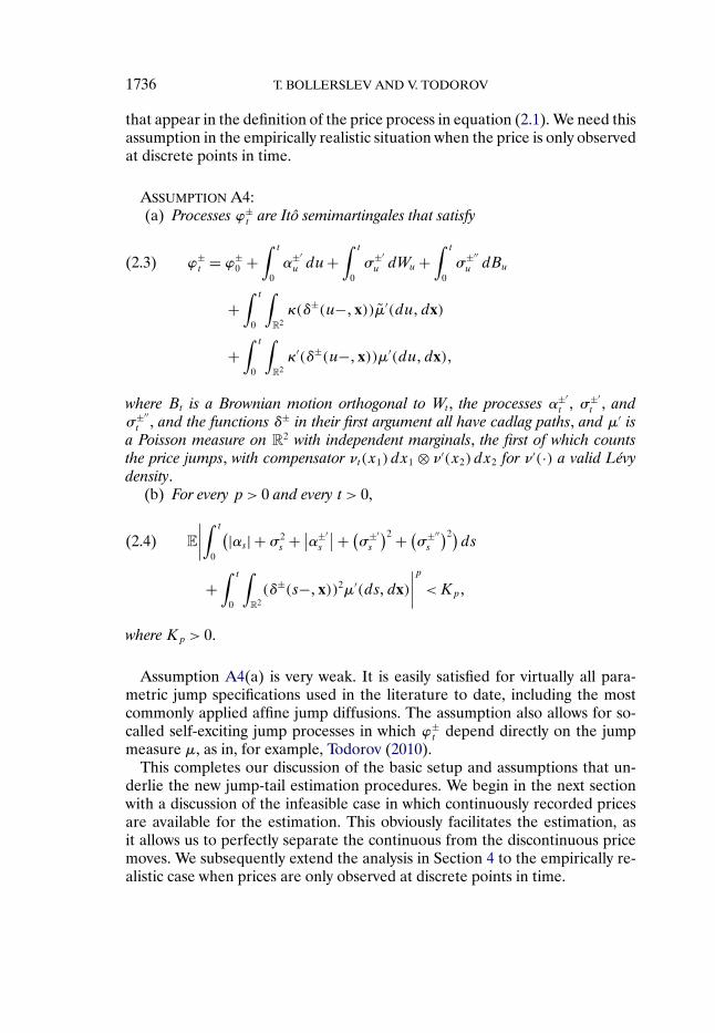
ASSUMPTION A4:(a) Processes ϕ±
t are Itô semimartingales that satisfy
ϕ±t = ϕ±
0 +∫ t
0α±′u du+
∫ t
0σ±′u dWu +
∫ t
0σ±′′u dBu(2.3)
+∫ t
0
∫R2κ(δ±(u−�x))μ′(du�dx)
+∫ t
0
∫R2κ′(δ±(u−�x))μ′(du�dx)�
where Bt is a Brownian motion orthogonal to Wt , the processes α±′t , σ±′
t , andσ±′′t , and the functions δ± in their first argument all have cadlag paths, and μ′ is
a Poisson measure on R2 with independent marginals, the first of which countsthe price jumps, with compensator νt(x1)dx1 ⊗ ν′(x2)dx2 for ν′(·) a valid Lévydensity.
(b) For every p> 0 and every t > 0,
E
∣∣∣∣∫ t
0
(|αs| + σ2s + ∣∣α±′
s
∣∣+ (σ±′s
)2 + (σ±′′s
)2)ds(2.4)
+∫ t
0
∫R2(δ±(s−�x))2μ′(ds�dx)
∣∣∣∣p <Kp�
where Kp > 0.
Assumption A4(a) is very weak. It is easily satisfied for virtually all para-metric jump specifications used in the literature to date, including the mostcommonly applied affine jump diffusions. The assumption also allows for so-called self-exciting jump processes in which ϕ±
t depend directly on the jumpmeasure μ, as in, for example, Todorov (2010).
This completes our discussion of the basic setup and assumptions that un-derlie the new jump-tail estimation procedures. We begin in the next sectionwith a discussion of the infeasible case in which continuously recorded pricesare available for the estimation. This obviously facilitates the estimation, asit allows us to perfectly separate the continuous from the discontinuous pricemoves. We subsequently extend the analysis in Section 4 to the empirically re-alistic case when prices are only observed at discrete points in time.

ESTIMATION OF JUMP TAILS 1737
3. ESTIMATION OF JUMP TAILS: CONTINUOUS PRICE RECORDS
The basic idea behind our estimation scheme builds on the three assump-tions in A1–A3 and the relevant extreme value theory-type approximations forappropriately transformed versions of the jump tails. The common approachfor assessing tail behavior in extreme value theory relies on discretely sampledprices, or returns, and a corresponding estimate of the tail index; see, for exam-ple, Embrechts, Kluppelberg, and Mikosch (2001) and the references therein.Importantly, however, we are after the tail behavior of the jump measure μitself, as opposed to that of the discrete returns.15
In general, there is no direct link between the tails of the discrete returns andthe Lévy measure of the price process. For one, time-varying volatility in thecontinuous part of the price process, as determined by σt , invariably impactsthe tails of the discrete returns.16 Second, temporal dependencies in the jumpintensity itself, that is, the dependence of νt(x) on t, also affect the tails. Whileit would be possible to circumvent the first problem in the continuous-recordcase by looking only at the jump increments, any time variation in the jumpintensity would still blur the link between the tails of the latter and the tails ofν(x) in the decomposition in A1.
Instead, we base our inference directly on the jumps or, in the case of dis-cretely observed prices, estimates thereof, and a set of moment conditions forthe jump intensity νt(x) derived from Assumptions A1 and A2. Using the factthat the random jump measure μ differs from its compensator by a martingale,we translate the moment conditions for νt(x) to a set of moment conditions forμ that involve the estimated in-sample jumps. To conserve space, we focus ourdiscussion on the estimation of the right tail only; the estimation of the left tailproceeds completely analogously.
We begin by approximating the distribution of 1 − ν+ψ(y)ν+ψ(x)
for y ≥ x > 0 using
A1 and A2. We then rely on the scores from this approximating distribution todefine a set of feasible estimating equations based on the observed large jumps.This idea originates in the so-called peaks-over-thresholds method for estimat-ing the tails and the tail decay of i.i.d. random variables originally developedby Smith (1987). Specifically, it follows from Assumption A2 that
ν+ψ(u+ x)ν+ψ(x)
=(
1 + u
x
)−α+
+(
1 + u
x
)−α+(L+(x+ u)L+(x)
− 1)�(3.1)
15Under fairly general conditions, the tail of discrete increments from a Lévy process is pro-portional to the tail of its Lévy measure; see, for example, Rosinski and Samorodnitsky (1993,Theorem 2.1). Intuitively, since the continuous part of any Lévy increment is normal, its contri-bution becomes negligible “deep” in the tail.
16As shown by Leadbetter and Rootzen (1988), the extremes of two sequences of discretereturns with the same marginal law, one with and the other without any temporal dependencies,is generally different.

1738 T. BOLLERSLEV AND V. TODOROV
where u > 0 and x > 0. Since L+(·) is a slowly varying at infinity function, thesecond term becomes negligible for large x. Thus,
1 − ν+ψ(u+ x)ν+ψ(x)
∼G(u;σ+� ξ+)(3.2)
= 1 − (1 + ξ+u/σ+)−1/ξ+� ξ+ �= 0�σ+ > 0�
where G(u;σ+� ξ+) denotes the cumulative distribution function (c.d.f.) of ageneralized Pareto distribution with parameters σ+ = x
α+ and ξ+ = 1α+ , and the
tail decay parameter α+ is determined by A2(a). Let the scores associated withthe log-likelihood function of the generalized Pareto distribution be denotedby
φ+1 (u�σ
+� ξ+)= 1ξ+ −
(1 + 1
ξ+
)(1 + ξ+u
σ+
)−1
�(3.3)
φ+2 (u�σ
+� ξ+)= 1(ξ+)2
log(
1 + ξ+uσ+
)− 1ξ+
(1 + 1
ξ+
)
+ 1ξ+
(1 + 1
ξ+
)(1 + ξ+u
σ+
)−1
�
where i= 1�2 refers to the derivatives with respect to σ+ and ξ+, respectively.The idea is then to pick a large threshold �T and to fit the scores to the
jumps above this threshold. Doing so results in the set of moment conditionsinvolving the realized large jumps,
gT (�T )(3.4)
= 1M+T
×T−1∑t=1
⎛⎜⎜⎝∫ t+1
t
∫R
φ+1
(ψ(x)−�T�θ(1)� θ(2)
)1{ψ+(x)>�T }μ(ds�dx)∫ t+1
t
∫R
φ+2
(ψ(x)−�T�θ(1)� θ(2)
)1{ψ+(x)>�T }μ(ds�dx)
⎞⎟⎟⎠ �where θ denotes the 2 × 1 vector of unknown parameters and M+
T equals thenumber of positive in-sample jumps which, upon transformation by ψ(·), ex-ceed the threshold �T , that is,17
M+T =
T−1∑t=1
∫ t+1
t
∫R
1{ψ+(x)>�T }μ(ds�dx)�(3.5)
17M+T provides an estimate for Tν+
ψ(�T )E(ϕ+t ).

ESTIMATION OF JUMP TAILS 1739
In theory, of course, �T will have to grow to infinity with the sample size T .Denote the true parameter values implicitly defined by the moment conditionsθ0T = (σ+
T � ξ+)′, where σ+
T = �Tα+ increases with the sample size T . We then have
the following theorem.18
THEOREM 1: For the process pt defined in (2.1), assume that A1–A3 hold. Letthe sequence of truncation levels satisfy
�T → ∞� Tν+ψ(�T)→ ∞� and(3.6) √
Tν+ψ(�T )τ
+(�T )→ 0 as T → ∞�
where τ+(·) is defined in A2(b). Then, for T → ∞, with probability approaching 1,gT (θ��T )= 0 has a solution θT := (σ+
T � ξ+)′, which satisfies√
M+T
(σ+T /σ
+T − 1
ξ+ − ξ+
)L→ Σ−1/2Z�(3.7)
Σ= 1(α+ + 1)(α+ + 2)
(α+(α+ + 1) (α+)2
(α+)2 2(α+)2
)where Z denotes a standard bivariate normal distribution.
The scaling factor for the difference between the estimated and the trueparameters that control the tails is given by the random numberM+
T . Of course,M+T /(Tν
+ψ(�T ))
P→ E(ϕ+t ) and Tν+
ψ(�T ) is nonrandom. However, since ν+ψ(�T )
converges to 0, the rate of convergence is, in general, slower than the standard√T rate. In particular, it follows from the conditions for the truncation level
in (3.6) that the larger are the deviations of the tail from the power-law decay,that is, the slower is the rate at which τ+(x) goes to zero as x ↑ ∞, the sloweris the rate of convergence of the estimator. Intuitively, the farther are the tailsfrom the eventual power-law decay, the larger is the required truncation level,which in turn slows down the rate of convergence as fewer observations areemployed in the estimation.
To further appreciate this result, suppose that τ+(x) = |x|−k for somek > 0. In this situation, the required rate condition in (3.6) stipulates that�T =O(T 1/(α++2k)), so that for k→ ∞, that is, L+(x) in A2 converging to unityand diminishing deviations from the power law, it is possible to get arbitrarily
18Alternatively, we could have used the score based on the approximationν+ψ(u+x)ν+ψ(x)
appr∼ (1 +ux)−1/ξ+
� ξ+ �= 0� obtained by substituting the true value of σ+ = xα+ in equation (3.2). This would
involve only a single parameter and it could be seen as an analogue of Hill’s (1975) estimatorin the jump-tail setting. However, such an estimator would not be scale-free and the analysis inSmith (1987) also suggests that it would be less robust than the estimator advocated in Theorem 1.

1740 T. BOLLERSLEV AND V. TODOROV
close to the standard parametric√T rate of convergence for optimally chosen
�T .In practice, of course, we do not know a priori the form of the slowly varying
function L+(x) that dictates the optimal choice of the truncation level, andwe are faced with a trade-off in terms of robustness versus efficiency in theestimation. A low value of �T would entail the use of more observations, thatis, more jumps, and hence a more efficient estimator. On the other hand, bychoosing �T too small, we run the risk of larger deviations from the eventualpower-law tail decay and nonrobustness of the estimation. We explore thesetrade-offs more fully in the Monte Carlo simulations reported in Section 5below.
Importantly, the estimating equations in (3.4) correctly identify the tail be-havior of ν(x), even in the presence of time-varying jump intensities. Intu-itively, temporal dependence in the jump intensity does not affect the distri-bution of the large jumps, and as such the presence of more jumps in certainperiods does not systematically bias the estimator. By contrast, any estimatorbased on the jump increments over fixed intervals of time, for example, days,would invariably be affected by jump clustering and a failure to properly ac-count for that effect would result in biased tail index estimates.
Even though Theorem 1 allows for jump clustering, it does not fully exploitthe dynamic structure of the jump tails implied by Assumptions A1 and A2.Going one step further, it follows from the proofs in the Section 8 that fort� s ≥ 0,19
Et
(∫ t+s
t
∫R
φ+i
(ψ(x)−�T�θ(1)� θ(2)
)μ(du�dx)
)= Et
(∫ t+s
t
∫R
φ+i
(ψ(x)−�T�θ(1)� θ(2)
)μ(du�dx)
)+
∫R
φ+i
(ψ(x)−�T�θ(1)� θ(2)
)ν(x)dxEt
(∫ t+1
t
ϕ+u du
)=
∫R
φ+i
(ψ(x)−�T�θ(1)� θ(2)
)ν(x)dxEt
(∫ t+s
t
ϕ+u du
)≈ 0�
where we have used the shorthand notation Et(·)= E(·|Ft). In particular, forany instrument xt adapted to Ft ,
E
(xt
∫ t+1
t
∫R
φ+i
(ψ(x)−�T�θ(1)� θ(2)
)μ(ds�dx)
)≈ 0�
This in turn suggests the following extension of Theorem 1.
19Recall that the counting jump measure μ is not a martingale, but that its compensation ver-sion, μ(ds�dx)= μ(ds�dx)− νt(x)dxdt, is.

ESTIMATION OF JUMP TAILS 1741
THEOREM 2: For the process pt defined in (2.1), assume that A1–A3 hold. Letthe sequence of truncation levels satisfy the growth condition (3.6) of Theorem 1.Define the vector of moment conditions
gT (�T )(3.8)
= 1M+T
T−1∑t=1
xt
⊗
⎛⎜⎜⎝∫ t+1
t
∫R
φ+1
(ψ(x)−�T�θ(1)� θ(2)
)1{ψ+(x)>�T }μ(ds�dx)∫ t+1
t
∫R
φ+2
(ψ(x)−�T�θ(1)� θ(2)
)1{ψ+(x)>�T }μ(ds�dx)
⎞⎟⎟⎠ �where xt is a q×1 Ft-adapted stationary vector process that satisfies E‖xt‖2+ε <∞for some ε > 0 such that a law of large numbers holds for 1
T
∑T−1t=1 xt
∫ t+1tϕ+s ds
and 1T
∑T−1t=1 xtx′
t
∫ t+1tϕ+s ds with E(xt
∫ t+1tϕ+s ds) �= 0 as T → ∞. Further, let WT
denote a sequence of symmetric positive semi-definite 2q × 2q matrices suchthat WT
P→ W , where W is a 2q × 2q positive definite matrix. Denote θT =arg minθ∈ΘlT gT (θ��T)
′WTgT (θ��T), where ΘlT = {θ :αlθ
0(i)T ≤ θ(i) ≤ αhθ0(i)
T � i =1�2} for some constants 0< αl < 1< αh. Then, for T → ∞, θT exists with prob-ability approaching 1 and√
M+T
(σ+T /σ
+T − 1
ξ+ − ξ+
)L→
√E(ϕ±
t )Ξ1/2Z�(3.9)
Ξ = (Π′WΠ)−1(Π′W V WΠ)(Π′WΠ)−1�
where Z is a standard bivariate normal distribution,
Π = E
(xt
∫ t+1
t
ϕ+s ds
)⊗Σ� V = E
(xtx′
t
∫ t+1
t
ϕ+s ds
)⊗Σ�(3.10)
and Σ is defined in (3.7).
The use of additional instruments in the estimation of the tail parameters af-forded by Theorem 2 provides a general and convenient framework for testingthe dynamic structure of the jumps. In the semiparametric example discussedin the next subsection, we provide a practically attractive choice for the in-strument vector process xt . A consistent estimate of the variance–covariancematrix for the resulting parameter estimates is readily obtained by replacingeach of the relevant matrices in the expression for Ξ in equation (3.9) with
ΠT =T−1∑t=1
xt
∫ t+1
t
∫ψ+(x)>�T
μ(ds�dx)⊗ ΣT �

1742 T. BOLLERSLEV AND V. TODOROV
VT =T−1∑t=1
xtx′t
∫ t+1
t
∫ψ+(x)>�T
μ(ds�dx)⊗ ΣT �
and replacing ΣT defined from Σ in equation (3.7) with α+ estimated by 1/ξ+.Thus far our focus has centered on recovering the tail properties of ν(x).
In most practical applications, however, one would be interested in the tailsof νt(x). Building on the decomposition for νt(x) in Assumption A1 into itstime-varying components ϕ±
t , it follows that for the large jumps, the difference∫ t
0
∫R
φ(s−�x)μ(ds�dx)−∫ t
0
∫R
φ(s−�x)ϕ+s dsν(x)dx
must be a martingale for any function φ(s�x) with cadlag paths, and φ(s�x)=0 for x < K, where K > 0 denotes some constant. In parallel to the discus-sion above, this therefore allows for the construction of a set of unconditionalestimating equations through the appropriate choice of instrument(s) xt . Ingeneral, of course, the resulting moments depend on the exact specification ofthe ϕ±
t processes. To illustrate, we next consider the special case in which thetime-varying part of the right jump intensity is assumed to be an affine functionof the spot variance, that is, ϕ+
t = k+0 + k+
1 σ2t . This same basic assumption also
underlies our empirical illustration in Section 6 below.
3.1. Affine Jump Intensities
The assumption that the temporal dependencies in the jump intensities areaffine in the spot volatility nests virtually all parametric jump-diffusion modelshitherto considered in the literature, including the affine jump-diffusion classof models popularized by Duffie, Pan, and Singleton (2000). Importantly, how-ever, by making no parametric assumptions about the volatility process itself,the semiparametric setup adopted here is much more flexible, allowing for thepossibility of so-called self-exciting jumps and models in which σt depends onthe jump measure μ.
The maintained assumption of continuous price records underlying all of theresults in this section and our ability to perfectly identify the large jumps simi-larly allows us to perfectly infer the integrated variation
∫ tt−1σ
2s ds. In practice,
as discussed further below, with discretely observed prices, estimates of the in-tegrated variation invariably involve some estimation error. Nonetheless, thisnaturally suggests using that measure to help identify the dependence of ϕ+
t onσ2t . The following corollary extends the results above to cover this situation.
COROLLARY 1: For the process pt defined in (2.1), assume that A1–A3 holdand thatϕ+
t = k+0 +k+
1 σ2t . Denote θ= (σ+� ξ+�k+
0 ν+ψ(�T )�k
+1 ν
+ψ(�T )) and define

ESTIMATION OF JUMP TAILS 1743
the vector of moment conditions
gT (�T )(3.11)
= 1M+T
T−1∑t=1
xt
⊗
⎛⎜⎜⎜⎜⎜⎜⎜⎝
∫ t+1
t
∫R
φ+1
(ψ(x)−�T�θ(1)� θ(2)
)1{ψ+(x)>�T }μ(ds�dx)∫ t+1
t
∫R
φ+2
(ψ(x)−�T�θ(1)� θ(2)
)1{ψ+(x)>�T }μ(ds�dx)∫ t+1
t
∫ψ+(x)>�T
μ(ds�dx)− θ(3) − θ(4)∫ t+1
t
σ2s ds
⎞⎟⎟⎟⎟⎟⎟⎟⎠with xt = (1
∫ tt−1σ
2s ds )
′. Assume that the growth condition for �T in (3.6) issatisfied and that a law of large numbers holds for 1
T
∑T−1t=1
∫ tt−1σ
2s ds
∫ t+1tσ2s ds
and 1T
∑T−1t=1 (
∫ tt−1σ
2s ds)
2∫ t+1tσ2s ds as T → ∞, with E|σt |6+ε <∞ for some ε > 0.
Finally, let WT denote a sequence of symmetric positive semidefinite 6×6 matricessuch that WT
P→W , where W is a 6 × 6 positive definite matrix, and denote θT =arg minθ∈ΘlT gT (θ��T)
′WTgT (θ��T).(a) Then for T → ∞, the estimator θT exists with probability approaching 1
and
√M+T
⎛⎜⎜⎜⎜⎝σ+T /σ
+T − 1
ξ+ − ξ+
k+0 ν
+ψ(�T)/ν
+ψ(�T)− k+
0
k+1 ν
+ψ(�T)/ν
+ψ(�T)− k+
1
⎞⎟⎟⎟⎟⎠ L→√
E(ϕ±t )Ξ
1/2Z�
where Z is a standard multivariate normal, Ξ = (Π′W Π)−1(Π′W V W Π) ×(Π′W Π)−1 with
Π =
⎛⎜⎜⎝Π 04×2
02×2
⎛⎝ 1 Eσ2t
Eσ2t E
(∫ t
t−1σ2s ds
∫ t+1
t
σ2s ds
)⎞⎠⎞⎟⎟⎠ �
V =⎛⎝ V 02×2
02×2 E
(xtx′
t
∫ t+1
t
(k+0 + k+
1 σ2s ) ds
)⎞⎠ �and Π and V defined in (3.10).

1744 T. BOLLERSLEV AND V. TODOROV
(b) Further, let zT = η�T for some constant η≥ 1 and denote
k+i ν
+ψ(zT )= k+
i ν+ψ(�T)
(1 + ξ+
σ+T
(zT −�T))−1/ξ+
� i= 0�1�(3.12)
Then, for T → ∞,√M+T
(k+
0 ν+ψ(zT )/ν
+ψ(zT )− k+
0
k+1 ν
+ψ(zT )/ν
+ψ(zT )− k+
1
)L→ (ΦΞΦ′)1/2Z�(3.13)
where
Φ=(k+
0 α+η−α+−1(η− 1) k+
0 (α+)2η−α+
(log(η)− 1 + 1/η) η−α+0
k+1 α
+η−α+−1(η− 1) k+1 (α
+)2η−α+(log(η)− 1 + 1/η) 0 η−α+
)(3.14)
and Z refers to the standard normal vector from part (a).
The last two moment conditions effectively serve to disentangle the constantand time-varying parts, that is, k+
0 ν+ψ(�T ) and k+
1 ν+ψ(�T ), respectively. They
may be interpreted as linear projections of the counts of large jumps on a con-stant and the integrated variation over the previous period. As such, these twomoment conditions only require that the affine structure holds for the largejumps. Part (b) of the corollary shows how the estimation framework can beextended to meaningfully characterize the behavior of the jump tails at levelsfor which we (invariably) have few in-sample observations. These, of course,are also the levels of interest in many risk management situations involvingextreme value-at-risk–type quantities. We further illustrate this important newdimension of our result in the empirical application discussion in Section 6below.
Our formal analysis up until now has been based on the assumption of con-tinuously recorded prices. We next discuss how this empirically unrealistic as-sumption can be relaxed and the results extended to the case when prices areonly observed at discrete points in time.
4. ESTIMATION OF JUMP TAILS: DISCRETELY SAMPLED PRICES
The results in the previous section relied on our ability to directly identifythe jumps in a continuously observed realization of the underlying process.The theoretical notion of continuous price records is, of course, practicallyinfeasible. Instead, we now assume that over each unit time interval [t� t + 1],the price process pt is “only” observed at the discrete points in time t� t +Δn� � � � � t+nΔn for some Δn > 0. We refer to n= [1/Δn] as the number of high-frequency price observation over the “day.” To facilitate the exposition, we usethe shorthand notation Δn�ti p := pt+iΔn −pt+(i−1)Δn to refer to the correspondingprice increments.

ESTIMATION OF JUMP TAILS 1745
To adapt the same basic estimation strategies to the case of high-frequencydata, we assume that the length of the sampling interval goes to zero, that is,Δn → 0.20 This allows us, at least in some limiting sense, to estimate the largejumps and, in turn, to construct feasible estimates of the same integrals withrespect to the jump measures and corresponding moment conditions analyzedabove, say gT (θ��T ). These high-frequency based estimates, of course, containdiscretization errors, but we show that under appropriate conditions, the errorsshrink to zero and do not affect the estimates.
In particular, our estimates for the integrals∫ t+1t
∫ψ+(x)>�T φ
+i (ψ(x)−�T �θ(1)�
θ(2))μ(ds�dx), i= 1�2, can simply be expressed as21
n∑j=1
φ+i
(ψ(Δn�tj p)−�T�θ(1)� θ(2)
)1(ψ+(Δn�tj p) > �T)� i= 1�2�
These expressions rely on the fact that for the estimation of the tails, we onlyneed to evaluate the score functions φ+
i for values of |x| outside a neighbor-hood of zero. More formally, using the modulus of continuity of cadlag func-tions, all but the high-frequency intervals containing the large jumps can bemade arbitrarily small uniformly over a given fixed time interval, and thoseincrements, therefore, do not matter in the estimation of the integrals with re-spect to the jump measure. This argument, of course, is only pathwise, and inour analysis, the time span T also increases as Δn goes to zero. This requiressomewhat different arguments in the formal proof, but the intuition remainsthe same.22
Altogether this implies that the feasible estimation with discretely sampledhigh-frequency prices will be subject to three distinct types of errors, namely(i) the sampling error associated with the empirical processes employed in themoment vector, controlled by the span of the data T , (ii) approximation er-ror for the jump tail, controlled by the truncation size �T , and (iii) discretiza-tion error from “filtering” the jumps from the high-frequency data, controlledby the length of the high-frequency interval Δn or, equivalently, the numberof high-frequency observations per unit time interval n. The following theo-rem provides rate conditions for the relative speeds with which T , �T , and nincrease that are sufficient to ensure that the feasible estimation remains as-ymptotically equivalent to the infeasible procedures discussed in the previoussection.
20The assumption of equally spaced observations is not critical, but the assumption that thelargest mesh size goes to zero, or Δn → 0 in the case of equidistant observations, is.
21In actually implementing the estimating equations below, we further normalize the trunca-tion level by an estimate of the local continuous variation.
22An additional complication arises from the fact that our integrands with respect to μ arediscontinuous at the point x for which ψ+(x)= �T , and this point of discontinuity changes withthe time span. At the point of discontinuity, however, νt(x) is absolutely continuous, at leastasymptotically for increasing values of |x|.

1746 T. BOLLERSLEV AND V. TODOROV
THEOREM 3: For the process pt defined in (2.1) sampled at times 0�Δn� � � � �nΔn� � � � � t� t + Δn� � � � � t + nΔn� � � � � assume that A1–A4 hold and that ν(x)is nondecreasing for x sufficiently large. In the moment vector gT (θ��T ) de-fined in (3.8), if
∫ t+1t
∫ψ+(x)>�T φ
+i (ψ(x) − �T�θ
(1)� θ(2))μ(ds�dx) is replacedby
∑n
j=1φ+i (ψ(Δ
n�tj p) − �T�θ
(1)� θ(2))1(ψ+(Δn�tj p) > �T) for i = 1�2 and t =0� � � � � T − 1, then the conclusions of Theorem 2 continue to hold, provided thegrowth conditions for �T in (3.6) are satisfied, and√
Tν+ψ(�T)Δ
1−εn
(1 ∨
√Δn
ν+ψ(�T )
)→ 0 as T ↑ ∞ and Δn ↓ 0�(4.1)
where ε > 0 is arbitrarily small.
The conditions in Theorem 3 guarantee that the feasible estimator has thesame asymptotic normal distribution as the infeasible estimator defined inTheorem 2. Meanwhile, consistency of the feasible estimator only requiresthe much weaker rate condition Δ1−ε
n
ν+ψ(�T )→ 0. In the “parametric limiting case,”
where �T does not change with T , this condition is trivially satisfied for Δn ↓ 0.Hence, in this situation, we only need T ↑ ∞ and Δn ↓ 0 to ensure consistencyof the tail estimation.
The more general results in Theorem 3 effectively balance off two types ofdiscretization errors. The first arises from the diffusive component and thepresence of small jumps, both of which add “noise” to the estimating equa-tions. The second type of discretization error stems from misclassifying largejumps. On the one hand, the possibility of having several “medium”-sizedjumps within a single high-frequency time interval, each of which is belowthe truncation level but when aggregated over the interval exceeds it, couldfalsely result in the identification of a large jump. On the other hand, a largejump above the truncation level might get “canceled” by the presence of one ormore medium-sized jumps of the opposite sign within the same high-frequencyinterval. The effect of the first of these two types of discretization errors is nat-urally controlled by the choice of the truncation level. For simplicity, considera setting in which we have either small jumps below Δαn for some α > 0 orlarge jumps above the truncation level �T .23 The relatively weak rate conditionTν+
ψ(�T )Δ1−εn → 0 then suffices to control the first discretization error. This
therefore suggests that for a sufficiently large truncation �T , this error is likelyto have only minor effects, as confirmed by our Monte Carlo simulation studydiscussed below. By contrast, the second type of discretization error cannotsimply be eliminated by the choice of a high truncation level. Intuitively, this
23Note that this implicitly assumes that the underlying jump process changes with T and Δn.This is akin to the arguments used in the local-to-unity analysis of unit roots in the time seriesliterature.

ESTIMATION OF JUMP TAILS 1747
also means that our approach is likely to work less well for jump processeswhich can have more than one nontrivially sized jump within a single high-frequency time interval.24
To help further understand the rate condition in (4.1) behind the asymp-totic equivalence result, it is instructive to consider the situation in whichτ+(x) = |x|−k for some k > 0. In that case, Theorem 2 dictates the optimaltruncation level to be �T = T 1/(α+2k)+ε, which translates into the rate conditionT (2k∨(α++k))/(α++2k)Δ1+ε
n → 0. Recall that k→ ∞ implies ever diminishing devia-tions from the power-decay law for the jump tails, in turn allowing for the use oflower truncation levels. That is, k→ ∞ can be interpreted as the “parametriclimit case” of our estimation, with the corresponding rate condition implied bythe theorem equal to TΔ1+ε
n → 0. That condition is also essentially equivalentto the well known condition for the estimation of diffusion processes with dis-cretely sampled data; see for example, Prakasa Rao (1988). Conversely, whenthe tail decay does not perfectly adhere to a power law, that is, for finite k,we need to resort to higher truncation levels and larger sized jumps, in turnaffecting the rate condition in (4.1).
The result in Theorem 3 is general and pertains to any discretely sampledItô semimartingale process. We next discuss how to make the estimation forthe special case of affine jump intensities, previously analyzed in Section 3.1for the continuous record case, practically feasible.
4.1. Affine Jump Intensities
Given the feasible estimates for the integrals with respect to the jump mea-sures discussed above, the primary obstacle in implementing the estimator inCorollary 1 stems from the need to quantify the integrated variation
∫ t+1tσ2s ds.
We base our estimates for this quantity on the truncated variation (TV) mea-sure originally proposed by Mancini (2001)25�26:
TVnt =
n∑j=1
(Δn�tj p)21{|Δn�tj p|≤αΔ�n }� α > 0�� ∈
(0�
12
)�(4.2)
24Further along these lines, let λ denote the average intensity of medium- to large-sized jumps.Then the probability of having two or more such jumps within a single high-frequency time inter-val is bounded by λ2Δ2
n, so that the relative rate condition associated with this discretization erroris more appropriately expressed as λ2
√TΔ1−ε
n√ν+ψ(�T )
→ 0.25For additional results along these lines, see also Jacod (2008) and Mancini (2009). The key
idea of using truncation and high-frequency data to separate the jumps from the diffusion com-ponent was also previously used by Shimizu and Yoshida (2006) and Shimizu (2010) in the con-struction of contrast functions for the estimation of certain Markov jump-diffusion processes.
26Alternatively, we could have used the bipower variation estimator developed by Barndorff-Nielsen and Shephard (2004, 2006).

1748 T. BOLLERSLEV AND V. TODOROV
As the formula shows, the truncated variation is simply constructed by sum-ming the “continuous” squared price increments obtained by purging the priceprocess of jumps, that is, all of the price increments above the threshold αΔ�n .Asymptotically, of course, Δn → 0 so that the threshold Δ�n ↓ 0.27
To formally state our feasible analogue to Corollary 1 based on the TV esti-mator, we need some minor additional regularity-type conditions related to the“vibrancy” of the jumps. These are stated in terms of the generalized versionof the Blumenthal–Getoor index recently proposed by Aït-Sahalia and Jacod(2009):
β := inf{p :
∫ T
0
∫R
(|x|p ∧ 1)μ(ds�dx) <∞}
∈ [0�2]�(4.3)
The index depends directly on the sample path of the jump process over [0�T ],with more “vibrant” trajectories resulting in higher values close to 2, as wouldbe implied by a Brownian motion. Importantly, however, the actual value ofβ is determined solely by the small jumps. Moreover, it follows that underAssumption A1, β≡ inf{p :
∫R(|x|p ∧ 1)ν(x)dx <∞}, so that the index is de-
terministic.
COROLLARY 2: For the process pt defined in (2.1) and sampled at times0�Δn� � � � � nΔn� � � � � t� t + Δn� � � � � t + nΔn� � � � � assume that A1–A4 hold, withν(x) nondecreasing for x sufficiently large. In the moment vector gT (θ��T ) de-fined in (3.11), if
∫ t+1t
∫ψ+(x)>�T φ
+i (ψ(x) − �T�θ
(1)� θ(2))μ(ds�dx) is replacedby
∑n
j=1φ+i (ψ(Δ
n�tj p) − �T�θ
(1)� θ(2))1(ψ+(Δn�tj p) > �T) for i = 1�2 and t =0� � � � � T − 1, and
∫ tt−1σ
2s ds is replaced by TVn
t defined in (4.2) for t = 1� � � � � T ,then the conclusions of Corollary 1 continue to hold true, provided condition (3.6)of Theorem 1 and condition (4.1) of Theorem 3 are satisfied, and in addition√
Tν+ψ(�T)Δ
1−εn Δ((2−β)�−1)∧0
n → 0 as T ↑ ∞ and Δn ↓ 0�(4.4)
where ε > 0 denotes an arbitrary small constant.
In contrast to the general rate condition given by equation (4.1) in Theo-rem 3, the condition in (4.4) does depend on the behavior of the small jumps,as manifest by the presence of the Blumenthal–Getoor index β. This additionalrequirement arises from the need to control the size of the discretization errorin estimating the integrated variation. Intuitively, the more active the jumps,
27To be consistent, in our numerical implementations of the integrated jump measures, wesimilarly truncated the price increments from below by αΔ�n . As previously noted, we also nor-malize by an estimate of the local continuous variation. This obviously does not change anythingasymptotically, as all of the estimators are based on the large jumps, and Δ�n ↓ 0.

ESTIMATION OF JUMP TAILS 1749
the more difficult it is to separate the continuous and the jump components ofthe price process, and in turn the more difficult it is to estimate the integratedvariation.
In the numerical implementations reported below, we systematically fix thetuning parameter� to be very close to its upper bound of 1
2 . Hence, for valuesof the Blumenthal–Getoor index less than 1, that is, jumps of finite variation,the condition in (4.4) is automatically satisfied by (4.1).
The feasible results in Theorem 3 and Corollary 2 are, of course, still basedon asymptotic approximations. To gauge the accuracy of these approximationsand the practical applicability of the new jump-tail estimation procedures, wenext present the results from a series of Monte Carlo simulations.
5. MONTE CARLO SIMULATIONS
The Monte Carlo simulation is designed to mimic the actual data analyzedin the next section. To facilitate interpretation of the results, all of the modelparameters are calibrated so that the unit time interval corresponds to a “day.”
Guided by the empirical findings reported in the extensive stochastic volatil-ity literature, we assume that the continuous spot volatility process is deter-mined by a two-factor affine diffusion model, that is, σ2
t = V1�t + V2�t , where
dV1�t = 0�0128(0�4068 − V1�t) dt + 0�0954√V1�t dB1�t�(5.1)
dV2�t = 0�6930(0�4068 − V2�t) dt + 0�7023√V2�t dB2�t�
and B1�t and B2�t denote independent Brownian motions; see, for example,Chernov, Gallant, Ghysels, and Tauchen (2003) and the many referencestherein. The specific parameter values in equation (5.1) imply that the firstvolatility factor is highly persistent with a half-life of 2 1
2 months, while the sec-ond factor is quickly mean-reverting with a half-life of just 1 day. The uncon-ditional means are identical and the contributions of the two volatility factorsto the overall unconditional variation of the process are the same.
The Lévy measure νt(x) for the jumps in the log-price process satisfies As-sumption A1 with ϕ±
t = k±0 + k±
1 σ2t and Lévy density
ν(x)={c0
e|x|
(e|x| − 1)β0+1+ c1
e|x|
(e|x| − 1)β1+1
}1{|x|≥0�4}�(5.2)
This density represents a mixture of two measures with tail decay parametersβ0 and β1, respectively. In all of the simulations β0 <β1, so that the tail decayof the simulated price jumps is always determined by β0.
We experimented with several different jump parameter configurations, thedetails of which are given in Table I. The values of β0 were chosen to coverthe range of values for the tail decay for financial returns typically reported inthe literature; see, for example, Embrechts, Kluppelberg, and Mikosch (2001)

1750 T. BOLLERSLEV AND V. TODOROV
TABLE I
JUMP PARAMETERSa
Parameters
Case β0 c0 β1 c1 k+0 = k−
0 k+1 = k−
1
T1 2�0 0�0077 6�0 1�4746 × 10−4 0�5 0�6146T2 3�0 0�0046 9�0 1�4156 × 10−5 0�5 0�6146T3 4�0 0�0025 12�0 1�2080 × 10−6 0�5 0�6146
aThe table reports the values of the jump parameters used in the Monte Carlosimulations. All of the values are reported in units of daily continuously compoundedpercentage returns.
and the references therein. The value for β1 is set to be three times that ofβ0. It essentially controls the behavior of the residual functions L± in A2(b).The two scale parameters c0 and c1 were chosen to satisfy the following twocriteria. First, we restrict the “daily” ν(|x| > 0�4) = 0�06, where the jump sizex is measured in percentage. This value approximately matches our estimatefor the actual financial data reported in the next section. Second, we fix theproportion of ν(x > 0�4) due to the second measure in (5.2) to be 20%. Thevalues of k±
0 and k±1 were chosen to ensure that the time-varying and the time-
homogenous parts of the jump measures are equally important, that is, k±0 =
k±1 E(σ2
t ).28 Last, the sampling frequency n= 400 and the time span of the data
T = 5�000, corresponding to roughly 20 years of 1-minute intraday prices overa 6�5-hour trading day, were both chosen to match the data used in the actualempirical estimation.
Our estimates of the truncated variation in (4.2) were based on�= 0�49 andα= 4 × √
BVt ∧ RVt , where BVt denotes the bipower variation of Barndorff-Nielsen and Shephard (2004, 2006), and RVt refers to the realized variation,both calculated over that particular day.29 To gauge the sensitivity of the esti-mation results to the choice of truncation level, we report the results for threedifferent values of �T , corresponding to jump tails equal to 0�025, 0�015, and0�010, respectively. In parallel to the theoretical analysis, we focus on the righttail only.
To facilitate interpretation of the results, we consider three distinct aspectsof the new estimation procedure, namely its ability to accurately assess the tail
28Altogether the parameters imply that the contribution of jumps to the total quadratic varia-tion of the price is around 5–15%. This is directly in line with the recent nonparametric empiricalevidence reported by Barndorff-Nielsen and Shephard (2004, 2006), Huang and Tauchen (2005),and Andersen, Bollerslev, and Diebold (2007), among others.
29Theoretically any fixed value of α will work. However, we follow the recent literature on jumpestimation, for example, Jacod and Todorov (2010), and adaptively set α as a multiple of an esti-mate of the current daily volatility; see also Shimizu (2010) for results on data-driven thresholdselection in the estimation of Lévy jump measures from discretely observed data.

ESTIMATION OF JUMP TAILS 1751
TABLE II
MONTE CARLO SIMULATION RESULTSa
Truncation Level
ν+ψ(�T )= 0�025 ν+ψ(�T )= 0�015 ν+ψ(�T )= 0�010
Case True Value Median IQR Median IQR Median IQR
Tail Index 1/ξ+
T1 2�0 2�096 [1�762 2�593] 1�972 [1�592 2�579] 2�133 [1�586 3�041]T2 3�0 3�711 [2�911 5�215] 2�929 [2�298 4�328] 3�126 [2�191 5�192]T3 4�0 6�440 [4�419 13�13] 4�296 [3�093 7�559] 4�421 [2�845 10�06]
Constant Jump Intensity k+0 ν
+ψ(�T )/ν
+ψ(�T )
T1 0�5 0�516 [0�310 0�713] 0�479 [0�192 0�735] 0�500 [0�195 0�797]T2 0�5 0�540 [0�343 0�728] 0�511 [0�258 0�764] 0�497 [0�173 0�792]T3 0�5 0�516 [0�332 0�710] 0�510 [0�226 0�778] 0�465 [0�113 0�765]
Time-Varying Jump Intensity k+1 ν
+ψ(�T )/ν
+ψ(�T )
T1 0�6146 0�575 [0�339 0�807] 0�681 [0�346 1�011] 0�626 [0�259 1�025]T2 0�6146 0�504 [0�282 0�746] 0�683 [0�354 0�988] 0�691 [0�336 1�089]T3 0�6146 0�502 [0�272 0�746] 0�713 [0�375 1�079] 0�800 [0�394 1�251]
Tail Precision ν+ψ(2�0)/ν
+ψ(2�0)
T1 1�0 0�938 [0�682 1�203] 0�962 [0�701 1�217] 0�953 [0�685 1�220]T2 1�0 0�709 [0�363 1�190] 0�904 [0�464 1�462] 0�887 [0�420 1�469]T3 1�0 0�403 [0�070 0�996] 0�753 [0�185 1�684] 0�716 [0�140 1�944]
aThe table reports the median tail estimates and corresponding interquartile range (IQR) across a total of 1,000replications for each of the three models defined in Table I obtained by using the estimating equations defined inSection 4.
decay, differentiate between the constant and time-varying parts of the tails,and the extreme tail behavior. For each of the relevant statistics, we report inTable II the median value and the corresponding interquartile range (IQR)obtained across a total of 1,000 simulations.
The true tail decay for all three models is determined by the value of β0.Our nonparametric estimate for the tail decay is given by the inverse of ξ+.The results reported in the first panel of the table show that the new estima-tion procedure generally permits fairly accurate estimation of the tail decay.The choice of truncation level does matter, however. On the one hand, choos-ing a low truncation level results in the use of more observations and hence,everything else equal, reduces the sampling error. On the other hand, choosingtoo low a truncation level increases the deviation from the eventual power-lawdecay and the error associated with the presence of the slowly varying functionL+(x) in Assumption A2. Too low a truncation level also renders the impactof the discretization error and the ability to separate jumps from continuousmoves relatively more important.

1752 T. BOLLERSLEV AND V. TODOROV
Turning to the next two panels, we report the estimates for k+0 ν
+ψ(�T) and
k+1 ν
+ψ(�T), respectively, relative to the true value ν+
ψ(�T). These ratios in effectsummarize the estimation procedure’s ability to disentangle the time-varyingfrom the time-homogenous parts of the jump tails. The results indicate thesame trade-off in terms of the choice of truncation level: the use of lower trun-cation levels reduces sampling error, but at the same time increases the im-pact of the discretization error. Comparing the resulting slight biases observedacross the three sets of results generally points to the middle truncation levelof 0�015 as the preferred choice.
A distinct advantage of the new estimation procedure is that it allows usto meaningfully extrapolate the behavior of the jump tails to “extreme” levelsfor which inference based on historical sample averages is bound to be unreli-able. To illustrate this important point, the third panel in the table reports theestimates for the jump-tail intensities for jump sizes in excess of 2%—a verylarge value with typical daily financial returns. To allow for a direct compari-son across the different models, we report the estimates relative to their truevalues; that is, ν+
ψ(2�0)/ν+ψ(2�0). Further corroborating the accuracy of the un-
derlying approximations, most of the estimated ratios are indeed quite closeto unity. Of course, the same bias-variance–type trade-off as before pertains tothe choice of truncation level, again pointing to the middle value as the mostreliable.
All in all, the simulation results clearly indicate that the new estimation pro-cedure works well and that it gives rise to reasonably accurate estimates of thejump-tail features of interest in practical applications. To further illustrate theapplicability, we turn next to an empirical application involving actual high-frequency data for the S&P 500 aggregate market portfolio.
6. S&P 500 JUMP TAILS
Our estimates for the aggregate market jump tails are based on high-frequency intraday data for the S&P 500 futures contract spanning the periodfrom January 1, 1990 to December 31, 2008. The theory underlying the new es-timator builds on the idea of increasingly finer sampled observations over fixedtime intervals, or Δn → 0. In practice, of course, market microstructure fric-tions prevent us from sampling too finely, while at the same time maintainingthe basic Itô semimartingale assumption in equation (2.1); see, for example,the discussion in Andersen, Bollerslev, and Diebold (2001), Zhang, Mykland,and Aït-Sahalia (2005), and Barndorff-Nielsen, Hansen, Lunde, and Shephard(2008). In lieu of this trade-off, we choose to sample the prices at a 1-minutefrequency, resulting in a total of 400 observations per day for each of the 4,750trading days in the sample.30
30For simplicity, we have ignored the overnight returns in all of the calculations reportedbelow. The resulting 1-minute returns are approximately serially uncorrelated, with first- and

ESTIMATION OF JUMP TAILS 1753
TABLE III
S&P JUMP-TAIL ESTIMATESa
Left Tail Right Tail
Parameter Estimate Std. Error Parameter Estimate Std. Error
ξ− 0�2664 0�1153 ξ+ 0�2059 0�1301σ−T 0�2566 0�0536 σ+
T 0�2435 0�0487k−
0 νψ(�T ) −0�0004 0�0057 k+0 νψ(�T ) 0�0023 0�0052
k−1 νψ(�T ) 0�0161 0�0065 k+
1 νψ(�T ) 0�0129 0�0057
J-test 4�1606 J-test 1�8256
aThe table reports the estimates for the jump-tail parameters based on 1-minute S&P 500 futuresprices from January 1, 1990 to December 31, 2008. The estimates solve the moment conditions inCorollary 1 and the practical implementation thereof in Corollary 2. The truncation level is set at �T =0�5124, corresponding to ν±ψ(�T )= 0�015 for each of the tails. The J-test involves two overidentifyingrestrictions.
Turning to the results, Table III reports the parameter estimates based onthe assumption of time-varying jump intensities that are affine in σ2
t , withoutotherwise restricting the volatility dynamics, following the practical implemen-tation strategy in Corollary 2.31 The validity of the underlying modeling as-sumptions is corroborated by the J-tests for the two overidentifying momentrestrictions reported in the last row of the table. Consistent with the idea of apower-law decay, the estimates for ξ± are both statistically different from zero.Interestingly, the pairwise estimates for the left and right tail parameters aregenerally fairly close, implying that the tails are approximately symmetric. Im-portantly, the results also point to the existence of strong dynamic tail depen-dencies. Indeed, it appears that the tail-jump intensities are almost exclusivelydetermined by the time-varying parts of νt .
To more clearly illustrate these dynamic dependencies, we plot in Figure 3the actual in-sample large jump realizations and the estimated jump-tail inten-sities, that is, ν±
t (x).32 It is evident that the large jumps tend to cluster in time,
with most of the realizations during the early 1990–1991 part of the sample, the
second-order autocorrelation coefficients equal to −0�0016 and 0�0015, respectively. We also ex-perimented with the use of coarser 5- and 10-minute sampling, resulting in very similar, albeitsomewhat less precise, estimates for the tail decay parameters to the ones for the 1-minute re-turns discussed below; see also Figure 2 in the Introduction.
31Guided by the simulation results in the previous section, we set the truncation level atνψ(�T ) = 0�03, or approximately 0�015 for each of the tails, corresponding to �T = 0�5124 inpercentage terms. Similarly, we set α= 4 × √
BVt ∧ RVt and �= 0�49 in our calculation of TVnt ,
with the large jumps based on ψ−1(�T )∧ αΔ�n . In addition, we adjust for the well known diurnalpattern in volatility by scaling α with an estimate of the time-of-day continuous variation as inBollerslev and Todorov (2011a).
32The estimate for the spot variance used in the calculation of the jump intensities depicted inthe figure is based on the summation of the previous 200 truncated from above by αΔ�n squared1-minute returns, as formally justified by Jacod and Todorov (2010).

1754 T. BOLLERSLEV AND V. TODOROV
FIGURE 3.—Tail jump events. The two top panels show the daily realized large jumps in the1-minute S&P 500 futures prices from January 1, 1990 to December 31, 2008, based on a trunca-tion level of �T = 0�5124 or νψ(�T )= 0�03. The two bottom panels show the estimated logarith-mic time-varying jump-tail intensities ν±
t (x).
1999–2002 time period associated with the Russian default, Long-Term CapitalManagement (LTCM) debacle, and the burst of the “tech bubble,” as well asthe recent 2008 financial crises. These tendencies for the jumps to cluster intime is also directly manifest in the estimated jump intensities depicted in thetwo lower panels in the figure. Reported on a relative logarithmic scale, theestimates imply large variations in the jump intensities, with tenfold changeswithin a few years not at all uncommon.
Rather than focussing on the jump intensities, from a risk management per-spective it is often more informative to consider the likely size of a jump. Inparticular, keeping the jump intensity constant, the intrinsic time dependencein the jump sizes can be formally revealed through
q−t�α = sup{x < 0 :ν−
t (x)≤ α}� ν−t (x)=
∫ x
−∞νt(z)dz�(6.1)
q+t�α = inf{x > 0 :ν+
t (x)≤ α}� ν+t (x)=
∫ ∞
x
νt(z)dz�
which define the time-varying jump sizes corresponding to a time t jump in-tensity of α > 0 for negative and positive jumps exceeding those values. Theq±t�α can also be interpreted as the inverse of the maps x→ ν±
t (x), and we refer

ESTIMATION OF JUMP TAILS 1755
to them correspondingly as the jump quantiles. Such quantities generally arevery difficult to accurately estimate empirically. However, the key approxima-tion in (3.2), together with the assumption of affine jump intensities underlyingour jump-tail estimation, permits us to readily evaluate the jump quantiles ina nonparametric fashion. Specifically, for the right tail we have the approxima-tion
q+t�α =ψ−1
{�T +
[( k+0 ν
+ψ(�T)+ k+
1 ν+ψ(�T)σ
2t
α
)ξ+
− 1]σ+T
ξ+
}�(6.2)
where σ2t denotes a consistent estimator for the spot volatility, as discussed
above. The left tail estimator q−t�α can, of course, be defined analogously.33
Figure 4 shows the resulting estimated jump sizes corresponding to one pos-itive, respectively negative, jump larger, respectively smaller, than that valueevery 2 calendar year, that is, one jump of that absolute size per calendar year.The estimates again reveal surprisingly close to symmetric tail behavior, al-beit slightly larger variations in the negative jump quantiles due to the slightly
FIGURE 4.—Jump quantiles. The figure shows the 1-minute S&P 500 futures returns fromJanuary 1, 1990 to December 31, 2008, together with the estimated jump sizes corresponding toa jump intensity of one positive, respectively negative, jump every 2 calendar years, as formallydefined by the jump quantiles q±
t�α.
33To formally justify these estimators for q±t�α, we need αT ∝ �T .

1756 T. BOLLERSLEV AND V. TODOROV
FIGURE 5.—Left tail jump quantiles. The figure shows the negative 1-minute S&P 500 futuresreturns for 2005 (top panel) and 2008 (bottom panel), together with the estimated left tail “jumpquantiles” corresponding to a jump intensity of one negative jump every 2 calendar years and onenegative jump every 20 calendar years, respectively, as formally defined by q±
t�α.
larger estimated value for k−1 νψ(�T ). The figure also shows that the size of the
large jumps varies quite dramatically over time, with jumps in excess of 1 per-cent highly unlikely for most of the sample, while such jumps have been fairlycommon during the recent financial crises.
To further highlight these important dependencies, we plot in Figure 5 theestimated left jump quantiles for 2005, a relatively quiet year, together withthe quantiles for 2008. In addition to the 2-year quantiles shown in the previ-ous figure, we also include the extreme jump sizes corresponding to a negativejump every 20 years, that is, once in the sample. These latter extreme quantilesare impossible to meaningfully estimate by extrapolating from standard para-metric procedures and coarser frequencies (e.g., daily data). Looking at thefigure, 2005 was obviously an “easy” year from a risk management perspec-tive. The 2- and 20-year jump quantiles are both approximately constant andhover around less than -1 and 2 percent, respectively. In sharp contrast, thejump quantiles for 2008 vary quite dramatically throughout the year, reachingtheir peak in October in the aftermath of the Lehman bankruptcy and the gov-ernment Troubled Asset Relief Program (TARP) bailout program, graduallystabilizing toward the end of the year.

ESTIMATION OF JUMP TAILS 1757
7. CONCLUSION
The availability of high-frequency intraday asset prices has spurred a largeand rapidly growing literature. This paper further expands on our ability to ex-tract useful information about important economic phenomena from this newrich source of data through the development of a flexible nonparametric esti-mation procedure for the jump tails. The method allows for very general dy-namic dependencies in the tails and imposes essentially no restrictions on thecontinuous part of the price process. The basic idea is based on the assumptionof regular variation in the jump tails and how that assumption translates intocertain functionals of the large jumps being approximate martingales. We con-firm the reliability of the new estimation procedure through a series of MonteCarlo simulation experiments and illustrate its applicability with actual high-frequency data for the S&P 500 market portfolio.
Looking ahead, the new estimation framework should be of use in manysituations of practical import. In particular, the most important and difficultto manage financial market risks are invariably associated with tail events.Hence, the ability to measure more accurately and possibly forecast the jumptails holds the promise of improved risk management techniques better gearedtoward controlling large risks, leaving aside the smaller approximately “contin-uous” price moves. By enhancing our understanding of the type of economic“news” that induces large price moves, or tail events, empirical implementa-tions of the new estimation procedure could also help shed new light on thefundamental linkages between asset markets and the real economy.
The lack of investor confidence and fear of tail events are often singled outas the main culprits behind the massive losses in market values in the Fall 2008financial crises, and the idea that rare disasters may help explain apparent mis-pricing has spurred a rapidly growing recent literature. The arguments putforth in that literature often hinge on probabilities of severe events that ex-ceed those materialized in sample or probabilities calibrated to reflect a muchbroader set of assets and/or countries (e.g., Barro (2006) and Gabaix (2010)).Instead, as discussed in Bollerslev and Todorov (2011a), the new econometricprocedures developed here hold the promise of reliably estimating the likelyoccurrence of tail events based on actually observed high-frequency data, with-out having to resort to “peso”-type explanations or the use of otherwise tightlyparameterized “structural” models.
8. PROOFS
The proof of Theorem 1 follows from the proof of Theorem 2 below.
PROOF OF THEOREM 2: In what follows we denote with zt the set of jumps xin the time interval [t� t + 1] such that ψ+(x) > �T (note that this is always afinite number), together with the vector xt . For notational convenience, denote

1758 T. BOLLERSLEV AND V. TODOROV
for θ= (σ�ξ),g(θ� zt��T )
=
⎛⎜⎜⎝∫ t+1
t
∫R
φ+1
(ψ(x)−�T�θ(1)� θ(2)
)1{ψ+(x)>�T }μ(ds�dx)∫ t+1
t
∫R
φ+2
(ψ(x)−�T�θ(1)� θ(2)
)1{ψ+(x)>�T }μ(ds�dx)
⎞⎟⎟⎠ �G(θ� zt��T )= (
G(ij)(θ� zt��T ))i=1�����2q�j=1�2
�
G(ij)(θ� zt��T )= ∂g(i)
∂θ(j)(θ� zt��T )�
and define GT(�T )= 1M+T
∑T−1t=1 G(θ�zt��T ). Further, set
Hi(θ� zt��T )= (H(kl)i (θ� zt��T )
)k�l=1�2
�
H(kl)i (θ� zt��T )= ∂g(i)
∂θ(k) ∂θ(l)(θ� zt��T )�
We begin by showing some preliminary results, which we make use of laterin the proof. First, by a change of variable it follows that for any functionφ(u), ∫
R
φ(ψ+(x)−�T)1{ψ+(x)>�T }ν(x)dx(8.1)
=∫ ∞
0φ(u)ν+
ψ(�T + u)du
= ν+ψ(�T )
∫ ∞
0φ(u)
(1 − ν+
ψ(u+�T)ν+ψ(�T )
)′du�
Next, using Assumption A2 for the slowly varying function L+(x), integrationby parts, and the results of Goldie and Smith (1987) for slowly varying func-tions with residuals (see also Smith (1987, Proposition 3.1)), we have for someβ> 0 and r > 0,∫ ∞
0
(1 +β u
�T
)−r(1 − ν+
ψ(u+�T)ν+ψ(�T )
)′du(8.2)
= κ(β� r�α+)+Kτ+(β�T)+ o(τ+(β�T))�
where K denotes some constant and the function κ is continuous in itsfirst argument with κ(1� r�α+) = α+
α++r . Similarly, for β > 0 and an inte-

ESTIMATION OF JUMP TAILS 1759
ger s, ∫ ∞
0
(− ln
(1 +β u
�T
))s(1 − ν+
ψ(u+�T)ν+ψ(�T)
)′du(8.3)
= κ(β� s�α+)+Kτ+(β�T)+ o(τ+(β�T))�
where K denotes some constant (generally different from the constant in theprevious equation), and the function κ is continuous in its first argument withκ(1� s�α+)= (−α+)−s�(s+ 1). Finally,∫ ∞
0
(1 + u
�T
)−rln(
1 + u
�T
)(1 − ν+
ψ(u+�T)ν+ψ(�T )
)′du(8.4)
= α+
(α+ + 1)2+Kτ+(�T )+ o(τ+(�T ))�
where again K denotes some constant.The proof proceeds in two steps by first showing consistency and then as-
ymptotic normality.Part 1. Consistency. First, from the definition of the random measure μ and
since Tν+ψ(�T )→ ∞, it follows that
M+T
Tν+ψ(�T )
P→ E(ϕ+t )�(8.5)
Then using (8.2) and (8.3), and by a standard law of large numbers, for anyfixed ξ ∈ (0�∞) and β ∈ (0�∞) with σ = ξ�T/β, we have
1M+T
T−1∑t=1
xt
∫ t+1
t
∫ψ+(x)>�T
11 + ξ(ψ+(x)−�T)/σ μ(ds�dx)(8.6)
P→ κ(β�1�α+)E
(xt
∫ t+1
t
ϕ+s ds
)E(ϕ+
t )�
1M+T
T−1∑t=1
xt
∫ t+1
t
∫ψ+(x)>�T
log(1 + ξ(ψ+(x)−�T)/σ
)μ(ds�dx)
P→ κ(β�1�α+)E
(xt
∫ t+1
t
ϕ+s ds
)E(ϕ+
t )�

1760 T. BOLLERSLEV AND V. TODOROV
Moreover, since log(1 + x) and 1/(1 + x) are monotone in x, the above con-vergence can be trivially extended to uniform over the sets ξ ∈ [0�Kξ] andβ ∈ (Kβ�∞] for any Kξ > 0, Kβ > 0.
Next, let θ = (�−1t 1)′ • θ and define hT(θ) = gT (θ��T ) for θ ∈ Θl
T . It fol-lows that θT = (�−1
t 1)′ • θT for θT = arg minθ∈Θl hT (θ)′WThT (θ), where Θl =
{θ :αl/α+ ≤ θ(i) ≤ αh/α+� i= 1�2}. Then, from (8.6), we have supθ∈Θl ‖hT(θ)−h(θ)‖ P→ 0, where
h(θ)=E
(xt
∫ t+1
t
ϕ+s ds
)E(ϕ+
t )
⊗⎛⎜⎝
1θ(2)
−(
1 + 1θ(2)
)κ
(θ(2)
θ(1)�1�α+
)− 1(θ(2))2
κ
(θ(2)
θ(1)�1�α+
)− 1θ(2)
(1 + 1
θ(2)
)(1 − κ
(θ(2)
θ(1)�1�α+
))⎞⎟⎠ �
Thus h(θ)= 0 for θ= (�−1t 1)′ •θ0
T . Further, the derivative of h(θ) with respectto the parameter θ, when evaluated at the true value, is nonsingular. Therefore,h(θ)= 0 is solved uniquely by θ= (�−1
t 1)′ •θ0T in a local neighborhood, and this
is, consequently, also the unique minimizer of h(θ)′W h(θ). This completes theproof of consistency as arg min is a continuous transformation on the space ofcontinuous functions equipped with the uniform topology.
Part 2. Asymptotic Normality. Let θ= θ0T + r, where r =
√Tν+
ψ(�T )E(ϕ+t )r •
( �Tα+Tν+ψ(�T )E(ϕ
+t )
1Tν+ψ(�T )E(ϕ
+t ))′ for some r ∈ R2. Then, by a second-order Taylor ex-
pansion, √M+T gT (θ��T )=
√M+T gT (θ
0T ��T )+
√M+T GT(θ
0T ��T )r +RT(r)�
RT (r)= 12
1√M+T
T−1∑t=1
⎛⎜⎝ r′H1(θ� zt��T )r���
r′H2q(θ� zt��T )r
⎞⎟⎠
= 12
1√M+T
T−1∑t=1
⎛⎜⎝ r′H1(θ� zt��T )r���
r′H2q(θ� zt��T )r
⎞⎟⎠ �where θ denotes some value between θ and θ0
T , and Hi(θ� zt��T ) are rescaledversions of Hi(θ� zt��T ) defined from the above equality (extended to arbi-trary θ). The proof proceeds in several steps.

ESTIMATION OF JUMP TAILS 1761
Step 1. We prove 1√M+T
∑T−1t=1 g(θ
0T � zt��T )
L→ 1√E(ϕ+
t )dZ, where d is a matrix
of constants such that dd′ = V for V defined in (3.10) and Z is the standardnormal random vector of the theorem. To facilitate the proof, we decomposethe moment vector into the two components,
g1(θ� zt��T )
= xt ⊗
⎛⎜⎜⎝∫ t+1
t
∫ψ+(x)>�T
φ+1
(ψ(x)−�T�θ(1)� θ(2)
)μ(ds�dx)∫ t+1
t
∫ψ+(x)>�T
φ+2
(ψ(x)−�T�θ(1)� θ(2)
)μ(ds�dx)
⎞⎟⎟⎠ �g2(θ� zt��T )
= xt ⊗
⎛⎜⎜⎝∫ t+1
t
∫ψ+(x)>�T
φ+1
(ψ(x)−�T�θ(1)� θ(2)
)ν(ds�dx)∫ t+1
t
∫ψ+(x)>�T
φ+2
(ψ(x)−�T�θ(1)� θ(2)
)ν(ds�dx)
⎞⎟⎟⎠ �so that, by definition, g(θ0
T � zt��T )= g1(θ0T � zt��T )+ g2(θ
0T � zt��T ).
We start by proving 1√M+T
∑T−1t=1 g2(θ
0T � zt��T )
P→ 0. Using the fact that for
the true parameter value θ0T , the ratio θ(2)
θ(1)= �T , together with the definition of
the score functions φ+1 and φ+
2 in (3.3) and the results in (8.1)–(8.4), the twoelements of g(2)(θ0
T � zt��T ) can be expressed as
Cν+ψ(�T )
(τ+(�T )+ o(τ+(�T ))
)∫ t+1
t
ϕ+s ds
for some constant C, which differs for each of the two elements. Since√Tν+
ψ(�T )τ+(�T )→ 0 and Assumption A3 implies that the process ϕ+
t is sta-
tionary and integrable, it follows that 1√Tν+ψ(�T )
∑T−1t=1 E‖g2(θ
0T � zt��T )‖ P→ 0.
Combining this result with (8.5), we have
1√M+T
T−1∑t=1
g2(θ0T � zt��T )
P→ 0�
We are left with showing that 1√M+T
∑T−1t=1 g1(θ
0T � zt��T )
L→ 1√E(ϕ+
t )dZ. In lieu
of (8.5), this convergence follows from a central limit theorem for a triangulararray; see, for example, Jacod and Shiryaev (2003, Theorem VIII.2.29). Thus,

1762 T. BOLLERSLEV AND V. TODOROV
it suffices to prove that
1Tν+
ψ(�T )
T−1∑t=1
Etg1(θ0T � zt��T )
P→ 0�(8.7)
1Tν+
ψ(�T )
T−1∑t=1
Et[g1(θ0T � zt��T )g1(θ
0T � zt��T )
′] P→ dd′�
1(Tν+
ψ(�T ))1+α/2
T−1∑t=1
Et∥∥g(i)1 (θ
0T � zt��T )
∥∥2+α
P→ 0 for some α> 0 and i= 1�2.
The first condition in (8.7) is trivially satisfied, as {g1(θ0T � zt��T )}t=1�2���� is a mar-
tingale difference sequence. To show the second convergence in (8.7), note thatfor i� j = 1� � � � �2q,
Et(g(i)1 (θ
0T � zt��T )g
(j)1 (θ
0T � zt��T )
)= x(�i/2�)
t x(�j/2�)t Et
[∫ t+1
t
∫ψ+(x)>�T
ζ1(x)μ(ds�dx)
×∫ t+1
t
∫ψ+(x)>�T
ζ2(x)μ(ds�dx)
]
= x(�i/2�)t x
(�j/2�)t
∫ψ+(x)>�T
ζ1(x)ζ2(x)ν(x)dxEt
[∫ t+1
t
ϕ+s ds
]�
where �x� denotes the least integer greater than or equal to x, ζ1(x) and ζ2(x)are functions that appear as integrands of μ in the definition of g1(θ� zt��T ),and the second equality follows from Itô’s lemma. Now, using the results in(8.1)–(8.4), we can say
∫ψ+(x)>�T
ζ1(x)ζ2(x)ν(x)dx
= ν+ψ(�T )
(K + τ+(�T )+ o(τ+(�T ))
)�
where the constant K is the corresponding element of Σ in (3.7). Also, by As-sumption A3, the process ϕ+
t is stationary and integrable, and by the additional

ESTIMATION OF JUMP TAILS 1763
assumptions of the theorem we get
1T
T−1∑t=1
xtx′tEt
(∫ t+1
t
ϕ+s ds
)P→ E
(xtx′
t
∫ t+1
t
ϕ+s ds
)�
To prove the third part of (8.7), let α≤ 2 such that E|ϕ+t |1+α <∞. The existence
of α is guaranteed by Assumption A3. Using the Burkholder–Davis–Gundyinequality,
Et
[∫ t+1
t
∫ψ+(x)>�T
ζ(x)μ(ds�dx)
]2+α
≤ Et
(∫ t+1
t
∫ψ+(x)>�T
ζ2(x)μ(ds�dx)
)1+α/2�
where ζ(x) is one of the integrands of μ in g1(θ� zt��T ). Further,
Et
(∫ t+1
t
∫ψ+(x)>�T
ζ2(x)μ(ds�dx)
)1+α/2
≤KEt
∣∣∣∣∫ t+1
t
∫ψ+(x)>�T
ζ2(x)μ(ds�dx)
∣∣∣∣1+α/2
+K(∫
ψ+(x)>�Tζ2(x)ν(x)dx
)1+α/2Et
(∫ t+1
t
ϕ+s ds
)1+α/2
for some constant K > 0. For the first term on the right-hand side above,applying again the Burkholder–Davis–Gundy inequality, then the inequality(∑
i |ai|)p ≤ ∑i |ai|p for 0 < p ≤ 1 and the fact that α ≤ 2 together with the
definition of the jump compensator, we have
Et
∣∣∣∣∫ t+1
t
∫ψ+(x)>�T
ζ2(x)μ(ds�dx)
∣∣∣∣1+α/2
≤K∫ t+1
t
∫ψ+(x)>�T
|ζ(x)|2+αν(x)dxEt
(∫ t+1
t
ϕ+s ds
)�
The third result of (8.7) now follows directly.Step 2. We next show
√M+T GT(θ
0T ��T )r
P→ 1E(ϕ+
t )Πr locally uniformly in r,
where Π is defined in (3.10). We denote with G1(θ� zt��T ) the 2q× 2 matrix

1764 T. BOLLERSLEV AND V. TODOROV
with the elements, for i= 1� � � � �2q,
G(ij)1 (θ� zt��T )
= x(�i/2�)t
⎧⎪⎪⎪⎪⎪⎪⎪⎨⎪⎪⎪⎪⎪⎪⎪⎩
�T
α+
∫ t+1
t
∫ψ+(x)>�T
∂φ+iq
∂θ(1)(ψ(x)−�T�θ(1)� θ(2)
)μ(ds�dx)�
j = 1�∫ t+1
t
∫ψ+(x)>�T
∂φ+iq
∂θ(2)(ψ(x)−�T�θ(1)� θ(2)
)μ(ds�dx)�
j = 2�
where iq = 1 for i odd and iq = 2 for i even. As in the previous step, it is possibleto show 1√
M+T
∑T−1t=1 G1(θ
0T � zt��T )
L→ bZ, where b is some vector of constants
and Z is a standard normal vector. Therefore, 1√M+T
∑T−1t=1 G1(θ
0T � zt��T )
P→ 0
for G1(θ0T � zt��T )= 1√
Tν+ψ(�T )E(ϕ+t )G1(θ
0T � zt��T ).
Next, define the G2(θ� zt��T ) matrix such that G2(θ� zt��T )r = G(θ�
zt��T )r − G1(θ� zt��T )r for every r. We are then left with showing 1√M+T
×∑T−1t=1 G2(θ
0T � zt��T )
P→ 1E(ϕ+
t )Π. Using the results in (8.1)–(8.5), it is possible to
show that the above matrix sequence is equal to
1E(ϕ+
t )
(1T
T−1∑t=1
xt
∫ t+1
t
ϕ+s ds
)⊗ (−Σ+ KT )+ op(1)�
where KT is a 2 × 2 matrix with ‖KT‖ = Cτ+(�T ) + o(τ+(�T )) for C someconstant. Since
√Tν+
ψ(�T)τ+(�T )→ 0, using the assumption in the theorem
for 1T
∑T−1t=1 x
(i)t
∫ t+1tϕ+s ds, it follows that it converges in probability. But Π is
of full column rank by our assumption E(xt∫ t+1tϕ+s ds) �= 0, thus proving the
claim of this step.Step 3. We show that supθ∈ΘlT ‖∑T−1
t=1 Hi(θ� zt��T )‖ is bounded in proba-bility for i = 1� � � � �2q. Since θ ∈ Θl
T , it is easy to see that each element of∑T−1t=1 Hi(θ� zt��T ) is bounded by
1√Tν+
ψ(�T )
T−1∑t=1
‖xt‖∫ t+1
t
∫ψ+(x)>�T
φ(ψ(x)−�T)μ(ds�dx)
for some positive-valued function φ(x) that does not depend on θ and fur-ther
∫ψ+(x)>�T φ(ψ(x)−�T)ν(x)dx≤ Cν+
ψ(�T ) for C > 0 a constant. This thenimplies the result of the step.

ESTIMATION OF JUMP TAILS 1765
Combining Steps 1–3, we have that θT is√Tν+
ψ(�T )-consistent (for the
first parameter, the ratio of the estimate to the limit) and for θ = θ0T + r,√
M+T gT (�T ) converges uniformly in r (restricted such that it corresponds
to θ ∈ΘlT ) to 1√
E(ϕ+t )
dZ + 1E(ϕ+
t )Πr. The result in (3.9) then readily follows (see,
e.g., Theorem 5.56 of van der Vaart (1999)). Q.E.D.
PROOF OF COROLLARY 1:(a) Part 1. Consistency. Define θ= (�−1
t 1 1/ν+ψ(�T ) 1/ν+
ψ(�T))′ • θ and hT(θ)
from gT (θ��T ) as in the proof of Theorem 2. Then using the proof of Theo-rem 2, as well as the assumption for ϕ+
t in Corollary 1, we have supθ∈Θl ‖hT(θ)−h(θ)‖ P→ 0, where the first four elements of h(θ) are the same as in that theo-rem and the last two elements are given by
E
{xt ⊗
[(θ(3) − k+
0
)+ (θ(4) − k+
1
)∫ t+1
t
σ2s ds
]}k+
0 + k+1 E(σ2
t )�(8.8)
From here, the consistency follows by the same reasoning as in the proof ofTheorem 2.
Part 2. Asymptotic Normality. The proof essentially goes through the samesteps as the proof of asymptotic normality in Theorem 2, so we only pointthe differences. Define θ = θ0
T + r, where now r =√Tν+
ψ(�T )E(ϕ+t )r •
( �Tα+Tν+ψ(�T )E(ϕ
+t )
1Tν+ψ(�T )E(ϕ
+t )
k+0
TE(ϕ+t )
k+1
TE(ϕ+t ))′ for some r ∈ R4. Step 1 of the
proof then follows directly from the corresponding step of the proof ofTheorem 2 upon recognizing that under the assumption of Corollary 1,∫ t+1t
∫ψ+(x)>�T μ(ds�dx) − k+
0 − k+1
∫ t+1tσ2s ds is a martingale increment. For
Step 2, we note that GT(θ��T )i�j = 0 for i = 1� � � � �4 and j = 3�4, aswell as for i = 5�6 and j = 1�2, and further GT(θ��T )i=5�6�j=3�4 = −( 1
M+T
×∑T−1t=1 xt 1
M+T
∑T−1t=1 xt
∫ t+1tσ2s ds). From here, Step 2 of the proof follows by anal-
ogy to the proof of Theorem 2 and a law of large numbers. Finally, for Step 3,we note that Hk(θ�zt��T )i�j = 0 for k= 1� � � � �4, i = 3�4, and j = 3�4 as wellas for k= 5�6 and all i� j = 1� � � � �6, so that this step follows directly from thecorresponding step in the proof of Theorem 2.
(b) By Assumption A2(b),√M+T (
k+i ν
+ψ(�T )η
−α+
ν+ψ(zT )− k+
i ) = √M+T (
L+(�T )L+(η�T )
−1)k+
i = √M+T O(τ
+(�T )) for i = 0�1. Using condition (3.6) and the result in(8.5), it follows that this term is asymptotically negligible. We are therefore left
with the difference√M+T (
k+i ν
+ψ(zT )/ν
+ψ(zT )− k+
i ν+ψ(�T )η
−α+
ν+ψ(zT )), for which we may
use part (a) and a delta method. Q.E.D.

1766 T. BOLLERSLEV AND V. TODOROV
PROOFS OF THEOREM 3 AND COROLLARY 2: We start by establishing sev-eral preliminary lemmas. In what follows we use the shorthand notation Eni forE(·|FiΔn) and Pni for P(·|FiΔn). For notational convenience, we also use C to de-note a positive constant (independent from T and Δn), where its value mightchange from line to line.
LEMMA 1: Suppose we observe the process pt at the discrete times 0�Δn�2Δn�� � � � [T/Δn]Δn, and assume that A1 and A4 hold. Then for some α > 0 and � ∈(0� 1
2), we have
√NT
T
([T/Δn]∑i=1
(Δni p)21{|Δni p|≤αΔ�n } −
∫ T
0σ2s ds
)(8.9)
P→ 0 as T ↑ ∞�Δn ↓ 0�
where Δni p = piΔn − p(i−1)Δn and NT → ∞ denotes some deterministic sequenceof T with the property that
√NTΔ
(2−β)�∧1/2−εn → 0 for ε > 0 arbitrarily small.
PROOF: By definition we have((Δni p)
21{|Δni p|≤αΔ�n } −∫ iΔn
(i−1)Δn
σ2s ds
)=
7∑j=1
aji �
a1i =
((Δni Z)
2 −∫ iΔn
(i−1)Δn
σ2s ds
)�
a2i = −(Δni Z)21{|Δni p|>αΔ�n }� a3
i = (Δni Y)21{|Δni p|≤αΔ�n }�
a4i = 2Δni ZΔ
ni Y � a5
i = 2Δni ZΔni Y �
a6i = −2Δni ZΔ
ni Y1{|Δni p|>αΔ�n }� a7
i = 2Δni ZΔni Y1{|Δni p|≤αΔ�n }�
where
Zt =∫ t
0σs dWs +
∫ t
0αs ds� αt = αt − 1{β<1}
∫R
κ(x)dsνt(dx)�
Zni =∫ iΔn
(i−1)Δn
(σs − σ(i−1)Δn
)dWs +
∫ iΔn
(i−1)Δn
αs ds� Zni = σ(i−1)ΔnΔni W �
Yt =∫ t
0
∫R
κ(x)μ(ds�dx)+∫ t
0
∫R
κ′(x)μ(ds�dx)
+ 1{β<1}
∫ t
0
∫R
κ(x)dsνs(dx)�
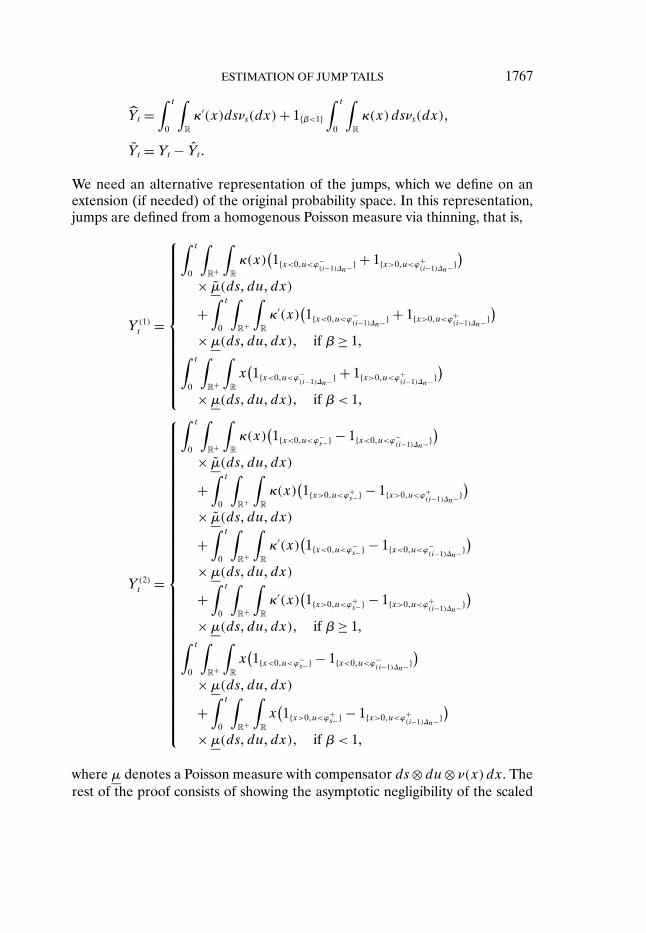
ESTIMATION OF JUMP TAILS 1767
Yt =∫ t
0
∫R
κ′(x)dsνs(dx)+ 1{β<1}
∫ t
0
∫R
κ(x)dsνs(dx)�
Yt = Yt − Yt �
We need an alternative representation of the jumps, which we define on anextension (if needed) of the original probability space. In this representation,jumps are defined from a homogenous Poisson measure via thinning, that is,
Y(1)t =
⎧⎪⎪⎪⎪⎪⎪⎪⎪⎪⎪⎪⎪⎪⎪⎨⎪⎪⎪⎪⎪⎪⎪⎪⎪⎪⎪⎪⎪⎪⎩
∫ t
0
∫R+
∫R
κ(x)(1{x<0�u<ϕ−
(i−1)Δn−} + 1{x>0�u<ϕ+(i−1)Δn−}
)× μ(ds�du�dx)+
∫ t
0
∫R+
∫R
κ′(x)(1{x<0�u<ϕ−
(i−1)Δn−} + 1{x>0�u<ϕ+(i−1)Δn−}
)×μ(ds�du�dx)� if β≥ 1,∫ t
0
∫R+
∫R
x(1{x<0�u<ϕ−
(i−1)Δn−} + 1{x>0�u<ϕ+(i−1)Δn−}
)×μ(ds�du�dx)� if β< 1,
Y(2)t =
⎧⎪⎪⎪⎪⎪⎪⎪⎪⎪⎪⎪⎪⎪⎪⎪⎪⎪⎪⎪⎪⎪⎪⎪⎪⎪⎪⎪⎪⎪⎪⎪⎪⎪⎨⎪⎪⎪⎪⎪⎪⎪⎪⎪⎪⎪⎪⎪⎪⎪⎪⎪⎪⎪⎪⎪⎪⎪⎪⎪⎪⎪⎪⎪⎪⎪⎪⎪⎩
∫ t
0
∫R+
∫R
κ(x)(1{x<0�u<ϕ−
s−} − 1{x<0�u<ϕ−(i−1)Δn−}
)× μ(ds�du�dx)+
∫ t
0
∫R+
∫R
κ(x)(1{x>0�u<ϕ+
s−} − 1{x>0�u<ϕ+(i−1)Δn−}
)× μ(ds�du�dx)+
∫ t
0
∫R+
∫R
κ′(x)(1{x<0�u<ϕ−
s−} − 1{x<0�u<ϕ−(i−1)Δn−}
)×μ(ds�du�dx)+
∫ t
0
∫R+
∫R
κ′(x)(1{x>0�u<ϕ+
s−} − 1{x>0�u<ϕ+(i−1)Δn−}
)×μ(ds�du�dx)� if β≥ 1,∫ t
0
∫R+
∫R
x(1{x<0�u<ϕ−
s−} − 1{x<0�u<ϕ−(i−1)Δn−}
)×μ(ds�du�dx)+
∫ t
0
∫R+
∫R
x(1{x>0�u<ϕ+
s−} − 1{x>0�u<ϕ+(i−1)Δn−}
)×μ(ds�du�dx)� if β< 1,
where μ denotes a Poisson measure with compensator ds⊗ du⊗ ν(x)dx. Therest of the proof consists of showing the asymptotic negligibility of the scaled

1768 T. BOLLERSLEV AND V. TODOROV
sums of the terms aji , j = 1� � � � �7, and their respective subcomponents. We useconvergence in the L1 or L2 norm to prove this.
We begin with the term a1i . Application of Itô ’s lemma yields the decompo-
sition a1i = a1
i + a1i ,
a1i = 2
∫ iΔn
(i−1)Δn
Zns αs ds� a1i = 2
∫ iΔn
(i−1)Δn
Zns σs dWs�
Zns =Zs −Z(i−1)Δn �
We have, for q≥ 1,
E|a1i |q ≤ CΔ3q/2
n �
Also, for q ≥ 2, using Doob’s inequality and the Cauchy–Schwarz inequality,we get
Eni−1a1i = 0�
E|a1i |q ≤ CE
(∫ iΔn
(i−1)Δn
(Zns σs)2 ds
)q/2≤ CΔq/2−1
n
∫ iΔn
(i−1)Δn
E|Zns σs|q ds ≤ CΔqn�
Using Holder’s inequality for any 1 ≤ q < p/2,
E|a2i |q ≤ (E|Δni Z|p)2q/p
(P(|Δni p| ≥ αΔ�n )
)1−2q/p
≤ CΔq+(1−2q/p)(1−βω)−εn � ε > 0�
We proceed with a3i and the decomposition |a3
i | ≤ |a3i | + |a3
i | + |a3i | for
a3i = (Δni Y)21{|Δni Y |≤1�5αΔ�n }� a3
i = (Δni Y)21{|Zni |≥0�25αΔ�n }�
a3i = (Δni Y)21{|Zni |≥0�25αΔ�n }�
Then, for any ε > 0 and q≥ β/2,
E|a3i |q ≤ CΔ(2q−β−ε)�
n E|Δni Y |β+ε ≤ CΔ(2q−β)�+1−εn �
For a3i and p> 2q∨β, we can write
E|a3i |q ≤ CE
(|Δni Y |2q1{|Zni |≥0�25αΔ�n })
≤ C(E|Δni Y |p)2q/p(P(|Zni | ≥ 0�25αΔ�n )
)1−2q/p
≤ CΔ2q/p+(1/2−�)(p−2q)n �

ESTIMATION OF JUMP TAILS 1769
Furthermore, we can bound E|a3i |q ≤ C(E|a3
i (1)|q + E|a3i (2)|q) for
a3i (1)= (
Δni Y(1))2
1{|Zni |≥0�25αΔ�n }� a3i (2)= (
Δni Y(2))2
1{|Zni |≥0�25αΔ�n }�
where Zni is defined on the probability space of Y(1)t , Y(2)
t is the same processon the original probability space, and, for simplicity, we have kept the samenotation. Then, for 1 ≤ q < p/2,
E|a3i (1)|q ≤ E
(Eni−1
∣∣Δni Y (1)∣∣2q
Eni−1
(1{|Zni |≥0�25αΔ�n }
))≤ CΔ1+(1/2−�)(p−2)
n �
Using Holder’s inequality, it follows that for every x > 1,
E|a3i (2)|q ≤ (
E∣∣Δni Y (2)
∣∣2qx)1/x(P(|Zni | ≥ 0�25αΔ�n )
)1−1/x
≤ CΔ(3/2)(1/x)+(1−1/x)(1/2−�)pn �
Next, note that Eni−1a4i = 0 and for 2 ≤ q < p,
E|a4i |q ≤ C(E|Δni Z|p)q/p(E|Δni Y |qp/(p−q))1−q/p
≤ CΔ1+q(1/2−1/p)n �
The a5i term can be decomposed as a5
i = a5i + a5
i ,
a5i = Δn
(C+ϕ+
(i−1)Δn− +C−ϕ−(i−1)Δn−
)Δni Z�
a5i = Δni Z
∫ iΔn
(i−1)Δn
(C+(ϕ+
s −ϕ+(i−1)Δn−
)+C−(ϕ−s −ϕ−
(i−1)Δn−))ds�
where C+ and C− are some constants. Thus for q≥ 2,
Eni−1a5i = 0� E|a5
i |q ≤ CΔ3q/2n �
Application of Holder’s inequality for q≥ 1 and arbitrarily small ε > 0 impliesthat
E|a5i |q ≤ CΔ3q/2+q/2∧1−ε
n �
We turn now to a6i , which can be bounded by |a6
i | ≤ |a6ai | + |a6b
i | + |a6ci |, where
a6ai = 2Zni Δ
ni Y1{|Zni |>0�25αΔ�n }� a6b
i = 2Zni Δni Y1{|Δni Y |>0�5αΔ�n }�
a6ci = 2Zni Δ
ni Y1{|Zni |>0�25αΔ�n }�

1770 T. BOLLERSLEV AND V. TODOROV
For a6ai and p> q∨β, we can apply Holder’s inequality twice, together with the
fact that moments of all powers of the normal distribution exist, to concludethat for some small ε > 0,
E|a6ai |q ≤ C(E|Δni Y |p)q/p
× (E(∣∣σ(i−1)Δn
∣∣qp/(p−q)|Δni W |qp/(p−q)1{|Zni |>0�25αΔ�n }))1−q/p
≤ CΔq/p+q/2n
(E(∣∣σ(i−1)Δn
∣∣(1+ε)qp/(p−q)1{|Zni |>0�25αΔ�n }
))(1−q/p)/(1+ε)
≤ CΔq/p+q/2n
× (E(∣∣σ(i−1)Δn
∣∣(1+ε)qp/(p−q)Pni−1(|Zni |> 0�25αΔ�n )
))(1−q/p)/(1+ε)
≤ CΔq/p+q/2n Δ(1/2−�)(p−q)/(1+ε)
n �
Next, for a6bi , we have E|a6b
i |q ≤ C(E|a6bi (1)|q + E|a6b
i (2)|q + E|a6bi (3)|q), where
a6bi (1)= 2Zni Δ
ni Y
(1)1{|Δni Y (1)|>0�25αΔ�n }�
a6bi (2)= 2Zni Δ
ni Y
(1)1{|Δni Y (2)|>0�25αΔ�n }�
a6bi (3)= 2Zni Δ
ni Y
(2)1{|Δni Y |>0�5αΔ�n }�
Now, Eni−1a6bi (1)= 0 and for some arbitrarily small ε > 0,
E|a6bi (1)|q ≤ CE
(Eni−1|Zni |qEni−1
{∣∣Δni Y (1)∣∣q1{|Δni Y (1)|>0�25αΔ�n }
})≤ CΔ1+q/2−((β−q)∨0)�−ε
n �
For p> q∨β and any ε > 0,
E|a6bi (2)|q ≤ C(E∣∣Zni Δni Y (1)
∣∣p)q/p(E(1{∣∣Δni Y (2)∣∣>0�25αΔ�n }))1−q/p
≤ CΔq/2+q/p+(1−q/p)(3/2−β�)−εn �
By Holder’s inequality for any ε > 0 and q < p,
E|a6bi (3)|q ≤ C(E|Zni |p)q/p
(E∣∣Δni Y (2)
∣∣qp/(p−q))1−q/p
≤ CΔq/2+(3/2)((1/β)∧(p−q)/(pq))q−εn �
Next, note that E|a6ci |q ≤ C(E|a6c
i (1)|q + E|a6ci (2)|q), where
a6ci (1)= 2Zni Δ
ni Y
(1)1{|Zni |>0�25αΔ�n }�
a6ci (2)= 2Zni Δ
ni Y
(2)1{|Zni |>0�25αΔ�n }�

ESTIMATION OF JUMP TAILS 1771
It follows that for q < p,
E|a6ci (1)|q ≤ CE
(Eni−1
(|Zni |q1{|Zni |>0�25αΔ�n })Eni−1
∣∣Δni Y (1)∣∣q)
≤ CΔq/2+(q/β)∧1+(1/2−�)(p−q)n �
For a6ci (2), we can proceed the same way as for a6b
i (3) to show that for anyε > 0 and q < p,
E|a6ci (2)|q ≤ C(E|Zni |p)q/p
(E∣∣Δni Y (2)
∣∣qp/(p−q))1−q/p
≤ CΔq/2+(3/2)((1/β)∧(p−q)/(pq))q−εn �
Using the integrability conditions on αs and σs, and Holder’s inequality, wehave
E|a7i |q ≤ CE
(|Δni ZΔni Y |q1{|Δni Y |≤αΔ�n })
≤ Δq/2+1+(q−β)�∨0−εn � ε > 0� Q.E.D.
LEMMA 2: Suppose we observe the process pt at the discrete times 0�Δn� � � � �nΔn� � � � � t� t+Δn� � � � � t+nΔn� � � � � Assume that A1–A4 hold, and let eitherXt =∫ t+1tσ2s ds or Xt =
∫ t+1t
∫ψ+(x)>�T φ
+i (ψ(x)− �T�θ(1)� θ(2))μ(ds�dx) for i = 1�2
and θ ∈ΘlT . Then for some α > 0 and � ∈ (0� 1
2),
√NT
T
T−1∑t=1
Xt
(TVn
t−1 −∫ t
t−1σ2s ds
)P→ 0 as T ↑ ∞�Δn ↓ 0�(8.10)
provided that√NTΔ
(2−β)�∧1/2−εn → 0 for the deterministic sequence NT ↑ ∞ as
T ↑ ∞ and ε > 0 arbitrarily small.
PROOF: We make the identical decomposition of the difference((Δn�t−1
i p)21{|Δn�t−1i p|≤αΔ�n } −
∫ t−1+iΔn
t−1+(i−1)Δn
σ2s ds
)as in Lemma 1. We denote the corresponding components in this decomposi-tion for the high-frequency interval [t + (i− 1)Δn� t + iΔn] by ajt�i, with each ofthe components denoted analogously. Then using Holder’s inequality for somea > 1,
1T − 1
T−1∑t=1
XtLt ≤(
1T − 1
T−1∑t=1
|Xt |a)1/a(
1T − 1
T−1∑t=1
|Lt |a/(a−1)
)1−1/a
�

1772 T. BOLLERSLEV AND V. TODOROV
where Lt = ∑n
i=1 ajt�i, or the identical sum over their subcomponents. For the
terms involving a1t�i, a
4t�i, a
5t�i, and a6b
t�i(1), we can use a= 2 and show convergenceto zero of NT
T
∑T
t=1 |Lt |2. The latter follows from the bounds on the second mo-ments of a1
t�i, a4t�i, a
5t�i, and a6b
t�i(1) derived in the previous lemma, and the factthat these terms form martingale difference sequences.
For the rest of the terms, we can set set a arbitrarily large. 1T−1
∑T−1t=1 |Xt |a
will be bounded in L1 by the integrability assumptions on the processes σs and
ϕ±s in A4. Asymptotic negligibility of N
0�5a/(a−1)T
T−1
∑T−1t=1 |Lt |a/(a−1) follows from the
basic inequality (∑N
i=1 |ai|)q ≤ Nq−1∑N
i=1 |ai|q for any q > 1 and the boundsderived in the previous lemma for a sufficiently large. Q.E.D.
LEMMA 3: Suppose we observe the process pt at the discrete times 0�Δn�2Δn�� � � � [T/Δn]. Let �T > 1 be a deterministic sequence as a function of the time spanT , such that �T ↑ ∞ as T ↑ ∞. Also, let fT (x) denote a function in x (changingwith T ) with the following properties:
(a) fT (x)= 0 for x < log(�T ).(b) |fT (x)| ≤C(x− log(�T )) and |f ′
T (x)| ≤C for x≥ log(�T ).Let f ′
T (x) denotes the right derivative for x = log(�T ). Then under Assump-tion A1, with ν(x) nondecreasing for x sufficiently large, and Assumption A4,we have
1√NT
([T/Δn]∑i=1
fT (Δni p)−
∑s≤TfT (Δps)
)P→ 0 as T ↑ ∞�Δn ↓ 0(8.11)
for NT = Tν+(log(�T )) and ν+(z)= ∫ ∞zxν(x)dx, provided that for ε > 0 arbi-
trarily small,√NTΔ1−ε
n
(1 ∨
√Δn
ν+(log(�T ))
)→ 0 as T ↑ ∞�Δn ↓ 0�(8.12)
PROOF: For the constant K > 0, denote
pt(K)=∫ t
0αs ds+
∫ t
0σs dWs +
∫ t
0
∫|x|<K
κ(x)μ(ds�dx)
+∫ t
0
∫|x|<K
κ′(x)μ(ds�dx)�
The proof goes through several steps.Step 1. We start by showing that for any s < t and K→ ∞,
P
(sups≤u≤t
ϕ−u + sup
s≤u≤tϕ+u ≥K
)≤ CK−q ∀q > 0�

ESTIMATION OF JUMP TAILS 1773
Using the assumed dynamics for ϕ±u , we can write ϕ±
u − ϕ±s = ∫ u
sα±′v dv +∫ u
sσ±′v dWv + ∫ u
sσ±′′v dBv + ∫ u
s
∫R2 κ(δ
±(v−�x))μ′(ds�dx) + ∫ us
∫R2 κ
′(δ±(v−�x))μ′(ds�dx). The result then follows by using the basic inequality |ϕ±
u | ≤|ϕ±
s | + |ϕ±u − ϕ±
s |, the Burkholder–Davis–Gundy inequality, Chebychev’s in-equality, and, finally, the integrability assumption on the process ϕ±
t .Step 2. We next show that for some constants K0�K1 > 0 and α< 1/β,
P
(∫ iΔn
(i−1)Δn
∫|x|≥K0Δ
αn
μ(ds�dx)≥K1
)≤ CΔ(1−αβ−ε)�K1�
n ∀ε > 0�
We start by introducing the following sets that we rely on later in the proof:
Rn = {x : |x| ≥K0Δαn}� Sn = {x : |x| ≤K0Δ
αn}�
Tn = {x :K0Δαn ≤ |x| ≤K0}�
Using the representation of the jumps with the homogenous measure μ intro-duced in Lemma 1,
P
(∫ iΔn
(i−1)Δn
∫|x|≥K0Δ
αn
μ(ds�dx)≥K1
)
= P
(∫ iΔn
(i−1)Δn
∫R+
∫x∈Rn
(1{x<0�u<ϕ−
s−} + 1{x>0�u<ϕ+s−}
)×μ(ds�du�dx)≥K1
)≤ P
(∫ iΔn
(i−1)Δn
∫R+
∫x∈Rn
1{u<Δ−εn }μ(ds�du�dx)≥K1
)+ P
(sup
s∈[(i−1)Δn�iΔn]ϕ−s ≥ Δ−ε
n
)+ P
(sup
s∈[(i−1)Δn�iΔn]ϕ+s ≥ Δ−ε
n
)�
where ε > 0 is arbitrarily small. For the second probability, we can ap-ply the result of Step 1. For the first probability, we can use the factthat
∫ iΔn(i−1)Δn
∫ Δ−εn
0
∫x∈Rn μ(ds�du�dx) has a Poisson distribution with intensity
Δ1−εn
∫|x|≥K0Δ
αnν(x)dx. Therefore,
P
(∫ iΔn
(i−1)Δn
∫ Δ−εn
0
∫x∈Rn
μ(ds�du�dx)≥K1
)
≤ CΔ(1−ε)�K1�n
(∫|x|≥K0Δ
αn
ν(x)dx
)�K1�
≤ CΔ(1−βα−2ε)�K1�n �

1774 T. BOLLERSLEV AND V. TODOROV
where we made use of the fact that∫
R(|x|β+ς ∧ 1)ν(x)dx <∞ for ς arbitrarily
small.Step 3. We prove
P
(∣∣∣∣∫ iΔn
(i−1)Δn
∫|x|≤K0
κ(x)μ(ds�dx)
+∫ iΔn
(i−1)Δn
∫|x|≤K0
κ′(x)μ(ds�dx)
∣∣∣∣ ≥K1
)≤ CΔ�K1/K0�−ε
n
for ε > 0 sufficiently small. Again, relying on the representation of the jumpsby the homogenous Poisson measure μ on an extended space with the extradimension used for thinning, we have, for Δn sufficiently small (κ′(x) is zerofor |x| in some neighborhood of 0) and 0<α< 1/β,
P
(∣∣∣∣∫ iΔn
(i−1)Δn
∫|x|≤K0
κ(x)μ(ds�dx)
+∫ iΔn
(i−1)Δn
∫|x|≤K0
κ′(x)μ(ds�dx)
∣∣∣∣ ≥K1
)
≤ P
(∣∣∣∣∫ iΔn
(i−1)Δn
∫R+
∫x∈Tn
κ(x)(1{x<0�u<ϕ−
s−} + 1{x>0�u<ϕ+s−}
)× μ(ds�du�dx)
+∫ iΔn
(i−1)Δn
∫R+
∫x∈Tn
κ′(x)(1{x<0�u<ϕ−
s−} + 1{x>0�u<ϕ+s−}
)×μ(ds�du�dx)
∣∣∣∣ ≥ ρK1
)+ P
(∣∣∣∣∫ iΔn
(i−1)Δn
∫R+
∫x∈Sn
κ(x)(1{x<0�u<ϕ−
s−} + 1{x>0�u<ϕ+s−}
)× μ(ds�du�dx)
∣∣∣∣ ≥ (1 − ρ)K1
)for any ρ ∈ (0�1). For the second probability, successive applications ofthe Burkholder–Davis–Gundy inequality and/or the elementary inequality|∑i |ai||p ≤ ∑
i |ai|p for some 0 < p ≤ 1, together with the fact that∫|x|≤K0Δ
αn|κ(x)|qν(x)dx ≤ CΔ(q−β)α−ς
n for q > β and ς > 0 arbitrarily small, im-

ESTIMATION OF JUMP TAILS 1775
ply that for any q > β,
P
(∣∣∣∣∫ iΔn
(i−1)Δn
∫R+
∫x∈Sn
κ(x)(1{x<0�u<ϕ−
s−} + 1{x>0�u<ϕ+s−}
)× μ(ds�du�dx)
∣∣∣∣ ≥ (1 − ρ)K1
)≤ CΔn
∫|x|≤K0Δ
αn
|κ(x)|qν(x)dx+CΔqα+(1−βα)z−ςn
≤ CΔ(q−β)α−ςn � ς > 0
and some z ∈ [0�1). For the first probability, following Step 3, we can split theintegral with respect to the compensated measure into two parts, to concludefor Δn small that
P
(∣∣∣∣∫ iΔn
(i−1)Δn
∫R+
∫x∈Tn
κ(x)(1{x<0�u<ϕ−
s−} + 1{x>0�u<ϕ+s−}
)μ(ds�du�dx)
+∫ iΔn
(i−1)Δn
∫R+
∫x∈Tn
κ′(x)(1{x<0�u<ϕ−
s−} + 1{x>0�u<ϕ+s−}
)×μ(ds�du�dx)
∣∣∣∣ ≥ ρK1
)≤ P
(∣∣∣∣∫ iΔn
(i−1)Δn
∫R+
∫x∈Tn
x(1{x<0�u<ϕ−
s−} + 1{x>0�u<ϕ+s−}
)×μ(ds�du�dx)
∣∣∣∣ ≥ ρK1 −CΔα(1−β−ς)1{β≥1}n
∫ iΔn
(i−1)Δn
(ϕ−s +ϕ+
s ) ds
)
≤ P
(∫ iΔn
(i−1)Δn
∫ Δ−εn
0
∫x∈Tn
|x|μ(ds�du�dx)
≥ ρK1 −CΔ1−α(β−1+ς)1{β≥1}−εn
)+ P
(sup
s∈[(i−1)Δn�iΔn]ϕ−s ≥ Δ−ε
n
)+ P
(sup
s∈[(i−1)Δn�iΔn]ϕ+s ≥ Δ−ε
n
)≤ CP
(∫ iΔn
(i−1)Δn
∫ Δ−εn
0
∫x∈Rn
μ(ds�du�dx)
≥ ρK1 −CΔ1−α(β−1+ς)1{β≥1}−εn
K0
)≤ CΔ(1−αβ−ε)�ρK1/K0�
n �

1776 T. BOLLERSLEV AND V. TODOROV
where ς > 0 is arbitrarily small, and we made use of the results of Steps 1 and 2.The final part of the proof for this step then follows by applying the above twoinequalities with ρ sufficiently close to 1 and α close to 0.
Step 4. Using the integrability assumptions on the processes αt and σt , wehave
P
(∣∣∣∣∫ iΔn
(i−1)Δn
αs ds+∫ iΔn
(i−1)Δn
σs dWs
∣∣∣∣ ≥K1
)≤ CΔqn ∀q > 0�
Step 5. Combining the results of Steps 1–5, it follows that for any �K1/K0�>q,
P(|Δni p(K0)|>K1
) ≤ CΔq−εn ∀ε > 0�
Step 6. For δ ∈ (0�1) with δ > 1/�T , let K > 0 satisfy K < | log(δ)|/3 ∧log(δ�T). Then
E
([T/Δn]∑i=1
∣∣∣∣fT (Δni p)− ∑(i−1)Δn≤s≤iΔn
fT (Δps)
∣∣∣∣1{Ai}
)≤ CTΔ1−ε
n ∀ε > 0�
where Ai = {ω :∫ iΔn(i−1)Δn
∫|x|≥K μ(ds�dx) ≥ 2}. To prove this result, we first use
the fact that
fT (Δni p)≤ C|Δni p|�
E
( ∑(i−1)Δn≤s≤iΔn
|fT (Δps)|)q
≤ CΔnν+(log(�T ))� q≥ 1�
The result of this step then follows readily from Holder’s inequality and theresult of Step 2.
Step 7. For the same choices of δ and K used in Step 6, denote the set Bi ={ω : |Δni p(K)| ≥ | log(δ)|}. Then as in Step 6, using the result of Step 5, we get
E
([T/Δn]∑i=1
∣∣∣∣fT (Δni p)− ∑(i−1)Δn≤s≤iΔn
fT (Δps)
∣∣∣∣1{Aci �Bi}
)≤ CTΔn�
Step 8. Let Ci = {ω :∃s ∈ [(i − 1)Δn� iΔn] :Δps ≥ log(�T )} and Di ={ω :Δni p≥ log(�T )}. We that for some arbitrarily small ε > 0,
E
([T/Δn]∑i=1
∣∣∣∣fT (Δni p)− ∑(i−1)Δn≤s≤iΔn
fT (Δps)
∣∣∣∣1{Aci �Bci �Cci �Di}
)
≤ CΔ1/2−εn T
(ν+(log(�T ))
)1−ε�

ESTIMATION OF JUMP TAILS 1777
On the set Aci ∩Bci ∩Cci ∩Di, there is exactly one jump of size above K in ab-
solute value and its size must be in the interval [log(δ�T)� log(�T )] (recall δ >1/�T ). Therefore, using the fact that |fT (x)− fT (log(�T ))| ≤ C|x− log(�T )|for x≥ log(�T ) and fT (log(�T ))≤ C, we have∣∣∣∣fT (Δni p)− ∑
(i−1)Δn≤s≤iΔnfT (Δps)
∣∣∣∣1{Aci �Bci �Cci �Di}(8.13)
≤ C|Δni p(K)|∫ iΔn
(i−1)Δn
∫R
1{x∈[log(δ�T )�log(�T )]}μ(ds�dx)
+C∫ iΔn
(i−1)Δn
∫R
1(|Δni p(K)| ≥ log(�T )− x�
x ∈ [log(δ�T)� log(�T )])μ(ds�dx)�
Note that in the last integral, the integrand is not adapted, but this does notmatter as the integral with respect to μ is defined in the usual Riemann–Stieltjes sense. Now, using the representation of the jumps with respect to μ,for the first term on the right-hand side of (8.13), we have
E
(|Δni p(K)|
∫ iΔn
(i−1)Δn
∫R
1{x∈[log(δ�T )�log(�T )]}μ(ds�dx))
(8.14)
≤A1 +A2 +A3 +CΔqn�
A1 = E
(∣∣∣∣∫ iΔn
(i−1)Δn
αs ds+∫ iΔn
(i−1)Δn
σs dWs
∣∣∣∣×
∫ iΔn
(i−1)Δn
∫R
1{x∈[log(δ�T )�log(�T )]}μ(ds�dx))�
A2 = E
(∣∣∣∣∫ iΔn
(i−1)Δn
∫R+
∫|x|≤K
κ(x)(1{x<0�u<ϕ−
s−} + 1{x>0�u<ϕ+s−}
)× μ(ds�du�dx)
∣∣∣∣ ∫ iΔn
(i−1)Δn
∫ Δ−εn
0
∫x∈[log(δ�T )�log(�T )]
μ(ds�du�dx))�
A3 = E
(∫ iΔn
(i−1)Δn
∫ Δ−εn
0
∫|x|≤K
|κ′(x)|μ(ds�du�dx)
×∫ iΔn
(i−1)Δn
∫ Δ−εn
0
∫x∈[log(δ�T )�log(�T )]
μ(ds�du�dx)
)for some arbitrarily small ε > 0 and arbitrarily large q > 0. Then for A1, wecan use Holder’s inequality. For A2, we condition first on the filtration gener-
1778 T. BOLLERSLEV AND V. TODOROV
ated byμ(R+�R+�x ∈ [log(δ�T)� log(�T )]) and then apply Burkholder–Davis–Gundy inequality and Holder’s inequality. For A3, we use the independenceof the filtration generated by μ(R+�R+�x ∈ [log(δ�T)� log(�T )]) from that ofμ(R+�R+� |x| ≤K) (note that K < log(δ�T)). Altogether we get, for ρ > 0 ar-bitrarily small,
E
(|Δni p(K)|
∫ iΔn
(i−1)Δn
∫R
1{x∈[log(δ�T )�log(�T )]}μ(ds�dx))
(8.15)
≤ CΔ3/2−ρn ν+(log(δ�T))1−ρ�
Now, for the second term on the right-hand side of (8.13),∫ iΔn
(i−1)Δn
∫R
1(|Δni p(K)| ≥ log(�T )− x�
x ∈ [log(δ�T)� log(�T )])μ(ds�dx)
≤ C|Δni p(K)|1−ρ∫ iΔn
(i−1)Δn
∫R
1| log(�T )− x|1−ρ
× 1(x ∈ [log(δ�T)� log(�T )]
)μ(ds�dx)
for arbitrarily small ρ > 0. From here we can proceed exactly as in (8.15) uponusing, for any 1 ≤ α< 1/(1 − ρ), the bound
E
(∫ iΔn
(i−1)Δn
∫R
1| log(�T )− x|1−ρ 1
(x ∈ [log(δ�T)� log(�T )]
)μ(ds�dx)
)α≤ CΔn
∫x∈[log(δ�T )�log(�T )]
1| log(�T )− x|α(1−ρ) ν(x)dx
+CΔαn(∫
x∈[log(δ�T )�log(�T )]
1| log(�T )− x|1−ρ ν(x)dx
)α≤ CΔnν+(log(δ�T))�
where for the first inequality, we made use of the Burkholder–Davis–Gundyinequality, and for the second, the restriction that α < 1/(1 − ρ) together withthe fact that ν(x) is nonincreasing in the tails.
Step 9. In this step, we show for some arbitrarily small ε > 0 that
E
([T/Δn]∑i=1
∣∣∣∣fT (Δni p)− ∑(i−1)Δn≤s≤iΔn
fT (Δps)
∣∣∣∣1{Aci �Bci �Ci�Dci }
)
≤ CΔ1/2−εn T
(ν+(log(�T ))
)1−ε�

ESTIMATION OF JUMP TAILS 1779
On the set Aci ∩ Bci ∩ Ci ∩ Dc
i , there is exactly one jump of size above K inabsolute value and its size must be in the interval [log(�T )� log(�T )− log(δ)].Then using the fact that |fT (x)| ≤ C for x ∈ [log(�T )� log(�T ) − log(δ)] (Cdepends on δ), we have∣∣∣∣fT (Δni p)− ∑
(i−1)Δn≤s≤iΔnfT (Δps)
∣∣∣∣1{Aci �Bci �Ci�Dci }
≤ C∫ iΔn
(i−1)Δn
∫R
1(|Δni p(K)| ≥ x− log(�T )�
x ∈ [log(�T )� log(�T )− log(δ)])μ(ds�dx)�From here the result follows exactly as in Step 8.
Step 10. In the final step, we show for arbitrarily small ε > 0 that
E
([T/Δn]∑i=1
∣∣∣∣fT (Δni p)− ∑(i−1)Δn≤s≤iΔn
fT (Δps)
∣∣∣∣1{Aci �Bci �Ci�Di}
)
≤ CTΔ1/2−εn
(ν+(log(�T ))
)1−ε�
On the set Aci ∩ Bci ∩ Ci ∩ Di, we have only one jump of p above log(�T ).
Therefore, since the function fT is differentiable for values of the argumentexceeding log(�T ), a first-order Taylor expansion together with the bounded-ness of the first derivative of fT yields∣∣∣∣fT (Δni p)− ∑
(i−1)Δn≤s≤iΔnfT (Δps)
∣∣∣∣1{Aci �Bci �Ci�Di}
≤ C∣∣Δni p(log(�T ))∣∣1{Aci �Bci �Ci�Di}�
To continue further, we introduce the two sets
RT = {x : |x| ≥ log(�T )} and ST = {x : |x| ≤ log(�T )}�Using the alternative representation of the jumps with respect to μ, we have
E
(∣∣∣∣fT (Δni p)− ∑(i−1)Δn≤s≤iΔn
fT (Δps)
∣∣∣∣1{Aci �Bci �Ci�Di}
)
≤ CE
(1{Aci �Bci �Ci�Di}
∣∣Δni p(log(�T ))∣∣
×∫ iΔn
(i−1)Δn
∫u<ϕ+
s−
∫x∈RT
μ(ds�du�dx)
)

1780 T. BOLLERSLEV AND V. TODOROV
≤ CE
(∣∣Δni p(log(�T ))∣∣ ∫ iΔn
(i−1)Δn
∫u<Δ−ε
n
∫x∈RT
μ(ds�du�dx)
)+CE
(∣∣Δni p(log(�T ))∣∣1{sups∈[(i−1)Δn�iΔn] ϕ+
s ≥Δ−εn }
)�
Furthermore,
E
(∣∣Δni p(log(�T ))∣∣ ∫ iΔn
(i−1)Δn
∫u<Δ−ε
n
∫x∈RT
μ(ds�du�dx))
≤ B1 +B2�
where
B1 = CE
[(∫ iΔn
(i−1)Δn
(|αs| +ϕ+s− +ϕ−
s−)ds+∣∣∣∣∫ iΔn
(i−1)Δn
σs dWs
∣∣∣∣)
×∫ iΔn
(i−1)Δn
∫u<Δ−ε
n
∫x∈RT
μ(ds�du�dx)
]�
B2 = CE
[∣∣∣∣∫ iΔn
(i−1)Δn
∫R+
∫x∈ST
x(1{x<0�u<ϕ−
s−} + 1{x>0�u<ϕ+s−}
)× μ(ds�du�dx)
∣∣∣∣×
∫ iΔn
(i−1)Δn
∫u<Δ−ε
n
∫x∈RT
μ(ds�du�dx)]�
By Holder’s inequality and the integrability conditions for some arbitrarilysmall ς > 0,
B1 ≤ CΔ3/2−ςn
(ν+(log(�T ))
)1−ς�
For the term B2, we can condition on the filtration generated by the measureμ(R+�R+�x ∈RT), denoted with F ∗, and use the fact that the Poisson measurecreates independent filtration on disjoint sets (see, e.g., Sato (1999)), to get, byan application of the Burkholder–Davis–Gundy inequality, that
B2 ≤ CE
[√∫ iΔn
(i−1)Δn
E((ϕ+s +ϕ−
s )|F ∗iΔn
∨ F(i−1)Δn) ds
×∫ iΔn
(i−1)Δn
∫u<Δ−ε
n
∫x∈RT
μ(ds�du�dx)
]≤ CΔ1+1/2−2ε
n ν+(log(�T ))+B3�

ESTIMATION OF JUMP TAILS 1781
where
B3 = CE
((E
(∫ iΔn
(i−1)Δn
(ϕ+s +ϕ−
s ) ds
×(∫ iΔn
(i−1)Δn
∫u<Δ−ε
n
∫x∈RT
μ(ds�du�dx)
)2∣∣∣F ∗iΔn
∨ F(i−1)Δn
))1/2
× 1{sups∈[(i−1)Δn�iΔn] ϕ+s ≥Δ−ε
n }
)�
It then follows by the Cauchy–Schwarz inequality that for any q > 0,
B3 ≤ CΔq/2n
(E
(∫ iΔn
(i−1)Δn
(ϕ+s +ϕ−
s ) ds
×(∫ iΔn
(i−1)Δn
∫u<Δ−ε
n
∫x∈RT
μ(ds�du�dx)
)2))1/2
≤ CΔq/2n �
Step 11. Combining the results of Steps 6–10, we get (8.11) provided condi-tion (8.12) holds. Q.E.D.
LEMMA 4: Suppose we observe the process pt at the discrete times 0�Δn� � � � �nΔn� � � � � t� t + Δn� � � � � t + nΔn� � � � and assume that Assumptions A1, with ν(x)nondecreasing for x sufficiently large, and A4 hold. Then, for �T and the functionfT defined in Lemma 3, and provided (8.12) holds, we have
1√NT
T−1∑t=1
(n∑i=1
fT (Δn�ti p)−
t+1∑s=tfT (Δps)
)TVn
t−1(8.16)
P→ 0 as T ↑ ∞�Δn ↓ 0�
PROOF: We can proceed exactly as in the proof of Lemma 2, using the resultin Lemma 3. We only need that E|TVn
t−1|q <∞ for arbitrary q > 0. But thisfollows from an application of Ito’s lemma for the jump increments. Q.E.D.
The proofs of Theorem 3 and Corollary 2 follow from the proof of Theo-rem 1 and Corollary 1 if we can show that
supθ∈ΘlT
√M+T ‖gT (θ��T )− gT (θ��T )‖ P→ 0�

1782 T. BOLLERSLEV AND V. TODOROV
where gT (θ��T ) is defined by substituting∫ t+1t
∫ψ+(x)>�T φ
+i (ψ(x) − �T�θ
(1)�
θ(2))μ(ds�dx) in place of∑n
j=1φ+i (ψ(Δ
n�tj p)−�T�θ(1)� θ(2))1(ψ+(Δn�tj p) > �T)
in gT (θ��T ) for i = 1�2 and t = 0� � � � �T − 1, and in the case of Corollary 1,∫ tt−1σ
2s ds is also replaced by TVn
t for t = 1� � � � � T . But this result follows di-rectly from Lemmas 2 and 4, as the conditions on the function fT are satis-fied by the score functions φ+
i when evaluated at the large jumps on the setθ ∈Θl
T . Q.E.D.
REFERENCES
AÏT-SAHALIA, Y., AND J. JACOD (2009): “Estimating the Degree of Activity of Jumps in HighFrequency Financial Data,” The Annals of Statistics, 37, 2202–2244. [1748]
ANDERSEN, T., T. BOLLERSLEV, AND F. DIEBOLD (2007): “Roughing It Up: Including Jump Com-ponents in the Measurement, Modeling, and Forecasting of Return Volatility,” Review of Eco-nomics and Statistics, 89, 701–720. [1750]
ANDERSEN, T. G., T. BOLLERSLEV, F. X. DIEBOLD, AND P. LABYS (2001): “The Distribution ofRealized Exchange Rate Volatility,” Journal of the American Statistical Association, 96, 42–55.[1752]
BARNDORFF-NIELSEN, O. E., AND N. SHEPHARD (2001): “Non-Gaussian Ornstein–Uhlenbeck-based Models and Some of Their Uses in Financial Economics,” Journal of the Royal StatisticalSociety, Ser. B, 63, 167–241. [1730]
(2004): “Power and Bipower Variation With Stochastic Volatility and Jumps,” Journalof Financial Econometrics, 2, 1–37. [1730,1747,1750]
(2006): “Econometrics of Testing for Jumps in Financial Economics Using BipowerVariation,” Journal of Financial Econometrics, 4, 1–30. [1730,1747,1750]
BARNDORFF-NIELSEN, O. E., P. R. HANSEN, A. LUNDE, AND N. SHEPHARD (2008): “DesigningRealised Kernels to Measure the ex-post Variation of Equity Prices in the Presence of Noise,”Econometrica, 76, 1481–1536. [1752]
BARRO, R. J. (2006): “Rare Disasters and Asset Markets in the Twentieth Century,” QuarterlyJournal of Economics, 121, 823–866. [1757]
BOLLERSLEV, T., AND V. TODOROV (2011a): “Tails, Fears and Risk Premia,” Journal of Finance(forthcoming). [1753,1757]
(2011b): “Supplement to ‘Estimation of Jump Tails’,” Econometrica Supplementary Ma-terial, 79, http://www.econometricsociety.org/ecta/Supmat/9240_data and programs.zip. [1732]
BROADIE, M., M. CHERNOV, AND M. JOHANNES (2009): “Understanding Index Options Re-turns,” Review of Financial Studies, 22, 4493–4529. [1728]
CHERNOV, M., R. GALLANT, E. GHYSELS, AND G. TAUCHEN (2003): “Alternative Models forStock Price Dynamics,” Journal of Econometrics, 116, 225–257. [1749]
DUFFIE, D., J. PAN, AND K. SINGLETON (2000): “Transform Analysis and Asset Pricing for AffineJump-Diffusions,” Econometrica, 68, 1343–1376. [1742]
EMBRECHTS, P., C. KLUPPELBERG, AND T. MIKOSCH (2001): Modelling Extremal Events (ThirdEd.). Berlin: Springer-Verlag. [1735,1737,1749]
GABAIX, X. (2010): “Variable Rare Disasters: An Exactly Solved Framework for Ten Puzzles inMacro-Finance,” Working Paper, New York University. [1757]
GOLDIE, C., AND R. SMITH (1987): “Slow Variation With Remainder: A Survey of the Theoryand Its Applications,” The Quarterly Journal of Mathematics, 38, 45–71. [1735,1758]
HILL, B. (1975): “A Simple General Approach to Inference About the Tail of Distribution,” TheAnnals of Statistics, 12, 1163–1174. [1739]
HUANG, X., AND G. TAUCHEN (2005): “The Relative Contributions of Jumps to Total Variance,”Journal of Financial Econometrics, 3, 456–499. [1750]

ESTIMATION OF JUMP TAILS 1783
JACOD, J. (2008): “Asymptotic Properties of Power Variations and Associated Functionals ofSemimartingales,” Stochastic Processes and Their Applications, 118, 517–559. [1747]
JACOD, J., AND A. N. SHIRYAEV (2003): Limit Theorems for Stochastic Processes (Second Ed.).Berlin: Springer-Verlag. [1761]
JACOD, J., AND V. TODOROV (2010): “Do Price and Volatility Jump Together?” The Annals ofApplied Probability, 20, 1425–1469. [1730,1750,1753]
LEADBETTER, M., AND H. ROOTZEN (1988): “Extremal Theory for Stochastic Processes,” TheAnnals of Probability, 16, 431–478. [1737]
MANCINI, C. (2001): “Disentangling the Jumps of the Diffusion in a Geometric Brownian Mo-tion,” Giornale dell’Istituto Italiano degi Attuari, LXIV, 19–47. [1730,1747]
(2009): “Non-Parametric Threshold Estimation for Models With Stochastic DiffusionCoefficient and Jumps,” Scandinavian Journal of Statistics, 36, 270–296. [1747]
MERTON, R. (1973): “An Intertemporal Capital Asset Pricing Model,” Econometrica, 41, 867–887.[1727]
(1976): “Option Pricing When Underlying Asset Returns Are Discontinuous,” Journalof Financial Economics, 3, 125–144. [1728,1733,1735]
PRAKASA RAO, B. (1988): “Statistical Inference From Sampled Data for Stochastic Processes,”in Contemporary Mathematics, Vol. 80. Providence: Amer. Math. Soc. [1747]
ROSINSKI, J., AND G. SAMORODNITSKY (1993): “Distributions of Subadditive Functionals of Sam-ple Paths of Infinite Divisible Processes,” The Annals of Probability, 21, 996–1014. [1737]
SATO, K. (1999): Lévy Processes and Infinitely Divisible Distributions. Cambridge, U.K.: CambridgeUniversity Press. [1780]
SHIMIZU, Y. (2006): “M-Estimation for Discretely Observed Ergodic Diffusion Processes WithInfinitely Many Jumps,” Statistical Inference for Stochastic Processes, 9, 179–225. [1730]
(2010): “Threshold Selection in Jump-Discriminant Filter for Discretely Observed JumpProcesses,” Statistical Methods and Applications, 19, 355–378. [1747,1750]
SHIMIZU, Y., AND N. YOSHIDA (2006): “Estimation of Parameters for Diffusion Processes WithJumps From Discrete Observations,” Statistical Inference for Stochastic Processes, 9, 227–277.[1730,1747]
SMITH, R. (1987): “Estimating Tails of Probability Distributions,” The Annals of Statistics, 15,1174–1207. [1730,1735,1737,1739,1758]
TODOROV, V. (2009): “Estimation of Coninuous-Time Stochastic Volatility Models With JumpsUsing High-Frequency Data,” Journal of Econometrics, 148, 131–148. [1728]
(2010): “Variance Risk Premia Dynamics: The Role of Jumps,” Review of FinancialStudies, 23, 345–383. [1736]
TODOROV, V., AND G. TAUCHEN (2011): “Volatility Jumps,” Journal of Business & Economic Sta-tistics, 29, 356–371. [1730]
VAN DER VAART, A. (1999): Asymptotic Statistics. Cambridge: Cambridge University Press. [1765]ZHANG, L., P. MYKLAND, AND Y. AÏT-SAHALIA (2005): “A Tale of Two Time Scales: Determin-
ing Integrated Volatility With Noisy High-Frequency Data,” Journal of the American StatisticalAssociation, 100, 1394–1411. [1752]
Dept. of Economics, Duke University, Durham, NC 27708, U.S.A. and NBERand CREATES; [email protected]
andDept. of Finance, Kellogg School of Management, Northwestern University,
Evanston, IL 60208, U.S.A.; [email protected].
Manuscript received April, 2010; final revision received June, 2011.