Atmos. Meas. Tech., 7, 1701–1709, 2014www.atmos-meas-tech.net/7/1701/2014/doi:10.5194/amt-7-1701-2014© Author(s) 2014. CC Attribution 3.0 License.

Estimation of atmospheric mixing layer height from radiosonde dataX. Y. Wang and K. C. Wang

State Key Laboratory of Earth Surface Processes and Resource Ecology, College of Global Change andEarth System Science, Beijing Normal University, Beijing, China

Correspondence to:K. C. Wang (kcwang@bnu.edu.cn)

Received: 6 December 2013 – Published in Atmos. Meas. Tech. Discuss.: 10 February 2014Revised: 14 April 2014 – Accepted: 1 May 2014 – Published: 12 June 2014

Abstract. Mixing layer height (h) is an important parameterfor understanding the transport process in the troposphere, airpollution, weather and climate change. Many methods havebeen proposed to determineh by identifying the turning pointof the radiosonde profile. However, substantial differenceshave been observed in the existing methods (e.g. the potentialtemperature (θ), relative humidity (RH), specific humidity(q) and atmospheric refractivity (N ) methods). These differ-ences are associated with the inconsistency of the tempera-ture and humidity profiles in a boundary layer that is not wellmixed, the changing measurability of the specific humidityand refractivity with height, the measurement error of humid-ity instruments within clouds, and the general existence ofclouds. This study proposes a method to integrate the infor-mation of temperature, humidity and cloud to generate a con-sistent estimate ofh. We apply this method to high verticalresolution (∼ 30 m) radiosonde data that were collected at 79stations over North America during the period from 1998 to2008. The data are obtained from the Stratospheric Processesand their Role in Climate Data Center (SPARC). The resultsshow good agreement with those fromN method as the in-formation of temperature and humidity contained inN ; how-ever, cloud effects that are included in our method increasedthe reliability of our estimatedh. From 1988 to 2008, the cli-matologicalh over North America was 1675± 303 m witha strong east–west gradient: higher values (generally greaterthan 1800 m) occurred over the Midwest US, and lower val-ues (usually less than 1400 m) occurred over Alaska and theUS West Coast.

1 Introduction

The atmospheric boundary layer is the section of the at-mosphere that is sensitive to the varying conditions on theEarth’s surface over a short timescale (hours) (Stull, 1988;Seibert et al., 2000; Sportisse, 2010). During the night, theland surface cools at a faster rate than the atmosphere aboveit because the surface emits more long-wave radiation, whichcauses the temperature to increase with height above the sur-face. This temperature inversion depresses the turbulence be-tween the surface and atmosphere; the resulting stable layeris referred to as the “nocturnal stable boundary layer”. Af-ter sunrise, the surface absorbs solar radiation, and the airabove the surface becomes unstable. Then turbulence (Wanget al., 2007) and the atmospheric boundary layer develop(Stull, 1988). Turbulence is much more efficient than molec-ular conduction at transporting momentum, mass and heat(Wang et al., 2012). Among the turbulent fluxes, the sensibleheat flux transfers the surface-absorbed heat, including so-lar short-wave (Wang et al., 2012) and long-wave radiation(Wang and Dickinson, 2013), to the atmosphere; the latentheat flux moistens the atmosphere. The unstable boundarylayer that occurs during the daytime is also referred to as the“convective boundary layer” or “the mixing layer” becauseit is characterised by strong turbulent motions. An importantfeature of the mixing layer is the transition zone, which ischaracterised by a large variability in pollutants and ambi-ent temperature and humidity values that are between thoseof the well-mixed boundary layer and the stable free tropo-sphere (Seibert et al., 2000; Kim et al., 2007).

Mixing layer height (h) is an important parameter that af-fects the near-surface air pollution concentration because itdetermines the volume in which the emitted pollutants aredispersed (Russell et al., 1974; Menut et al., 1999; Kim et

Published by Copernicus Publications on behalf of the European Geosciences Union.

1702 X. Y. Wang and K. C. Wang: Estimation of atmospheric mixing layer height from radiosonde data

al., 2007; Sportisse, 2010). As air pollution becomes moresevere due to economic development, particularly in devel-oping countries (Wang et al., 2009), knowledge ofh is im-portant to the environmental science community and public.Furthermore,h is related to the warming rate that is causedby the enhanced greenhouse gases (Pielke et al., 2007).

The averageh is located in the middle of the entrainmentlayer where the strongest gradients of the vertical profilesof temperature, humidity and pollutants (Stull, 1988) are lo-cated. These profiles are provided by radio soundings andmany remote sounding systems (Emeis et al., 2008). How-ever, broad application of the remote sensing data has beenhindered by the sharp extinction of the remote sensing sig-nal in high humidity conditions (e.g. cloud or fog) (Ferreroet al., 2010; McGrath-Spangler and Denning, 2012). Manymethods have been proposed to estimateh from the temper-ature and atmospheric composition profiles (Seibert et al.,2000; Basha and Ratnam, 2009; Seidel et al., 2010; Ferrero etal., 2011; Seidel et al., 2012); however, inconsistencies existamong the methods (Seidel et al., 2010; von Engeln and Teix-eira, 2013). Seidel et al. (2010) comparedh values that werederived from the existing methods using radiosonde data andfound substantial differences among the various methods.For example, the RH method systematically overestimatestheh for the presence of clouds or introduces instrument er-rors (Seidel et al., 2010). In this paper, we attempt to ex-plain the nonconformity of various methods and propose amethod to combine all of the individual standards. The pro-posed method is applied to high temporal resolution (6 s) ra-diosonde data available from the Stratospheric Processes andtheir Role in Climate Data Center (SPARC).

The following section provides a brief description of thedata and our methodology. Section 3 presents the results ofthe method at 79 stations over North America during 1998–2008, and the final section provides the conclusions and adiscussion.

2 Data and methods

2.1 Data

High temporal resolution radiosonde data are obtainedfrom the Stratospheric Processes and their Role in ClimateData Center (SPARC) (http://www.sparc.sunysb.edu/html/hres.html) for the period 1998 to 2008. The SPARC dataset consists of historical records at 79 stations over NorthAmerica. This data set includes geopotential height, temper-ature, relative humidity and dew point temperature. Thesevariables are recorded at a 6 s interval, which approximatelycorresponds to a 30 m vertical resolution with a∼ 5 m s−1

vertical velocity of the balloon (Wang and Geller, 2003; Sei-del et al., 2012). Generally, measurements are obtained twicedaily at 00:00 and 12:00 Coordinated Universal Time (UTC).Because this study focuses on mixing layer height, we limit

20

498

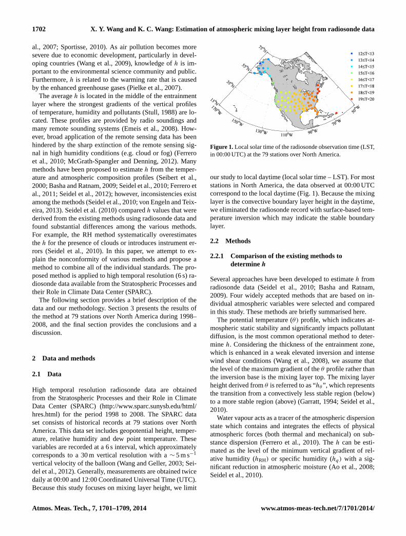
Figure 1. Local solar time of the radiosonde observation time (LST, in 00 UTC) at the 499

79 stations over the North America. 500

Figure 1.Local solar time of the radiosonde observation time (LST,in 00:00 UTC) at the 79 stations over North America.

our study to local daytime (local solar time – LST). For moststations in North America, the data observed at 00:00 UTCcorrespond to the local daytime (Fig. 1). Because the mixinglayer is the convective boundary layer height in the daytime,we eliminated the radiosonde record with surface-based tem-perature inversion which may indicate the stable boundarylayer.

2.2 Methods

2.2.1 Comparison of the existing methods todetermineh

Several approaches have been developed to estimateh fromradiosonde data (Seidel et al., 2010; Basha and Ratnam,2009). Four widely accepted methods that are based on in-dividual atmospheric variables were selected and comparedin this study. These methods are briefly summarised here.

The potential temperature (θ) profile, which indicates at-mospheric static stability and significantly impacts pollutantdiffusion, is the most common operational method to deter-mine h. Considering the thickness of the entrainment zone,which is enhanced in a weak elevated inversion and intensewind shear conditions (Wang et al., 2008), we assume thatthe level of the maximum gradient of theθ profile rather thanthe inversion base is the mixing layer top. The mixing layerheight derived fromθ is referred to as “hθ ”, which representsthe transition from a convectively less stable region (below)to a more stable region (above) (Garratt, 1994; Seidel et al.,2010).

Water vapour acts as a tracer of the atmospheric dispersionstate which contains and integrates the effects of physicalatmospheric forces (both thermal and mechanical) on sub-stance dispersion (Ferrero et al., 2010). Theh can be esti-mated as the level of the minimum vertical gradient of rel-ative humidity (hRH) or specific humidity (hq) with a sig-nificant reduction in atmospheric moisture (Ao et al., 2008;Seidel et al., 2010).

Atmos. Meas. Tech., 7, 1701–1709, 2014 www.atmos-meas-tech.net/7/1701/2014/

X. Y. Wang and K. C. Wang: Estimation of atmospheric mixing layer height from radiosonde data 1703

21

501

Figure 2. The profiles of relative humidity (RH), potential temperature (θ), specific 502

humidity (q), refractivity (N) and the mixing layer height (h) derived from these 503

profiles. The Y-axis is the height above the ground level. h determined by individual 504

standard (magenta dotted line) and h0 which integrates the information of θ, RH, q 505

and N (black solid line) are also shown. (a) Station #14898 at 00 UTC on 13 in 506

August 2006, (b) Station #14898 at 00 UTC on 23 August 2006. (Station #14898: 507

44.5°N, 88.1°W, local solar time: 18:06). 508

509

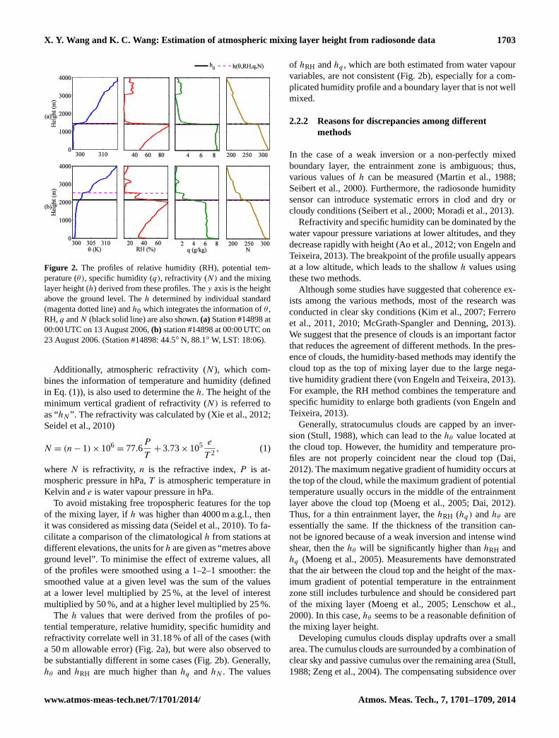
Figure 2. The profiles of relative humidity (RH), potential tem-perature (θ), specific humidity (q), refractivity (N) and the mixinglayer height (h) derived from these profiles. They axis is the heightabove the ground level. Theh determined by individual standard(magenta dotted line) andh0 which integrates the information ofθ ,RH,q andN (black solid line) are also shown.(a) Station #14898 at00:00 UTC on 13 August 2006,(b) station #14898 at 00:00 UTC on23 August 2006. (Station #14898: 44.5◦ N, 88.1◦ W, LST: 18:06).

Additionally, atmospheric refractivity (N ), which com-bines the information of temperature and humidity (definedin Eq. (1)), is also used to determine theh. The height of theminimum vertical gradient of refractivity (N) is referred toas “hN ”. The refractivity was calculated by (Xie et al., 2012;Seidel et al., 2010)

N = (n − 1) × 106= 77.6

P

T+ 3.73× 105 e

T 2, (1)

whereN is refractivity, n is the refractive index,P is at-mospheric pressure in hPa,T is atmospheric temperature inKelvin ande is water vapour pressure in hPa.

To avoid mistaking free tropospheric features for the topof the mixing layer, ifh was higher than 4000 m a.g.l., thenit was considered as missing data (Seidel et al., 2010). To fa-cilitate a comparison of the climatologicalh from stations atdifferent elevations, the units forh are given as “metres aboveground level”. To minimise the effect of extreme values, allof the profiles were smoothed using a 1–2–1 smoother: thesmoothed value at a given level was the sum of the valuesat a lower level multiplied by 25 %, at the level of interestmultiplied by 50 %, and at a higher level multiplied by 25 %.

The h values that were derived from the profiles of po-tential temperature, relative humidity, specific humidity andrefractivity correlate well in 31.18 % of all of the cases (witha 50 m allowable error) (Fig. 2a), but were also observed tobe substantially different in some cases (Fig. 2b). Generally,hθ and hRH are much higher thanhq and hN . The values

of hRH andhq , which are both estimated from water vapourvariables, are not consistent (Fig. 2b), especially for a com-plicated humidity profile and a boundary layer that is not wellmixed.

2.2.2 Reasons for discrepancies among differentmethods

In the case of a weak inversion or a non-perfectly mixedboundary layer, the entrainment zone is ambiguous; thus,various values ofh can be measured (Martin et al., 1988;Seibert et al., 2000). Furthermore, the radiosonde humiditysensor can introduce systematic errors in clod and dry orcloudy conditions (Seibert et al., 2000; Moradi et al., 2013).

Refractivity and specific humidity can be dominated by thewater vapour pressure variations at lower altitudes, and theydecrease rapidly with height (Ao et al., 2012; von Engeln andTeixeira, 2013). The breakpoint of the profile usually appearsat a low altitude, which leads to the shallowh values usingthese two methods.

Although some studies have suggested that coherence ex-ists among the various methods, most of the research wasconducted in clear sky conditions (Kim et al., 2007; Ferreroet al., 2011, 2010; McGrath-Spangler and Denning, 2013).We suggest that the presence of clouds is an important factorthat reduces the agreement of different methods. In the pres-ence of clouds, the humidity-based methods may identify thecloud top as the top of mixing layer due to the large nega-tive humidity gradient there (von Engeln and Teixeira, 2013).For example, the RH method combines the temperature andspecific humidity to enlarge both gradients (von Engeln andTeixeira, 2013).

Generally, stratocumulus clouds are capped by an inver-sion (Stull, 1988), which can lead to thehθ value located atthe cloud top. However, the humidity and temperature pro-files are not properly coincident near the cloud top (Dai,2012). The maximum negative gradient of humidity occurs atthe top of the cloud, while the maximum gradient of potentialtemperature usually occurs in the middle of the entrainmentlayer above the cloud top (Moeng et al., 2005; Dai, 2012).Thus, for a thin entrainment layer, thehRH (hq) andhθ areessentially the same. If the thickness of the transition can-not be ignored because of a weak inversion and intense windshear, then thehθ will be significantly higher thanhRH andhq (Moeng et al., 2005). Measurements have demonstratedthat the air between the cloud top and the height of the max-imum gradient of potential temperature in the entrainmentzone still includes turbulence and should be considered partof the mixing layer (Moeng et al., 2005; Lenschow et al.,2000). In this case,hθ seems to be a reasonable definition ofthe mixing layer height.

Developing cumulus clouds display updrafts over a smallarea. The cumulus clouds are surrounded by a combination ofclear sky and passive cumulus over the remaining area (Stull,1988; Zeng et al., 2004). The compensating subsidence over

www.atmos-meas-tech.net/7/1701/2014/ Atmos. Meas. Tech., 7, 1701–1709, 2014

1704 X. Y. Wang and K. C. Wang: Estimation of atmospheric mixing layer height from radiosonde data

this area effectively produces a stable layer close to the cloudbase (Zeng et al., 2004). Additionally, latent heat releasedin the cloud (Tjernström, 2007) can lead to a weak inver-sion in the cloud. The stable layer within the cloud can actas a turbulence barrier to the air pollution and inhibit tur-bulence under the stable layer. Nonetheless, clouds can alsoencourage pollutant dispersion and enhance mixing due tothe cloud-venting (Cotton et al., 1995; Verzijlbergh et al.,2009). The vertical motion of pollutants mainly depends onthe atmospheric stability in the cloud. In a stable stratifica-tion, air parcels are either neutrally or negatively buoyant,which reduces the buoyancy of the thermals beneath thislayer through vertical mixing. In the case of a thick elevatedstable stratification, the maximum vertical gradient of poten-tial temperature regarded ash instead of cloud top, where asharp reduction of moisture occurs (i.e.hRH or hq ). For deepconvective clouds, updrafts in the cloud are strong enough totransport the air in the mixing layer to the upper free atmo-sphere. Theh should be defined as the cloud base to avoidmistaking the top of the troposphere as the top of the mixinglayer (Stull, 1988). In our study, the mixing layer is limited to4000 m, which may exclude cases of deep convective cloudsin the boundary layer.

2.2.3 A reliable method to produce consistent estimatesof mixing layer height (hcon)

Although all four of the variables can introduce uncertaintiesinto theh estimation, the temperature and humidity factorsare the most important for producing a superiorh estimation:the temperature quantifies the inversion and the water vapourdescribes the mixing capability. In this section, we proposean integrated method that contains the information of tem-perature and moisture, and provides a reasonable definitionof a cloud-capped mixing layer height.

For a non-perfectly mixed boundary layer, the method maynot simultaneously satisfy the criteria that all four individualvariables have the highest vertical gradients at the same level.Instead, we identify the height where the criteria are best metand label ith0. In other words, all of the variables exhibitsharp variations at the selected height (h0), but not necessar-ily the sharpest variations of the entire profiles.

For stratocumulus and stratus capped boundary layers, in-versions are located near the cloud top, whereas for somecumulus, the stable layer usually occurs near the cloud base(Zeng et al., 2004). The level with the greatest potential tem-perature gradient in the stable layer near the cloud ishcon (seeSect. 2.2.1). Considering that the average distance betweenthe cloud top and the level of the largest potential tempera-ture gradient in the entrainment zone is approximately 20 m(Moeng et al., 2005), we scan 90 m (∼ 3 levels with the 30 mvertical resolution radiosonde data) upward from the cloudtop to identify any inversions. Likewise, we search three lev-els downward and upward of the cloud to ensure the exis-tence of a stable layer. If a stable layer cannot be identified

near the cloud, then theh0 is set ashcon; thus, cloud is as-sumed to enhance the mixing.

Clouds are derived from the radiosonde data set by ref-erencing the relative humidity to a specific threshold, basedon the method proposed by Wang and Poore (Poore et al.,1995). The method was later modified by Zhang (Zhang etal., 2010) and validated by independent observations (Zhanget al., 2013).

Following the above qualitative guidelines, an objectiveapproach is proposed based on our radiosonde data.

1. Identify the height (h0) that best meets the four individ-ual criteria:

a. Smooth the gradient profiles ofθ , RH, q andN by1–2–1 smoother.

b. Locate the altitudes of the 10 smallest gradients (orlargest forθ ) of the four variables. All 10 altitudesare considered to meet the criterion of the mixinglayer top and are likely to be theh.

c. Starting with the altitudes of the smallest gradients(or largest forθ), identify the first altitude whereat least three of the four variables meet the crite-ria of h simultaneously. The altitude meeting thesecriteria is set ash0. The allowable error is 50 m. Ifall altitudes do not meet the criteria until the 10thsmallest gradient, then the mixing layer height forthe specific record is missing.

2. Derive the location of the cloud (Zhang et al., 2010):

a. Transform the RH with respect to ice instead of liq-uid water for all of the levels with temperatures be-low 0◦C.

b. Derive the boundary of the moist layer. The base ofthe moist layer is defined as the level where the RHexceeds the min-RH corresponding to this level.Likewise, the top of the moist layer is determinedas the level where the RH decreases to the min-RH corresponding to the level or where the top ofthe profile is reached. Any moist layer with a baselower than 120 m was discarded. The min-RH valueis specified in Table 1.

c. The moist layer is classified as a cloud layer ifthe maximum RH within this layer is greater thanthe corresponding max-RH at the base of the moistlayer. Two contiguous layers are considered a one-layer cloud if the distance between the two layersis less than 300 m or if the minimum RH over thedistance is larger than the maximum inter-RH valuewithin this distance. The max-RH, inter-RH valuesare specified in Table 1.

Atmos. Meas. Tech., 7, 1701–1709, 2014 www.atmos-meas-tech.net/7/1701/2014/

X. Y. Wang and K. C. Wang: Estimation of atmospheric mixing layer height from radiosonde data 1705

Table 1.Summary of height-resolving RH thresholds for cloud de-tection.

Altitude range min-RH (%) max-RH (%) inter-RH (%)

0–2 km 92–90 95–93 84–822–6 km 90–88 93–90 80–786–12 km 88–75 90–80 78–70> 12 km 75 80 70

3. Determine a consistent mixing layer height (hcon):

a. If the h0 is lower than the base of the lowest cloudor identified in clear sky conditions, then thehconequalsh0.

b. If the h0 is higher than the base of the lowest cloud,then scan from the lower three levels of the cloudbase to the upper three levels of the cloud top toidentify the first stable layer that is deeper than100 m. Set the level of the sharpest inversion in thestable layer ashcon. If a stable layer does not existwithin the cloud, then thehcon equalsh0.

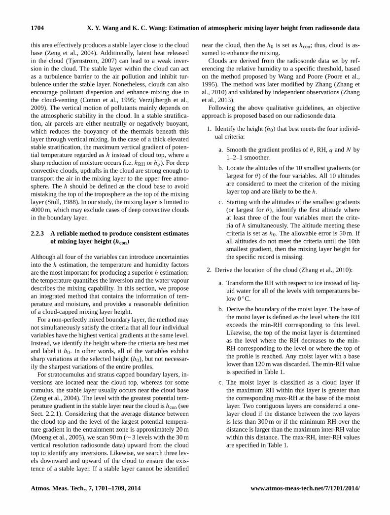
Figure 3 displays three cases in which the boundary layerclouds affect the development of turbulence. When an inver-sion caps the top of the cloud (Fig. 3a) or is located near thecloud base (Fig. 3b), then the level of the sharpest inversionis assigned as the mixing layer height. In this case, the inver-sion near the cloud inhibits the diffusion of pollutants. In thescenario depicted in Fig. 3c, a stable layer is not identified,the cloud accelerates the diffusion and thehcon is consideredas theh0.

3 Results

Section 2 describes a method to integrate existing standardsto produce a consistent estimate of mixing layer height. Thestatistical properties of the estimate and a comparison withthe existing methods are discussed in this section. Addition-ally, the North American mixing layer height climatology ispresented.

3.1 Statistical properties of the mixing layer height(hcon) estimates

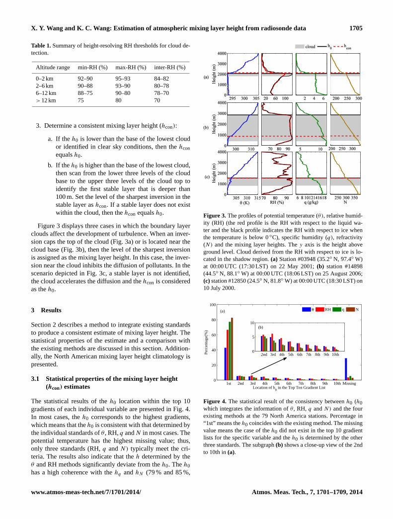
The statistical results of theh0 location within the top 10gradients of each individual variable are presented in Fig. 4.In most cases, theh0 corresponds to the highest gradients,which means that theh0 is consistent with that determined bythe individual standards ofθ , RH,q andN in most cases. Thepotential temperature has the highest missing value; thus,only three standards (RH,q andN) typically meet the cri-teria. The results also indicate that theh determined by theθ and RH methods significantly deviate from theh0. Theh0has a high coherence with thehq andhN (79 % and 85 %,

22

510

Figure 3. The profiles of potential temperature (θ), relative humidity (RH) (red line is 511

the RH respected to the water and black line indicates the RH respected to ice when 512

the temperature below 0°C), specific humidity (q), refractivity (N) and the mixing 513

layer heights. The Y-axis is the height above the ground level. Cloud derived from the 514

RH respected to ice is located at the shadow region. (a) Station #03948 (35.2°N, 515

97.4°W) at 00 UTC (17:30 LST) on 22 May 2001; (b) Station #14898 (44.5°N, 516

88.1°W) at 00 UTC (18:06 LST) on 25 August 2006; (c) Station #12850 (24.5°N, 517

81.8°W) at 00 UTC (18:30 LST) on 10 July 2000. 518

Figure 3. The profiles of potential temperature (θ), relative humid-ity (RH) (the red profile is the RH with respect to the liquid wa-ter and the black profile indicates the RH with respect to ice whenthe temperature is below 0◦C), specific humidity (q), refractivity(N) and the mixing layer heights. They axis is the height aboveground level. Cloud derived from the RH with respect to ice is lo-cated in the shadow region.(a) Station #03948 (35.2◦ N, 97.4◦ W)at 00:00 UTC (17:30 LST) on 22 May 2001;(b) station #14898(44.5◦ N, 88.1◦ W) at 00:00 UTC (18:06 LST) on 25 August 2006;(c) station #12850 (24.5◦ N, 81.8◦ W) at 00:00 UTC (18:30 LST) on10 July 2000.

1st 2nd 3rd 4th 5th 6th 7th 8th 9th 10th Missing0

20

40

60

80

100

Location of h0 in the Top Ten Gradient List

Perc

enta

ge(%

)

θ RH q N

2nd 3rd 4th 5th 6th 7th 8th 9th 10th0

5

10

(a)

(b)

Figure 4. The statistical result of the consistency betweenh0 (h0which integrates the information ofθ , RH, q andN) and the fourexisting methods at the 79 North America stations. Percentage in“1st” means theh0 coincides with the existing method. The missingvalue means the case of theh0 did not exist in the top 10 gradientlists for the specific variable and theh0 is determined by the otherthree standards. The subgraph(b) shows a close-up view of the 2ndto 10th in(a).

www.atmos-meas-tech.net/7/1701/2014/ Atmos. Meas. Tech., 7, 1701–1709, 2014

1706 X. Y. Wang and K. C. Wang: Estimation of atmospheric mixing layer height from radiosonde data

24

526

Figure 5. The frequency histogram of the effect of cloud on pollutants diffusion. The 527

“clear sky” indicates there is no cloud in the boundary layer, otherwise, boundary 528

layer is cloud-taped; “cloud-enhance” means clouds stimulate turbulence in the 529

cloud-capped conditions; “cloud-inhibit” indicates the case that the inversion in the 530

cloud suppresses turbulence in the cloud-capped conditions. The stations are sorted by 531

the value of clear sky percentage. 532

Figure 5. Frequency histogram of the effect of cloud on pollu-tants diffusion. The “clear sky” indicates that there is no cloud inthe boundary layer; otherwise, the boundary layer is cloud-taped.The “cloud-enhance” means that clouds stimulate turbulence in thecloud-capped conditions. The “cloud-inhibit” indicates the case thatthe inversion in the cloud suppresses turbulence in the cloud-cappedconditions. The stations are sorted by the value of clear sky percent-age.

Table 2. A summary of the comparison of thehcon with hθ , hRH,hq , hN andh0, including correlation coefficient, bias and standarddeviation.hcon is the final consistent estimate ofh which includethe information of temperature, water vapour and cloud;hθ , hRH,hq , hN are theh derived from the individual standard of potentialtemperature (θ), relative humidity (RH), specific humidity (q) andatmospheric refractivity (N) respectively;h0 indicates theh inte-grating the information ofθ , RH, q andN which is a transition tothehcon.

Methodhcon

hθ hRH hq hN h0

Correlation coefficient 0.86 0.90 0.96 0.97 0.98Bias (m) 506.2 522.9 116.2 −22.9 37.6Standard deviation (m) 161.5 131.1 71.4 74.8 25.1

respectively) and a relatively low coherence with thehθ andhRH (44 % and 68 %, respectively).

Figure 5 displays the percentage of theh0 values that areinfluenced by clouds at the 79 stations: 72.3 % of the mix-ing layer has clear sky conditions (no clouds in the lowest4000 m above the surface) and 27.7 % of the mixing layeris cloud-capped. In the cloud-capped scenarios, the cloudsstimulate turbulence for approximate one-third of the cloudycases. For the other two-thirds of the cases, inversions nearthe clouds suppress turbulence; therefore, the level of thesharpest inversion is the mixing layer height. However, theN

method never defines cloud base ash because of the higherrefractivity in clouds than beneath clear air.

3.2 Comparison ofhcon with other methods

To reduce the impact of missing data, we calculated themonthly h only if the daily h is available for more than15 days during a month. The annualh is only calculated

25

533

Figure 6. The comparison of the climatological hcon with hθ (blue), hRH (red), hq 534

(green), hN (brown) and h0 (black) for the period of 1998 to 2008. 535

Figure 6. Comparison of the climatologicalhcon with hθ (blue),hRH (red), hq (green),hN (brown) andh0 (black) for the period1998–2008.

if the monthly values are available for more than 6 monthsduring a year. The climatologicalh values for 57 of the 79stations that meet these requirements are shown in Fig. 6and summarised in Table 2. The averages of thehcon andh0are 1675 m and 1713 m, respectively; thus, theh decreasesby 38 m when considering the cloud impacts on turbulence.The values of thehRH andhθ have much higher mean values(2199 m and 2182 m, respectively) and lower coherence withthe hcon. The climatologies of thehq andhN are relativelylower: 1792 m and 1653 m, respectively. The value of thehN

has the best agreement withhcon, which may be due to the in-formation of temperature and water vapour contained in therefractivity concurrently. However, the contribution of watervapour to the refractivity may be higher than that of tempera-ture in the lower troposphere (Basha and Ratnam, 2009); theN method cannot account for the effect of clouds. Further-more, the temperature variable can derive the vertical struc-ture of the cloud. Therefore, the temperature and moisture in-formation provided by the radiosonde can be a vital resourceto estimate the mixing layer height.

3.3 Climatology of mixing layer height overNorth America

Figure 7 displays the multi-year average of thehcon patternover North America. A strong east–westh gradient wherethe higherh over the western states is consistent with thespatial distribution of theh derived from the Cloud-AerosolLidar with Orthogonal Polarization (CALIOP) data set of theCALIPSO satellite (McGrath-Spangler and Denning, 2012,2013). The climatologicalh over the Midwest US is gen-erally greater than 1800 m, whereas the values are usuallyless than 1400 m over Alaska and the US West Coast due

Atmos. Meas. Tech., 7, 1701–1709, 2014 www.atmos-meas-tech.net/7/1701/2014/

X. Y. Wang and K. C. Wang: Estimation of atmospheric mixing layer height from radiosonde data 1707

26

536

Figure 7. Pattern of climatological hcon over North America during the period of 1998 537

to 2008 (unit: meter). All the 57 stations showed here are the stations who meet the 538

long-term average criteria mentioned at the beginning of Sect 3.1. 539

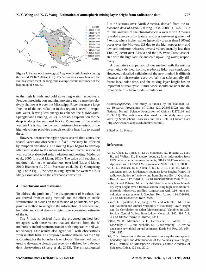
Figure 7.Pattern of climatologicalhcon over North America duringthe period 1998–2008 (unit: m). The 57 stations shown here are thestations which meet the long-term average criteria mentioned at thebeginning of Sect. 3.1.

to the high latitude and cold upwelling water, respectively.Frequent precipitation and high moisture may cause the rela-tively shallowerh over the Mississippi River because a largefraction of the net radiation in this region is used to evapo-rate water, leaving less energy to enhance theh (McGrath-Spangler and Denning, 2012). A possible explanation for thedeeph along the semiarid Rocky Mountains in the south-western US is that the low soil moisture characteristic of thehigh elevations provides enough sensible heat flux to extendtheh.

However, because the region spans several time zones, thespatial variations observed at a fixed time may be affectedby temporal variations. The mixing layer begins to developafter sunrise due to the increased turbulent fluxes associatedwith surface-absorbed solar radiation and heating (Medeiroset al., 2005; Liu and Liang, 2010). The value ofh reaches itsmaximum during the late afternoon over land (Liu and Liang,2010; Bianco et al., 2011; Svensson et al., 2011). ComparingFig. 7 with Fig. 1, the deep mixing layer in the western US islikely associated with the afternoon convection.

4 Conclusions and discussion

To address the problem of the disagreement ofh values thatare derived from existing methods and the effect of stablestratification in clouds on the diffusion of pollutants, we pro-posed a method to integrate the information of temperature,humidity and cloud effects to determine a consistent estimateof theh.

The h that is derived from the proposed method bet-ter agrees with those values that are derived from theN

method (N includes information of both temperature and wa-ter vapour). Our results also agree well with observationsfrom satellite lidar. The proposed method determines theh byaccounting for the boundary layer clouds. The method that isused to determine clouds was recently validated by indepen-dent observations (Zhang et al., 2013). The climatological

h at 57 stations over North America, derived from the ra-diosonde data of SPARC during 1998–2008, is 1675± 303m. The analysis of the climatologicalh over North Americarevealed a noteworthy feature: a strong east–west gradient ofh exists, where higher values (generally greater than 1800 m)occur over the Midwest US due to the high topography andlow soil moisture, whereas lowerh values (usually less than1400 m) occur over Alaska and the US West Coast, associ-ated with the high latitude and cold upwelling water, respec-tively.

A qualitative comparison of our method with the mixinglayer height derived from space-borne lidar was conducted.However, a detailed validation of the new method is difficultbecause the observations are available at substantially dif-ferent local solar time, and the mixing layer height has animportant diurnal cycle. Future work should consider the di-urnal cycle ofh from model simulations.

Acknowledgements.This study is funded by the National Ba-sic Research Programme of China (2012CB955302) and theNational Natural Science Foundation of China (41175126 and91337111). The radiosonde data used in this study were pro-vided by Stratospheric Processes and their Role in Climate Data(http://www.sparc.sunysb.edu/html/hres.html).

Edited by: L. Bianco

References

Ao, C., Chan, T., Iijima, B., Li, J., Mannucci, A., Teixeira, J., Tian,B., and Waliser, D.: Planetary boundary layer information fromGPS radio occultation measurements, GRAS SAF Workshop onApplications of GPSRO Measurements, 2008, 123–131, 2008.

Ao, C. O., Waliser, D. E., Chan, S. K., Li, J. L., Tian, B., Xie, F.,and Mannucci, A. J.: Planetary boundary layer heights from GPSradio occultation refractivity and humidity profiles, J. Geophys.Res.-Atoms., 117, D16117, doi:10.1029/2012JD017598, 2012.

Basha, G. and Ratnam, M. V.: Identification of atmospheric bound-ary layer height over a tropical station using high–resolution ra-diosonde refractivity profiles: Comparison with GPS radio oc-cultation measurements, J. Geophys. Res.-Atmos., 114, D16101,doi:10.1029/2008JD011692, 2009.

Bianco, L., Djalalova, I. V., King, C. W., and Wilczak, J. M.: Diur-nal Evolution and Annual Variability of Boundary-Layer Heightand Its Correlation to Other Meteorological Variables in Cali-fornia’s Central Valley, Bound.-Lay. Meteorol., 140, 491–511,doi:10.1007/s10546-011-9622-4, 2011.

Cotton, W. R., Alexander, G. D., Hertenstein, R., Walko, R. L.,McAnelly, R. L., and Nicholls, M.: Cloud venting – A reviewand some new global annual estimates, Earth-Sci. Rev., 39, 169–206, 1995.

Dai, C. Y.: Properties of the entrainment zone atop the atmosphericboundary layer and determination of the boundary layer height,Ph.D, Institute of Atmospheric Physics, Chinese Academy ofSciences, China, 129 pp., 2012.

www.atmos-meas-tech.net/7/1701/2014/ Atmos. Meas. Tech., 7, 1701–1709, 2014

1708 X. Y. Wang and K. C. Wang: Estimation of atmospheric mixing layer height from radiosonde data

Emeis, S., Schaefer, K., and Muenkel, C.: Surface-based remotesensing of the mixing-layer height-a review, Meteorol. Z., 17,621–630, doi:10.1127/0941-2948/2008/0312, 2008.

Ferrero, L., Perrone, M. G., Petraccone, S., Sangiorgi, G., Ferrini,B. S., Lo Porto, C., Lazzati, Z., Cocchi, D., Bruno, F., Greco,F., Riccio, A., and Bolzacchini, E.: Vertically-resolved particlesize distribution within and above the mixing layer over theMilan metropolitan area, Atmos. Chem. Phys., 10, 3915–3932,doi:10.5194/acp-10-3915-2010, 2010.

Ferrero, L., Riccio, A., Perrone, M., Sangiorgi, G., Ferrini, B.,and Bolzacchini, E.: Mixing height determination by tetheredballoon-based particle soundings and modeling simulations, At-mos. Res., 102, 145–156, 10.1016/j.atmosres.2011.06.016, 2011.

Garratt, J. R.: The atmospheric boundary layer, Cambridge univer-sity press, 1994.

Kim, S.-W., Yoon, S.-C., Won, J.-G., and Choi, S.-C.: Ground-basedremote sensing measurements of aerosol and ozone in an urbanarea: A case study of mixing height evolution and its effect onground-level ozone concentrations, Atmos. Environ, 41, 7069–7081, doi:10.1016/j.atmosenv.2007.04.063, 2007.

Lenschow, D. H., Zhou, M., Zeng, X., Chen, L., and Xu,X.: Measurements of fine-scale structure at the top ofmarine stratocumulus, Bound-Lay. Meteorol., 97, 331–357,doi:10.1023/A:1002780019748, 2000.

Liu, S. and Liang, X.-Z.: Observed Diurnal Cycle Climatology ofPlanetary Boundary Layer Height, J. Climate, 23, 5790–5809,doi:10.1175/2010jcli3552.1, 2010.

Martin, C. L., Fitzjarrald, D., Garstang, M., Oliveira, A. P., Greco,S., and Browell, E.: Structure and growth of the mixing layer overthe Amazonian rain forest, J. Geophys. Res-Atmos., 93, 1361–1375, doi:10.1029/JD093iD02p01361, 1988.

McGrath-Spangler, E. L. and Denning, A. S.: Estimates of NorthAmerican summertime planetary boundary layer depths derivedfrom space-borne lidar, J. Geophys. Res-Atmos., 117, D15101,doi:10.1029/2012JD017615, 2012.

McGrath-Spangler, E. L. and Denning, A. S.: Global seasonal vari-ations of midday planetary boundary layer depth from CALIPSOspace-borne LIDAR, J. Geophys. Res-Atmos., 118, 1226–1233,doi:10.1002/jgrd.50198, 2013.

Medeiros, B., Hall, A., and Stevens, B.: What controls themean depth of the PBL?, J. Climate, 18, 3157–3172,doi:10.1175/jcli3417.1, 2005.

Menut, L., Flamant, C., Pelon, J., and Flamant, P. H.: Ur-ban boundary-layer height determination from lidar mea-surements over the Paris area, Appl. Optics, 38, 945–954,doi:10.1364/AO.38.000945, 1999.

Moeng, C., Stevens, B., and Sullivan, P.: Where is the interface ofthe stratocumulus-topped PBL?, J. Atmos. Sci., 62, 2626–2631,doi:10.1175/JAS3470.1, 2005.

Moradi, I., Soden, B., Ferraro, R., Arkin, P., and Vömel, H.: As-sessing the quality of humidity measurements from global oper-ational radiosonde sensors, J. Geophys. Res-Atmos., 118, 8040–8053, doi:10.1002/jgrd.50589, 2013.

Pielke, R. A., Davey, C. A., Niyogi, D., Fall, S., Steinweg-Woods,J., Hubbard, K., Lin, X., Cai, M., Lim, Y. K., and Li, H.:Unresolved issues with the assessment of multidecadal globalland surface temperature trends, J. Geophys. Res., 112, D16113,doi:10.1029/2006JD008229, 2007.

Poore, K. D., Junhong, W., and Rossow, W. B.: Cloud layer thick-nesses from a combination of surface and upper-air observations,J. Climate, 8, 550–568, 1995.

Russell, P. B., Uthe, E. E., Ludwig, F. L., and Shaw, N. A.: Acomparison of atmospheric structure as observed with monos-tatic acoustic sounder and lidar techniques, J. Geophys. Res., 79,5555–5566, doi:10.1029/JC079i036p05555, 1974.

Seibert, P., Beyrich, F., Gryning, S.-E., Joffre, S., Rasmussen, A.,and Tercier, P.: Review and intercomparison of operational meth-ods for the determination of the mixing height, Atmos. Environ,34, 1001–1027, doi:10.s1352-2310(99)00349-0, 2000.

Seidel, D. J., Ao, C. O., and Li, K.: Estimating climatological plane-tary boundary layer heights from radiosonde observations: Com-parison of methods and uncertainty analysis, J. Geophys. Res.,115, D16113, doi:10.1029/2009JD013680, 2010.

Seidel, D. J., Zhang, Y., Beljaars, A., Golaz, J. C., Jacobson, A. R.,and Medeiros, B.: Climatology of the planetary boundary layerover the continental United States and Europe, J. Geophys. Res.,117, D17106, doi:10.1029/2012JD018143, 2012.

Sportisse, B.: Fundamentals in air pollution: from processes to mod-elling, Atmospheric Boundary Layer, Springer, 93–132, 2010.

Stull, R. B.: An introduction to boundary layer meteorology, Kluweracademic publishers, 665 pp., 1988.

Svensson, G., Holtslag, A. A. M., Kumar, V., Mauritsen, T., Steen-eveld, G. J., Angevine, W. M., Bazile, E., Beljaars, A., de Bruijn,E. I. F., Cheng, A., Conangla, L., Cuxart, J., Ek, M., Falk, M.J., Freedman, F., Kitagawa, H., Larson, V. E., Lock, A., Mail-hot, J., Masson, V., Park, S., Pleim, J., Soderberg, S., Weng, W.,and Zampieri, M.: Evaluation of the Diurnal Cycle in the Atmo-spheric Boundary Layer Over Land as Represented by a Vari-ety of Single-Column Models: The Second GABLS Experiment,Bound.-Lay. Meteorol., 140, 177–206, doi:10.1007/s10546-011-9611-7, 2011.

Tjernström, M.: Is There a Diurnal Cycle in the Summer Cloud-Capped Arctic Boundary Layer?, J. Atmos. Sci., 64, 3970–3986,doi:10.1175/2007JAS2257.1, 2007.

Verzijlbergh, R. A., Jonker, H. J. J., Heus, T., and Vilà-Gueraude Arellano, J.: Turbulent dispersion in cloud-topped boundarylayers, Atmos. Chem. Phys., 9, 1289–1302, doi:10.5194/acp-9-1289-2009, 2009.

von Engeln, A. and Teixeira, J.: A Planetary Boundary Layer HeightClimatology Derived from ECMWF Reanalysis Data, J. Climate,26, 6575–6590, doi:10.1175/JCLI-D-12-00385.1, 2013.

Wang, K. C. and Dickinson, R. E.: Global atmospheric downwardlongwave radiation at the surface from ground-observations,satellite retrievals and reanalyses, Rev. Geophys., 51, 150–185,doi:10.1002/rog.20009, 2013.

Wang, K. C., Wang, P., Li, Z., Cribb, M., and Sparrow, M.: A simplemethod to estimate actual evapotranspiration from a combinationof net radiation, vegetation index, and temperature, J. Geophys.Res., 112, D15101, doi:10.1029/2006JD008351, 2007.

Wang, K. C., Dickinson, R. E., and Shunlin, L.: Clear sky visibilityhas decreased over land globally from 1973 to 2007, Science,323, 1468–1470, doi:10.1126/science.1167549, 2009.

Wang, K. C., Dickinson, R. E., Wild, M., and Liang, S.: Atmo-spheric impacts on climatic variability of surface incident solarradiation, Atmos. Chem. Phys., 12, 9581–9592, doi:10.5194/acp-12-9581-2012, 2012.

Atmos. Meas. Tech., 7, 1701–1709, 2014 www.atmos-meas-tech.net/7/1701/2014/

X. Y. Wang and K. C. Wang: Estimation of atmospheric mixing layer height from radiosonde data 1709

Wang, L. and Geller, M. A.: Morphology of gravity-wave en-ergy as observed from 4 years (1998–2001) of high verticalresolution US radiosonde data, J. Geophys. Res., 108, 4489,doi:10.1029/2002JD002786, 2003.

Wang, S., Golaz, J. C., and Wang, Q.: Effect of intense wind shearacross the inversion on stratocumulus clouds, Geophys. Res.Lett., 35, L15814, doi:10.1029/2008GL033865, 2008.

Xie, F., Wu, D. L., Ao, C. O., Mannucci, A. J., and Kursinski, E. R.:Advances and limitations of atmospheric boundary layer obser-vations with GPS occultation over southeast Pacific Ocean, At-mos. Chem. Phys., 12, 903–918, doi:10.5194/acp-12-903-2012,2012.

Zeng, X., Brunke, M. A., Zhou, M., Fairall, C., Bond, N. A., andLenschow, D. H.: Marine atmospheric boundary layer heightover the eastern Pacific: Data analysis and model evaluation, J.Climate, 17, 4159–4170, doi:10.1175/JCLI3190.1, 2004.

Zhang, J., Chen, H., Li, Z., Fan, X., Peng, L., Yu, Y., and Cribb, M.:Analysis of cloud layer structure in Shouxian, China using RS92radiosonde aided by 95 GHz cloud radar, J. Geophys. Res., 115,D00K30, doi:10.1029/2010JD014030, 2010.

Zhang, J., Li, Z., Chen, H., and Cribb, M.: Validation of a ra-diosonde based cloud layer detection method against a ground–remote sensing method at multiple ARM sites, J. Geophys. Res-Atmos., 118, 846–858, doi:10.1029/2012JD018515, 2013.

www.atmos-meas-tech.net/7/1701/2014/ Atmos. Meas. Tech., 7, 1701–1709, 2014