Estimation of aquifer properties based on pressure ...

Estimation of aquifer properties based on pressure variations at monitoring wells caused by transient water-supply pumpingVelimir V Vesselinov1, Dylan R Harp1

Richard J Koch3, Kay H Birdsell1, Danny Katzman2

1 Earth and Environmental Sciences, Los Alamos National Laboratory, New Mexico2 Environmental Programs, Los Alamos National Laboratory, New Mexico3 Koch Consulting, Los Alamos, New Mexico

LA-UR-08-0655

Problem statement Characterization of large-scale variability of aquifer properties (aquifer

heterogeneity) is a difficult but very important task (e.g. for model predictions of contaminant transport)

Standard (single/cross-well) pumping tests are applied usually. However, the tests may be expensive and difficult to execute (e.g. may require substantial time for aquifer recovery before pumping test; measurement errors may be substantial when drawdowns are small)

Analyzing aquifer responses at monitoring wells to pumping transients that occur naturally during water-supply pumping may be a much cheaper and better alternative. In this case, data are collected at multiple pumping and observation wells

Some of the benefits in analyzing responses to water-supply pumping transients when compared to standard pumping tests are:CheapAquifer is stressed more intenselyLong-term records (+ repetitions in pumping regimes) allow reduction of

measurement errors and estimation uncertaintiesMultiple stress points (pumping wells) and observation points (monitoring

wells) allow for an efficient tomographic analysis (Neuman, 1972; Vesselinov et al., 2001; etc) of aquifer heterogeneity

Study area Regional aquifer beneath Los Alamos National Lab (LANL), Northern

New Mexico, USA Aquifer is highly heterogeneous; complex 3D flow conditions 7 water-supply wells in close vicinity to the study area; more (~20)

water-supply wells close by ~50 observation wells ~100 well screens 3,309,682 water-level observations (currently) 70,248 daily pumping records (currently) Contaminants derived from LANL are observed in the regional aquifer

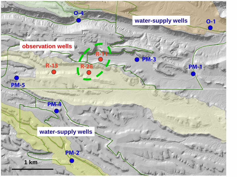
1 km

water-supply wells

water-supply wells

observation wells

0

2500

5000

0250050007500

10000

0250050007500

10000

0250050007500

10000

0250050007500

0100020003000

10/1/2004 4/1/2005 10/1/2005 4/1/2006 10/1/2006 4/1/2007 10/1/20070

250050007500

10000

PM-1

PM-2

PM-3

Daily

pro

duct

ion

volu

mes

, gal

lons

PM-4

PM-5

O-1

O-4

Pumping records (10/2004-12/2007)

~3-year record

Daily data

Unique patterns

PM-2, PM-5,and O-4 arethe major water producers(note the different scales of y-axes)

New data already available but have not been analyzed yet

5837

5838

5839

5849585058515852

5838

5839

5840

Raw data Baro corrected

R-11

Elev

atio

n, ft R-15

R-28

Water-level records (span ~3 years)~15 min-1h temporal resolution~3 ft (1 m) fluctuations at R-15~1 ft (0.3 m) fluctuations at R-11 and R-28;fluctuations at R-11 and R-28 are similar

Potential transient influences:• pumping effects• barometric effects • variability in the ambient flux• variability in local recharge• subsidence (pore-elastic effects)

2005 2006 2007 2008

5837

5838

5839

5849585058515852

5838

5839

5840

Raw data Baro corrected

R-11

Elev

atio

n, ft R-15

R-28

Water-level vs. pumping recordsVisual comparisons demonstrate correlations between the water levels and the pumping regimes. Goals:1. Fingerprint the pumping wells causing

the observed water-level fluctuations2. Estimate effective aquifer properties

using a simple analytical method3. Estimate aquifer heterogeneity using a

tomographic approach based on a simple numerical model 0

2500

5000

0250050007500

10000

0250050007500

10000

0250050007500

10000

0250050007500

0100020003000

10/1/2004 4/1/2005 10/1/2005 4/1/2006 10/1/2006 4/1/2007 10/1/20070

250050007500

10000

PM-1

PM-2

PM-3

Daily

pro

duct

ion

volu

mes

, gal

lons

PM-4

PM-5

O-1

O-4

Methodology of Approach 1: Analytical analysis Simple analytical model (Theis + superposition) taking into account the

pumping records of all the pumping wells (7) Pressure variations of each monitoring well (R-11, R-15, R-28) are

analyzed independently Calibration of the analytical model to reproduce observed pressures

variations using Levenberg-Marquardt algorithm As a result, effective large-scale properties (T & S) of the aquifer

between pumping and monitoring wells are estimated The same results could have been obtained if specially designated

pumping tests were conducted at each water-supply wells The numerical models are created and the obtained results are

analyzed using automated (interactive) pre- and post-processing. In this way, the models can easily be updated when new data become available Model-input files are automatically generated All the information (water levels, pumping records, well locations,

etc) is automatically extracted from a database and applied in the inverse models

==

TtSrW

TQuW

TQs

44)(

4

2

ππ

( )∑∑= =

−

−−

=N

i

M

j Qiji

ii

i

ijiji

ttTSrW

TQQ

s1 1

21

44π

s - drawdown (L), Q - pumping rate (L3T-1), T - transmissivity (L2T-1), W(u) - well function r - distance between the pumping well and observation well (L), S – storativity, t - time since pumping commenced (T).

N - number of pumping wells, Mi - number of pumping periods (i.e. number of pumping rate changes), Qij -pumping rate of well i during pumping period j, and tQij - time when the pumping rate changed at well i during pumping period j

Theis equation

Theis equation applying the principle of superposition

12/21/2004 12/21/2005 12/21/2006 12/21/2007

1779.2

1779.3

1779.4

1779.5

1779.6

Elev

atio

n, m

Predicted Observed

9/21/2004 9/21/2005 9/21/2006 9/21/20071782.6

1782.8

1783.0

1783.2

1783.4

1783.6

1783.8

Elev

atio

n, m

Predicted Observed

9/21/2004 9/21/2005 9/21/2006 9/21/20071779.4

1779.5

1779.6

1779.7

1779.8

1779.9

1780.0

Elev

atio

n, m

Predicted Observed

R-11

R-15

R-28

Inverse results using analytical method

>1,000 calibration targets

15 adjustable aquifer parameters in each inverse model: 7 effective T’s; 7 effective S’s; initial water level

The model fingerprints the pumping wells that produce the observed drawdown responses

Pumping wells that do not produce drawdown responses are rejected in the model by estimating effective properties that preclude pumping drawdowns (e.g. high T; low S)

Deconstruction of R-15 transients

Which pumping wells influence the water-level transients?

05000

10000 PM-2

0.00.20.40.6

05000

10000

Prod

uctio

n, g

al/d

ay PM-3

0.00.20.40.6

05000

10000

PM-5

PM-4

0.00.20.40.6

Drawdown, m

10/1/2004 10/1/2005 10/1/2006 10/1/20070

500010000

0.00.20.40.6

9/21/2004 9/21/2005 9/21/2006 9/21/20071782.6

1782.8

1783.0

1783.2

1783.4

1783.6

1783.8

Elev

atio

n, m

Predicted Observed

05000

10000PM-2

0.00.10.2

05000

10000

Prod

uctio

n, g

al/d

ay PM-3

0.00.10.2

05000

10000 PM-4

0.00.10.2

Drawdown, m

10/1/2004 10/1/2005 10/1/2006 10/1/20070

500010000

Temporal trend

0.00.10.2

12/21/2004 12/21/2005 12/21/2006 12/21/2007

1779.2

1779.3

1779.4

1779.5

1779.6

Elev

atio

n, m

Predicted Observed



05000

10000 PM-2

0.00.10.2

05000

10000PM-3

0.00.10.2 Drawdown, m

05000

10000

Prod

uctio

n, g

al/d

ay

PM-4

0.00.10.2

10/1/2004 10/1/2005 10/1/2006 10/1/20070

500010000

0.00.10.2

Temporal Trend

9/21/2004 9/21/2005 9/21/2006 9/21/20071779.4

1779.5

1779.6

1779.7

1779.8

1779.9

1780.0

Elev

atio

n, m

Predicted Observed



1 km

Information about aquifer heterogeneity deduced from analytical analyses

no response to O-4 pumping

no response to PM-1 and O-4 pumping

pronounced response to PM-2 pumping

R-11/28 did not respond to PM-5 pumping

R-11/28 have similar transients

Tomo-graphic analysis

PM-1 PM-2 PM-3 PM-4 PM-5 O-1 O-4R-11 - -1.5 -0.1 -1.1 - - -R-15 - -1.9 -1.5 -1.7 -1.5 - -R-28 - -1.5 -0.4 -1.2 - - -

Mean -1.2 -1.7Variance 0.4 2.8


PM-1 PM-2 PM-3 PM-4 PM-5 O-1 O-4R-11 - 3.5 4.0 3.2 - - -R-15 - 3.3 3.4 3.2 3.7 - -R-28 - 3.5 3.8 3.7 - - -

Mean 3.5 2.0Variance 0.069 2.1

log10 T [m2/d]

log10 S [-]

Inverse results using analytical methodEffective parameter estimates; if standard cross-hole pumping tests have been conducted at each water-supply well, similar parameter estimates would have been obtained

Methodology of Approach 2: Hydraulic Tomography Simple numerical model (2D, transient) taking into account the

pumping records of all the pumping wells Calibration of the numerical model to reproduce observed pressures

variations using Levenberg-Marquardt algorithm Pressure records of all the monitoring well (currently, R-11, R-15, R-28)

are simultaneously analyzed Spatial heterogeneity of the aquifer is estimated using a geostatistical

method (kriging and pilot points [de Marsily, 1976]) The numerical models are created and the obtained results are

analyzed using automated (interactive) pre- and post-processing. In this way, the models can easily be updated when new data become available Computational grids and input files are automatically generated All the information (water levels, pumping records, well locations,

etc) is automatically extracted from a database and applied in the inverse models

1779.2

1779.25

1779.3

1779.35

1779.4

1779.45

1779.5

1779.55

1779.6

1779.65

0 200 400 600 800 1000 1200

Wat

er-le

vel e

leva

tion

[m]

Well r11 Case pms-rs-gstat-v14.res

ObservedSimulated

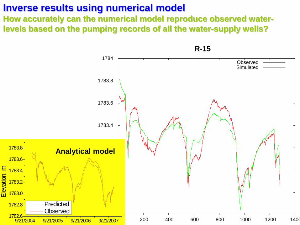
Inverse results using numerical modelHow accurately can the numerical model reproduce observed water-levels based on the pumping records of all the water-supply wells?

R-11

12/21/2004 12/21/2005 12/21/2006 12/21/2007

1779.2

1779.3

1779.4

1779.5

1779.6

Elev

atio

n, m

Predicted Observed

Analytical model

1782.6

1782.8

1783

1783.2

1783.4

1783.6

1783.8

1784

0 200 400 600 800 1000 1200 1400

Wat

er-le

vel e

leva

tion

[m]


ObservedSimulated

R-15

9/21/2004 9/21/2005 9/21/2006 9/21/20071782.6

1782.8

1783.0

1783.2

1783.4

1783.6

1783.8

Elev

atio

n, m

Predicted Observed

Analytical model


1779.4

1779.5

1779.6

1779.7

1779.8

1779.9

1780

0 200 400 600 800 1000 1200

Wat

er-le

vel e

leva

tion

[m]


ObservedSimulated

R-28


9/21/2004 9/21/2005 9/21/2006 9/21/20071779.4

1779.5

1779.6

1779.7

1779.8

1779.9

1780.0

Elev

atio

n, m

Predicted Observed

Analytical model

log10 T [m2/d]O-4

PM-1

PM-2

PM-3

PM-4

PM-5

R-11

R-15 R-28

-6

-5

-4

-3

-2

-1

0

1

O-4

PM-1

PM-2

PM-3

PM-4

PM-5

R-11

R-15 R-28

-1

0

1

2

3

4

5

6

7

0 m 500 m 1000 m 1500 m 2000 m

log10 S [-]

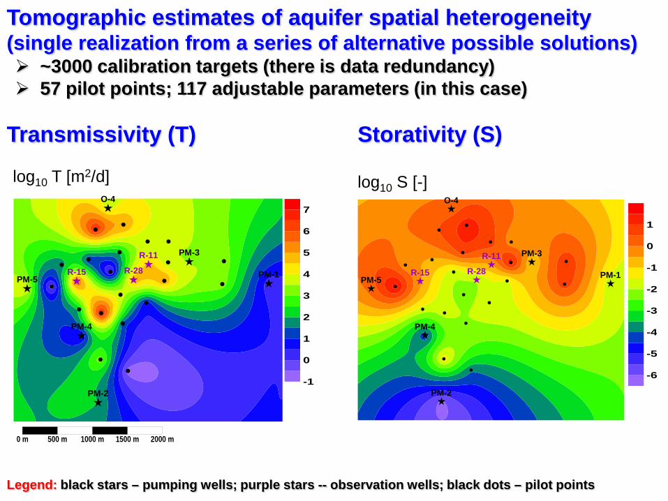
Tomographic estimates of aquifer spatial heterogeneity(single realization from a series of alternative possible solutions) ~3000 calibration targets (there is data redundancy) 57 pilot points; 117 adjustable parameters (in this case)

Storativity (S)Transmissivity (T)

Legend: black stars – pumping wells; purple stars -- observation wells; black dots – pilot points

log10 T [m2/d]O-4

PM-1

PM-2

PM-3

PM-4

PM-5

R-11

R-15 R-28

-1

0

1

2

3

4

5

6

7

0 m 500 m 1000 m 1500 m 2000 m

Estimated aquifer spatial heterogeneity

Aquifer structure deduced from the analytical analyses

Tomographic estimate of transmissivity (T)

1 km

Uniform (analytical) analysis


PM-1 PM-2 PM-3 PM-4 PM-5 O-1 O-4R-11 - -1.5 -0.1 -1.1 - - -R-15 - -1.9 -1.5 -1.7 -1.5 - -R-28 - -1.5 -0.4 -1.2 - - -

Mean -1.2 -1.7Variance 0.4 2.8

Uniform (analytical) analysis


PM-1 PM-2 PM-3 PM-4 PM-5 O-1 O-4R-11 - 3.5 4.0 3.2 - - -R-15 - 3.3 3.4 3.2 3.7 - -R-28 - 3.5 3.8 3.7 - - -

Mean 3.5 3.0Variance 0.069 2.1

log10 T [m2/d]

log10 S [-]

Compared to the non-uniform analyses, uniform analyses overestimate the mean aquifer properties, and underestimate the aquifer heterogeneity (variances)

Uniform case: variability in T suggests pronounced aquifer heterogeneity (non-stationarity) Uniform case: var(S) > var(T). Non-uniform case: var(T) ≈ var(S); var(S) is still substantial

(this may be real or caused by 3D or other effects unaccounted in the conceptual model)

ConclusionsResults are consistent with previous work related to scaling effects of aquifer properties [e.g. Gelhar, 1993, Dagan and Neuman, 1997; Meier at al., 1998; Sanchez-Villa, 1999; Vesselinov at al., 2001, etc.]

Conclusions (cont.) Tomographic analysis based on long-term (3 year) production and

water-level records is successfully applied to extract information about the large-scale properties of the regional aquifer

Pumping influences of individual pumping wells are fingerprinted despite the small magnitudes of observed drawdowns

Analysis of the results based on a simple analytical model suggests that there may be large-scale hydrogeologic structures (faults and troughs) with contrasting aquifer properties

Similar estimates of aquifer heterogeneity are also obtained using the tomographic analysis based on numerical model

Information content of the data collected during previous pumping tests (at PM-2, PM-4) is much inferior to the information content of the data collected during long-term water-supply pumping

This is a novel and unique research work; similar analyses have not been previously published in the hydrogeologic literature

Potential future work: Include longer water-level/pumping records and more monitoring wells Evaluate uncertainty in estimates of aquifer heterogeneity Extend the analysis to 3D tomography

Estimation of aquifer properties based on pressure ...

Documents

Transcript of Estimation of aquifer properties based on pressure ...