Estimation of an Equilibrium Model with Externalities ...cfu/Fu_Gregory.pdf · Estimation of an...

Estimation of an Equilibrium Model with Externalities:

Post-Disaster Neighborhood Rebuilding∗

Chao Fu and Jesse Gregory

University of Wisconsin and NBER

Abstract

We study the optimal design of subsidies in an equilibrium setting, where the deci-

sions of individual recipients impose externalities on one another. We apply the model

to the case of post-Katrina rebuilding in New Orleans under the Louisiana Road Home

rebuilding grant program (RH). We estimate the structural model via indirect infer-

ence, exploiting a discontinuity in the formula for determining the size of grants, which

helps isolate the causal effect of neighbors’ rebuilding on one’s own rebuilding choices.

We find that the additional rebuilding induced by RH generated positive externalities

equivalent to $4,950 to each inframarginal household whose rebuilding choice was not

affected by the program. Counterfactual policy experiments find that optimal sub-

sidy policies bias grant offers against relocation, with an inverse-U-shaped relationship

between the degree of bias and the severity of damages from the disaster.

∗We thank Zach Flynn and Chenyan Lu for excellent research assistance. We thank Steven Durlauf, JohnKennan, Chris Taber, and Jim Walker for insightful discussions. We thank the editor and two anonymousreferees for their suggestions. We have also benefited from helpful comments and suggestions by seminarparticipants at Berkeley, the Cleveland Fed, Depaul, Duke, Iowa, Michigan, Penn, Rochester, Stanford-GSB,UCLA, UIC, UW-Milwaukee, and Wash U. All errors are ours.

1 Introduction

Individuals’ choices are sometimes inevitably and endogenously inter-related due to spillover

effects from one’s choices onto others’ payoffs. These spillovers are often not accounted for

when individuals make their decisions, which may lead to inefficient equilibrium outcomes

and hence leave space for policy interventions.1 Effective policy designs require the capability

of predicting and comparing the impacts of alternative counterfactual policies, which in turn

relies on two essential pieces of information: 1) the nature of the spillover effects, which can

be difficult to identify,2 and 2) how decisions are made in equilibrium and how equilibrium

outcomes differ across counterfactual policy environments. In this paper, we develop a unified

framework to obtain both pieces of information.

To place our framework in a concrete setting, we study the rebuilding of neighborhoods

affected by Hurricane Katrina under the Louisiana Road Home program (RH). RH offered

rebuilding grant packages and less generous relocation grant packages to all Katrina-affected

homeowners in the state with uninsured losses. The RH grant formula yielded significantly

larger grant offers when an index measuring home damages fell above a particular threshold.

As a result, otherwise similar households with index values just above/below this threshold

faced very different financial incentives to rebuild. Using a regression discontinuity design

(RDD) on the administrative micro-level data, we find robust evidence of non-linear spillover

effects among neighbors’ rebuilding decisions. Households just above the threshold where

the incentive to rebuild jumps discontinuously were 5.0 percentage points more likely to

rebuild than otherwise similar households just below that threshold. Neighbors of these

households, whose financial incentives were not directly affected, were 2.4 percentage points

more likely to rebuild, suggesting the existence of sizable spillover effects. Moreover, the size

of spillovers varied significantly across neighborhoods, suggesting that spillover effects are

likely to be non-linear.

To achieve the goal of studying the effectiveness of alternative (counterfactual) policy

designs, one needs to go beyond RDD analyses and to understand the fundamental factors

driving equilibrium outcomes. We develop an equilibrium model of neighbors’ post-disaster

rebuilding choices with amenity spillovers. Households have private preferences for consump-

tion and for residing in their home. They also derive utility from a neighborhood amenity

1For instance, negative spillovers from home foreclosures are a commonly cited motivation for subsidizedmortgage modifications (Cambell, Giglio, Pathak, 2010). Arguments against rent controls often cite thepossibility that undermaintained properties reduce the value of nearby non-controlled properties (Autor,Palmer, and Pathak, 2012).

2Manski (1993) raises the reflection problem. Brock and Durlauf (2007) show that point identification ofsocial interactions can fail even when there is no reflection problem in settings where important group-levelvariables are not observed by the researcher.

1

that depends on the fraction of neighbors who rebuild, an externality that is not internal-

ized by individual households. In each period, households who have not yet rebuilt or sold

their houses have the option to rebuild, sell or wait. Households’ decisions are inter-related

because of amenity spillovers. An equilibrium requires that individuals’ decisions be best

responses to each other. Given the RDD evidence of non-linear spillover effects, we embed

in our structural model a flexible amenity spillover function. The identification of our model

with such a flexible spillover function is achieved via indirect inference that fully exploits the

discontinuity in the RH grant formula.

The estimated model reveals important policy implications arising from amenity spillovers.

RH’s full equilibrium impact on the city-wide rebuilding rate, including “feedback” effects

from positive amenity spillovers, was 27% larger than the impact generated by the pro-

gram’s financial incentives alone (holding amenities fixed). Like many other disaster relief

packages, RH provided a higher financial incentive to rebuild than to relocate. Although

the conditional nature of the program created excess burden by distorting privately opti-

mal resettlement choices, the spillover effects were strong enough such that the net average

household welfare was $2,177 higher under RH than it would have been had households been

offered the same grant regardless of whether they chose to rebuild or to relocate.

Our framework is well-suited for exploring a wide range of policy interventions with

various goals and/or constraints. For illustration, we examine the possibility of further

improving welfare by studying a particular group of conditional grant policies, which offer a

fraction (1−ρ) of the RH rebuilding grant to households if they choose to relocate. We search

for the optimal ρ’s given different constraints. Compared to the case under the unconditional

grant policy, net average household welfare would improve by $2,638 if ρ’s are restricted to

be the same for all households, by $3,613 if ρ’s can differ by flooding severity, and by over

$6,000 if ρ’s can be block-specific. The relationship is inversed-U-shaped between the optimal

penalties against relocation (ρ) and the severity of damages from the disaster, with greater

biases against relocation for areas with moderate damages.

Although our empirical application focuses on a special event, our equilibrium modeling

framework can be applied/extended to other cases where individual decisions inter-relate due

to spillover effects. Our findings highlight the fact that, when externalities potentially exist,

accounting for equilibrium interactions among individuals and quantifying the externality

is essential for the design of policies. To shed light on policy designs with relatively less

restrictive modeling assumptions for identification, our paper combines the strengths of two

strands of the literature on spillover effects, one relying on quasi-experiments and the other

on structural models.

Consistent with our estimates, reduced-form analyses in the first strand of literature

2

have found evidence that policies stimulating investment in housing boost the value of nearby

homes not directly affected by the policies (Autor, Palmer, and Pathak 2012; Rossi-Hansberg,

Sarte, and Owens 2010), and that negative spillover effects of foreclosures are larger for more

proximate homes (Campbell, Giglio, and Pathak 2011; Harding, Rosenblatt, and Yao 2009).

In the second strand of literature, de Paula (2009) is the closest to our work.3 He studies

inference in a continuous time model where an agent’s payoff to quit an activity depends on

the participation of other players. Ours is a discrete time model where neighbors’ choices

of the timing of rebuilding are inter-related. Our paper embeds variation from a quasi-

experiment in our structural model to estimate the shape and strength of social spillovers.4

Although experimentally-generated variation in incentives is not always available, differ-

ent and more general identification strategies than the one used in this paper are available,

which typically require more structure on, for example, the selection into groups/neighborhoods.5

For example, Brock and Durlauf (2006) and Brock and Durlauf (2007) provide methods for

identifying social interactions in discrete choice models with endogenous group formation.

Brock and Durlauf (2007) demonstrate partial identification of social interactions with un-

observed neighborhood-level covariates. Bayer and Timmins (2007) propose an instrument

for peers’ behavior that is based on exogenous location characteristics and motivated by a

formal location choice model to identify spillovers.

Our paper is also related to the literature studying the post-Hurricane-Katrina locations,

labor market outcomes, and wellbeing of displaced New Orleans residents.6 Most closely

related to our paper, Gregory (2014) estimates a structural individual decision model of

New Orleans homeowners’ resettlement choices. Gregory (2014) uses the estimated model

to study the trade-off of post-disaster bailouts between their short run insurance benefits

and the long run efficiency losses caused by expected future bailouts distorting households’

location choices (moral hazards). Instead of treating each household in isolation, our paper

emphasizes the possible spillover effects from individual households’ choices and the inter-

related nature of households’ choices in an equilibrium context. We study the optimal design

of conditional subsidies that internalize spillover effects and improve household welfare in

3Other recent examples of equilibrium model-based approaches to studying housing and/or locationchoices include; Epple and Sieg (1999); Epple, Romer, and Sieg (2001); Ioannides (2003); Bayer, McMillan,and Reuben (2005); Bayer, Ferreira, and McMillan (2007); Bayer and Timmins (2007); and Ioannides andZabel (2008).

4Galiani, Murphy, and Pantano (2012) use the experimentally randomized variation in neighborhood-specific financial incentives from the Moving to Opportunity (MTO) demonstration to identify the structuralparameters of an individual neighborhood choice model (without social interactions).

5See Blume, Brock, Durlauf, and Ioannides (2010) for a comprehensive review of the literature on theidentification of social interaction effects.

6For example, Groen and Polivka, 2010; Zissimopolous and Karoly, 2010; Vigdor, 2007 and 2008; Paxsonand Rouse, 2008; and Elliott and Pais, 2006.

3

equilibrium.

The rest of the paper is organized as follows: Section 2 provides additional policy back-

ground. Section 3 describes our dataset and RDD results. Section 4 describes the structural

equilibrium model. Section 5 explains our estimation. Section 6 presents the estimation

results. Section 7 presents our counterfactual experiments, and Section 8 concludes. Addi-

tional details are provided in the appendix.

2 Background Information

Hurricane Katrina struck the U.S. Gulf Coast on August 29, 2005. The storm and subsequent

flooding left two thirds of the city’s housing stock uninhabitable without extensive repairs,

the costs of which significantly exceeded insurance payouts for many pre-Katrina homeowners

in New Orleans. Among the nearly 460,000 displaced residents, many spent a considerable

amount of time away from the city or never returned. Congress approved supplemental relief

block grants to the Katrina-affected states. Possible uses of these grants were hotly debated,

with proposals ranging from mandated buyouts to universally subsidized reconstruction.

The state of the Louisiana used its federal allocation to create the Louisiana Road Home

program, which provided cash grants for rebuilding or relocating to pre-Katrina Louisiana

homeowners with uninsured damages.7

A participating household could accept its RH grant as a rebuilding grant or as a reloca-

tion grant. Subject to an upper limit of $150,000, both grant types provided compensation

equal to the “value of home damages” minus the value of any insurance payouts already

received. The RH grant formula yielded significantly larger grant offers when an index

measuring home damages fell above a particular threshold. There were several important

differences between rebuilding and relocation grants. While both provided the same cash

payout,8 relocation grant recipients were required to turn their properties over to a state

7Other policies targeted to the Gulf Coast in the aftermath of Hurricane Katrina included Federal Emer-gency Management Agency (FEMA) small assistance grants in the hurricane’s immediate aftermath andGulf Opportunity Zone subsidies to firms for capital reinvestments and the hiring and retention of displacedworkers. The program other than RH that most directly impacted homeowners’ ability to rebuild was theSmall Business Administration (SBA) Disaster Loan program, which provided loans to homeowners withuninsured damages who met certain credit standards. The SBA Disaster Loan program is a standing pro-gram that, despite being federally subsidized, has non-trivial credit standards, and the program rejected alarge majority of applicants from the Gulf Coast in the aftermath of Katrina (Eaton and Nixon, 2005). Forthat reason, we allow for the possibility of credit constraints in our equilibrium model.

8The cash grants for relocating and for rebuilding were the same except for one particular circumstance.All RH grants were initially capped at the pre-Katrina value of a household’s home. For households clas-sified as “low or moderate income,” this cap was waved for rebuilding grants (in response to the argumentthat the provision had disparate impacts by race, because identical homes had different market values inpredominantly black versus white neighborhoods) but not for relocation grants.

4

land trust. For households with partial home damages, this stipulation introduced a sizable

opportunity cost to relocating. On the other hand, rebuilding grant recipients were only

required to sign covenant agreements to use their grants for rebuilding and to not sell their

homes for at least three years. We provide additional details in Section 4.2 on the incentive

effects of these program rules and differences in these incentives on either side of the grant

formula discontinuity.

Grant recipients often experienced lengthy delays between initiating their grant applica-

tions and receiving a grant. RH was announced in February, 2006, but the median grant

payment date occurred after Katrina’s second anniversary in 2007, which is captured in our

model. Despite the program’s slow rollout, RH had disbursed nearly ten billion dollars to

Louisiana homeowners by Katrina’s fifth anniversary.

3 Data, Policy Details, and RDD Analyses

3.1 Data

The main data for our analysis are the administrative property records of the Orleans Parish

Assessor’s Office (Assessor’s property data) and the administrative program records of the

Louisiana Road Home grant program (RH data). The Assessor’s property data provide

information on the timing of home repairs and home sales for the full universe of New

Orleans properties. For each property, the data provide annual appraised land and structure

values for 2004-2010, which we use to infer the timing of home repairs, and the date and

transaction price of all post-Katrina home sales.

The RH data provide detailed information on the grant amount offered to each applicant

household and whether the applicant chose a rebuilding grant (which required the household

to rebuild and not to sell for at least three years), a relocation grant (which required the

household to turn its property over to a state land trust with no additional compensation

for any as-is value of the property), or chose not to participate. The data also include all of

the inputs to the RH grant offer formula; including a repair cost appraisal and a replacement

cost appraisal for each home, and the total value of private insurance payments paid to each

household. Together with the RH grant formula, such information enables us to compute

both types of RH grants for each household regardless of its actual choice.

We merge the RH data and the Assessor’s property data at the property level by street

address. We also obtain measures of the depth of flooding on each Census block from a

FEMA-provided data set created from satellite images, and the demographic composition

of each Census block from the 2000 Census. Because our focus is on spillover effects from

5

homeowners’ rebuilding choices, we exclude homes that were renter-occupied when Katrina

occurred and Census blocks that contained fewer than five owner-occupied homes. The

resulting dataset contains 60,175 households living in 4,795 blocks.

Solving our model requires a measure of the wages available to each household in and

away from New Orleans {w1it, w

0it}t. We impute these variables with a two step procedure

that combines data from the Displaced New Orleans Residents Survey (DNORS)9 on the

distribution of earnings and occupations in New Orleans during the year prior to Katrina

and data from the American Community Survey (ACS) on occupation-specific trends in

prevailing wages across labor markets from 2005-2010. The first step uses nearest Maha-

lanobis distance matching to assign each household a “donor” DNORS record. The second

step imputes Post-Katrina wage offers by adjusting the household head’s and spouse’s pre-

Katrina annual earnings by an occupation-MSA-specific wage index estimated with ACS

data (see details in online Appendix II). The imputed wage measures capture the fact that

the incentive to return to New Orleans varied across households of different occupations

(e.g. construction wages increased and personal service wages fell post-Katrina). Because

of the extent of imputation in these variables, we do not exploit variation in labor market

incentives for identification.

Lastly, we use data from the Federal Reserve Bank of New York Consumer Credit

Panel/Equifax to obtain information on neighborhood-level credit conditions. These data

cannot be merged at the household level to our other data sources. Instead, we compute the

average Equifax Risk Score (TM) within 1/4 mile of each block’s centroid, and assign each

household a simulated credit score riski ∼ N(riskbuf(i), 85), where riskbuf(i) is the average

risk-score calculated for household i’s block and 85 is the within-block standard deviation of

risk scores.10

3.1.1 Summary Statistics

Table 1 presents descriptive statistics for our sample of homeowning households (Column 1)

and the subsample of households whose houses were damaged and left unlivable by Katrina

(Column 2). Forty-six percent of households lived in areas that received less than 2 feet of

flooding, while over 20% of households were from areas that received over 5 feet of flooding.

9Fielded by RAND in 2009 and 2010, the Displaced New Orleans Residents Survey located and intervieweda population-representative 1% sample of the population who had been living in New Orleans just prior toHurricane Katrina.

10It would be ideal to allow credit scores to vary systematically by household characteristics within ablock. Our cruder approach to modeling credit availability is driven by a data limitation, namely that weobserve a “spatial moving average” of credit scores but not microdata. Given the high degree of both racialand economic segregation in New Orleans, however, we do not expect that conditioning credit score drawson additional observables within neighborhoods would change our results in a meaningful way.

6

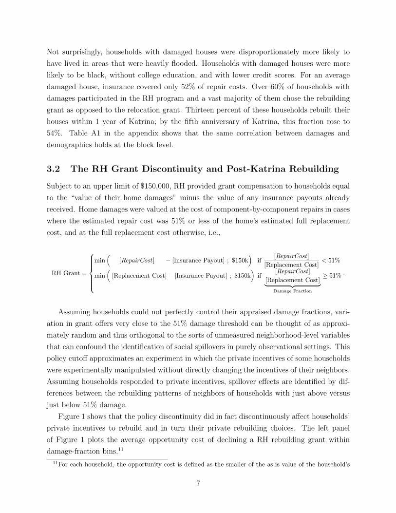
Not surprisingly, households with damaged houses were disproportionately more likely to

have lived in areas that were heavily flooded. Households with damaged houses were more

likely to be black, without college education, and with lower credit scores. For an average

damaged house, insurance covered only 52% of repair costs. Over 60% of households with

damages participated in the RH program and a vast majority of them chose the rebuilding

grant as opposed to the relocation grant. Thirteen percent of these households rebuilt their

houses within 1 year of Katrina; by the fifth anniversary of Katrina, this fraction rose to

54%. Table A1 in the appendix shows that the same correlation between damages and

demographics holds at the block level.

3.2 The RH Grant Discontinuity and Post-Katrina Rebuilding

Subject to an upper limit of $150,000, RH provided grant compensation to households equal

to the “value of their home damages” minus the value of any insurance payouts already

received. Home damages were valued at the cost of component-by-component repairs in cases

where the estimated repair cost was 51% or less of the home’s estimated full replacement

cost, and at the full replacement cost otherwise, i.e.,

RH Grant =

min

([RepairCost ] − [Insurance Payout] ; $150k

)if

[RepairCost ]

[Replacement Cost]< 51%

min(

[Replacement Cost]− [Insurance Payout] ; $150k)

if[RepairCost ]

[Replacement Cost]︸︷︷︸Damage Fraction

≥ 51% .

Assuming households could not perfectly control their appraised damage fractions, vari-

ation in grant offers very close to the 51% damage threshold can be thought of as approxi-

mately random and thus orthogonal to the sorts of unmeasured neighborhood-level variables

that can confound the identification of social spillovers in purely observational settings. This

policy cutoff approximates an experiment in which the private incentives of some households

were experimentally manipulated without directly changing the incentives of their neighbors.

Assuming households responded to private incentives, spillover effects are identified by dif-

ferences between the rebuilding patterns of neighbors of households with just above versus

just below 51% damage.

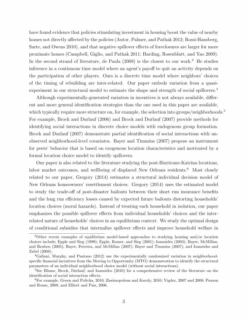
Figure 1 shows that the policy discontinuity did in fact discontinuously affect households’

private incentives to rebuild and in turn their private rebuilding choices. The left panel

of Figure 1 plots the average opportunity cost of declining a RH rebuilding grant within

damage-fraction bins.11

11For each household, the opportunity cost is defined as the smaller of the as-is value of the household’s

7

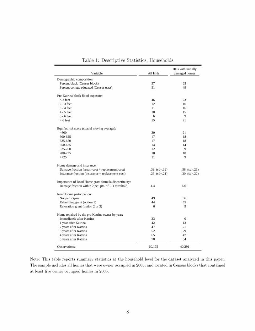
Table 1: Descriptive Statistics, Households

Variable All HHs

HHs with initially

damaged homes

Demographic composition:

Percent black (Census block) 57 65

Percent college educated (Census tract) 51 49

Pre-Katrina block flood exposure:

< 2 feet 46 23

2 - 3 feet 12 16

3 - 4 feet 11 16

4 - 5 feet 10 15

5 - 6 feet 6 9

> 6 feet 15 21

Equifax risk score (spatial moving average):

<600 20 21

600-625 17 18

625-650 17 18

650-675 14 14

675-700 12 9

700-725 10 10

>725 11 9

Home damage and insurance:

Damage fraction (repair cost ÷ replacement cost) .39 (sd=.32) .58 (sd=.21)

Insurance fraction (insurance ÷ replacement cost) .23 (sd=.21) .30 (sd=.22)

Importance of Road Home grant formula discontinuity:

Damage fraction within 2 pct. pts. of RD threshold 4.4 6.6

Road Home participation:

Nonparticipant 49 36

Rebuilding grant (option 1) 44 55

Relocation grant (option 2 or 3) 6 9

Home repaired by the pre-Katrina owner by year:

Immediately after Katrina 33 0

1 year after Katrina 42 13

2 years after Katrina 47 21




Observations: 60,175 40,291

Note: This table reports summary statistics at the household level for the dataset analyzed in this paper.

The sample includes all homes that were owner occupied in 2005, and located in Census blocks that contained

at least five owner occupied homes in 2005.

8

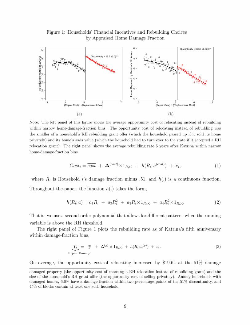
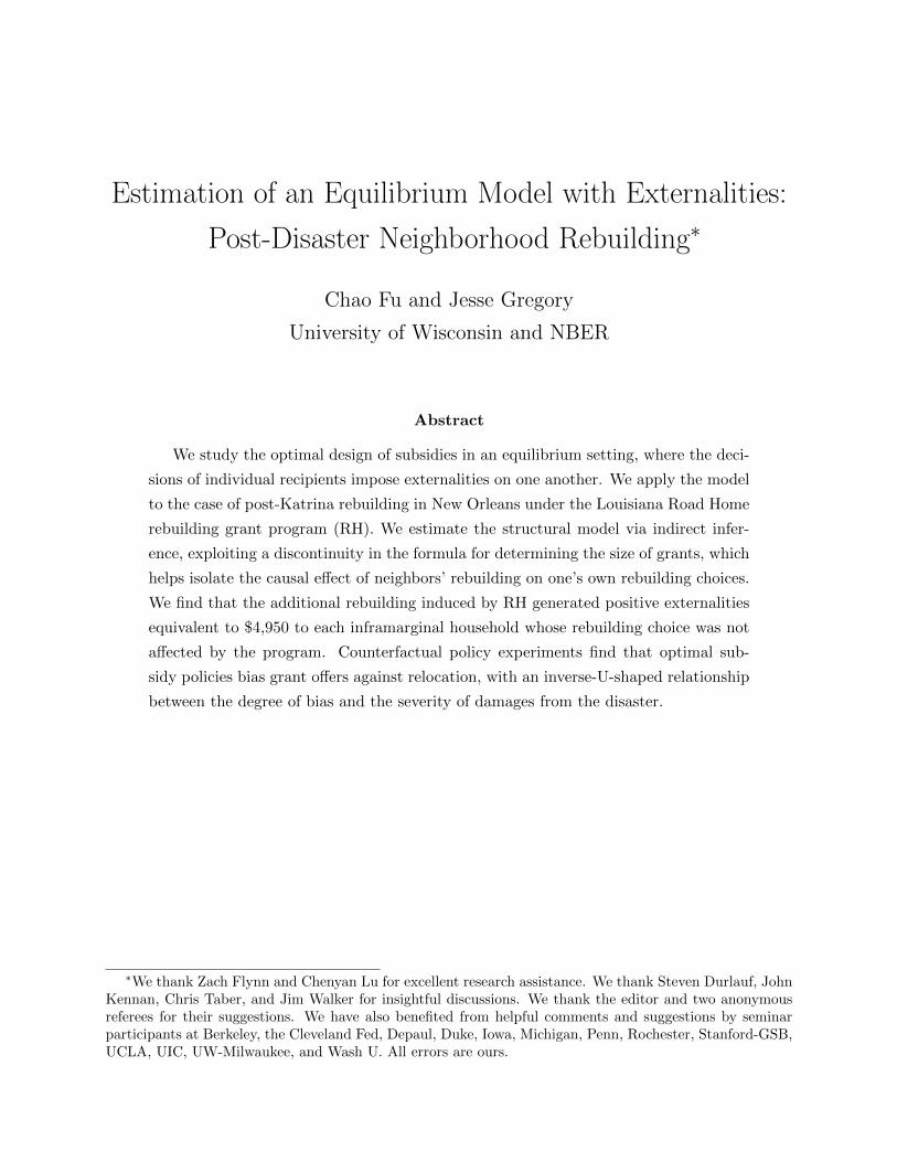
Figure 1: Households’ Financial Incentives and Rebuilding Choicesby Appraised Home Damage Fraction

Discontinuity = 19.6 (1.0)***

010

2030

4050

60In

cent

ive

to R

ebui

ld (

$100

0s)

.3 .4 .5 .6 .7(Repair Cost) ÷ (Replacement Cost)

(a)

Discontinuity = 0.050 (0.020)**

.3.4

.5.6

.7.8

Hom

e R

epai

red

by K

atrin

a’s

5th

Ann

iv.


(b)

Note: The left panel of this figure shows the average opportunity cost of relocating instead of rebuilding

within narrow home-damage-fraction bins. The opportunity cost of relocating instead of rebuilding was

the smaller of a household’s RH rebuilding grant offer (which the household passed up if it sold its home

privately) and its home’s as-is value (which the household had to turn over to the state if it accepted a RH

relocation grant). The right panel shows the average rebuilding rate 5 years after Katrina within narrow

home-damage-fraction bins.

Costi = cost + ∆(cost)×1Ri>0 + h(Ri; a(cost)) + ei, (1)

where Ri is Household i’s damage fraction minus .51, and h(.) is a continuous function.

Throughout the paper, the function h(.) takes the form,

h(Ri; a) = a1Ri + a2R2i + a3Ri×1Ri>0 + a4R

2i×1Ri>0 (2)

That is, we use a second-order polynomial that allows for different patterns when the running

variable is above the RH threshold.The right panel of Figure 1 plots the rebuilding rate as of Katrina’s fifth anniversary

within damage-fraction bins,

Yi︸︷︷︸Repair Dummy

= y + ∆(y) × 1Ri>0 + h(Ri; a(y)) + ei. (3)

On average, the opportunity cost of relocating increased by $19.6k at the 51% damage

damaged property (the opportunity cost of choosing a RH relocation instead of rebuilding grant) and thesize of the household’s RH grant offer (the opportunity cost of selling privately). Among households withdamaged homes, 6.6% have a damage fraction within two percentage points of the 51% discontinuity, and45% of blocks contain at least one such household.

9

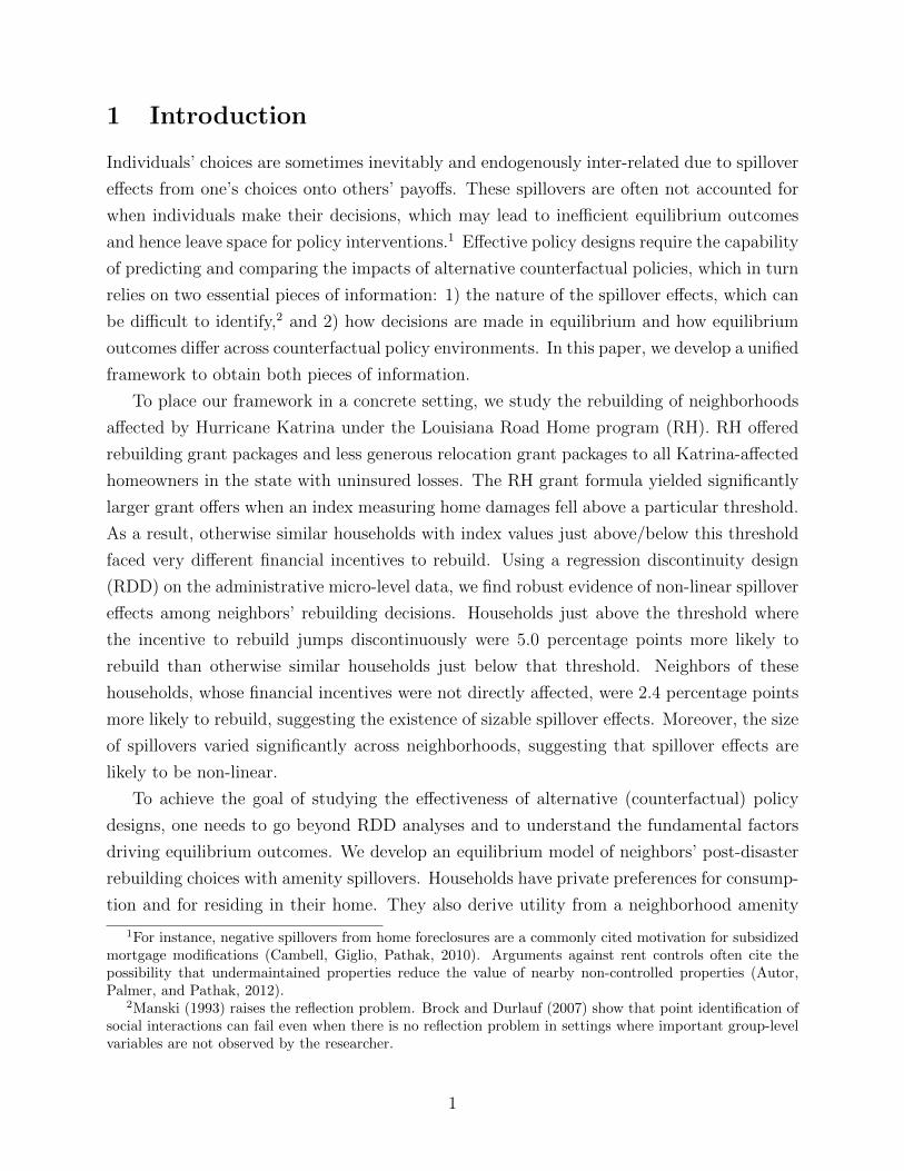
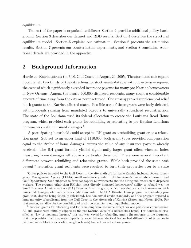
Figure 2: Distribution of Appraised Home Damage Fractions

H0: Discontinuity=0 (p=0.064*)

13

5D

ensi

ty

.4 .5 .6Post−appeal: (Repair Cost) ÷ (Replacement Cost)

(a)

H0: Discontinuity=0 (p=0.533)

13

5D

ensi

ty

.4 .5 .6(Repair Cost) ÷ (Replacement Cost)

(b)

01

23

45

Den

sity

0 .25 .5 .75 1(Repair Cost) ÷ (Replacement Cost)

(c)

Note: Panel (a) of this figure plots the density of RH-appraised home damage fractions (repair cost ÷replacement cost) close to the 51% RH grant threshold once all appeals of initial appraisals had been

adjudicated. Panel (b) plots the density of initial RH-appraised home damage fractions close to the 51%

grant-offer threshold. Panel (c) shows the full distribution of RH-appraised damage fractions.

threshold, and the probability of rebuilding increases by 5.0 percentage points.12

3.2.1 Validity Tests

This quasi-experiment is only credible if households were unable to perfectly control the value

of their “damage fraction” running variable relative to the 51% damage threshold. Panels

(a) and (b) of Figure 2 compute McCrary tests for continuity in the density of damage

fractions at 51% based on two different definitions of the damage fraction variable. The

damage fraction in panel (a) is based on households’ final damage appraisals, incorporating

the adjudicated decisions on all household appeals of initial damage appraisals, and exhibits a

somewhat larger density just above 51% than just below 51% (p=.064). The damage fraction

in panel (b) is based on households’ initial damage appraisals. A McCrary test applied

to these “first-appraisal” damage fractions fails to reject continuity at the 51% threshold

(p=0.533). We therefore treat the first-appraisal damage fraction as the running variable in

all substantive analyses. Panel (c) confirms that a non-trivial portion of the overall damage-

fraction distribution falls near the 51% threshold.

Table 2 assesses the balance of pre-determined covariates above and below the 51%

threshold. Columns (1) and (2) report each variable’s mean among households with just

below and just above 51% damage. Column (3) reports the p-value of the null that the

two are equal.13 These tests fail to reject the null of balance for any covariates; including

the fraction of same-block neighbors with undamaged homes, block-level demographics and

12Appendix Table A2 shows that these results are robust to alternative specifications, including local linearregression using an optimal bandwidth (Calononico, Catteneo, and Titiunik 2014).

13We restrict the sample to households with a damage fraction between 0.33 and 0.67, and for each variable

10

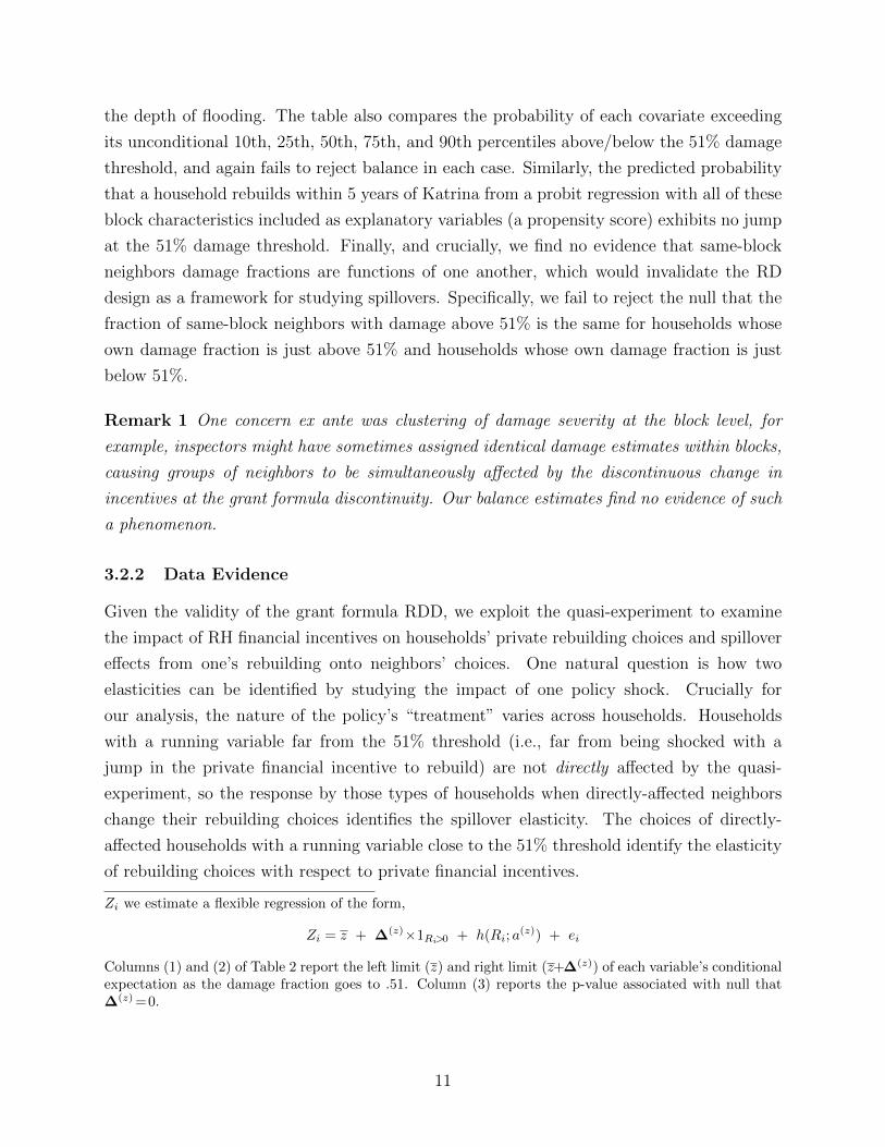
the depth of flooding. The table also compares the probability of each covariate exceeding

its unconditional 10th, 25th, 50th, 75th, and 90th percentiles above/below the 51% damage

threshold, and again fails to reject balance in each case. Similarly, the predicted probability

that a household rebuilds within 5 years of Katrina from a probit regression with all of these

block characteristics included as explanatory variables (a propensity score) exhibits no jump

at the 51% damage threshold. Finally, and crucially, we find no evidence that same-block

neighbors damage fractions are functions of one another, which would invalidate the RD

design as a framework for studying spillovers. Specifically, we fail to reject the null that the

fraction of same-block neighbors with damage above 51% is the same for households whose

own damage fraction is just above 51% and households whose own damage fraction is just

below 51%.

Remark 1 One concern ex ante was clustering of damage severity at the block level, for

example, inspectors might have sometimes assigned identical damage estimates within blocks,

causing groups of neighbors to be simultaneously affected by the discontinuous change in

incentives at the grant formula discontinuity. Our balance estimates find no evidence of such

a phenomenon.

3.2.2 Data Evidence

Given the validity of the grant formula RDD, we exploit the quasi-experiment to examine

the impact of RH financial incentives on households’ private rebuilding choices and spillover

effects from one’s rebuilding onto neighbors’ choices. One natural question is how two

elasticities can be identified by studying the impact of one policy shock. Crucially for

our analysis, the nature of the policy’s “treatment” varies across households. Households

with a running variable far from the 51% threshold (i.e., far from being shocked with a

jump in the private financial incentive to rebuild) are not directly affected by the quasi-

experiment, so the response by those types of households when directly-affected neighbors

change their rebuilding choices identifies the spillover elasticity. The choices of directly-

affected households with a running variable close to the 51% threshold identify the elasticity

of rebuilding choices with respect to private financial incentives.

Zi we estimate a flexible regression of the form,

Zi = z + ∆(z)×1Ri>0 + h(Ri; a(z)) + ei

Columns (1) and (2) of Table 2 report the left limit (z) and right limit (z+∆(z)) of each variable’s conditionalexpectation as the damage fraction goes to .51. Column (3) reports the p-value associated with null that∆(z) =0.

11

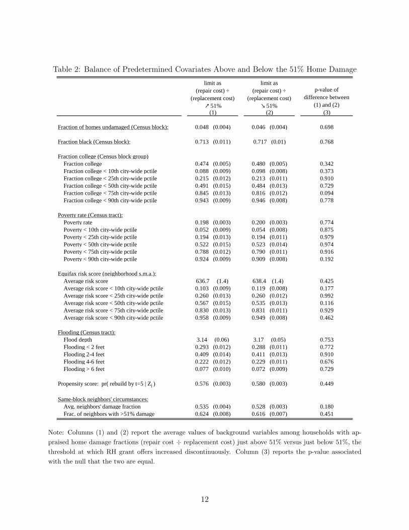
Table 2: Balance of Predetermined Covariates Above and Below the 51% Home Damage

limit as

(repair cost) ÷

(replacement cost)

↗ 51%

limit as

(repair cost) ÷

(replacement cost)

↘ 51%

p-value of

difference between

(1) and (2)

(1) (2) (3)

Fraction of homes undamaged (Census block): 0.048 (0.004) 0.046 (0.004) 0.698

Fraction black (Census block): 0.713 (0.011) 0.717 (0.01) 0.768

Fraction college (Census block group)

Fraction college 0.474 (0.005) 0.480 (0.005) 0.342

Fraction college < 10th city-wide pctile 0.088 (0.009) 0.098 (0.008) 0.373





Poverty rate (Census tract):

Poverty rate 0.198 (0.003) 0.200 (0.003) 0.774

Poverty < 10th city-wide pctile 0.052 (0.009) 0.054 (0.008) 0.875





Equifax risk score (neighborhood s.m.a.):

Average risk score 636.7 (1.4) 638.4 (1.4) 0.425

Average risk score < 10th city-wide pctile 0.103 (0.009) 0.119 (0.008) 0.177





Flooding (Census tract):

Flood depth 3.14 (0.06) 3.17 (0.05) 0.753

Flooding < 2 feet 0.293 (0.012) 0.288 (0.011) 0.772

Flooding 2-4 feet 0.409 (0.014) 0.411 (0.013) 0.910

Flooding 4-6 feet 0.222 (0.012) 0.229 (0.011) 0.676

Flooding > 6 feet 0.077 (0.010) 0.072 (0.009) 0.729

Propensity score: pr( rebuild by t=5 | Zj ) 0.576 (0.003) 0.580 (0.003) 0.449

Same-block neighbors' circumstances:

Avg. neighbors' damage fraction 0.535 (0.004) 0.528 (0.003) 0.180

Frac. of neighbors with >51% damage 0.624 (0.008) 0.616 (0.007) 0.451

Note: Columns (1) and (2) report the average values of background variables among households with ap-

praised home damage fractions (repair cost ÷ replacement cost) just above 51% versus just below 51%, the

threshold at which RH grant offers increased discontinuously. Column (3) reports the p-value associated

with the null that the two are equal.

12

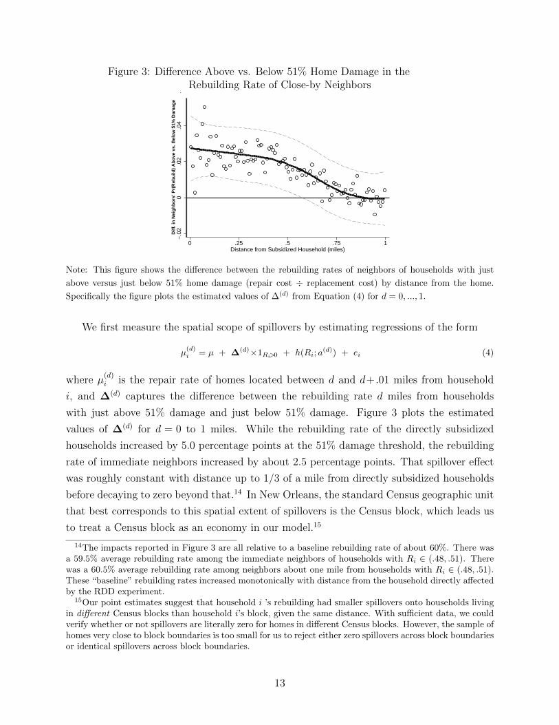
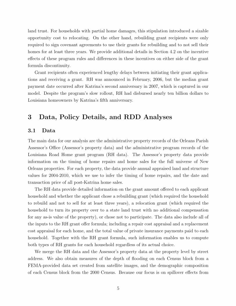
Figure 3: Difference Above vs. Below 51% Home Damage in theRebuilding Rate of Close-by Neighbors

−.0

20

.02

.04

.06

Dif

f. in

Nei

gh

bo

rs’ P

r(R

ebu

ild)

Ab

ove

vs.

Bel

ow

51%

Dam

age

0 .25 .5 .75 1Distance from Subsidized Household (miles)

Note: This figure shows the difference between the rebuilding rates of neighbors of households with just

above versus just below 51% home damage (repair cost ÷ replacement cost) by distance from the home.

Specifically the figure plots the estimated values of ∆(d) from Equation (4) for d = 0, ..., 1.

We first measure the spatial scope of spillovers by estimating regressions of the form

µ(d)i = µ + ∆(d)×1Ri>0 + h(Ri; a

(d)) + ei (4)

where µ(d)i is the repair rate of homes located between d and d+ .01 miles from household

i, and ∆(d) captures the difference between the rebuilding rate d miles from households

with just above 51% damage and just below 51% damage. Figure 3 plots the estimated

values of ∆(d) for d = 0 to 1 miles. While the rebuilding rate of the directly subsidized

households increased by 5.0 percentage points at the 51% damage threshold, the rebuilding

rate of immediate neighbors increased by about 2.5 percentage points. That spillover effect

was roughly constant with distance up to 1/3 of a mile from directly subsidized households

before decaying to zero beyond that.14 In New Orleans, the standard Census geographic unit

that best corresponds to this spatial extent of spillovers is the Census block, which leads us

to treat a Census block as an economy in our model.15

14The impacts reported in Figure 3 are all relative to a baseline rebuilding rate of about 60%. There wasa 59.5% average rebuilding rate among the immediate neighbors of households with Ri ∈ (.48, .51). Therewas a 60.5% average rebuilding rate among neighbors about one mile from households with Ri ∈ (.48, .51).These “baseline” rebuilding rates increased monotonically with distance from the household directly affectedby the RDD experiment.

15Our point estimates suggest that household i ’s rebuilding had smaller spillovers onto households livingin different Census blocks than household i’s block, given the same distance. With sufficient data, we couldverify whether or not spillovers are literally zero for homes in different Census blocks. However, the sample ofhomes very close to block boundaries is too small for us to reject either zero spillovers across block boundariesor identical spillovers across block boundaries.

13

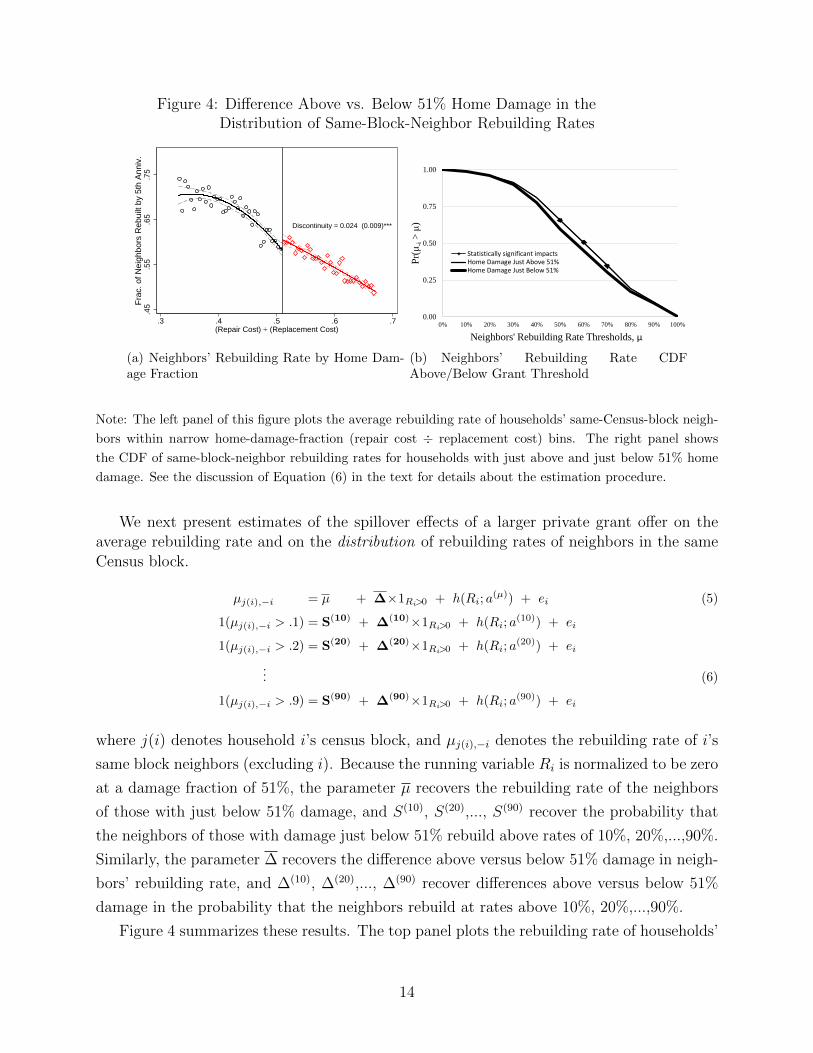
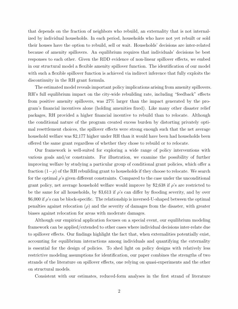
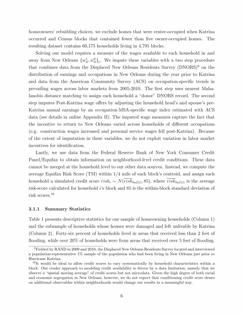
Figure 4: Difference Above vs. Below 51% Home Damage in theDistribution of Same-Block-Neighbor Rebuilding Rates

Discontinuity = 0.024 (0.009)***

.45

.55

.65

.75

Fra

c. o

f Nei

ghbo

rs R

ebui

lt by

5th

Ann

iv.


(a) Neighbors’ Rebuilding Rate by Home Dam-age Fraction

DATA MOMENTS:

1

0

1

MODEL MOMENTS:

1

0

0.3004

0.17

0.0884

0

0.00

0.25

0.50

0.75

1.00

0% 10% 20% 30% 40% 50% 60% 70% 80% 90% 100%

Pr(

μ-i >

μ)

Neighbors' Rebuilding Rate Thresholds, μ

Statistically significant impactsHome Damage Just Above 51%Home Damage Just Below 51%

0

0.25

0.5

0.75

1

0% 10% 20% 30% 40% 50% 60% 70% 80% 90% 100%

Pr(

μ-i >

μ)

Home Damage Just Above 51% (Model)Home Damage Just Above 51% (Data)Home Damage Just Below 51% (Model)Home Damage Just Below 51% (Data)

-0.025

0

0.025

0.05

0.075

Δ(y) Δ Δ(10) Δ(20) Δ(30) Δ(40) Δ(50) Δ(60) Δ(70) Δ(80) Δ(90)

Dis

con

tin

uit

y i

n P

r(μ

-i>

μ)

Data Model

(b) Neighbors’ Rebuilding Rate CDFAbove/Below Grant Threshold

Note: The left panel of this figure plots the average rebuilding rate of households’ same-Census-block neigh-

bors within narrow home-damage-fraction (repair cost ÷ replacement cost) bins. The right panel shows

the CDF of same-block-neighbor rebuilding rates for households with just above and just below 51% home

damage. See the discussion of Equation (6) in the text for details about the estimation procedure.

We next present estimates of the spillover effects of a larger private grant offer on theaverage rebuilding rate and on the distribution of rebuilding rates of neighbors in the sameCensus block.

µj(i),−i = µ + ∆×1Ri>0 + h(Ri; a(µ)) + ei (5)

1(µj(i),−i > .1) = S(10) + ∆(10)×1Ri>0 + h(Ri; a(10)) + ei

1(µj(i),−i > .2) = S(20) + ∆(20)×1Ri>0 + h(Ri; a(20)) + ei

... (6)

1(µj(i),−i > .9) = S(90) + ∆(90)×1Ri>0 + h(Ri; a(90)) + ei

where j(i) denotes household i’s census block, and µj(i),−i denotes the rebuilding rate of i’s

same block neighbors (excluding i). Because the running variable Ri is normalized to be zero

at a damage fraction of 51%, the parameter µ recovers the rebuilding rate of the neighbors

of those with just below 51% damage, and S(10), S(20),..., S(90) recover the probability that

the neighbors of those with damage just below 51% rebuild above rates of 10%, 20%,...,90%.

Similarly, the parameter ∆ recovers the difference above versus below 51% damage in neigh-

bors’ rebuilding rate, and ∆(10), ∆(20),..., ∆(90) recover differences above versus below 51%

damage in the probability that the neighbors rebuild at rates above 10%, 20%,...,90%.

Figure 4 summarizes these results. The top panel plots the rebuilding rate of households’

14

same-block neighbors within narrow damage fraction bins, which jumps by 2.4 percentage

at the 51% damage grant threshold. The bottom panel plots the neighbors’ rebuilding

rate “survival” functions for households with just below 51% damage (constructed from the

estimates of S(10),..., S(90)) and just above 51% damage (S(10) + ∆(10),..., S(90) + ∆(90)). The

relatively steep slope over a wide range of rebuilding rates implies that the grant discontinuity

quasi-experiment occurred on blocks with a wide range of “baseline” rebuilding rates. A

comparison of the plots for households with above and below 51% damage reveals that

spillover effects operated primarily by pushing some blocks that would have experienced

rebuilding below the rates of 50%, 60%, and 70% to above these rates. This pattern suggests

that an exogenous shock to rebuilding has a large effect on amenity values in areas with

baseline rebuilding rates near this range and a relatively small effect on amenity values

in areas with very low baseline rebuilding rates. Appendix Table A2 shows robustness to

alternative specifications.

3.3 From RDD to a Model

To achieve the main goals of this paper, we need to go beyond RDD and build a model. The

first goal is to evaluate the welfare impact of the RH program, which requires the ability

to infer quantitatively households’ preferences from their observed choices. In particular, to

evaluate RH’s choice-based subsidy structure, we need to compare the gains from the amenity

spillover relative to the losses for marginal households whose choices were distorted by the

subsidies. The second and more important goal is to provide information for future policy

designs, which involves comparing equilibrium impacts of various counterfactual policies.

Prediction of these impacts requires a solid understanding of households’ choices and the

interaction among households, which, in turn, requires knowledge of the fundamental factors

underlying the observed outcomes. In addition, counterfactual policy analyses, being out-

of-sample predictions, involve extrapolations that call for a structural model.

RDD analyses provide two clear messages that are instrumental for us to make some of

the key modeling choices. The first message is that spillovers significantly exist in the data,

which suggests that a model ignoring spillovers might have misleading policy implications.

Therefore, although it involves more modeling, an equilibrium approach, rather than a single

agent decision framework, is necessary. The second message is that spillovers are likely to

be highly nonlinear. Based on these findings, we build an equilibrium model of neighbors’

choices in the presence of amenity spillovers, and allow for a very flexible specification of the

spillover function.

15

4 Model

Displaced households (homeowners) make dynamic decisions about moving back to (and

rebuilding) their pre-Katrina homes. In every period, a household that has not moved back

or sold its property can choose to 1) move back and rebuild, or 2) sell the property, or 3)

wait until the next period. Each household’s decision potentially influences the block’s at-

tractiveness, a spillover effect that is not internalized by individual households. The model

incorporates the following factors that influence a household’s net payoff from rebuilding: (i)

the cost of home repairs relative to other non-repair options, (ii) household’s labor market

opportunities in and out of New Orleans, (iii) the strength of the household’s idiosyncratic

attachment to the neighborhood, (iv) the exogenous state of the neighborhood (e.g., flood

damages, infrastructure repairs and unobserved amenities), and (v) the influence of neigh-

bors’ rebuilding choices on the attractiveness of the neighborhood.

4.1 Primitives

There are J communities/blocks; and each block is the setting of an equilibrium.16 There

are I households living in different communities. Let j(i) be the block where household i

owns its home, and Ij be the set of households living in j. Hurricane Katrina occurs at time

t = 0. Each household lives forever but has the option to rebuild each period only from 1 to

T = 5, where each period is one year. Households differ in their housing-related costs, labor

market opportunities, levels of attachment to their community and accesses to credit. All

information is public among neighbors but is only partially observed by the researcher.17

4.1.1 Monetary Incentives

Housing-Related Costs Several housing-related costs and prices influence the financial

consequences of each of the three options: 1) i’s remaining mortgage balance when Katrina

occurred (Mi ≥ 0); 2) the cost/value of the pre-Katrina physical structure of i’s house (psi )

(superscript s for structure); 3) the cost of repairing/restoring the house from it’s damaged

state (ki ≤ psi ); 4) the (endogenous) market value of the property (the damaged house and

16We choose to focus on the equilibrium within each block in order to achieve a more detailed understandingof interactions and spillovers among neighbors. An alternative modeling framework would treat a larger unit,e.g., the whole region, as one economy. Relative to our framework, the second framework may provide abroader view, but most likely at the cost of abstracting from some of the micro features we consider in orderto remain tractable.

17Given that households in our model are neighbors, we have assumed a complete information structure.The main predictions from our model would still hold if one assumes incomplete information among neighbors.Regardless of the model’s information structure, however, it is reasonable to allow for and hence importantto account for factors that are common knowledge to the households but are unobservable to the researcher.

16

the land) if sold privately pi, 5) the value of insurance payments received (insi ≤ ki); and 6)

the additional incentives created by RH.

If household i has yet to rebuild entering period t, the household may return and reside

on the block in period t by paying a one-time repair cost ki at the beginning of period t,

i.e., within a year.18 Households who rebuild are reimbursed for uninsured damages by a

RH (option 1) grant G1i = min($150,000, ki−insi). Reflecting RH’s slow rollout, grants are

dispersed at the start of t = 3 if repairs occurred earlier and are dispersed at the time repairs

occur otherwise.

For each period that it resides away from its pre-Katrina block, a household rents ac-

commodation comparable to its pre-Katrina home at a cost of renti = δ× psi , where δ is the

user cost of housing. The household can sell its property either through RH (option 2) for

a price G2,i or privately for a price pi. The private sales price, as we specify later, depends

on the replacement cost of the structure (psi ), its damage (ki), neighborhood characteristics,

and the neighborhood’s rebuilding rate µj.

Labor Market Opportunities Household i faces different wages in New Orleans {w1it}t ,

and outside of New Orleans {w0it}t . The two vectors of wages differ across households, which

is another source of variation that may lead to different choices across households.

4.1.2 Household Preferences

A household derives utility from consumption (c), neighborhood amenities, and an idiosyn-

cratic taste for a place. The values of the last two components are normalized to zero for the

outside option. The (relative) value of amenities in community j consists of an exogenous

part aj and an endogenous part that depends on the fraction (µjt) of neighbors who have

rebuilt.19 Households differ in their attachment to their community (ηi), which stands for

their private non-pecuniary incentives to return home, assumed to follow an i.i.d. N(0, σ2

η

).

18For simplicity, we assume that rebuilding occurs during the same period (year) that the rebuilding costis paid. This assumption should be realistic in the vast majority of cases, as 92% of residential constructionstarts are completed within one year, and the median time to completion is under six months (Census Surveyof Construction, 2005-2010).

19Presumably spillover effects can operate via channels that are more general than the rebuilding rateor the fraction of agents who take relevant actions. For feasibility reasons, the literature has typicallyabstracted away from more general spillover effects. For example, in Bayer and Timmins (2005), the fractionof neighbors taking the relevant action enters individuals utility linearly. We make a weaker assumption byallowing household utility to be a much more flexible function of the rebuilding rate.

17

Household i’s per-period utility v (·) , suppressing its dependence on (c, a, η) , is given by,

vit(µj(i),t; dit) =

ln(cit) if dit < 1

ln(cit) + aj(i) + g(µj(i),t) + ηi if dit = 1,(7)

where dit = 1 if household i has chosen to rebuild by period t, dit = −1 if i has sold its house

by time t, and dit = 0 if neither is true. µj(i),t ∈ [0, 1] is the fraction of neighbors who have

rebuilt by time t, and g(µ) is a non-decreasing function governing the amenity spillovers.20

Notice that dit represents one’s status at time t; one’s action at time t is reflected by

a change in dit relative to dit−1. We assume that both selling and rebuilding are absorbing

states and hence the only feasible changes in dit over time are 0→ 1 or 0→ −1. Therefore,

dit > dit−1 is equivalent to rebuilding in period t; and dit < dit−1 is equivalent to selling in

period t.21

4.1.3 Intertemporal Budget Constraint/Financing Constraints

Letting 1 (·) be the indicator function, the household intertemporal budget constraint is

given by, }cit = 1

(dit=1

)×w1

i + 1(dit<1

)×w0

i labor earnings}− 1

(dit<1

)×renti − 1

(dit>−1

)×mortgageit flow housing costs

− 1(dit>di,t−1

)×ki

+ 1(di3 =1 and t=3

)×G1i repair costs/reimbursements

+ 1(dit>dit−1 and t>3

)×G1i }

+ 1(dit<dit−1)×max(G2i, pi

)home sale proceeds}

+ Ait − Ait+1

/Rt change in asset holding.

The first line gives one’s labor income. The second line is the flow housing cost, which equals

the rent cost if one lives outside of the city plus the mortgage payment if the household still

owns its home. The next line is the one-time repair cost one incurs if one rebuilds in this

20A non-decreasing spillover function rules out the possibility of particularly strong “congestion” effects,which we view as reasonable in our framework as the number of residents is not allowed to exceed thepre-disaster equilibrium level.

21Fewer than 4% of households repaired and then sold their home later during the sample period.

18

period (dit > dit−1) . The next two lines summarize the grant one gets for rebuilding, reflecting

the fact that the RH grants were typically paid out more than two years after Katrina. The

second last line represents the event of a household selling its property (dit < dit−1) to RH

or privately, whichever gives a higher price. Finally, the household can also change its asset

holding at interest rate Rt, with the restriction that,

Ait ≥

0 if riski < ρ∗

−∞ if riski ≥ ρ∗,

where riski is household i’s Equifax Risk Score (TM). Only households with risk scores above

ρ∗ may borrow to finance home repairs.22

Property Sales Price The price at which a household can sell its home privately pi is

endogenous and affected by the equilibrium neighborhood rebuilding status, such that

ln (pi) = P(psi , ki, zj(i), µj(i),T

)+ εi.

The function P (·) captures physical and amenity values of the house. The physical value

depends on the house’s pre-Katrina physical structure cost (psi ) and its damage status cap-

tured by ki. The amenity value depends on both exogenous observable block characteristics

vector zj(i) and the endogenous block rebuilding rate(µj(i),T

). We use the final rebuilding

rate µj(i),T as a determinant of the price to capture the idea that house buyers are forward

looking and care about the future amenity in the neighborhood. The last term εi is idiosyn-

cratic and known to the household, which may be correlated with other unobservables such

as block amenities and individual tastes.

4.2 Household Problem

Given the fraction of households who have rebuilt by the end of t − 1 and the endogenous

law of motion for future rebuilding rates (Γjt(µ)) , the discounted value of remaining lifetime

22The assumption that households with risk scores above ρ∗ have unlimited credit access is less restrictivethan it might seem. In our framework, the rebuilding decision is the only major investment choice thathouseholds face, so the meaningful assumption is that “unconstrained” households have sufficient credit tofinance home repairs/rebuilding.

19

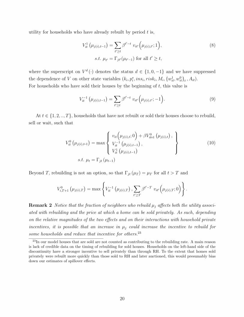
utility for households who have already rebuilt by period t is,

V 1it

(µj(i),t−1

)=∑t′≥t

βt′−t vit′

(µj(i),t′ ; 1

), (8)

s.t. µt′ = Γjt′(µt′−1) for all t′ ≥ t,

where the superscript on V d (·) denotes the status d ∈ {1, 0,−1} and we have suppressed

the dependence of V on other state variables (ki, psi , insi, riski,Mi, {w1

it, w0it}t , Ait).

For households who have sold their houses by the beginning of t, this value is

V −1it

(µj(i),t−1

)=∑t′≥t

βt′−t vit′

(µj(i),t′ ;−1

). (9)

At t ∈ {1, 2, .., T}, households that have not rebuilt or sold their houses choose to rebuild,

sell or wait, such that

V 0it

(µj(i),t−1

)= max

vit

(µj(i),t; 0

)+ βV 0

it+1

(µj(i),t

),

V −1it

(µj(i),t−1

),

V 1it

(µj(i),t−1

) (10)

s.t. µt = Γjt (µt−1)

Beyond T, rebuilding is not an option, so that Γjt (µT ) = µT for all t > T and

V 0i,T+1

(µj(i),T

)= max

{V −1it

(µj(i),T

),∑t′≥T

βt′−T vit′

(µj(i),T ; 0

)}.

Remark 2 Notice that the fraction of neighbors who rebuild µj affects both the utility associ-

ated with rebuilding and the price at which a home can be sold privately. As such, depending

on the relative magnitudes of the two effects and on their interactions with household private

incentives, it is possible that an increase in µj could increase the incentive to rebuild for

some households and reduce that incentive for others.23

23In our model houses that are sold are not counted as contributing to the rebuilding rate. A main reasonis lack of credible data on the timing of rebuilding for sold houses. Households on the left-hand side of thediscontinuity have a stronger incentive to sell privately than through RH. To the extent that homes soldprivately were rebuilt more quickly than those sold to RH and later auctioned, this would presumably biasdown our estimates of spillover effects.

20

4.3 Equilibrium

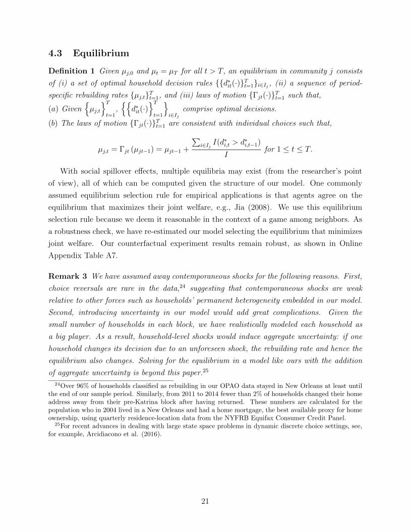
Definition 1 Given µj,0 and µt = µT for all t > T, an equilibrium in community j consists

of (i) a set of optimal household decision rules {{d∗it(·)}Tt=1}i∈Ij , (ii) a sequence of period-

specific rebuilding rates {µj,t}Tt=1, and (iii) laws of motion {Γjt(·)}Tt=1 such that,

(a) Given{µj,t

}Tt=1

,{{

d∗it(·)}Tt=1

}i∈Ij

comprise optimal decisions.

(b) The laws of motion {Γjt(·)}Tt=1 are consistent with individual choices such that,

µj,t = Γjt (µjt−1) = µjt−1 +

∑i∈Ij I(d∗i,t > d∗i,t−1)

Ifor 1 ≤ t ≤ T.

With social spillover effects, multiple equilibria may exist (from the researcher’s point

of view), all of which can be computed given the structure of our model. One commonly

assumed equilibrium selection rule for empirical applications is that agents agree on the

equilibrium that maximizes their joint welfare, e.g., Jia (2008). We use this equilibrium

selection rule because we deem it reasonable in the context of a game among neighbors. As

a robustness check, we have re-estimated our model selecting the equilibrium that minimizes

joint welfare. Our counterfactual experiment results remain robust, as shown in Online

Appendix Table A7.

Remark 3 We have assumed away contemporaneous shocks for the following reasons. First,

choice reversals are rare in the data,24 suggesting that contemporaneous shocks are weak

relative to other forces such as households’ permanent heterogeneity embedded in our model.

Second, introducing uncertainty in our model would add great complications. Given the

small number of households in each block, we have realistically modeled each household as

a big player. As a result, household-level shocks would induce aggregate uncertainty: if one

household changes its decision due to an unforeseen shock, the rebuilding rate and hence the

equilibrium also changes. Solving for the equilibrium in a model like ours with the addition

of aggregate uncertainty is beyond this paper.25

24Over 96% of households classified as rebuilding in our OPAO data stayed in New Orleans at least untilthe end of our sample period. Similarly, from 2011 to 2014 fewer than 2% of households changed their homeaddress away from their pre-Katrina block after having returned. These numbers are calculated for thepopulation who in 2004 lived in a New Orleans and had a home mortgage, the best available proxy for homeownership, using quarterly residence-location data from the NYFRB Equifax Consumer Credit Panel.

25For recent advances in dealing with large state space problems in dynamic discrete choice settings, see,for example, Arcidiacono et al. (2016).

21

4.3.1 Tipping

Viewing a problem from an equilibrium perspective not only involves a different modeling

framework than an individual decision model, it also bears important policy implications.

We discuss one of these implications, the possibility of “tipping” in the presence of multiple

equilibria. Even though agents agree on the equilibrium that maximizes their joint welfare

given the set of possible equilibria, there can still be room for policy interventions because

policies can affect the equilibrium set. For example, a policy change may introduce a new

equilibrium with a higher rebuilding rate that would not have been self-consistent otherwise,

i.e., a “tipping” phenomenon, as illustrated in online Appendix I.

In many cases, it is both convenient and perhaps reasonable for researchers to approx-

imate an outcome variable as a smooth function of explanatory variables. With “tipping”

being a potential event, this approach may no longer be appropriate, because when “tip-

ping” happens, there will necessarily be a “jump” in the equilibrium outcomes. Modifying

the smooth function by adding certain discontinuity points may help if one knows the lo-

cations (e.g., combinations of community characteristics and policies) and the magnitude

of these jumps, however, such information is usually not available when performing ex ante

policy evaluations. Our framework lends itself toward obtaining such knowledge by explicitly

modeling and solving for the equilibrium.

4.4 Further Empirical Specifications

Going from RDD to a model requires assumptions, some of which have been discussed above.

The following describes our parametric specifications of two other important components of

the model.

4.4.1 Exogenous Neighborhood Amenities

The exogenous component of block-specific amenity values are not directly observable to the

researcher, and are modeled as

aj(i) = z′j(i),tγ + bj(i),

where z′j(i),tγ captures heterogeneity in amenity values across blocks based on pre-determined

block observable characteristics (z), including flood exposure, pre-Katrina demographic com-

position, and a linear time trend to capture city-wide improvements in infrastructure.26

bj ∼ N (0, σ2b ) captures heterogeneity in block amenity values unobservable to the researcher.

26We have also estimated a more flexible model, where time trends are allowed to vary by block-levelflooding severity. The fit and policy implications of this more flexible model, as presented in the onlineappendix, are similar to those of the original (more parsimonious) model.

22

4.4.2 Amenity Spillovers

The amenity spillover function, which characterizes the impact of the block rebuilding rate

on the block’s amenity value, is given by

g(µ) = S × Λ(µ;λ),

where the parameter S measures the total change in amenity utility associated with a block

transitioning from a 0% rebuilding rate to a 100% rebuilding rate. Λ : [0, 1] → [0, 1] is

the Beta cumulative distribution function, with parameters λ = [λ1, λ2]′ . The Beta CDF

is a parsimonious but flexible function that allows for a wide range of spillover patterns,

illustrated in online appendix Figure A5. The parameter λ2 governs the function’s shape,

and λ1 governs the location of the strongest marginal spillovers.

5 Model Estimation

5.1 Parameters Estimated outside of the Model

To reduce computational burden, we estimate the home price offer function outside of the

model, with the following form

ln (pi) = P1

(psi , ki, zj(i)

)+ P2(µ−i,j(i),T ) + εi,

where P1() is a flexible function with polynomials and interactions and P2() is a linear spline.

OLS estimates of this equation are likely to be biased for several reasons. First, µ−i,j(i),T

is likely to be correlated with the residual εi, because unobserved block amenities bj(i) that

directly affect offered home prices should also affect neighbors’ rebuilding choices. Second,

offered prices are only observed for households who choose to sell, which will cause selection

bias if idiosyncratic household attachment ηi is correlated with unobserved house traits εi.

We use fixed effects χτ(i) for Census tracts, a larger unit of geography nesting Census

blocks, to control for unobserved block amenities, where τ(i) denotes the Census tract house-

hold i belonged to. This approach controls for unobservable factors affecting house prices

that are common within a tract. We account for selection using the Heckman (1979) two-

step procedure. We use the RH grant formula discontinuity as the excluded instrument in

a first stage probit predicting the probability of a home sale,27 and include the associated

27A non-parametric selection-correction using a polynomial in the estimated “propensity score” (salei) asa control function yields nearly identical results.

23

inverse Mills ratio as a regressor in the second stage estimating equation, such that

ln (pi) = P1

(psi , ki, zj(i)

)+ P2(µj(i),T ) + ρλ(Φ−1(salei)) + χτ(i) + ei. (11)

5.2 Parameters Estimated within the Model

The vector of structural parameters (Θ) to be estimated within the model consists of the

parameters governing: 1) the dispersion of household attachment (ση) , 2) the exogenous

block-specific amenity values (γ, σb) , 3) the nature of amenity spillovers (S, λ) , and 4) the

credit score threshold for borrowing (ρ∗) . The estimation is via indirect inference, which

consists of two steps. Step 1 computes from the data a set of “auxiliary models” that sum-

marize the patterns in the data to be targeted for the structural estimation. Step 2 repeatedly

simulates data with the structural model, computes corresponding auxiliary models using

the simulated data, and searches for model parameters that match the simulated auxiliary

models with those in Step 1.

5.2.1 Auxiliary Models

The auxiliary models that we target include:

1. RDD estimates of the private rebuilding elasticity: y and ∆(y) from equation (3) char-

acterizing the left and right limits of the private rebuilding rate at the 51% damage grant

threshold.

2. RDD estimates of spillovers from private rebuilding choices onto neighbors’ rebuilding

choices: µ and ∆ from Equation (5) characterizing the left and right limits of a household’s

neighbors’ rebuilding rate at the 51% damage grant threshold, and µ(p) and ∆(p) from equa-

tions (6) for p = 10, 20, ..., 90 characterizing the left and right limits of the likelihood that

a household’s neighbors’ rebuilding rate exceeds each threshold at the 51% damage grant

threshold.

3. Descriptive regressions of year t private rebuilding indicators on block flood exposure and

average block credit scores for t=1,...,5.

5.2.2 Estimation Algorithm

Our estimation algorithm involves an outer loop searching over the space of structural pa-

rameters, and an inner loop computing model-generated auxiliary models.

The Inner Loop With simulated data, computing auxiliary models follows the same pro-

cedure as described above. We focus on describing the solution to the model. Given Θ, for

24

each community j observed in the data, simulate N copies of communities jn that share the

same observable characteristics but differ in unobservables, at both the individual and the

community level. The unobservables are drawn from the distributions governed by (ση, σb) .

For each simulated community, solve for the equilibrium as follows, where we suppressing

the block subscript j.

1. For each block, locate all possible “self-consistent” period T block rebuilding rates: for

each nT = 1, ..., I, compute the offer price for each household pi = P(psi , ki, zj(i), µj,T = nT/I

),

count the number of simulated households n∗T (nT ; Θ) who prefer to rebuild when µ∗j,T = nT/I,

which is self consistent if n∗T (nT ; Θ) = nT .

2. Select the self-consistent µj,T that maximizes total block welfare WT−1 =∑

i Vi,T−1. Store

the associated offer price for each household.

3. Taking equilibrium home prices as given, locate all possible “self-consistent” period T − 1

block rebuilding rates: for each nT−1 = 1, ..., I, count the number of simulated block house-

holds n∗T−1(nT ; Θ) who prefer to rebuild when µ∗j,T−1 = nT/I, which is self consistent if

n∗T−1(nT−1; Θ) = nT−1.

4. Select the self-consistent µj,T−1 that maximizes total block welfare WT−1 =∑

i Vi,T−1.

5. Repeat steps 3 and 4 for t = T−2, T−3, ..., 1.

The Outer Loop Let β denote our chosen set of auxiliary model parameters computed

from data. Let β(Θ) denote the corresponding auxiliary model parameters obtained from

simulating datasets from the model (parameterized by a particular vector Θ) and computing

the same estimators. The structural parameter estimator is the solution

Θ = argminΘ [β(Θ)− β]′W [β(Θ)− β],

where W is a weighting matrix. We obtain standard errors for β(Θ) by numerically com-

puting ∂Θ/∂β and applying the delta method to the variance-covariance matrix of β. We

augment the indirect inference strategy with an importance sampling technique suggested

by Sauer and Taber (2012) that ensures a smooth objective function.

5.3 Identification

Although all of the structural parameters are identified jointly, we provide a sketch of iden-

tification here by describing which auxiliary models are most informative about certain

structural parameters. More details can be found in the appendix.

25

5.3.1 ση, σb, and g(µ)

The logic follows three steps for identifying parameters governing the unobserved heterogene-

ity in households’ payoffs (η, b, and g(µ)). First, identifying the dispersion of η + b + g(µ).

The elasticity of rebuilding with respect to private financial incentives is governed primarily

by the dispersion of unobserved heterogeneity in preferences for rebuilding across all house-

holds. A household’s own rebuilding decision follows a threshold rule based on whether

or not η + b + g(µ) exceeds a particular value.28 All else equal, rebuilding choices will be

less price-elastic if unobserved heterogeneity is more disperse, because any given change in

the utility threshold for rebuilding caused by a change in financial incentives sweeps over a

smaller fraction of unobserved heterogeneity. The dispersion of η+ b+g(µ) is thus identified

mainly from the size of RDD parameter ∆y, the difference between the rebuilding rates of

households with damage levels just above versus below the RH grant formula discontinuity,

relative to the change in incentives ∆cost across the grant threshold.29

Second, identifying the distribution of idiosyncratic heterogeneity, characterized by ση,

separately from the distribution of block-level heterogeneity, characterized by σb and g(µ).

The relative variance of idiosyncratic and block-level heterogeneity governs the dispersion of

rebuilding rates across blocks. If the variance of(b+g(µ)

)is small, unobserved heterogeneity

in payoffs will be mostly idiosyncratic to households within blocks, and blocks with similar

observable fundamentals will experience similar rebuilding rates (i.e. µj will have a relatively

small variance conditional on observables). If the variance of(b+g(µ)

)is large, there will be

large differences between blocks with similar observable fundamentals in the average payoff

to rebuilding, and µj will have a larger variance conditional on observables. The variance of

η (i.e. ση) is thus separately identified from the variance of(b+g(µ)

)mainly by the auxiliary

model parameters S(10), S(20), ..., S(90) measuring the CDF of block rebuilding rates among

28For example, a household would prefer to rebuild in period 5 versus not rebuilding if,

bj(i) + ηi +

(1− ββ5 − β9

)g(µj(i),5) >

(1− ββ5 − β9

)max{cit}

(8∑t=1

ln cit

∣∣∣does not rebuild

)

−

[(1− ββ5 − β9

)max{cit}

(8∑t=1

ln cit

∣∣∣rebuild at t=5

)+ Z ′j(i)tγ

]

29In principle, variation in other financial incentives like private insurance settlements, the market valuesof households’ properties, and the prevailing wages in post-Katrina New Orleans in household members’ pre-Katrina occupations could aid in identification. We rely, instead, on the RD variation in financial incentivesfor identification, because we expect that differences across households in these other financial incentivesto be correlated with households’ idiosyncratic attachment to home and/or the unobserved amenities inhouseholds’ neighborhoods. On the other hand, while households with damages on either side of the RHgrant formula threshold faced significantly different incentives to rebuild, they faced similar distributions ofη and b.

26

household in a particular pre-determined circumstance.

Third, identifying the spillover function g(µ) separately from the distribution of exoge-

nous block-level amenities b. The spillover function g(µ) governs the effect of one household

rebuilding on its neighbors’ incentive to rebuild, and hence the extent to which private

incentives will generate spillover effects. A private incentive for particular households to

rebuild will have larger spillover effects on the choices of neighbors when g(µ) is steeper.

These spillover effects will only occur on blocks where the damage levels are within partic-

ular ranges (not necessarily connected) if g(.) is sufficiently nonlinear, while spillovers will

occur similarly across all blocks if g(.) is approximately linear. The identification challenge

is that unobserved group-level variables such as b also cause neighbors to behave similarly,

so inferring spillover effects in this way is invalid if households’ financial incentives are cor-

related with b. We solve this identification challenge by exploiting the variation in financial

incentives generated by the RH grant discontinuity, variation which is as-good-as random

and thus orthogonal to b. 30

In particular, the amplitude and shape of a general non-decreasing smooth amenity

spillover function g(µ) are identified by spillovers from the discontinuously higher RH grant

offers made to households with damages just above versus just below the RH grant formula

threshold (∆, ∆(10),..., ∆(90)), compared to the direct effect of those higher grant offers on

private rebuilding choices (∆y). Under our parameterization of the amenity spillover func-

tion, g(µ;S, λ1, λ2), the amplitude of g(µ) is governed by the parameter S, and the shape of

g(µ) is governed by the parameters λ1 and λ2. The average spillover measure ∆ is therefore

particularly informative about the value of S, and the pattern of spillovers onto the prob-

abilities that neighbors’ rebuilding rates exceed the different thresholds (∆(10), ..., ∆(90)) is

particularly informative about the values of the shape parameters λ1 and λ2.

Given functional form assumptions, our parameterized model is technically identifiable

via moments describing the correlation between neighbors’ choices that do not have a causal

interpretation without the RDD. However, if identified entirely off functional forms, the

model is at higher risk of attributing correlation between neighbors’ choices caused by a

common effect (bj) to spillovers or vice versa. The RH formula discontinuity provides

exogenous variation that shifts individual households’ incentives but is uncorrelated with

neighborhood-level unobservables (bj), which serves as a more reliable way to disentangle

the role of neighborhood-level unobservables from causal spillover effects (g(µj)) within the

range of variation in the data. The model identified as such gives us more confidence in its

policy implications.

30See Online Appendix V for a more formal presentaion of this argument.

27

5.3.2 Other Parameters

The credit risk cutoff parameter ρ∗ determines the fraction of households in each neighbor-

hood who are borrowing constrained. Because most RH grants were paid more than two

years after Hurricane Katrina, the prevalence of borrowing constraints strongly influences

the predicted timing of rebuilding. For households who were borrowing constrained, the

self-financing of home repairs prior to RH grants being disbursed would have entailed a

significant reduction to lifetime consumption utility, forcing them to delay rebuilding. For

households who were able to borrow, consumption would be smooth across periods regardless

of the timing of repairs. The parameter ρ∗ is thus mainly identified by the extent to which

the repair rate hazard increased after the disbursement of RH grants across neighborhoods

with different mean Equifax risk scores.

Finally, the parameters γ describing exogenous differences in amenity values across flood

categories are identified by differences in rebuilding rates across flood categories beyond what

would be predicted by households’ private incentives.

6 Results

6.1 Parameter Estimates

The top panel of Table 3 presents the estimated parameters governing the spillover function.

To illustrate the spillover effects, we plot the estimated spillover function g(µ) in the left panel

of Figure 5. Fully rebuilding a block increases its flow amenity valuation by the equivalent

of a 43 log-point increase in annual non-housing consumption. However, the incremental

impact of additional rebuilding depends critically on the block’s initial rebuilding rate. The

marginal impact of rebuilding on a block’s amenity value is close to zero in areas with

rebuilding rates below 50%; yet it is substantial in areas with rebuilding rates above 50%.

The right panel of Figure 5 plots the estimated effect of a block’s rebuilding rate on house

offer prices, i.e., the spline in µ−i from estimating equation (11). A home’s price increases

by nearly 20% if all of the homes on its block are rebuilt (µ−i = 1 relative to µ−i = 0).

The marginal impact of rebuilding on home prices is the highest in areas with the highest

rebuilding rate.

The next panels of Table 3 characterize the exogenous components of block amenities.

An estimated set of year-specific utility intercepts increases monotonically with time, pre-

sumably reflecting city-wide infrastructure repairs. Coefficient estimates on flood exposure

do not exhibit a clear pattern, suggesting that a block’s amenity value is not strongly cor-

related with its flooding risk per se. We find significant heterogeneity in the unobserved

28

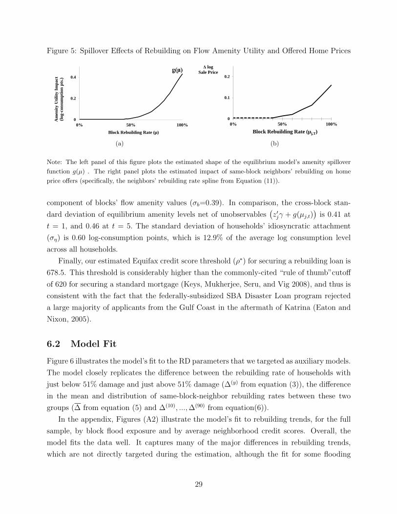
Figure 5: Spillover Effects of Rebuilding on Flow Amenity Utility and Offered Home Prices

0%

0.1

0.11

0.12

0.13

0

0.2

0.4

0% 50% 100%

Block Rebuilding Rate (µ)

Am

enit

y U

tili

ty I

mp

act

(lo

g-c

on

sum

pti

on

pts

.)

(a)

0

0.1

0.2

0% 50% 100%

Block Rebuilding Rate (µj,T)

Δ log Sale Price

(b)

Note: The left panel of this figure plots the estimated shape of the equilibrium model’s amenity spillover

function g(µ) . The right panel plots the estimated impact of same-block neighbors’ rebuilding on home

price offers (specifically, the neighbors’ rebuilding rate spline from Equation (11)).

component of blocks’ flow amenity values (σb=0.39). In comparison, the cross-block stan-

dard deviation of equilibrium amenity levels net of unobservables(z′jγ + g(µj,t)

)is 0.41 at

t = 1, and 0.46 at t = 5. The standard deviation of households’ idiosyncratic attachment

(ση) is 0.60 log-consumption points, which is 12.9% of the average log consumption level

across all households.

Finally, our estimated Equifax credit score threshold (ρ∗) for securing a rebuilding loan is

678.5. This threshold is considerably higher than the commonly-cited “rule of thumb”cutoff

of 620 for securing a standard mortgage (Keys, Mukherjee, Seru, and Vig 2008), and thus is

consistent with the fact that the federally-subsidized SBA Disaster Loan program rejected

a large majority of applicants from the Gulf Coast in the aftermath of Katrina (Eaton and

Nixon, 2005).

6.2 Model Fit

Figure 6 illustrates the model’s fit to the RD parameters that we targeted as auxiliary models.

The model closely replicates the difference between the rebuilding rate of households with

just below 51% damage and just above 51% damage (∆(y) from equation (3)), the difference

in the mean and distribution of same-block-neighbor rebuilding rates between these two

groups (∆ from equation (5) and ∆(10), ...,∆(90) from equation(6)).

In the appendix, Figures (A2) illustrate the model’s fit to rebuilding trends, for the full

sample, by block flood exposure and by average neighborhood credit scores. Overall, the

model fits the data well. It captures many of the major differences in rebuilding trends,

which are not directly targeted during the estimation, although the fit for some flooding

29

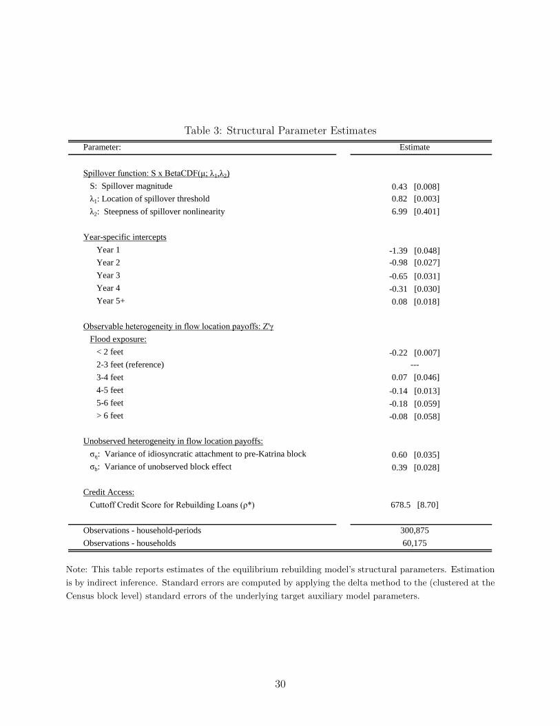
Table 3: Structural Parameter Estimates

Parameter: Estimate

Spillover function: S x BetaCDF(μ; λ1,λ2)

S: Spillover magnitude 0.43 [0.008]

λ1: Location of spillover threshold 0.82 [0.003]

λ2: Steepness of spillover nonlinearity 6.99 [0.401]

Year-specific intercepts

Year 1 -1.39 [0.048]

Year 2 -0.98 [0.027]

Year 3 -0.65 [0.031]

Year 4 -0.31 [0.030]

Year 5+ 0.08 [0.018]

Observable heterogeneity in flow location payoffs: Z'γ

Flood exposure:

< 2 feet -0.22 [0.007]

2-3 feet (reference) ---

3-4 feet 0.07 [0.046]

4-5 feet -0.14 [0.013]

5-6 feet -0.18 [0.059]

> 6 feet -0.08 [0.058]

Unobserved heterogeneity in flow location payoffs:

ση: Variance of idiosyncratic attachment to pre-Katrina block 0.60 [0.035]

σb: Variance of unobserved block effect 0.39 [0.028]

Credit Access:

Cuttoff Credit Score for Rebuilding Loans (ρ*) 678.5 [8.70]

Observations - household-periods 300,875

Observations - households 60,175

Note: This table reports estimates of the equilibrium rebuilding model’s structural parameters. Estimation

is by indirect inference. Standard errors are computed by applying the delta method to the (clustered at the

Census block level) standard errors of the underlying target auxiliary model parameters.

30

Figure 6: Goodness of Fit: Actual and Model-Predicted R.D. “Spillover” Coefficients

DATA MOMENTS:

1

0

1

MODEL MOMENTS:

1

0

0.3004

0.17

0.0884

0

0.00

0.25

0.50

0.75

1.00

0% 10% 20% 30% 40% 50% 60% 70% 80% 90% 100%

Pr(

μ-i >

μ)

Neighbors' Rebuilding Rate Thresholds, μ

Statistically significant impactsHome Damage Just Above 51%Home Damage Just Below 51%

0

0.25

0.5

0.75

1

0% 10% 20% 30% 40% 50% 60% 70% 80% 90% 100%

Pr(

μ-i >

μ)

Home Damage Just Above 51% (Model)Home Damage Just Above 51% (Data)Home Damage Just Below 51% (Model)Home Damage Just Below 51% (Data)

-0.025

0

0.025

0.05

0.075

Δ(y) Δ Δ(10) Δ(20) Δ(30) Δ(40) Δ(50) Δ(60) Δ(70) Δ(80) Δ(90)

Dis

con

tin

uit

y i

n P

r(μ

-i>

μ)

Data Model

categories is not as good. Figure A3 shows that the model fits well to the distribution

of block rebuilding rates five years after Katrina. Table A3 shows the model’s fit to the

rebuilding rates of subgroups within finer subgroups, none of which are targeted moments.

7 Counterfactual Policy Simulations

We use the estimated equilibrium model to perform three sets of counterfactual policy anal-

yses that shed light on the optimal structure of disaster relief grants. The first quantifies

spillover effects by decomposing the full impacts of RH into its impact via private financial

incentives alone and that via amenity spillovers. The second illustrates how policy impli-

cations can change once equilibrium interactions are accounted for, by contrasting welfare

effects of RH with those under unconditional grants. In the appendix we also present results

of a policy that eliminates the discontinuity in the RH formula so that grant becomes a

continuous function of damages. Finally, we illustrate how our modeling framework can be

used for optimal policy designs.

7.1 RH’s Direct Effects and Feedback Effects

To measure the importance of the “feedback” effects from amenity spillovers, we compare the

full equilibrium impact of RH with the impact generated by the program’s financial incentives

alone (holding amenities fixed). To begin, we simulate equilibrium rebuilding choices without

RH grants. We then simulate the impact of introducing RH’s financial incentives while

holding amenity values fixed, which boils down to an individual decision model without

31

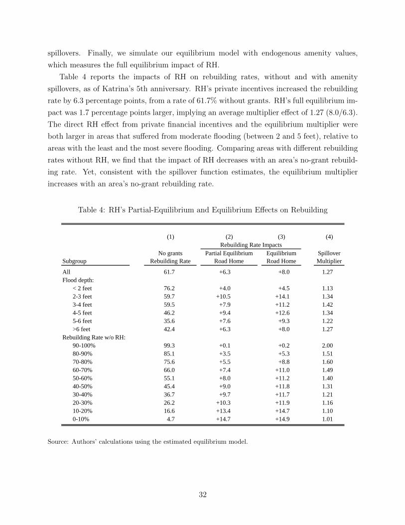
spillovers. Finally, we simulate our equilibrium model with endogenous amenity values,

which measures the full equilibrium impact of RH.

Table 4 reports the impacts of RH on rebuilding rates, without and with amenity

spillovers, as of Katrina’s 5th anniversary. RH’s private incentives increased the rebuilding

rate by 6.3 percentage points, from a rate of 61.7% without grants. RH’s full equilibrium im-

pact was 1.7 percentage points larger, implying an average multiplier effect of 1.27 (8.0/6.3).

The direct RH effect from private financial incentives and the equilibrium multiplier were

both larger in areas that suffered from moderate flooding (between 2 and 5 feet), relative to

areas with the least and the most severe flooding. Comparing areas with different rebuilding

rates without RH, we find that the impact of RH decreases with an area’s no-grant rebuild-

ing rate. Yet, consistent with the spillover function estimates, the equilibrium multiplier

increases with an area’s no-grant rebuilding rate.

Table 4: RH’s Partial-Equilibrium and Equilibrium Effects on Rebuilding

(1) (2) (3) (4)

Subgroup

Unconditional

Grants (UG)

Rebuilding Rate

Partial Equilibrium

Road Home

Equilibrium

Road Home

Spillover

Multiplier

All 60.6 +7.3 +9.1 1.25

Flood depth:

< 2 feet 75.9 +4.3 +4.8 1.12

2-3 feet 58.1 +11.8 +15.7 1.33

3-4 feet 57.3 +9.7 +13.4 1.38

4-5 feet 44.0 +11.3 +14.8 1.31

5-6 feet 33.9 +9.1 +11.0 1.21

>6 feet 40.7 +7.8 +9.7 1.24

Rebuilding Rate under UG:

90-100% 99.3 +0.1 +0.2 2.00

80-90% 84.6 +3.9 +5.8 1.49

70-80% 74.5 +6.3 +9.9 1.57

60-70% 64.2 +8.7 +12.8 1.47

50-60% 53.5 +9.3 +12.8 1.38

40-50% 43.6 +10.6 +13.6 1.28

30-40% 34.6 +11.6 +13.8 1.19

20-30% 24.7 +11.8 +13.4 1.14

10-20% 14.8 +15.1 +16.5 1.09

0-10% 2.7 +16.6 +16.9 1.02

(1) (2) (3) (4)

Subgroup

No grants

Rebuilding Rate

Partial Equilibrium

Road Home

Equilibrium

Road Home

Spillover

Multiplier

All 61.7 +6.3 +8.0 1.27

Flood depth:

< 2 feet 76.2 +4.0 +4.5 1.13

2-3 feet 59.7 +10.5 +14.1 1.34

3-4 feet 59.5 +7.9 +11.2 1.42

4-5 feet 46.2 +9.4 +12.6 1.34

5-6 feet 35.6 +7.6 +9.3 1.22

>6 feet 42.4 +6.3 +8.0 1.27

Rebuilding Rate w/o RH:

90-100% 99.3 +0.1 +0.2 2.00

80-90% 85.1 +3.5 +5.3 1.51

70-80% 75.6 +5.5 +8.8 1.60

60-70% 66.0 +7.4 +11.0 1.49

50-60% 55.1 +8.0 +11.2 1.40

40-50% 45.4 +9.0 +11.8 1.31

30-40% 36.7 +9.7 +11.7 1.21

20-30% 26.2 +10.3 +11.9 1.16

10-20% 16.6 +13.4 +14.7 1.10

0-10% 4.7 +14.7 +14.9 1.01

Rebuilding Rate Impacts

Rebuilding Rates by Policy

Source: Authors’ calculations using the estimated equilibrium model.

32

7.1.1 Potential Multiple Equilibria and Policy Implications

As mentioned earlier, even though households agree on the equilibrium to be selected given

the set of possible equilibria, policy interventions can affect the equilibrium set. As a result,

impacts of a given policy may vary substantially across blocks, depending on the nature of

each block’s equilibrium set without the policy and the degrees to which these sets vary with

the policy. Our framework is well-suited to study such implications, because it allows us to

calculate the full set of equilibria under any given policy.

We start with relating block characteristics to the nature of their equilibrium sets. We

divide blocks into two groups based on equilibrium uniqueness. Group 1 accounts for 86%

of blocks, all of which have a unique equilibrium with and without RH. Group 2 consists

of all the other blocks, i.e., those with multiple equilibria in at least one case. As shown in

Panel A of Table 5, relative to Group 1 blocks, Group 2 blocks are more likely to have been

exposed to more severe flooding, to have higher fractions of households that are black, with

lower than college education and/or lower credit scores. In other words, multiple equilibria

are more likely to exist in more disadvantaged blocks.

Next, we contrast RH impacts between the two groups, as shown in Panels B and C of

Table 5. Consistent with Group 2 being more disadvantaged, the average rebuilding rate

would have been lower in Group 2 (58%) than in Group 1 (62%) without RH; and RH’s

financial incentive alone increased the rebuilding rate more for Group 2 (8.7%) than for

Group 1 (5.9%). Consistent with “tipping”, RH generated a much larger multiplier effect for

Group 2 in the presence of multiple equilibria. As a result, RH’s full equilibrium impact was

much higher for Group 2 (16.6% on rebuilding rate and $8,600 on welfare) than for Group 1

(6.3% on rebuilding rate and $630 on welfare). Thanks to multiple equilibria, RH was more

effective where help was needed the most, i.e., more disadvantaged blocks.

7.2 Welfare Effects of RH versus Unconditional Grants

The RH grant program discouraged households from relocating by requiring relocating house-

holds to give their properties to a state land trust. Compared to unconditional transfers,

conditional transfers entail an efficiency loss or “excess burden” for households whose choices

are distorted by the conditions associated with the transfer. However, when considered in

an equilibrium framework with spillovers, the conditional nature of the RH transfer may im-

prove total welfare if the value of the positive externality generated by RH-induced rebuilding

exceeds the private losses from the program’s distortion.

To study the welfare consequences of RH’s conditional structure, we compare the RH

equilibrium outcomes with those under an unconditional grant program that pays a grant

33

computed with the RH rebuilding grant formula to all households regardless of their choices.

We compute the equivalent variation (EV RHi ) necessary to make a household’s equilibrium

welfare under the unconditional grant policy equal to that under RH, which measures house-

holds’ utility difference under the two policies in dollars.31 To account for the difference in

subsidies granted in two programs, we compute household-level net welfare impacts(dWRH

i

)by subtracting the change in program costs, i.e.,

dWRHi = EV RH

i − (Granti,RH −Granti,Uncond). (12)

Table 6 summarizes the results. Column (1) reports that 9.1% of households were

“marginal” in the sense that their rebuilding choices under RH differed from what they

would have made under the unconditional grant policy. This fraction was the smallest in the

least flooded areas and highest in moderately flooded areas. The next three columns show

the net welfare impacts of RH relative to the unconditional grant(dWRH

i

)for inframarginal,

marginal and all households, respectively. For an average inframarginal household, welfare

improved by $4,950 as the result of the conditional grant structure that induced positive

spillovers from the rebuilding of marginal households. An average marginal household, how-

ever, was worse off by an equivalent of $24,360. Overall, RH increased average household

welfare by $2,177 ($131M in total), relative to the unconditional grant policy. Except for ar-

eas with 5-6 feet of flooding, where a $475 loss occurred, welfare improved across areas with

different flooding exposures. The improvement was particularly significant in moderately

flooded areas, which is consistent with our previous finding that RH’s impacts on rebuilding

rates were larger in these areas.

Remark 4 Our calculation of dWRHi does not take into account the value of properties

turned over to the state by RH relocation grant recipients. Before Katrina, the total value of

the land on which these properties sat (appraised by the parish Assessor’s Office for property

tax purposes) was $54M. Assigning this value to the properties in the welfare calculation

would increase the calculated per capita “government savings” from RH compared to the

unconditional grant program by $908 (=$54M / 60,175). While we do not have reliable data

on the post-Katrina value of these properties, we expect the value to be substantially lower

31Specifically, we find the dollar amount that when paid as a constant per-period flow from t = 1, ..., Tunder the unconditional grant policy provides household i the same discounted lifetime utility i receives inequilibrium under RH. Letting evi denote the per-period payment, our equivalent variation measure EVi isthe present discounted value of this stream,

EVi =

(evir

)(1− 1

(1 + r)T+1

)

34

Table 5: Neighborhood Traits, Rebuilding Rate Impacts, and Welfare Impacts by Numberof Equilibria

A. Neighborhood Charactoristics

Group 1:Unique

Group 2:Multiple

Pre-Katrina block flood exposure:< 2 feet 51 162 - 3 feet 10 243 - 4 feet 9 234 - 5 feet 9 145 - 6 feet 7 3> 6 feet 14 19

Demographic composition:Percent black (Census block) 55 67Percent college educated (Census tract) 52 47

Equifax risk score (spatial moving average):<600 18 22600-625 16 21625-650 17 17650-675 14 15675-700 13 6700-725 10 8>725 12 10

Percent of replicated blocks 84.0 16.0

B. RH Rebuilding Impacts

No grants Rebuilding Rate 62.1 58.0

Partial Eqm. RH Impact +5.9 +8.7

Equilibrium RH Impact +6.3 +16.6

Multiplier 1.07 1.92

C. RH Welfare Impacts

Equilibrium RH Impact (per capita) $627 $8,602

than $54M, because the properties are located disproportionately in areas of the city that

received heavy flooding and in the neighborhoods that were slowest to rebuild.

7.3 The Optimal Generosity of Relocation Grants

We have shown that RH improved average household welfare by $2,177 relative to an uncon-

ditional grant policy. In the following, we examine the potential for further improvements by

35

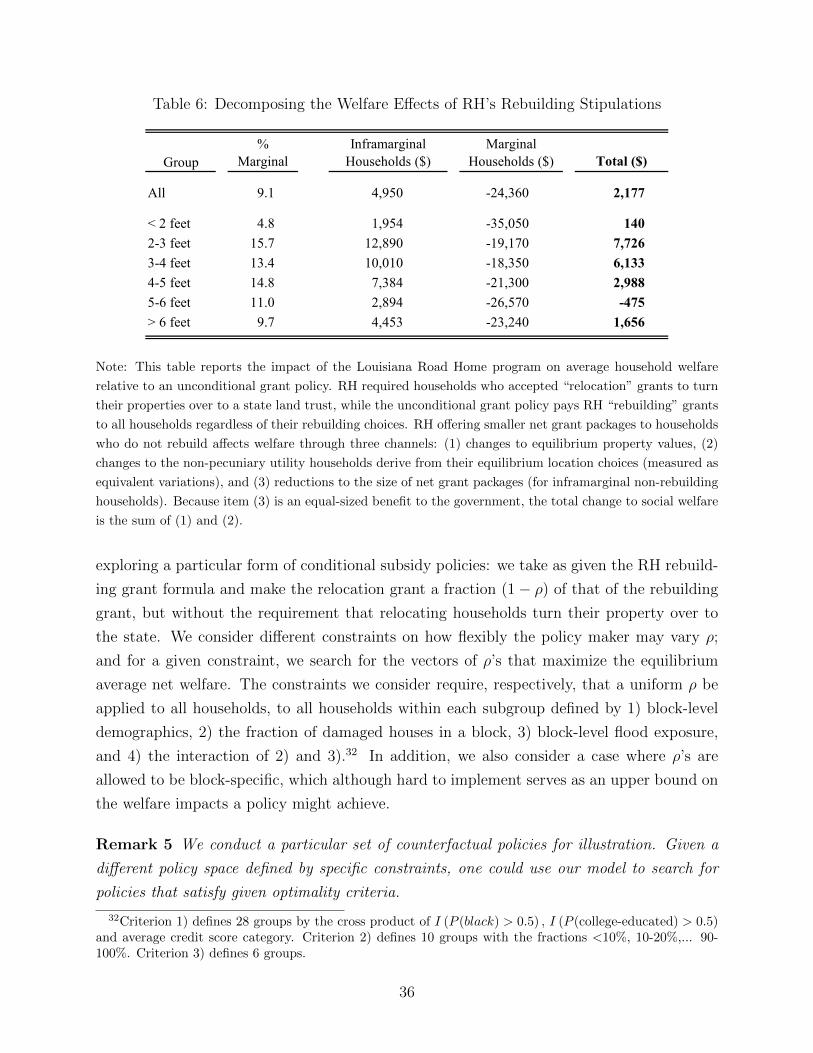
Table 6: Decomposing the Welfare Effects of RH’s Rebuilding Stipulations

Group%

MarginalInframarginal

Households ($)Marginal

Households ($) Total ($)

All 9.1 4,950 -24,360 2,177

< 2 feet 4.8 1,954 -35,050 140

2-3 feet 15.7 12,890 -19,170 7,726

3-4 feet 13.4 10,010 -18,350 6,133

4-5 feet 14.8 7,384 -21,300 2,988

5-6 feet 11.0 2,894 -26,570 -475

> 6 feet 9.7 4,453 -23,240 1,656

Note: This table reports the impact of the Louisiana Road Home program on average household welfare

relative to an unconditional grant policy. RH required households who accepted “relocation” grants to turn

their properties over to a state land trust, while the unconditional grant policy pays RH “rebuilding” grants

to all households regardless of their rebuilding choices. RH offering smaller net grant packages to households

who do not rebuild affects welfare through three channels: (1) changes to equilibrium property values, (2)

changes to the non-pecuniary utility households derive from their equilibrium location choices (measured as

equivalent variations), and (3) reductions to the size of net grant packages (for inframarginal non-rebuilding

households). Because item (3) is an equal-sized benefit to the government, the total change to social welfare

is the sum of (1) and (2).

exploring a particular form of conditional subsidy policies: we take as given the RH rebuild-

ing grant formula and make the relocation grant a fraction (1− ρ) of that of the rebuilding

grant, but without the requirement that relocating households turn their property over to

the state. We consider different constraints on how flexibly the policy maker may vary ρ;

and for a given constraint, we search for the vectors of ρ’s that maximize the equilibrium

average net welfare. The constraints we consider require, respectively, that a uniform ρ be

applied to all households, to all households within each subgroup defined by 1) block-level

demographics, 2) the fraction of damaged houses in a block, 3) block-level flood exposure,

and 4) the interaction of 2) and 3).32 In addition, we also consider a case where ρ’s are

allowed to be block-specific, which although hard to implement serves as an upper bound on

the welfare impacts a policy might achieve.

Remark 5 We conduct a particular set of counterfactual policies for illustration. Given a

different policy space defined by specific constraints, one could use our model to search for

policies that satisfy given optimality criteria.

32Criterion 1) defines 28 groups by the cross product of I (P (black) > 0.5) , I (P (college-educated) > 0.5)and average credit score category. Criterion 2) defines 10 groups with the fractions <10%, 10-20%,... 90-100%. Criterion 3) defines 6 groups.

36

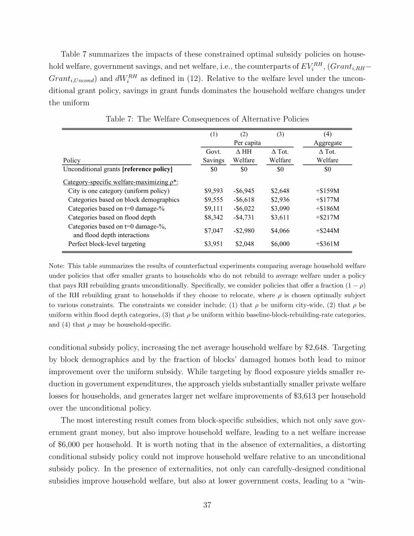
Table 7 summarizes the impacts of these constrained optimal subsidy policies on house-

hold welfare, government savings, and net welfare, i.e., the counterparts of EV RHi , (Granti,RH−

Granti,Uncond) and dWRHi as defined in (12). Relative to the welfare level under the uncon-

ditional grant policy, savings in grant funds dominates the household welfare changes under

the uniform

Table 7: The Welfare Consequences of Alternative Policies

(1) (2) (3) (4)Aggregate

PolicyGovt.

SavingsΔ HH

WelfareΔ Tot.

WelfareΔ Tot.

WelfareUnconditional grants [reference policy] $0 $0 $0 $0

Category-specific welfare-maximizing ρ*: City is one category (uniform policy) $9,593 -$6,945 $2,648 +$159M Categories based on block demographics $9,555 -$6,618 $2,936 +$177M Categories based on t=0 damage-% $9,111 -$6,022 $3,090 +$186M Categories based on flood depth $8,342 -$4,731 $3,611 +$217M Categories based on t=0 damage-%, and flood depth interactions

$7,047 -$2,980 $4,066 +$244M

Perfect block-level targeting $3,951 $2,048 $6,000 +$361M

Per capita

Note: This table summarizes the results of counterfactual experiments comparing average household welfare

under policies that offer smaller grants to households who do not rebuild to average welfare under a policy

that pays RH rebuilding grants unconditionally. Specifically, we consider policies that offer a fraction (1− ρ)

of the RH rebuilding grant to households if they choose to relocate, where ρ is chosen optimally subject

to various constraints. The constraints we consider include; (1) that ρ be uniform city-wide, (2) that ρ be

uniform within flood depth categories, (3) that ρ be uniform within baseline-block-rebuilding-rate categories,

and (4) that ρ may be household-specific.

conditional subsidy policy, increasing the net average household welfare by $2,648. Targeting

by block demographics and by the fraction of blocks’ damaged homes both lead to minor

improvement over the uniform subsidy. While targeting by flood exposure yields smaller re-

duction in government expenditures, the approach yields substantially smaller private welfare

losses for households, and generates larger net welfare improvements of $3,613 per household

over the unconditional policy.

The most interesting result comes from block-specific subsidies, which not only save gov-

ernment grant money, but also improve household welfare, leading to a net welfare increase

of $6,000 per household. It is worth noting that in the absence of externalities, a distorting

conditional subsidy policy could not improve household welfare relative to an unconditional

subsidy policy. In the presence of externalities, not only can carefully-designed conditional

subsidies improve household welfare, but also at lower government costs, leading to a “win-

37

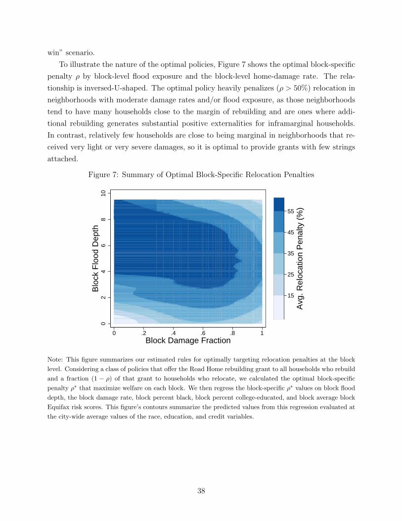
win” scenario.

To illustrate the nature of the optimal policies, Figure 7 shows the optimal block-specific

penalty ρ by block-level flood exposure and the block-level home-damage rate. The rela-

tionship is inversed-U-shaped. The optimal policy heavily penalizes (ρ > 50%) relocation in

neighborhoods with moderate damage rates and/or flood exposure, as those neighborhoods

tend to have many households close to the margin of rebuilding and are ones where addi-

tional rebuilding generates substantial positive externalities for inframarginal households.

In contrast, relatively few households are close to being marginal in neighborhoods that re-

ceived very light or very severe damages, so it is optimal to provide grants with few strings

attached.

Figure 7: Summary of Optimal Block-Specific Relocation Penalties

02

46

810

Blo

ck F

lood

Dep

th

0 .2 .4 .6 .8 1Block Damage Fraction

15

25

35

45

55

Avg

. Rel

ocat

ion

Pen

alty

(%

)

Note: This figure summarizes our estimated rules for optimally targeting relocation penalties at the block

level. Considering a class of policies that offer the Road Home rebuilding grant to all households who rebuild

and a fraction (1 − ρ) of that grant to households who relocate, we calculated the optimal block-specific

penalty ρ∗ that maximize welfare on each block. We then regress the block-specific ρ∗ values on block flood

depth, the block damage rate, block percent black, block percent college-educated, and block average block

Equifax risk scores. This figure’s contours summarize the predicted values from this regression evaluated at

the city-wide average values of the race, education, and credit variables.

38

8 Conclusion

Many housing policies are predicated on the idea that housing investments generate positive

externalities. The optimal design of these policies requires an understanding of the nature

of these externalities, the decision making processes of individual households, and the way

those decisions intertwine in equilibrium. Toward that end, we have developed a frame-

work that combines the strength of quasi-experimental research designs and the strength

of structural equilibrium modeling. We have applied this framework to the case of post-

Katrina reconstruction. The quasi-experimental variation in private financial incentives that

we exploit for identification admits a causal interpretation of both the direct effects of RH

financial incentives on rebuilding and of the spillover effects of those incentives onto neigh-

bors’ rebuilding choices. Our equilibrium model replicates these internally-consistent causal

relationships and other patterns not directly targeted for identification.

We have found that rebuilding caused economically important amenity spillovers: the

distorting RH program led to higher welfare compared to an unconditional subsidy policy. We

have illustrated how our framework can inform the design of optimal subsidy policies, which

further improve household welfare while saving government costs, compared to unconditional

subsidies. Such a “win-win” situation would be an implausible prediction if researchers were

to treat household decisions in isolation.

Although our empirical application focuses on a special event and a particular source of

identifying variation, our equilibrium modeling framework for studying private investment

choices in equilibrium can be applied/extended to other cases where individual decisions are

inter-related due to spillover effects. Our strategy for identifying such models using quasi-

experimental variation is also promising for studies that aim at shedding light on policy

designs with relatively less restrictive modeling assumptions for identification.

Several extensions to our framework are worth pursuing. The first one is to embed our

model into a more general equilibrium framework that considers equilibrium interactions

within an entire city or region. A more general framework would also model equilibrium in

the labor market, allowing for the possibility of downward sloping local labor demand (e.g.,

Albouy 2009, Roback 1982) conditional on population and the possibility that changes to

the size of the local population shifts the local labor demand curve. Identifying these more

general equilibrium models, however, would require data from multiple markets. A related

but different extension would examine another dimension of policy impact heterogeneity, one

that differs across different types of block geographies (Jacobs, 1961).

Another extension is to incorporate other spatially-biased policies and consider them

simultaneously with the rebuilding grant policy. The existence of other distortive policies

39

may lead to situations where the number of households living in certain areas is inefficiently

high prior to a disaster occurring. This could happen due to, for example, moral hazard

resulting from the precedent of generous post-disaster bailouts (Gregory 2014) or the federal

income tax code’s relatively favorable treatment of less productive places (Albouy 2009, Colas

and Hutchinson 2015). Although existing estimates of these distortive effects are relatively

small compared to the direct incentives for locating in particular cities and neighborhoods

following some disasters, optimal rebuilding grant policies may differ depending on whether

or not these other existing distortions are accounted for.

References

[1] Albouy, David. 2009. “The Unequal Geographic Burden of Federal Taxation.” Journal

of Political Economy 117(4):635-667.

[2] Anenberg, Elliot and Edward Kung. forthcoming. “Estimates of the Size and Source of

Price Declines Due to Nearby Foreclosures.” American Economic Review.

[3] Autor, David, Christopher Palmer, and Parag Pathak. forthcoming. “Externalities from

Rent Control? Evidence from Cambridge MA.” Journal of Political Economy.

[4] Bayer, P., F. Ferreira, and R. McMillan. 2007. “A Unified Framework for Measuring

Preferences for Schools and Neighborhoods,” Journal of Political Economy, 115(4)588-

638.

[5] Bayer, P., R. McMillan, and K. Reuben. 2005. “Resedential Segregation in General

Equilibrium,” NBER Working Paper 11095.

[6] Bayer, Patrick and Christopher Timmins. 2007. “Estimating Equilibrium Models of

Sorting Across Locations.” Economic Journal, 117(518): 353-374.

[7] Bayer, Patrick and Christopher Timmins. 2005. “On the equilibrium properties of loca-

tional sorting models.” Journal of Urban Economics, 57(3): 462-477.

[8] Bayer, Patrick and Christopher Timmins. 2007. “Estimating Equilibrium Models of

Sorting Across Locations.” Economic Journal, 117(518): 353-374.

[9] Bajari, Patrick, C. Lanier Benkard and Jonathan Levin. 2007. “Estimating Dynamic

Models of Imperfect Competition.” Econometrica, 75(5): 1331–1370.

[10] Bajari, Patrick, Han Hong, John Krainer and Denis Nekipelov. 2010. “Estimating Static

Models of Strategic Interactions.” Journal of Business and Economic Statistics, 28(4):

469-482.

40

[11] Berry, Steven, James Levinsohn and Ariel Pakes. 1995. “Automobile Prices in Market

Equilibrium.” Econometrica, 63(4): 841-890.

[12] Bjorn, P., and Q. Vuong. 1984. “Simultaneous Equations Models for Dummy Endoge-

nous Variables: A Game Theoretic Formulation With Application to Labor Force Par-

ticipation.” SSWP 537, California Institute of Technology.

[13] Blume, Lawrence, William Brock, Steven Durlauf, and Yannis Ioannides. 2010. “Iden-

tification of Social Interactions, ”in Handbook of Social Economics, J. Benhabib, A.

Bisin, and M. Jackson, eds., Amsterdam: North Holland.

[14] Bresnahan, Timothy and Peter Reiss. 1990. “Entry in Monopoly Markets.” The Review

of Economic Studies, 57: 531-553.

[15] Brock, William and Steven Durlauf. 2001. “Discrete Choice with Social Interactions,”

Review of Economic Studies, 68: 235-260.

[16] Brock, William and Steven Durlauf. 2006. Multinomial Choice with Social Interac-

tions,Ein The Economy as an Evolving Complex System, L. Blume and S. Durlauf, eds.,

New York: Oxford University Press.

[17] Brock, William and Steven Durlauf. 2007. “Identification of Binary Choice Models with

Social Interactions,” Journal of Econometrics, 140(1), 52-75.

[18] Calononico, Sebastian, Matias Catteneo, and Rocio Titiunik. 2014. “Robust Nonpara-

metric Confidence Intervals for Regression Discontinuity Designs.” Econometrica, 82(6):

2295-2326.

[19] Campbell, John Y., Stefano Giglio, and Parag Pathak. 2011. “Forced Sales and House

Prices.” American Economic Review.

[20] Ciliberto, Federico and Elie Tamer. 2009. “Market Structure and Multiple Equilibria in

Airline Markets.” Econometrica, 77(6): 1791-1828.

[21] Das, Mitali, Whitney Newey, and Francis Vella. 2003. “Nonparametric Estimation of

Sample Selection Models.” Review of Economic Studies, 70(1): 33-58.

[22] de Paula, Aureo. 2009. “Inference in a Synchronization Game with Social Interactions,”

Jornal of Econometrics, 148(1):56-71.

[23] de Paula, Aureo. 2013. “Econometric Analysis of Games with Multiple Equilibria.”

Annual Review of Economics, 5: 107-131.

41

[24] Einav, L. 2010. “Not All Rivals Look Alike: Estimating an Equilibrium Model of the

Release Date Timing Game.” Economic Inquiry, 48(2): 369–390.

[25] Elliott, J. R. and J. Pais. 2006. “Race, class, and Hurricane Katrina: Social differences

in human responses to disaster.” Social Science Research 35(2):295-321.

[26] Epple, D., T. Romer, and H. Sieg. 2001. “Interjurisdictional Sorting and Majority Rule:

An Empirical Analysis,” Econometrica, 69: 1437E465.

[27] Epple, D. and H. Sieg. 1999. “Estimating Equilibrium Models of Local Jurisdictions,”

Journal of Political Economy, 107: 645E81.

[28] Gregory, J. 2012. “The Impact of Rebuilding Grants and Wage Subsidies on the Reset-

tlement Choices of Hurricane Katrina Victims,” Working Paper

[29] Groen, J. A. and A. E. Polivka. 2009. “Going Home after Hurricane Katrina: Determi-

nants of Return Migration and Changes in Affected Areas.” Demography 47(4):821-844.

[30] Guerrieri, Veronica, Daniel Hartley, and Erik Hurst. 2013. “Endogenous Gentrification

and Housing Price Dynamics.” Journal of Public Economics, 100:45-60.

[31] Harding, John P. , Eric Rosenblatt, and Vincent W. Yao. 2009. “The Contagion Effect

of Foreclosed Properties.” Journal of Urban Economics, 66: 164-178.

[32] Ioannides, Y. and J. Zabel. 2008. “Interactions, Neighborhood Selection, and Housing

Demand,” Journal of Urban Economics, 63: 229-252.

[33] Ioannides, Yannis M. 2003. “Interactive Property Valuations.” Journal of Urban Eco-

nomics, 53: 145-170.

[34] Jacobs, Jane. 1961. “The death and life of great American cities.” Random House.

[35] Jia, Panle. 2008. “What Happens When Wal-Mart Comes to Town: An Empirical

Analysis of the Discount Retailing Industry.” Econometrica, 76: 1263–1316.

[36] Manski, C. 1993. “Identification of Endogenous Social Effects: The Reflection Problem,”

The Review of Economic Studies, 60: 531-542

[37] McCarthy, K. D.J. Peterson, N. Sastry, and M. Pollard. 2006. “The Repopulation of

New Orleans After Hurricane Katrina.” Technical report. RAND Corp.

42

[38] Keys, Benjamin, Tanmoy Mukherjee, Amit Seru, and Vikrant Vig. 2008. “Securitiza-

tion and Screening: Evidence from Subprime Mortgage Backed Securities.” Quarterly

Journal of Economics, 125(1).

[39] Paxson, C. and C. Rouse. 2008. “Returning to New Orleans after Hurricane Katrina.”

American Economic Review, 98(2):38-42.

[40] Roback, J. 1982. “Wages, Rents, and the Quality of Life.” The Journal of Political

Economy 90(6):1257-1278.

[41] Rossi-Hansberg Sarte Owens. 2010. “Housing Externalities.” Journal of Political Econ-

omy, 118(3):485-535.

[42] Sauer, R and C. Taber. 2017. “Importance sampling in indirect inference.” NBER Work-

ing Paper No. 23669.

[43] Tamer, Elie. 2003. “Incomplete Simultaneous Discrete Response Model with Multiple

Equilibria.” The Review of Economic Studies, 70(1): 147-165.

[44] Todd, P. and K. Wolpin. 2008. “Ex Ante Evaluation of Social Programs,” Annals of

Economics and Statistics, 91/92: 263-291

[45] U.S. Census Bureau’s Survey of Construction (2005, 2006, 2007, 2008, 2009, 2010).

[46] Vigdor, J. 2008. “The Economic Aftermath of Hurricane Katrina.” The Journal of

Economic Perspectives 22:135-154.

[47] Vigdor, J. L. 2007. “The Katrina Effect: Was There a Bright Side to the Evacuation of

Greater New Orleans?” The B.E. Journal of Economic Analysis & Policy 7(1).

[48] Zissimopoulos, J. and L. Karoly. 2010. “Employment and Self-Employment in the Wake

of Hurricane Katrina.” Demography 47(2):345-356.

Appendix I. Illustration of “Tipping”

Figure A1 illustrates the phenomenon of “tipping.” The top panel of Figure A1 plots a hypothetical private

demand schedule for rebuilding evaluated at the amenity level associated with a 0% rebuilding rate and the

actual marginal benefit curve.33 Self-consistent rebuilding rates are the zeros of the latter curve. Tipping

33The private demand curve is downward sloping by definition as it is simply a highest-to-lowest orderingof individual households’ net benefits to rebuilding. The actual marginal benefit curve incorporates eachadditional household’s positive contribution to block amenities and can thus be downward or upward sloping.

43

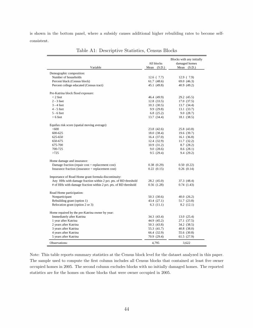
is shown in the bottom panel, where a subsidy causes additional higher rebuilding rates to become self-

consistent.

Table A1: Descriptive Statistics, Census Blocks

All blocks

Blocks with any initially

damaged homes

Variable Mean (S.D.) Mean (S.D.)

Demographic composition:

Number of households 12.6 ( 7.7) 12.9 ( 7.9)

Percent black (Census block) 61.7 (48.6) 69.0 (46.3)

Percent college educated (Census tract) 45.1 (49.8) 40.9 (49.2)

Pre-Katrina block flood exposure:

< 2 feet 46.4 (49.9) 29.2 (45.5)

2 - 3 feet 12.8 (33.5) 17.0 (37.5)

3 - 4 feet 10.3 (30.5) 13.7 (34.4)

4 - 5 feet 9.9 (29.8) 13.1 (33.7)

5 - 6 feet 6.8 (25.2) 9.0 (28.7)

> 6 feet 13.7 (34.4) 18.1 (38.5)

Equifax risk score (spatial moving average):

<600 23.8 (42.6) 25.8 (43.8)

600-625 18.0 (38.4) 19.6 (39.7)

625-650 16.4 (37.0) 16.1 (36.8)

650-675 12.4 (32.9) 11.7 (32.2)

675-700 10.9 (31.2) 8.7 (28.2)

700-725 9.0 (28.6) 8.6 (28.1)

>725 9.5 (29.4) 9.4 (29.2)

Home damage and insurance:

Damage fraction (repair cost ÷ replacement cost) 0.38 (0.29) 0.50 (0.22)

Insurance fraction (insurance ÷ replacement cost) 0.22 (0.15) 0.26 (0.14)

Importance of Road Home grant formula discontinuity:

Any HHs with damage fraction within 2 pct. pts. of RD threshold 28.2 (45.0) 37.3 (48.4)

# of HHs with damage fraction within 2 pct. pts. of RD threshold 0.56 (1.28) 0.74 (1.43)

Road Home participation:

Nonparticipant 50.3 (30.6) 40.0 (26.2)

Rebuilding grant (option 1) 43.4 (27.1) 51.7 (23.8)

Relocation grant (option 2 or 3) 6.3 (11.1) 8.2 (12.1)

Home repaired by the pre-Katrina owner by year:

Immediately after Katrina 34.3 (43.4) 13.0 (25.4)

1 year after Katrina 44.9 (45.2) 27.1 (37.5)

2 years after Katrina 50.3 (43.8) 34.2 (38.5)




Observations: 4,795 3,622

Note: This table reports summary statistics at the Census block level for the dataset analyzed in this paper.

The sample used to compute the first column includes all Census blocks that contained at least five owner

occupied homes in 2005. The second column excludes blocks with no initially damaged homes. The reported

statistics are for the homes on those blocks that were owner occupied in 2005.

44

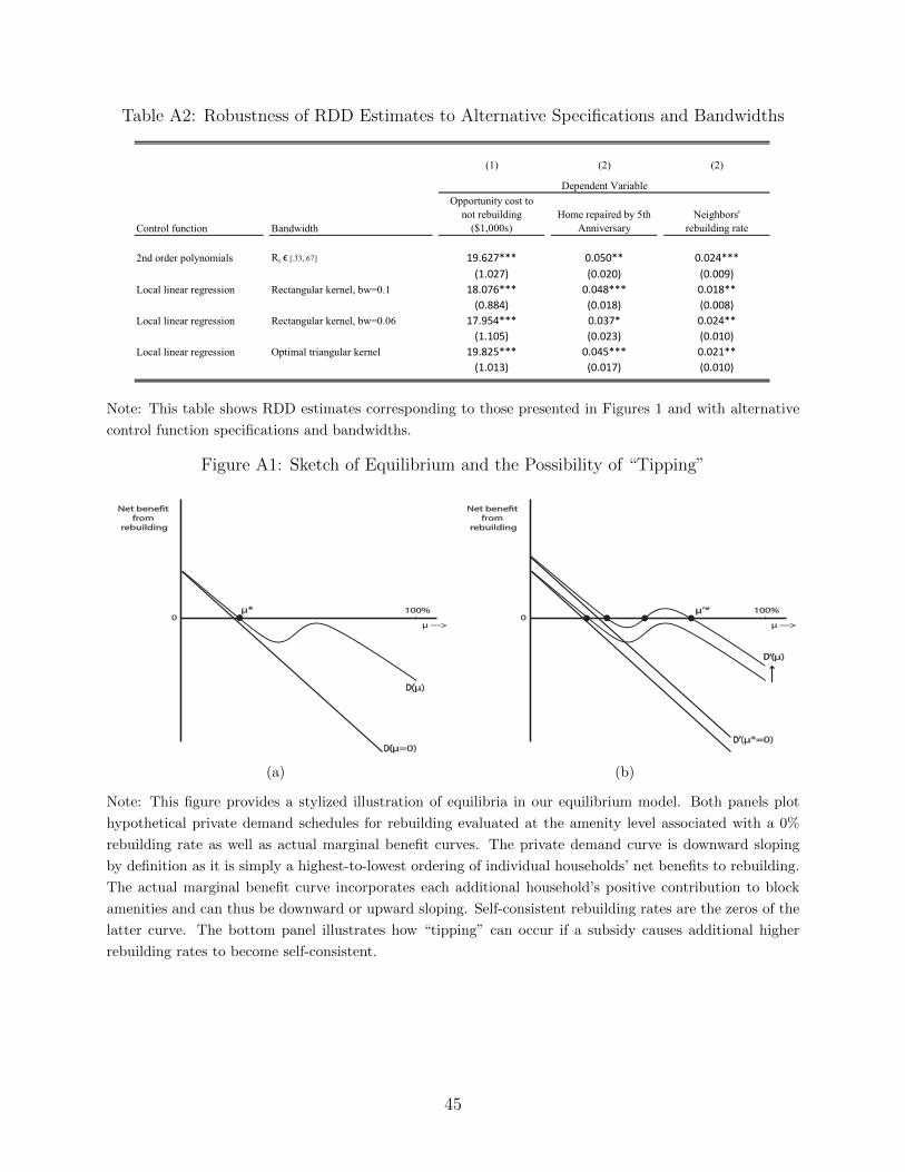
Table A2: Robustness of RDD Estimates to Alternative Specifications and Bandwidths

(1) (2) (2)

Control function Bandwidth

Opportunity cost tonot rebuilding

($1,000s)Home repaired by 5th

AnniversaryNeighbors'

rebuilding rate

2nd order polynomials Ri ϵ [.33,.67] 19.627*** 0.050** 0.024***(1.027) (0.020) (0.009)

Local linear regression Rectangular kernel, bw=0.1 18.076*** 0.048*** 0.018**(0.884) (0.018) (0.008)

Local linear regression Rectangular kernel, bw=0.06 17.954*** 0.037* 0.024**(1.105) (0.023) (0.010)

Local linear regression Optimal triangular kernel 19.825*** 0.045*** 0.021**(1.013) (0.017) (0.010)

Dependent Variable

Note: This table shows RDD estimates corresponding to those presented in Figures 1 and with alternative

control function specifications and bandwidths.

Figure A1: Sketch of Equilibrium and the Possibility of “Tipping”

100%

Net bene�t from

rebuilding

0μ --->

D(μ=0)

D(μ)

μ*

(a)

100%

Net bene�t from

rebuilding

0μ --->

D’(μ*=0)

D’(μ)

μ’*

(b)

Note: This figure provides a stylized illustration of equilibria in our equilibrium model. Both panels plot

hypothetical private demand schedules for rebuilding evaluated at the amenity level associated with a 0%

rebuilding rate as well as actual marginal benefit curves. The private demand curve is downward sloping

by definition as it is simply a highest-to-lowest ordering of individual households’ net benefits to rebuilding.

The actual marginal benefit curve incorporates each additional household’s positive contribution to block

amenities and can thus be downward or upward sloping. Self-consistent rebuilding rates are the zeros of the

latter curve. The bottom panel illustrates how “tipping” can occur if a subsidy causes additional higher

rebuilding rates to become self-consistent.

45

Online Appendix: Not For Publication

Appendix II. Data Imputations

To solve our model numerically, we must impute values for several of the model’s exogenous variables we

do not observe in our estimation dataset, which covers the full universe of homeowning households in New

Orleans when Katrina occurred. This appendix describes our imputation procedures.

II.1 Wages

We impute a New Orleans annual household earnings offer (i.e. the wage offer w1i ) and an “outside option”

annual household earnings offer (i.e. the wage offer w0i ) for each household using geocoded microdata on

households’ pre-Katrina labor earnings from the Displaced New Orleans Residents Survey (DNORS)34 and

information about occupation-specific differences in prevailing wages across labor markets and across time

from the 2005-2010 American Community Survey. The procedure involves two steps. In the first step

we match each household in our dataset to a “donor” DNORS record using nearest Mahalanobis distance

matching on a set of variables that are available for all households,35 and impute to each record the labor

market variables (household head and spouse’s occupations and pre-Katrina annual earnings) of its DNORS

donor record. We then compute w1i and w0

i using the expressions,

w0i = wheadi,t<0

exp(θ0occ(i,head),t>0

)exp

(θ1occ(i,head),t<0

)+ wspousei,t<0

exp(θ0occ(i,spouse),t>0

)exp

(θ1occ(i,spouse),t<0

)

w1i = wheadi,t<0

exp(θ1occ(i,head),t>0

)exp

(θ1occ(i,head),t<0

)+ wspousei,t<0

exp(θ1occ(i,spouse),t>0

)exp

(θ1occ(i,spouse),t<0

)

where wheadi,t<0 is the household head’s pre-Katrina annual earnings, wspousei,t<0 is his or her spouse’s pre-Katrina

annual earnings (zero if the household head is single), and the terms θmocc,τ are log-wage indices estimated with

data from the 2005-2010 ACS specific to labor markets m ∈ {0, 1} (with m = 0 refering to the “outside”

option, defined as the pooled group of all metro areas in the Census-defined South region – the typical

destination of households displaced from New Orleans – and m = 1 referring to New Orleans) and time

34Fielded by RAND in 2009 and 2010, the Displaced New Orleans Residents Survey located and intervieweda population-representative 1% sample of the population who had been living in New Orleans just prior toHurricane Katrina.

35To allow us to match based on the OPAO property record variables that we observe for all households,we first merged the DNORS data with respondents’ OPAO property records. We then performed thematching procedure, matching on the following variables; appraised pre-Katrina home values, pre-Katrinaneighborhood demographic variables, block-level flood exposure, the extent of Katrina-related home damagesmeasured by the decline in appraised home values from 2005 (prior to Katrina) to 2006, indicators for whetherand when post-Katrina home repairs occurred, and indicators for whether and when a home was sold afterKatrina.

1

periods τ (with τ < 0 referring to pre-Katrina wages and τ > 0 referring to post-Katrina wages).36

II.2 Non-Housing Assets

We impute an initial asset holding (Ait=0) for each household using asset data from Displaced New Orleans

Residents Survey and the 2005 Panel Study of Income Dynamics.37 First, using data from the PSID, we

estimate a flexible statistical model of the distribution of non-housing assets conditional on a household’s

observable characteristics. We use a logistic regression to estimate the probability that a household has

zero liquid assets conditional the household’s observable traits,38 and we estimate a sequence of 99 quantile

regressions (one for each quantile 1 to 99) to recover the distribution of assets conditional on the asset holding

being positive. Then, using this estimated asset model, we draw 500 simulated asset holdings for each DNORS

household from the conditional distribution of assets given the household’s observable characteristics. Lastly,

we match each household in our analysis dataset to a “donor” DNORS record using nearest Mahalanobis

distance matching on a set of variables that are available for all households,39 and impute to each record a

random draw from the DNORS donor record’s simulated asset distribution.

II.3 Home Damages for Non-Road Home Households

Lastly, we impute home replacement cost estimates and home repair cost estimates for households who did

not apply to RH (and thus did not undergo RH damage appraisals). We first impute estimated replacement

36The composition adjusted log-wage indices θmocc,τ are the estimated 2-digit occupation by time period(either pre-Katrina or post-Katrina) by labor market (New Orleans or the pooled “other metro South”) fixedeffects from the regression,

ln(earni,τ ) = X ′i,τa+ θmocc(i,τ),τ + ei,τ

where earni,τ is a worker’s annual labor earnings, measured in the 2005-2010 ACS, and X is a vector offlexibly interacted demographic and human capital variables.

37Liquid assets are defined to be the sum of a household’s non-IRA stock holdings, bond holdings, andholdings in checking accounts, savings accounts, money market accounts, and CDs.

38The explanatory variables include; indicators for solo-female headed household, solo-male headed house-hold, the more educated household head being a high school dropout, the more educated household headhaving attended college but not received a bachelor’s degree, the more educated household head having abachelor’s degree, a household head being black, the household residing in an urban area, the householdresiding in the south, an interaction of southern and urban, indicators for each of the four highest housingvalue quintiles, the age of the male head if present and the female head’s age otherwise, and the square ofthe age of the male head if present and the square of the female head’s age otherwise. When linking theseestimates back to DNORS households, all DNORS households are classified as Southern and urban. Theother inputs depend on the household’s survey responses.

39To allow us to match based on the OPAO property record variables that we observe for all households,we first merged the DNORS data with respondents’ OPAO property records. We then performed thematching procedure, matching on the following variables; appraised pre-Katrina home values, pre-Katrinaneighborhood demographic variables, block-level flood exposure, the extent of Katrina-related home damagesmeasured by the decline in appraised home values from 2005 (prior to Katrina) to 2006, indicators for whetherand when post-Katrina home repairs occurred, and indicators for whether and when a home was sold afterKatrina.

2

costs using the predicted values from a regression estimated among RH applicants of the log RH replacement

cost estimate on log pre-Katrina appraised home value, pre-Katrina neighborhood demographic traits, and

flood exposure. We then impute a damage fraction using the predicted estimate from nonlinear least squares

estimates (r2 ≈.9) of the statistical model:

DamageFractioni =exp(X ′ia)

1 + exp(X ′ia

)

where Xi includes a polynomial in flood exposure, a polynomial in the percentage drop in the OPAO

appraised value, and interactions of the two. Note that this imputation model is a smooth function of

continuously distributed exogenous variables, and thus imputed records for nonapplicants do not contribute

to any observed “jumps” in outcomes at the 51% grant formula threshold.

3

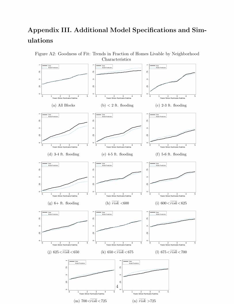
Appendix III. Additional Model Specifications and Sim-

ulations

Figure A2: Goodness of Fit: Trends in Fraction of Homes Livable by NeighborhoodCharacteristics

0.2

5.5

.75

1

0 1 2 3 4 5Years Since Hurricane Katrina

DataModel Prediction

(a) All Blocks

0.2

5.5

.75

10 1 2 3 4 5

Years Since Hurricane Katrina


(b) < 2 ft. flooding

0.2

5.5

.75

1



(c) 2-3 ft. flooding

0.2

5.5

.75

1



(d) 3-4 ft. flooding

0.2

5.5

.75

1



(e) 4-5 ft. flooding

0.2

5.5

.75

10 1 2 3 4 5

Years Since Hurricane Katrina


(f) 5-6 ft. flooding

0.2

5.5

.75

1



(g) 6+ ft. flooding

0.2

5.5

.75

1



(h) risk <600

0.2

5.5

.75

1



(i) 600<risk<625

0.2

5.5

.75

1



(j) 625<risk<650

0.2

5.5

.75

1



(k) 650<risk<675

0.2

5.5

.75

1



(l) 675<risk<700

0.2

5.5

.75

1



(m) 700<risk<725

0.2

5.5

.75

1



(n) risk >725

4

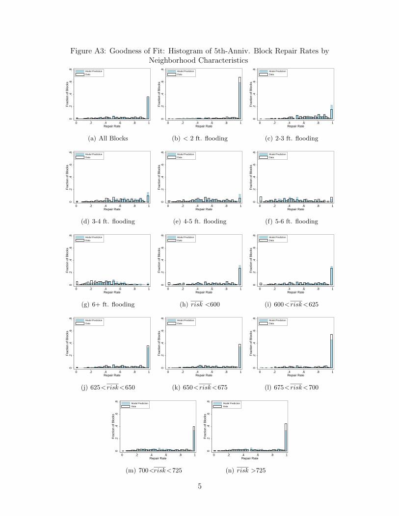
Figure A3: Goodness of Fit: Histogram of 5th-Anniv. Block Repair Rates byNeighborhood Characteristics

0.2

.4.6

.8F

ract

ion

of B

lock

s

0 .2 .4 .6 .8 1Repair Rate

Model PredictionData

(a) All Blocks

0.2

.4.6

.8F

ract

ion

of B

lock

s

0 .2 .4 .6 .8 1Repair Rate


(b) < 2 ft. flooding

0.2

.4.6

.8F

ract

ion

of B

lock

s

0 .2 .4 .6 .8 1Repair Rate


(c) 2-3 ft. flooding

0.2

.4.6

.8F

ract

ion

of B

lock

s

0 .2 .4 .6 .8 1Repair Rate


(d) 3-4 ft. flooding

0.2

.4.6

.8F

ract

ion

of B

lock

s

0 .2 .4 .6 .8 1Repair Rate


(e) 4-5 ft. flooding

0.2

.4.6

.8F

ract

ion

of B

lock

s

0 .2 .4 .6 .8 1Repair Rate


(f) 5-6 ft. flooding

0.2

.4.6

.8F

ract

ion

of B

lock

s

0 .2 .4 .6 .8 1Repair Rate


(g) 6+ ft. flooding

0.2

.4.6

.8F

ract

ion

of B

lock

s

0 .2 .4 .6 .8 1Repair Rate


(h) risk <600

0.2

.4.6

.8F

ract

ion

of B

lock

s

0 .2 .4 .6 .8 1Repair Rate


(i) 600<risk<625

0.2

.4.6

.8F

ract

ion

of B

lock

s

0 .2 .4 .6 .8 1Repair Rate


(j) 625<risk<650

0.2

.4.6

.8F

ract

ion

of B

lock

s

0 .2 .4 .6 .8 1Repair Rate


(k) 650<risk<675

0.2

.4.6

.8F

ract

ion

of B

lock

s

0 .2 .4 .6 .8 1Repair Rate


(l) 675<risk<700

0.2

.4.6

.8F

ract

ion

of B

lock

s

0 .2 .4 .6 .8 1Repair Rate


(m) 700<risk<725

0.2

.4.6

.8F

ract

ion

of B

lock

s

0 .2 .4 .6 .8 1Repair Rate


(n) risk >725

5

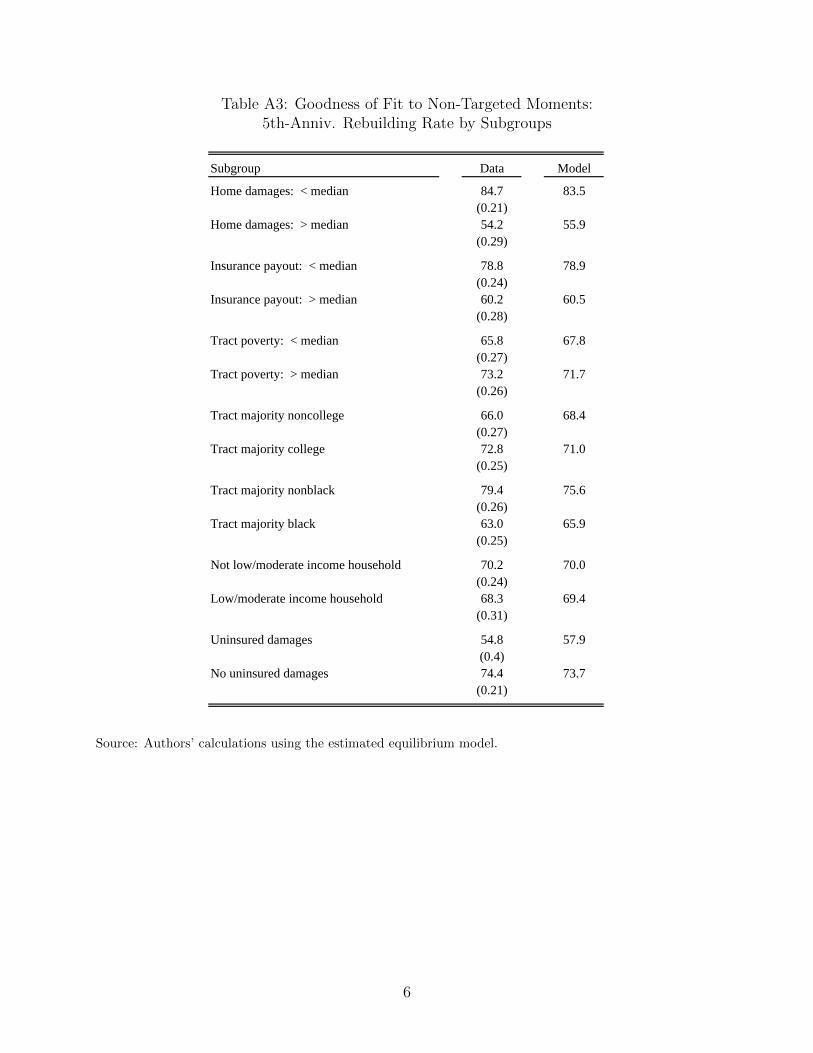
Table A3: Goodness of Fit to Non-Targeted Moments:5th-Anniv. Rebuilding Rate by Subgroups

Subgroup Data Model

Home damages: < median 84.7 83.5(0.21)

Home damages: > median 54.2 55.9(0.29)

Insurance payout: < median 78.8 78.9(0.24)

Insurance payout: > median 60.2 60.5(0.28)

Tract poverty: < median 65.8 67.8(0.27)

Tract poverty: > median 73.2 71.7(0.26)

Tract majority noncollege 66.0 68.4(0.27)

Tract majority college 72.8 71.0(0.25)

Tract majority nonblack 79.4 75.6(0.26)

Tract majority black 63.0 65.9(0.25)

Not low/moderate income household 70.2 70.0(0.24)

Low/moderate income household 68.3 69.4(0.31)

Uninsured damages 54.8 57.9(0.4)

No uninsured damages 74.4 73.7(0.21)

Source: Authors’ calculations using the estimated equilibrium model.

6

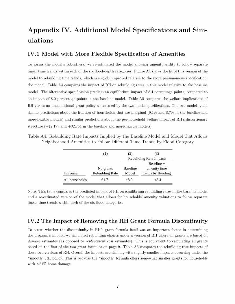
Appendix IV. Additional Model Specifications and Sim-

ulations

IV.1 Model with More Flexible Specification of Amenities

To assess the model’s robustness, we re-estimated the model allowing amenity utility to follow separate

linear time trends within each of the six flood-depth categories. Figure A4 shows the fit of this version of the

model to rebuilding time trends, which is slightly improved relative to the more parsimonious specification.

the model. Table A4 compares the impact of RH on rebuilding rates in this model relative to the baseline

model. The alternative specification predicts an equilibrium impact of 8.4 percentage points, compared to

an impact of 8.0 percentage points in the baseline model. Table A5 compares the welfare implications of

RH versus an unconditional grant policy as assessed by the two model specifications. The two models yield

similar predictions about the fraction of households that are marginal (9.1% and 8.7% in the baseline and

more-flexible models) and similar predictions about the per-household welfare impact of RH’s distortionary

structure (+$2,177 and +$2,754 in the baseline and more-flexible models).

Table A4: Rebuilding Rate Impacts Implied by the Baseline Model and Model that AllowsNeighborhood Amenities to Follow Different Time Trends by Flood Category

(1) (2) (3) (1) (2) (3) (4)

SubgroupNo grants

Rebuilding RateBaselineModel

Beseline +amenity time

trends by flooding SubgroupBaselineModel


trends by floodingBaselineModel


trends by flooding

All 61.7 +8.0 +8.4 All 9.1 8.7 2,177 2,754Flood depth: Flood depth:

< 2 feet 76.2 +4.5 +4.2 < 2 feet 4.8 4.3 140 7462-3 feet 59.7 +14.1 +15.0 2-3 feet 15.7 15.3 7,726 12,1613-4 feet 59.5 +11.2 +13.1 3-4 feet 13.4 14.7 6,133 11,0944-5 feet 46.2 +12.6 +13.1 4-5 feet 14.8 13.5 2,988 -6,2225-6 feet 35.6 +9.3 +10.0 5-6 feet 11.0 10.3 -475 3,139>6 feet 42.4 +8.0 +7.8 >6 feet 9.7 8.3 1,656 1,338

(1) (2) (3) (1) (2) (3) (4)

SubgroupNo grants







trends by flooding


< 2 feet 76.2 +4.5 +4.2 < 2 feet 4.8 4.3 140 7462-4 feet 59.6 +12.7 +14.1 2-4 feet 14.6 15.0 6,954 11,644>4 feet 42.3 +9.8 +10.0 >4 feet 11.6 10.4 1,662 -768

(1) (2) (3) (1) (2) (3) (4)

UniverseNo grants



trends by flooding UniverseBaselineModel




trends by flooding

All households 61.7 +8.0 +8.4 All households 9.1 8.7 2,177 2,754

Rebuilding Rate Impacts % Marginal Welfare Impacts ($ per capita)


Rebuilding Rate Impacts Welfare Impacts ($ per capita)% Marginal

Note: This table compares the predicted impact of RH on equilibrium rebuilding rates in the baseline model

and a re-estimated version of the model that allows for households’ amenity valuations to follow separate

linear time trends within each of the six flood categories.

IV.2 The Impact of Removing the RH Grant Formula Discontinuity

To assess whether the discontinuity in RH’s grant formula itself was an important factor in determining

the program’s impact, we simulated rebuilding choices under a version of RH where all grants are based on

damage estimates (as opposed to replacement cost estimates). This is equivalent to calculating all grants

based on the first of the two grant formulas on page 9. Table A6 compares the rebuilding rate impacts of

these two versions of RH. Overall the impacts are similar, with slightly smaller impacts occurring under the

“smooth” RH policy. This is because the “smooth” formula offers somewhat smaller grants for households

with >51% home damage.

7

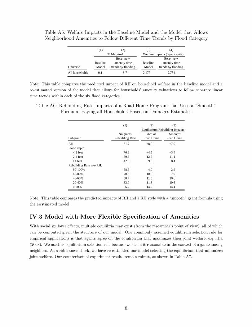
Table A5: Welfare Impacts in the Baseline Model and the Model that AllowsNeighborhood Amenities to Follow Different Time Trends by Flood Category

(1) (2) (3) (1) (2) (3) (4)

SubgroupNo grants







trends by flooding


< 2 feet 76.2 +4.5 +4.2 < 2 feet 4.8 4.3 140 7462-3 feet 59.7 +14.1 +15.0 2-3 feet 15.7 15.3 7,726 12,1613-4 feet 59.5 +11.2 +13.1 3-4 feet 13.4 14.7 6,133 11,0944-5 feet 46.2 +12.6 +13.1 4-5 feet 14.8 13.5 2,988 -6,2225-6 feet 35.6 +9.3 +10.0 5-6 feet 11.0 10.3 -475 3,139>6 feet 42.4 +8.0 +7.8 >6 feet 9.7 8.3 1,656 1,338

(1) (2) (3) (1) (2) (3) (4)

SubgroupNo grants







trends by flooding


< 2 feet 76.2 +4.5 +4.2 < 2 feet 4.8 4.3 140 7462-4 feet 59.6 +12.7 +14.1 2-4 feet 14.6 15.0 6,954 11,644>4 feet 42.3 +9.8 +10.0 >4 feet 11.6 10.4 1,662 -768

(1) (2) (3) (1) (2) (3) (4)

UniverseNo grants



trends by flooding UniverseBaselineModel




trends by flooding

All households 61.7 +8.0 +8.4 All households 9.1 8.7 2,177 2,754



Rebuilding Rate Impacts Welfare Impacts ($ per capita)% Marginal

Note: This table compares the predicted impact of RH on household welfare in the baseline model and a

re-estimated version of the model that allows for households’ amenity valuations to follow separate linear

time trends within each of the six flood categories.

Table A6: Rebuilding Rate Impacts of a Road Home Program that Uses a “Smooth”Formula, Paying all Households Based on Damages Estimates

(1) (2) (3)

SubgroupNo grants

Rebuilding RateActual

Road Home"Smooth"

Road Home

All 61.7 +8.0 +7.0Flood depth:

< 2 feet 76.2 +4.5 +3.92-3 feet 59.7 14.1 11.93-4 feet 59.5 11.2 10.34-5 feet 46.2 12.6 11.45-6 feet 35.6 9.3 7.3>6 feet 42.4 8.0 6.9

Rebuilding Rate w/o RH:90-100% 99.3 0.2 -0.280-90% 85.1 5.3 3.470-80% 75.6 8.8 6.360-70% 66.0 11.0 9.250-60% 55.1 11.2 10.240-50% 45.4 11.8 11.030-40% 36.7 11.7 10.420-30% 26.2 11.9 11.010-20% 16.6 14.7 13.40-10% 4.7 14.9 14.5

(1) (2) (3)

SubgroupNo grants

Rebuilding RateActual

Road Home"Smooth"

Road Home

All 61.7 +8.0 +7.0Flood depth:

< 2 feet 76.2 +4.5 +3.92-4 feet 59.6 12.7 11.1>4 feet 42.3 9.8 8.4

Rebuilding Rate w/o RH:80-100% 88.8 4.0 2.560-80% 70.3 10.0 7.940-60% 50.4 11.5 10.620-40% 33.0 11.8 10.60-20% 6.2 14.9 14.4

Equilibrium Rebuilding Impacts

Equilibrium Rebuilding Impacts

Note: This table compares the predicted impacts of RH and a RH style with a “smooth” grant formula using

the ewstimated model.

IV.3 Model with More Flexible Specification of Amenities

With social spillover effects, multiple equilibria may exist (from the researcher’s point of view), all of which

can be computed given the structure of our model. One commonly assumed equilibrium selection rule for

empirical applications is that agents agree on the equilibrium that maximizes their joint welfare, e.g., Jia

(2008). We use this equilibrium selection rule because we deem it reasonable in the context of a game among

neighbors. As a robustness check, we have re-estimated our model selecting the equilibrium that minimizes

joint welfare. Our counterfactual experiment results remain robust, as shown in Table A7.

8

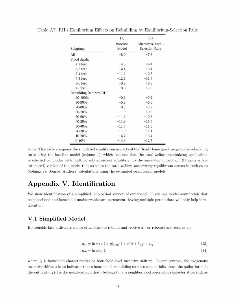
Table A7: RH’s Equilibrium Effects on Rebuilding by Equilibrium-Selection Rule

(1) (2)

Subgroup

Baseline

Model

Alternative Eqm.-

Selection Rule

All +8.0 +7.6

Flood depth:

< 2 feet +4.5 +4.4

2-3 feet +14.1 +13.1

3-4 feet +11.2 +10.5

4-5 feet +12.6 +11.4

5-6 feet +9.3 +8.8

>6 feet +8.0 +7.6

Rebuilding Rate w/o RH:

90-100% +0.2 +0.2

80-90% +5.3 +5.0

70-80% +8.8 +7.7

60-70% +11.0 +9.9

50-60% +11.2 +10.3

40-50% +11.8 +11.4

30-40% +11.7 +11.5

20-30% +11.9 +11.1

10-20% +14.7 +13.4

0-10% +14.9 +12.7

Note: This table compares the simulated equilibrium impacts of the Road Home grant program on rebuilding

rates using the baseline model (column 1), which assumes that the total-welfare-maximizing equilibrium

is selected on blocks with multiple self-consistent equilibria, to the simulated impact of RH using a (re-

estimated) version of the model that assumes the total-welfare-minimizing equilibrium occurs in such cases

(column 2). Source: Authors’ calculations using the estimated equilibrium models.

Appendix V. Identification

We show identification of a simplified, one-period version of our model. Given our model assumption that

neighborhood and household unobservables are permanent, having multiple-period data will only help iden-

tification.

V.1 Simplified Model

Households face a discrete choice of whether to rebuild and receive ui1 or relocate and receive ui0:

ui1 = ln c1(zi) + g(µj(i)) + x′jβ + bj(i) + εij (13)

ui0 = ln c0(zi), (14)

where zi is household characteristics or household-level incentive shifters. In our context, the exogenous

incentive shifter z is an indicator that a household’s rebuilding cost assessment falls above the policy formula

discontinuity. j (i) is the neighborhood that i belongs to, x is neighborhood observable characteristics, such as

9

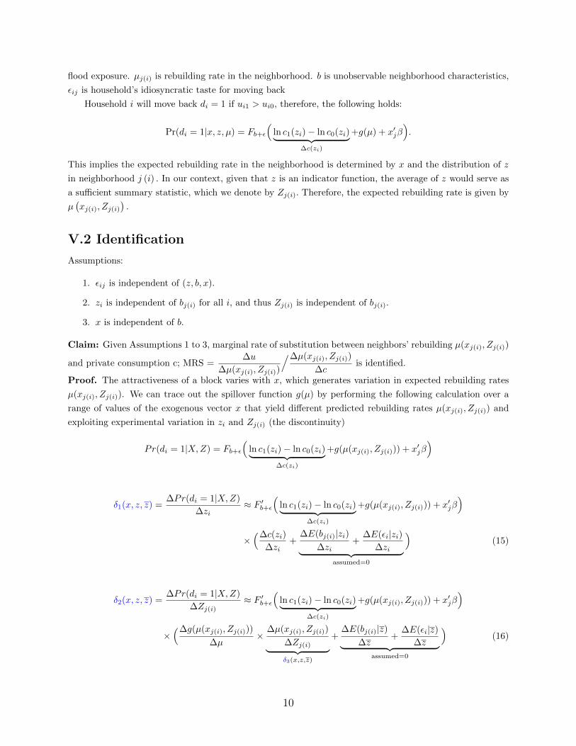
flood exposure. µj(i) is rebuilding rate in the neighborhood. b is unobservable neighborhood characteristics,

εij is household’s idiosyncratic taste for moving back

Household i will move back di = 1 if ui1 > ui0, therefore, the following holds:

Pr(di = 1|x, z, µ) = Fb+ε

(ln c1(zi)− ln c0(zi)︸︷︷︸

∆c(zi)

+g(µ) + x′jβ).

This implies the expected rebuilding rate in the neighborhood is determined by x and the distribution of z

in neighborhood j (i) . In our context, given that z is an indicator function, the average of z would serve as

a sufficient summary statistic, which we denote by Zj(i). Therefore, the expected rebuilding rate is given by

µ(xj(i), Zj(i)

).

V.2 Identification

Assumptions:

1. εij is independent of (z, b, x).

2. zi is independent of bj(i) for all i, and thus Zj(i) is independent of bj(i).

3. x is independent of b.

Claim: Given Assumptions 1 to 3, marginal rate of substitution between neighbors’ rebuilding µ(xj(i), Zj(i))

and private consumption c; MRS =∆u

∆µ(xj(i), Zj(i))

/∆µ(xj(i), Zj(i))

∆cis identified.

Proof. The attractiveness of a block varies with x, which generates variation in expected rebuilding rates

µ(xj(i), Zj(i)). We can trace out the spillover function g(µ) by performing the following calculation over a

range of values of the exogenous vector x that yield different predicted rebuilding rates µ(xj(i), Zj(i)) and

exploiting experimental variation in zi and Zj(i) (the discontinuity)

Pr(di = 1|X,Z) = Fb+ε


∆c(zi)

+g(µ(xj(i), Zj(i))) + x′jβ)

δ1(x, z, z) =∆Pr(di = 1|X,Z)

∆zi≈ F ′b+ε


∆c(zi)


×(∆c(zi)

∆zi+

∆E(bj(i)|zi)∆zi

+∆E(εi|zi)

∆zi︸︷︷︸assumed=0

)(15)

δ2(x, z, z) =∆Pr(di = 1|X,Z)

∆Zj(i)≈ F ′b+ε


∆c(zi)


×(∆g(µ(xj(i), Zj(i)))

∆µ×

∆µ(xj(i), Zj(i))

∆Zj(i)︸︷︷︸δ3(x,z,z)

+∆E(bj(i)|z)

∆z+

∆E(εi|z)∆z︸︷︷︸

assumed=0

)(16)

10

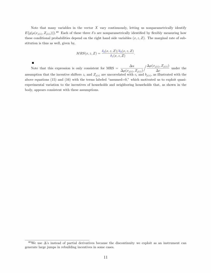
Note that many variables in the vector X vary continuously, letting us nonparametrically identify

E(g(µ(xj(i), Zj(i)))

).40 Each of these three δ’s are nonparametrically identified by flexibly measuring how

these conditional probabilities depend on the right hand side variables (x, z, Z). The marginal rate of sub-

stitution is thus as well, given by,

MRS(x, z, Z) =δ2(x, z, Z)/δ3(x, z, Z)

δ1(x, z, Z).

Note that this expression is only consistent for MRS =∆u

∆µ(xj(i), Zj(i))

/∆µ(xj(i), Zj(i))

∆cunder the

assumption that the incentive shifters zi and Zj(i) are uncorrelated with εi and bj(i), as illustrated with the

above equations (15) and (16) with the terms labeled “assumed=0,” which motivated us to exploit quasi-

experimental variation to the incentives of households and neighboring households that, as shown in the

body, appears consistent with these assumptions.

40We use ∆’s instead of partial derivatives because the discontinuity we exploit as an instrument cangenerate large jumps in rebuilding incentives in some cases.

11

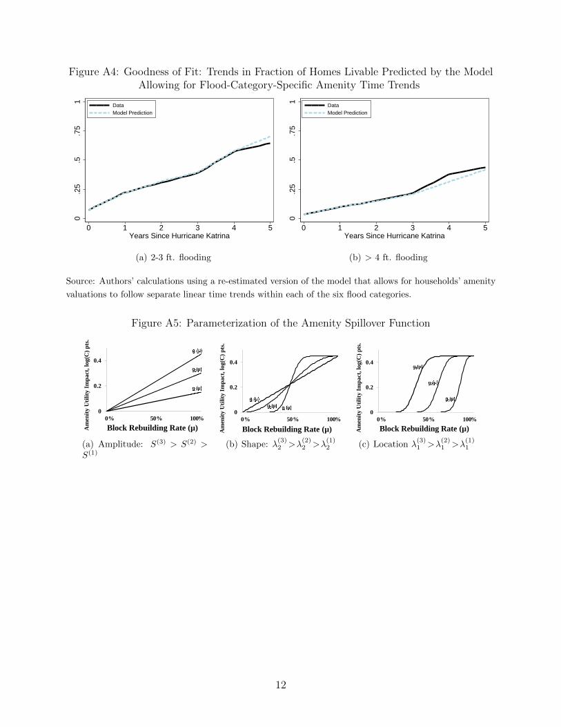
Figure A4: Goodness of Fit: Trends in Fraction of Homes Livable Predicted by the ModelAllowing for Flood-Category-Specific Amenity Time Trends

0.2

5.5

.75

1



(a) 2-3 ft. flooding

0.2

5.5

.75

1



(b) > 4 ft. flooding

Source: Authors’ calculations using a re-estimated version of the model that allows for households’ amenity

valuations to follow separate linear time trends within each of the six flood categories.

Figure A5: Parameterization of the Amenity Spillover Function

0

0.2

0.4

0% 50% 100%

Block Rebuilding Rate (µ)Am

enit

y U

tili

ty I

mp

act,

log(

C)

pts

.

0

0.2

0.4

0% 50% 100%


enit

y U

tili

ty I

mp

act,

log(

C)

pts

.

0

0.2

0.4

0% 50% 100%


enit

y U

tili

ty I

mp

act,

log(

C)

pts

.

(a) Amplitude: S(3) > S(2) >S(1)

0

%

0.1

0.11

0.12

0.13

0.14

0.15

0.16

0.17

0.18

0.19

0.2

0.21

0.22

0.23

0.24

0.25

0.26

0.27

0.28

0.29

0.3

0.31

0.32

0.33

0.34

0.35

0.36

0.37

0.38

0.39

0.4

0.41

5

0

0

0.2

0.4

0% 50% 100%

Block Rebuilding Rate (µ) Am

enit

y U

tili

ty I

mp

act

, lo

g(C

) p

ts.

0

0.2

0.4

0% 50% 100%


enit

y U

tili

ty I

mp

act

, lo

g(C

) p

ts.

0

0.2

0.4

0% 50% 100%


enit

y U

tili

ty I

mp

act

, lo

g(C

) p

ts.

(b) Shape: λ(3)2 >λ

(2)2 >λ

(1)2

0

%

0.1

0.11

0.12

0.13

0.14

0.15

0.16

0.17

0.18

0.19

0.2

0.21

0.22

0.23

0.24

0.25

0.26

0.27

0.28

0.29

0.3

0.31

0.32

0.33

0.34

0.35

0.36

0.37

0.38

0.39

0.4

0.41

5

0

0

0.2

0.4

0% 50% 100%


enit

y U

tili

ty I

mp

act

, lo

g(C

) p

ts.

0

0.2

0.4

0% 50% 100%


enit

y U

tili

ty I

mp

act

, lo

g(C

) p

ts.

0

0.2

0.4

0% 50% 100%


enit

y U

tili

ty I

mp

act

, lo

g(C

) p

ts.

(c) Location λ(3)1 >λ

(2)1 >λ

(1)1

12

Estimation of an Equilibrium Model with Externalities ...cfu/Fu_Gregory.pdf · Estimation of an...

Documents

Transcript of Estimation of an Equilibrium Model with Externalities ...cfu/Fu_Gregory.pdf · Estimation of an...