Estimation in the continuous time mover-stayer modelwith an application to bond ratings migration *

Halina Frydman**Stern School of Business, New York University

Ashay Kadam***University of Michigan Business School

December 19th, 2002

*The authors are very grateful to Roger Stein, Managing Director of Quantitative Risk

Analytics at Moody’s Risk Management Services for providing data and for useful discus-

sions. We thank Petra Miskov for her very skillful work on organizing and analyzing the

data. Halina Frydman’s research on this paper was supported by the summer research

grant from the Stern School of Business at New York University.

**Information, Operations and Management Sciences, email: hfrydman@stern.nyu.edu

***Statistics and Management Science Department, email: ashay@umich.edu

Abstract

The usual tool for modeling bond ratings migration is a discrete, time-homogeneuous Markov chain. Such model assumes that all bonds are ho-mogeneous with respect to their movement behavior among rating categoriesand that the movement behavior does not change over time. However, amongrecognized sources of heterogeneity in ratings migration is age of a bond (timeelapsed since issuance). It has been observed that young bonds have a lowerpropensity to change ratings, and thus to default, than more seasoned bonds.The aim of this paper is to introduce a continuous, time-nonhomogeneuous

model for bond ratings migration, which also incorporates a simple form ofpopulation heterogeneity. The specific form of heterogeneity postulated bythe proposed model appears to be suitable for modeling the effect of age of abond on its propensity to change ratings. This model, called a mover-stayermodel, is an extension of a time-nonhomogeneuous Markov chain.This paper derives the maximum likelihood estimators for the parameters

of a continuous time mover-stayer model based on a sample of independentcontinuously monitored histories of the process, and develops the likelihoodratio test for discriminating between the Markov chain and the mover-stayermodel. The methods are illustrated using a sample of rating histories ofyoung corporate issuers. For this sample, the likelihood ratio test rejectsa Markov chain in favor of a mover-stayer model. For young bonds withlowest rating the default probabilities predicted by the mover-stayer modelare substantially lower than those predicted by the Markov chain.

Keywords: Ratings migration, mover-stayer model, Markov chain, esti-mation

JEL Classification: C13, G33

1 Introduction

The usual tool for modeling bond ratings migration is a time-homogenous,discrete Markov chain. Such modeling assumes that all bond issues are ho-mogeneous with respect to their movement behavior among rating categoriesand also that their behavior does not change over time. However, there aremany sources of heterogeneity in the rating behavior, of which the age of a

2

bond has been recognized as an important one. Evidence presented by Alt-man(1998), Asquith et al, (1989), and Keenan, Soberhardt, and Hamilton(1999) and references therein suggests that propensity of bonds to changerating, and in particular to default, is lower during the early years after is-suance than it is for seasoned bonds. However, this aspect of aging effect hasnot yet been incorporated in any systematic way in modeling of the evolutionof ratings.In this paper we propose a continuous time mover-stayer model to cap-

ture the aging effect described above.1 This model is an extension of a time-nonhomogeneuous, continuous Markov chain. It postulates a simple form ofheterogeneity: a population of bonds is assumed to consist of two subpopu-lations, “movers” and “stayers”. “Movers” evolve according to a continuoustime Markov chain, whereas “stayers” stay in their initial states. The pro-portion of stayers in each rating state is a parameter of the model and can beinterpreted as a measure of immobility for the bonds in a given rating state.If this parameter is zero in each rating, the mover-stayer model reduces toa Markov chain. The mover-stayer model, which allows for a greater degreeof immobility of bonds than a Markov chain, may be a better description ofratings migration for younger bonds. This paper develops a methodology forestimation and testing of this model against the continuous Markov chain.We consider a time-nonhomogeneuous mover-stayer model with time mea-

sured since the issuance of the bond. More precisely the age-nonhomogeneityis modeled by assuming that the parameter of the mover-stayer model is apiece-wise constant function of age with a constant value for each year oflife of the bond. In addition, according to the mover-stayer model, in eachyear of life a bond may exhibit a stayer or a mover type behavior. Thus,the proposed model incorporates both time (age) nonhomogeneity, as well assimple heterogeneity in the movement behavior of bonds that are of similarage.Throughout we consider a continuous time framework, rather than a dis-

crete one, because rating agencies (Moody’s, Standard and Poor’s) monitor

1The discrete time mover-stayer model which was introduced by Blumen, Kogan andMcCarthy (1955) has been since employed in many areas (e.g. Colombo and Morrison(1989), Sampson (1990), Chaterjee and Ramaswamy (1996), and Chen et al (1997)). Fry-dman, Kallberg and Kao (1985) applied the estimation methods for the discrete timemover-stayer model developed in Frydman (1984) to the analysis of credit behavior. Sub-sequently, Altman and Kao (1991) used this methodology in their study of ratings migra-tion.

3

changes in bond ratings on daily basis which gives rise to very detailed data.For a given bond issue the complete history of its rating changes is available,which includes the exact dates of rating changes, the types of the changes thatoccur, and the lengths of stay in different rating states. Modeling such datausing only information obtained at discrete time points would necessarily en-tail a loss of information. In addition, a continuous time framework affordsa possibility of making predictions of quantities of interest, such as of futurerating state probabilities, at any relevant time horizon, whereas the predic-tions with a discrete version of the model can be made only at times that aremultiples of the sampling interval. Until recently a discrete time frameworkhas been employed almost exclusively to model rating migrations. The firststatistical analysis of ratings migration with a continuous time Markov chainhas been in Lando and Skodeberg (2000) to which the reader is referred for amore extensive discussion of the advantages of a continuous time frameworkand related recent references.To implement the continuous time mover-stayer model, we derive the

maximum likelihood (ml) estimators of its parameters based on a sample ofindependent continuously observed realizations from this process. The mlestimation in the continuous time mover-stayer model from continuously ob-served realizations has not been considered before.2 ,3 Based on the derivedml estimators we formulate the likelihood ratio test for discriminating be-tween the Markov chain and the mover-stayer models. The main tool forobtaining the ml estimators is the EM algorithm (Dempster, Laird, and Ru-bin (1977)). However, we show that when realizations are observed over thesame fixed time horizon, the ml estimators can be easily obtained by directmaximization of the likelihood function.We illustrate our methods using the rating histories of the sample of 856

corporate bond issuers that were observed in the period from January, 1985to December, 1995. On the basis of this sample, we estimate the continu-ous age-nonhomogeneous mover-stayer model and Markov chain. The age-nonhomogeneity is modeled by assuming that the parameter of the process

2Maximum likelihood estimation in the discrete time mover-stayer model was discussedin Frydman (1984), Fuchs and Greenhouse (1988), and Swensen (1996). Bayesian estima-tion in the continuous time mover-stayer model from panel data was considered in Fougereand Kamionka (2002).

3Maximum likelihood estimation in the mixtures of continuous time Markov chains thatgeneralize the mover-stayer model is considered in Frydman (2002). Another generalizationof the discrete time mover-stayer model is in Cook et al. (2001).

4

is a step function which is constant within each one-year age interval, that is,the models are estimated separately for bonds in their first year of life, thesecond year of life, etc, yielding age specific one-year transition probabilitymatrices.4 Because of data limitation we estimate the two models only up tothe fifth year of life of the bond.We briefly summarize our empirical results reported in Section 4. The

likelihood ratio test rejects the Markov chain in favor of the mover-stayermodel in each of the one-year age intervals. The overall expected proportionof stayers estimated by the mover-stayer model is large for very young bondsand then decreases as bonds become more seasoned. This is consistent withthe aging effect. The interesting aspect of our results is the large estimatedproportion of stayers in the C (combined Caa, Ca and C) rating for youngbonds. This has a substantial implication for the estimation of the probabil-ity of default from rating C: for young bonds one-year probabilities of defaultfrom rating C estimated by the mover-stayer model are substantially smallerthan those estimated by a Markov chain. The difference in the default prob-abilities resulting from the two models is largest for very young bonds andthen decreases with age. For both models the probability of default is largestin the fifth year and much smaller for younger bonds. We do note that ourresults are based on a small sample of bonds and thus we treat the empiricalanalysis solely as an illustration of the methodology. An application of themethodology developed here to a much larger sample is required to evaluatethe usefulness of the continuous-time mover stayer model in modeling theaging effect.This paper is organized as follows. In Section 2 we define the mover-

stayer model in continuous time and its time nonhomogeneuous version whichwe use to model aging effect. Section 3 develops the ml estimation in themover-stayer model from continuous observations. In Section 4 we reportand discuss the results of the estimation of the mover-stayer model and theMarkov chain for ratings migration of young bond issuers.

4We note that the one-year transition matrix for a portfolio containing bonds of differentages can then be estimated by the weighted average of the age specific one-year transitionmatrices with the weights representing the proportions of bond issuers of different ages.

5

2 The mover-stayer model

To define a mover-stayer model in continuous time we first consider a Markovchain in continuous time with state space W = (1, 2, ..., w). The states cor-respond to different rating categories. Such chain is characterized by thegenerator matrix Q, which is the matrix with the following structure

qii ≤ 0, qij ≥ 0,Xj 6=i

qij = −qii ≡ qi, i ∈W.

In the context of our application to ratings migration the entries inQ havethe following probabilistic interpretation: each time a bond enters rating iit stays in it for the time that is exponentially distributed with parameter(−qii) . When it exits from rating i, it makes a transition to rating j, j 6= iwith probability qij/ (−qii) . In particular,

1

−qii = expected length of time for an issuer in

rating i to remain in that rating.

Matrix Q is called a generator, because it generates M(t), the matrix oftransition probabilities mij(t) of a continuous time Markov chain. M(t) isobtained, for every time t, by exponentiation of tQ, that is,

M(t) = exp(tQ), t ≥ 0.

For the definition of the matrix exponential and an exposition of Markovchains in continuous time see, for example, Norris (1997).A continuous time mover-stayer model on state space W ={1, 2, .., w} is

a mixture of two independent Markov chains, one which evolves according tosome infinitesimal generator Q, and the other whose transition probabilitymatrix is an identity matrix I. The transition probability matrix, P (t), of acontinuous time mover-stayer model on state space W is then defined as

P (t) = SI + (I − S) exp(tQ), t ≥ 0, (1)

where S =diag(s1, s2, ..., sw), with

si = proportion of stayers in state i, i ∈W.

6

The Markov chain defined above is time homogeneous because its generatoris constant in time. Similarly the mover-stayer model defined above is timehomogeneous because it involves a time homogeneous Markov chain, andproportions of stayers that do not change over time.A time-nonhomogeneous Markov chain has a generator Q(t) which is a

function of time. A simple, but for our purpose very useful, time-nonhomogeneousMarkov chain can be defined by assuming that its generator, Q(t), is a piece-wise constant function of time on some time interval (0, T ) that correspondsto the time of the study. The particular specification of Q(t) of interest tous is

Q(t) = Q(1), 0 ≤ t ≤ 1, (2)

= Q(2), 1 < t ≤ 2,...

= Q(m),m− 1 < t ≤ m = T

where 1, 2, ...,m−1 are the times where regime changes occur and Q(k) is thegenerator in the k0th time subinterval, 1 ≤ k ≤ m. With the view towardsour application, we assume that time is measured in years since the issuanceof the bond so that the generator in (2) depends on the age of the bond issuerand the one-year transition probability matrix for bonds age (k− 1) is givenby

M(k − 1, k) = exp(Q(k)), 1 ≤ k ≤ m− 1.We define the time-nonhomogeneous mover-stayer model by assuming

that a generator of a Markov chain which describes the evolution of moversis as in (2). Furthermore, we assume that a bond in state i at the beginningof the k’th one-year age interval, (k − 1, k), has probability si(k) of beinga stayer in that interval independently of its behavior in the preceding ageintervals. Thus, the k’th age interval has its own vector of proportions ofstayers, denoted by s(k) = (si(k), 1 ≤ i ≤ w). The k’th one-year age intervaltransition probability matrix is then given by

P (k − 1, k) = S(k) + (I − S(k)) exp(Q(k)), 1 ≤ k ≤ m− 1,

where S(k) =diag(s1(k), s2(k), ..., sw(k)). The transition matricesM(k−1, k)and P (k− 1, k), 1 ≤ k ≤ m− 1, are age specific one-year transition matricesfor the Markov chain and mover-stayer model respectively.

7

We note that for both models we can easily compute the transition prob-ability matrix between arbitrary times s, t such that 0 ≤ s ≤ t ≤ m. Forexample, setting s = 0.5 and t = 2.5, the transition probability matrixM(s, t) of a Markov chain with generator in (2) is

M(0.5, 2.5) = exp(0.5Q(1)) exp(Q(2)) exp(0.5Q(3)), (3)

and the transition matrix P (s, t) of a mover-stayer model is

P (0.5, 2.5) = [S(1) + (I − S(1)) exp(0.5Q(1))]

× [S(2) + (I − S(2)) exp(Q(2))] (4)

× [S(3) + (I − S(3)) exp(0.5Q(3))] .

The expression in (3) follows by Markov property and the expression in (4)by the definition of the mover-stayer model which implies that the model hasMarkov property at discrete time (age) points 0, 1, ...,m, but behaves as themover-stayer model within each age interval.For both a Markov chain and a mover-stayer model the estimation of

their parameters can be done separately in each one-year age interval. Byassumption in each such time interval both models are time homogeneous.Thus, to estimate the generator in (2) for a Markov chain, we use the mlestimate of Q(k) using the data on bonds with age (time since issuance) inthe interval (k − 1, k). This is a well known ml estimator of the generator ofa time homogeneous Markov chain and is presented in Section 3.1. Similarlywe estimate Q(k) and S(k) in the mover-stayer model based on bonds withage in the interval (k − 1, k). The ml estimators of these parameters, thatis, of the parameters of a time homogeneous mover-stayer model are derivedbelow.

3 Maximum Likelihood Estimation

Let X = (Xt, t ≥ 0), be a mover-stayer model with transition probabilityfunction defined in (1). Assume that we observe n independent realizationsof X and that the k’th realization, Xk, is observed continuously on sometime interval [0, T k] with T k ≤ T, where T is the time horizon of the study.Thus, Xk = (Xt, 0 ≤ t ≤ T k) and individual realizations may be observedover time intervals of different lengths. This may be the case when rightcensoring is present or when the mixture process has an absorbing state.

8

The right censoring is assumed to be independent. Let A be the set of allrealizations that stayed continuously in an initial state, and B be the set ofall realizations with at least one transition. We note that A may containmovers as well as stayers.Let LQ

k be the likelihood of observingXk when it is generated by a Markov

chain with an intensity matrix Q. Then conditional on knowing an initialstate (see e.g., Albert (1962)),

LQk =

Yi 6=j(qij)

nkijYi

exp(−qiτki ),

where

nkij = the number of times Xk makes an i→ j transition, i 6= j,

τki = the total time Xk spends in state i.

Thus, the likelihood of Xk ∈ B under the mover-stayer model, conditionalon knowing an initial state is

wYi=1

(1− si)Iki LQ

k ,

and the similar likelihood for Xk ∈ A is

Lk =wYi=1

(si)Iki +

wYi=1

(1− si)Iki LQ

k ,

where

Ikr = 1 if Xk0 = r

= 0, otherwise.

It is seen that the likelihood function of n independent realizations, L ≡Qnk=1 Lk, is difficult to maximize directly. Instead we develop the EM algo-

rithm for obtaining the mles of Q and s. To implement this algorithm werequire Qc and sc, the mles of the parameters based on complete information.The derivation of Qc and sc, is straightforward, but we include it below forcompleteness and also to introduce the notation needed for the formulationof the EM algorithm. Let

Y k = 1, if the k’th realization is generated by a stayer,

0, otherwise.

9

Obviously, for any realization with nonzero number of transitions, Y k = 0,and for any realization with zero transitions, Y k is not observed. Assumingthat all Y ks are observed, Lc

k, the likelihood function of the kth realization

of the mover-stayer model is simply

Lck =

wYr=1

(sr)Ikr Yk (1− sr)

Ikr (1−Yk)ÃY

i6=j(qij)

nkijYi

exp(−qiτki )!1−Yk

,

or

logLck =

wXr=1

Ikr log(1− sr) + Yk

wXr=1

Ikr log [sr/(1− sr)]

+(1− Yk)Xi6=j

nkij log(qij)− (1− Yk)Xi

¡qiτ

ki

¢,

which for all realizations becomes

logLc =wXr=1

mr log(1− sr) +wXr=1

mSr log [sr/(1− sr)]

+Xi6=j

nij log(qij)−Xi

qiτ i +Xi

qiτSi ,

where

mr =wXr=1

Ikr = total number of individuals that begin in state r,

mSr =

nXk=1

Ikr Yk = number of stayers in state r

nij =nX

k=1

nkij = total number of i→ j transitions in the sample,

ni =wXj 6=i

nij = total number of transitions out of state i

τ i =nX

k=1

τki = total time in state i for all individuals in the sample,

τSi =nX

k=1

Ykτki = the total time in state i for stayers, τ

Mi = τ i − τSi

10

Solving the score equation ∂ logLc/∂si = 0, gives the natural estimatorbsci = mSi /mi. Now setting ∂ logLc/∂qij = 0, we obtain

qcij =nij

τ i − τSi=

nijτMi

, (5)

and fromPw

j 6=i qij = qi,

qci =wXj 6=i

nijτMi

=niτMi

, (6)

From (5) and (6) we also get

qcij =nijni

qi. (7)

3.1 The EM algorithm

Based on the mles assuming complete information we develop the EM al-gorithm for the estimation of the parameters (si, qi, i ∈ W ). We note thatbecause of (7) we don’t have to update the value of qij, j 6= i, at each iter-ation of the algorithm. After the algorithm converges to (bsi, qi, i ∈ W ), wecompute qij using (7).

1. InitializeAt the p+ 1st iteration, p ≥ 0, set the values of (si, qi, i ∈W ) to:

spi , qpi , i ∈W.

Define Qp to be the intensity matrix with the entries given by qpij =(nij/ni)q

pi , i 6= j, and qpii = −qpi .

2. Expectation stepFor the k’th history, which starts in state r, 1 ≤ k ≤ n, r ∈W, and doesnot make any transition compute the probability that it is generatedby a stayer:

Ep(Yk) =spr

spr + (1− spr) exp(−qprτkr).

For the k’th history with at least one transition set

Ep(Yk) = 0.

11

Then compute the following expectations

Ep(τSi ) =nX

k=1

τkiEp(Yk),

Ep(τQi ) = τ i − Ep(τSi ),

Ep(mSi ) =

nXk=1

Iki Ep(Yk),

3. Maximization step

Compute the quantities

sp+1i =Ep(mS

i )

mi,

andqp+1i =

ni

Ep(τQi ).

4. Iterate

Go back to Step 2 and iterate until convergence.

3.2 The special case of identical observation horizons

In a special case when all realizations are observed continuously during afixed period of time [0, T ], the estimates of the parameters can be easilyobtained by direct maximization of the likelihood function. In this case wedefine

ar = number of realizations that stay continuously in state r

br = number of realizations with at least one transition that start in state r,

τAi = total time in state i for histories with no transitions,

τBi = total time in state i for histories with at least one transition,

The likelihood function, LA(Q, s), of the realizations in set A is

LA(Q, s) =Yk∈A

(Yr

[sr + (1− sr) exp(−qrT )]Ikr)

(8)

=Yr

[sr + (1− sr) exp(−qrT )]ar ,

12

and the likelihood function, LB(Q, s), of the realizations in B is

LB(Q, s) =Yk∈B

(Yr

(1− sr)Ikr

"Yj 6=i

qnkijij

Yi

exp(−qiτki )#)

(9)

=Yr

(1− sr)brYj 6=i

qnijij

Yi

exp(−qiτBi ),

Thus, the overall loglikelihood function becomes

logL(Q, s) = logLA(Q, s) + logLB(Q, s)

=Xr

ar log sr + (1− sr) exp(−qrT ) (10)

+Xr

br log(1− sr) +Xj 6=i

nij log qij −Xi

qiτBi .

The score equation with respect to sr

∂ logL

∂sr=

ar[1− exp(−qrT )]sr + (1− sr) exp(−qrT ) −

br1− sr

= 0,

gives

sr =ar −mr exp(−qrT )mr −mr exp(−qrT ) . (11)

Substituting (11) into (10), we obtain, up to the terms not depending on theparameters,

logL(Q, s) ∼ −Xr

br log(1− exp(−qrT )) +Xj 6=i

nij log qij −Xi

qiτBi . (12)

From the score equation

∂ logL

∂qij=

biT

1− exp(qiT ) +nijqij− τBi = 0,

we get

qij =nij(exp(qiT )− 1)

Tbi + τBi (exp(qiT )− 1)=

nijTbi(exp(qiT )− 1)−1 + τBi

. (13)

13

Now taking into account thatP

j 6=i qij = qi, gives the following equation forqi

niTbi(exp(qiT )− 1)−1 + τBi

= qi, (14)

which can be rewritten as

(ni − qiτBi )(exp(qiT )− 1) = qiTbi. (15)

It follows from (15), that qi < ni/τBi . The equation (14) can be easily solved

in an iterative fashion for q. At the n’th iteration the left hand side of thisequation is evaluated at q(m)i . This results in the value q(m+1)i . The iterationsare repeated until convergence is achieved. The starting value for qi couldbe taken as any value in the interval (0, ni/τBi ).By (13), the estimates ofthe transition rates qij are given by qij = (nij/ni)qi, and the estimate of si isobtained from (11).

3.3 The likelihood ratio test

We note that the a Markov chain can be obtained from the mover-stayermodel by setting all si equal to zero, that is, a Markov chain is nested inthe mover-stayer model. This allows us to use the likelihood ratio statisticto test a Markov chain model against a mover-stayer model. The hypothesistest is of the form H0 : s = 0 versus H1 : s 6= 0, where the equality s = 0and the inequality should be understood in the vector sense. The likelihoodratio statistic is

Λ = supQ,s=0

L(Q, s)/ supQ,s

L(Q, s) = L(C, 0)/L(Q, s).

Here C is the mle of the intensity matrix Q under H0, that is, when theprocess is assumed to be aMarkov chain, and Q, s are the mles of the intensitymatrix and fractions of stayers, respectively, in the mover-stayer model. Bythe standard result, under H0, the asymptotic distribution of −2 logΛ is χ2with w degrees of freedom.We now compute−2 logΛ.Wewrite the likelihood function for the mover-

stayer model as L(Q, s) = LA(Q, s)LB((Q, s), where, LB((Q, s) is given in(9), and

LA(Q, s) =Yk∈A

(Yr

£sr + (1− sr) exp(−qrτkr)

¤Ikr) ,

14

Note that this is more general than (8), because here we do not assumethat realizations are observed over the same time horizons. The likelihoodfunction of the observations under H0 evaluated at C is

L(C, 0) =Yk

ÃYi6=j(cij)

nkijYi

exp(−ciτki )!,

where cij = (nij/ni) ci, and ci = ni/τ i. In order to simplify the expression for−2 logΛ, we write L(C, 0) = LA(C, 0)LB(C, 0), where

LA(C, 0) =Yk∈A

ÃYi

exp(−ciτki )!= exp

Ã−Xi

ciτAi

!

LB(C, 0) =Yk∈B

nkijYj 6=i

Yi

exp(−ciτki ) =Y

k∈B

"Yj 6=i(nijni

ci)nkijYi

exp(−ciτki )#

Now, evaluating L(Q, s) at Q, s, and noting (7), we obtain

Λ =LA(C, 0)

LA(Q, s)

Yi

½µciqi

¶ni

exp£(qi − ci)τ

Bi

¤¾=

Yi

½µciqi

¶ni

exp(qiτBi − ciτ i)

¾/LA(Q, s)

=Yi

½µciqi

¶ni

exp(qiτBi − ni)

¾/LA(Q, s),

or

−2 logΛ = −2(X

i

ni log

µciqi

¶+Xi

(qiτBi − ni)− logLA(Q, s)

). (16)

For the case of realizations observed over fixed time horizon (0, T ), using (8)and (11), we get

−2 logΛ = −2(X

i

ni log

µciqi

¶+Xi

(qiτBi − ni)−

Xi

ai log(ai/mi)

).

15

4 Application to bond ratings migration

4.1 The Data and the Methods

The data consist of the rating histories of 856 corporate bond issuers in theindustrial sector that were observed for some time in the period from January,1985 to December, 1995. The data was obtained fromMoody’s and thus usesMoody’s rating system. As is customary, and in our case necessary due tothe small sample size, we grouped the original ratings into eight states: Aaa,Aa, A, Baa, Ba, B, C, D and WR where the ratings are ordered from thehighest to the lowest with Aaa being the top ranking, D being the defaultstate and WR denoting the state of rating withdrawal. This resulted in aninitial distribution of 7, 50, 131, 119, 264, 256, 29, 0, 0 bonds in these states,respectively. Thus a majority of the bonds under consideration were issuedwith Ba or B rating.About 30% of issuers entered the sample after 1990, thus providing us

with only with relatively short times under study. Because of this samplelimitation we decided to study aging effect only in the first five years of life ofthe bonds. To study this effect we estimate a time-nonhomogeneuous Markovchain and a mover-stayer model defined in Section 2 on the age interval (0, 5).In both processes time t represents age of the bond issuer. Thus, we assumethat a generator of a Markov chain, Q(t), is a piecewise constant function ofage:

Q(t) = Q(1), 0 ≤ t ≤ 1, (17)

= Q(2), 1 < t ≤ 2,...

= Q(5), 4 < t ≤ 5,

and in case of a mover-stayer model, that the k0th one-year age interval hasits own vector of proportions of stayers, s(k) = (si(k), 1 ≤ i ≤ 8), 1 ≤ k ≤ 5,where i refers to a rating.We now discuss estimation of the age specific transition matrices under

the two models. To obtain these matrices under a Markov model we firstestimate Q(k) for each age interval. The mle C(k) of Q(k), is given by (seefor example, Andersen et al. (1993))

16

cij(k) =nij(k − 1, k)R kk−1 Yi(s)ds

, i 6= j, cii(k) = −Xj 6=i

cij(k) ≡ −ci(k) (18)

where nij(k − 1, k) is the total number of i→ j transitions for all issuers inthe k0th year of their life and Yi(s) is the number of issuers in rating categoryi at time s. Thus,

R kk−1 Yi(s)ds is the total exposure time in rating category

i in the age interval (k − 1, k). We note that the estimators cij(k) use all ofthe available information and do not require that an issuer be present for thewhole observation period.To estimate the age specific transitions matrices under the mover-stayer

model we estimate for each age interval the generator for the movers andthe vector of proportions of stayers using the EM algorithm developed inSection 3.1. After testing that the algorithm converged to the same finalvalues for different initial values we chose the initial values for the algorithmin the following way. For each one-year age interval we chose the observedproportion of bonds that stayed in a rating for that whole interval as aninitial value for the proportion of stayers in this rating. For the k0th ageinterval we chose ci(k), as the initial value for qi, 1 ≤ i ≤ 8, where ci(k) isgiven in (18).

4.2 Estimation results

We summarize here the results of the estimation of the mover-stayer and theMarkov chain models for the five age intervals. As default probabilities playan important role in the pricing of bonds and other related applications infinance, the main focus of the summary will be the comparison of defaultprobabilities estimated by the two models.First, for the purpose of the illustration we report and compare the results

of the estimation of the two models for the age interval (2, 3). The resultsare in Tables 1-6. We note (Table 4) that for this age interval there is a veryhigh proportion of stayers in rating C (81%). As a result the CC entry inthe mover-stayer transition matrix (Table 6) is much larger (0.8594) than thecorresponding one in the Markov chain transition matrix (Table 3) (0.7288).Since there is little movement out of the C rating to other nondefault ratings,this, in turn, results in the smaller default probability from the C rating inthe mover-stayer model (0.0826) as compared to the Markov chain estimate(0.1569). Rating Baa also has a relatively high proportion of stayers (56%)

17

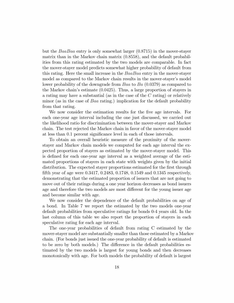
but the BaaBaa entry is only somewhat larger (0.8715) in the mover-stayermatrix than in the Markov chain matrix (0.8558), and the default probabil-ities from this rating estimated by the two models are comparable. In factthe mover-stayer model predicts somewhat higher probability of default fromthis rating. Here the small increase in the BaaBaa entry in the mover-stayermodel as compared to the Markov chain results in the mover-stayer’s modellower probability of the downgrade from Baa to Ba (0.0379) as compared tothe Markov chain’s estimate (0.0425). Thus, a large proportion of stayers ina rating may have a substantial (as in the case of the C rating) or relativelyminor (as in the case of Baa rating.) implication for the default probabilityfrom that rating.We now consider the estimation results for the five age intervals. For

each one-year age interval including the one just discussed, we carried outthe likelihood ratio for discrimination between the mover-stayer and Markovchain. The test rejected the Markov chain in favor of the mover-stayer modelat less than 0.1 percent significance level in each of those intervals.To obtain an overall heuristic measure of the proximity of the mover-

stayer and Markov chain models we computed for each age interval the ex-pected proportion of stayers as estimated by the mover-stayer model. Thisis defined for each one-year age interval as a weighted average of the esti-mated proportions of stayers in each state with weights given by the initialdistribution. The expected stayer proportions estimated for the first throughfifth year of age were 0.3417, 0.2483, 0.1748, 0.1549 and 0.1345 respectively,demonstrating that the estimated proportion of issuers that are not going tomove out of their ratings during a one year horizon decreases as bond issuersage and therefore the two models are most different for the young issuer ageand become similar with age.We now consider the dependence of the default probabilities on age of

a bond. In Table 7 we report the estimated by the two models one-yeardefault probabilities from speculative ratings for bonds 0-4 years old. In thelast column of this table we also report the proportion of stayers in eachspeculative rating for each age interval.The one-year probabilities of default from rating C estimated by the

mover-stayer model are substantially smaller than those estimated by aMarkovchain. (For bonds just issued the one-year probability of default is estimatedto be zero by both models.) The difference in the default probabilities es-timated by the two models is largest for young bonds and then decreasesmonotonically with age. For both models the probability of default is largest

18

in the fifth year and much smaller for younger bonds.The two models estimate similar probabilities of default from rating B for

all considered ages with the mover-stayer proving somewhat larger estimatesfor 1-2 years old bonds. These probabilities increase with age in a monotonicfashion reflecting the aging of the bonds. The estimated proportion of stayersin rating B declines from 15% in the first year of bond issuer’s life to 0 in thefifth year. This explains the virtual equality of probabilities of default fromB estimated by the two models in the fifth year of life of the bonds. Thereis no clear age pattern in the estimated probabilities of default from ratingBa. However, the estimates of default probabilities from this rating in thetwo models are again closer for older bonds.Our empirical results show that for 1-4 years old bonds the mover-stayer

model estimates substantially lower default probabilities from rating C thana Markov chain. These probabilities are particularly different for 1 and 2years old bonds. It also estimates somewhat different default probabilitiesthan a Markov chain from other speculative ratings for 1 and 2 years oldbonds. The empirical discrepancy suggests that a mover-stayer model, asa model subsuming a Markov chain, may provide, in particular for youngerbonds, more accurate estimates of the default probabilities than a mover-stayer model. However, a much larger sample of bonds is needed to furtherassess this possibility.

References

Albert, A. (1962) Estimating the Infinitesimal Generator of a ContinuousTime, Finite State Markov Process, Annals of Mathematical Statistics. 38,727-753.

Altman, E. I. (1998) The Importance and Subtlety of Credit Rating Mi-gration. Journal of Banking and Finance. 22, 1231-1247.

Altman, E. I. and Kao, D. L. (1991) Examining and Modeling CorporateBond Rating Drift. New York University Salomon Center Working PaperSeries s-91-39.

Andersen, P. K., Borgan, O., Gill, R.D., and Keiding, N. (1993) StatisticalModels Based on Counting Processes. New York, Springer-Verlag.

19

Asquith, P., Mullins, D.W., and Wolff, E.D. (1989) Original Issue HighYield Bonds: Aging Analyses of Defaults, Exchanges, and Calls. The Journalof Finance. 44, 923-952.

Blumen, I., Kogan, M., andMcCarthy, P.J. (1955)The Industrial Mobilityof Labor as a Probability Process, Cornell Studies of Industrial and LaborRelations, vol. 6, Ithaca, N.Y., Cornell University Press.

Chatterjee, R. and Ramaswamy, V. (1996), An Extended Mover-StayerModel for Diagnosing the Dynamics of Trial and Repeat for a New Brand.Applied Stochastic Models and Data Analysis, Vol. 12, 165-178.

Chen, H. H., Duffy, S. W. and Tabar, L. (1997) A Mover-Stayer Mixtureof Markov Chain Models for the Assessment of Dedifferentiation and TumorProgression in Breast Cancer. Journal of Applied Statistics 24 (3), 265-278.

Colombo, R. A. and Morrison, D. G. (1989)) A Brand Switching Modelwith Implications for Marketing Strategies. Marketing Science, 8 (Winter),89-99.

Cook, R. J., Kalbfleisch, J. D. and Yi, Y. (2001) A Generalized Mover-Stayer Model for Panel Data.

Dempster, A.P., Laird, N.M. and Rubin, D.B. (1977) Maximum likelihoodfrom incomplete data via the EM algorithm (with discussion).Journal ofRoyal Statistical Society, Series B, 39, 1-38.

Fougère, D. and Kamionka, T., (2002) Bayesian Inference for the Mover-Stayer Model in Continuous Time with an Application to Labour MarketTransition Data., forthcoming in Journal of Applied Econometrics.

Frydman, H., (1984) Maximum Likelihood Estimation in the Mover-Stayer Model., Journal of the American Statistical Association, 79, 632-637.

Frydman, H., Kallberg, J.G., and Kao, D.L. (1985) Testing the adequacyof Markov chains and mover-stayer models as representations of credit be-havior., Operations Research, 33, 1203-1214.

Frydman, H. (2002) Estimation in the Mixture of Markov Chains Movingat Different Speeds. Manuscript available from the author.

20

Fuchs, C. and Greenhouse, J. B. (1988) The EM Algorithm for maximumlikelihood estimation in the mover-stayer model.,Biometrics, 44, 605-613.

Keenan, S. C., Sobehart, J. and Hamilton, D.T. (1999) Predicting De-fault Rates: A Forecasting Model for Moody’s Issuer-Based Default Rates.Moody’s Special Comment, August.

Lando, D. and Skodeberg, T. M. (2002) Analyzing Rating Transitionsand Rating Drift with Continuous Observations. The Journal of Bankingand Finance, 26, 423-444.

Norris, J. R. (1997) Markov Chains. Cambridge University Press.

Sampson, M. (1990) A Markov Chain Model for Unskilled Workers andthe Highly Mobile. Journal of the American Statistical Association, 85, 177-180.

Swensen, A., (1996) On Maximum Likelihood Estimation in the Mover-Stayer Model., Communications in Statististics-Theory and Methods, 25,1717-1728.

21

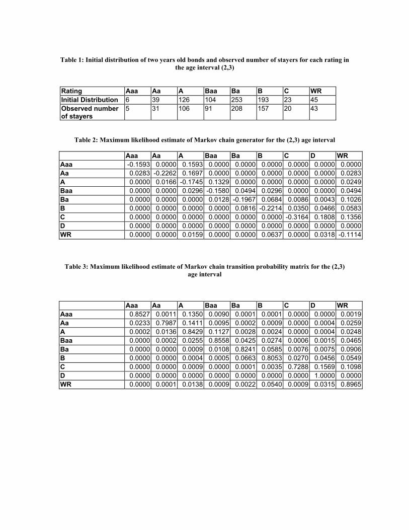
Table 1: Initial distribution of two years old bonds and observed number of stayers for each rating in

the age interval (2,3)

Rating Aaa Aa A Baa Ba B C WR Initial Distribution 6 39 126 104 253 193 23 45 Observed number of stayers

5 31 106 91 208 157 20 43

Table 2: Maximum likelihood estimate of Markov chain generator for the (2,3) age interval

Aaa Aa A Baa Ba B C D WR Aaa -0.1593 0.0000 0.1593 0.0000 0.0000 0.0000 0.0000 0.0000 0.0000Aa 0.0283 -0.2262 0.1697 0.0000 0.0000 0.0000 0.0000 0.0000 0.0283A 0.0000 0.0166 -0.1745 0.1329 0.0000 0.0000 0.0000 0.0000 0.0249Baa 0.0000 0.0000 0.0296 -0.1580 0.0494 0.0296 0.0000 0.0000 0.0494Ba 0.0000 0.0000 0.0000 0.0128 -0.1967 0.0684 0.0086 0.0043 0.1026B 0.0000 0.0000 0.0000 0.0000 0.0816 -0.2214 0.0350 0.0466 0.0583C 0.0000 0.0000 0.0000 0.0000 0.0000 0.0000 -0.3164 0.1808 0.1356D 0.0000 0.0000 0.0000 0.0000 0.0000 0.0000 0.0000 0.0000 0.0000WR 0.0000 0.0000 0.0159 0.0000 0.0000 0.0637 0.0000 0.0318 -0.1114

Table 3: Maximum likelihood estimate of Markov chain transition probability matrix for the (2,3) age interval

Aaa Aa A Baa Ba B C D WR

Aaa 0.8527 0.0011 0.1350 0.0090 0.0001 0.0001 0.0000 0.0000 0.0019Aa 0.0233 0.7987 0.1411 0.0095 0.0002 0.0009 0.0000 0.0004 0.0259A 0.0002 0.0136 0.8429 0.1127 0.0028 0.0024 0.0000 0.0004 0.0248Baa 0.0000 0.0002 0.0255 0.8558 0.0425 0.0274 0.0006 0.0015 0.0465Ba 0.0000 0.0000 0.0009 0.0108 0.8241 0.0585 0.0076 0.0075 0.0906B 0.0000 0.0000 0.0004 0.0005 0.0663 0.8053 0.0270 0.0456 0.0549C 0.0000 0.0000 0.0009 0.0000 0.0001 0.0035 0.7288 0.1569 0.1098D 0.0000 0.0000 0.0000 0.0000 0.0000 0.0000 0.0000 1.0000 0.0000WR 0.0000 0.0001 0.0138 0.0009 0.0022 0.0540 0.0009 0.0315 0.8965

Table 4: Maximum likelihood etimates of the proportion of “stayers” in the (2,3) age interval

Rating Aaa Aa A Baa Ba B C WR si 0 0 0.11 0.56 0 0.07 0.81 0.75

Table 5: Maximum likelihood estimate of the generator for the movers in the (2,3) age interval

Aaa Aa A Baa Ba B C D WR Aaa -0.1594 0.0000 0.1594 0.0000 0.0000 0.0000 0.0000 0.0000 0.0000Aa 0.0283 -0.2268 0.1701 0.0000 0.0000 0.0000 0.0000 0.0000 0.0283A 0.0000 0.0187 -0.1967 0.1499 0.0000 0.0000 0.0000 0.0000 0.0281Baa 0.0000 0.0000 0.0660 -0.3522 0.1101 0.0660 0.0000 0.0000 0.1101Ba 0.0000 0.0000 0.0000 0.0129 -0.1972 0.0686 0.0086 0.0043 0.1029B 0.0000 0.0000 0.0000 0.0000 0.0877 -0.2379 0.0376 0.0501 0.0626C 0.0000 0.0000 0.0000 0.0000 0.0000 0.0000 -1.3100 0.7486 0.5614D 0.0000 0.0000 0.0000 0.0000 0.0000 0.0000 0.0000 0.0000 0.0000WR 0.0000 0.0000 0.0314 0.0000 0.0000 0.1256 0.0000 0.0628 -0.2197 Table 6: Maximum likelihood estimate of transition probability matrix of the mover - stayer model in

the (2,3) age interval

Aaa Aa A Baa Ba B C D WR

Aaa 0.8527 0.0012 0.1336 0.0094 0.0004 0.0003 0.0000 0.0001 0.0022Aa 0.0233 0.7988 0.1399 0.0099 0.0004 0.0017 0.0000 0.0008 0.0250A 0.0002 0.0135 0.8458 0.1019 0.0059 0.0051 0.0001 0.0009 0.0266Baa 0.0000 0.0002 0.0227 0.8715 0.0379 0.0254 0.0005 0.0022 0.0396Ba 0.0000 0.0000 0.0017 0.0099 0.8246 0.0608 0.0050 0.0106 0.0874B 0.0000 0.0000 0.0008 0.0004 0.0661 0.8078 0.0172 0.0519 0.0557C 0.0000 0.0000 0.0010 0.0001 0.0001 0.0039 0.8594 0.0826 0.0530D 0.0000 0.0000 0.0000 0.0000 0.0000 0.0000 0.0000 1.0000 0.0000WR 0.0000 0.0001 0.0063 0.0005 0.0011 0.0247 0.0003 0.0147 0.9524

Tables 7a-c: One-year default probabilities from ratings C, B and Ba using mover - stayer and Markov chain models.

Table 7a

C-->D Year Markov Chain Mover - Stayer Model Proportion of

Stayers in C 1 0.0000 0.0000 0.88 2 0.1920 0.1153 0.77 3 0.1569 0.0826 0.81 4 0.1000 0.0737 0.81 5 0.2118 0.1892 0.43

Table 7b

B-->D Year Markov Chain Model Mover - Stayer Model Proportion of

Stayers in B 1 0.0039 0.0039 0.15 2 0.0379 0.0435 0.3 3 0.0456 0.0519 0.07 4 0.1006 0.1038 0.13 5 0.1173 0.1189 0

Table 7c

Ba-->D Year Markov Chain Model Mover - Stayer Model Proportion of

Stayers in Ba 1 0.0000 0.0000 0.86 2 0.0379 0.0064 0 3 0.0075 0.0106 0 4 0.0202 0.0214 0 5 0.0077 0.0088 0