Estimation and Forecasting in Models with Multiple

Breaks�

Gary Koopyand Simon M. Potterz

November 2004, revised September 2006

Abstract

This paper develops a new approach to change-point modeling thatallows the number of change-points in the observed sample to be un-known. The model we develop assumes regime durations have a Pois-son distribution. It approximately nests the two most common ap-proaches: the time varying parameter model with a change-point everyperiod and the change-point model with a small number of regimes.We focus considerable attention on the construction of reasonable hier-archical priors both for regime durations and for the parameters whichcharacterize each regime. A Markov Chain Monte Carlo posterior sam-pler is constructed to estimate a version of our model which allows forchange in conditional means and variances. We show how real timeforecasting can be done in an e¢ cient manner using sequential impor-tance sampling. Our techniques are found to work well in an empiricalexercise involving US GDP growth and in�ation. Empirical resultssuggest that the number of change-points is larger than previouslyestimated in these series and the implied model is similar to a timevarying parameter (with stochastic volatility) model.JEL classi�cation: C11, C22, E17Keywords: Bayesian, structural break, Markov Chain Monte Carlo,

hierarchical prior, sequential importance sampling

�We would like to thank Paolo Giordani, Edward Leamer, Richard Paap, HashemPesaran, Herman van Dijk, two referees, the editor and seminar participants at theSwedish Central Bank, the Federal Reserve Bank of St. Louis, Erasmus Universityand the Universities of Amsterdam, Kansas and York for helpful comments. Theviews expressed in this paper are those of the authors and do not necessarily re�ectthe views of the Federal Reserve Bank of New York or the Federal Reserve System.

yDepartment of Economics, University of Strathclyde, Glasgow U.K.,Gary.Koop@strath.ac.uk

zFederal Reserve Bank of New York, Simon.Potter@ny.frb.org

1

1 Introduction

Many recent papers have highlighted the fact that structural instabilityseems to be present in a wide variety of macroeconomic and �nancial timeseries [e.g. Ang and Bekaert (2002) and Stock and Watson (1996)]. Thenegative consequences of ignoring this instability for inference and forecast-ing has been stressed by, among many others, Clements and Hendry (1998,1999), Koop and Potter (2001) and Pesaran, Pettenuzzo and Timmerman(2006). This has inspired a wide range of change-point models. There aretwo main approaches: one can estimate a model with a small number ofchange-points (usually one or two). Alternatively, one can estimate a timevarying parameter (TVP) model where the parameters are allowed to changewith each new observation, usually according to a random walk. A TVPmodel can be interpreted as having T�1 breaks in a sample of size T . Recentin�uential empirical work includes McConnell and Perez (2000) who use asingle change-point model to present evidence that the volatility of US eco-nomic activity abruptly fell in early 1984. In a TVP framework, Cogley andSargent (2001) model in�ation dynamics in the US as continuously evolvingover time.

Models with a small number of structural breaks typically do not re-strict the magnitude of change in the coe¢ cients that can happen after abreak, but implicitly assume that after the last break is estimated in thesample there will be no more breaks. In contrast, in the TVP model thereis probability 1 of a break in the next new observation. However, for theTVP model the size of the break is severely limited by the assumption thatcoe¢ cients evolve according to a random walk.

The previous paragraphs highlight the two main issues which must beaddressed when building a change-point model: how to model the durationof each regime and how to model the change in coe¢ cients after a breakoccurs. In this paper, we develop a new model which, we argue addressesboth of these issues in a empirically-sensible manner. For reasons outlinedbelow, we use Bayesian methods. The model we develop draws on our beliefsthat desirable features for a change-point model are:

1. The number of regimes and their maximum duration should not berestricted ex-ante.

2. The regime duration distribution should not be restricted to be con-stant or monotonically decreasing/increasing.

3. The parameters describing the distribution of the parameters in each

2

regime should, if possible, have conditionally conjugate prior distribu-tions to minimize the computational complexity of change-point mod-els.

4. Durations of previous regimes can potentially provide some informa-tion about durations of future regimes.

5. The parameters characterizing a new regime can potentially dependon the parameters of the old regime.

6. The change-point model should be easy to update in real time as newdata arrives on the time series of interest.

It can immediately be seen that standard implementations of the TVPmodel and models with small numbers of breaks do not have these features.Furthermore, as we shall see, common Bayesian approaches to these models(which augment standard implementations with hierarchical priors) also donot have these features.

Bayesian methods are attractive for change-point models since they canallow for �exible relationships between parameters in various regimes andare computationally simple. That is, in a model with M > 1 regimes, hi-erarchical priors can be used to allow information about coe¢ cients in thejth regime (or the duration of the jth regime) to depend on information inthe other regimes. Such an approach can improve estimation of coe¢ cients.It is particularly useful for forecasting in the presence of structural breakssince it allows for the possibility of out-of-sample breaks. That is, in themodel we develop, a new break can be forecast after the end of the sampleand size of the break is partly dependent on the properties of the previousregime, partly dependent on the history of all previous breaks and partlyhas a random element. With regards to computation, use of a hierarchicalprior allows the researcher to structure the model so that, conditional on un-known parameters (e.g. the change-points) or a vector of latent data (e.g. astate vector denoting the regimes), it is very simple (e.g. a series of Normallinear regression models). E¢ cient Markov Chain Monte Carlo (MCMC)algorithms which exploit this structure can be developed. This allows forthe estimation of models, using modern Bayesian methods, with multiplechange-points that are di¢ cult under the standard classical approach tochange-point problems. However, with some partial exceptions [e.g. Chib(1998), Pesaran, Pettenuzzo and Timmerman (2006) and Stambaugh andPastor (2001)], we would argue that the existing Bayesian literature in eco-nomics has not fully exploited the bene�ts of using hierarchical priors. In

3

addition, this literature has, following the existing frequentist literature, fo-cussed on either models with a small number of breaks or TVP models.Furthermore, as argued in Koop and Potter (2004), some commonly-usedBayesian priors have undesirable properties.

The plan of this paper is as follows. In Section 2 we review the linkbetween change-points and hidden Markov chains. In Section 3 we developour new model of regime duration. In Section 4 we construct a method formodeling the change in regime coe¢ cients based on a similar hierarchicalstructure to the TVP model. Section 5 gives an overview of the posteriorsimulator used in our Bayesian analysis.1 This section also shows how se-quential importance sampling (i.e. particle �ltering2) methods can be usedwith our model to carry out real time forecasting in a computationally ef-�cient manner. Section 6 contains applications to US GDP growth andin�ation as measured by the PCE de�ator. We compare the results of ourapproach with that of a single structural break and a TVP model and �ndthem to be closer to the latter. In general, we �nd our methods to reli-ably recover key data features without making the potentially restrictiveassumptions underlying other popular models.

2 Change-Point Models and HiddenMarkov Chains

In order to discuss the advantages of our model, it is worthwhile to beginby describing in detail some recent work and, in particular, the innova-tive model of Chib (1998) which has been used in many applications [e.g.Pastor and Stambaugh (2001), Kim, Nelson and Piger (2002) and Pesaran,Pettenuzzo and Timmerman (2006)].3 In terms of computation, our focusis on extending Chib�s insight of converting the classical change-point prob-lem into a Markov mixture model and using the algorithm of Chib (1996)to estimate the change-points and the parameters within each regime.

We have data on a scalar time series variable, yt for t = 1; : : : ; T andlet Yi = (y1; : : : ; yi)

0 denote the history through time i and denote thefuture by Y i+1 = (yi+1; : : : ; yT )

0. Regime changes depend upon a dis-

1Complete details are provided in the working paper version with title "Forecasting andEstimating Multiple Change-point Models with an Unknown Number of Change-points"available at http://personal.strath.ac.uk/gary.koop/.

2Particle �ltering is sequential importance sampling with resampling. For our purposes,resampling is not required (although we describe how it can be done).

3 In contrast, a recent in�uential Bayesian paper, Maheu and Gordon (2005), does notapply such a hiearchical prior structure and, thus, is not directly comparable to the papersdiscussed in this section.

4

crete random variable, st, which takes on values f1; 2; : : : ;Mg. We letSi = (s1; : : : ; si)

0 and Si+1 = (si+1; : : : ; sT )0. The likelihood function is

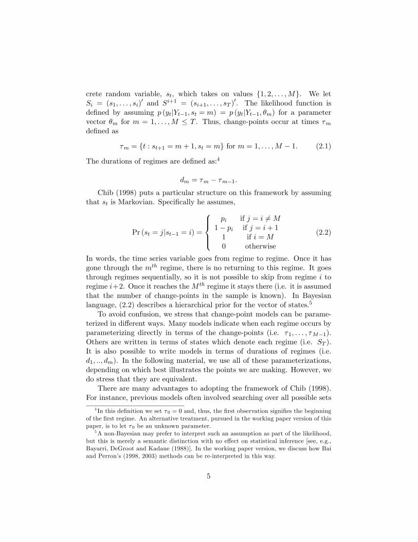
de�ned by assuming p (ytjYt�1; st = m) = p (ytjYt�1; �m) for a parametervector �m for m = 1; : : : ;M � T . Thus, change-points occur at times �mde�ned as

�m = ft : st+1 = m+ 1; st = mg for m = 1; : : : ;M � 1: (2.1)

The durations of regimes are de�ned as:4

dm = �m � �m�1:Chib (1998) puts a particular structure on this framework by assuming

that st is Markovian. Speci�cally he assumes,

Pr (st = jjst�1 = i) =

8>><>>:pi if j = i 6=M

1� pi if j = i+ 11 if i =M0 otherwise

(2.2)

In words, the time series variable goes from regime to regime. Once it hasgone through the mth regime, there is no returning to this regime. It goesthrough regimes sequentially, so it is not possible to skip from regime i toregime i+2. Once it reaches theM th regime it stays there (i.e. it is assumedthat the number of change-points in the sample is known). In Bayesianlanguage, (2.2) describes a hierarchical prior for the vector of states.5

To avoid confusion, we stress that change-point models can be parame-terized in di¤erent ways. Many models indicate when each regime occurs byparameterizing directly in terms of the change-points (i.e. �1; : : : ; �M�1).Others are written in terms of states which denote each regime (i.e. ST ).It is also possible to write models in terms of durations of regimes (i.e.d1; ::; dm). In the following material, we use all of these parameterizations,depending on which best illustrates the points we are making. However, wedo stress that they are equivalent.

There are many advantages to adopting the framework of Chib (1998).For instance, previous models often involved searching over all possible sets

4 In this de�nition we set �0 = 0 and, thus, the �rst observation signi�es the beginningof the �rst regime. An alternative treatment, pursued in the working paper version of thispaper, is to let �0 be an unknown parameter.

5A non-Bayesian may prefer to interpret such an assumption as part of the likelihood,but this is merely a semantic distinction with no e¤ect on statistical inference [see, e.g.,Bayarri, DeGroot and Kadane (1988)]. In the working paper version, we discuss how Baiand Perron�s (1998, 2003) methods can be re-interpreted in this way.

5

of break points. If the number of break points is even moderately large, thencomputational costs can become overwhelming [see, for instance, the discus-sion in Elliott and Muller (2006)]. By using the Markov mixture model,the posterior simulator is recovering information on the most likely change-points given the sample and the computational burden is greatly lowered,making it easy to estimate models with many change-points. Appendix Adescribes this algorithm (which we use, with modi�cations, as a componentof the posterior simulator for our model).

Chib chose to model the states� transition probabilities as being con-stants. One consequence of this is that regime duration satis�es a Geomet-ric distribution, a possibly restrictive choice. For instance, the Geometricdistribution is decreasing, implying that p (dm) > p (dm + 1) which (in someapplications) may be unreasonable. In the model we introduce below, wegeneralize this restriction by allowing regime duration to follow a more �ex-ible Poisson distribution.

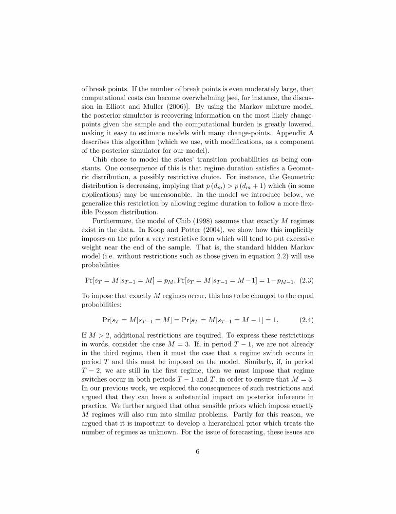
Furthermore, the model of Chib (1998) assumes that exactly M regimesexist in the data. In Koop and Potter (2004), we show how this implicitlyimposes on the prior a very restrictive form which will tend to put excessiveweight near the end of the sample. That is, the standard hidden Markovmodel (i.e. without restrictions such as those given in equation 2.2) will useprobabilities

Pr[sT =M jsT�1 =M ] = pM ;Pr[sT =M jsT�1 =M�1] = 1�pM�1: (2.3)

To impose that exactlyM regimes occur, this has to be changed to the equalprobabilities:

Pr[sT =M jsT�1 =M ] = Pr[sT =M jsT�1 =M � 1] = 1: (2.4)

If M > 2, additional restrictions are required. To express these restrictionsin words, consider the case M = 3. If, in period T � 1, we are not alreadyin the third regime, then it must the case that a regime switch occurs inperiod T and this must be imposed on the model. Similarly, if, in periodT � 2, we are still in the �rst regime, then we must impose that regimeswitches occur in both periods T � 1 and T , in order to ensure that M = 3.In our previous work, we explored the consequences of such restrictions andargued that they can have a substantial impact on posterior inference inpractice. We further argued that other sensible priors which impose exactlyM regimes will also run into similar problems. Partly for this reason, weargued that it is important to develop a hierarchical prior which treats thenumber of regimes as unknown. For the issue of forecasting, these issues are

6

even more important, since these prior restrictions occur at the end of thesample, precisely where forecasting begins.

Chib (1998) did not consider the question of out-of-sample forecasting.If one were to assume no additional breaks occur out-of-sample, forecastingcould be done in a straightforward fashion, based on the likelihood and priorwhich hold at the end of the sample (i.e. p (yT jYT�1; �M ) and p (�M )). Suchan approach, of course, does not address the issue of forecasting when breakscan occur out of sample. Pesaran, Pettenuzzo and Timmerman (2006) tookup the challenge of extending the Chib approach to address this latter issue.They assume a constant transition probability matrix out-of-sample whichallows for a probability of a break occurring in each out-of-sample period.Their approach is attractive and, in many ways, a sensible one. However, inadapting the approach of Chib (1998) in this manner, some problems arise.Remember that, to impose exactlyM regimes in-sample, restrictions such as(2.4) must be imposed. But, out-of-sample, to allow for breaks to occur, itis desirable to revert to an unrestricted transition probability such as (2.3).Pesaran, Pettenuzzo and Timmerman (2006) explicitly assume that

P [st =M jst�1 =M ] =�

1 if t � TpM if t > T

; (2.5)

with the restriction that P [sT =M ] = 1: This assumption, since it is at theend of sample, could conceivably have an important in�uence on forecasting.To try and understand this assumption better, consider what would happenif we increase the observed sample by one observation. Most Bayesians wouldargue that any statistical procedure for updating in response to the additionof an extra observation should satisfy Bayes�rule. However, the updatingof Pesaran, Pettenuzzo and Timmerman (2006) with an extra observationcould be taken to imply:

P [st =M jst�1 =M ] =�

1 if t � T + 1pM if t > T + 1

; P [sT+1 =M ] = 1;

which is inconsistent with (2.5) and violates Bayes�Rule.These problems arise due to the imposition of exactly M breaks in-

sample. Pesaran, Pettenuzzo and Timmerman (2006) partly address thisproblem through considering models with di¤erent values for M and thendoing Bayesian model averaging. This is a sensible thing to do, but doesnot fully address the problems noted above (i.e. a pile-up of probabilitynear the end of the sample and the di¢ culty in adapting the approach toout-of-sample forecasting in a way which does not violate Bayes�rule). In

7

the next section, we will propose our model which does not impose a �xednumber of breaks in-sample and, hence, does not run into these problems.

Another relevant paper is McCulloch and Tsay (1993). The model usedin this paper is di¤erent in many ways from Chib (1998) and Pesaran, Pet-tenuzzo and Timmerman (2006). However, it does have regimes changingwith a certain probability. McCulloch and Tsay do not assume a �xed num-ber of breaks and do not face the problems noted above since they assumethat the probability of a break occurring is constant for all observations (inan extension, they allow this probability to depend on additional covariates).In essence, whereas Chib (1998) allows the probability of a break in regime jto be pj , in McCulloch and Tsay (1993) this is simpli�ed to a single p. Thisp can be estimated in-sample and then used in out-of-sample forecasting,thus precluding the need for an assumption such as (2.5). However, the as-sumption of a time- and regime-invariant transition probability is restrictivein many macroeconomic contexts. Furthermore, it will share many of therestrictive features of Chib (1998). For instance, the hierarchical prior forregime duration will be a Geometric distribution.

In summary, the pioneering work of Chib (1998) followed by the workof Pesaran, Pettenuzzo and Timmerman (2006) has changed the way manylook at change-point models. Both papers have had great in�uence and havemany attractive features. In terms of posterior computation, Chib (1998)continues to be very attractive and, indeed, we use a modi�cation of thisalgorithm as part of our posterior simulator. However, the hierarchical priorhas some potentially undesirable properties which leads us to want to buildon these previous approaches.

3 A Poisson Hierarchical Prior for Durations

The previous discussion illustrates some restrictive properties of traditionalhierarchical priors used in the change-point literature and leads to our con-tention that it is desirable to have a model for durations which satis�es thesix criteria listed in the introduction. In this section we develop our alter-native approach based on a Poisson model for durations.6 This approachdoes not restrict the number or maximum durations of regimes ex-ante, ithas a convenient conjugate prior distribution in the Gamma family and the

6Of course, there are many other popular options for modeling durations other thanthe Poisson. Bracqemond and Gaudoin (2003) o¤ers a good categorization of di¤erentpossibilities and explains their properties. Our methods could be extended to deal withany of these in a straightforward manner.

8

regime duration distribution is not restricted to be constant or monotoni-cally decreasing/increasing. It also allows information about the durationof past regimes to a¤ect the duration of the current regime and potentiallythe magnitude of the parameter change from old to new regime.

We use a hierarchical prior for the regime durations which is a Poissondistribution. That is, p (dmj�m) is given by:

dm � 1 = �m � (�m�1 + 1) � Po(�m) (3.1)

where Po(�m) denotes the Poisson distribution with mean �m. With thishierarchical prior it makes sense to use a (conditionally conjugate) Gammaprior on �m. If we do this, it can be veri�ed that p (dm), the marginal priorfor the duration between change points, is given by a Negative Binomialdistribution.

To provide some intuition, remember that the assumption comparableto (3.1) in the model of Chib (1998) was that the duration had a hierarchicalprior which was Geometric (apart from the end-points). Chib (1998) used aBeta prior on the parameters. This hierarchical prior [and, as shown in Koopand Potter (2004), the marginal prior p (dm)] implies a declining probabilityon regime duration so that higher weight is placed on shorter durations. Incontrast, the Poisson form we use for p (dmj�m) and the implied NegativeBinomial form for p (dm) which we work with have no such restriction.

However, the prior given in (3.1) also has the unconventional propertythat it allocates prior weight to change-points outside the observed sample.That is, there is nothing in (3.1) which even restricts d1 < T much lessdm < T for m > 1. We will argue that this is a highly desirable propertysince, not only does this prior not place excessive weight on change-pointsnear the end of the sample, but also there is a sense in which it allows us tohandle the case where there is an unknown number of change-points. Thatis, suppose we allow for m = 1; :::;M regimes. Then, since some or all of theregimes can terminate out-of-sample, our model implicitly contains modelswith no breaks, one break, up to M � 1 breaks (in-sample).7 The desirableproperties of this feature are explored in more detail in Koop and Potter(2004).8

7The speci�cation of a maximum number of regimes, M , is made only for illustrativepurposes. In practice, our model does not require speci�cation of such a maximum. Inour empirical work we set M = T which allows for anything up to a TVP model and anout-of-sample break.

8 In a di¤erent but related context (i.e. a Markov switching model), Chopin and Pelgrin(2004), adopt a di¤erent approach to the joint estimation of number of regimes and theparameters.

9

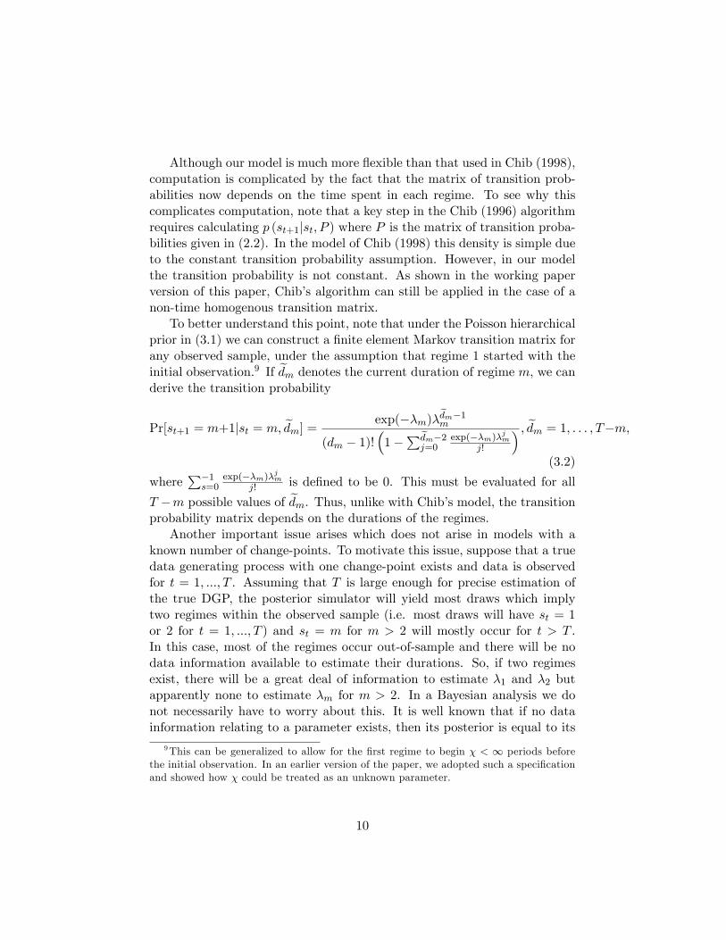
Although our model is much more �exible than that used in Chib (1998),computation is complicated by the fact that the matrix of transition prob-abilities now depends on the time spent in each regime. To see why thiscomplicates computation, note that a key step in the Chib (1996) algorithmrequires calculating p (st+1jst; P ) where P is the matrix of transition proba-bilities given in (2.2). In the model of Chib (1998) this density is simple dueto the constant transition probability assumption. However, in our modelthe transition probability is not constant. As shown in the working paperversion of this paper, Chib�s algorithm can still be applied in the case of anon-time homogenous transition matrix.

To better understand this point, note that under the Poisson hierarchicalprior in (3.1) we can construct a �nite element Markov transition matrix forany observed sample, under the assumption that regime 1 started with theinitial observation.9 If edm denotes the current duration of regime m, we canderive the transition probability

Pr[st+1 = m+1jst = m; edm] = exp(��m)�edm�1m

(dm � 1)!�1�

Pedm�2j=0

exp(��m)�jmj!

� ; edm = 1; : : : ; T�m;(3.2)

whereP�1s=0

exp(��m)�jmj! is de�ned to be 0. This must be evaluated for all

T �m possible values of edm. Thus, unlike with Chib�s model, the transitionprobability matrix depends on the durations of the regimes.

Another important issue arises which does not arise in models with aknown number of change-points. To motivate this issue, suppose that a truedata generating process with one change-point exists and data is observedfor t = 1; :::; T . Assuming that T is large enough for precise estimation ofthe true DGP, the posterior simulator will yield most draws which implytwo regimes within the observed sample (i.e. most draws will have st = 1or 2 for t = 1; :::; T ) and st = m for m > 2 will mostly occur for t > T .In this case, most of the regimes occur out-of-sample and there will be nodata information available to estimate their durations. So, if two regimesexist, there will be a great deal of information to estimate �1 and �2 butapparently none to estimate �m for m > 2. In a Bayesian analysis we donot necessarily have to worry about this. It is well known that if no datainformation relating to a parameter exists, then its posterior is equal to its

9This can be generalized to allow for the �rst regime to begin � < 1 periods beforethe initial observation. In an earlier version of the paper, we adopted such a speci�cationand showed how � could be treated as an unknown parameter.

10

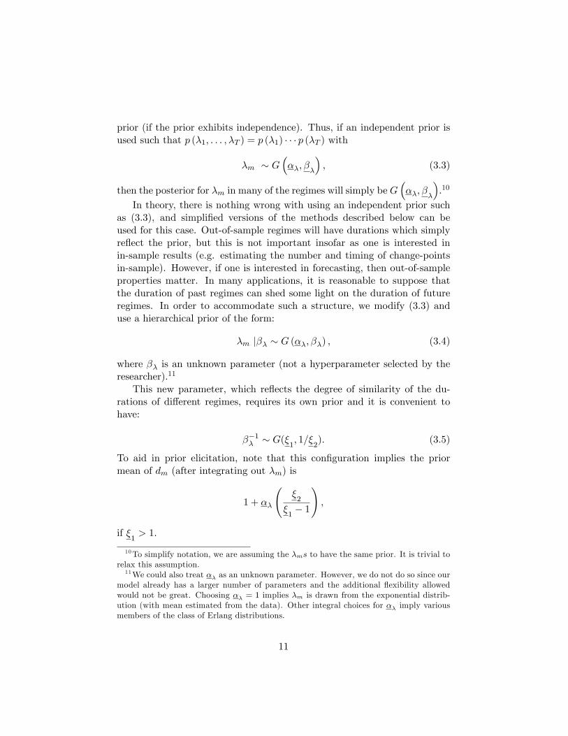
prior (if the prior exhibits independence). Thus, if an independent prior isused such that p (�1; : : : ; �T ) = p (�1) � � � p (�T ) with

�m � G���; ��

�; (3.3)

then the posterior for �m in many of the regimes will simply be G���; ��

�.10

In theory, there is nothing wrong with using an independent prior suchas (3.3), and simpli�ed versions of the methods described below can beused for this case. Out-of-sample regimes will have durations which simplyre�ect the prior, but this is not important insofar as one is interested inin-sample results (e.g. estimating the number and timing of change-pointsin-sample). However, if one is interested in forecasting, then out-of-sampleproperties matter. In many applications, it is reasonable to suppose thatthe duration of past regimes can shed some light on the duration of futureregimes. In order to accommodate such a structure, we modify (3.3) anduse a hierarchical prior of the form:

�m j�� � G (��; ��) ; (3.4)

where �� is an unknown parameter (not a hyperparameter selected by theresearcher).11

This new parameter, which re�ects the degree of similarity of the du-rations of di¤erent regimes, requires its own prior and it is convenient tohave:

��1� � G(�1; 1=�

2): (3.5)

To aid in prior elicitation, note that this con�guration implies the priormean of dm (after integrating out �m) is

1 + ��

�2

�1� 1

!;

if �1> 1:

10To simplify notation, we are assuming the �ms to have the same prior. It is trivial torelax this assumption.11We could also treat �� as an unknown parameter. However, we do not do so since our

model already has a larger number of parameters and the additional �exibility allowedwould not be great. Choosing �� = 1 implies �m is drawn from the exponential distrib-ution (with mean estimated from the data). Other integral choices for �� imply variousmembers of the class of Erlang distributions.

11

It is important to understand the implications of any prior (the appen-dix discusses such properties by simulating from the particular prior usedin our empirical work). As discussed following (3.1), we propose a hierar-chical prior where p (dmj�m) is Poisson, but if we integrate out �m, we getp (dmj��) being a Negative Binomial distribution. The unconditional priordistribution, p (dm) is found by integrating out ��1� . This does not have aclosed form.12 In general p (dm) inherits the �exible form of p (dmj�m) orp (dmj��). However, it is worth mentioning that if �� = 1 then we havethe restrictive property that P (dm = y) > P (dm = y + 1). This suggeststhat, for most applications, it is desirable to avoid such small values for ��.It can also be shown that, by suitable choice of �

1and �

2; with �� = n

we have a high prior probability of a regime change every n periods. Suchconsiderations can be useful in prior elicitation.

In summary, in this section we have developed a hierarchical prior forthe regime durations which has two levels to the hierarchy. At the �rst level,we assume the durations to have Poisson distributions. At the second level,we assume the Poisson intensities (i.e. �ms) are drawn from a common dis-tribution. Thus, out-of-sample �ms (and, thus, regime durations) are drawnfrom this common distribution (which is estimated using in-sample data).This is important for forecasting as it allows for the predictive distributionto re�ect the possibility that a change-point occurs during the period beingforecast.

4 Development of the Prior for the Parameters inEach Regime

In the same way that the change-point framework of Chib (1998) can be usedwith a wide variety of likelihoods (i.e. p (ytjYt�1; st = m) can have manyforms), our Poisson model for durations can be used with any speci�cationfor p (ytjYt�1; st = m) = p (ytjYt�1; �m). Here we choose a particular struc-ture based on a regression or autoregressive model with stochastic volatilitywhich is of empirical relevance.

Many change-point models assume that the anything can happen to theparameters after a regime change occurs. The issues which arise with suchan approach are elegantly expressed by Pastor and Stambaugh (2001) in anapplication which used stock return data to investigate the equity premium.

12The working paper version of this paper contains an expression for it that could beevaluated numerically.

12

"In standard approaches to models that admit structural breaks,estimates of current parameters rely on data only since the mostrecent estimated break. Discarding the earlier data reduces therisk of contaminating an estimate of the equity premium withdata generated under a di¤erent [process]. That practice seemsprudent, but it contends with the reality that shorter historiestypically yield less precise estimates. Suppose... a shift in theequity premium occurred a month ago. Discarding virtually allof the historical data on equity returns would certainly removethe risk of contamination by pre-break data, but it hardly seemssensible in estimating the current equity premium. Completelydiscarding the pre-break data is appropriate only when the pre-mium might have shifted to such a degree that the pre-breakdata are no more useful ..., than, say, pre-break rainfall data,but such a view almost surely ignores economics." Pastor andStambaugh (2001, pages 1207-1208).

The case for adopting a hierarchical prior which allows for some sort oflink between pre- and post-break parameters is, we believe, compelling inmany empirical contexts. The question arises as to what sort of hierarchicalprior is appropriate. We adopt a state space framework where the observabletime series satis�es the measurement equation

yt = Xt�st + exp(�st=2)"t; (4.1)

where "t � N(0; 1) and the (K+1) state vector �st = f�st ; �stg satis�es thestate transition equations

�m = �m�1 + Um; (4.2)

�m = �m�1 + um;

where Um � N(0; V ), um � N(0; �) and Xt is a K-dimensional row vectorcontaining lagged dependent or other explanatory variables. The initialconditions, �0 and �0 can be treated in the same way as in any state spacealgorithm.13

Note that this framework di¤ers from a standard state space model usedin TVP formulations in that the subscripts on the parameters of the mea-surement equation do not have t subscripts, but rather st subscripts so that

13 In particular, in our state space algorithm the forward �lter step is initialized with adi¤use prior.

13

parameters change only when states change. This di¤erence leads to thestate equations having m subscripts to denote the m = 1; :::;M regimes.

To draw out the contrasts with models with a small number of breaks,note that the hierarchical prior in (4.2) assumes that �m depends on �m�1.A similar approach is adopted in McCulloch and Tsay (1993) for the in-tercept and error variance in an autoregressive model. In most traditionalmodels with a small number of breaks, one assumes �m and �m�1 are in-dependent of one another [e.g. Chib (1998) or Maheu and Gordon (2005)].Furthermore, it is usually assumed that the priors come from a conjugatefamily. For instance, a traditional model might begin with (4.1) and thenlet �m have the same Normal-Gamma natural conjugate prior for all m.This approach, involving unconditionally independent priors, is not reason-able in our model for reasons we have partially discussed above. That is,our approach involves an unknown number of change-points in the observedsample. So it is possible that many of the regimes occur out-of-sample. Intraditional formulations, there is no data information to estimate �m if themth regime occurs out-of-sample. The hierarchical prior of (4.2) alleviatesthis problem. An alternative approach to this issue is given in Pastor andStambaugh (2001) and Pesaran, Pettenuzzo and Timmerman (2006). Theyplace a hierarchy on the parameters of the conjugate family for each regime.For instance, Pesaran, Pettenuzzo and Timmerman (2006) assume that allthe �ms are drawn from a common distribution. This is a standard approachin the Bayesian literature for cross-section data drawn from di¤erent groups.In a time series applications it has less merit since one wants the most recentregimes to have the strongest in�uence on the new regime. This is a featurethat our hierarchical prior incorporates.

The state equations in (4.2) de�ne a hierarchical prior which links �mand �m�1 in a sensible way. This martingale structure is standard in theTVP literature and, as we discuss later, it is computationally simple since itallows the use of standard Kalman �lter and smoother techniques to drawthe parameters in each regime. We use a standard (conditionally conjugate)prior for the innovation variances:

V �1 � W�V �1V ; �V

�(4.3)

��1 � G(��; ��)

whereW (A; a) denotes the Wishart distribution14 and we assume that �V >K + 1.14We parameterize the Wishart distribution so that if Z � W (A; a) and ij subscripts

14

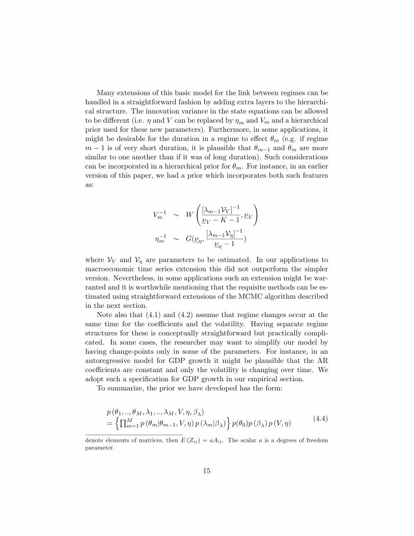
Many extensions of this basic model for the link between regimes can behandled in a straightforward fashion by adding extra layers to the hierarchi-cal structure. The innovation variance in the state equations can be allowedto be di¤erent (i.e. � and V can be replaced by �m and Vm and a hierarchicalprior used for these new parameters). Furthermore, in some applications, itmight be desirable for the duration in a regime to e¤ect �m (e.g. if regimem � 1 is of very short duration, it is plausible that �m�1 and �m are moresimilar to one another than if it was of long duration). Such considerationscan be incorporated in a hierarchical prior for �m. For instance, in an earlierversion of this paper, we had a prior which incorporates both such featuresas:

V �1m � W

[�m�1VV ]�1

�V �K � 1 ; �V

!

��1m � G(��;[�m�1V�]�1

�� � 1)

where VV and V� are parameters to be estimated. In our applications tomacroeconomic time series extension this did not outperform the simplerversion. Nevertheless, in some applications such an extension might be war-ranted and it is worthwhile mentioning that the requisite methods can be es-timated using straightforward extensions of the MCMC algorithm describedin the next section.

Note also that (4.1) and (4.2) assume that regime changes occur at thesame time for the coe¢ cients and the volatility. Having separate regimestructures for these is conceptually straightforward but practically compli-cated. In some cases, the researcher may want to simplify our model byhaving change-points only in some of the parameters. For instance, in anautoregressive model for GDP growth it might be plausible that the ARcoe¢ cients are constant and only the volatility is changing over time. Weadopt such a speci�cation for GDP growth in our empirical section.

To summarize, the prior we have developed has the form:

p (�1; ::; �M ; �1; ::; �M ; V; �; ��)

=nQM

m=1 p (�mj�m�1; V; �) p (�mj��)op(�0)p (��) p (V; �)

(4.4)

denote elements of matrices, then E (Zij) = aAij . The scalar a is a degrees of freedomparameter.

15

where p (�mj�m�1; V; �) is given by (4.2), p(�0) is di¤use, (V; �) is given by(4.3), p (�mj��) is given by (3.4) and p (��) is given by (3.5).

5 Posterior and Predictive Simulation

In this section we outline the general form of the MCMC algorithm used toestimate the model. Precise details are provided in the working paper versionof this paper.15 To simplify notation we de�ne � =

��01; :::; �

0M

�0 and � =��01; :::; �

0M

�0. Note that our MCMC algorithm draws a sequence of states(ST ) that implies the values for the regime durations, dm. Furthermore, wewill set M = T so that we can nest a standard TVP model. However, itis possible to set M < T if one wishes to restrict the number of feasibleregimes.

Our MCMC proceeds by sequentially drawing from the full posteriorconditionals for the parameters ST ; �; �; V; �; ��. The posterior conditionalp (ST jYT ;�; �; V; �; ��) = p (ST jYT ;�; �) can be drawn using the modi-�ed algorithm of Chib (1996) with transition probabilities given by (3.2).p (�jYT ; ST ; �; V; �; ��) can be simulated using extensions of methods of pos-terior simulation for state space models with stochastic volatility drawingon Kim, Shephard and Chib (1998) and Carter and Kohn (1994). That is,the TVP model is a standard state space model and thus, standard statespace simulation methods can be used directly. However, when regimes lastmore than one period, the simulator has to be altered in a straightforwardmanner to account for this.

The (conditional) conjugacy of our prior implies that, with one exception,p (�mjYT ; ST ;�; V; �; ��) for m = 1; :::;M have Gamma distributions. Theexception occurs for the last in-sample regime and minor complications arecaused by the fact that this last regime may not be completed at time T .For this Poisson intensity we use an accept/reject algorithm.

Standard Bayesian results for state space models can be used to showp�V �1jYT ; ST ;�; �; �; ��

�is Wishart and p

���1jYT ; ST ;�; �; V; ��

�is Gamma.

p���1� jYT ; ST ;�; �; V; �

�can also be shown to be a Gamma distribution.

5.1 Predictive Distributions

Suppose interest centers on the predictive density for yT+h, given datathrough time T . The basic idea of our simulation algorithm is that, if weknew the parameters chracterizing the duration distribution (i.e. �; ��), the

15This is available at http://personal.strath.ac.uk/gary.koop/

16

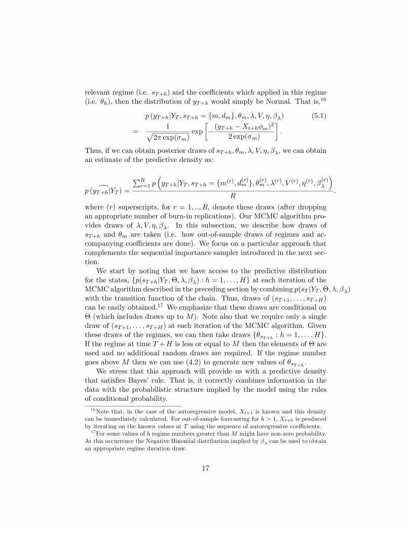
relevant regime (i.e. sT+h) and the coe¢ cients which applied in this regime(i.e. �h), then the distribution of yT+h would simply be Normal. That is,16

p (yT+hjYT ; sT+h = fm; dmg; �m; �; V; �; ��) (5.1)

=1p

2� exp(�m)exp

��(yT+h �Xt+h�m)

2

2 exp(�m)

�:

Thus, if we can obtain posterior draws of sT+h; �m; �; V; �; ��, we can obtainan estimate of the predictive density as:

dp (yT+hjYT ) =

PRr=1 p

�yT+hjYT ; sT+h = fm(r); d

(r)m g; �(r)m ; �(r); V (r); �(r); �(r)�

�R

:

where (r) superscripts, for r = 1; ::; R, denote these draws (after droppingan appropriate number of burn-in replications). Our MCMC algorithm pro-vides draws of �; V; �; ��. In this subsection, we describe how draws ofsT+h and �m are taken (i.e. how out-of-sample draws of regimes and ac-companying coe¢ cients are done). We focus on a particular approach thatcomplements the sequential importance sampler introduced in the next sec-tion.

We start by noting that we have access to the predictive distributionfor the states, fp(sT+hjYT ;�; �; ��) : h = 1; : : : ;Hg at each iteration of theMCMC algorithm described in the preceding section by combining p(sT jYT ;�; �; ��)with the transition function of the chain. Thus, draws of (sT+1; : : : ; sT+H)can be easily obtained.17 We emphasize that these draws are conditional on� (which includes draws up to M). Note also that we require only a singledraw of (sT+1; : : : ; sT+H) at each iteration of the MCMC algorithm. Giventhese draws of the regimes, we can then take draws f�sT+h : h = 1; : : : ;Hg.If the regime at time T +H is less or equal to M then the elements of � areused and no additional random draws are required. If the regime numbergoes above M then we can use (4.2) to generate new values of �sT+h .

We stress that this approach will provide us with a predictive densitythat satis�es Bayes�rule. That is, it correctly combines information in thedata with the probabilistic structure implied by the model using the rulesof conditional probability.16Note that, in the case of the autoregressive model, Xt+1 is known and this density

can be immediately calculated. For out-of-sample forecasting for h > 1; Xt+h is producedby iterating on the known values at T using the sequence of autoregressive coe¢ cients.17For some values of h regime numbers greater thanM might have non-zero probability.

At this occurrence the Negative Binomial distribution implied by �� can be used to obtainan appropriate regime duration draw.

17

5.2 Sequential Importance Sampling

Models such as ours are often used for real time forecasting. As new datacomes in, we want to update our forecasts. Of course, we could simplyre-run our MCMC algorithm with a data set augmented by this new dataand then calculate predictive densities as described in the previous section.However, in some cases, it is desirable to update forecasts without re-runningthe MCMC algorithm. In this section, we brie�y describe how sequentialimportance sampling methods [these are a popular type of particle �ltermethods, see, e.g., Doucet, Godsill and Andrieu (2000) or Liu and Chen(1998)] can be used with our model to achieve this goal.

Let zt = (�0t; St) denote the unobserved states and, for simplicity, sup-press conditioning arguments (all the p.d.f.s below are conditional on themodel parameters (�; V; �; ��)). The sequential importance sampler (SIS),is designed for models (such as ours) which can be written in terms of p (ytjzt)and p (ztjzt�1). Based on a sample of size T , posterior and predictive featuresdepend upon p (ZT jYT ) which can be obtained using our MCMC algorithmwhere Zi = (z1; : : : ; zi)

0. Now suppose a (T + 1)st observation becomes avail-able and, thus, posterior and predictive features depend on p (ZT+1jYT+1)which, by Bayes�rule, can be written as:

p (ZT+1jYT+1) = p (ZT jYT )p (yT+1jzT+1) p (zT+1jzT )

p (yT+1jYT ):

Since p (ZT jYT ) and p (yT+1jYT ) are impossible to directly evaluate simula-tion methods are required. The likelihood, p (yT+1jzT+1), is evaluated using(5.1).

We can, of course, use the MCMC algorithm described above to evaluateproperties of p (ZT+1jYT+1). However, an alternative is to use importancesampling. If we take an importance function of the form:

� (zT+1jZT ; YT+1) ;

then the importance sampling weights become:

wT+1 =p (ZT jYT ) p (yT+1jzT+1) p (zT+1jzT )

� (zT+1jZT ; YT+1):

If a (T + 2)nd observation becomes available and, hence, posterior and pre-dictive features depend on p (ZT+2jYT+2) which can also be handled usingimportance sampling. But note that the importance sampling weights nowbecome:

18

wT+2 = wT+1p (yT+2jzT+2) p (zT+2jzT+1)

� (zT+2jZT+1; YT+2):

In other words, we can recursively update the importance sampling weightsrather than evaluating them anew, reducing computational e¤ort. In gen-eral, importance sampling weights for T + h, are given by:

wT+h = wT+h�1p (yT+hjzT+h) p (zT+hjzT+h�1)

� (zT+hjZT+h�1; YT+h):

Computationally, such an approach can be very e¢ cient. That is, insteadof running a (computationally) demanding posterior simulation algorithmh+1 times (i.e. using data through period T + i for i = 0; 1; ::; h), the mainposterior simulation algorithm is run only once, and then SIS allows for thefast and e¢ cient updating as new information arises.

To be precise, if we begin using our MCMC algorithm for data throughperiod T , we obtain r = 1; ::; R draws. These can be interpreted as impor-tance sampling draws, each with an equal weight of 1

R . In period T + h,

using SIS we have R draws, each with weights w(r)T+h. As with any impor-tance sampler, posterior properties of any feature of interest can be found bytaking a weighted average of drawn features of interest using the normalizedweights:

ew(r)T+h = w(r)T+hPR

r=1w(r)T+h

:

Furthermore, the predictive likelihood18 for H observations can estimatedfrom the SIS output as:

dp(yT+1; ::; yT+H jYT ) =PRr=1w

(r)T+H

R:

The predictive likelihood for a single observation can be estimated using:

dp(yT+hjYT ) =RXr=1

p(yT+hjYT ; z(r)T+h�1; �(r); V (r); �(r); �

(r)� ) ew(r)T+h�1:

18As Poirier (1995), Chapter 8 discusses there is a lot of controversy in the frequen-tist literature about the meaning of predictive likelihood. In our Bayesian context theinterpretation is clear: it is the predictive distribution evaluated at the observed value foryT+h. Equivalently, it can be interpreted as a marginal likelihood, treating the posteriorat time T as a prior.

19

In theory, SIS could be used to draw the states for all time periods (i.e.we could set T = 0 in the preceding equations and simply have h indextime). However, all sequential importance sampling algorithms have theproperty that the variance of the importance sampling weights increase overtime (i.e. the algorithm becomes less e¢ cient as h increases). If the varianceof the importance sampling weights becomes too large, then the importancesampling estimates become dominated by only a few of the draws. Onesimple measure of the e¤ective number of draws is

bReffT+h = R1R

PRr=1(w

(r)T+h)

2

There are numerous methods [ see, e.g., Doucet, Godsill and Andrieu (2000)or Liu and Chen (1998)] which attempt to minimize this problem by usinga resampling technique when this e¤ective number of draws moves below athreshold. In our case, we have the advantage that if the e¤ective numberof draws falls below the threshold value we can always switch back to ouroriginal MCMC algorithm.

An obvious choice for the importance function in our case is our hierar-chical prior evaluated at the parameters values after observing the �rst Tobservations:

� (zT+hjZT+h�1; YT+h�1) = p (zT+hjzT+h�1; �; V; �; ��) :

To simulate from this importance function we use the same approach asdescribed for producing the predictive distributions.

5.3 Computation Issues in Context

Computation issues are important in the change-point literature. Unlessthe number of change-points is very small, the computational burden canbe quite demanding. Bayesian approaches, such as ours and Chib (1998),which adopt a hierarchical prior for the change-points, will have a muchlower computational burden than those which involve evaluating something(e.g. a likelihood or a posterior) at every possible set of change-points.Our MCMC approach largely draws on standard algorithms and, hence,programming costs are not large. Our approach will involve a computationalburden greater than Chib (1998) since our transition probabilities dependon the duration spent in each regime (see equation 3.3 and surroundingdiscussion). However, in both Chib (1998) and our model, the durations donot enter the likelihood (i.e. p (ytjYt�1; st = m) = p (ytjYt�1; �m) does not

20

depend on the duration of the regime), so the added computational burdenonly enters through draws of the states. With a modern personal computer,the computational burden of our approach is still trivial for data sets of thelength typically used by macroeconomists.19 Furthermore, methods suchas sequential importance sampling can be used to lessen the computationalburden in real time forecasting exercises. In our model the ability to usethe sequential importance sampling produces a tremendous reduction in netcomputation because most of the draws required are produced during theMCMC algorithm and just need to be stored.

The approach of Pesaran, Pettenuzzo and Timmerman (2006) sharesmany of the computational advantages of Chib (1998). However, some ofthe bene�ts of assuming a constant transition probability within a regime(except at the end of the sample), are lost in their forecasting exercise sincetheir assumed (out-of-sample) hierarchy is not conditionally conjugate andthe sequential importance sampling approach is not available due to theirimposition of a �xed number of change-points in sample. This contrasts toour hierarchy, which is conditionally conjugate.

In contrast to our approach, the in�uential non-Bayesian approach ofBai and Perron (1998) is less computationally burdensome. Bai and Perronstart from the observation that there are T (T+1)=2 ways of partitioning thesample. This is true in our approach as well, since we allow for any numberof breaks in sample. Bai and Perron then show how an e¢ cient dynamicprogramming method can be used to �nd the global least squares minimizerin the special case of all parameters in a linear conditional mean changingat each change-point with no restrictions on the coe¢ cients changes. Inthis special case they require only O(T 2) computations to �nd the leastsquares minimizer. Of course, without restrictions on the time betweenchange-points the minimum is achieved with a perfect �t. To get aroundthis issue, the minimizer is found by imposing additional restrictions on theminimum time between change-points. Inference is then performed by usinginsights from the asymptotic distribution. Note that this implies that adi¤erent partition of the data with the same number of change-points but aslightly higher value for the least squares minimand receives no weight in theinference. A strength of the Bayesian approach is that it puts weight on this

19A recent paper by Giordani and Kohn (2006) develops computationally e¢ cient meth-ods for the model of Chib (1998) and a simple version of our model. The authors showhow, in either of these models, break dates can be drawn in O(T ) operations by integrat-ing out the states analytically. It is probable that these methods can be extended for thegeneral version of our model and, thus, computation will be very e¢ cient indeed. Theworking paper version of our paper has further discussion on these points.

21

di¤erent partition. This would be particularly important for forecasting. Inan earlier working paper version, we discussed how a frequentist could usea hierarchical approach to obtain information on the probability of change-points at the global minimizer for the regime coe¢ cients found using Baiand Perron�s algorithm

Relative to the approach of Bai and Perron (1998, 2003), we would havethe same O(T 2) computational burden if we had assumed the standard con-stant transition probability matrix (and, we note this holds for a much widerclass of models than Bai and Perron). As we have seen, many Bayesian ap-proaches adopt this constant transition probability matrix, assuming a �xednumber of regimes occur in-sample. Our model is somewhat more compu-tationally demanding than this. However, a simpli�ed version of our modelwith a constant transition matrix would not be more computationally de-manding. Note that such a version of our model would allow for an unknownnumber of regimes in sample. In the case where the transition probabilitywas the same across regimes, the sequential importance sampler would beavailable and the net computational di¤erence for real time updating wouldfavor our method in most cases.

6 Application to US In�ation and Output

In economics, many applications of change-point modeling have been to thedecline in volatility of US real activity and changes in the persistence ofthe in�ation process. With regards to GDP growth, Kim, Nelson and Piger(2003), using the methods of Chib (1998) (assuming a single change-point),investigate breaks in various measures of aggregate activity. For most ofthe measures they consider, the likelihood of a break is overwhelming andBayesian and frequentist analyses produce very similar results.20 On theother hand, Stock and Watson (2002) present evidence from a stochasticvolatility model that the decline in variance might have been more gradual,a thesis �rst forward by Blanchard and Simon (2001).

Clark (2003) discusses the evidence on time variation in persistence inin�ation. Cogley and Sargent (2001, 2005) present evidence of time variation

20Since such papers consider only a single break, it is relatively easy to evaluate all thepossible break points. Kim, Nelson and Piger (2003) assume that the conditional meanparameters remain constant across the break and the only change is in the innovationvariance. If one allowed both the conditional mean and variance to break and assumed anexchangeable Normal- Gamma prior then the model can be evaluated analytically. Thiswas the approach followed in Koop and Potter (2001) and it has the advantage that onecan also integrate out over lag length in a trivial fashion.

22

in the in�ation process both in the conditional mean and conditional varianceof a smooth type. Stock (2001) �nds little evidence for variation in theconditional mean of in�ation using classical methods and Primiceri (2005)�nds some evidence for variation in the conditional variance but little in theconditional mean.

Accordingly, in our empirical work we investigate the performance of ourmodel using quarterly US GDP growth and the in�ation rate as measured bythe PCE de�ator (both expressed as an annual rates) from 1947Q2 through2005Q4. With both variables we include an intercept and two lags of thedependent variable as explanatory variables. We treat these �rst two lags asinitial conditions and, hence, our data e¤ectively runs from 1947Q4 through2005Q4.

In addition to our Poisson hierarchical model for durations we alsopresent results for standard TVP with stochastic volatility [see Stock andWatson 2002] and one-break models estimated using Bayesian methods.Both of these can be interpreted as restricted versions of our model. TheTVP model imposes the restrictions that the duration of each regime is one(i.e. st = t for all t). The one break model imposes the restriction thatthere are exactly two regimes with st = 1 for t � � and st = 2 for t > �(and the coe¢ cients are completely unrestricted across regimes with a �atprior on the coe¢ cients and error variances).21

The appendix describes our selection of the prior hyperparameters ��,�1,�2,��,��,V Vand �V and comparable prior hyperparameters for the TVP model. Herewe note only that we make weakly informative choices for these. In the ap-pendix we carry out a prior sensitivity analysis. The researcher interested inmore objective prior elicitation could work with a prior based on a trainingsample.

6.1 Estimation Results

Figure 1 presents information relating to the TVP for GDP growth. Theposterior means of the coe¢ cients (i.e. �t for t = 1; ::; T ) are given in Figure1a and the volatilities (i.e. exp(�t=2) for t = 1; : : : ; T ) in Figure 1b. Figure2 presents similar information from the one-break model.

Consider �rst results from the standard TVP and one break models forreal GDP growth. The most interesting �ndings for this variable relate tothe volatility. Both models indicate that volatility is decreasing substan-

21 In this one break model, we restrict the prior for the change-points such that thechange-point cannot occur in the �rst or last 5% of the sample.

23

tially over time, with a particularly dramatic drop occurring around 1984.22

However, with the TVP model this decline is much more smooth and non-monotonic than with the one break model. The question arises as to whetherthe true behavior of volatility is as suggested by the TVP model or the onebreak model. Of course, one can use statistical testing methods which com-pare these alternatives. However, an advantage of our model is that it neststhese alternatives. We can estimate what the appropriate pattern of changeis and see whether it is the TVP or the one break model �or something inbetween.

Our �ndings relating to volatility of GDP growth are not surprising givenprevious results starting with McConnell and Perez (2000). There is someevidence from the TVP model that volatility started to decline in the 1950sbut this decline was reversed starting in the late 1960s. The single breakmodel (by construction) does not show any evidence of this. The posterior ofthe breakpoint (not presented here), is quite tight and indicates the singlebreak to be at or very near to 1984. With regards to the autoregressivecoe¢ cients, with both models the posterior means suggest that little changehas taken place. However, posterior standard deviations (not presented) arequite large indicating a high degree of uncertainty. In the literature [e.g.Stock and Watson (2002)] these �ndings have been interpreted as implyingthat there has been no change in the conditional mean parameters.

In light of this approximate constancy of the coe¢ cients (and to illustrateour methods in an interesting special case), we estimate our model withvariation only in the volatilities and not in the coe¢ cients. That is, the�rst equation in (4.2) is degenerate (or, equivalently, V = 0K�K). Figure3 plots features of the resulting posterior for the most interesting feature:volatility.23 This �gure is smoother but otherwise similar to the comparableTVP result in Figure 1b, but di¤ers quite substantially from the one breakmodel result. With our model, the number of regimes in-sample can beestimated. Its posterior mean is 45:35 (with posterior standard deviationof 12:70). This lies somewhere between the one break and TVP models(where the latter, by de�nition, will have T = 233 regimes). Thus, we are�nding evidence that a model between the one break and TVP models ismost sensible (although the TVP model is more sensible than the one break

22Note that, in the one break model, the posterior means of the coe¢ cients and volatil-ities, conditional on a particular change-point, will behave like step functions. However,when we present unconditional results, which average over possible change-points, thisstep function pattern is lost as can be seen in the �gures.23The prior sensitivity analysis done in the appendix presents more posterior results for

our model.

24

model). We stress that we have found such evidence in the context of amodel which could have allowed for very few breaks.

Let us now turn to in�ation. Given �ndings by other authors and aninterest in the persistence of in�ation, we use the unrestricted version of ourmodel and allow the AR coe¢ cients to change across regimes. Figures 4, 5and 6 present results from the TVP, one break and our models, respectively.Figure 4a, containing the sum of the two autoregressive parameters from theTVP model, shows an increasing tendency in the persistence of in�ation upto the late 1970s followed by a decreasing tendency. The fact that the levelof in�ation increased throughout the 1970s and early 1980s before decliningin the 1990s is picked up partly through the pattern in the intercept. Thevolatility of in�ation shows a similar pattern, with a noted increase in the1970s and early 1980s. These sensible results are found by both the TVPmodel and our model and are consistent with evidence presented in Cogleyand Sargent (2001), although at odds with some of the evidence presented inPrimiceri (2005). But it is worth noting that our model smooths out someof the erratic patterns produced by the TVP model. The single break modelindicates quite di¤erent patterns (see Figure 5). It wants to put the singlebreak near the beginning of the sample, totally missing any changes in thelevel, persistence or volatility of in�ation in the 1970s and early 1980s. Onecould force the break later by adopting a prior that the change-point is laterin the sample.

When comparing results from the TVP and one break model to ours, asa general rule we are �nding our model supports many change-points ratherthan a small number and thus the movements of the conditional mean andvariance parameters are closer to the TVP model. We take this as evidencethat our methods are successfully capturing the properties of a reasonabledata generating process, but without making the assumption of a breakevery period as with the TVP model. That is, we are letting the data tellus what key properties of the data are, rather than assuming them. Ourempirical results also show the problems of working with models with a smallnumber of breaks when, in reality, the evolution of parameters is much moregradual.

6.2 Predictive Exercise

The previous section focusses on estimation for our model, the TVP modeland a one break model. In order to compare these di¤erent models, wecould calculate marginal likelihoods in order to construct Bayes�factors orposterior odds ratios using standard methods. For instance, the methods

25

of Chib (1995), Chib and Jeliazkov (2001) or Gelfand and Dey (1994) canbe used to estimate the marginal likelihood in change-point models. Moresimply, information criteria such as the Schwarz criteria can be used toapproximate marginal likelihoods. However, in these models (which are veryparameter rich) marginal likelihoods can be sensitive to priors. Accordingly,we prefer to compare models using predictive criteria such as the predictivelikelihood discussed in Sections 5.1 and 5.2. As discussed in Section 5.2,these can easily be calculated using sequential importance sampling.

Table 1 presents predictive likelihoods for a period of two years at theend of our sample. That is, we use data through period 2003Q4 to calculatepredictive distributions for each quarter through 2005Q4 and then evaluatethe predictive at the observed outcome. It can be seen that, in terms ofoverall forecast performance over these 8 observations, our model does sub-stantially outperform the one break model and (less substantially) the TVPmodel.

Table 1: Joint Predictive Likelihoods for 2004/2005Our Model TVP One Break

GDP Growth 9.77�10�7 6.06�10�7 4.93�10�7In�ation 3.69�10�6 3.31�10�6 1.75�10�6

Table 1 presents results relating to joint performance over two years. Ina real time forecasting exercise, one might also be interested in forecastingperformance one quarter at a time (where each quarter new data is usedto update the predictive density). To illustrate how this can be done, wecarry out a pseudo real-time forecasting exercise for 2004 and 2005. Thatis, beginning in 2003Q4 we construct the predictive distribution for 2004Q1,then use data through 2004Q1 to predict 2004Q2, etc.. A simple summaryof forecasting performance involves seeing where the actual outcome lies inthese one-period-ahead predictive distributions. In particular, we can calcu-late where the actual outcome lies in the predictive cumulative distributionfunction. Table 2 presents this information for our three models and twodata series. An informal examination of Table 2 suggests all three of ourmodels are predicting GDP growth fairly well. None of the outcomes are toofar out in the tails of the predictive distributions. This is unsurprising since2004-2005 were years of stable GDP growth with little evidence of structuralchange. More formal metrics of predictive performance can be developed bynoting that, if a model is correct and there is no parameter uncertainty,then probabilities such as those in Table 2 should be drawn from the Uni-form [0,1] distribution [see, e.g., Diebold, Gunther and Tay (1998)]. Using

26

the numbers in Table 2, the standard Chi-squared statistics for testing forUniformity [e.g., Wonnacott and Wonnacott (1990), pages 550-551] are 9.5,9.5 and 12.0 for our model, the TVP and the one break model, respectively.This provides some evidence that our model and the TVP are forecastingcomparably to one another and the one break model is doing slightly worse.Note that the frequentist 0.05 critical value is 16.9 so we cannot reject thehypothesis of Uniformity for any of our models.

For in�ation (which was somewhat more erratic in the 2004-2005 period),the Chi-squared statistics for testing Uniformity of the numbers in Table 2are 12.0, 9.5 and 17.0 for our model, the TVP and the one break model,respectively. Hence, for in�ation we are �nding the TVP model forecastsslightly better than the other models. Furthermore, the frequentist hypoth-esis that the one break model is correct can be rejected at the 5% level ofsigni�cance.

Table 2: Predictive Probability of Being Less than Actual OutcomeGDP growth In�ationOur Model TVP One Break Our Model TVP One Break

2004Q1 0.581 0.579 0.485 0.966 0.967 0.9422004Q2 0.525 0.456 0.582 0.935 0.935 0.7682004Q3 0.601 0.636 0.635 0.125 0.096 0.0352004Q4 0.514 0.499 0.535 0.732 0.711 0.7372005Q1 0.628 0.649 0.663 0.852 0.830 0.7812005Q2 0.533 0.510 0.557 0.503 0.471 0.4002005Q3 0.726 0.732 0.733 0.840 0.822 0.7602005Q4 0.186 0.179 0.225 0.805 0.755 0.653

7 Conclusions

In this paper we have developed a change-point model which nests a widerange of commonly-used models, including TVP models and those with asmall number of structural breaks. Our model satis�es the six criteria setout in the introduction. In particular, the maximum number of regimes inour model is not restricted and it has a �exible Poisson hierarchical priordistribution for the durations. Furthermore, we allow for information (bothabout durations and coe¢ cients) from previous regimes to a¤ect the currentregime. The latter feature is of particular importance for forecasting.

Bayesian methods for inference and prediction are developed and appliedto real GDP growth and in�ation series. We compare our methods to two

27

common models: a single-break model and a time varying parameter model.We �nd our methods to reliably recover key data features without makingthe restrictive assumptions underlying the other models.

8 References

Ang, A. and Bekaert, G., 2002, Regime switches in interest rates, Journalof Business and Economic Statistics, 20, 163-182.

Bai, J. and Perron, P., 1998, Estimating and testing linear models withmultiple structural changes, Econometrica, 66, 47-78.

Bai, J. and Perron, P., 2003, Computation and analysis of multiple struc-tural change models, Journal of Applied Econometrics 18, 1-22.

Barry, D. and Hartigan, J., 1993, A Bayesian analysis for change pointproblems, Journal of the American Statistical Association, 88, 309-319.

Bayarri, M., DeGroot, M. and Kadane, J., 1988, What is the likelihoodfunction? pp. 1-27 in Statistical Decision Theory and Related Topics IV,volume 1, edited by S. Gupta and J. Berger, New York: Springer-Verlag.

Blanchard, O. and Simon, J., 2001, The long and large decline in USoutput volatility, Brookings Papers on Economic Activity, 1, 135-174.

Bracqemond, C. and Gaudoin, O., 2003, A survey on discrete lifetimedistributions, International Journal of Reliability, Quality and Safety Engi-neering, 10, 69-98.

Carlin, B., Gelfand, A. and Smith, A.F.M., 1992, Hierarchical Bayesiananalysis of changepoint problems, Applied Statistics, 41, 389-405.

Carter, C. and Kohn R., 1994, On Gibbs sampling for state space models,Biometrika, 81, 541-553.

Cherno¤, H. and Zacks, S., 1964, Estimating the current mean of a Nor-mal distribution which is subject to changes in time, Annals of MathematicalStatistics, 35, 999-1018.

Chib, S., 1995, Marginal likelihood from the Gibbs Sampler, Journal ofthe American Statistical Association, 90, 1313-1321.

Chib, S., 1996, Calculating posterior distributions and modal estimatesin Markov mixture models, Journal of Econometrics, 75, 79-97.

Chib, S., 1998, Estimation and comparison of multiple change-pointmodels, Journal of Econometrics, 86, 221-241.

Chib, S. and Jeliazkov, I., 2001. Marginal likelihood from the Metropolis-Hastings output, Journal of the American Statistical Association, 96, 270-281.

28

Chopin, N. and Pelgrin, F., 2004, Bayesian inference and state numberdetermination for hidden Markov models: An application to the informationcontent of the yield curve about in�ation, Journal of Econometrics, 123,327-344.

Clark, T., 2003, Disaggregate evidence on the persistence of consumerprice in�ation, Federal Reserve Bank of Kansas City, Working Paper RP#03-11 available at http://www.kc.frb.org/publicat/reswkpap/PDF/RWP03-11.pdf

Clements, M. and Hendry, D., 1998, Forecasting Economic Time Series.(Cambridge University Press: Cambridge).

Clements, M. and Hendry, D., 1999, Forecasting Non-stationary Eco-nomic Time Series. (The MIT Press: Cambridge).

Cogley, T. and Sargent, T., 2001, Evolving post-World War II in�ationdynamics, NBER Macroeconomic Annual.

Cogley, T. and Sargent, T., 2005, Drifts and volatilities: monetary poli-cies and outcomes on Post WWII US, Review of Economic Dynamics, 8,262-302.

DeJong, P. and Shephard, N., 1995, The simulation smoother for timeseries models, Biometrika, 82, 339-350.

Diebold, F., Gunther, T. and Tay, A., 1998, Evaluating density forecastswith applications to �nancial risk management, International Economic Re-view, 39, 863-883.

Doucet, A., Godsill, S. and Andrieu, C., 2000, On sequential MonteCarlo sampling methods for Bayesian �ltering, Statistics and Computing,10, 197-208.

Durbin, J. and Koopman, S., 2002, A simple and e¢ cient simulationsmoother for state space time series analysis, Biometrika, 89, 603-616.

Elliott, G. and Muller, U., 2006, Optimally testing general breakingprocesses in linear time series models, Review of Economic Studies, forth-coming.

Fernandez, C., Osiewalski, J. and Steel, M.F.J., 1997, On the use ofpanel data in stochastic frontier models with improper priors, Journal ofEconometrics, 79, 169-193.

Gelfand, A. and Dey, D., 1994, Bayesian model choice: Asymptotics andexact calculations, Journal of the Royal Statistical Society Series B, 56, 501-514.

Giordani, P. and Kohn, R., 2006, E¢ cient Bayesian inference for multiplechange-point and mixture innovation model, manuscript.

Hamilton, J., 1994, Time Series Analysis. Princeton: Princeton Univer-sity Press.

29

Kim, C., Nelson, C. and Piger. J., 2003, The less volatile U.S. economy:A Bayesian investigation of timing, breadth, and potential explanations,working paper 2001-016C, The Federal Reserve Bank of St. Louis.

Kim, S., Shephard, N. and Chib, S., 1998, Stochastic volatility: likeli-hood inference and comparison with ARCH models, Review of EconomicStudies, 65, 361-93.

Koop, G. and Poirier, D., 2004, Empirical Bayesian inference in a non-parametric regression model, in State Space and Unobserved ComponentsModels Theory and Applications, edited by Andrew Harvey, Siem Jan Koop-man and Neil Shephard (Cambridge University Press: Cambridge).

Koop, G. and Potter, S., 2001, Are apparent �ndings of nonlinearity dueto structural instability in economic time series?, The Econometrics Journal4, 37-55.

Koop, G. and Potter, S., 2004, Prior elicitation in multiple change-pointmodels, working paper available at http://www.le.ac.uk/economics/gmk6/.

Liu, J. and Chen, R., 1998, Sequential Monte Carlo methods for dy-namic systems, Journal of the American Statistical Association, 93, 1032�1044.

Maheu, J. and Gordon, S., 2005, Learning, forecasting and structuralbreaks, manuscript available at http://www.chass.utoronto.ca/~jmaheu/mg.pdf.

McConnell, M. and Perez, G., 2000, Output �uctuations in the UnitedStates: What has changed since the early 1980s? American Economic Re-view 90 1464-76.

McCulloch, R. and Tsay, E., 1993, Bayesian inference and predictionfor mean and variance shifts in autoregressive time series, Journal of theAmerican Statistical Association, 88, 968-978.

Nyblom, J.1989, Testing for the constancy of parameters over time, Jour-nal of the American Statistical Association, 84, 223-230.

Pastor, L. and Stambaugh, R., 2001, The equity premium and structuralbreaks, Journal of Finance, 56, 1207-1239.

Pesaran, M.H., Pettenuzzo, D. and Timmerman, A., 2006, Forecastingtime series subject to multiple structural breaks, Review of Economic Stud-ies, forthcoming.

Poirier, D., 1995, Intermediate Statistics and Econometrics: A Compar-ative Approach. Cambridge: The MIT Press.

Primiceri, G., 2005, Time varying structural vector autoregressions andmonetary policy, Review of Economic Studies, 72, 821-852.

Stock, J., 2001, Comment on Cogley and Sargent, NBER MacroeconomicAnnual.

30

Stock, J. and Watson, M., 1996, Evidence on structural instability inmacroeconomic time series relations, Journal of Business and Economic Sta-tistics, 14, 11-30.

Stock J. and Watson M., 2002 Has the business cycle changed and why?NBER Macroeconomic Annual.

Wonnacott, T. and Wonnacott, W., 1990, Introductory Statistics forBusiness and Economics (Fourth edition). New York: John Wiley and Sons.

Appendix: Properties of the Prior and Prior Sensi-tivity Analysis

In the body of the text, we developed some theoretical properties of theprior. However, given its complexity, it is also instructive to examine itsimplications using prior simulation. Accordingly, in this appendix, we illus-trate some key properties of our prior for the hyperparameter values used inthe empirical work as well as carry out a prior sensitivity analysis. We useinformative priors. For highly parameterized models such as this, prior in-formation can be important. Indeed, results from the Bayesian state spaceliterature show how improper posteriors can result with improper priors[see, e.g. Koop and Poirier (2004) or Fernandez, Ley and Steel (1997)]. Onestrategy commonly-pursued in the related literature [see, e.g., Cogley andSargent (2001, 2005)] is to restrict coe¢ cients to lie in bounded intervals such(e.g. the stationary interval). This is possible with our approach. However,this causes substantial computational complexities (which are of particularrelevance in our model where many regimes can occur out-of-sample and re-�ect relatively little data information). Training sample priors can be usedby the researcher wishing to avoid subjective prior elicitation.

In this paper, we choose prior hyperparameter values which attach ap-preciable prior probability to a wide range of reasonable parameter values.To aid in interpretation, note that our data is measured as a percentage and,hence, changes in �m in the interval [�0:5; 0:5] are the limit of plausibility.For AR coe¢ cients, the range of plausible intervals is likely somewhat nar-rower than this. With regards to the durations, we want to allow for veryshort regimes (to approach the TVP model) as well as much longer regimes(to approach a model with few breaks). We choose values of the prior hy-perparameters, ��; �1; �2; ��; ��; V V and �V which exhibit such properties.

Figures A1 through A3 plot the prior for key features assuming �� =12; �

1= ��; �2 = ��; �� = 1:0; �� = 0:02; V V = 0:1IK and �V = 3K. Note

that, by construction, the priors for all our conditional mean coe¢ cients

31

are the same so we only plot the prior for the AR(1) coe¢ cient. FigureA1 plots the prior over durations and it can be seen that the prior weightis spread over a wide range, from durations of 1 through more than 50receiving appreciable prior weight. Figures A2 and A3 plot prior standarddeviations for the state equation innovations (see 4.2). It can be seen thatthese are di¤use enough to accommodate anything from the very small shiftsconsistent with a TVP model through much bigger shifts of a small breakmodel.

For the TVP model, we make the same prior hyperparameter choices(where applicable). The prior for the one break model has already beendescribed in the text.

In a sense, by presenting results for the TVP and one break models, wehave already carried out a prior sensitivity analysis. That is, the TVP modelcan be considered as an extreme case where we use a dogmatic prior whichimposes a break every time period and the one break model a dogmaticprior which imposes a precise number of breaks. However, in this appendixwe provide some additional evidence on prior sensitivity with regards to themost important feature of our model: the prior on regime duration. In thisregard, the prior for � is of most importance and it is characterized by twoparameters, �

1and �

2. In the empirical results section, we have set �

1=

�2= 12, values which yield the prior over durations in Figure A.1. Equation

3.5 and the discussion following it describes the prior. For present purposes,perhaps the most important things are to note that the prior mean of dm is

1 + ��

�2

�1� 1

!;

if �1> 1 and the properties of the Gamma distribution can be used to

understand the other aspect of the prior. We consider an extremely widerange of prior hyperparameter values by allowing for �

1= 1; 12; 100 and

�2= 1; 12; 100. Table A.1 relates to GDP growth and presents the posterior

properties of a key feature in our model: the number of in-sample regimes.Note that our base prior, used in the empirical work, provides an estimate of45:35 regimes in-sample (with posterior standard deviation of 12:70). This isbetween the T = 233 regimes implied by the TVP model and the 2 regimesimplied by the one break model. As we tighten the prior towards havingshort durations (i.e. towards the TVP model), by increasing �

1or decreasing

�2, the number of regimes in sample does indeed increase (although this

has relatively little e¤ect on �gures such as Figure 3 or on the predictivefeatures). Tightening the prior in the direction of the one-break model (by

32

decreasing �1or increasing �

2) the number of regimes in sample does indeed

decrease, but never to fewer than 12. That is, even if we set prior where themean duration of a regime is very close to one, there is enough informationin the data to pull the posterior in the direction of many regime changes.

Table A.1: Prior Sensitivity AnalysisFor GDP GrowthPosterior Mean of # Regimes

�2= 1 �

2= 12 �

2= 100

�1= 1 73:32 12:48 12:15

�1= 12 74:16 45:35 12:17

�1= 100 78:29 76:23 17:38

Table A.2 repeats the analysis for in�ation. Similar patterns appears.Note that, as expected, the in�ation data is closer to coming from a TVPmodel than the GDP growth data. With our base prior, the number of in-sample regimes is estimated to be 124:00 (with posterior standard deviationof 32:64). Very large changes in the prior o¤er little change in this story.Even when the prior pulls strongly towards model with few breaks, theposterior still indicates very many breaks in-sample (i.e. the posterior meannumber of regimes is at least 86:96). When the prior is shifted towards theTVP model, the number of in-sample breaks increases slightly, but the basic�ndings of our model are una¤ected.

Table A.2: Prior Sensitivity AnalysisFor In�ationPosterior Mean of # Regimes(Post. St. Dev. in parentheses)

�2= 1 �

2= 12 �

2= 100

�1= 1 189:25 90:32 86:96

�1= 12 189:80 124:00 87:96

�1= 100 190:62 186:85 88:92

33

34

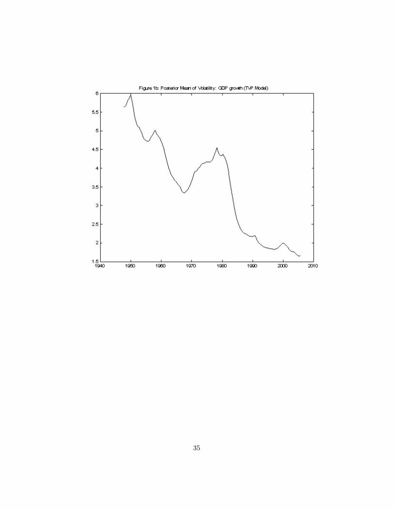
35

36

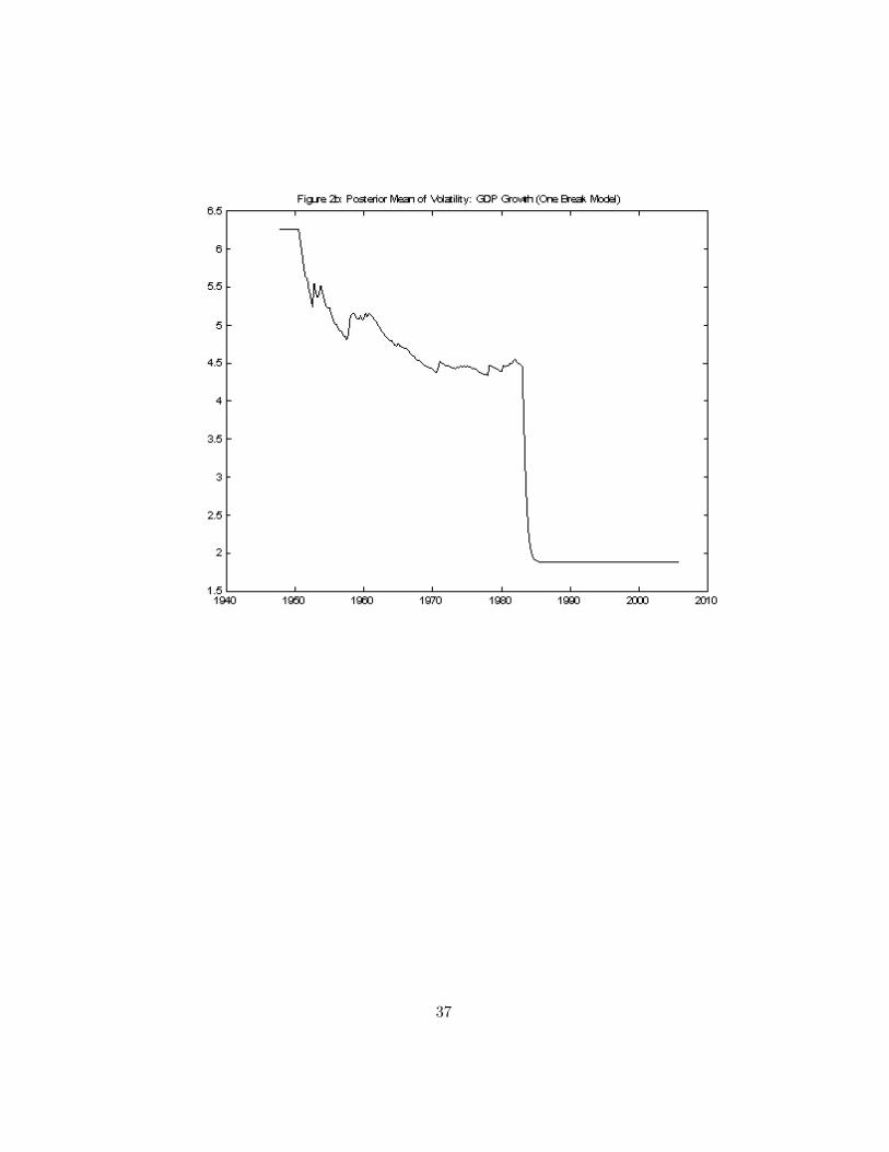
37

38

39

40

41

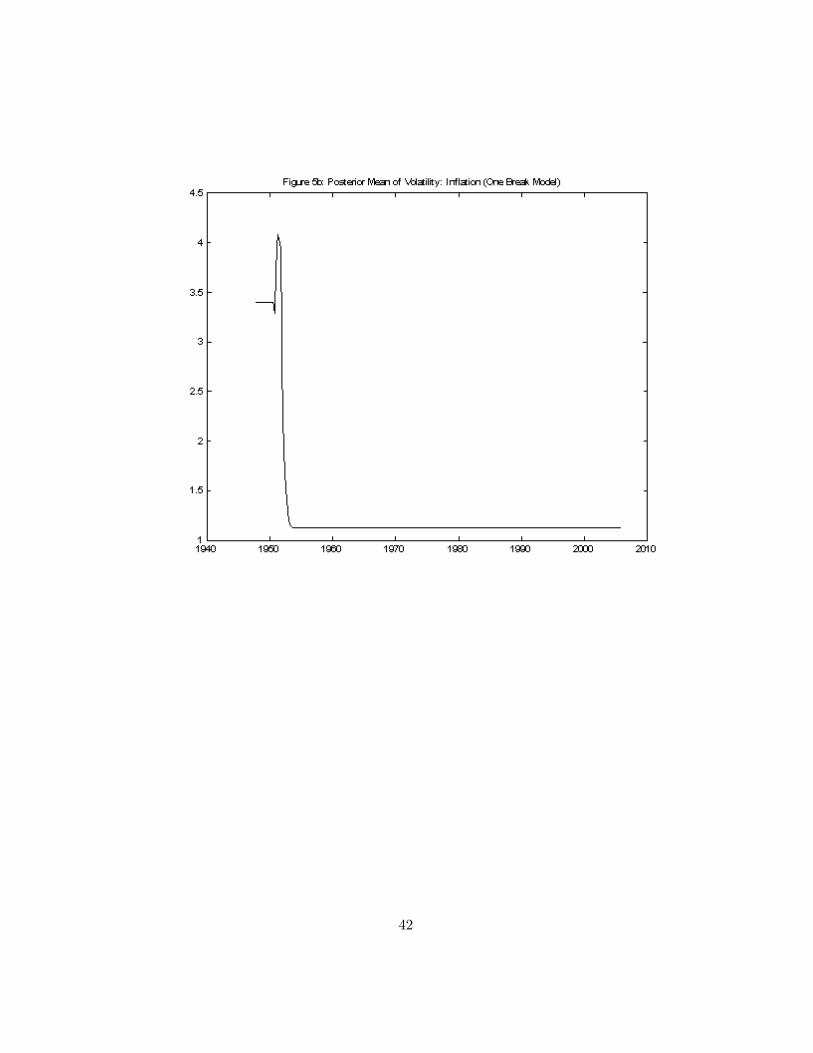
42

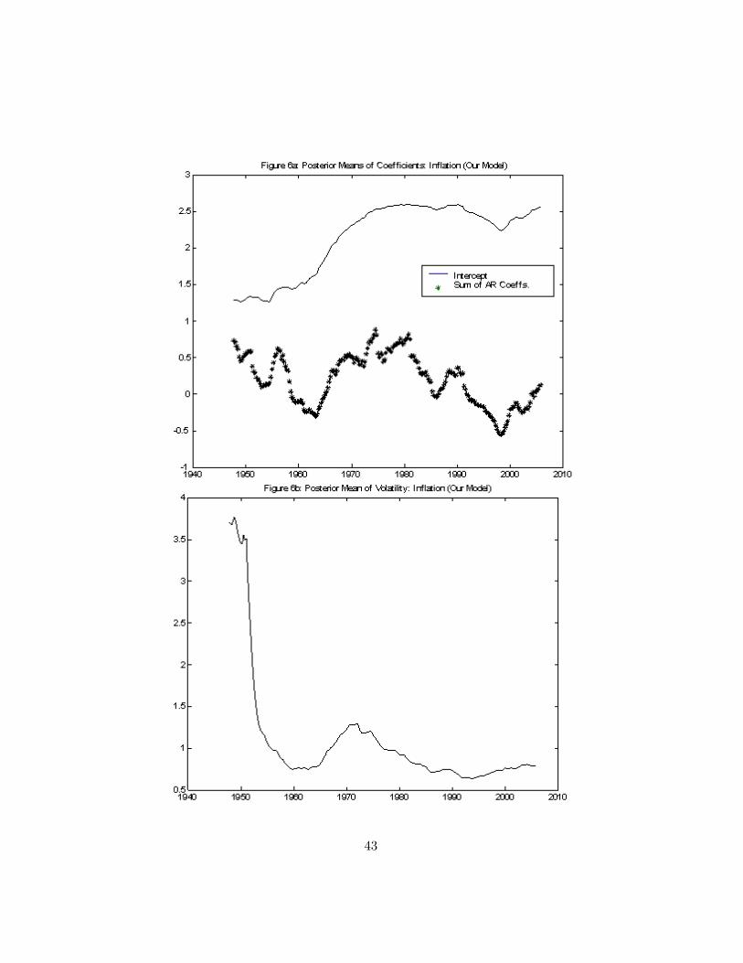
43

44

45