Estimating Wind Power Potential And Its Variabilities Over ...
39
Estimating Wind Power Potential And Its Variabilities Over Europe PÉTER KISS, IMRE M. JÁNOSI, LÁSZLÓ VARGA, FLAVIO BONO, EUGENIO GUTIERREZ DEPARTMENT OF PHYSICS OF COMPLEX SYSTEMS, LORÁND EÖTVÖS UNIVERSITY, BUDAPEST; COLLEGIUM BUDAPEST, BUDAPEST; E.ON HUNGÁRIA LTD, BUDAPEST; JOINT RESEARCH CENTRE, ISPRA P. Kiss e-mail: [email protected] I. M. Jánosi web: http://lecso.elte.hu
Transcript of Estimating Wind Power Potential And Its Variabilities Over ...
Estimating Wind Power Potential And Its Variabilities Over Europe
PÉTER KISS, IMRE M. JÁNOSI, LÁSZLÓ VARGA, FLAVIO BONO, EUGENIO GUTIERREZ
DEPARTMENT OF PHYSICS OF COMPLEX SYSTEMS, LORÁND EÖTVÖS UNIVERSITY, BUDAPEST;
COLLEGIUM BUDAPEST, BUDAPEST;E.ON HUNGÁRIA LTD, BUDAPEST;JOINT RESEARCH CENTRE, ISPRA
P. Kiss e-mail: [email protected]. M. Jánosi web: http://lecso.elte.hu
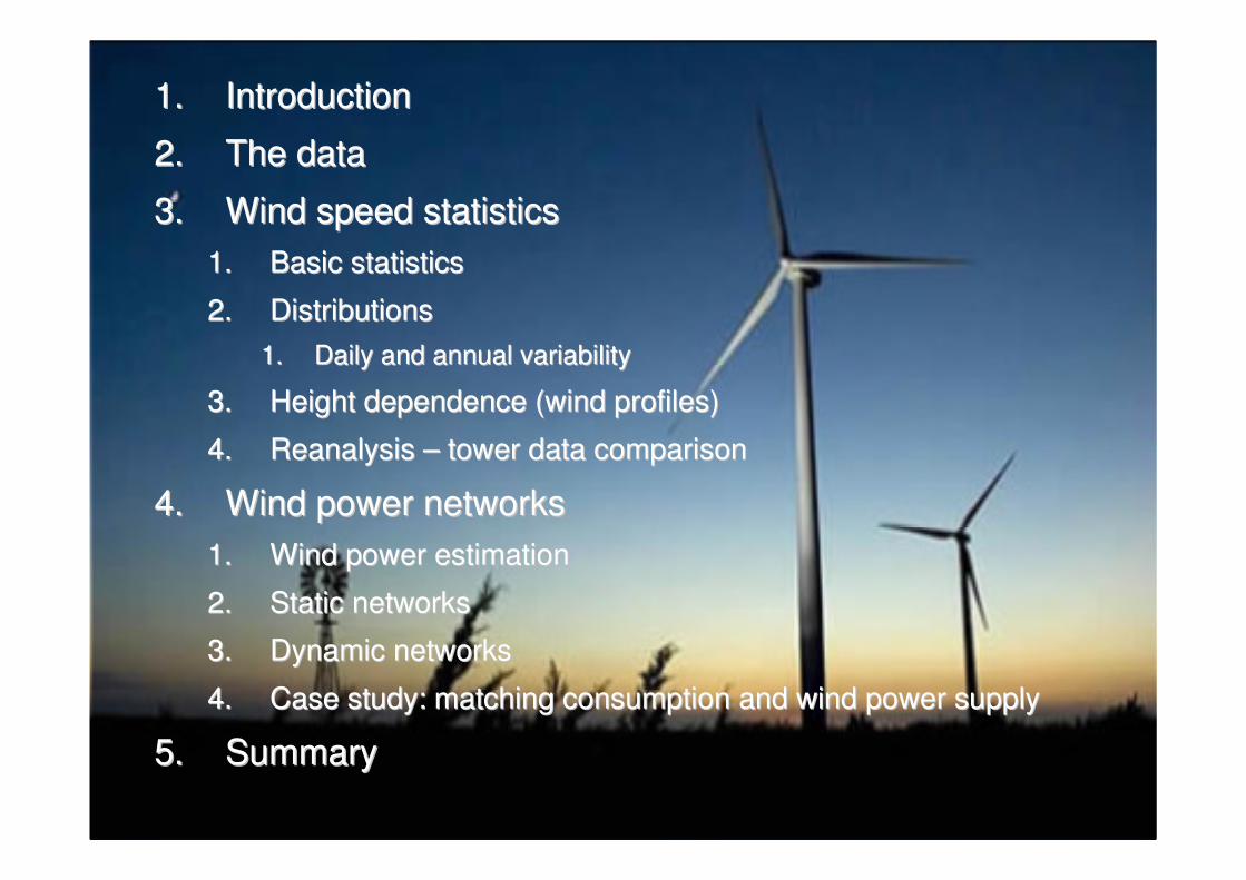
1.1. IntroductionIntroduction
2.2. The dataThe data
3.3. Wind speed statisticsWind speed statistics1.1. Basic statisticsBasic statistics
2.2. DistributionsDistributions
1.1. Daily and annual variabilityDaily and annual variability
3.3. Height dependence (wind profiles)Height dependence (wind profiles)
4.4. Reanalysis Reanalysis –– tower data comparisontower data comparison
4.4. Wind power networksWind power networks1.1. Wind power estimationWind power estimation
2.2. Static networksStatic networks
3.3. Dynamic networksDynamic networks
4.4. Case study: matching consumption and wind power supplyCase study: matching consumption and wind power supply
5.5. SummarySummary

1. Introduction – Global power consumption
Solar radiation: 1520 EWh (outside the atmosphere) (174 PW average)
2005 data:Global energy consumption:
140 PWh (16 TW average)
~0.01 % of the solar radiation !
Electricity out of this:16.6 PWh (1.9 TW average)
E (exa) 1018
P (peta) 1015
T (tera) 1012 Source: Wikipedia, 2006 data
Global energy usage

1. Introduction – Global wind power – present state
Global installed wind power nameplate capacity: 121.2 GW (2008)
Europe: 64.9 GW (2008)
1.5 % of electricity generated
by wind farms (global, 2008)
Source: Wikipedia
Source: World Wind Energy Associationhttp://www.wwindea.org/
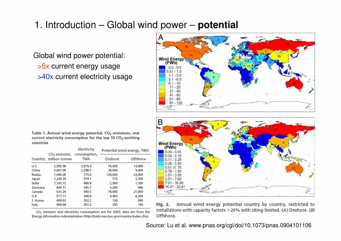
1. Introduction – Global wind power – potential
Global wind power potential:
>5x current energy usage>40x current electricity usage
Source: Lu et al. www.pnas.org/cgi/doi/10.1073/pnas.0904101106
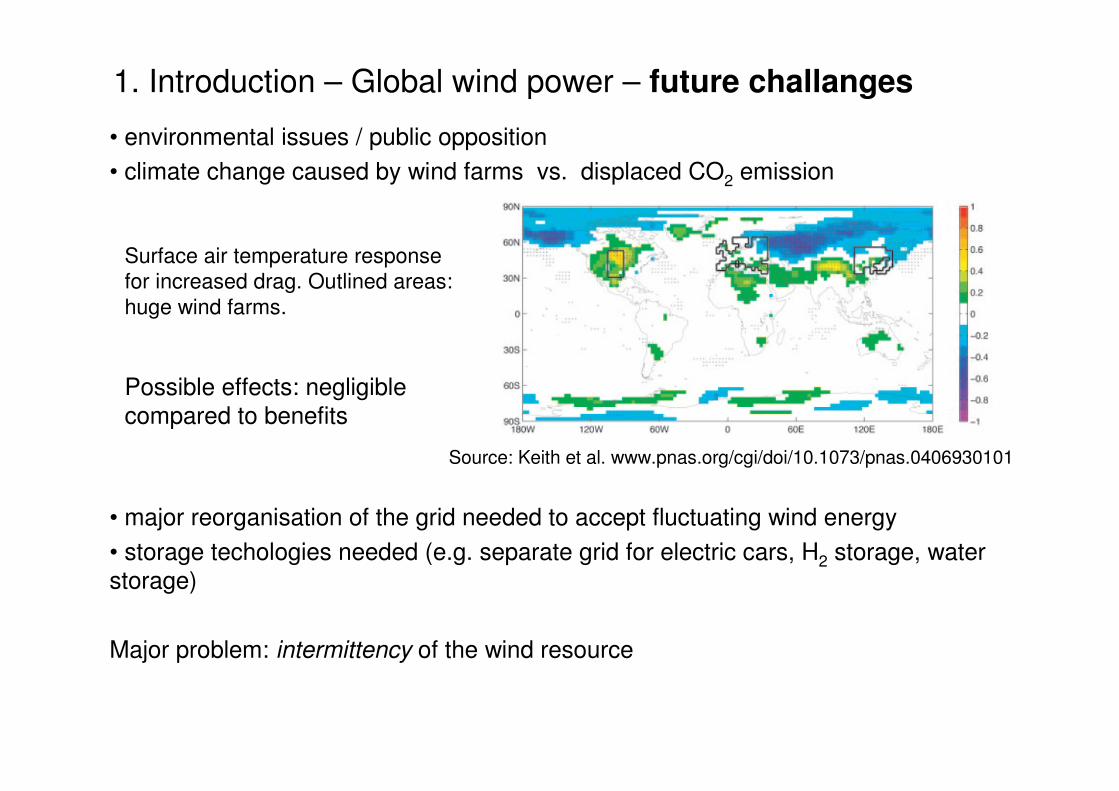
1. Introduction – Global wind power – future challanges
• environmental issues / public opposition• climate change caused by wind farms vs. displaced CO2 emission
• major reorganisation of the grid needed to accept fluctuating wind energy
• storage techologies needed (e.g. separate grid for electric cars, H2 storage, water storage)
Major problem: intermittency of the wind resource
Source: Keith et al. www.pnas.org/cgi/doi/10.1073/pnas.0406930101
Surface air temperature response for increased drag. Outlined areas: huge wind farms.
Possible effects: negligible compared to benefits
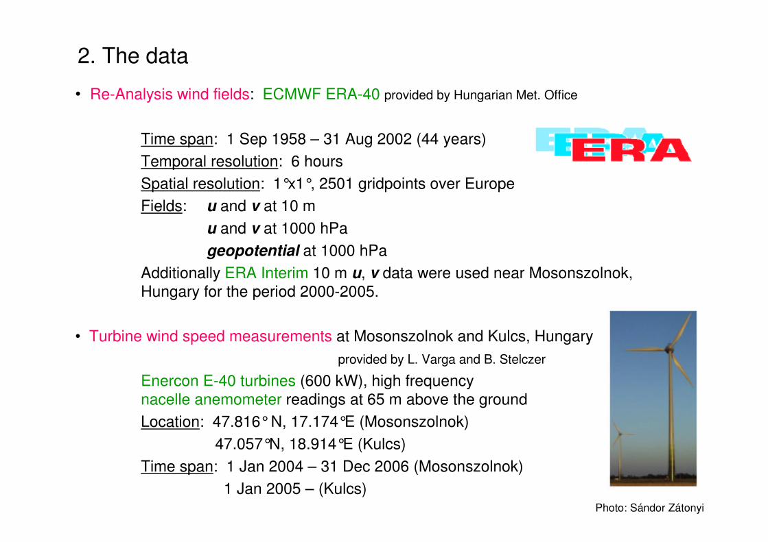
2. The data
• Re-Analysis wind fields: ECMWF ERA-40 provided by Hungarian Met. Office
Time span: 1 Sep 1958 – 31 Aug 2002 (44 years)Temporal resolution: 6 hoursSpatial resolution: 1°x1°, 2501 gridpoints over EuropeFields: u and v at 10 m
u and v at 1000 hPageopotential at 1000 hPa
Additionally ERA Interim 10 m u, v data were used near Mosonszolnok, Hungary for the period 2000-2005.
• Turbine wind speed measurements at Mosonszolnok and Kulcs, Hungaryprovided by L. Varga and B. Stelczer
Enercon E-40 turbines (600 kW), high frequency nacelle anemometer readings at 65 m above the groundLocation: 47.816° N, 17.174°E (Mosonszolnok)
47.057°N, 18.914°E (Kulcs)Time span: 1 Jan 2004 – 31 Dec 2006 (Mosonszolnok)
1 Jan 2005 – (Kulcs)Photo: Sándor Zátonyi
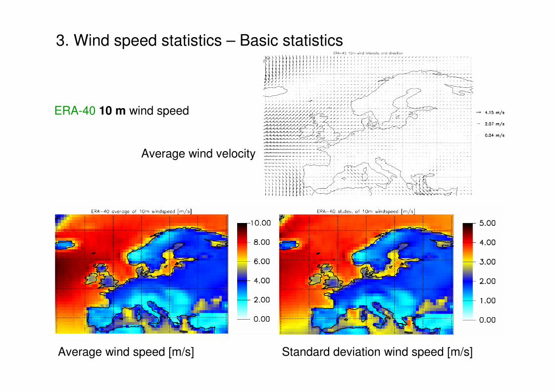
3. Wind speed statistics – Basic statistics
ERA-40 10 m wind speed
Average wind velocity
Average wind speed [m/s] Standard deviation wind speed [m/s]

3. Wind speed statistics – Basic statistics
Animation showing ERA-40 wind filelds at 10 m above the surface
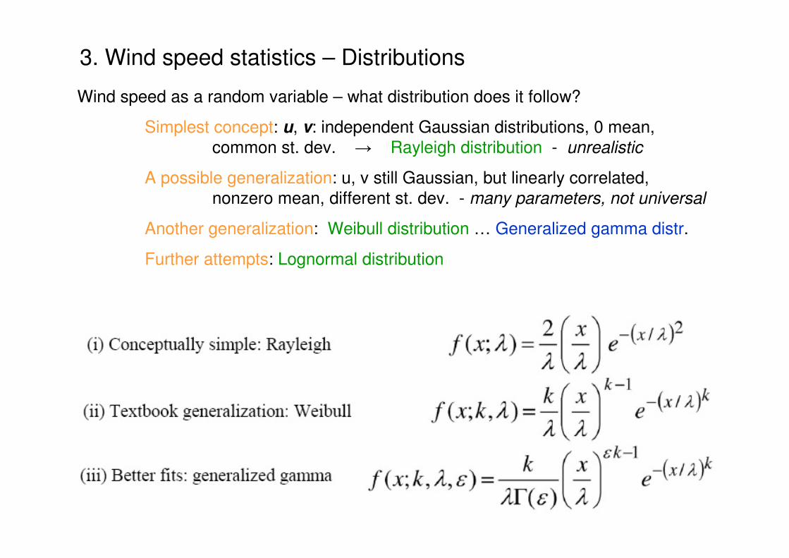
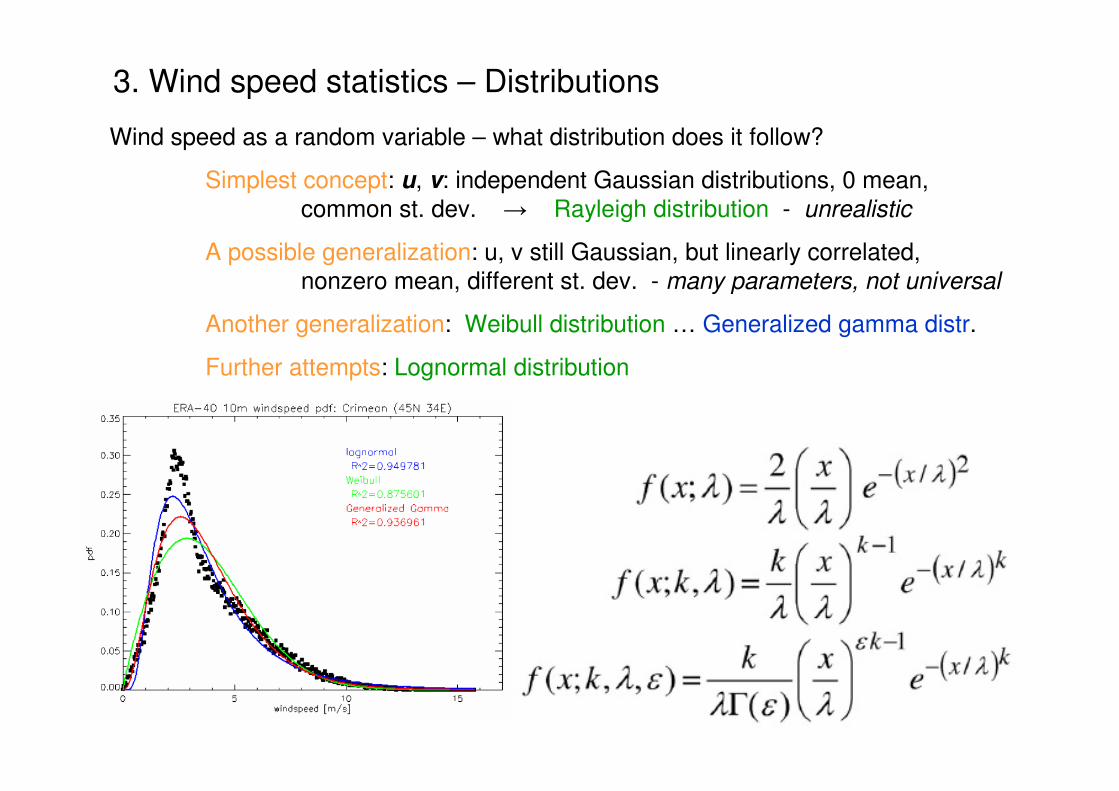
3. Wind speed statistics – Distributions
Wind speed as a random variable – what distribution does it follow?
Simplest concept: u, v: independent Gaussian distributions, 0 mean, common st. dev. → Rayleigh distribution - unrealistic
A possible generalization: u, v still Gaussian, but linearly correlated, nonzero mean, different st. dev. - many parameters, not universal
Another generalization: Weibull distribution … Generalized gamma distr.
Further attempts: Lognormal distribution

3. Wind speed statistics – Distributions
Goodness of fit of different distributions:
100 (1-R2)
unexplained percentage variance
Best:
Generalized gamma distribution
Weibull distribution
Joint Gaussian distribution Generalized gamma distribution

3. Wind speed statistics – Distributions
The Generalized gamma (GG) fit
Left tail shape parameter
Right tail shape parameter
Left tail shape parameter
Rig
ht ta
il sh
ape
para
met
er

3. Wind speed statistics – Daily and annual varability
FFT power spectra: total power = 1
Daily power
Yearly power
By removing daily and yearly cycles (u
and v) from wind speed records, the GG
fit substantially improves.
Wind speed pdf at the Crimean peninsula

3. Wind speed statistics – Height dependence
Wind speed changes with height
Analytical methods → u(z) ~ ln(z/z0)
Profile depends on atmospheric stability
In practice: power law approximation: α – Hellmann exponent
α
=
1
2
1
2
h
h
s
s
Using wind data at 10 m and 1000 hPa and the geopotential height of the 1000 hPa level, αcan be determined at some
locations.
But not everywhere.
→ we used an average empirical profile.
Example of using the power law profile on ERA-40 data (in northern Germany).

3. Wind speed statistics – Height dependence
Average empirical profile - based on 10 m and 1000 hPa wind fields, where available
Used for wind power calculations (later): s100m = 1.28 s10m
transforms surface wind speed to turbine height
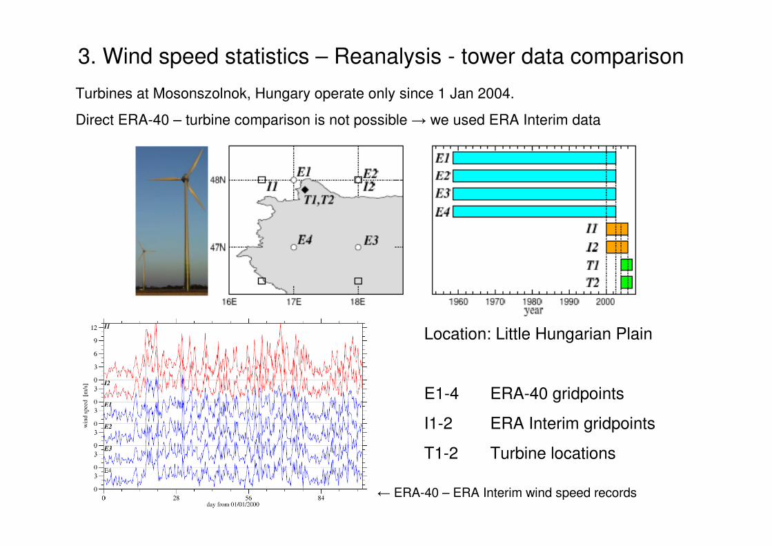
3. Wind speed statistics – Reanalysis - tower data comparison
Turbines at Mosonszolnok, Hungary operate only since 1 Jan 2004.
Direct ERA-40 – turbine comparison is not possible → we used ERA Interim data
Location: Little Hungarian Plain
E1-4 ERA-40 gridpoints
I1-2 ERA Interim gridpoints
T1-2 Turbine locations
← ERA-40 – ERA Interim wind speed records

3. Wind speed statistics – Reanalysis - tower data comparison
ERA Interim (10 m) – tower data (65 m) wind speed records
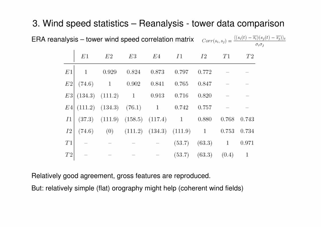
3. Wind speed statistics – Reanalysis - tower data comparison
ERA reanalysis – tower wind speed correlation matrix
Relatively good agreement, gross features are reproduced.
But: relatively simple (flat) orography might help (coherent wind fields)

3. Wind speed statistics – Reanalysis - tower data comparison
ERA Interim – turbine data: linear regression
Relatively good agreement of pdfs is reached by rescaling with 1.51 (from regression). This is close to matching the averages.
turbine (T1)ERA Interim (I1)
Note: the average empirical wind profile suggests rescaling with 1.19
A map of the scaling factor would be needed – E.ON data (?)

3. Wind speed statistics – Reanalysis - tower data comparison
Empirical probability density functions of wind speed
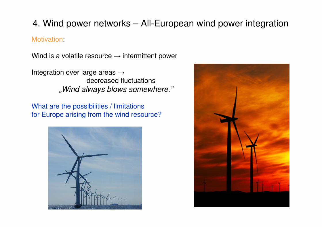
4. Wind power networks – All-European wind power integration
Motivation:
Wind is a volatile resource → intermittent power
Integration over large areas →decreased fluctuations
„Wind always blows somewhere.”
What are the possibilities / limitations for Europe arising from the wind resource?
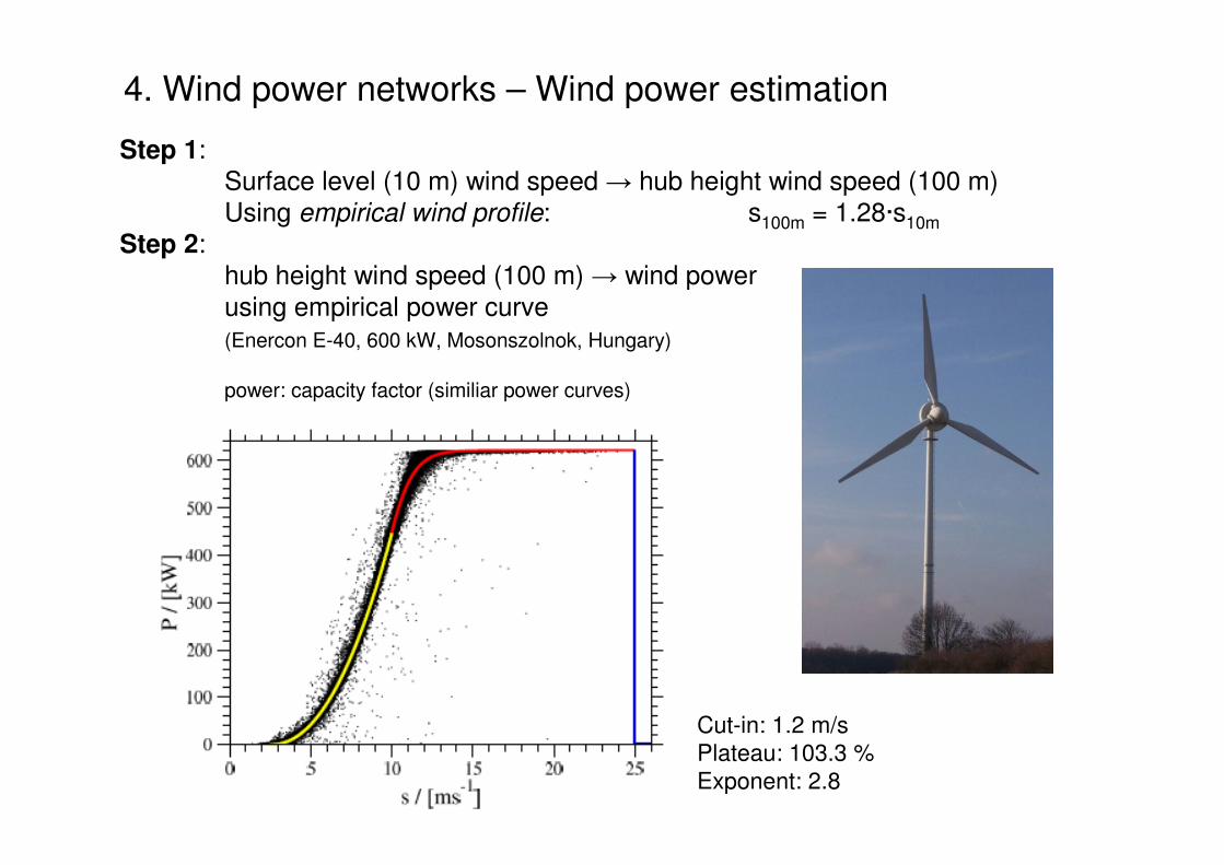
4. Wind power networks – Wind power estimation
Step 1:Surface level (10 m) wind speed → hub height wind speed (100 m)Using empirical wind profile: s100m = 1.28·s10m
Step 2:hub height wind speed (100 m) → wind powerusing empirical power curve (Enercon E-40, 600 kW, Mosonszolnok, Hungary)
power: capacity factor (similiar power curves)
Cut-in: 1.2 m/sPlateau: 103.3 %Exponent: 2.8
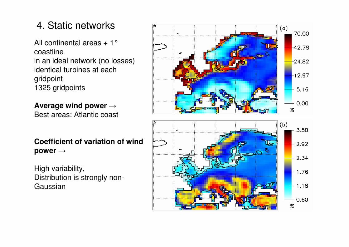
4. Static networks
All continental areas + 1° coastlinein an ideal network (no losses)identical turbines at each gridpoint1325 gridpoints
Average wind power →
Best areas: Atlantic coast
Coefficient of variation of wind
power →
High variability,Distribution is strongly non-Gaussian

Fully connected network: aggregated capacity factor
average 14.4 %, standard deviation: 6.8%
4. Static networks
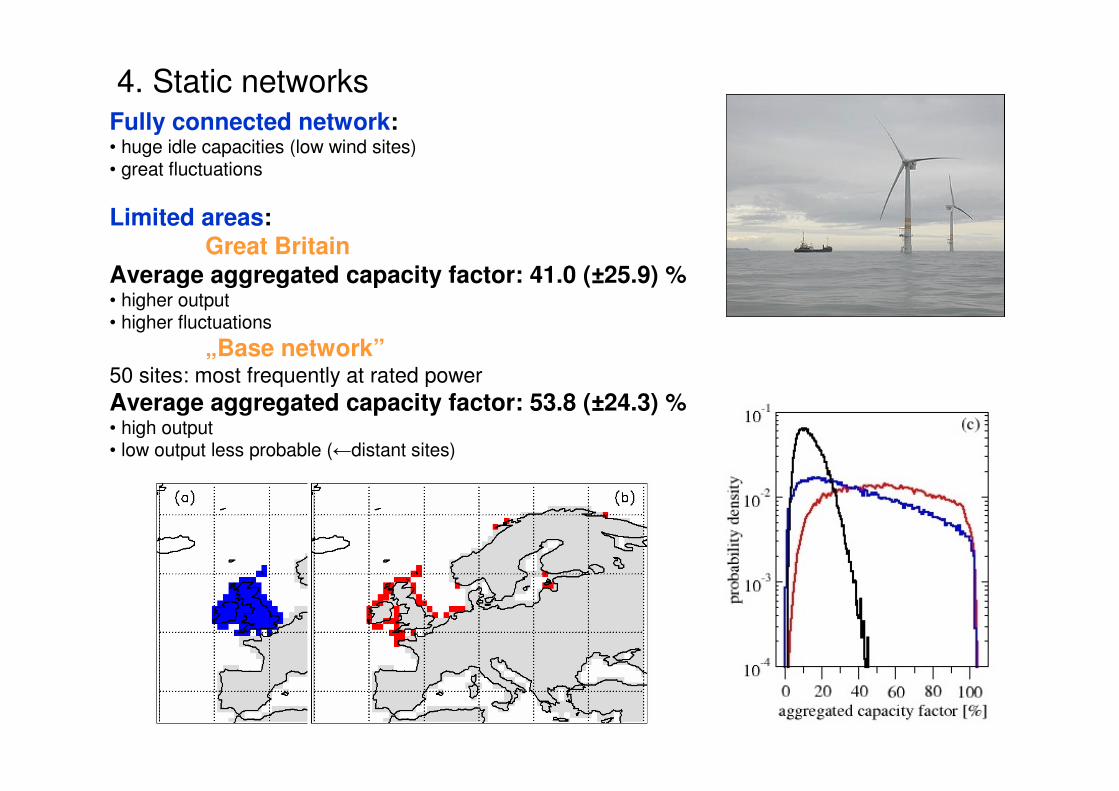
4. Static networksFully connected network:• huge idle capacities (low wind sites)• great fluctuations
Limited areas:Great Britain
Average aggregated capacity factor: 41.0 (±25.9) %• higher output• higher fluctuations
„Base network”50 sites: most frequently at rated powerAverage aggregated capacity factor: 53.8 (±24.3) %• high output• low output less probable (←distant sites)

4. Static networks
Reasons:
Characteristic time ofautocorrelations →(exp. decay)
short correlations
Characteristic length ofspatial correlations →(exp. decay)
large areas are strongly correlated
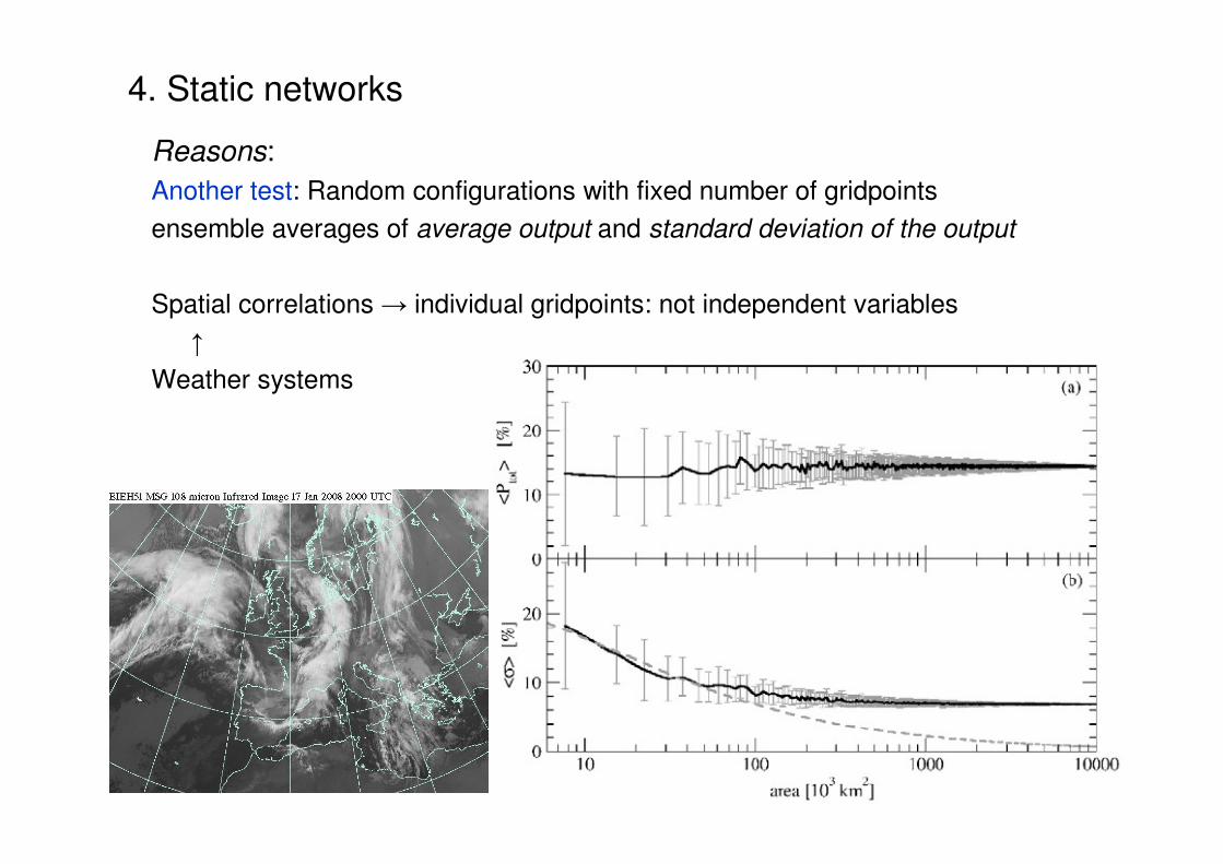
Reasons:Another test: Random configurations with fixed number of gridpoints
ensemble averages of average output and standard deviation of the output
Spatial correlations → individual gridpoints: not independent variables
↑
Weather systems
4. Static networks
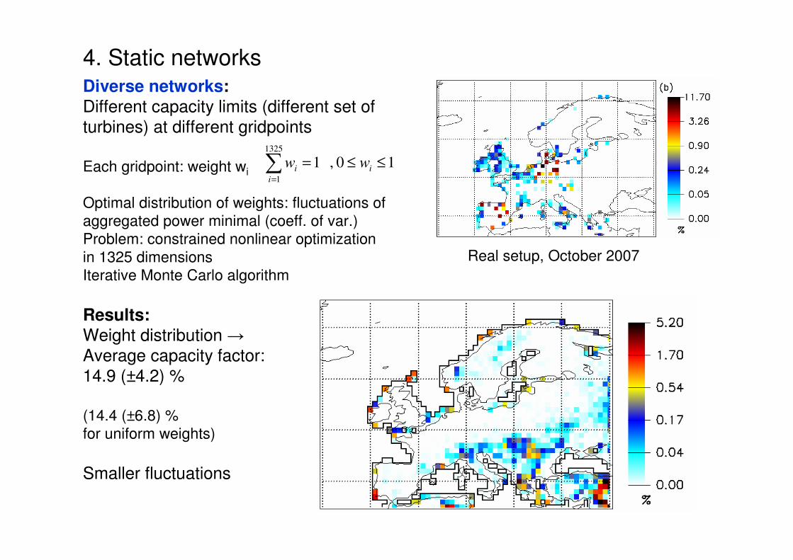
4. Static networksDiverse networks:
Different capacity limits (different set of turbines) at different gridpoints
Each gridpoint: weight wi
Optimal distribution of weights: fluctuations of aggregated power minimal (coeff. of var.)Problem: constrained nonlinear optimization in 1325 dimensionsIterative Monte Carlo algorithm
Results:
Weight distribution →Average capacity factor:14.9 (±4.2) %
(14.4 (±6.8) % for uniform weights)
Smaller fluctuations
10 , 11325
1
≤≤=∑=
i
i
iww
Real setup, October 2007

Average: all ~14%, st.dev.: 12.4% (real), 6.8% (uniform), 4.2% (optimized)
4. Static networks based on real wind farm data
Full dynamic control
Target:aggregated power output of the network should beconstant at a modest level: 50 sites (out of 1325; 3.8 %) at rated power
• ideal network (no losses)
Strategy:
sites at rated power are connected
(preferably from the „base network”)
if insufficient: best sites are connected (in the order of instantenous power)
4. Dynamic networks

Full dynamic control
Results:
• Target cannot be sustained (sudden breaks, low wind scenarios)• The whole continent should be connected (still insufficient)
4. Dynamic networks

Full dynamic control
Results: base network →
Active sites (red) and the network (blue)
4. Dynamic networks
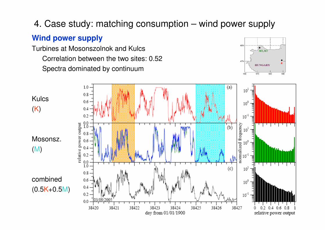
Wind power supply
Turbines at Mosonszolnok and Kulcs
Correlation between the two sites: 0.52Spectra dominated by continuum
Kulcs
(K)
Mosonsz.
(M)
combined(0.5K+0.5M)
4. Case study: matching consumption – wind power supply

Consumption
Great consumer
(factory in Hungary)
4. Case study: matching consumption – wind power supply
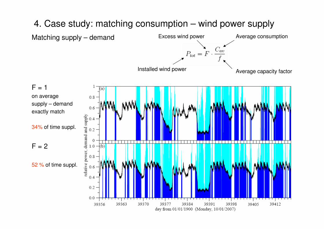
Matching supply – demand
F = 1on average supply – demandexactly match
34% of time suppl.
F = 2
52 % of time suppl.
4. Case study: matching consumption – wind power supplyAverage consumption
Average capacity factorInstalled wind power
Excess wind power

Matching supply – demand
time of supply excess (rel. to Ptot) missing power
Demand as
beforeF: 1 - 234% - 52%100% not poss.
Constant
demand
4. Case study: matching consumption – wind power supply
F
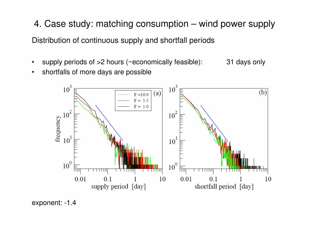
Distribution of continuous supply and shortfall periods
• supply periods of >2 hours (~economically feasible): 31 days only• shortfalls of more days are possible
exponent: -1.4
4. Case study: matching consumption – wind power supply
F
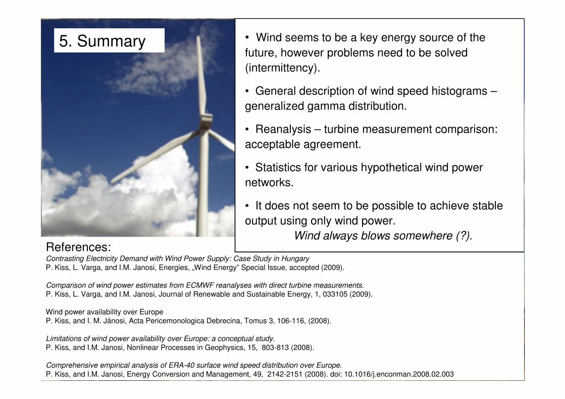
References:Contrasting Electricity Demand with Wind Power Supply: Case Study in Hungary
P. Kiss, L. Varga, and I.M. Janosi, Energies, „Wind Energy” Special Issue, accepted (2009).
Comparison of wind power estimates from ECMWF reanalyses with direct turbine measurements.P. Kiss, L. Varga, and I.M. Janosi, Journal of Renewable and Sustainable Energy, 1, 033105 (2009).
Wind power availability over EuropeP. Kiss, and I. M. Jánosi, Acta Pericemonologica Debrecina, Tomus 3, 106-116, (2008).
Limitations of wind power availability over Europe: a conceptual study. P. Kiss, and I.M. Janosi, Nonlinear Processes in Geophysics, 15, 803-813 (2008).
Comprehensive empirical analysis of ERA-40 surface wind speed distribution over Europe. P. Kiss, and I.M. Janosi, Energy Conversion and Management, 49, 2142-2151 (2008). doi: 10.1016/j.enconman.2008.02.003
• Wind seems to be a key energy source of the future, however problems need to be solved (intermittency).
• General description of wind speed histograms –generalized gamma distribution.
• Reanalysis – turbine measurement comparison: acceptable agreement.
• Statistics for various hypothetical wind power networks.
• It does not seem to be possible to achieve stable output using only wind power.
Wind always blows somewhere (?).
5. Summary