www.theigc.org

Directed and Organised by

International Growth CentreLondon School of Economics and Political Science 4th Floor, Tower Two Houghton Street London WC2A 2AE United Kingdom

For media or communications enquiries, please contact Mazida Khatun

mazida.khatun@theigc.org

a Department of Economics – University of Dar es Salaam (contact: bkmkenda@udsm.ac.tz); b International Food Policy Research Institute (contact: b.vancampenhout@cgiar.org)

Estimating Transaction Costs in Tanzanian Supply ChainsBeatrice Kalinda Mkendaa and Bjorn Van Campenhoutb

Working Paper 11/0898 November 2011

Estimating Transaction Costs in TanzanianSupply Chains

Beatrice Kalinda Mkenda

Department of Economics - University of Dar es Salaam,

bkmkenda@udsm.ac.tz

and

Bjorn Van Campenhout

International Food Policy Research Institute - Kampala

b.vancampenhout@cgiar.org

April, 2011

This paper was commissioned by the International Growth Centre (IGC) Tanzania, www.theigc.org, with funding fromthe UK Department for International Development (DfID). We would like to thank Chris Adam, Douglas Gollin, StefanDercon, Charles Kyando and the participants of the Research Workshop on Agriculture and Growth in Tanzania, 9November 2010, Dar Es Salaam, for very helpful comments. All errors remain our own.

1 The Context and Rationale

Kilimo Kwanza1 emphasizes modernization and commercialization of agriculture, which entailsimproving current technology used, and access and participation of smallholder farmers in markets.However, market participation is not costless. Transaction costs exist in all market exchange, and hightransport costs, which are an element of transaction costs2, are a major deterrent for marketparticipation of farmers in Africa, and they affect the price farmers receive3 as well as their productivity(Hine and Ellis, 2001). This implies that a reduction in transaction costs can encourage smallholderfarmers to participate in marketing of their produce. In addition, and potentially more important in thelonger run, the increased prices may trigger the farmer to review his product portfolio in the light ofthese new opportunities. As such, indirectly, the reductions of inefficiencies along the marketing chainmay lead to everlasting productivity gains through a reshuffle of the product portfolio of smallholderfarmers that better exploits their comparative advantage.

In the Kilimo Kwanza initiative, improvement in transportation has been recognized as one of the tasksin the implementation framework, where improving the rail and road infrastructure is clearlymentioned. This study is a systematic review of evidence on the scale of transport costs that Tanzaniansmallholder farmers face. Such a study is relevant as it will help to formulate policies to improve theincomes of smallholder farmers, as well as the prices that consumers eventually pay.

The agriculture sector is central to the Tanzanian economy. It provides substantial export earnings aswell as income and employment to a large number of Tanzanians. Table 1.1 shows that agriculture’sshare in GDP averaged 28.5% between 2000 and 2006 compared to an average of 19.9% of industry andconstruction over the same period. In terms of export earnings, between 2001 and 2009, Tanzania’s

1 Officially launched in August 2009, by President Kikwete, Kilimo Kwanza was initiated by the Tanzania NationalBusiness Council. It is a private sector driven resolve to accelerate transformation of Tanzania’s agriculture. TheKilimo Kwanza strategy outlines ten pillars that are important for its implementation. The ten pillars give details ofspecific tasks, activities, implementing partners, timeframes and budgets for its successful implementation (seehttp://www.tnbctz.com; accessed on March 12th 2011).2 Throughout the paper, we will frequently use the terms transaction costs, transportation costs and marketingmargin, so it is a good idea to define these here. “Transaction costs” is a broad concept that refers to all costs,material or immaterial, that one faces engaging in the process of arbitrage.” Transport costs” is much narrower (butoften large as a share) and refers to the costs incurred by transporting the goods between locations. For example, itmay be that the trader needs a short term loan to bridge the period between when he pays the farmer cash at the farmgate and when he gets the money from the wholesaler. The interest rate on this loan would qualify as a transactioncost, but would not be part of the transportation cost. Transaction costs may also be immaterial, for instance theopportunity time of waiting at a police checkpoint. As such, transaction costs are seen as more of a theoreticalconcept. One may argue that if trade of a certain good is legally prohibited, transaction costs are infinite. Finally, theterm “marketing margin” is generally used as an operational concept. Depending on the context, it refers to thedifference between seller price and buyer price (for instance farm gate price and consumer price) or the differencebetween the price of a homogenous commodity in two different locations.3 Research has shown that compared to Asia where transport costs are not as high, Asian farmers received between70-85% of the final market price, while African farmers received only between 30-50% of the final market price.Most of the difference went to transport costs (Ahmed and Rustagi, 1987, quoted by Hine and Ellis, 2001).

traditional agricultural exports4 contributed an average of 25% to total commodity export earnings (BOT,2009). The average is of course lower than that from the previous decade where the contribution fromtraditional exports averaged 60%. Exports from minerals have in recent years overtaken the contributionof traditional exports.

In terms of labour absorption, the agriculture sector employed 82.1% and 76.5% of total employment in2001 and 2006 respectively. Although the percentage has fallen somewhat, the sector is still a largeemployer of labour compared to industry which accounted for 2.6% and 4.2% of employment in thesame years.

Table 1.1 Selected Indicators2000 2001 2002 2003 2004 2005 2006

Agriculture, Hunting and Forestry 29.5 29.0 28.6 28.7 29.5 27.6 26.5Fishing 1.8 1.7 1.7 1.6 1.5 1.4 1.4

Industry and construction 17.9 18.0 19.6 21.0 20.8 20.8 21.0Services 45.3 45.5 44.2 42.7 42.0 42.5 43.8

Employment in agriculture (% of totalemployment)

- 82.1 - - - - 76.5

Employment in industry (% of totalemployment)

- 2.6 - - - - 4.3

Source: National Bureau of Statistics (NBS) (2007); World Bank (2010), World Development IndicatorsCD-ROM.

While the importance of the agriculture sector to the Tanzanian economy in terms of export earningsand employment is undisputable, the level of income of smallholder farmers (the mode of producersengaged in the sector) is low. Table 1.2 shows that although the level of food and basic needs poverty inrural areas has fallen marginally over the years, it is still higher compared to urban areas.

Table 1.2 Poverty in TanzaniaYear Dar es Salaam Other Urban areas Rural areas Mainland Tanzania

Food 1991/92 13.6 15.0 23.1 21.62000/01 7.5 13.2 20.4 18.7

2007 7.4 12.9 18.4 16.6Basic Needs 1991/92 28.1 28.7 40.8 38.6

2000/01 17.6 25.8 38.7 35.72007 16.4 24.1 37.6 33.6

Source: NBS, (2009), Household Budget Survey 2007.

4 Tanzania’s traditional agricultural exports are coffee, cotton, sisal, tea, tobacco, cashew nuts and cloves.

Given that the majority of farmers who are the backbone of Tanzania’s agriculture sector aresmallholders, examining ways in which the agriculture sector can be developed can shed light on howthe farmers’ livelihoods can be improved. In fact, the launching of Kilimo Kwanza is timely and shouldhelp to arouse a renewed interest in research to examine ways in which Tanzania’s agricultural sectorcan be revamped so that smallholder farmers can have higher incomes.

The rest of the paper is structured as follows; section two reviews literature on the importance oftransport to agricultural development, and gives an overview of Tanzania’s transport infrastructure.Section three analyses how transport costs affect marketing margins and pricing of agricultural crops,and it also presents a review of previous studies that have attempted to quantify transport costs inTanzania. Section four is our attempt to estimate transaction costs. This is done using three differentdata sources.5 First, to get an idea on how trade is organised at the local and the regional level, we didsemi-structured interviews with some traders. Next, we use a survey of semi-subsistence farmers inrural Mufindi (Iringa Region) to look at farm-gate prices. Finally, we use price series data from differentmarkets to estimate regional marketing margins. Section five summarizes the main findings.

5 It is important to clarify the key terms used in this paper. Transaction costs are broadly defined as all costs relatedto the marketing of commodities. They include transport costs, profit earned, and costs of imperfect information (seeKähkönen and Leathers, 1999). Marketing margins refer to the difference between prices in different points in themarketing chain; for example, the difference between the price a farmers gets for a 100kg bag of maize and the pricethe retailer pays for the same bag of maize, called the farm-gate-retail margin. Marketing margins are determined bytransaction cost, and a key part of transaction costs are transport costs.

2 Importance of Transport to Agriculture and the State ofTanzania’s Infrastructure

Studies have shown that economic growth and transportation are closely linked. For example, a study inthe United States indicated that areas that were linked by efficient roads and rail links dictated themovement of people and goods, and contributed to economic prosperity and expansion.6 This isbecause efficient transport networks enable transportation of goods from where they are produced tomarkets, and it also helps the movement of people. Indeed, the railroad reduced transport costs, andhence allowed markets to be integrated. The integration of markets in turn led to regional specialisationin production, which increased efficiency and stimulated growth (Eichengreen, 1994).

Agricultural products are perishable, seasonal and bulky. As such, they need an efficient and reliabletransport system to preserve their freshness and to take them to markets. Without a reliable transportsystem, agricultural products can easily rot. Besides transporting produce from farms, an efficienttransport network is also instrumental in ensuring that farmers get the required inputs needed for theirfarm activities. Thus, transportation is crucial for both taking produce to markets and for obtainingrequired inputs for production.

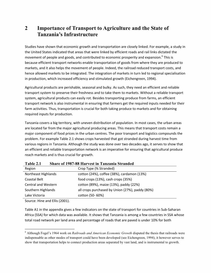
Tanzania covers a big territory, with uneven distribution of population. In most cases, the urban areasare located far from the major agricultural producing areas. This means that transport costs remain amajor component of food prices in the urban centres. The poor transport and logistics compounds theproblem. For example Table 2.1 shows crops harvested that got stranded during harvest time fromvarious regions in Tanzania. Although the study was done over two decades ago, it serves to show thatan efficient and reliable transportation network is an imperative for ensuring that agricultural producereach markets and is thus crucial for growth.

Table 2.1 Share of 1987-88 Harvest in Tanzania StrandedRegion Crop Type (% Stranded)

Northeast Highlands cotton (24%), coffee (38%), cardamon (13%)Coastal Belt food crops (13%), cash crops (35%)Central and Western cotton (89%), maize (13%), paddy (22%)Southern Highlands all crops purchased by Union (27%), paddy (80%)Lake Victoria cotton (50- 60%)

Source: Hine and Ellis (2001).

Table A1 in the appendix gives a few indicators on the state of transport for countries in Sub-SaharanAfrica (SSA) for which data was available. It shows that Tanzania is among a few countries in SSA whosetotal road network per land area and percentage of roads that are paved is under 10% for both

6 Although Fogel’s 1964 work on Railroads and American Economic Growth disputed the thesis that railroads wereindispensable as other modes of transport could have been developed (see Eichengreen, 1994), it however serves toshow that transportation helps to connect production areas separated by vast land, and is instrumental to growth.

indicators. The indicators attest to Tanzania’s need to increase its road network given that the country’sland area is vast. There is also a significant issue of Tanzania’s topography. Figure 1 in the appendixshows that Tanzania has a fairly dense network of dirt roads around the outer rim. However, much ofthe middle is empty, which results in the averages being pulled down.7

The indicators in Table A1 do not say anything about the quality of roads and rail infrastructure.However, it is public knowledge that in most developing countries, roads and rail networks are bothinadequate and are of poor quality. This is basically the environment in which goods are transported andtraded, which undoubtedly contributes to high transaction costs.

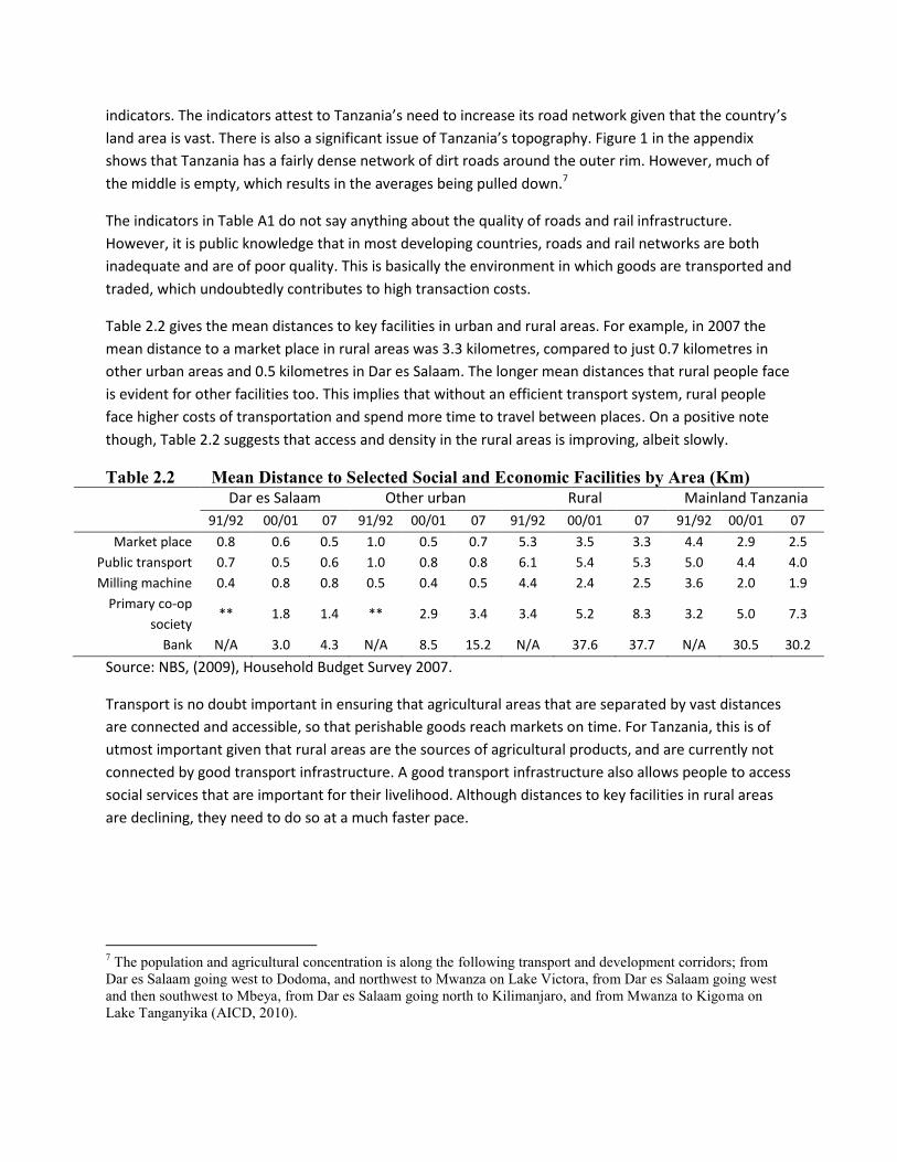
Table 2.2 gives the mean distances to key facilities in urban and rural areas. For example, in 2007 themean distance to a market place in rural areas was 3.3 kilometres, compared to just 0.7 kilometres inother urban areas and 0.5 kilometres in Dar es Salaam. The longer mean distances that rural people faceis evident for other facilities too. This implies that without an efficient transport system, rural peopleface higher costs of transportation and spend more time to travel between places. On a positive notethough, Table 2.2 suggests that access and density in the rural areas is improving, albeit slowly.

Table 2.2 Mean Distance to Selected Social and Economic Facilities by Area (Km)Dar es Salaam Other urban Rural Mainland Tanzania

91/92 00/01 07 91/92 00/01 07 91/92 00/01 07 91/92 00/01 07

Market place 0.8 0.6 0.5 1.0 0.5 0.7 5.3 3.5 3.3 4.4 2.9 2.5Public transport 0.7 0.5 0.6 1.0 0.8 0.8 6.1 5.4 5.3 5.0 4.4 4.0Milling machine 0.4 0.8 0.8 0.5 0.4 0.5 4.4 2.4 2.5 3.6 2.0 1.9

Primary co-opsociety

** 1.8 1.4 ** 2.9 3.4 3.4 5.2 8.3 3.2 5.0 7.3

Bank N/A 3.0 4.3 N/A 8.5 15.2 N/A 37.6 37.7 N/A 30.5 30.2

Source: NBS, (2009), Household Budget Survey 2007.

Transport is no doubt important in ensuring that agricultural areas that are separated by vast distancesare connected and accessible, so that perishable goods reach markets on time. For Tanzania, this is ofutmost important given that rural areas are the sources of agricultural products, and are currently notconnected by good transport infrastructure. A good transport infrastructure also allows people to accesssocial services that are important for their livelihood. Although distances to key facilities in rural areasare declining, they need to do so at a much faster pace.

7 The population and agricultural concentration is along the following transport and development corridors; fromDar es Salaam going west to Dodoma, and northwest to Mwanza on Lake Victora, from Dar es Salaam going westand then southwest to Mbeya, from Dar es Salaam going north to Kilimanjaro, and from Mwanza to Kigoma onLake Tanganyika (AICD, 2010).

3 Spatial Price Analysis and Margins in Agricultural Products inTanzania – A Review of Previous Studies

The number of studies done on transport costs in Tanzania and their effects on marketing margins arefew. In this section, we review these studies, as a first indication of effects of transport costs onmarketing margins of agricultural products. The studies reviewed focus on determinants of marketingmargins in agricultural markets, how competitive the markets are, and factors accounting for the hightransaction costs in markets of agricultural products.

Marketing margins are determined by many factors, including transport costs and how efficient andcompetitive markets are. In the late 1990s, a study by Kähkönen and Leathers (1999) illustrated theextent to which marketing arrangements are efficient by looking at marketing margins in maize andcotton markets, as well as price differences across regional markets and farms. The study also providedevidence on how competitive maize markets are by the extent to which farmers decide to whom theysell their maize, and how the price of maize is determined. Their main finding was that markets formaize were becoming less efficient since liberalization of the marketing of maize. This conclusion wasarrived at by examining how marketing margins had widened over time. They also found that therewere large and volatile price differences across regions and farms, with the margin between retail andwholesale prices of maize from Iringa (one of the main suppliers of maize) to Dar es Salaam beingconsistently positive and increasing. The estimated farm-retail price margin between Iringa and Dar esSalaam was $18.92 per ton per 100km.8

Table A2 in the appendix gives wholesale, producer and retail price differences of maize between cities.The variability in prices is large; for example between Iringa and Dodoma, in a period of a year, thedifference in wholesale prices was almost double. Producer prices differences are also large; within thesouthern highland, producer prices were double between Moinga and Mafinga. The difference in retailprices is not as large, although Dar es Salaam has the highest prices, perhaps reflecting high demand.

The study by Kähkönen and Leathers (1999) identified a number of factors accounting for hightransaction costs, as being movement restrictions, infrastructural impediments, limited access to credit,lack of storage capacity, and contract enforcement problems. The infrastructural impediments identifiedare the transport infrastructure being inadequate, roads being impassable in the rainy season, and poorquality of roads. The impediments in infrastructure raise transportation costs and limit competition andthe ability of farmers to enter in marketing of maize (p.66-67). When farmers are unable to entermarkets, they become limited in selling their produce to buyers or traders who come to them who canafford the high costs of transport, or they simply choose to produce for their subsistence needs.

8 The actual estimated farm-retail price margin from the Kähkönen and Leathers (1999) study is $0.950 perkilogram. We translate it to a broadly common way of reporting that we adopt in this paper (per ton per 100km).Since the distance between Dar es Salaam and Iringa is 502 kilometres, the farm-retail price margin is $18.92 perton per 100 km (= (1000*0.950)/5.02).

This is further supported by the study findings relating to how competitive maize marketing is. Figure 3.1shows that while half of the farmers managed to get the best price, the other half were not able to get acompetitive price for their maize because they sold to the only buyer they could find or they knew. Nothaving as many buyers as farmers would want implies that they sell to a few or perhaps just one buyerand hence they do not get the best price. Lack of sufficient buyers for their produce reflects theinsufficient transport facilities to enable buyers to make the trip, or for farmers themselves to engage intransporting their own produce to markets where they can get a better price.

Figure 3.1 Percentage of Farmer and their Decision to Sell

Source: Kähkönen and Leathers (1999).

Infrastructural impediments can also manifest themselves in the way prices are determined. If transportcosts are not substantial, farmers could afford to take their crops to markets that would guarantee thema good price. However, in the face of bad roads and high transport costs, farmers have no incentive toincur such high costs, and would simply wait for buyers to get to them. When buyers incur these costs,they are likely to offer low prices to farmers. Thus, in the end, high transport costs translate in farmersgetting lower prices for their produce. Figure 3.2 shows that only 20% of the sampled farmers were ableto negotiate a price for their maize.

Figure 3.2 Price Determination of Maize

Source: Kähkönen and Leathers (1999).

Another study by Eskola (2005) estimated the marketing margins along the national supply chain forvarious agricultural products. The estimates are given in Table A3 in the appendix. The marketingmargins are much higher further along the supply chain, going as high as from 20% to 70% for an orangeretailer, compared to grain whosalers, rice brokers and regional traders whose marketing margins donot go beyond 20%.The higher marketing margins along the supply chain is explained by the long supplychains. It is not surprising that brokers are used extensively, mainly to reduce transaction costs. Thedrawback of using brokers is that the supply chain becomes longer, which has implications on the timeand money involved in trading (Eskola, 2005, p.19).

Although the study did not provide estimates of transport costs per product, it estimated the actualcosts of transporting a truck from Dar es Salaam to all regions of Tanzania, and these estimates are givenin Table A4 in the appendix. There is a high correlation between distance and cost of transportation, of0.91. Of course distance is not the only component of cost; other factors such as quality of the road, costof fuel (being higher the more remote the location is), and possibility of shipping something back fromDar es Salaam account for these costs (Eskola, 2005, p.25). The estimated costs (per ton per 100km)range from a low of $3.54 between Iringa and Dar es Salaam, to a high of $12.54 between Dar es Salaamand Mtwara. The high cost of transport between Dar es Salaam and Mtwara is explained by the poorcondition of the road.

High transport costs do not just affect internal trade of agricultural crops. For countries like Tanzania italso affects exports of agricultural crops, making high transport costs a significant impediment to thecompetitiveness of exports. Kweka (2006) estimated both land and sea transport costs for fairlyaggregated sectors. Table A5 in the appendix gives the estimated costs of domestic land costs of broadsectors relating to agricultural and non-agricultural products. Overall, Table A5 shows an increase in landfreight rates across the sectors over the period. The land freight costs rose from about 4% to almost 7%between 1998 and 2002, attributed to an increase in rail freight rates in 2001.9 The estimatedinternational freight rates (not reproduced here) showed a slight decline between 1998 and 2002,attributed to a rise in competition following the liberalisation of the freight industry (Kweka, 2006). Thedownward trend is of course encouraging to the export sector, and it would be interesting to examinewhether this trend has continued to go down.

Rapsomanikis and Karfakis (2007) used cointegration analysis on regional prices in Tanzania, with furtherexamination of threshold effects in a number of well-connected and remote markets. Their study foundno systematic pattern of the effect of transport costs on prices across Tanzania. A further test usinglinear cointegration hypothesis supported the hypothesis, suggesting that transport costs do notprevent arbitration and the transmission of price signals between markets. Both results arecounterintuitive given the poor transport infrastructure in the country. This made them to further modelthe effect of transport costs on margins, since distance and high cost of transport is endemic to

9 The freight rates are charges per unit value obtained from the Tanzania Railway Corporation. To get estimates forthe total costs, data on technical coefficients for the transport and communication services as a share of output ofeach sector was obtained from the 1992 input-output table. A price index for the freight cost was then computed foreach good. The rate of change got from the price index was then used to update the freight rate per value to get anestimate of the ad valorem freight rate for each year (see Kweka, 2006).

developing countries. They did this by spatial price analysis, which involved isolating variables thatdetermine the farm-gate-market price spread. For example, distance from either the market or thatcovered by the trade, the per unit cost of transport, number of traders, and specific household or tradercharacteristics. They employed the approach on maize, beans, coffee and banana prices. They foundsupport for the fact that wholesale farm-gate price margins are affected by transport infrastructure,distance, as well as by the competitive conduct of traders. However, the study did not measure theexact extent of the margin.

Besides affecting competitiveness, high transport costs affect margins in that traders offer low prices tofarmers, while consumers face high retail prices. Morrissey and Leyaro (2007) estimated the magnitudeof marketing margins of cash crops, food crops, and staple foods. Table A6 in the appendix showsestimates of the marketing margins, and it shows that food crops (rice and maize) in general have highermarketing margins owing to them being traded in the national markets, specifically in Dar es Salaam,where they compete with imports. The marketing margins for cash crops have declined since the early1990s, but are still high at 10%. Cash crops are exported, with local consumption consisting of a smallpercentage that is processed. The marketing margin on staple foods (cassava and bananas) is small,owing to them being traded close to where they are produced, and as such transport costs are not a keyfactor in pricing them.

In a more recent study of asymmetries in price transmission in maize marketing in Tanzania, Mduma andKipsat (2009) investigated maize prices in six regional markets (Dar es Salaam, Arusha, Mwanza, Songea,Mbeya, and Sumbawanga). When there is asymmetry in the transmission of prices, it means thatcorrelations between prices in spatial locations differ depending on the direction of changes in prices,whether down or up. Asymmetry in price transmission can indicate inefficiencies in marketing, and itcan be caused by trade restrictions, transaction costs, market power, different adjustment costs facedby producers depending on whether prices are rising or falling, and the perishable nature of products(see Rapsomanikis et al, 2003; Agra CEAS Consulting, 2007). Understanding asymmetry in pricetransmission is useful in informing policymakers when to make the right intervention (Mduma andKipsat, 2009).

The study by Mduma and Kipsat (2009) used monthly data covering the period from January 1997 toApril 2005, and Dar es Salaam was taken as the basis of comparison, given that it is the largest maizeconsumer market. They found that there was significant asymmetry in the transmission of price signals,with the correlations for upward movement of prices being stronger than those for downwardmovement of prices. In general, geographical distance and communication network explained the co-movement of the pairs of prices. For example, the strongest correlation was found between Dar esSalaam and Arusha, and the weakest correlations between Dar es Salaam and Sumbawanga, and Dar esSalaam and Songea. This is explained by the close proximity of Dar es Salaam and Arusha, and theremote locations of Sumbawanga and Songea. Geographical distance could not however explain theweaker correlation that was found between Dar es Salaam and Mbeya compared to that between Dar esSalaam and Mwanza. The explanation in this case lies in the better communication network betweenDar es Salaam and Mwanza.

The following can be drawn from the studies reviewed in this section; transport costs affect themarketing margins of agricultural products. The marketing margins are higher as more brokers are usedin the supply chain, the less competitive the markets are, the poorer the condition of the road, and thehigher the cost of fuel. Transport costs to different regional centres are determined by the condition ofthe road and distance. The more remote the area and the poorer the condition of the road, the higherthe transport cost per ton per 100km. Marketing margins also vary across types of agricultural products.Foods crops that are traded in national markets such as rice and maize have higher marketing marginsthan staples that are traded locally, such as bananas and cassava. Transport costs also affectinternational trade, although competition and liberalisation in the freight industry helped to reducefreight rates. While research found that freight rates fell marginally between 1998 and 2002, it isimportant that their reduction is further encouraged to enhance trade. The condition of roads andproximity of locations are also important in price transmission, which is crucial for policy intervention.

4 Transaction Costs in Tanzania

In this section, we try to come up with our own estimates of transaction costs in Tanzania. To do so, wehave used three different data sources. The first source of information came from traders. We organizedsemi-structured interviews with a total of 12 traders. This gave us an idea of how the maize trade wasorganised. The second source of information came from semi-subsistence farmers. We surveyed 1134households on their maize and beans marketing behaviour over one agricultural year and compared theprices they get with prices in consumer markets from different sources. Third, we used price series datafrom different regional markets to estimate transaction costs in regional trade.

4.1 Traders perspective

We organized individual semi-structured interviews with 12 traders, all located in the Mufindi District,Iringa Region, Tanzania. Most of the traders were small-scale traders, operating at the village level. Wealso interviewed 3 wholesale traders that link the small-scale traders to the regional market system (seeSection 4.3). The small-scale traders were sampled in the same villages as the ones we used in thesurvey (see Section 4.2). The wholesale traders were located in the terminal markets for these villages(Makambako and Mafinga). The interviews were conducted in October 2010. At that time, the exchangerate was about Tsh.1498 for a dollar.

The survey area, the district of Mufindi, has 133 registered villages. Mufindi has an estimated populationof about 320,000, with a population density of 45 inhabitants per square kilometre. The dominant tribein the district is the Hehe tribe. The staple food of the Wahehe is maize, which they mill and then use tocook porridge (ugali). The two most important minority tribes in the region are immigrants from Njombe(the Wabena) and Makete (the Wakinga). The district can be divided into three agro-ecological zones:the highlands (between 1,700 and 2,200 metres), the middle zone (generally referred to as the Mufindiplateau, between 1,700 and 2,000 metres) and the low plateau (between 1,200 and 1,500 metres). Thefour villages sampled are situated on the Mufindi plateau. This plateau is characterized by gently rollinghills, with wide ridges and valleys. It has low inherent soil fertility, but reasonable physicalcharacteristics. Average rainfall is between 900 and 1,200 millimetres per year. The averagetemperature is between 20 and 25 degrees Celsius. The district’s capital is Mafinga, which lies along themain road connecting Dar es Salaam to Zambia and Malawi. Makambako lies along the same road,about 70 kilometres west of Mafinga.

In general, most of the traders we interviewed traded in maize. Some also traded in beans in addition tomaize. Traders give different reasons why they started a business in maize trade, and not somethingelse. One of the reasons given is that maize is a common product in the region and hence the tradershave experience with it. Often, they cultivate it themselves or have been cultivating it in the past. Thefact that it can be stored was also a reason, as well as the fact that it is not easily destroyed (comparedfor instance to tomatoes). Also, it was mentioned that it is easily available in the village, considering thatmaize is a staple that is consumed by all villagers. This also means that it is easily sold. It was also

mentioned that the buyers of maize (often wholesale traders) are very reliable. Lastly, some traders alsoengage in maize trade because it requires relatively little capital.

Most of the traders engage in trade in several neighbouring villages, apart from their own village. Theymostly buy directly from farmers, but sometimes they buy themselves from even smaller traders. Thetrader we interviewed in Ikongosi sells to Mr. Sanga, who is a wholesaler located in Mafinga market. Hethen sells further to small traders who sell to Mafinga residents in Mafinga market. Other similarwholesalers were identified by other traders, namely Mr. Kukudesanga in Makambako. This trader usedto be a middleman who bought from villages himself and sold to wholesale traders at Makambako.However, after some time, he built up a reputation and small traders started to collect maize and bringit to him. Local traders not only sell to maize traders, but also to processors. Processors mentionedwhere IB Sembe, DC Sembe and Saadani Super Sembe. These processors mill the maize and repackageit.

The way in which a transaction materializes differs by trader. For instance, the trader in Ikongosi firstcommunicates with farmers to see if they are ready to sell. He then compares prices quoted by thefarmers to the prices in terminal markets. He then looks for a person that he can trust to go and look atthe maize. If quantity, quality and price are as agreed, this person gets back to the trader and getsmoney to collect the maize. All this is done by bicycle. Another trader narrated that he is known by thefarmers, and as such, farmers contact him (by phone, and through friends and family). Yet anotherfarmer notes that farmers are in urgent need of money after harvesting and inform him that they havemaize for sale. He then goes to check the quality and quantity himself. He then sends someone to collectthe maize. He states that the price is always dictated by him. For all the checking, this trader uses amotorbike, which he rents at about 5 dollar per day. In general, traders mention that sometimes theentire transaction is done over phone. If farmers have no phone, the trader will go and check himself.Big traders mainly work through mobile phones.

The quality of maize is judged by the colour, the weight and the hardness of the maize kernels. Beforeloading, the kernels are spread on a mat in the farmer's house, to check if there is not too much dirt andstones in the maize. Traders do not pay the agreed price if the quality is poor. They will either take itback or renegotiate the price. Grading is also facilitated by the fact that traders often employ people topick up the maize who know what quality the trader wants. It is also argued that the farmers knowthemselves what quality they are expected to deliver. Traders who buy repeatedly from the samefarmers also know what quality they can expect.

With respect to the quantity, there seems to be little room for disagreement. The standard measure formaize is a debe or tin10. These days, debes are available everywhere, and both the trader and farmer willhave one with them when they make a transaction. This to avoid that traders use debes that are largerthan the standard (rumour has it that some traders fill their debe with hot sand, which makes the debe,that is made of plastic, expand) or that farmers use debe that are smaller than the standard (by cutting asmall piece diagonally from the side of the debe and then carefully reattaching it). Traders come with

10A debe is a 20 litre bucket, which amounts to about 18 to 19kg of maize. Maize is collected and transported inbags. The number of debe per bag varies, but a standard bag would have 7 debe and weigh +/-130kg.

empty bags and fill the bag. Generally, a bag costs about Tsh.700 (about 50 cents) and it costs aboutTsh.100 (0.06 US$) in terms of labour to fill a bag.

Hauling maize within the village is done by bicycles. Once there is enough maize, either pick-ups ortrucks are used to take the maize to a regional market. Sometimes a truck picks up maize in severalvillages, and the cost is shared. We have also heard of a trader that uses an ox-cart within the village.Buses are seldom used, only if there are very few bags to be transported. It was mentioned that becauseof the poor state of the roads, truck owners ask significant fees, and the fees increase if roads get poorerduring the rainy season. None of the traders we interviewed owned trucks; transportation is provided bya third party. Unfortunately, we did not get estimates for these services from the traders directly.However, we did include some questions on access to transport from farmers in the survey. While this islikely to overestimate the cost, it gives us at least some idea of the relative costs. Table 4.1 givesestimates from the different villages to the two market centres for different modes of transport.

Table 4.1 Estimated Costs of Different Means of Transport

Cost (US$) from village to MAFINGAIBWANZI IKONGOSI IPILIMO KWATWANGA MTAMBULA MTILI NUNDWE

Distance: 75 km 25 k ? ? ? 20 km 42 kmmotorbike 13.58 4.40 16.47 16.65 15.15 5.56 9.89sedan 40.98 11.91 38.90 40.07 37.10 13.30 19.79pickup 60.79 23.55 54.21 43.89 52.94 23.68 32.96lorry 103.14 42.89 91.23 58.49 70.69 39.74 61.89

Cost in (US$) from village to MAKAMBAKOIBWANZI IKONGOSI IPILIMO KWATWANGA MTAMBULA MTILI NUNDWE

Distance ? ? 35 km 86km 47 km ? ?Motorbike 23.85 11.01 9.45 14.80 11.87 12.18 18.82Sedan 78.38 25.71 23.91 32.61 27.93 32.96 38.95pickup 99.12 44.60 39.12 38.25 40.36 53.20 73.55lorry 152.40 69.98 60.97 56.61 56.34 87.00 113.99

Note: entries are average cost reported by farmers to rent a vehicle to go to the market centre. Datacome from the farmer survey (see section 4.2) carried out in august 2008. The exchange rate at thattime was 1157.5.

Insurance does not exist, either at the village or regional level. The primary reason mentioned for theabsence of insurance was that the capital involved is too low. Furthermore, traders report limitedknowledge on (the existence of) insurance instruments. Any loss incurred is borne by the tradersthemselves. Losses do happen from time to time. One wholesaler from Makambako reported that onenight his watchman failed to turn up. That night, everything was stolen out of his storage facility.

The amount of hired labour involved in the maize trade is minimal. Persons that collect the maize atvillage level get about Tsh.400 (25 cents) per bag collected. If they work hard, they can get 4 bags a day.For bagging, loading and offloading, traders also hire workers.

Capital is provided out or the traders’ own pocket. Some people use savings. One trader indicated heused sell tea, and after he saved Tsh.70000 (about 45 US$), he started trading in maize. Another villagelevel trader inherited an ox-cart, which he lends to other villagers. The villagers paid him with maize. Assuch, he rolled into the business. Most of the village level traders reported that there is no need forloans, because of the relatively small amounts involved.

The two regional traders we interviewed did get loans. One got a loan of Tsh.8,000,000 (US$5340) fromMufindi Community Bank (MuCoBa), a micro finance service provider based in Mafinga town. Hereported paying 24% interest on this loan. This wholesaler is also a processor. The wholesaler fromMakambako got a loan from Tsh.3,000,000 (about US$2000) from a Rotating Savings and CreditAssociation (ROSCA)-type trading group. He did not have to pay interest.

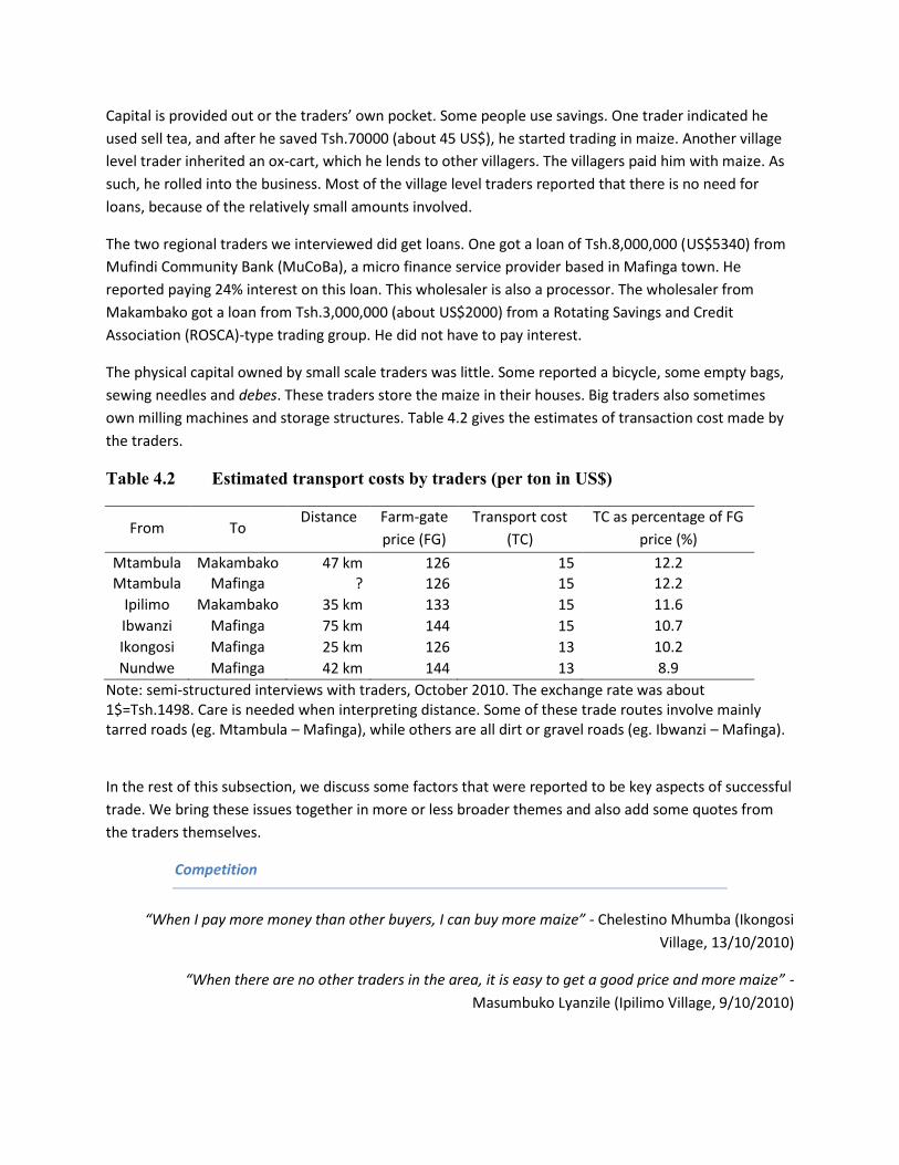
The physical capital owned by small scale traders was little. Some reported a bicycle, some empty bags,sewing needles and debes. These traders store the maize in their houses. Big traders also sometimesown milling machines and storage structures. Table 4.2 gives the estimates of transaction cost made bythe traders.

Table 4.2 Estimated transport costs by traders (per ton in US$)

From ToDistance Farm-gate

price (FG)Transport cost

(TC)TC as percentage of FG

price (%)

Mtambula Makambako 47 km 126 15 12.2Mtambula Mafinga ? 126 15 12.2

Ipilimo Makambako 35 km 133 15 11.6Ibwanzi Mafinga 75 km 144 15 10.7Ikongosi Mafinga 25 km 126 13 10.2Nundwe Mafinga 42 km 144 13 8.9

Note: semi-structured interviews with traders, October 2010. The exchange rate was about1$=Tsh.1498. Care is needed when interpreting distance. Some of these trade routes involve mainlytarred roads (eg. Mtambula – Mafinga), while others are all dirt or gravel roads (eg. Ibwanzi – Mafinga).

In the rest of this subsection, we discuss some factors that were reported to be key aspects of successfultrade. We bring these issues together in more or less broader themes and also add some quotes fromthe traders themselves.

Competition

“When I pay more money than other buyers, I can buy more maize” - Chelestino Mhumba (IkongosiVillage, 13/10/2010)

“When there are no other traders in the area, it is easy to get a good price and more maize” -Masumbuko Lyanzile (Ipilimo Village, 9/10/2010)

“When we have various buyers [at the terminal market] is when the price becomes good” - Esko IddMtoya (Ibwanzi Village, 11/10/2010)

Competition between middlemen at the village level seems to be healthy. Maize buying at the villagelevel does not seem to suffer from monopsony tendencies. In most villages, traders report that there areseveral other agents who are engaged in the “business of buying up maize”. The numbers ofcompetitors range from 5 in Mtambula to more than 20 in Ikongosi. While the majority of buyers arefrom within the village, traders from other villages or even towns are allowed in the villages. Tradersfrom outside the village are required to report to the village government first, where they usually haveto reveal the price at which they are willing to buy the commodity. We did not learn of any disputesbetween buyers from within the village versus buyers from outside the village. There are differentreasons why there are many traders in these villages. One of the main reasons mentioned is thatentering the market does not require huge amounts of capital

Market conditions

“When farmers need money for school fees, etc., I can buy much and sometimes at cheap prices” - KanutiLutego (Ipilimo Village, 9/10/2010)

“If at the market there is a shortage of maize [at the terminal market], I make profit because I decide onthe price of maize” - George Chengula (Makambako, 15/10/2010)

“If I get information on good prices and if I have stocked maize, I make good business” - Titho Kabonge(Nundwe Village, 14/10/2010)

Local demand conditions, both in the village and at the terminal market, provide the reference prices forthe traders. From the buyer's point of view, traders report to make more profit when there is sufficientsupply of maize in the villages. This is often the case immediately after the harvest or in periods whenlarge sums of money are needed (for instance, when school fees have to be paid). From the seller's pointof view, traders report that they can dictate (higher) prices if there is a shortage of maize in the terminalmarket. Note that market conditions are closely related to competition, as excess supply at the locallevel and excess demand at the terminal market may be the result of insufficient middlemen.

Information

“When farmers have no information on the price of maize in other villages, I can get maize at cheaperprices. That is when I make good business” - Kanuti Lutego (Ipilimo Village, 9/10/2010)

“If farmers do not know the price where I am selling, I can make more profit” - Method Nyondo(Mtambula Village, 9/10/2010)

Price information seems to be very important for traders. It was mentioned as a key determinant ofprofits by 5 of the 12 traders interviewed. Price information is relevant for both buying and sellingmaize. Traders report higher margins are possible if the farmers do not know the current reference

prices (eg. price in terminal markets, and prices offered by other traders). In other words, middlemen doseem to exploit information advantages if they have it. In addition, price information is also importantwhen selling the maize. It enables traders to maximize returns on both spatial and inter-temporal (seealso market conditions above) arbitrage.

Taxes

“If I don't pay local taxes on the way to the market is when I make profit”- Masumbuko Lyanzile (IpilimoVillage, 9/10/2010)

Traders usually have to pay taxes to the local government, and these have also been reported as criticaldeterminants on the profits they can make. The official tax rates reported by the Tanzanian RevenueAuthority are 4% for residents and 15% for non-residents for overland transport(http://www.tanzania.go.tz/tra.html). However, in reality, the rates differ from village to village. In ourfieldwork, they range from Tsh.500 (about 33 cents) to Tsh.1500 (about 1 US$) per bag. Traders shouldget an official receipt upon paying taxes, which they should be able to show at potential checkpointsalong the road to the terminal market. Some traders try to avoid these taxes by leaving the villageunnoticed, but this may undermine future relationships with the local tax authorities. What alsohappens often is that traders pay local taxes without requiring a receipt. This is a mutually beneficialarrangement for both the tax receiver and tax payer (as the receiver just puts this in his pocket and thetax payer gets a reduced rate). But then there is still the possibility that the trader gets caught furtherdown the road, possibly incurring an additional fine. In sum, the decision to pay local taxes or not seemsto be a complex optimization problem involving the tax rate, the probability of being caught at differentcheckpoints, future interactions with tax authorities and the expected amount needed to bribe officialsat the village and/or different checkpoints.

Trust

“I make good business if I get maize at a cheap price. To achieve this, I must go to the farmers with cashin hand and go house to house. In so doing, farmers are willing to sell maize as they are sure money is

paid on the spot” - Kilindapi Mahenge (Mtambula Village, 9/10/2010)

“When I have no money but still the farmer gives maize on loan, that is when I make business”- Esko IddMtoya (Ibwanzi Village, 10/10/2010)

Some farmers also mentioned that trust was important for a successful business in maize trade. Lots oftraders deal with the same farmers year after year. As was mentioned before, this means that there is amutual understanding on the quality of maize that should be delivered.

Quality control

“If I make follow up of the farmers on the quality of maize, this is when I get higher profit”- MidanoOneza (Mafinga, 16/10/2010)

While the quality of maize seems to be relatively easy to check, some traders did mention that followingup on the farmers could improve the maize.

In sum, the trader survey reveals that transport costs vary between around 0.2US$ and 0.5US$ per kmper metric ton. Hired labour and own capital used in local trade is minimal. Competition at the villagelevels seems good, with lots of agents of agents engaged in maize trade. The market conditions alsoseem favourable, with frequent transactions going on throughout the year. Traders do sometimes seemto exploit the price information advantage when dealing with farmers. Local taxes are reported to be animportant impediment to trade. There are also some minor issues with respect to trust and qualitycontrol, but these are often reduced by frequent personal interactions between the different parties.

4.2 Smallholder farmers perspectives

In August 2008, a purposely designed survey to better understand marketing behaviour of smallholderfarmers in the Mufindi District, Tanzania, was carried out, as part of a broader research project(Lecoutere et al. (2010); D'Exelle et al. (2010)). While the main focus was on maize, detailed informationon production and marketing of beans was also collected. We can use the difference between pricesreceived by the farmer and the price in the terminal markets to infer transaction costs on a local level.

Mufindi District, which is located in Iringa region, was chosen because of the importance of maize in theproduction system of the farmers. Iringa region, and especially Mufindi, is a main maize production areathat supplies the rest of Tanzania, as well as Malawi and Zambia (see also Kähkönen and Leathers(1999)). Within the region, we chose 7 villages. These villages were selected to maximize distance toterminal market (Mafinga, the district capital) and agro-climatic conditions. Within each village, werandomly selected households pro rata the size of each village. In total, we interviewed 1134 farmers attheir homes. The breakdown of respondents by village is given in Table 4.3.

The first striking feature is that few farmers seem to participate in the market in terms of maize or beanssales. For maize, only 38 percent of the interviewed farmers report having sold once or more during theprevious year. While all farmers produce maize, 12 percent of the framers did not grow beans. Of theones who did, only 36 percent report sales transaction(s) over the last 12 months.

Table 4.3 Villages and Number of Respondents

VILLAGE NUMBER OF RESPONDENTS

IBWANZI 189IKONGOSI 143IPILIMO 157KWATWANGA 169MTAMBULA 166MTILI 161NUNDWE 149

Disregarding all households that did not participate by selling to the market, we recorded a total of 493separate maize transactions and 384 beans transactions. So another interesting finding is that mostfarmers opt to sell everything at once instead of selling smaller quantities at different points in time.There is only one farmer that reports 5 separate maize transactions during the last year. For beans,virtually everybody reports only one occasion where they sell. Given the high variation of prices over thecourse of an agricultural year (see below), and the associated price risk, it seems strange that farmers donot spread price risk by selling at different points in time. One possible explanation may be that farmersare limited to only a few selling opportunities (eg., traders only visit the village once a year). Anotherreason may be that, in the absence of consumer credit, farmers are obliged to sell everything at once tomeet urgent expenditures.

The above contrasts with high variability in the amounts marketed by the farmers: while mean sales ofmaize is about 462.5kg, the standard deviation is as high as 450kg. There is even one farmer who reportsa single transaction of more than 8 tons! Even when we discard some potential outliers at the upper endof the distribution, we remain with standard deviations that far exceed the mean. For beans, theaverage transaction is just over 76kg, but also with a significant standard deviation (about 100kg).

Before we turn to the most interesting aspect of smallholder maize marketing, the prices, let us brieflylook at the timing of harvests and sales. Figure 4.1 gives 4 basic bar charts, and cover one agriculturalyear for maize. The first panel (a) reports the timing of the maize harvest. As can be seen, most farmersharvest in August or September. From April to July, we also observe a gradual onset in maize harvesting.While most of this can be accounted for by differences in the agro-climatic conditions (for instance, inKwatwanga, which lies in a hotter and dryer area, 85 percent of farmers harvest before August), thismay also suggest some farmers harvest their maize prematurely.

The second panel (b) reports timing of sales transactions. As can be seen, the bulk of transactions takeplace immediately after the harvest, mainly between September and December. The high variability inthe amounts sold by the farmers is illustrated in panel (c). The last panel (d) presents a bar plot of thetotal number of debes sold. The highest total quantities are recorded in November and December withslightly less than 2000 debe, which amounts to 37 tons.

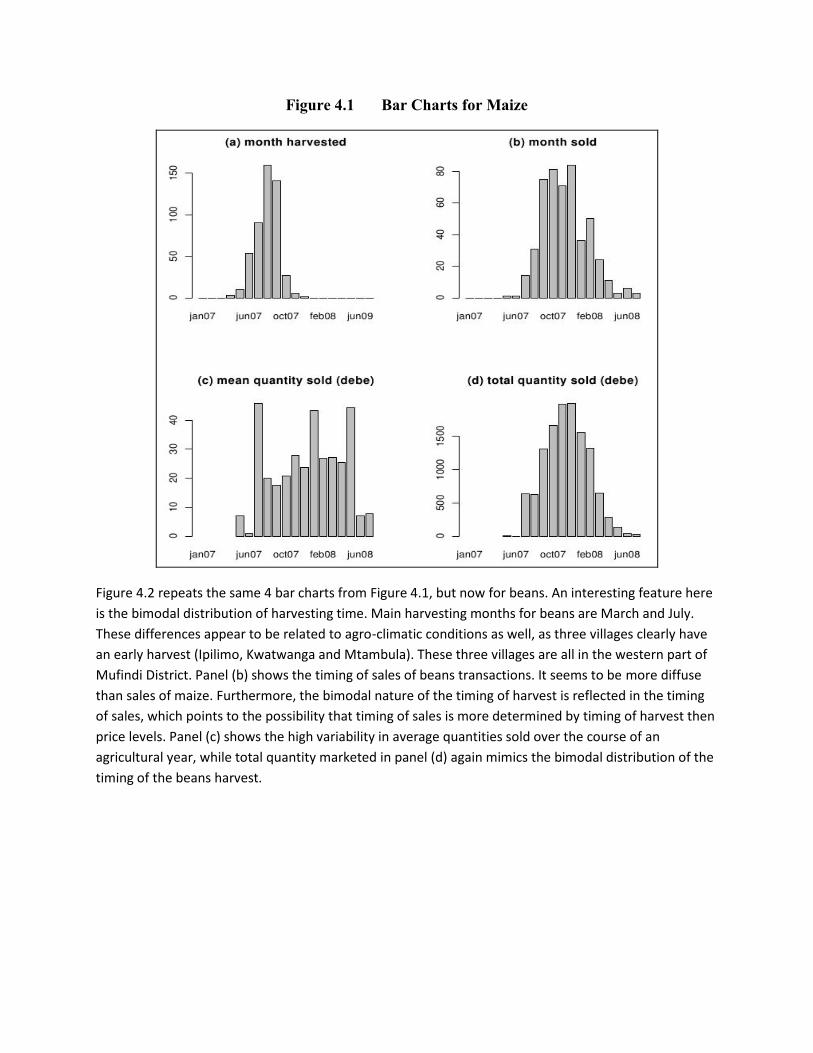
Figure 4.1 Bar Charts for Maize

Figure 4.2 repeats the same 4 bar charts from Figure 4.1, but now for beans. An interesting feature hereis the bimodal distribution of harvesting time. Main harvesting months for beans are March and July.These differences appear to be related to agro-climatic conditions as well, as three villages clearly havean early harvest (Ipilimo, Kwatwanga and Mtambula). These three villages are all in the western part ofMufindi District. Panel (b) shows the timing of sales of beans transactions. It seems to be more diffusethan sales of maize. Furthermore, the bimodal nature of the timing of harvest is reflected in the timingof sales, which points to the possibility that timing of sales is more determined by timing of harvest thenprice levels. Panel (c) shows the high variability in average quantities sold over the course of anagricultural year, while total quantity marketed in panel (d) again mimics the bimodal distribution of thetiming of the beans harvest.

Figure 4.2 Basic Bar Charts for Beans

Let us now look at the prices at which farmers sold their products. Overall, a debe of maize was sold atTsh.4687 (about US$220 per ton), while a debe of beans was sold at Tsh.10850 (about US$500 per ton).However, such an average over the entire agricultural year hides important month-to-month pricevariability, especially since our observation period covers the 2007-2008 global food crises.11 In Figure4.3, we present time series data of average prices of maize (panel (a)) and beans (panel (b)) sold in eachmonth of the agricultural year.12 As can be seen, for both commodities, the prices more than doubledover the agricultural year. More specifically, the studentized range for maize is 3.6, while that for beansis 3.2!

11 Between March 2007 and March 2008, global food prices increased an average of 43 percent, according to theInternational Monetary Fund. During that time period, wheat, soybean, corn, and rice prices increased by 146percent, 71 percent, 41 percent, and 29 percent, respectively, according to the U.S. Department of Agriculture(Carcani, 2010).12 The representativeness of these prices should be judged by looking at panel (b) in Figure 4.1 and 4.2. Forexample, for maize, the mean prices in June and July in both 2007 and 2008 are based on only a few observations.

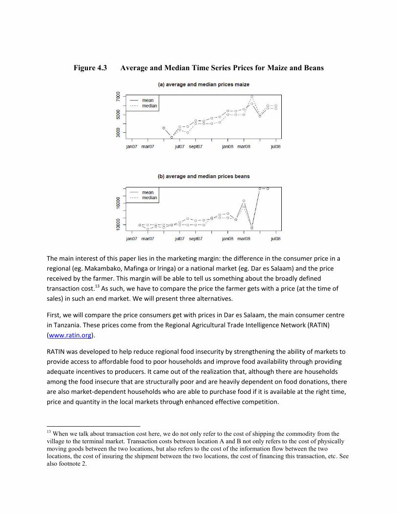
Figure 4.3 Average and Median Time Series Prices for Maize and Beans

The main interest of this paper lies in the marketing margin: the difference in the consumer price in aregional (eg. Makambako, Mafinga or Iringa) or a national market (eg. Dar es Salaam) and the pricereceived by the farmer. This margin will be able to tell us something about the broadly definedtransaction cost.13 As such, we have to compare the price the farmer gets with a price (at the time ofsales) in such an end market. We will present three alternatives.

First, we will compare the price consumers get with prices in Dar es Salaam, the main consumer centrein Tanzania. These prices come from the Regional Agricultural Trade Intelligence Network (RATIN)(www.ratin.org).

RATIN was developed to help reduce regional food insecurity by strengthening the ability of markets toprovide access to affordable food to poor households and improve food availability through providingadequate incentives to producers. It came out of the realization that, although there are householdsamong the food insecure that are structurally poor and are heavily dependent on food donations, thereare also market-dependent households who are able to purchase food if it is available at the right time,price and quantity in the local markets through enhanced effective competition.

13 When we talk about transaction cost here, we do not only refer to the cost of shipping the commodity from thevillage to the terminal market. Transaction costs between location A and B not only refers to the cost of physicallymoving goods between the two locations, but also refers to the cost of the information flow between the twolocations, the cost of insuring the shipment between the two locations, the cost of financing this transaction, etc. Seealso footnote 2.

RATIN publishes historical time series data of monthly prices for different commodities in the mainregional markets in Tanzania. Unfortunately, only Dar es Salaam has a complete series of prices for theagricultural year used in our study (our preferred alternatives, Iringa or Mbeya, only have a fewobservations). They publish prices in US$ per metric ton, so we calculated average monthly exchangerates on the basis of the Interbank Foreign Exchange Market (IFEM). Summaries as published on thewebsite of the Bank of Tanzania14 to convert it to Tsh. per debe. Although these prices are quotes faraway from our villages, we think they are the most objective quotes at hand.

Second, we gathered prices at Mafinga (the main regional terminal market for the majority of farmersinterviewed) from local market authorities at the Mafinga District Council. There, government officialskeep records of minimum and maximum retail prices for several goods. In theory, they record prices atthe beginning of each month and the middle of each month (the 1st and the 15th, provided these areworking days). While the records we obtained from the district council were not complete, it gives us agood indication of price movements in Mafinga, the main terminal market in the district.

Finally, we also asked the farmers if they knew the going price at the market of Mafinga at the time oftheir transaction. While we have to warn again for the fact that at times of relatively little sales theseprice quotes may be biased due to an insufficient number of respondents, we also constructed anaverage price series out of these answers. The three price series over the agricultural year covering oursurvey are depicted in Figure 4.4. Panel (a) depicts the results for maize, panel (b) for beans.

14 http://www.bot-tz.org/Archive/ArchiveDirectory.asp#MonetarySurveys.

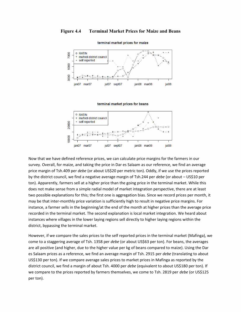
Figure 4.4 Terminal Market Prices for Maize and Beans

Now that we have defined reference prices, we can calculate price margins for the farmers in oursurvey. Overall, for maize, and taking the price in Dar es Salaam as our reference, we find an averageprice margin of Tsh.409 per debe (or about US$20 per metric ton). Oddly, if we use the prices reportedby the district council, we find a negative average margin of Tsh.244 per debe (or about – US$10 perton). Apparently, farmers sell at a higher price than the going price in the terminal market. While thisdoes not make sense from a simple radial model of market integration perspective, there are at leasttwo possible explanations for this; the first one is aggregation bias. Since we record prices per month, itmay be that inter-monthly price variation is sufficiently high to result in negative price margins. Forinstance, a farmer sells in the beginning/at the end of the month at higher prices than the average pricerecorded in the terminal market. The second explanation is local market integration. We heard aboutinstances where villages in the lower laying regions sell directly to higher laying regions within thedistrict, bypassing the terminal market.

However, if we compare the sales prices to the self reported prices in the terminal market (Mafinga), wecome to a staggering average of Tsh. 1358 per debe (or about US$63 per ton). For beans, the averagesare all positive (and higher, due to the higher value per kg of beans compared to maize). Using the Dares Salaam prices as a reference, we find an average margin of Tsh. 2915 per debe (translating to aboutUS$130 per ton). If we compare average sales prices to market prices in Mafinga as reported by thedistrict council, we find a margin of about Tsh. 4000 per debe (equivalent to about US$180 per ton). Ifwe compare to the prices reported by farmers themselves, we come to Tsh. 2819 per debe (or US$125per ton).

All the above is also summarized in the following kernel density estimates in Figure 4.5. The red curve isthe density plot for the distribution of the farm gate – Mafinga prices margin. The black curve representsthe farm gate – Dar es Salaam margin and the blue line represents the margin between the farm gateprices and the price in Mafinga as reported by the farmers themselves.

Figure 4.5 Kernel Density Estimates of Price Margins (US$/ton) for Maize and Beans

In sum, our estimates of price margins between farm gate prices and prices in the main regional market(Mafinga) show a high variance. For maize, it ranges from a negative margin to about Tsh.1358 per debe(US$63 per ton). For beans, we find average margins range between Tsh.2819 and Tsh.4000 per debe(between US$125 and US$180 per ton), depending on what reference prices are used.

4.3 Estimates of transaction costs at the regional level

In this part, we explain how, based on the theory of arbitrage, one can develop a dynamic model of pricebehaviour that gives an estimate of the transaction cost between two markets for a single,homogeneous commodity15. We start by briefly explaining the underlying idea and the empiricalstrategy. We then apply this model to time series data of maize prices of all possible combinations of 19markets, obtained from the Ministry of Industry, Trade and Marketing. The aim of this part is to get afirst sense of the transaction costs involved in regional trade.

If markets are connected through trade, economic theory predicts that prices of a single homogenousgood in those two markets will be related. The idea derives from the law of one price. It may be bestexplained by starting from an extreme situation where two spatially separated markets are completelyautarchic. In this case, the price of a commodity will be determined by local demand and local supply.Thus, there will be an equilibrium quantity and equilibrium price in market A and an equilibriumquantity and price in market B. A shift in local demand or local supply in one market will have no effecton the price of this commodity in the other market.

This changes if we allow for trade between market A and market B. If trade becomes possible, rationaleconomic agents will start exploiting spatial price differences. Suppose local demand and supplyconditions in market A are such that the price in this market for the commodity is lower than in marketB. This will prompt traders to buy the commodity in market A, ship it to market B and sell it there at thegoing (i.e. higher) price. The trader makes a per unit profit of the price difference.

What are the consequences of such arbitrage? More and more traders will enter the market (under theassumption of free market entry) as long as profit margins persist. But the increased demand for thecommodity in market A will increase the equilibrium price (assuming supply remains unchanged). At thesame time, the increased supply of the commodity in market B will, with unchanged demand, lower theprice in this market. In other words, the price difference between the commodities in the two markets

will diminish over time. Defining tm as the (absolute) price difference between market A and market B,

we get that:

15 Barrett (1996) makes a difference between three levels of market integration studies: Level I studies rely only onprice data of a single homogeneous good, recorded over time in spatially separated markets. Level II studies addinformation of flows of goods to this, while level III studies supplement both types of information with data ontransaction costs. While level II and III studies clearly allow for more precise estimates of the transaction cost, theyalso are much more data intensive. These days, price series data on different markets are routinely recorded bymarket authorities in key markets. Trade flows, on the other hand, are much more difficult to monitor thanprevailing prices. The same holds for the data on the transaction cost. This is defined as the cost of shipping goodsfrom one location to another location. While one could think this would be neatly approximated by recording theprices of fuel over time, it has to be noted that transaction costs entail much more than physical transport. Forexample, one would also need the cost of insuring the goods, the price of credit needed for the operation, etc. Webelieve the volume of price data in terms of observations can make up for the additions in terms of information inlevel II and III studies, provided we use the right econometric tools to exploit the information hidden in thedynamics of these price series.

ttt mm 1

Where t is a white noise error term and is to be estimated. Note that this is in fact a simple AR(1)

model. If markets are connected through trade and prices move towards each other over time, will

be estimated strictly negative16.

But prices will not be moving towards each other indefinitely. Indeed, rational arbitrageurs will onlytrade when they can make profit, that is, as long as the price difference exceeds the cost of moving thegoods between the two locations. As such, prices will move towards each other up to the point wherethe price difference is equal to the transaction cost between the two locations. Once the pricedifference becomes smaller then the transaction cost, the price of the commodity in each market will bedetermined by local supply and demand again, and these prices will move independently from eachother. This can be modelled by introducing thresholds into the AR model:

TmTmT

mTif

m

mm

t

t

t

tt

t

tt

t

1

1

1

1

1

Where T is the transaction cost. This model belongs to the class of piecewise linear regressions. To keepthings simple, we will assume symmetry. In other words, we will assume that the transaction cost ofshipping goods from A to B is the same as shipping from B to A. We will also assume that the speed atwhich prices converge over time is the same regardless of the direction of trade. A final assumption wemake is that the average transaction cost remains equal over time17. Figure 4.6 represents the functionwe estimate.

16 The β is called the adjustment speed. It indicates how fast the price margin reduces to zero over time (expressed asa percentage of the initial deviation). It forms the basis for the calculation of half-lives, which gives the time it takesfor a deviation in the margin from zero to return to half the value of the initial deviation.17 Strictly speaking, all these assumptions can be relaxed. It is possible to allow for different transaction costs and/oradjustment speed depending on the direction of trade (for instance, if one market is in the highlands, one may wantto take into account that it takes more fuel to get up the mountain than to get down). One just needs to specify anadditional regime. Van Campenhout (2007) also illustrates how to make the transaction cost a linear function oftime. However, relaxing the model has a price, either in a reduction of the observations in each regime or inincreased computation time as the algorithm needs to search over more dimensions. Our judgment is that thesymmetric transaction cost and adjustment speed outweigh the loss in precision due to the reduction of observationsin each regime. We also judged that our deflation methods would be sufficient to render an overall averagetransaction cost representative.

Figure 4.6 A piecewise linear regression model to estimate transaction costs

When one assumes symmetry, this piecewise linear regression has two regimes: one inside the bandformed by the transaction costs, and one outside (above the transaction cost or below the negative ofthe transaction cost). The theory predicts that when the price difference falls within the band formed bythe transaction cost, prices move independently. We can exploit this theoretical prediction to improveidentification of the transaction cost and the adjustment speed. We do this by imposing an adjustmentof zero inside the band formed by the transaction cost (which is equivalent to modelling the pricedifference as a random walk in this regime). The thresholds are identified using a grid search procedure.For more information and extensions to this model, as well as a discussion of alternative models, seeVan Campenhout (2007).

Inflation may be a concern, as we estimate transaction costs on the basis of time series data that coverroughly five years. However, one has to keep in mind that we model the price difference between twomarkets, and so one could argue that arbitrage conditions should hold for nominal price if the samedeflator is used. Unfortunately, the story does not end here. As transaction costs and adjustment speedsare identified by exploiting the dynamics of this price difference, inflation will affect our estimates18.

18 Consider the following simple example. There are two markets [A,B] and two points in time [0,1]. Suppose theprice of maize in market A at time 0 is 100, while in market B at time 0 it is 120. Hence the price margin at time 0 is20. Suppose now that at time 1, the price in market A is still 100, but the price in market B has reduced to 110. So, attime 1, the price margin has reduced to 10. The change in the price margin is thus -10. Suppose now that there is acommon inflation of 10 percent. Starting from the same situation, the price at time 1 in market A will now be 110.The price in market B at time 1 will 110(1+0.1)=121. Hence, the price margin will have decreased from 20 at time 0to 11 at time 1, which gives a change in the price margin of -9. Hence, the existence of common inflation in this casecreates a downward bias to the estimate of the adjustment speed due to the fact that the price difference gets inflatedas well.

(p1-p2) at t-1

So, recognizing we need to account for inflation somehow, the question comes up of what deflator touse. To get an accurate estimate of transaction costs through time series methods, it is advised to workwith time series of a reasonable frequency. For instance, if one expects arbitrage to take place in amatter of weeks, working with monthly price averages may severely bias the results (Taylor, 2001). Thisis why we work with weekly price series data. However, it is difficult to find an accepted deflator that isavailable at such a high frequency for prices in Tanzania. One way out would be to interpolate aconsumer price index at a lower frequency (eg. monthly) to a lower frequency (weekly). However, thismay reintroduce the aggregation bias reported in Taylor (2001). The alternative we use here is to takeout common inflation. More specifically, we remove average price changes from individual pricechanges before doing the analysis.

We will now apply this model to time series data of maize prices of 19 regional markets, obtained fromthe Ministry of Industry, Trade and Marketing . As an illustration, we plotted the series for three marketsin Figure 4.7. We estimate the above model for each possible bivariate market combination19. However,for some of the market pairs, an arbitrage connection is unlikely (for instance between say Bukoba andSumbawanga). The results of the 171 possible bivariate combinations are reported in Table A7 in theappendix. We will take subsets of these results to estimate transaction costs and measures of marketintegration.

19 In fact, the analysis assumes cointegration of price series. In other words, it assumes markets are connectedthrough arbitrage. The underlying theory views market integration not as a binary state (integrated or not) but ratheras a matter of degree (some markets are better integrated in the market system than others). As can be seen from thethree price series in Figure 4.7, prices are moving together in the long run. We agree we should test this formally forall market pairs on beforehand. But we are confident all price series will be cointegrated, even if we impose a (0, 1)cointegration vector (as implicit in our analysis, as we work with price difference). As our interest lies in the degreeof market integration (the transaction costs and the adjustment speed) we decided to leave this step out of theanalysis.

Figure 4.7 Time series data for prices of maize in three markets

We found that, over all possible combinations, the mean estimated transaction cost is about US$63 perton maize. The minimum transaction cost was found between Babati and Mbeya. It is only US$17 perton. Given the locations of these two cities, it is unlikely that there is a direct link between these twomarkets. However, the second lowest total transaction cost is found between two places that do trade:Arusha and Moshi. The estimated transaction cost here is as low as US$23 per ton. This should not comeas a surprise, as these towns are very close to each other and are connected by both a tarred road and arailway (see map in Appendix). The maximum transaction costs are found between Mwanza andSumbawanga and Mtwara and Sumbawanga. Here we estimate transaction costs of over US$112 perton of maize. This is also according to our expectations, as Sumbawanga is tucked away in the southwest of Tanzania behind Lake Rukwa. It is only accessible through Mbeya and the road is notoriouslybad. Mwanza is Tanzania's second largest city and located in the north on the shores of Lake Victoria.Mtwara is located at the coast all the way to the South. There is no tarred road connection.

However, as said above, some of these cities may not trade with each other. We see that those that arelikely to trade have generally higher adjustment speed. Hence, somewhat arbitrary, we select all marketpairs with an adjustment speed smaller than -0.2 and proceed with these trade routes from here. Wenow find that the average transaction cost is about US$50 per ton of maize, and the maximum is foundto be between Songea and Tabora (US$93 per ton).

We also measured the distance between the different regional markets. This allows us to expresstransaction costs per ton of maize per unit of distance. If we then average over all market pairs, we findan estimate of about US$100 per ton per 1000km (median US$91, mean US$104). The largesttransaction cost per unit of distance was US$365.90 per ton and was recorded between Lindi andMtwara, while the second largest transaction cost was recorded between Moshi and Arusha. Note that

these markets with highest per distance transaction cost are the ones that are very close to each other.The market pairs with the lowest per distance transaction costs, on the other hand, are all markets thatare relatively far from each other. For instance, the trade routes between Singida, Bukoba andShinyanga on the one end and Dar es Salaam on the other end all have transaction costs of less thanUS$40 per ton per 1000 km. This suggests significant fixed costs in maize trade20.

Even though we excluded market pairs that are unlikely to trade, the above estimates include marketsthat are connected through other towns. As such, it may be that maize moves into a town from twodifferent locations, and prices between these two locations are very similar (say lower than in thecentral market). While this would result in a low estimated transaction cost between the two supplymarkets, this would not reflect the real transaction cost between these two supply markets. It would bemore careful to look only at market pairs that are directly related to each other by road or railway andto not pass through other markets. If we confine ourselves to markets that are directly connected by aroad, we find mean transaction costs increase to about US$150 per ton per 1000km. The smallest cost isnow between Dar es Salaam and Moshi, and the largest cost is between Lindi and Mtwara. Since theseare, according to our judgement, the most accurate estimates, we reproduce them in Table 4.4 below.

20 The Pearson correlation coefficient between distance (km) and estimated transaction cost (US$) per 1000 km is -0.70 (p=0.00).

Table 4.4 Estimated transaction cost (US/ton per 1000 km)

DISTANCE ADJ HL TARRED US_1000KM

Arusha Moshi 80 -0.378 1.459 yes 296.4363Arusha Musoma 509 -0.228 2.675 no 91.40015Babati Singida 166 -0.229 2.661 no 252.2054Bukoba Kigoma 557 -0.209 2.949 no 102.0586Bukoba Shinyanga 503 -0.206 3.006 no 108.6183Bukoba Tabora 594 -0.531 0.915 no 120.6158Dar es Salaam Morogoro 194 -0.408 1.324 yes 169.8025Dar es Salaam Moshi 566 -0.309 1.874 yes 73.99889Dar es Salaam Tanga 356 -0.322 1.782 yes 86.82991Iringa Mbeya 337 -0.244 2.482 yes 112.1572Kigoma Tabora 415 -0.607 0.742 no 118.931Lindi Mtwara 106 -0.388 1.41 yes 365.9481Mbeya Songea 422 -0.228 2.673 yes 77.79472Mbeya Sumbawanga 374 -0.304 1.916 no 98.12776Mbeya Tabora 565 -0.409 1.318 no 130.9199Moshi Tanga 356 -0.236 2.575 yes 131.1185Musoma Mwanza 223 -0.25 2.412 yes 155.2364Mwanza Shinyanga 147 -0.33 1.732 yes 230.3228Shinyanga Singida 297 -0.261 2.291 no 131.5386Shinyanga Tabora 194 -0.752 0.497 no 176.8386Singida Tabora 332 -0.654 0.653 no 141.1694

We can use the transaction cost estimates between the market pairs to see which markets are betterintegrated with all others and which are worse integrated. This is done by simply taking the (average ofthe) estimated transaction cost per kilometre with (all) other market(s). The results are presented in 0.We coloured each region depending on the score obtained for the central market in each region. Whitecoloured regions mean that these regional markets have relatively low transaction costs per ton per1000km, while darker (black) relatively higher costs.

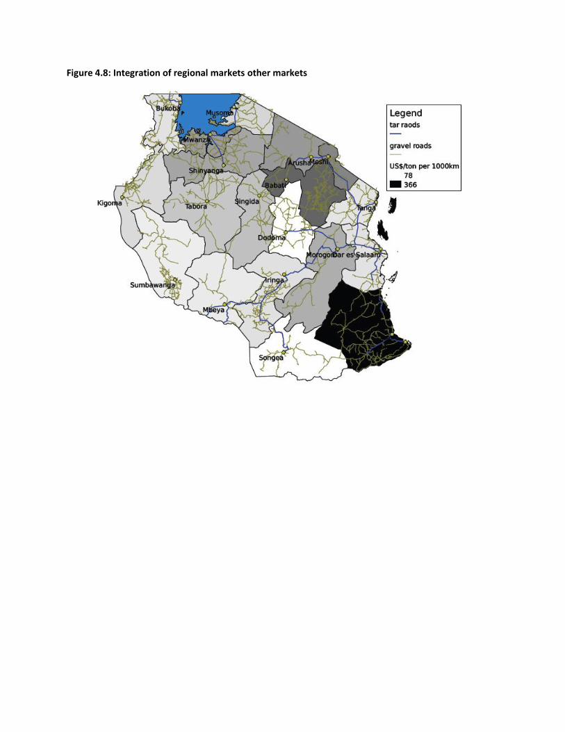
Figure 4.8: Integration of regional markets other markets

5 Conclusion, Recommendations and Ways Forward

The objective of this study was to come up with an estimate of transaction costs for agricultural andnon-agricultural products in Tanzania. Although our final estimates are based on the prices ofagricultural products due to lack data on non-agricultural products, we feel prices of non-agriculturalproducts are likely to be affected by similar transport costs.

In our review of literature, we have seen that since Tanzania covers a massive land area, thisnecessitates having in place an infrastructure or road and rail network that ensures that perishableproducts in the agriculture sector are transported efficiently. However, the reality is that Tanzania’stransport network is poor, and studies have documented spoilage of agricultural goods. Anotherconsequence of the poor transport system is that the wholesale-farm gate marketing margins ofagricultural goods are affected, as well as competitiveness of agricultural products. Where transactioncosts are high, they are translated into higher prices of retail crops and/or lower farm-gate prices forfarmers. The marketing margins differ with distance: terminal markets that are close to where theproducts are grown have lower marketing margins than terminal markets that are far from the source ofthe agricultural products. In terms of competition, high transport costs prevent farmers from securingbetter prices for the products as they are limited to selling to traders that come to them. High transportcosts do not just affect internal trade; they also affect Tanzania’s competitiveness in the export market.

The findings of our study on the effect of transaction costs are based on information coming from threesources. These are from the perspective of traders within Iringa, microeconomic data on farmers inIringa where data on prices was from three sources, and time series data from regional centres inTanzania. The findings from these studies are reported in different measures.

Traders report that transaction costs at the local level are about 10 percent of the farm gate price. Thisis equivalent to about Tsh.360 to Tsh.430 per debe (about 13US$ per ton to 15.5US$ per ton). Note thatat this level, we do not control for distance. Price margins based on farmers’ quoted prices are lessprecise. They range from a negative market price margin to as much as Tsh.1358 per debe (63US$ perton). At the regional level, we find an average transaction cost of about US$100 per ton per 1000km. Ifwe only consider only markets that are directly connected, this figure goes up to about about US$150per ton per 1000km. This confirms the estimates at the regional level, since these villages are on averageabout 100 km away from the terminal market (Mafinga).

Apart from the above estimates, we also observed some other interesting features. First, we weresurprised to find low levels of market participation in the villages studied. Second, we found thatalthough farmers do sell substantial amounts of maize and beans, this happens all at once, rather thandifferent sales of smaller amounts. This is strange in view of the substantial interpersonal movements ofprices. This may indicate that farmers have little choice in when to sell. For instance, they may needimmediate money, or they are visited only once by a trader. A third interesting finding was that, at aregional level, short transport routes were found to be more expensive than longer transport routes (ifexpressed per measure of distance). This may suggest substantial fixed costs in regional trade.

One interesting extension to this research would be to look at non-agricultural products. In addition, itwould be interesting to look at the prices and margins of a product that is not locally produced, butimported at one point (e.g., the harbour of Dar es Salaam). In this case, with no domestic production,the spatial price differences reflect only transaction costs and differences in local market demand; thereare no differences in supply that would complicate the analysis. Although the threshold autoregressivemodels presented in Section 4.3 should take care of these problems, it is always useful to havesomething to compare with. The above should in principle be possible, as the data are available. TheMinistry of Industry, Trade and Marketing collects price series data on several products. But also mobilephone companies disseminate price information these days.

In addition to this, it would be really interesting to take the regional price analysis to a local level. Thatis, during a specific period of time, record prices within the villages that were used in the trader survey(and the terminal markets of Mafinga and Makambako). This would allow us to see if the extent ofmarket integration (with associated speed of adjustment and transaction costs) that has been found ona regional level carries over to the local level. This should not be so difficult or costly. It would involvesome enumerators keeping track of a range of prices. If we take the time interval sufficiently high (e.g.,daily) it would not take too long before we can come up with some initial estimates.

One of the interesting findings was, as mentioned above, the fact that farmers seem to sell substantialamounts of maize. However, instead of taking advantage of price differences over the agricultural cycle,farmers usually sell everything at once, often immediately after the harvest. There may be differentreasons for this, like a lack of competition in the traders market. It has also been argued that missingcredit market may be the root cause of this behaviour (Stephens and Barrett, 2010). It would beinteresting to do some more research on this.

6 REFERENCES

AICD (Africa Infrastructure Country Diagnostic), (2010), “Tanzania’s Infrastructure: A ContinentalPerspective”, Country Report.

Agra CEAS Consulting, (2007), The Gap Between Producer Prices and the Prices Paid by the ConsumerStudy”, Study requested by the European Parliament's Committee On Agriculture and RuralDevelopment.

Bank of Tanzania, (2009), Economic Bulletin for the Quarter Ending March, 2009, Vol. XLI No. 1.

Barrett, C.B., (1996),” Market Analysis Methods: Are Our Enriched Toolkits Well Suited to EnlivenedMarkets?”, American Journal of Agricultural Economics,78: 825-829.

Carcani, D., (2010), “Deja Vu? World Food Price Hikes Raise Concerns”, Diplomatic Courier news articles,www.diplomaticourier.org.

D'Exelle, B, Lecoutere, E. and Van Campenhout, B., (2010), “Social Status and Bargaining whenResources are Scarce: Evidence from a Field Lab Experiment”, CBESS Discussion Paper 10-09, Norwich:University of East Anglia.

Eichengreen, B., (1994), “The Contributions of Robert W. Fogel to Economics and Economic History”, TheScandinavian Journal of Economics, Vol. 96 (2): 167-179.

Eskola, E., (2005), “Agricultural Marketing and Supply Chain Management in Tanzania: A Case Study”, AnESRF Study on Globalisation and East Africa Economies.

Hine, J. L. and Ellis, S. D., (2001), “Agricultural Marketing and Access to Transport Services”, RuralTransport Knowledge Base, Rural Travel and Transport Program 2001.

Kähkönen, S and Leathers, H., (1999), “Transaction Costs Analysis of Maize and Cotton Marketing inZambia and Tanzania”, SD Publication Series, Technical Paper No. 105.

Kweka, J., (2006), “Trade and Transport Costs in Tanzania”, CREDIT Research Paper 06/10, School ofEconomics, University of Nottingham.

Lecoutere, E., D’Exelle, B. and Van Campenhout, B., (2010), “Who Engages in Water Scarcity Conflicts? AField Experiment with Irrigators in Semi-arid Africa”, MICROCON Research Working Paper 31, Brighton:MICROCON.

Mduma, J.K., and Kipsat, M., (2009), “Asymmetric Price Transmission in Tanzania’s Maize MarketingSystem: Application of Exceedence Analysis”, Tanzania Economic Trends, Vol. 20 (1): 81-90.

Morrissey, O., and Leyaro, V., (2007), “Distortions to Agricultural Incentives in Tanzania”, AgriculturalDistortions Working Paper 52, CREDIT, University of Nottingham.

National Bureau of Statistic (NBS), (2009), Household Budget Survey 2007, Dar es Salaam.

National Bureau of Statistics (NBS), (2007), Revised National Accounts Estimates for Tanzania Mainland,Base Year, 2001, Dar es Salaam.

Okoh, R., and Egbon, P.C., (2005), “The Integration of Nigeria's Rural and Urban Foodstuffs Markets”,AERC Research Paper 151.

Rapsomanikis, G., and Karfakis, P., (2007), “Margins Across Time and Space: Threshold Cointegration andSpatial Pricing Applications to Commodity Markets in Tanzania”, Paper presented in the Workshop onStaple Food Trade and Market Policy Option for Promoting Development in Eastern and Southern Africa,Rome.

Rapsomanikis, G., Hallam, D., and Conforti, P., (2003), “Market Integration and Price Transmission inSelected Food and Cash Crop Markets of Developing Countries: Review and Applications”, in CommodityMarket Review 2003-2004, FAO.

Stephens, E and Barrett, C., (2010), Incomplete Credit Markets and Commodity Market Behaviour”,Journal of Agricultural Economics, forthcoming.

Taylor, A. M., (2001), Potential Pitfalls for the Purchasing-Power-Parity Puzzle? Sampling andSpecification Biases in Mean-Reversion Tests of the Law of One Price," Econometrica, 69(2): 473-9.

Van Campenhout, B., 2007. "Modelling trends in food market integration: Method and an application toTanzanian maize markets," Food Policy, Elsevier, vol. 32(1), pages 112-127

Von Braun, J., Hazell, P., Hoddinott, J., and Babu, S (2003), “Achieving Long-Term Food Security InSouthern Africa: International Perspectives, Investment Strategies And Lessons”, Keynote paperprepared for the Southern Africa Regional Conference on "Agricultural Recovery, Trade and Long-termFood Security," March 26-27, 2003, Gaborone, Botswana.

World Bank, (2010), World Development Indicators CD-ROM.

7 Appendices

Table A1: Transport Indicators

LAND AREA(SQ.KM)

TOTAL ROAD networkper LAND area (%)*

ROADS, PAVED (%OF TOTAL ROADS)*

Algeria 2381740 4.5 69.5

Angola 1246700 4.1 10.4

Benin 110620 17.2 9.5

Botswana 566730 4.4 34.1

Burkina Faso 273600 33.8 4.2

Burundi 25680 52.2 8.8

Cameroon 465400 10.9 8.2

Cape Verde 4030 33.5 69.0

Chad 1259200 3.0 0.8

Comoros 1861 47.3 76.5

Congo, Dem. Rep. 2267050 6.8 1.8

Congo, Rep. 341500 4.4 7.3

Cote d'Ivoire 318000 20.5 8.9

Egypt, Arab Rep. 995450 7.9 79.5

Ethiopia 1000000 3.6 12.6

Gabon 257670 3.4 10.1

Gambia, The 10000 33.9 24.7

Ghana 227540 21.6 20.2

Guinea 245720 15.2 13.1

Guinea-Bissau 28120 12.3 27.9

Kenya 569140 11.2 13.1

Lesotho 30350 19.6 18.3

Liberia 96320 11.0 6.2

Libya 1759540 4.7 57.2

Madagascar 581540 8.6 11.6

Malawi 94080 16.4 45.0

Mali 1220190 1.4 15.1

Mauritania 1030700 0.9 22.8

Mauritius 2030 98.5 99.0

Morocco 446300 12.9 58.1

Mozambique 786380 3.9 18.7

Namibia 823290 6.6 12.8

Niger 1266700 1.3 23.0

Nigeria 910770 21.2 15.0

Rwanda 24670 52.7 13.7

Senegal 192530 7.3 29.3

Seychelles 460 99.6 96.0

Sierra Leone 71620 15.8 8.0

Somalia 627340 3.5 11.8

South Africa 1214470 29.9 18.8

Sudan 2376000 0.5 36.3

Swaziland 17200 19.9 30.0

Tanzania 885800 9.4 6.4

Togo 54390 13.8 31.6

Tunisia 155360 12.3 66.5

Uganda 197100 35.9 23.0

Zambia 743390 10.6 22.0

Zimbabwe 386850 25.1 19.0

Note: *Average for 2000-2007.Source: Authors’ calculations and World Bank (2010), World Development Indicators CD-ROM.

Table A2: Between City Price Differences of Maize

Wholesale prices (Tsh. per100kg bag)

IRINGA DODOMA

August 1994 6,800 6,250

August 1995 4,600 8,500

Producer prices (Tsh. per 90kgbag)

SENGEREMA NJOMBE MAFINGA MOINGA

June 1996 3,750 10,000 10,500 5,250

Retail prices, May 1996, (Tsh.per debe - 18kg)

MOROGORO DAR ES SALAAM NJOMBE IRINGA

May 1996 1,550 2,800 1,300 2,225

Source: Kähkönen and Leathers (1999).

Table A3: Estimates of Marketing Margins along the National Supply Chain

Local Traders/Brokers (rice at Ifakara) 10-20% per kilo

Regional traders in Mtwara 2-4% per kilo

Brokers of transport 10% of transport fee

Large-scale traders Tshs.20,000 per trip (regions)

Broker (green bananas at Ubungo) 7-11% per bunch

Broker (onions at Kariakoo) 4% per bag

Wholesaler (grain at Kariakoo) Tshs.10-15,000 daily

Whosaler (rice at Tandale) 8% per kilo

Retailer (potato at Kinondoni) 36% per kilo

Retailer (oranges at Tandale) 20-70% per orange

Retailer (banana at Ilala) 15% per basket

Tanzanian export agent (cashew nuts) 3% per kilo

Indian export agent (cashew nuts) 4-5% per kilo

Subagents for the exporter (cashew nuts) 1% per kilo

Source: Eskola (2005).

Table A4: Estimates of Transport Costs

KM. TSH. (PER10 TONS)

TSH./KM. TSH. (PERTON PERKM)

$ (PERTON PERKM*)

$ (PERTON PER100KM)

Dar es Salaam – Mwanza 1164 1,200,000 1030.9 103.1 0.09 9.13

Dar es Salaam – Iringa 501 200,000 399.2 39.9 0.04 3.54

Dar es Salaam – Mbeya 851 450,000 528.8 52.9 0.05 4.68

Dar es Salaam – Dodoma 479 250,000 521.9 52.2 0.05 4.62

Dar es Salaam – Mtwara 565 800,000 1415.9 141.6 0.13 12.54

Dar es Salaam – Singida 709 500,000 705.2 70.5 0.06 6.25

Dar es Salaam –Rukwa/Sumbawanga

1203 1,350,000 1122.2 112.2 0.10 9.94

Dar es Salaam – Lindi 562 600,000 1067.6 106.8 0.09 9.46

Dar es Salaam – Arusha 647 450,000 695.5 69.6 0.06 6.16

Dar es Salaam –Kilimanjaro/Moshi

562 300,000 533.8 53.4 0.05 4.73

Dar es Salaam – Morogoro 196 150,000 765.3 76.5 0.07 6.78

Dar es Salaam – Mara 1369 1,300,000 949.6 95.0 0.08 8.41

Dar es Salaam – Tanga 354 225,000 635.6 63.6 0.06 5.63

Dar es Salaam – Manyara 440 500,000 1136.4 113.6 0.10 10.07

Dar es Salaam – Ruvuma/Songea 992 700,000 705.6 70.6 0.06 6.25

Dar es Salaam – Kigoma 1442 1,200,000 832.2 83.2 0.07 7.37

Dar es Salaam – Tabora 1039 800,000 769.9 77.0 0.07 6.82

Dar es Salaam – Pwani 68 80,000 1176.5 117.7 0.10 10.42

Dar es Salaam – Kagera 1425 1,600,000 1122.8 112.3 0.10 9.95

Dar es Salaam – Shinyanga 1001 800,000 799.2 79.9 0.07 7.08

*Exchange rate use is the annual average in 2005 when the study was done, which was Tsh.1129/$US.Source: Eskola (2005).

Table A5: Estimates of Domestic Freight Rates

1998 1999 2000 2001 2002 Average

Livestock 0.071 0.096 0.102 0.097 0.110 0.082

Food Products 0.027 0.028 0.029 0.036 0.036 0.028

Coffee, tea, cotton & sugar 0.058 0.069 0.073 0.077 0.083 0.064

Fish Products 0.000 0.000 0.000 0.000 0.000 0.000

Fish Products 0.000 0.000 0.000 0.000 0.000 0.000

Beverages and Tobacco 0.092 0.099 0.105 0.115 0.121 0.095

Mineral Products 0.041 0.060 0.064 0.069 0.073 0.054

Chemical Products 0.055 0.081 0.087 0.095 0.100 0.073

Forestry Products 0.025 0.027 0.028 0.029 0.031 0.026

Building Materials 0.071 0.082 0.090 0.181 0.150 0.100

Textile and clothing and leather 0.023 0.008 0.008 0.009 0.010 0.011

Metal products and machinery 0.032 0.044 0.047 0.044 0.050 0.039

Transport equipment 0.031 0.043 0.045 0.043 0.049 0.038

Other manufactures 0.059 0.060 0.086 0.103 0.104 0.072

Average 0.042 0.050 0.055 0.065 0.066 0.049

Source: Kweka (2006).

Table A6: Estimates of Marketing Margins (%)

Early 90s Late 90s 2000s

Cash Crops 25 10 10

Food Crops 10-20

Other food crops 20-30

Staple foods <5 <5 <5

Source: Morrissey and Leyaro (2007).

Table A7: Estimated Transaction Costs and Adjustment Speed

Distance (km) thres_res Cost/km adj_res hl_res1 Arusha_Babati 166 4925 29.669 -0.276 2.1462 Arusha_Bukoba 1025 7187 7.012 -0.194 3.2123 Arusha_Dar es Salaam 645 3702 5.74 -0.433 1.2234 Arusha_Iringa 907 6951 7.664 -0.126 5.1375 Arusha_Kigoma 1074 6927 6.45 -0.182 3.4456 Arusha_Lindi 1103 8032 7.282 -0.161 3.9547 Arusha_Mbeya 1233 8556 6.939 -0.077 8.7018 Arusha_Morogoro 594 2782 4.684 -0.296 1.9759 Arusha_Moshi 80 2745 34.313 -0.378 1.45910 Arusha_Mtwara 1207 7580 6.28 -0.192 3.24911 Arusha_Musoma 509 5385 10.58 -0.228 2.67512 Arusha_Mwanza 615 5811 9.449 -0.116 5.601

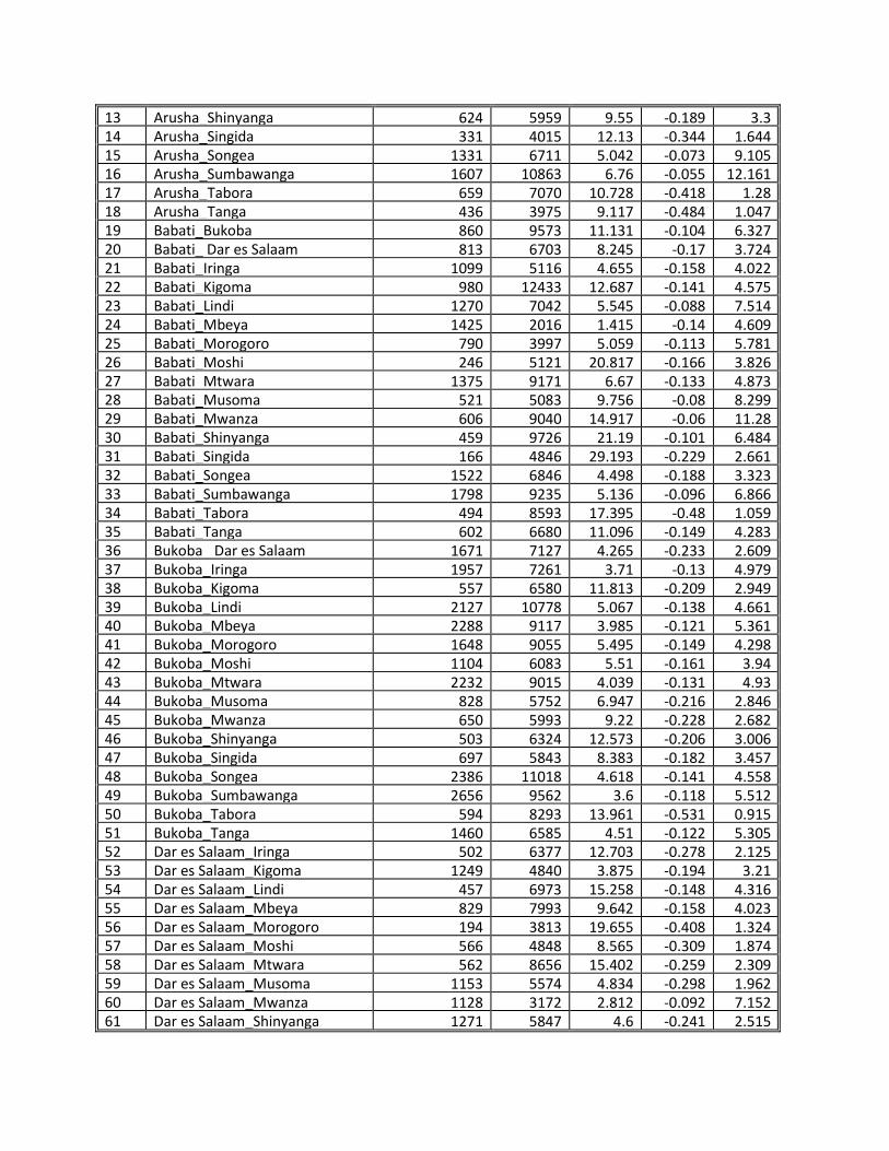
13 Arusha_Shinyanga 624 5959 9.55 -0.189 3.314 Arusha_Singida 331 4015 12.13 -0.344 1.64415 Arusha_Songea 1331 6711 5.042 -0.073 9.10516 Arusha_Sumbawanga 1607 10863 6.76 -0.055 12.16117 Arusha_Tabora 659 7070 10.728 -0.418 1.2818 Arusha_Tanga 436 3975 9.117 -0.484 1.04719 Babati_Bukoba 860 9573 11.131 -0.104 6.32720 Babati_ Dar es Salaam 813 6703 8.245 -0.17 3.72421 Babati_Iringa 1099 5116 4.655 -0.158 4.02222 Babati_Kigoma 980 12433 12.687 -0.141 4.57523 Babati_Lindi 1270 7042 5.545 -0.088 7.51424 Babati_Mbeya 1425 2016 1.415 -0.14 4.60925 Babati_Morogoro 790 3997 5.059 -0.113 5.78126 Babati_Moshi 246 5121 20.817 -0.166 3.82627 Babati_Mtwara 1375 9171 6.67 -0.133 4.87328 Babati_Musoma 521 5083 9.756 -0.08 8.29929 Babati_Mwanza 606 9040 14.917 -0.06 11.2830 Babati_Shinyanga 459 9726 21.19 -0.101 6.48431 Babati_Singida 166 4846 29.193 -0.229 2.66132 Babati_Songea 1522 6846 4.498 -0.188 3.32333 Babati_Sumbawanga 1798 9235 5.136 -0.096 6.86634 Babati_Tabora 494 8593 17.395 -0.48 1.05935 Babati_Tanga 602 6680 11.096 -0.149 4.28336 Bukoba_ Dar es Salaam 1671 7127 4.265 -0.233 2.60937 Bukoba_Iringa 1957 7261 3.71 -0.13 4.97938 Bukoba_Kigoma 557 6580 11.813 -0.209 2.94939 Bukoba_Lindi 2127 10778 5.067 -0.138 4.66140 Bukoba_Mbeya 2288 9117 3.985 -0.121 5.36141 Bukoba_Morogoro 1648 9055 5.495 -0.149 4.29842 Bukoba_Moshi 1104 6083 5.51 -0.161 3.9443 Bukoba_Mtwara 2232 9015 4.039 -0.131 4.9344 Bukoba_Musoma 828 5752 6.947 -0.216 2.84645 Bukoba_Mwanza 650 5993 9.22 -0.228 2.68246 Bukoba_Shinyanga 503 6324 12.573 -0.206 3.00647 Bukoba_Singida 697 5843 8.383 -0.182 3.45748 Bukoba_Songea 2386 11018 4.618 -0.141 4.55849 Bukoba_Sumbawanga 2656 9562 3.6 -0.118 5.51250 Bukoba_Tabora 594 8293 13.961 -0.531 0.91551 Bukoba_Tanga 1460 6585 4.51 -0.122 5.30552 Dar es Salaam_Iringa 502 6377 12.703 -0.278 2.12553 Dar es Salaam_Kigoma 1249 4840 3.875 -0.194 3.2154 Dar es Salaam_Lindi 457 6973 15.258 -0.148 4.31655 Dar es Salaam_Mbeya 829 7993 9.642 -0.158 4.02356 Dar es Salaam_Morogoro 194 3813 19.655 -0.408 1.32457 Dar es Salaam_Moshi 566 4848 8.565 -0.309 1.87458 Dar es Salaam_Mtwara 562 8656 15.402 -0.259 2.30959 Dar es Salaam_Musoma 1153 5574 4.834 -0.298 1.96260 Dar es Salaam_Mwanza 1128 3172 2.812 -0.092 7.15261 Dar es Salaam_Shinyanga 1271 5847 4.6 -0.241 2.515

62 Dar es Salaam_Singida 978 3904 3.992 -0.253 2.37663 Dar es Salaam_Songea 927 9212 9.937 -0.145 4.41864 Dar es Salaam_Sumbawan 1203 10920 9.077 -0.118 5.50765 Dar es Salaam_Tabora 835 7093 8.495 -0.478 1.06566 Dar es Salaam_Tanga 356 3578 10.051 -0.322 1.78267 Iringa_Kigoma 1054 10628 10.083 -0.142 4.53668 Iringa_Lindi 959 11507 11.999 -0.161 3.96269 Iringa_Mbeya 337 4375 12.982 -0.244 2.48270 Iringa_Morogoro 313 7000 22.364 -0.159 4.00271 Iringa_Moshi 854 9372 10.974 -0.12 5.43172 Iringa_Mtwara 1065 10734 10.079 -0.13 4.99673 Iringa_Musoma 1442 8508 5.9 -0.132 4.88374 Iringa_Mwanza 1549 9967 6.434 -0.089 7.45575 Iringa_Shinyanga 1558 5938 3.811 -0.075 8.90176 Iringa_Singida 1265 5927 4.685 -0.213 2.88877 Iringa_Songea 435 3042 6.993 -0.186 3.36578 Iringa_Sumbawanga 711 7336 10.318 -0.209 2.95579 Iringa_Tabora 641 8320 12.98 -0.419 1.27780 Iringa_Tanga 641 7881 12.295 -0.212 2.90881 Kigoma_Lindi 1706 5462 3.202 -0.149 4.30182 Kigoma_Mbeya 975 10269 10.532 -0.142 4.51583 Kigoma_Morogoro 1060 7072 6.672 -0.178 3.54184 Kigoma_Moshi 1154 5973 5.176 -0.146 4.37885 Kigoma_Mtwara 1811 7195 3.973 -0.2 3.10286 Kigoma_Musoma 933 4800 5.145 -0.207 2.98187 Kigoma_Mwanza 756 4294 5.68 -0.261 2.29288 Kigoma_Shinyanga 609 4746 7.793 -0.41 1.31589 Kigoma_Singida 747 4477 5.993 -0.19 3.28790 Kigoma_Songea 1395 12641 9.062 -0.14 4.5891 Kigoma_Sumbawanga 1005 12301 12.24 -0.098 6.73692 Kigoma_Tabora 415 5713 13.766 -0.607 0.74293 Kigoma_Tanga 1301 7182 5.52 -0.137 4.70994 Lindi_Mbeya 1284 10979 8.551 -0.155 4.11295 Lindi_Morogoro 648 6151 9.492 -0.181 3.46996 Lindi_Moshi 1020 9604 9.416 -0.11 5.94597 Lindi_Mtwara 106 4490 42.358 -0.388 1.4198 Lindi_Musoma 1607 4471 2.782 -0.071 9.46599 Lindi_Mwanza 1714 6035 3.521 -0.099 6.661100 Lindi_Shinyanga 1723 4291 2.49 -0.124 5.257101 Lindi_Singida 1432 7295 5.094 -0.145 4.42102 Lindi_Songea 1381 12730 9.218 -0.137 4.706103 Lindi_Sumbawanga 1607 10906 6.787 -0.124 5.217104 Lindi_Tabora 1290 8258 6.402 -0.443 1.186105 Lindi_Tanga 810 9099 11.233 -0.138 4.682106 Mbeya_Morogoro 640 8729 13.639 -0.108 6.048107 Mbeya_Moshi 1182 8043 6.805 -0.084 7.901108 Mbeya_Mtwara 1395 11149 7.992 -0.111 5.868109 Mbeya_Musoma 1083 8846 8.168 -0.106 6.161110 Mbeya_Mwanza 905 10320 11.403 -0.072 9.276

111 Mbeya_Shinyanga 759 9100 11.989 -0.118 5.503112 Mbeya_Singida 602 6573 10.919 -0.154 4.153113 Mbeya_Songea 422 3800 9.005 -0.228 2.673114 Mbeya_Sumbawanga 374 4248 11.358 -0.304 1.916115 Mbeya_Tabora 565 8562 15.154 -0.409 1.318116 Mbeya_Tanga 968 9687 10.007 -0.159 4.001117 Morogoro_Moshi 543 5398 9.941 -0.264 2.258118 Morogoro_Mtwara 756 5534 7.32 -0.175 3.6119 Morogoro_Musoma 1133 4689 4.139 -0.17 3.731120 Morogoro_Mwanza 1239 4406 3.556 -0.109 6.024121 Morogoro_Shinyanga 1248 6891 5.522 -0.181 3.476122 Morogoro_Singida 955 5449 5.706 -0.27 2.2123 Morogoro_Songea 737 10737 14.569 -0.117 5.579124 Morogoro_Sumbawanga 1023 7580 7.41 -0.054 12.57125 Morogoro_Tabora 646 7778 12.04 -0.382 1.44126 Morogoro_Tanga 333 3626 10.889 -0.409 1.319127 Moshi_Mtwara 1128 7395 6.556 -0.125 5.205128 Moshi_Musoma 589 2864 4.862 -0.21 2.936129 Moshi_Mwanza 695 6198 8.918 -0.125 5.191130 Moshi_Shinyanga 704 4736 6.727 -0.128 5.08131 Moshi_Singida 411 4454 10.837 -0.163 3.889132 Moshi_Songea 1278 8536 6.679 -0.086 7.721133 Moshi_Sumbawanga 1562 11938 7.643 -0.055 12.257134 Moshi_Tabora 962 7998 8.314 -0.447 1.17135 Moshi_Tanga 356 5403 15.177 -0.236 2.575136 Mtwara_Musoma 1712 4529 2.645 -0.087 7.586137 Mtwara_Mwanza 1821 5968 3.277 -0.108 6.036138 Mtwara_Shinyanga 1830 5069 2.77 -0.121 5.391139 Mtwara_Singida 1537 7997 5.203 -0.126 5.169140 Mtwara_Songea 1486 12124 8.159 -0.154 4.14141 Mtwara_Sumbawanga 1765 13182 7.469 -0.133 4.874142 Mtwara_Tabora 1394 8789 6.305 -0.386 1.42143 Mtwara_Tanga 915 8605 9.404 -0.211 2.927144 Musoma_Mwanza 223 4007 17.969 -0.25 2.412145 Musoma_Shinyanga 327 5403 16.523 -0.197 3.165146 Musoma_Singida 622 6278 10.093 -0.198 3.148147 Musoma_Songea 1865 9852 5.283 -0.078 8.547148 Musoma_Sumbawanga 2144 10725 5.002 -0.061 11.065149 Musoma_Tabora 518 7827 15.11 -0.455 1.142150 Musoma_Tanga 943 7123 7.554 -0.176 3.579151 Mwanza_Shinyanga 147 3919 26.66 -0.33 1.732152 Mwanza_Singida 444 5092 11.468 -0.121 5.394153 Mwanza_Songea 1973 12650 6.412 -0.067 10.035154 Mwanza_Sumbawanga 1772 13074 7.378 -0.055 12.335155 Mwanza_Tabora 341 6832 20.035 -0.501 0.996156 Mwanza_Tanga 1051 9556 9.092 -0.092 7.15157 Shinyanga_Singida 297 4522 15.226 -0.261 2.291158 Shinyanga_Songea 1982 11360 5.732 -0.101 6.499159 Shinyanga_Sumbawanga 2258 8207 3.635 -0.068 9.904

160 Shinyanga_Tabora 194 3971 20.469 -0.752 0.497161 Shinyanga_Tanga 1060 8774 8.277 -0.127 5.11162 Singida_Songea 1686 7922 4.699 -0.177 3.554163 Singida_Sumbawanga 927 7247 7.818 -0.111 5.864164 Singida_Tabora 332 5425 16.34 -0.654 0.653165 Singida_Tanga 766 5260 6.867 -0.315 1.831166 Songea_Sumbawanga 818 4874 5.958 -0.327 1.748167 Songea_Tabora 1073 10816 10.08 -0.27 2.199168 Songea_Tanga 1065 9170 8.61 -0.143 4.482169 Sumbawanga_Tabora 595 9809 16.486 -0.387 1.416170 Sumbawanga_Tanga 1342 9445 7.038 -0.069 9.667171 Tabora_Tanga 1095 8770 8.009 -0.378 1.46

Appendix 2Figure 1: Map of Tanzania's Road and Railway Network