PLASMID ISOLATION AND ANALYSIS Part II Plasmid Purification and Isolation
1
Estimating the rate of plasmid transfer with an adapted Luria–Delbrück fluctuation
analysis and a case study on the evolution of plasmid transfer rate
Olivia Kosterlitz1,2*, Clint Elg2,3, Ivana Bozic4, Eva M. Top2,3, Benjamin Kerr1,2*
1 Biology Department, University of Washington, Seattle, WA, USA.
2 BEACON Center for the Study of Evolution in Action, East Lansing, MI, USA.
3 Department of Biological Sciences and Institute for Bioinformatics and Evolutionary
Studies, University of Idaho, Moscow, ID, USA.
4 Department of Applied Mathematics, University of Washington, Seattle, WA, USA.
* e-mail: [email protected]; [email protected]
Author contributions
O.K. and B.K. conceived of the presented ideas. B.K. and I.B. developed the theory. O.K.
developed and performed the simulations. C.E. facilitated part of the simulations. O.K.
performed the experiments. O.K. and B.K. wrote the manuscript. E.M.T. and B.K.
supervised the project. All authors discussed the results and contributed to the final
manuscript.
.CC-BY-NC-ND 4.0 International licenseavailable under awas not certified by peer review) is the author/funder, who has granted bioRxiv a license to display the preprint in perpetuity. It is made
The copyright holder for this preprint (whichthis version posted June 7, 2021. ; https://doi.org/10.1101/2021.01.06.425583doi: bioRxiv preprint

2
Abstract 1
To increase our basic understanding of the ecology and evolution of conjugative 2
plasmids, we need a reliable estimate of their rate of transfer between bacterial cells. 3
Accurate estimates of plasmid transfer have remained elusive given biological and 4
experimental complexity. Current methods to measure transfer rate can be confounded 5
by many factors, such as differences in growth rates between plasmid-containing and 6
plasmid-free cells. However, one of the most problematic factors involves situations 7
where the transfer occurs between different strains or species and the rate that one type 8
of cell donates the plasmid is not equal to the rate at which the other cell type donates. 9
Asymmetry in these rates has the potential to bias transfer estimates, thereby limiting our 10
capabilities for measuring transfer within diverse microbial communities. We develop a 11
novel low-density method (“LDM”) for measuring transfer rate, inspired by the classic 12
fluctuation analysis of Luria and Delbrück. Our new approach embraces the stochasticity 13
of conjugation, which departs in important ways from the current deterministic population 14
dynamic methods. In addition, the LDM overcomes obstacles of traditional methods by 15
allowing different growth and transfer rates for each population within the assay. Using 16
stochastic simulations, we show that the LDM has high accuracy and precision for 17
estimation of transfer rates compared to other commonly used methods. Lastly, we 18
implement the LDM to estimate transfer on an ancestral and evolved plasmid-host pair, 19
in which plasmid-host co-evolution increased the persistence of an IncP-1 conjugative 20
plasmid in its Escherichia coli host. Our method revealed the increased persistence can 21
be at least partially explained by an increase in transfer rate after plasmid-host co-22
evolution. 23
24
Introduction 25
A fundamental rule of life and the basis of heredity involves the passage of genes 26
from parents to their offspring. Plasmids in bacteria can violate this rule of strict vertical 27
inheritance by shuttling DNA among neighboring, non-related bacteria through horizontal 28
gene transfer (HGT). Plasmids are independently replicating extrachromosomal DNA 29
molecules, and some encode for their own horizontal transfer, a process termed 30
conjugation. Bacteria containing such conjugative plasmids are governed by two modes 31
of inheritance: vertical and horizontal. In an abstract sense, conjugation in prokaryotes is 32
similar to the genetic recombination that occurs in sexually reproducing eukaryotes; 33
specifically, conjugation is a fundamental mechanism for producing new combinations of 34
.CC-BY-NC-ND 4.0 International licenseavailable under awas not certified by peer review) is the author/funder, who has granted bioRxiv a license to display the preprint in perpetuity. It is made
The copyright holder for this preprint (whichthis version posted June 7, 2021. ; https://doi.org/10.1101/2021.01.06.425583doi: bioRxiv preprint

3
genetic elements. Since conjugation facilitates gene flow across vast phylogenetic 35
distances, the expansive gene repertoire in the “accessory” genome is shared among 36
many microbial species1. While this complicates phylogenetic inference, it reinforces the 37
notion that conjugation has a central role in shaping the ecology and evolution of microbial 38
communities2,3. Notably, conjugative plasmids are commonly the vehicle for the spread 39
of antimicrobial resistance (AMR) genes and the emergence of multi-drug resistance 40
(MDR) in clinical pathogens4. While such plasmids may impose growth costs on their 41
bacterial hosts in the absence of antibiotics5, theoretical and experimental studies have 42
demonstrated how conjugation itself may be a critical process for the invasion and 43
maintenance of costly plasmids6,7,8. To model the spread of antibiotic resistance, improve 44
phylogenetic inference, and increase our understanding of the fundamental process of 45
conjugation and its impacts on the basic biology of bacteria, accurate measures of 46
conjugation are of the utmost importance. 47
The basic approach to measure conjugation involves mixing plasmid-containing 48
bacteria, called “donors”, with plasmid-free bacteria, called “recipients”. After donors and 49
recipients are incubated together for some period of time, which is hereafter denoted as 50
�̃�, the population is assessed for recipients that have received the plasmid from the donor; 51
these transformed recipients are called “transconjugants”. To describe conjugation the 52
earliest and some of the most widely used approaches measure the densities of donors, 53
recipients, and transconjugants after the incubation time �̃� (𝐷𝑡, 𝑅𝑡, and 𝑇𝑡, respectively) to 54
calculate various ratios (i.e., conjugation frequency or efficiency) including 𝑇𝑡/𝑅𝑡, 𝑇𝑡/𝐷�̃�, 55
𝑇𝑡/(𝐷𝑡 + 𝑅𝑡 + 𝑇�̃�)9, see Zhong et. al.10 and Huisman et. al.11 for a comprehensive 56
overview. These conjugation ratios are descriptive statistics and have been shown to vary 57
with initial densities (𝐷0 and 𝑅0) and incubation time (�̃�)10,11. While these statistics may be 58
useful for within study comparisons of the combined processes of conjugation and 59
transconjugant growth, they are not estimating the rate of conjugation events. To see this, 60
consider two plasmids, A and B, and assume both have the same conjugation rate, but 61
plasmid A results in a higher transconjugant growth rate. Assuming all other parameters 62
(e.g., donor growth, recipient growth, etc.) are the same and growth occurs during the 63
assay, all of the above ratios would be higher for A, even though its conjugation rate 64
doesn’t differ from plasmid B. Clearly, an estimate of the rate of conjugation itself is 65
desirable. 66
The conjugation rate (i.e., plasmid transfer rate) is the “gold-standard” 67
measurement to describe conjugation akin to measuring other fundamental rate 68
.CC-BY-NC-ND 4.0 International licenseavailable under awas not certified by peer review) is the author/funder, who has granted bioRxiv a license to display the preprint in perpetuity. It is made
The copyright holder for this preprint (whichthis version posted June 7, 2021. ; https://doi.org/10.1101/2021.01.06.425583doi: bioRxiv preprint

4
parameters, such as growth rate or mutation rate. Such metrics are useful for cross-69
literature comparison to understand basic microbial ecology and evolution12. There are 70
only a few widely used methods to measure conjugation rate, which all are derived from 71
the Levin et. al.13 mathematical model describing the change in density of donors, 72
recipients and transconjugants over time (given by dynamic variables 𝐷𝑡, 𝑅𝑡, and 𝑇𝑡, 73
respectively). In this model, each population type grows exponentially at the same growth 74
rate 𝜓. In addition, the transconjugant density increases as a result of conjugation events 75
both from donors to recipients and from existing transconjugants to recipients at the same 76
conjugation rate 𝛾. The recipient density decreases due to these conjugation events. The 77
densities of these dynamic populations are described by the following differential 78
equations (where the 𝑡 subscript is dropped from the dynamic variables for notational 79
convenience): 80
𝑑𝐷
𝑑𝑡= 𝜓𝐷, [1]
𝑑𝑅
𝑑𝑡= 𝜓𝑅 − 𝛾𝑅(𝐷 + 𝑇), [2]
𝑑𝑇
𝑑𝑡= 𝜓𝑇 + 𝛾𝑅(𝐷 + 𝑇). [3]
Each current rate estimation method solved the set of ordinary differential 81
equations from the Levin et. al. model (or a slight variation) to find an estimate for the 82
conjugation rate 𝛾. These estimates differ by the assumptions used to find the analytical 83
solution. Two estimates for conjugation rate standout as widely used in the literature7,14,15. 84
Levin et. al.13 derived the first of these estimates for conjugation rate 𝛾 in terms of the 85
density of donors, recipients, and transconjugants (𝐷𝑡 , 𝑅𝑡 , and 𝑇𝑡, respectively) after the 86
incubation time �̃�: 87
𝛾 =𝑇𝑡
𝐷𝑡𝑅𝑡 �̃�. [4]
We label the expression in equation [4] as the “TDR” estimate for the conjugation rate, 88
where TDR stands for the dynamic variables used in the estimate. Besides the model’s 89
homogeneous growth rates and conjugation rates, the most notable assumption used in 90
the TDR derivation is that there is little to no change in the population densities due to 91
growth. Thus, laboratory implementation that respects this assumption can be difficult; 92
albeit chemostats and other implementation methods have been developed to circumvent 93
this constraint7,13. 94
.CC-BY-NC-ND 4.0 International licenseavailable under awas not certified by peer review) is the author/funder, who has granted bioRxiv a license to display the preprint in perpetuity. It is made
The copyright holder for this preprint (whichthis version posted June 7, 2021. ; https://doi.org/10.1101/2021.01.06.425583doi: bioRxiv preprint

5
Simonsen et. al.16 derived the second of these widely used estimates for 95
conjugation rate 𝛾, which importantly expands application beyond the TDR method by 96
allowing for population growth. In addition to 𝐷𝑡 , 𝑅𝑡 , and 𝑇𝑡, this estimate depends on the 97
initial and final density of all bacteria (𝑁0 and 𝑁𝑡, respectively) as well as the population 98
growth rate (𝜓). 99
𝛾 = 𝜓 ln (1 +𝑇𝑡𝑅𝑡
𝑁𝑡𝐷𝑡)
1
(𝑁𝑡 −𝑁0) [5]
We term equation [5] as the “SIM” estimate for the conjugation rate, where SIM stands 100
for “Simonsen et. al. Identicality Method” since the underlying model still assumes all 101
strains are identical with regards to growth rates and conjugation rates. The laboratory 102
implementation for the SIM is straightforward, requiring measurements of cell densities 103
over some period of time. Because several of these densities are acquired at the end of 104
an assay, the SIM is often referred to as “the end-point method”. However, we forego this 105
term since other methods we discuss are also end-point methods. 106
Huisman et. al.11 recently updated the SIM estimate, further extending its 107
application by relaxing the assumption of identical growth and transfer rates for all strains. 108
Specifically, their model extension allowed each strain to have its own growth rate (𝜓𝐷, 109
𝜓𝑅, and 𝜓𝑇 denote the growth rates for donors, recipients, and transconjugants, 110
respectively) and each plasmid-bearing strain to have a distinct transfer rate (𝛾𝐷 and 𝛾𝑇 111
denote the rate of conjugation to recipients from donors and transconjugants, 112
respectively). They derived an estimate of 𝛾𝐷 by assuming that the rate of production of 113
transconjugants through cell division and conjugation from donors to recipients was much 114
greater than conjugation from transconjugants to recipients (e.g., 𝛾𝑇 ≤ 𝛾𝐷 is sufficient to 115
ensure this assumption under many standard assay conditions): 116
𝛾𝐷 = (𝜓𝐷 + 𝜓𝑅 −𝜓𝑇)𝑇𝑡
(𝐷𝑡𝑅𝑡 − 𝐷0𝑅0𝑒𝜓𝑇𝑡). [6]
We term equation [6] as the ASM estimate for donor-recipient conjugation rate, where 117
ASM stands for “Approximate Simonsen et. al. Method”. The descriptions provided for the 118
aforementioned conjugation rate methods are cursory but see the Supplemental 119
Information (SI section 1-6) for a more detailed historical overview, mathematical 120
derivations, laboratory implementations, and a fuller discussion of how methods compare. 121
Deterministic numerical simulations have been used to test the accuracy of the 122
aforementioned methods (TDR, SIM, and ASM), revealing important limitations of each 123
approach11,16,17. For instance, simulations have demonstrated that all the estimates can 124
.CC-BY-NC-ND 4.0 International licenseavailable under awas not certified by peer review) is the author/funder, who has granted bioRxiv a license to display the preprint in perpetuity. It is made
The copyright holder for this preprint (whichthis version posted June 7, 2021. ; https://doi.org/10.1101/2021.01.06.425583doi: bioRxiv preprint

6
become inaccurate when the donor-recipient conjugation rate (𝛾𝐷, hereafter “donor 125
conjugation rate” for simplicity) differs from the transconjugant-recipient conjugation rate 126
(𝛾𝑇, hereafter “transconjugant conjugation rate” for simplicity). Such a situation is likely 127
when the donor and recipient populations are different strains or species. While 128
deterministic simulations have revealed estimate limitations, the deterministic framework 129
itself encompasses an additional limitation. Conjugation is an inherently stochastic 130
process (i.e., random process), and the effects of such stochasticity on the accuracy and 131
precision of rate estimates are currently unknown. 132
Here we derive a novel estimate for conjugation rate, inspired by the Luria–133
Delbrück fluctuation experiment, by explicitly tracking transconjugant dynamics as a 134
stochastic process (i.e., a continuous time branching process). In addition, our method 135
allows for unrestricted heterogeneity in growth rates and conjugation rates. Thus, our 136
method fills a gap in the methodological toolkit by allowing accurate estimation of 137
conjugation rates in a wide variety of strains and species. For example, over the past few 138
years several studies have called for and recognized the importance of evaluating the 139
biology of plasmids in microbial communities4,18,19. Our method is available to support this 140
direction of research by clearly disentangling cross-species and within-species 141
conjugation rates. Thus, our approach can provide accurate conjugation rate parameters 142
for mechanistic models describing plasmid dynamics in microbial communities, where key 143
assumptions of previous estimates can be violated. We used stochastic simulations to 144
validate our estimate and compare its accuracy and precision to the aforementioned 145
estimates. We also developed a high throughput protocol for the laboratory by using 146
microtiter plates to rapidly screen many mating cultures (i.e., donor-recipient co-cultures) 147
for the existence of transconjugants. Our protocol is unique compared to the other 148
estimates and circumvents problems involving spurious laboratory results that can bias 149
other approaches. Finally, we implement our approach to investigate the evolution of 150
conjugation rate in an Escherichia coli host containing an IncP-1 conjugative plasmid. 151
152
Theoretical Framework 153
Conjugation is a stochastic process that transforms the genetic state of a cell. This 154
is analogous to mutation, which is also a process that transforms the genetic state of a 155
cell. While mutation transforms a wild-type cell to a mutant, conjugation transforms a 156
recipient cell to a transconjugant. 157
.CC-BY-NC-ND 4.0 International licenseavailable under awas not certified by peer review) is the author/funder, who has granted bioRxiv a license to display the preprint in perpetuity. It is made
The copyright holder for this preprint (whichthis version posted June 7, 2021. ; https://doi.org/10.1101/2021.01.06.425583doi: bioRxiv preprint
7
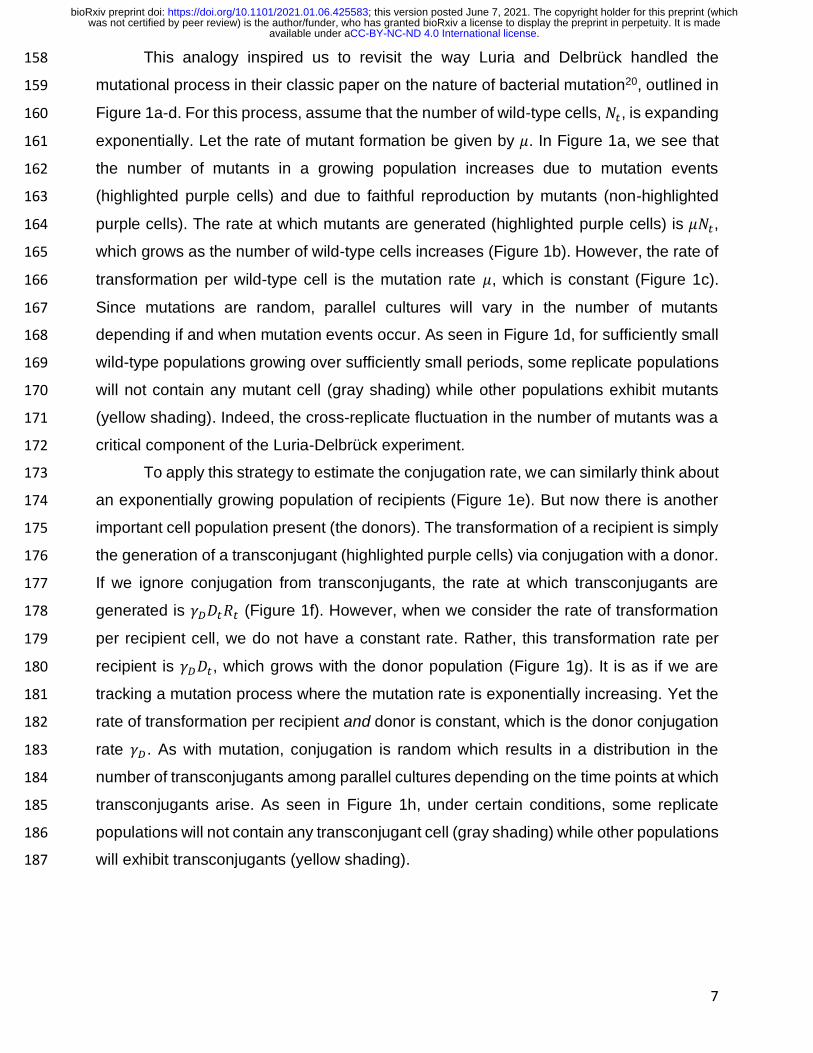
This analogy inspired us to revisit the way Luria and Delbrück handled the 158
mutational process in their classic paper on the nature of bacterial mutation20, outlined in 159
Figure 1a-d. For this process, assume that the number of wild-type cells, 𝑁𝑡, is expanding 160
exponentially. Let the rate of mutant formation be given by 𝜇. In Figure 1a, we see that 161
the number of mutants in a growing population increases due to mutation events 162
(highlighted purple cells) and due to faithful reproduction by mutants (non-highlighted 163
purple cells). The rate at which mutants are generated (highlighted purple cells) is 𝜇𝑁𝑡, 164
which grows as the number of wild-type cells increases (Figure 1b). However, the rate of 165
transformation per wild-type cell is the mutation rate 𝜇, which is constant (Figure 1c). 166
Since mutations are random, parallel cultures will vary in the number of mutants 167
depending if and when mutation events occur. As seen in Figure 1d, for sufficiently small 168
wild-type populations growing over sufficiently small periods, some replicate populations 169
will not contain any mutant cell (gray shading) while other populations exhibit mutants 170
(yellow shading). Indeed, the cross-replicate fluctuation in the number of mutants was a 171
critical component of the Luria-Delbrück experiment. 172
To apply this strategy to estimate the conjugation rate, we can similarly think about 173
an exponentially growing population of recipients (Figure 1e). But now there is another 174
important cell population present (the donors). The transformation of a recipient is simply 175
the generation of a transconjugant (highlighted purple cells) via conjugation with a donor. 176
If we ignore conjugation from transconjugants, the rate at which transconjugants are 177
generated is 𝛾𝐷𝐷𝑡𝑅𝑡 (Figure 1f). However, when we consider the rate of transformation 178
per recipient cell, we do not have a constant rate. Rather, this transformation rate per 179
recipient is 𝛾𝐷𝐷𝑡, which grows with the donor population (Figure 1g). It is as if we are 180
tracking a mutation process where the mutation rate is exponentially increasing. Yet the 181
rate of transformation per recipient and donor is constant, which is the donor conjugation 182
rate 𝛾𝐷. As with mutation, conjugation is random which results in a distribution in the 183
number of transconjugants among parallel cultures depending on the time points at which 184
transconjugants arise. As seen in Figure 1h, under certain conditions, some replicate 185
populations will not contain any transconjugant cell (gray shading) while other populations 186
will exhibit transconjugants (yellow shading). 187
.CC-BY-NC-ND 4.0 International licenseavailable under awas not certified by peer review) is the author/funder, who has granted bioRxiv a license to display the preprint in perpetuity. It is made
The copyright holder for this preprint (whichthis version posted June 7, 2021. ; https://doi.org/10.1101/2021.01.06.425583doi: bioRxiv preprint

8
Figure 1: Schematic comparing the process of mutation (a-d) to the process of conjugation (e-h). (a) In a growing population of wild-type cells, mutants arise (highlighted purple cells) and reproduce (non-highlighted purple cells). (b) The rate at which mutants are generated grows as the number of wild-type cells increases at rate 𝜇𝑁𝑡. (c) The rate of transformation per wild-type cell is the mutation rate 𝜇. (d) Wild-type cells growing in 9 separate populations where mutants arise in a proportion of the populations (yellow background) at different cell divisions. Here, for each tree, time progresses from top to bottom (rather than left to right as in part a). (e) In a growing population of donors and recipients, transconjugants arise (highlighted purple cells) and reproduce (non-highlighted purple cells). (f) The rate at which transconjugants are generated grows as the numbers of donors and recipients increase at rate 𝛾𝐷𝐷𝑡𝑅𝑡. (g) The rate of transformation per recipient cell grows as the number of donors increases at a rate 𝛾𝐷𝐷𝑡, where 𝛾𝐷 is the constant conjugation rate. (h) Donor and recipient cells growing in 9 separate populations where transconjugants arise in a proportion of the populations (yellow background) at different points in time (which again, here, progresses top to bottom for each tree).
.CC-BY-NC-ND 4.0 International licenseavailable under awas not certified by peer review) is the author/funder, who has granted bioRxiv a license to display the preprint in perpetuity. It is made
The copyright holder for this preprint (whichthis version posted June 7, 2021. ; https://doi.org/10.1101/2021.01.06.425583doi: bioRxiv preprint

9
Using this analogy, here we describe a new approach for estimating conjugation 188
rate which embraces conjugation as a stochastic process21. Let the density of donors, 189
recipients and transconjugants in a well-mixed culture at time 𝑡 be given by the variables 190
𝐷𝑡, 𝑅𝑡, and 𝑇𝑡. In all that follows, we will assume that the culture is inoculated with donors 191
and recipients, while transconjugants are initially absent (i.e., 𝐷0 > 0, 𝑅0 > 0, and 𝑇0 =192
0). The donor and recipient populations grow according to the following standard 193
exponential growth equations 194
𝐷𝑡 = 𝐷0𝑒𝜓𝐷𝑡 , [7]
𝑅𝑡 = 𝑅0𝑒𝜓𝑅𝑡 , [8]
where 𝜓𝐷 and 𝜓𝑅 are the growth rates for donor and recipient cells, respectively. With 195
equations [7] and [8], we are making a few assumptions, which also occur in some of the 196
previous methods (see SI Table 3 for a comparison). First, we assume that donors and 197
recipients grow exponentially. Given that we focus on low-density culture conditions 198
where nutrients are plentiful, this assumption will be reasonable. Second, we assume that 199
population growth for these two strains is deterministic (i.e., 𝐷𝑡 and 𝑅𝑡 are not random 200
variables). As long as the numbers of donors and recipients are not too small (i.e., 𝐷0 ≫201
0 and 𝑅0 ≫ 0), this assumption is acceptable. Lastly, we assume the loss of recipient cells 202
to transformation into transconjugants can be ignored. For what follows, the rate of 203
generation of transconjugants per recipient cell (as in Figure 1g) is very small relative to 204
the per capita recipient growth rate, making this last assumption justifiable. 205
The population growth of transconjugants is modeled using a continuous-time 206
stochastic process. The number of transconjugants, 𝑇𝑡, is a random variable taking on 207
non-negative integer values. In this section, we will assume the culture volume is 1 ml 208
and thus the number of transconjugants (i.e., cfu) is equivalent to the density of 209
transconjugants (i.e., cfu per ml). For a very small interval of time, Δ𝑡, the current number 210
of transconjugants will either increase by one or remain constant. The probabilities of 211
each possibility are given as follows: 212
Pr{𝑇𝑡+Δ𝑡 = 𝑇𝑡 + 1} = 𝛾𝐷𝐷𝑡𝑅𝑡Δ𝑡 + 𝛾𝑇𝑇𝑡𝑅𝑡Δ𝑡 + 𝜓𝑇𝑇𝑡Δ𝑡, [9]
Pr{𝑇𝑡+Δ𝑡 = 𝑇𝑡} = 1 − (𝛾𝐷𝐷𝑡𝑅𝑡 + 𝛾𝑇𝑇𝑡𝑅𝑡 + 𝜓𝑇𝑇𝑡)Δ𝑡. [10]
The three terms on the right-hand side of equation [9] illustrate the processes enabling 213
the transconjugant population to increase. The first term gives the probability that a donor 214
.CC-BY-NC-ND 4.0 International licenseavailable under awas not certified by peer review) is the author/funder, who has granted bioRxiv a license to display the preprint in perpetuity. It is made
The copyright holder for this preprint (whichthis version posted June 7, 2021. ; https://doi.org/10.1101/2021.01.06.425583doi: bioRxiv preprint
10
transforms a recipient into a transconjugant via conjugation (𝛾𝐷). The second term gives 215
the probability that a transconjugant transforms a recipient via conjugation (𝛾𝑇). The third 216
term measures the probability that a transconjugant cell divides (𝜓𝑇 is the transconjugant 217
growth rate). Equation [10] is simply the probability that none of these three processes 218
occur. 219
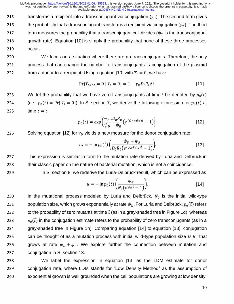
We focus on a situation where there are no transconjugants. Therefore, the only 220
process that can change the number of transconjugants is conjugation of the plasmid 221
from a donor to a recipient. Using equation [10] with 𝑇𝑡 = 0, we have 222
Pr{𝑇𝑡+Δ𝑡 = 0 | 𝑇𝑡 = 0} = 1 − 𝛾𝐷𝐷𝑡𝑅𝑡Δ𝑡. [11]
We let the probability that we have zero transconjugants at time 𝑡 be denoted by 𝑝0(𝑡) 223
(i.e., 𝑝0(𝑡) = Pr{ 𝑇𝑡 = 0}). In SI section 7, we derive the following expression for 𝑝0(𝑡) at 224
time 𝑡 = �̃�: 225
𝑝0(�̃�) = exp {−𝛾𝐷𝐷0𝑅0𝜓𝐷 + 𝜓𝑅
(𝑒(𝜓𝐷+𝜓𝑅)𝑡 − 1)}. [12]
Solving equation [12] for 𝛾𝐷 yields a new measure for the donor conjugation rate: 226
𝛾𝐷 = − ln𝑝0(�̃�) (𝜓𝐷 + 𝜓𝑅
𝐷0𝑅0(𝑒(𝜓𝐷+𝜓𝑅)𝑡 − 1)
). [13]
This expression is similar in form to the mutation rate derived by Luria and Delbrück in 227
their classic paper on the nature of bacterial mutation, which is not a coincidence. 228
In SI section 8, we rederive the Luria-Delbrück result, which can be expressed as 229
𝜇 = − ln𝑝0(�̃�) (𝜓𝑁
𝑁0(𝑒𝜓𝑁𝑡 − 1)). [14]
In the mutational process modeled by Luria and Delbrück, 𝑁0 is the initial wild-type 230
population size, which grows exponentially at rate 𝜓𝑁 . For Luria and Delbrück, 𝑝0(�̃�) refers 231
to the probability of zero mutants at time �̃� (as in a gray-shaded tree in Figure 1d), whereas 232
𝑝0(�̃�) in the conjugation estimate refers to the probability of zero transconjugants (as in a 233
gray-shaded tree in Figure 1h). Comparing equation [14] to equation [13], conjugation 234
can be thought of as a mutation process with initial wild-type population size 𝐷0𝑅0 that 235
grows at rate 𝜓𝐷 + 𝜓𝑅. We explore further the connection between mutation and 236
conjugation in SI section 13. 237
We label the expression in equation [13] as the LDM estimate for donor 238
conjugation rate, where LDM stands for “Low Density Method” as the assumption of 239
exponential growth is well grounded when the cell populations are growing at low density. 240
.CC-BY-NC-ND 4.0 International licenseavailable under awas not certified by peer review) is the author/funder, who has granted bioRxiv a license to display the preprint in perpetuity. It is made
The copyright holder for this preprint (whichthis version posted June 7, 2021. ; https://doi.org/10.1101/2021.01.06.425583doi: bioRxiv preprint

11
Indeed, this is how we conduct the assay to compute this estimate. The acronym can 241
alternatively stand for “Luria-Delbrück Method” given the connection to their approach. 242
243
Simulation Methods 244
To explore the accuracy and precision of the LDM estimate (as well as other 245
estimates), we developed a stochastic simulation framework using the Gillespie 246
algorithm. We extended the base model (equations [1] - [3]) to include plasmid loss due 247
to segregation at rate 𝜏. Specifically, transconjugants are transformed into plasmid-free 248
recipients due to plasmid loss via segregation at rate 𝜏𝑇. Similarly, the donors become 249
plasmid-free cells through segregative loss of the plasmid at rate 𝜏𝐷; therefore, the 250
extended model tracks the change in density of a new population type, plasmid-free 251
former donors (𝐹). In total, the extended model describes the density changes in four 252
populations (𝐷, 𝑅, 𝑇, and 𝐹) influenced by the values of various biological parameters: 253
growth rates (𝜓𝐷, 𝜓𝑅, 𝜓𝑇, and 𝜓𝐹), conjugation rates (𝛾𝐷 and 𝛾𝑇) and segregation rates 254
(𝜏𝐷 and 𝜏𝑇). For each simulation, we specify starting cell densities (𝐷0 > 0 and 𝑅0 > 0, 255
but always 𝑇0 = 𝐹0 = 0) and allow the four populations to grow and transform 256
stochastically for a specified incubation time �̃� in a 1 ml culture volume. The simulations 257
occur in sets, where each set involves a sweep across values of some key parameter. 258
Each sweep varies a biological process (i.e., growth, conjugation, or segregation) in 259
isolation to determine the effect on accuracy and precision of the donor conjugation rate 260
estimates. For instance, the transconjugant conjugation rate (𝛾𝑇) could be varied while all 261
other parameters are held constant. For each parameter setting within a sweep, ten 262
thousand parallel populations were simulated, and then conjugation rate was calculated 263
to yield replicate estimates for each method of interest (TDR, SIM, ASM, and LDM). 264
Notably, the LDM requires an estimate of the probability that a population has no 265
transconjugants at the end of the assay, which we denote �̂�0(�̃�). The maximum likelihood 266
estimate of this probability is the fraction of populations (i.e., parallel simulations) that 267
have no transconjugants at the specified incubation time �̃� (see SI section 9 for details). 268
Thus, for LDM, we calculated �̂�0(�̃�) at the specified incubation time �̃� by reserving multiple 269
parallel populations for each conjugation rate estimate. For more details on the 270
simulations such as the extended model equations, selection of the specified incubation 271
time �̃�, and calculation of each estimate see SI section 11. 272
273
274
.CC-BY-NC-ND 4.0 International licenseavailable under awas not certified by peer review) is the author/funder, who has granted bioRxiv a license to display the preprint in perpetuity. It is made
The copyright holder for this preprint (whichthis version posted June 7, 2021. ; https://doi.org/10.1101/2021.01.06.425583doi: bioRxiv preprint

12
Simulation Results 275
Exploring accuracy and sensitivity of the LDM and other conjugation methods 276
The underlying assumptions used to derive the various estimates for conjugation 277
rate (i.e., TDR, SIM, ASM, and LDM) entail simplifications of biological systems. To 278
explore the effects of violating these assumptions on the LDM and other conjugation rate 279
estimates, we used a stochastic simulation framework to investigate their accuracy across 280
a range of theoretical conditions. All of our simulated populations increase in size over 281
the incubation time, so a fundamental assumption of the TDR approach (i.e., no change 282
in the density due to growth) is broken for all of the runs. Here we divide our simulations 283
into three scenarios that break additional assumptions of at least one conjugation model 284
considered to this point: unequal growth rates, unequal conjugation rates, and a non-zero 285
segregation rate. When growth rates are different between populations, a modeling 286
assumption is violated for the TDR and SIM estimates. When donor and transconjugant 287
conjugation rates are unequal, a modeling assumption can be violated for the TDR, SIM, 288
and ASM estimates. When the segregation rate is non-zero, a modeling assumption is 289
violated for all of the estimates considered. We note that some of our parameter values 290
fall outside of reported values; these choices were made either to improve computational 291
speed or to better illustrate the effects of differences (e.g., in growth or transfer rates). 292
However, many of the parameter values used to explore the effects of incubation time 293
were set to reported parameter values. 294
295
The effect of unequal growth rates 296
Plasmid-containing hosts often incur a cost or gain a benefit in terms of growth rate 297
for plasmid carriage relative to plasmid-free hosts. We simulated a range of growth-rate 298
effects on plasmid-containing hosts from large plasmid costs (𝜓𝐷 = 𝜓𝑇 ≪ 𝜓𝑅) to large 299
plasmid benefits (𝜓𝐷 = 𝜓𝑇 ≫ 𝜓𝑅). The LDM estimate had high accuracy and precision 300
across all parameter settings (Figure 2a). The ASM estimate performed similarly to the 301
LDM estimate with regards to the mean value for each parameter setting (Figure 2a, black 302
horizontal lines). Given that the ASM was developed to allow for unequal growth rates, 303
its mean accuracy conforms to expectations. However, it is also worth noting that the 304
distribution of the ASM estimate was skewed for some of the parameter settings. In other 305
words, the mean (Figure 2a, black horizontal lines) is separated from the median (Figure 306
2a, green horizontal line); therefore, the average of a small number of replicates could 307
have led to a deviant mean estimate. The TDR and SIM estimates were inaccurate for 308
.CC-BY-NC-ND 4.0 International licenseavailable under awas not certified by peer review) is the author/funder, who has granted bioRxiv a license to display the preprint in perpetuity. It is made
The copyright holder for this preprint (whichthis version posted June 7, 2021. ; https://doi.org/10.1101/2021.01.06.425583doi: bioRxiv preprint
13
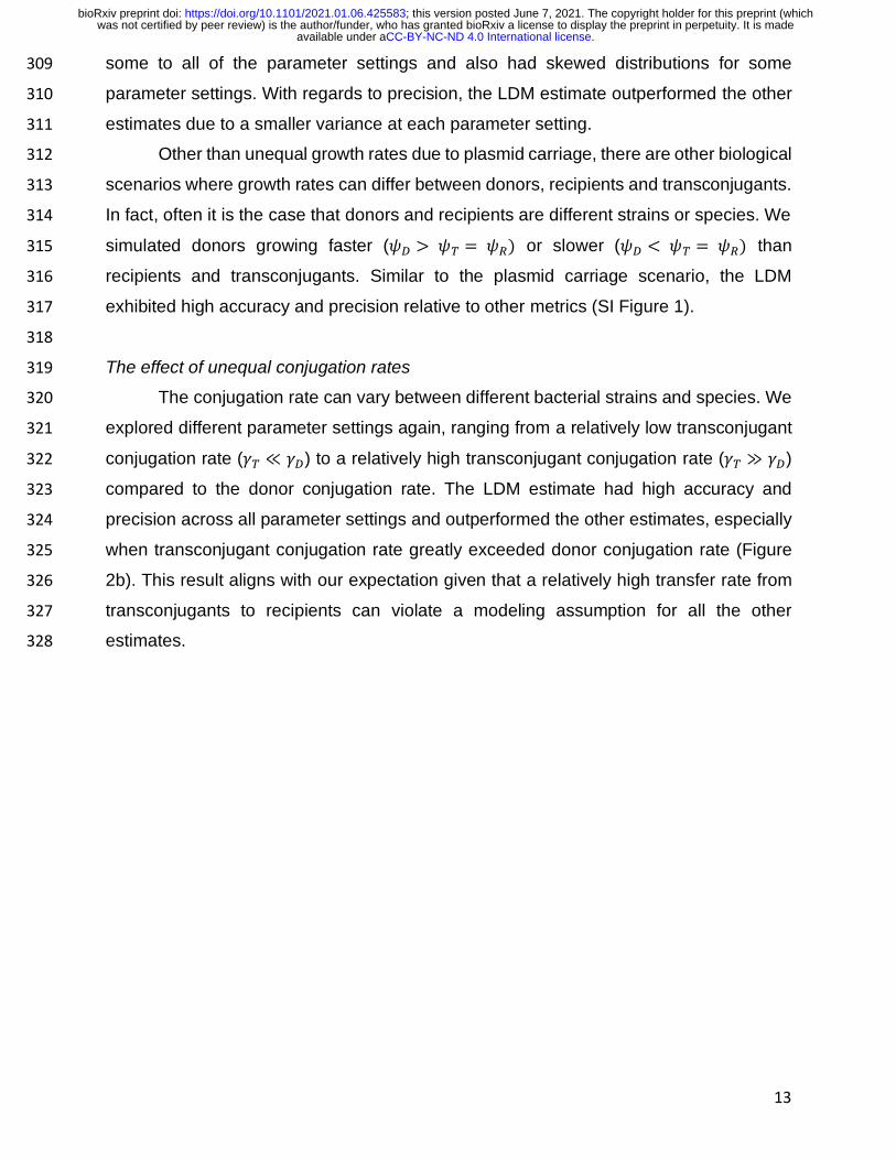
some to all of the parameter settings and also had skewed distributions for some 309
parameter settings. With regards to precision, the LDM estimate outperformed the other 310
estimates due to a smaller variance at each parameter setting. 311
Other than unequal growth rates due to plasmid carriage, there are other biological 312
scenarios where growth rates can differ between donors, recipients and transconjugants. 313
In fact, often it is the case that donors and recipients are different strains or species. We 314
simulated donors growing faster (𝜓𝐷 > 𝜓𝑇 = 𝜓𝑅) or slower (𝜓𝐷 < 𝜓𝑇 = 𝜓𝑅) than 315
recipients and transconjugants. Similar to the plasmid carriage scenario, the LDM 316
exhibited high accuracy and precision relative to other metrics (SI Figure 1). 317
318
The effect of unequal conjugation rates 319
The conjugation rate can vary between different bacterial strains and species. We 320
explored different parameter settings again, ranging from a relatively low transconjugant 321
conjugation rate (𝛾𝑇 ≪ 𝛾𝐷) to a relatively high transconjugant conjugation rate (𝛾𝑇 ≫ 𝛾𝐷) 322
compared to the donor conjugation rate. The LDM estimate had high accuracy and 323
precision across all parameter settings and outperformed the other estimates, especially 324
when transconjugant conjugation rate greatly exceeded donor conjugation rate (Figure 325
2b). This result aligns with our expectation given that a relatively high transfer rate from 326
transconjugants to recipients can violate a modeling assumption for all the other 327
estimates. 328
.CC-BY-NC-ND 4.0 International licenseavailable under awas not certified by peer review) is the author/funder, who has granted bioRxiv a license to display the preprint in perpetuity. It is made
The copyright holder for this preprint (whichthis version posted June 7, 2021. ; https://doi.org/10.1101/2021.01.06.425583doi: bioRxiv preprint

14
Figure 2 : The effect of violating various modeling assumptions on estimating conjugation rate. The Gillespie algorithm was used to simulate population dynamics. The parameter values were 𝜓𝐷 = 𝜓𝑅 = 𝜓𝑇 = 1, 𝛾𝐷 = 𝛾𝑇 =1 × 10⁻⁶, and 𝜏𝐷 = 𝜏𝑇 = 0 unless otherwise indicated. The dynamic variables were initialized with 𝐷0 = 𝑅0 = 1 × 10² and 𝑇0 = 𝐹0 = 0. All incubation times are short but are specific to each parameter setting (see SI section 11 for details).
Conjugation rate was estimated using 10,000 populations and summarized using boxplots. The gray dashed line indicates the “true” value for the donor conjugation rate. The box contains the 25th to 75th percentile. The vertical lines connected to the box contain 1.5 times the interquartile range above the 75th percentile and below the 25th percentile with the caveat that the whiskers were always constrained to the range of the data. The colored line in the box indicates the median. The solid black line indicates the mean. The boxplots in gray indicate the baseline parameter setting, and all colored plots represent deviation of one or two parameters from baseline. (a) Unequal growth rates were explored over a range of growth rates for the plasmid-bearing strains, namely 𝜓𝐷 = 𝜓𝑇 ∈ {0.0625, 0.125, 0.25, 0.5, 1, 2, 4, 8}. (b) Unequal conjugation rates were probed over a range of transconjugant conjugation rates, namely 𝛾𝑇 ∈{10−9, 10−8, 10−7, 10−6, 10−5, 10−4, 10−3, 10−2}. (c) We also explored the process of segregation by considering a range of segregative loss rates 𝜏𝐷 = 𝜏𝑇 ∈ {0, 0.0001, 0.001, 0.001, 0.01}.
.CC-BY-NC-ND 4.0 International licenseavailable under awas not certified by peer review) is the author/funder, who has granted bioRxiv a license to display the preprint in perpetuity. It is made
The copyright holder for this preprint (whichthis version posted June 7, 2021. ; https://doi.org/10.1101/2021.01.06.425583doi: bioRxiv preprint

15
The effect of a non-zero segregation rate 329
Plasmid loss due to segregation is a common occurrence in plasmid populations 330
and violates a model assumption underlying all the conjugation rate estimates. We 331
simulated a range of segregative loss rates, ranging from low (𝜏𝐷 = 𝜏𝑇 = 0.0001) to high 332
(𝜏𝐷 = 𝜏𝑇 = 0.1). The LDM had high accuracy and precision across all parameter settings 333
(Figure 2c). The effect of segregation was undetectable even for an extremely high 334
segregation rate (𝜏𝐷 = 𝜏𝑇 = 0.1). Similarly, the effect of segregative loss was undetectable 335
on the other conjugation estimates compared to their performance without any 336
segregative loss (Figure 2c, colored vs. grey box plots). Thus, we find that all estimates 337
appear robust with regards to an introduction of the process of segregation. 338
339
Case studies to explore the effects of incubation time 340
The incubation time �̃� is an important consideration for executing all conjugation 341
rate assays in the laboratory. Often the incubation time is variable for estimates of 342
conjugation rate reported in the literature. We explored the effects of altering incubation 343
time by estimating conjugation rate at 30-minute intervals. Since these estimates rely on 344
measuring different quantities, the range for the 30-minute sampling intervals differ 345
between estimates. For the TDR, SIM, and ASM estimates, the range for these intervals 346
was determined by the condition that at least 90 percent of the simulated populations 347
contained transconjugants at the incubation time �̃�. Specifically, we note that equations 348
[4], [5], and [6] all require 𝑇𝑡 > 0 for a non-zero conjugation rate estimate. This contrasts 349
with the LDM since this estimate needs some parallel populations to be absent of 350
transconjugants. Specifically, equation [13] requires 0 < 𝑝0(�̃�) < 1 for a non-zero finite 351
conjugation rate estimate. Thus, for the LDM estimate, the range for the sampling 352
intervals was determined by the condition that at least one parallel population had zero 353
transconjugants. Therefore, estimates for the LDM are shown at earlier incubation times 354
than those for the other methods (Figure 3). 355
.CC-BY-NC-ND 4.0 International licenseavailable under awas not certified by peer review) is the author/funder, who has granted bioRxiv a license to display the preprint in perpetuity. It is made
The copyright holder for this preprint (whichthis version posted June 7, 2021. ; https://doi.org/10.1101/2021.01.06.425583doi: bioRxiv preprint

16
Figure 3 : The effect of incubation time (�̃�) on estimating conjugation rate. The Gillespie algorithm was used to
simulate population dynamics with 𝜓𝐷 = 𝜓𝑅 = 𝜓𝑇 = 1, 𝛾𝐷 = 𝛾𝑇 = 1 × 10⁻¹⁴, and 𝜏𝐷 = 𝜏𝑇 = 0 unless otherwise
indicated. The dynamic variables were initialized with 𝐷0 = 𝑅0 = 1 × 10⁵ and 𝑇0 = 𝐹0 = 0. Conjugation rate was
estimated for 100 populations and summarized using boxplots. The gray dashed line indicates the “true” value for the donor conjugation rate. Each box contains the 25th to 75th percentile. The vertical lines connected to the box contain 1.5 times the interquartile range above the 75th percentile and below the 25th percentile with the caveat that the whiskers were always constrained to the range of the data. The colored line in the box indicates the median. The solid black line indicates the mean. (a) An unequal growth rate was simulated with 𝜓𝐷 = 𝜓𝑇 = 0.07. (b) An unequal conjugation rate
was simulated with 𝛾𝑇 = 1 × 10⁻⁹. (c) We simulated a positive segregation rate with 𝜏𝐷 = 𝜏𝑇 = 0.01.
.CC-BY-NC-ND 4.0 International licenseavailable under awas not certified by peer review) is the author/funder, who has granted bioRxiv a license to display the preprint in perpetuity. It is made
The copyright holder for this preprint (whichthis version posted June 7, 2021. ; https://doi.org/10.1101/2021.01.06.425583doi: bioRxiv preprint

17
We ran simulations with parameter values for growth and conjugation rates which 356
are reported in the literature (𝜓𝐷 = 𝜓𝑅 = 𝜓𝑇 = 𝜓𝐹 = 1, 𝛾𝐷 = 𝛾𝑇 = 1 × 10⁻¹⁴) and 357
reasonable initial densities (𝐷0 = 𝑅0 = 1 × 10⁵). As before, each biological scenario 358
examined a perturbation to a single biological parameter (i.e., growth, conjugation, or 359
segregation) to determine the effect on accuracy and precision. For the scenario exploring 360
growth differences, we added a plasmid cost (Figure 3a, 𝜓𝐷 = 𝜓𝑇 = 0.7). For the scenario 361
highlighting unequal conjugation rates, we increased the conjugation rate of 362
transconjugants (Figure 3b, 𝛾𝑇 = 1 × 10⁻⁹). For the scenario incorporating segregation, 363
we simply chose a rather high segregation rate (Figure 3c, 𝜏𝐷 = 𝜏𝑇 = 0.01). 364
The LDM estimate had high accuracy over all time points for all scenarios with 365
precision increasing through time. The other estimates also became more precise over 366
time. However, their greater precision over time was sometimes accompanied by 367
increasing inaccuracy (Figure 3b). Again, the LDM estimate performed as well or better 368
than other estimates across incubation times. 369
370
The LDM Implementation 371
In this section we describe the general experimental procedure for estimating 372
donor conjugation rate (𝛾𝐷) using the LDM estimate in the laboratory. The assay can 373
accommodate a wide variety of microbial species and conjugative plasmids since our 374
estimate allows for distinct growth and conjugation rates. In SI section 6, we rearrange 375
equation [13] to this alternative form for implementing the LDM in the laboratory: 376
𝛾𝐷 = 𝑓 {1
�̃�[− ln �̂�0(�̃�)]
ln𝐷𝑡𝑅𝑡 − ln𝐷0𝑅0𝐷𝑡𝑅𝑡 − 𝐷0𝑅0
}. [15]
Similar to previous conjugation estimates, the LDM requires measurement of initial and 377
final densities of donors and recipients (𝐷0, 𝑅0, 𝐷𝑡, and 𝑅𝑡). In addition, the LDM requires 378
an estimate of the probability that a population has no transconjugants at the end of the 379
assay, which we denote �̂�0(�̃�). The maximum likelihood estimate of this probability is the 380
fraction of populations (i.e., parallel mating cultures) that have no transconjugants at the 381
specified incubation time �̃� (see SI section 9 for details). Cell densities are generally 382
measured in cfu
ml units and the conjugation rate in
ml
h ∙ cfu units, thus, the standard unit of 383
volume in these assays is a milliliter. If exactly 1 ml is used as the volume for each mating 384
culture (as assumed in previous sections), then the quantity in braces in equation [15] is 385
the estimate for the conjugation rate. However, smaller mating volumes can be 386
advantageous (e.g., 100 l in a well inside a microtiter plate). When the mating volume 387
.CC-BY-NC-ND 4.0 International licenseavailable under awas not certified by peer review) is the author/funder, who has granted bioRxiv a license to display the preprint in perpetuity. It is made
The copyright holder for this preprint (whichthis version posted June 7, 2021. ; https://doi.org/10.1101/2021.01.06.425583doi: bioRxiv preprint

18
deviates from 1 ml, we must add a correction factor 𝑓 which is the number of experimental 388
volume units (evu) per ml (e.g., for a mating volume of 100 l, we would have 𝑓 = 10evu
ml, 389
see SI section 10 for details). 390
For a given incubation time (�̃�) and initial densities of donors (𝐷0) and recipients 391
(𝑅0), there will be some probability that transconjugants form (1 − 𝑝0(�̃�)). The 392
combinations of times and densities where this probability is not close to zero or one is 393
hereafter referred to as “the conjugation window”. That is, for these time-density 394
combinations, there is a good chance that some mating cultures will result in 395
transconjugants, while others do not. For fixed initial donor and recipient densities, the 396
conjugation window refers to the time period where transconjugants are first expected to 397
form. Determining the conjugation window provides the researcher with target initial 398
densities of donors (𝐷0′ ) and recipients (𝑅0
′ ) and target incubation times (�̃�′). Note we add 399
primes to the target time-density combination to set them apart from 𝐷0, 𝑅0, and �̃� in 400
equation [15] which will be gathered in the conjugation assay itself. 401
To determine the conjugation window and find a time-density combination, we mix 402
exponentially growing populations of donors and recipients in a large array of parallel 403
mating cultures for a full factorial treatment of initial densities and incubation times (Figure 404
4a and 4b). For ease of presentation, we will assume that donors and recipients start at 405
equal proportion and we will refer to the “initial density” as the total cell density of these 406
two strains. In our schematic, columns of a 96 deep well microtiter plate are grouped by 407
the value of the initial density (3 columns per value; Figure 4a) and rows are grouped by 408
the value of the incubation time (2 rows per value; Figure 4b). At each time in the set of 409
incubation times being explored, growth medium selecting for transconjugants (see SI 410
section 12 for explanation) is added. This dilutes the mating cultures by ten-fold, which 411
hinders further conjugation and simultaneously permits the growth of any transconjugant 412
cells that previously formed (Figure 4b). After a longer incubation, we assess the mating 413
cultures (3 columns x 2 rows = 6 wells; Figure 4c) within each time-density treatment for 414
presence or absence of transconjugants (i.e., turbid culture or non-turbid culture). There 415
are three possible outcomes for each treatment: all matings have transconjugants, none 416
of the matings have transconjugants, or there is both transconjugant-containing and 417
transconjugant-free matings. We are interested in the last outcome (Figure 4c, gray dots). 418
These treatments meet the �̂�0(�̃�) condition (i.e., 0 < �̂�0(�̃�) < 1) thus identifying a valid 419
time-density combination for the LDM conjugation assay. As a general expectation, 420
mating cultures with high donor conjugation rates (𝛾𝐷) will require shorter incubation times 421
.CC-BY-NC-ND 4.0 International licenseavailable under awas not certified by peer review) is the author/funder, who has granted bioRxiv a license to display the preprint in perpetuity. It is made
The copyright holder for this preprint (whichthis version posted June 7, 2021. ; https://doi.org/10.1101/2021.01.06.425583doi: bioRxiv preprint

19
than mating cultures with low donor conjugation rates for a given initial density. We note 422
that there will generally be multiple time-density treatments in the conjugation window 423
and the final treatment choice may be determined by experimental tractability. Thus, this 424
choice is not constrained and can be made based on an incubation time that is practically 425
feasible. In addition, the LDM does not require the initial density of donors and recipients 426
to be identical (as was assumed for this presentation). Indeed, in certain circumstances 427
it may be easier to have donor and recipient initial densities be unequal. 428
The chosen treatment yields the target time-density combination (𝐷0′ , 𝑅0
′ , �̃�′), and 429
we proceed with executing the LDM conjugation assay to gather all components to 430
estimate the conjugation rate. We mix exponentially growing populations of donors and 431
recipients, inoculate many mating cultures at the target initial density (𝐷0′+𝑅0
′ ) in a 96 deep 432
well plate, and incubate in non-selective growth medium for the target incubation time (�̃�′) 433
(Figure 4d). We note that the incubation time �̃� may deviate slightly from the target 434
incubation time �̃�′ due to timing constraints in the laboratory, but small deviations are 435
generally permissible. Thus, the executed incubation time �̃� should be used to calculate 436
the conjugation rate. To estimate the initial densities (𝐷0 and 𝑅0), three mating cultures at 437
the start of the assay are diluted and plated on donor-selecting and recipient-selecting 438
agar plates. We note that the initial densities (𝐷0 and 𝑅0) may deviate from the target 439
initial densities (𝐷0′ and 𝑅0
′ ), but small deviations are permissible. After the incubation time 440
�̃�, final densities (𝐷𝑡 and 𝑅𝑡) are obtained by dilution-plating from the same mating 441
cultures. Growth medium selecting for transconjugants is subsequently added to the 442
remaining mating cultures. To obtain �̂�0(�̃�), we assess the proportion of mating cultures 443
that are non-turbid after incubation in transconjugant-selecting medium, as these cultures 444
have no transconjugants (Figure 4d). This differs from the traditional Luria–Delbrück 445
method since no plating is required to obtain �̂�0(�̃�). The binary output (turbidity vs. no 446
turbidity) is assessed in a high throughput manner using a standard microtiter 447
spectrophotometer. Using the obtained densities (𝐷0, 𝑅0, 𝐷𝑡, and 𝑅𝑡), the incubation time 448
(�̃�), the proportion of transconjugant-free populations (�̂�0(�̃�)), and correcting for the 449
experimental culture volume (𝑓), the LDM estimate for donor conjugation rate (𝛾𝐷) can be 450
calculated via equation [15]. 451
.CC-BY-NC-ND 4.0 International licenseavailable under awas not certified by peer review) is the author/funder, who has granted bioRxiv a license to display the preprint in perpetuity. It is made
The copyright holder for this preprint (whichthis version posted June 7, 2021. ; https://doi.org/10.1101/2021.01.06.425583doi: bioRxiv preprint

20
Figure 4 : Overview for finding the conjugation window (a-c) and executing the LDM conjugation assay (d). (a) Microtiter plate map designating placement of donors (red), recipients (blue), transconjugants (purple), and mating cultures over 10-fold dilutions (different shades of gray). For simplicity, donors and recipients are at the same proportion in each mating culture. The control wells are the last three columns. (b) Using the microtiter plate from part a, transconjugant-selecting medium (green well fill) is added at each time period designated by two rows in the microtiter plate. Two example wells from different time-density treatments are highlighted on the left where the gray background shading refers to the initial density treatment labeled in part a. In the top example well, transconjugant-selecting medium is added immediately, inhibiting growth of donor and recipient cells (grey dashed cells), and resulting in a non-turbid well as no transconjugants formed. In the bottom example well, the donor and recipient populations in the mating culture grow until transconjugant-selecting medium is added at 9-hours, inhibiting growth of donors and recipients, and permitting growth of the formed transconjugants. (c) After a lengthy incubation of the microtiter plate from part b, there are two well-types in the microtiter plate (bottom-left): transconjugant-containing (green well with purple cross) and transconjugant-free (green well). For each treatment (time-density pair), the 6 mating wells are considered as a group, resulting in one of three outcomes (top): all transconjugant-free wells (white dot), all transconjugant-containing wells (black dot), a proportion of both well-types (gray dot). Any treatment with a gray dot represents a viable combination of initial densities (𝐷0
′ + 𝑅0′ ) and incubation time (�̃�′). (d) The microtiter plate is set up with many matings (gray) at the
chosen target density (𝐷0′ +𝑅0
′ ) in addition to control wells. Three matings are sampled to determine the actual initial
.CC-BY-NC-ND 4.0 International licenseavailable under awas not certified by peer review) is the author/funder, who has granted bioRxiv a license to display the preprint in perpetuity. It is made
The copyright holder for this preprint (whichthis version posted June 7, 2021. ; https://doi.org/10.1101/2021.01.06.425583doi: bioRxiv preprint

21
densities (𝐷0 and 𝑅0) and final densities (𝐷�̃� and 𝑅�̃�). After the incubation time (�̃�), which is as close to the target incubation time (�̃�′) as possible, transconjugant-selecting medium is added to the microtiter plate (excluding the matings used for density-plating). After a lengthy incubation, the proportion of transconjugant-free (i.e., non-turbid) wells is calculated, yielding �̂�0(�̃�). Using the actual incubation time (�̃�), initial densities (𝐷0, 𝑅0), final densities (𝐷�̃�, 𝑅�̃�), and correcting for the experimental culture volume (𝑓), the LDM estimate is used to calculate donor conjugation rate (𝛾𝐷). Part d can be repeated to obtain replicate LDM estimates.
Application of the LDM 452
To explore the logistics of implementing the LDM, we measured the conjugation 453
rate of a conjugative, IncP-1 plasmid (pALTS29) encoding chloramphenicol resistance 454
in an Escherichia coli host4. Jordt et. al.4 used this plasmid-host pair as an ancestral strain 455
which was propagated in chloramphenicol antibiotic for 400 generations to explore 456
mechanisms of plasmid-host co-evolution. The evolved lineage acquired genetic 457
modifications in the host chromosome and the plasmid. The ancestral plasmid was 458
gradually lost from the ancestral host population when these plasmid-bearing cells were 459
propagated under conditions that did not select for the plasmid (Figure 5a, dashed line). 460
In contrast, the evolved plasmid was considerably more persistent in the absence of 461
selection in its co-evolved host (Figure 5a, solid line). 462
This pattern of increased plasmid persistence after plasmid-host co-evolution is 463
consistent with previous studies22,23. In most cases, the cost of plasmid carriage is 464
assumed to decrease with plasmid-host co-evolution; however, changes in other factors, 465
such as an increased rate of conjugation or a decreased rate of segregational loss, may 466
also result in increased plasmid persistence. Using the LDM method, we showed that the 467
observed increase in plasmid persistence in the Jordt. et. al.4 study is at least in part due 468
to a significant increase in the conjugation rate in the evolved lineage (Figure 5b, Mann-469
Whitney U test, p-value = 0.029). 470
Figure 5 : LDM conjugation rate estimates of an ancestral and evolved lineage of E. coli containing a
conjugative IncP-1 plasmid. (a) Plasmid persistence in the absence of chloramphenicol antibiotic was higher in the evolved plasmid-host pair (solid line) than the ancestral plasmid-host pair (dashed line). Data and figure adapted from Jordt et. al.4 (b) Conjugation rate significantly increased in the evolved (Evo) plasmid-host pair compared to the ancestral (Anc) plasmid-host pair. The points represent a conjugation rate estimate from an LDM conjugation assay. The black line is the mean of four replicates. The colored line is the median of the four replicates. The asterisk indicates a significant difference from a Mann-Whitney U test.
.CC-BY-NC-ND 4.0 International licenseavailable under awas not certified by peer review) is the author/funder, who has granted bioRxiv a license to display the preprint in perpetuity. It is made
The copyright holder for this preprint (whichthis version posted June 7, 2021. ; https://doi.org/10.1101/2021.01.06.425583doi: bioRxiv preprint

22
Discussion 471
Here we have presented a new method for estimating the rate of plasmid 472
conjugative transfer from a donor cell to a recipient cell. We derived our LDM estimate 473
using a mathematical approach that captures the stochastic process of conjugation, which 474
was inspired by the method Luria and Delbrück applied to the process of mutation. This 475
departs from the mathematical approach for other conjugation rate estimates which 476
assume underlying deterministic frameworks guiding the dynamics of 477
transconjugants11,13,16. One noteworthy conjugation assay from Johnson & Kroer also 478
embraced the stochastic nature of conjugation21. Similar to one aspect of our approach, 479
they survey a series of mating cultures for the presence of transconjugants and use the 480
fraction of transconjugant-free cultures to derive a conjugation metric. However, their 481
metric yields the number of conjugation events and does not provide an estimate for the 482
conjugation rate. Thus, the population dynamics of donors and recipients, as well as the 483
incubation time, are not considered. The LDM captures positive features of both the 484
Johnson & Kroer approach and the deterministic-based approaches: specifically, it both 485
recognizes the stochastic nature of conjugation and provides an analytic estimate for the 486
conjugation rate. 487
Beyond the incorporation of stochasticity, the model and derivation behind the 488
LDM estimate relaxes assumptions that constrained former approaches. This makes 489
calculating conjugation rates accessible to a wide range of experimenters that use 490
different plasmid-donor-recipient combinations. The LDM estimate makes no restrictive 491
assumptions about growth rates or conjugation rates of different bacterial strains. Other 492
conjugation rate estimates assume little to no change in the density due to growth (TDR), 493
growth rates are identical across all strains (TDR and SIM), conjugation rates are identical 494
for donors and transconjugants (SIM), or conjugation events from transconjugants are 495
few (TDR and ASM)11,13,16. By relaxing these assumptions, we have increased the 496
applicability of this new estimate, and our simulation results confirmed the high accuracy 497
of the LDM under such scenarios. In contrast, the other conjugation methods (TDR, SIM, 498
and ASM) sometimes yielded inaccurate estimates when their underlying assumptions 499
were violated. Because violations of these assumptions are likely in natural plasmid 500
systems, these performance differences could be important. For instance, unequal growth 501
rates can occur among isogenic strains if the plasmid increases or decreases the growth 502
rate of a host5,24. Also, growth rates may be significantly different when the donor and 503
recipient are different strains or species. For example, some strains of Escherichia coli 504
.CC-BY-NC-ND 4.0 International licenseavailable under awas not certified by peer review) is the author/funder, who has granted bioRxiv a license to display the preprint in perpetuity. It is made
The copyright holder for this preprint (whichthis version posted June 7, 2021. ; https://doi.org/10.1101/2021.01.06.425583doi: bioRxiv preprint

23
can divide every 20 minutes while some strains of Shewanella oneidensis only divide 505
every 45 minutes25,26. Consequently, the growth rates of all the cell types will differ due 506
to these combined effects in many plasmid transfer experiments. Such compounding 507
effects could increase the error in measuring conjugation rate with the TDR and SIM 508
estimates. Moreover, unequal growth rates are not likely to occur in isolation, but in 509
tandem with other modeling violations such as unequal plasmid transfer rates. The 510
consequences of such scenarios remain to be explored. 511
Perhaps the most significant advantage of our LDM method is the capability to 512
accurately estimate the donor conjugation rate when it deviates from the transconjugant 513
conjugation rate. For the previous methods, the error in estimating the donor conjugation 514
rate increases as the transconjugant conjugation rate gets larger than the donor 515
conjugation rate. These differences are likely to occur in plasmid transfer experiments. 516
For instance, Dimitriu et. al.27 used the TDR approach to measure donor conjugation rate 517
where the recipient was a clone-mate or a different species. The authors observed cross-518
species conjugation rates that were up to 4 orders of magnitude lower than the within-519
species conjugation rates. If this pattern held generally, then a cross-species mating 520
assay would violate a key assumption of previous methods, in that the transconjugant 521
conjugation rate would be much higher than the donor conjugation rate. Indeed, the 522
“unequal conjugation rates” simulations resulted in inflated conjugation estimates for the 523
other methods (Figure 2b). For these reasons, reported cross-species conjugation rates 524
may also be overestimates. In any case, unequal conjugation rates are likely, especially 525
in microbial communities with diverse species. In addition, unequal conjugation rates can 526
arise due to a molecular mechanism encoded on the conjugative plasmid, such as 527
transitory de-repression13,28. In this case, a conjugation event between donor and 528
recipient will temporarily elevate the conjugation rate of the newly formed transconjugant. 529
This phenomenon would lead to similar outcomes as described above for different 530
species. The LDM method can accurately estimate donor conjugation rates in systems 531
with unequal conjugation rates, whether the differences are taxonomic or molecular in 532
origin. 533
The LDM estimate also has advantages in terms of precision. Since conjugation is 534
a stochastic process, the number of transconjugants at any given time is a random 535
variable with a certain distribution. Therefore, estimates that rely on the number of 536
transconjugants (TDR, SIM and ASM) or the probability of their absence (LDM) will also 537
fall into distributions (Figure 2). Even in cases where the mean (first moment of the 538
.CC-BY-NC-ND 4.0 International licenseavailable under awas not certified by peer review) is the author/funder, who has granted bioRxiv a license to display the preprint in perpetuity. It is made
The copyright holder for this preprint (whichthis version posted June 7, 2021. ; https://doi.org/10.1101/2021.01.06.425583doi: bioRxiv preprint

24
distribution) is close to the actual conjugation rate, the variance (second central moment) 539
may differ among estimates. In fact, the LDM estimate had smaller variance compared to 540
other estimates, even under parameter settings where different estimates shared similar 541
accuracy (Figure 2). This greater precision likely originates from the difference in the 542
distribution of the number of transconjugants (𝑇�̃�) and the distribution of the probability of 543
transconjugant absence (𝑝0(�̃�)), something we explore analytically in SI section 14. 544
Beyond the mean and variance, other features of these distributions (i.e., moments) may 545
also be important. For certain parameter settings, the estimates relying on transconjugant 546
numbers were asymmetric (the third moment was non-zero). In such cases, a small 547
number of replicate estimates could lead to bias. For example, when there is a strong 548
growth benefit to carrying the plasmid, the distribution for the ASM estimate is skewed 549
even though the mean of this distribution reflects the actual conjugation rate (see Figure 550
2a). Typically a small number of conjugation assays is often the standard in studies; thus, 551
the general position and shape of these estimate distributions may matter. Over the 552
portion of parameter space we explored, the LDM distribution facilitated accurate and 553
precise estimates through its position (a mean reflecting the true value) and its shape (a 554
small variance and a low skew). 555
For all the methods considered, the distribution of conjugation estimates changed 556
with time (Figure 3). Therefore, the incubation time becomes an important parameter. In 557
our simulations, the estimate distribution generally narrowed with longer incubation times 558
(Figure 3). This would suggest that one advantage of longer incubation is greater 559
precision. However, when underlying assumptions are violated, there can be an 560
interesting interaction between accuracy and precision over time. For instance, consider 561
the case where transconjugant conjugation rate exceeds donor conjugation rate (Figure 562
3b). For the SIM and ASM metrics, as incubation time rises, there is a shift from an 563
accurate imprecise estimate to an inaccurate precise estimate. For an assay with a limited 564
number of replicates in such a case, the optimal incubation time may be intermediate (a 565
topic worthy of formal investigation). Over a range of incubation times where 𝑝0(�̃�) is not 566
close to 0 or 1, the LDM distribution is generally immune to these problems, exhibiting 567
constant high accuracy and precision over time (Figure 3). 568
To execute a conjugation assay using any of the methods described, the 569
experimenter needs to make several decisions regarding various protocol features such 570
as incubation time and density of the mating culture. All of these choices need to conform 571
closely to the modeling assumptions of each method and ideally maximize the accuracy 572
.CC-BY-NC-ND 4.0 International licenseavailable under awas not certified by peer review) is the author/funder, who has granted bioRxiv a license to display the preprint in perpetuity. It is made
The copyright holder for this preprint (whichthis version posted June 7, 2021. ; https://doi.org/10.1101/2021.01.06.425583doi: bioRxiv preprint

25
of the conjugation rate estimate. For instance, the TDR assay seems simpler than the 573
other methods, since it only requires measurement of the final densities of cells. However, 574
implementing the TDR assay can be difficult because it assumes little to no change in 575
density due to growth. For a growth-based TDR implementation, a very short incubation 576
time could limit cell growth, but the density of the culture may need to be very high so 577
transconjugants can form during the assay. Previous studies have shown that for many 578
plasmids the conjugation rate is maximal during exponential phase13,17,29; therefore, using 579
high density culture may underestimate the conjugation rate. A chemostat implementation 580
could circumvent some of these issues by allowing lower density culture, exponential 581
growth, and longer incubation times. However, unequal growth rates in a chemostat 582
would lead to changes in the density of the donors and recipients. For the SIM approach, 583
a standard growth-based 24-hour conjugation assay is often used5,30,31,32,33. This serves 584
as an easy default choice and has many laboratory benefits for efficiency. Even so, the 585
24-hour incubation involves more than initial and final sampling, as two additional 586
samplings are required to measure the maximum population growth rate during 587
exponential phase (SI section 2). If these additional samplings are forgotten for the SIM 588
approach, highly inaccurate estimates of the conjugation rate can result. In addition, the 589
underlying SIM assumptions of equal growth rates and conjugation rates are easy to 590
violate, and inaccuracies due to such violations can grow with incubation time (Figure 3b). 591
For the ASM, a standard incubation time is not recommended; rather, this time is left to 592
the experimenter to determine. However, the authors suggest short incubation times to 593
prevent biased estimates if modeling assumptions are violated (e.g., relatively high 594
transconjugant transfer rates). The authors mention that a follow-up assay to measure 595
the transconjugant transfer rate may be needed to determine if the incubation time was 596
short enough to prevent deviations. In contrast, the LDM protocol is designed to lead the 597
experimenter to valid incubation times by explicitly identifying the conjugation window 598
where 𝑝0(�̃�) can be estimated. Therefore, the experimenter can be sure the protocol 599
occurred during a usable incubation time if the assay results in a �̂�0(�̃�) between 0 and 1. 600
We note that identifying the conjugation window does add an extra step in the LDM 601
approach; however, a similar assay could help an experimenter choose an optimal 602
incubation time for the other assays. Even so, the effects of these implementation choices 603
on the accuracy and precision of conjugation rate estimates are currently understudied. 604
The LDM protocol offers an additional advantage by eliminating plating of the 605
transconjugants. For the other methods, this is typically a source of error since the 606
.CC-BY-NC-ND 4.0 International licenseavailable under awas not certified by peer review) is the author/funder, who has granted bioRxiv a license to display the preprint in perpetuity. It is made
The copyright holder for this preprint (whichthis version posted June 7, 2021. ; https://doi.org/10.1101/2021.01.06.425583doi: bioRxiv preprint

26
transconjugant density is often determined by plating the mating culture on 607
transconjugant selecting medium. With short culture incubation times before plating, 608
which will increase the accuracy of the other methods, the transconjugant density is 609
extremely low compared to the donor and recipient densities. Therefore, plating high 610
density cultures is needed to be able to detect the transconjugants. This can lead to 611
conjugation continuing on the agar plates, which produces extra transconjugant colonies 612
that did not result from conjugation events before plating,15,34. Such ‘matings on 613
transconjugant-selecting agar plates’ can occur before the donors and recipients are 614
completely inhibited by the transconjugant-selecting agent (typically an antibiotic). Such 615
events will lead to an inflation of the transconjugant density and thus inaccuracy in the 616
conjugation rate estimate. We note that the LDM avoids this problem since it relies only 617
on recording transconjugant presence/absence in the liquid mating cultures. 618
We applied our high-throughput LDM protocol to our previous evolution experiment 619
to estimate the conjugation rate for an IncP-1 plasmid in an E. coli host. Interestingly, 620
we observed the evolution of conjugation rate. This comes as a bit of a surprise given 621
that the environment in which the E. coli evolved contained an antibiotic selecting for 622
plasmid carriage. Thus, plasmid-free cells would have been rare leading to few 623
opportunities for plasmid conjugation into such cells. Bacterial cells containing a 624
conjugative plasmid in a community with an abundance of plasmid-free cells is the 625
scenario in which conjugation rates are expected to and have been observed to evolve35. 626
Therefore, it is not immediately obvious what mechanism led to the increase in the 627
conjugation rate in our system. It is possible that increased conjugation rate could have 628
been a pleiotropic effect from a different trait under direct selection. Alternatively, higher 629
conjugation rate could evolve if (1) a mutation on the plasmid led to a higher transfer rate 630
and (2) if donor cells can conjugate with other donors in our systems36. In such a case, 631
the mutated plasmid would transfer quickly even under plasmid-selecting conditions and 632
it could spread through the population as long as any associated costs (e.g., lower growth 633
of its host or lower replication efficiency within mixed-plasmid hosts) were sufficiently low. 634
This hypothetical sequence of events could lead to an increased conjugation rate. 635
Regardless of the mechanism, it is interesting that bacterial populations in environments 636
containing an antibiotic could lead to the evolution of higher conjugation rates of plasmids 637
encoding resistance to that antibiotic. Importantly, such evolution could lead to higher 638
frequency of antibiotic resistance in microbial communities, even in the absence of the 639
antibiotic, due to more plasmid conjugation events. 640
.CC-BY-NC-ND 4.0 International licenseavailable under awas not certified by peer review) is the author/funder, who has granted bioRxiv a license to display the preprint in perpetuity. It is made
The copyright holder for this preprint (whichthis version posted June 7, 2021. ; https://doi.org/10.1101/2021.01.06.425583doi: bioRxiv preprint

27
In conclusion, the LDM offers new possibilities for measuring the conjugation rate 641
for many types of plasmids and species. We have presented evidence that supports our 642
method being more accurate and precise than other widely used approaches. We note 643
that we did not fully review all the conjugation assays currently in use in the literature15,37, 644
focusing instead on the least laborious and most widely used methods. Importantly, the 645
LDM eliminates the possible bias caused by high transconjugant conjugation rates. Due 646
to the sensitivity of the LDM conjugation assay and the ease of implementation, we were 647
able to show the evolution of conjugation rate for an IncP-1 conjugative plasmid in an 648
Escherichia coli host. However, the LDM method can be applied even more broadly given 649
the flexibility of the underlying theoretical framework and the relative ease of assay 650
implementation. 651
652
Acknowledgements 653
This work is supported by the National Institute of Allergy and Infectious Diseases 654
Extramural Activities grant no. R01 AI084918 of the National Institutes of Health. O.K. is 655
supported by the NSF Graduate Research Fellowship grant no. DGE-1762114. C.E. is 656
supported by the NSF Graduate Research Fellowship. We thank Hannah Jordt, Simon 657
Snoeck, and members of the Kerr and Top laboratories for useful suggestions on the 658
manuscript. 659
.CC-BY-NC-ND 4.0 International licenseavailable under awas not certified by peer review) is the author/funder, who has granted bioRxiv a license to display the preprint in perpetuity. It is made
The copyright holder for this preprint (whichthis version posted June 7, 2021. ; https://doi.org/10.1101/2021.01.06.425583doi: bioRxiv preprint

28
Supplemental Information660
SI section 1 : Historical theoretical perspective 661
In this section, we highlight three key methods for estimating conjugation rate. 662
While outlining the theoretical framework, we highlight the key distinctions and theoretical 663
assumptions of each approach. Levin et. al.13 introduced a simple mathematical model 664
for plasmid population dynamics to isolate the conjugation rate parameter (𝛾)13. In their 665
model, the donor population grows exponentially at a rate 𝜓 (equation [1]). The number 666
of transconjugants increases due to conjugation events (2nd term equation [3]) by donors 667
and by existing transconjugants as well as exponential growth of the existing 668
transconjugant pool (1st term equation [3]). The recipient population grows exponentially 669
at a rate 𝜓 and is depleted at the rate that new transconjugants form due to conjugation 670
events (2nd term equation [2]). For ease of reference, model variables and parameters 671
are in SI Table 1 (the LDM is included for a complete comparison). 672
SI Table 1: Variables and parameters used in plasmid dynamic models
Variable/Parameter Description Relevant Estimate Units
𝐷 Donor density TDR, SIM, ASM, LDM
cfu
ml 𝑅 Recipient density TDR, SIM, ASM, LDM
𝑇 Transconjugant density TDR, SIM, ASM, LDM
𝜓 Growth rate (not population specific) TDR, SIM
1
h
𝜓𝐷 Donor growth rate ASM, LDM
𝜓𝑅 Recipient growth rate ASM, LDM
𝜓𝑇 Transconjugant growth rate ASM, LDM
𝛾 Conjugation rate (not population specific) TDR, SIM
ml
cfu ∙ h 𝛾𝐷 Donor-recipient conjugation rate ASM, LDM
𝛾𝑇 Transconjugant-recipient conjugation rate ASM, LDM
Equations [1] - [3] contains four notable assumptions. First, conjugation is 673
described by mass-action kinetics, where conjugation events are proportional to the 674
product of donor and recipient cell densities, which is a reasonable assumption in well-675
mixed liquid cultures13. Second, the model assumes a negligible rate of segregation, a 676
process whereby a dividing plasmid-containing cell produces one plasmid-containing 677
daughter cell and one plasmid-free daughter. These first two assumptions also exist in all 678
.CC-BY-NC-ND 4.0 International licenseavailable under awas not certified by peer review) is the author/funder, who has granted bioRxiv a license to display the preprint in perpetuity. It is made
The copyright holder for this preprint (whichthis version posted June 7, 2021. ; https://doi.org/10.1101/2021.01.06.425583doi: bioRxiv preprint

29
of the other conjugation estimate methods we discuss. Third, the growth rate is the same 679
for all cell types (donors, recipients, and transconjugants). Fourth, the plasmid 680
conjugation rate is the same from donors to recipients as from transconjugants to 681
recipients. 682
Levin et. al.13 used their plasmid dynamic model to derive an estimate for plasmid 683
conjugation rate (𝛾) by making three additional simplifying assumptions. First, the change 684
in cell density of donors due to growth is assumed to be negligible. Likewise, the change 685
in cell density of recipients due to growth and to conjugation (i.e., transformation into 686
transconjugants) is assumed to be negligible. Finally, transconjugants are assumed to be 687
rare in the population resulting in negligible growth of transconjugants and conjugation 688
from transconjugants to recipients. Thus, the increase in transconjugants cell density is 689
through plasmid conjugation from donors to recipients (i.e., 𝑑𝑇/𝑑𝑡 = 𝛾𝐷𝑅). Using these 690
simplifying assumptions, Levin et. al.13 solved for an expression of the conjugation rate 𝛾 691
(equation [4]) in terms of the density of donors, recipients, and transconjugants (𝐷𝑡, 𝑅𝑡, 692
and 𝑇𝑡, respectively) after a period of incubation �̃� (see SI section 3 for a few different 693
approaches to this derivation). We label the expression in equation [4] as the “TDR” 694
estimate for the conjugation rate, where the letters in this acronym come from the dynamic 695
variables used in the estimate. TDR is a commonly used estimate14,13,15,17. However, the 696
simplifying assumptions used to derive TDR, such as no change in density due to growth, 697
can make implementation in the laboratory difficult. For ease of reference, all variables 698
used in the conjugation estimates are in SI Table 2. All assumptions underlying each 699
estimate are in SI Table 3. Both tables include LDM for a full comparison. 700
SI Table 2: Variables and parameters used to estimate* conjugation rate
Variable/Parameter Description Relevant Estimate Units
�̃� Incubation time (final sampling time) TDR, SIM**, ASM, LDM h
𝐷0, 𝑅0 Initial donor and recipient densities ASM, LDM
cfu
ml
𝐷𝑡 , 𝑅𝑡 Final donor and recipient densities TDR, SIM, ASM, LDM
𝑇𝑡 Final transconjugant density TDR, SIM, ASM
𝑁0, 𝑁𝑡 Initial and final total population density SIM
𝜓𝑇 Transconjugant growth rate ASM h−1
𝑝0(�̃�) Probability a population has no transconjugants
LDM exp (cfu
ml)
* The laboratory estimates are used here (see SI section 6) ** If the SIM assay is conducted on exponentially growing cultures (see SI section 2), 𝑡̃ along with 𝑁0 and 𝑁�̃� can be used to estimate 𝜓 (otherwise, an independent estimate of 𝜓 is needed).
.CC-BY-NC-ND 4.0 International licenseavailable under awas not certified by peer review) is the author/funder, who has granted bioRxiv a license to display the preprint in perpetuity. It is made
The copyright holder for this preprint (whichthis version posted June 7, 2021. ; https://doi.org/10.1101/2021.01.06.425583doi: bioRxiv preprint

30
SI Table 3: Summary of modeling assumptions
Assumption TDR SIM ASM LDM
Conjugation events follow mass-action kinetics X X X X
There is no segregative loss of the plasmid X X X X
The cell populations do not change in size due to growth X
Processes of conjugation and growth are not resource dependent* X X X
The cell populations grow exponentially X X
The growth rate is identical for all cell types X X
The transconjugant conjugation rate is not high relative to the donor conjugation rate
X X X
* The SIM model is able to incorporate resource-dependent growth and conjugation because (1) growth and transfer rates are homogeneous and (2) the functional form for resource dependence is the same for growth and transfer.
In contrast to the assumption behind the TDR estimate, the model explored by 701
Simonsen et. al.16 allows for population growth. Indeed, they allowed for the rate of 702
population growth to change with the level of a resource in the environment, adding a 703
dynamic variable for the resource concentration. In addition, the conjugation rate can also 704
change with the resource concentration. The authors focus on a case where both growth 705
and conjugation rates vary with resource concentration according to the Monod function. 706
This choice was informed by experimental results showing that cells enter stationary 707
phase and conjugation ramps down to a negligible level as resources are depleted13. This 708
pattern occurs for various plasmid incompatibility groups, but not all29. Simonsen et. al.16 709
used this updated model to derive an estimate for plasmid conjugation rate (equation [5], 710
see SI section 4 for the derivation). We term equation [5] as the “SIM” estimate for 711
conjugation rate, where SIM stands for “Simonsen et. al. Identicality Method” since the 712
underlying model assumes that all strains are identical with regards to growth, and donors 713
and transconjugants are identical with regards to conjugation rate (as in equations [1]-714
[3]). The SIM estimate involves measuring the density of the initial population (𝑁0), and 715
the final density of donors (𝐷𝑡), recipients (𝑅𝑡), transconjugants (𝑇𝑡), and the total 716
population (𝑁𝑡) after the incubation time �̃� (e.g., the end of an assay). The SIM estimate 717
is a commonly used since it allows for the use of batch culture in the laboratory. Thus, it 718
circumvents the constraints of the laboratory implementation of TDR; however, the 719
underlying model (an enriched version of equations [1]-[3]) holds the same assumptions 720
as before: homogeneous growth rates and conjugation rates. 721
.CC-BY-NC-ND 4.0 International licenseavailable under awas not certified by peer review) is the author/funder, who has granted bioRxiv a license to display the preprint in perpetuity. It is made
The copyright holder for this preprint (whichthis version posted June 7, 2021. ; https://doi.org/10.1101/2021.01.06.425583doi: bioRxiv preprint

31
Recently, Huisman et. al.11 updated the SIM model by introducing population 722
specific growth rates for donors, recipients, and transconjugants (𝜓𝐷, 𝜓𝑅, and 𝜓𝑇, 723
respectively) and population specific conjugation rates for donors and transconjugants 724
(𝛾𝐷 and 𝛾𝑇). Importantly, the updated model is an approximation of the SIM due to three 725
additional assumptions. First, conjugation and growth rates are assumed to be constant 726
until resources are depleted, eliminating the additional resource concentration equation. 727
Second, the increase in recipients due to growth greatly outpaces the decrease in 728
recipients due to conjugation (i.e., 𝜓𝑅𝑅 ≫ 𝛾𝐷𝐷𝑅 + 𝛾𝑇𝑇𝑅). Third, the increase in 729
transconjugants due to growth or plasmid conjugation from donors to recipients greatly 730
outpaces the increase in transconjugants due to plasmid conjugation from 731
transconjugants to recipients (i.e., 𝜓𝑇𝑇 + 𝛾𝐷𝐷𝑅 ≫ 𝛾𝑇𝑇𝑅). These model conditions are 732
reasonable if the system starts with donors and recipients present but transconjugants 733
are absent, the system is tracked for a short period of time �̃�, conjugation rates are low 734
relative to growth rates, and the transconjugant conjugation rate (𝛾𝑇) is not much higher 735
than the donor conjugation rate (𝛾𝐷). With these added assumptions, equations [1]-[3] 736
can be reformulated as the following approximate system of equations: 737
𝑑𝐷
𝑑𝑡= 𝜓𝐷𝐷, [1.1]
𝑑𝑅
𝑑𝑡= 𝜓𝑅𝑅, [1.2]
𝑑𝑇
𝑑𝑡= 𝜓𝑇𝑇 + 𝛾𝐷𝐷𝑅, [1.3]
Huisman et. al. use this model to derive an estimate for conjugation rate (equation [6]) 738
where different cell types now can have different growth rates (see SI section 5 for the 739
derivation). We term equation [6] as the ASM estimate for donor conjugation rate, where 740
ASM stands for “Approximate Simonsen et. al. Method”. 741
742
SI section 2 : Comparison of laboratory implementations 743
In this section, we compare the laboratory implementations for various end-point 744
estimates: TDR, SIM, and ASM. Each method is explained either as recommended by its 745
authors or the most simplified protocol to acquire the information for the estimate. For 746
each, we describe proper laboratory implementation for the approaches based on the 747
model and derivation assumptions used to acquire the estimate. Note in this section, we 748
do not explore the assumptions that are violated due to the biological samples being 749
.CC-BY-NC-ND 4.0 International licenseavailable under awas not certified by peer review) is the author/funder, who has granted bioRxiv a license to display the preprint in perpetuity. It is made
The copyright holder for this preprint (whichthis version posted June 7, 2021. ; https://doi.org/10.1101/2021.01.06.425583doi: bioRxiv preprint
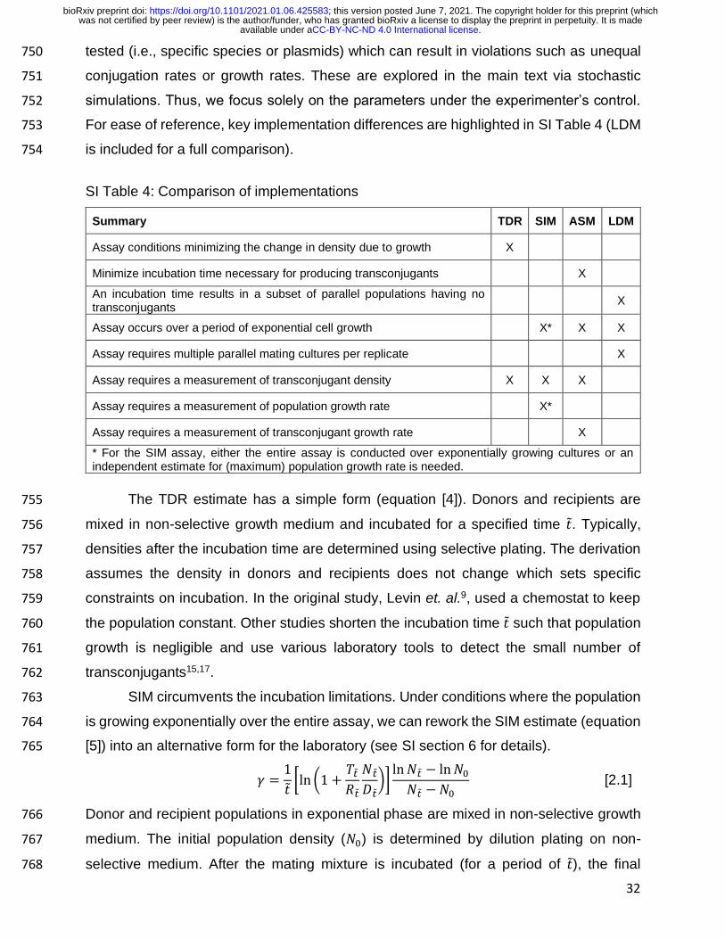
32
tested (i.e., specific species or plasmids) which can result in violations such as unequal 750
conjugation rates or growth rates. These are explored in the main text via stochastic 751
simulations. Thus, we focus solely on the parameters under the experimenter’s control. 752
For ease of reference, key implementation differences are highlighted in SI Table 4 (LDM 753
is included for a full comparison). 754
SI Table 4: Comparison of implementations
Summary TDR SIM ASM LDM
Assay conditions minimizing the change in density due to growth X
Minimize incubation time necessary for producing transconjugants X
An incubation time results in a subset of parallel populations having no transconjugants
X
Assay occurs over a period of exponential cell growth X* X X
Assay requires multiple parallel mating cultures per replicate X
Assay requires a measurement of transconjugant density X X X
Assay requires a measurement of population growth rate X*
Assay requires a measurement of transconjugant growth rate X
* For the SIM assay, either the entire assay is conducted over exponentially growing cultures or an independent estimate for (maximum) population growth rate is needed.
The TDR estimate has a simple form (equation [4]). Donors and recipients are 755
mixed in non-selective growth medium and incubated for a specified time �̃�. Typically, 756
densities after the incubation time are determined using selective plating. The derivation 757
assumes the density in donors and recipients does not change which sets specific 758
constraints on incubation. In the original study, Levin et. al.9, used a chemostat to keep 759
the population constant. Other studies shorten the incubation time �̃� such that population 760
growth is negligible and use various laboratory tools to detect the small number of 761
transconjugants15,17. 762
SIM circumvents the incubation limitations. Under conditions where the population 763
is growing exponentially over the entire assay, we can rework the SIM estimate (equation 764
[5]) into an alternative form for the laboratory (see SI section 6 for details). 765
𝛾 =1
�̃�[ln (1 +
𝑇𝑡𝑅𝑡
𝑁𝑡𝐷𝑡)]ln𝑁𝑡 − ln𝑁0𝑁𝑡 −𝑁0
[2.1]
Donor and recipient populations in exponential phase are mixed in non-selective growth 766
medium. The initial population density (𝑁0) is determined by dilution plating on non-767
selective medium. After the mating mixture is incubated (for a period of �̃�), the final 768
.CC-BY-NC-ND 4.0 International licenseavailable under awas not certified by peer review) is the author/funder, who has granted bioRxiv a license to display the preprint in perpetuity. It is made
The copyright holder for this preprint (whichthis version posted June 7, 2021. ; https://doi.org/10.1101/2021.01.06.425583doi: bioRxiv preprint

33
densities (𝐷𝑡, 𝑅𝑡, 𝑇𝑡, and 𝑁𝑡) are determined by dilution plating on selective and non-769
selective media. To implement SIM as written in equation [2.1], the specified incubation 770
time �̃� must occur well before stationary phase is reached to collect proper data for 771
estimating the population growth rate (𝜓 = (ln𝑁𝑡 − ln𝑁0)/�̃�). There is an alternative 772
option for implementing the SIM using equation [5]. The donor and recipient populations 773
are mixed and incubated under batch culture conditions (including lag, exponential, and 774
stationary phase). However, the (maximum) population growth rate (𝜓) needs to be 775
determined with two additional samplings from the mixed population at times 𝑡𝑎 and 𝑡𝑏, 776
both occurring within exponential phase: 777
𝜓 =ln (𝑁𝑡𝑏/𝑁𝑡𝑎)
𝑡𝑏 − 𝑡𝑎 [2.2]
The population densities 𝑁𝑡𝑎 and 𝑁𝑡𝑏 can be estimated either through colony counts from 778
plating or optical density from a spectrophotometer. Either way, the timing of exponential 779
phase is important for this approach and at least some analysis during this phase is 780
required regardless of the implementation strategy. 781
For the ASM estimate, we can rework equation [6] into an alternate form for the 782
laboratory (see SI section 6 for details). 783
𝛾𝐷 = {1
�̃�(ln𝐷𝑡𝑅𝑡 − ln𝐷0𝑅0) − 𝜓𝑇}
𝑇�̃�
(𝐷𝑡𝑅�̃� − 𝐷0𝑅0𝑒𝜓𝑇𝑡) [2.3]
Donor and recipient populations in exponential phase are mixed in non-selective medium. 784
Initial densities (𝐷0 and 𝑅0) are determined by plating dilutions on the appropriate 785
selective media. After donor and recipient incubate (�̃�), final densities (𝐷𝑡, 𝑅𝑡, and 𝑇�̃�) are 786
determined by plating dilutions on the appropriate selective media. From the 787
transconjugant-selecting agar plates, a transconjugant clone is incubated in monoculture 788
then sampled twice (at times 𝑡𝑎 and 𝑡𝑏) in exponential phase to measure the 789
transconjugant growth rate (𝜓𝑇 = ln(𝑇𝑡𝑏/𝑇𝑡𝑎)/(𝑡𝑏 − 𝑡𝑎)). The authors point out a critical 790
consideration for proper implementation of the ASM is the incubation time �̃�. Not only is 791
sampling in exponential phase important, but if the incubation time �̃� is too long and 792
passes a critical time (𝑡𝑐𝑟𝑖𝑡) the approximations used to derive the ASM break down. To 793
avoid overshooting 𝑡𝑐𝑟𝑖𝑡, the authors recommend sampling as soon as measurable 794
transconjugants arise. To determine that the incubation time used was below the critical 795
time (𝑡𝑐𝑟𝑖𝑡), a second assay is recommended by the authors to measure the 796
transconjugant conjugation rate 𝛾𝑇, which will determine if the original incubation time �̃� 797
was below 𝑡𝑐𝑟𝑖𝑡 for measuring the donor conjugation rate. This second assay would have 798
.CC-BY-NC-ND 4.0 International licenseavailable under awas not certified by peer review) is the author/funder, who has granted bioRxiv a license to display the preprint in perpetuity. It is made
The copyright holder for this preprint (whichthis version posted June 7, 2021. ; https://doi.org/10.1101/2021.01.06.425583doi: bioRxiv preprint

34
the transconjugant clone become the donor in the mixture, while a newly marked recipient 799
must be used so that donors and recipients can be distinguished using selective plating. 800
Each method has aspects of implementation in common. Each one shares the 801
basic approach of mixing donors and recipients over some incubation time �̃�. Each 802
estimate requires reliable selectable markers to differentiate donors, recipients, and 803
transconjugants. However, all estimates have some constraints on initial densities and 804
time of measurement. This can occur because the experimenter needs to capture 805
conjugation events (all estimates require this), avoid population growth (TDR), or keep 806
growth exponential (ASM, and at least parts of SIM). Even so, each method has clear 807
distinctions. The most notable is the incubation time �̃� (i.e., the end of the assay). The 808
TDR method is constrained to conditions where no change in population size due to 809
growth can occur. For SIM, initial and final sampling are not constrained to a particular 810
phase of growth; however, measurement of the growth rate must occur during the 811
exponential growth phase. For ASM, initial sampling is in early exponential phase, and 812
the final sampling needs to occur during a specific time window. In other words, the assay 813
needs to be long enough that measurable transconjugants appear, but short enough so 814
that assumptions aren’t violated (which can occur if transconjugant density becomes too 815
large). 816
817
SI section 3 : TDR derivation 818
We present a few derivations for the TDR method. The derivations differ by the 819
assumptions used to solve for TDR. We use this section to show all of the conditions 820
where the TDR method can be used. In addition, we use this section to walk through all 821
of the mathematical steps and provide an easy reference for comparing the derivations 822
of all four methods (TDR, SIM, ASM, and LDM). The original condition presented by Levin 823
et. al.13 is the last derivation described in this section. 824
Here we assume that we are considering conditions where population growth is 825
not occurring. These conditions could involve an environment hindering cell division. 826
Alternatively, the environment could promote growth, but we restrict the time period 827
sufficiently so that population change is negligible. Or finally, if all strains possess the 828
same growth rate, the population could be growing over longer periods of time but doing 829
so in a continuous flow-through device (e.g., a chemostat) such that population density 830
remains constant (see Levin et. al.13). Because we assume no segregative loss of the 831
plasmid, the donor population must remain constant 832
.CC-BY-NC-ND 4.0 International licenseavailable under awas not certified by peer review) is the author/funder, who has granted bioRxiv a license to display the preprint in perpetuity. It is made
The copyright holder for this preprint (whichthis version posted June 7, 2021. ; https://doi.org/10.1101/2021.01.06.425583doi: bioRxiv preprint

35
𝐷𝑡 = 𝐷0, [3.1]
for any time 𝑡 under consideration. Importantly, even though growth is not occurring, 833
conjugation can proceed. We assume 𝑇0 = 0, but the population of transconjugants can 834
increase over time. Because every transconjugant was formerly a recipient cell, it must 835
be the case that 836
𝑅𝑡 + 𝑇𝑡 = 𝑅0, 837
for any time 𝑡 under consideration. Therefore, 838
𝑅𝑡 = 𝑅0 − 𝑇𝑡. [3.2]
The dynamics of transconjugants is given by 839
𝑑𝑇𝑡𝑑𝑡
= 𝛾𝐷𝐷𝑡𝑅𝑡 + 𝛾𝑇𝑇𝑡𝑅𝑡 [3.3]
By substituting terms from equations [3.1] and [3.2] 840
𝑑𝑇𝑡𝑑𝑡
= 𝛾𝐷𝐷0(𝑅0 − 𝑇𝑡) + 𝛾𝑇𝑇𝑡(𝑅0 − 𝑇𝑡), 841
𝑑𝑇𝑡𝑑𝑡
= (𝛾𝐷𝐷0 + 𝛾𝑇𝑇𝑡)(𝑅0 − 𝑇𝑡), 842
𝑑𝑇𝑡𝑑𝑡
= −𝛾𝑇 (𝑇𝑡 +𝛾𝐷𝐷0𝛾𝑇
) (𝑇𝑡 − 𝑅0), 843
We can solve this differential equation by a separation of variables: 844
∫𝑑𝑇𝑡
−𝛾𝑇 (𝑇𝑡 +𝛾𝐷𝐷0𝛾𝑇
) (𝑇𝑡 − 𝑅0)
𝑡
0
= ∫ 𝑑𝑡𝑡
0
. 845
The following identity is relevant here: 846
𝑑 {1
𝑎(𝑏 − 𝑐)ln𝑥 − 𝑏𝑥 − 𝑐}
𝑑𝑥=
1
𝑎(𝑥 − 𝑏)(𝑥 − 𝑐) . 847
Letting 𝑥 = 𝑇𝑡, 𝑎 = −𝛾𝑇, 𝑏 = −𝛾𝐷𝐷0
𝛾𝑇, and 𝑐 = 𝑅0, we can proceed as follows: 848
{1
𝛾𝑇 (𝛾𝐷𝐷0𝛾𝑇
+ 𝑅0)ln𝑇𝑡 +
𝛾𝐷𝐷0𝛾𝑇
𝑇𝑡 − 𝑅0}|
0
𝑡
= (𝑡)|0𝑡 , 849
1
𝛾𝑇 (𝛾𝐷𝐷0𝛾𝑇
+ 𝑅0)(ln
𝑇𝑡 +𝛾𝐷𝐷0𝛾𝑇
𝑇�̃� − 𝑅0− ln
𝑇0 +𝛾𝐷𝐷0𝛾𝑇
𝑇0 − 𝑅0) = �̃�. 850
Because 𝑇0 = 0, 851
.CC-BY-NC-ND 4.0 International licenseavailable under awas not certified by peer review) is the author/funder, who has granted bioRxiv a license to display the preprint in perpetuity. It is made
The copyright holder for this preprint (whichthis version posted June 7, 2021. ; https://doi.org/10.1101/2021.01.06.425583doi: bioRxiv preprint

36
1
𝛾𝑇 (𝛾𝐷𝐷0𝛾𝑇
+ 𝑅0)(ln
𝑇𝑡 +𝛾𝐷𝐷0𝛾𝑇
𝑇𝑡 − 𝑅0− ln
𝛾𝐷𝐷0𝛾𝑇−𝑅0
) = �̃�, 852
1
𝛾𝑇 (𝛾𝐷𝐷0𝛾𝑇
+ 𝑅0)(ln
−𝑅0 (𝑇�̃� +𝛾𝐷𝐷0𝛾𝑇
)
𝛾𝐷𝐷0𝛾𝑇
(𝑇𝑡 − 𝑅0)) = �̃�, 853
ln1 +
𝛾𝑇𝑇𝑡𝛾𝐷𝐷0
1 −𝑇𝑡𝑅0
= (𝛾𝐷𝐷0 + 𝛾𝑇𝑅0)�̃�, [3.4]
1 +𝛾𝑇𝑇𝑡𝛾𝐷𝐷0
1 −𝑇𝑡𝑅0
= exp{(𝛾𝐷𝐷0 + 𝛾𝑇𝑅0)�̃�}, 854
1 +𝛾𝑇𝑇𝑡𝛾𝐷𝐷0
= (1 −𝑇𝑡𝑅0) exp{(𝛾𝐷𝐷0 + 𝛾𝑇𝑅0)�̃�}, 855
𝛾𝑇𝑇𝑡𝛾𝐷𝐷0
+𝑇𝑡𝑅0exp{(𝛾𝐷𝐷0 + 𝛾𝑇𝑅0)�̃�} = exp{(𝛾𝐷𝐷0 + 𝛾𝑇𝑅0)�̃�} − 1, 856
𝑇𝑡 [𝛾𝑇𝛾𝐷𝐷0
+1
𝑅0exp{(𝛾𝐷𝐷0 + 𝛾𝑇𝑅0)�̃�}] = exp{(𝛾𝐷𝐷0 + 𝛾𝑇𝑅0)�̃�} − 1, 857
𝑇𝑡 =𝑅0(exp{(𝛾𝐷𝐷0 + 𝛾𝑇𝑅0)�̃�} − 1)
𝛾𝑇𝑅0𝛾𝐷𝐷0
+ exp{(𝛾𝐷𝐷0 + 𝛾𝑇𝑅0)�̃�}. [3.5]
Thus, equation [3.5] is a general solution for the number of transconjugants at any time. 858
If we assume that 𝛾𝑇 = 0, then we can rewrite [3.4] as 859
ln1
1 −𝑇𝑡𝑅0
= 𝛾𝐷𝐷0�̃�, 860
− ln (1 −𝑇𝑡𝑅0) = 𝛾𝐷𝐷0�̃�, 861
𝛾𝐷 =− ln (1 −
𝑇𝑡𝑅0)
𝐷0�̃�. [3.6]
When 𝑅0 ≫ 𝑇�̃�, a first-order Taylor approximation ensures − ln (1 −𝑇�̃�
𝑅0) ≈
𝑇�̃�
𝑅0, and 862
therefore 863
𝛾𝐷 ≈
𝑇�̃�𝑅0𝐷0�̃�
, 864
𝛾𝐷 ≈𝑇�̃�
𝐷0𝑅0�̃� . 865
.CC-BY-NC-ND 4.0 International licenseavailable under awas not certified by peer review) is the author/funder, who has granted bioRxiv a license to display the preprint in perpetuity. It is made
The copyright holder for this preprint (whichthis version posted June 7, 2021. ; https://doi.org/10.1101/2021.01.06.425583doi: bioRxiv preprint

37
Because 𝐷𝑡 = 𝐷0 (see [3.1]) and 𝑅𝑡 ≈ 𝑅0 (when 𝑅0 ≫ 𝑇�̃� by [3.2]), we have 866
𝛾𝐷 ≈𝑇�̃�
𝐷𝑡𝑅𝑡 �̃� . 867
On the other hand, if we assume 𝛾𝐷 = 𝛾𝑇 = 𝛾, then we can rewrite [3.4] as 868
ln1 +
𝑇𝑡𝐷0
1 −𝑇𝑡𝑅0
= 𝛾(𝐷0 + 𝑅0)�̃�, 869
𝛾 =1
�̃�(𝐷0 + 𝑅0)ln1 +
𝑇𝑡𝐷0
1 −𝑇𝑡𝑅0
, 870
𝛾 =1
�̃�(𝐷0 + 𝑅0){ln (1 +
𝑇𝑡𝐷0) − ln (1 −
𝑇𝑡𝑅0)}. [3.7]
When 𝐷0 ≫ 𝑇𝑡 and 𝑅0 ≫ 𝑇𝑡, first-order Taylor approximations ensure 871
𝛾 ≈1
�̃�(𝐷0 + 𝑅0)(𝑇𝑡𝐷0+𝑇𝑡𝑅0), 872
𝛾 ≈𝑇�̃�
�̃�(𝐷0 + 𝑅0)(1
𝐷0+1
𝑅0), 873
𝛾 ≈𝑇�̃�
�̃�(𝐷0 + 𝑅0)(𝑅0+𝐷0𝐷0𝑅0
), 874
𝛾 ≈𝑇𝑡
𝐷0𝑅0�̃� . 875
Because 𝐷𝑡 = 𝐷0 and 𝑅𝑡 ≈ 𝑅0 (when 𝑅0 ≫ 𝑇𝑡), we have 876
𝛾 ≈𝑇𝑡
𝐷𝑡𝑅𝑡 �̃� . 877
So we have general expressions for donor conjugation rate when 𝛾𝑇 = 0 (equation [3.6]) 878
or when 𝛾𝐷 = 𝛾𝑇 (equation [3.7]). However, when 𝐷0 ≫ 𝑇𝑡 and 𝑅0 ≫ 𝑇𝑡, for all 𝑡 under 879
consideration, both of these measures are well approximated by equation [4]. Here we 880
extend the application of equation [4] even further. When 𝑅0 ≫ 𝑇𝑡, then 𝑅𝑡 ≈ 𝑅0. Let us 881
assume 𝑅𝑡 = 𝑅0. We will also assume 882
𝛾𝐷𝐷0𝑅0 ≫ 𝛾𝑇𝑇𝑡𝑅0, [3.8]
namely, the rate of formation of transconjugants by donors is much greater than the 883
formation by transconjugants. Of course, if 𝛾𝑇 = 0 or 𝛾𝐷 = 𝛾𝑇 , then 𝐷0 ≫ 𝑇𝑡 ensures 884
assumption [3.8]. However, assumption [3.8] does not require 𝛾𝑇 = 0 or 𝛾𝐷 = 𝛾𝑇 (indeed, 885
assumption [3.8] is satisfied when 𝛾𝐷 ≥ 𝛾𝑇 and 𝐷0 ≫ 𝑇𝑡, and 𝑅0 > 0). In general, this 886
inequality is satisfied when 𝑇0 = 0, 𝐷0 and 𝑅0 are is large, 𝛾𝑇 is not dramatically higher 887
.CC-BY-NC-ND 4.0 International licenseavailable under awas not certified by peer review) is the author/funder, who has granted bioRxiv a license to display the preprint in perpetuity. It is made
The copyright holder for this preprint (whichthis version posted June 7, 2021. ; https://doi.org/10.1101/2021.01.06.425583doi: bioRxiv preprint

38
than 𝛾𝐷, and the period is small. Under assumption [3.8], the dynamics can be well 888
approximated by a simplified version of the differential equation [3.3] (where the 889
transconjugant conjugation term is gone). This is the differential equation originally solved 890
by Levin et. al., 891
𝑑𝑇𝑡𝑑𝑡
= 𝛾𝐷𝐷0𝑅0. 892
Because everything on the right-hand-side of the equation is a constant, the solution is 893
straightforward: 894
∫ 𝑑𝑇𝑡
𝑡
0
= ∫ 𝛾𝐷𝐷0𝑅0𝑑𝑡𝑡
0
, 895
(𝑇𝑡)|0𝑡 = (𝛾𝐷𝐷0𝑅0𝑡)|0
𝑡 , 896
𝑇𝑡 − 𝑇0 = 𝛾𝐷𝐷0𝑅0�̃�. 897
Because 𝑇0 = 0, 898
𝑇𝑡 = 𝛾𝐷𝐷0𝑅0�̃�, 899
𝛾𝐷 =𝑇𝑡
𝐷0𝑅0�̃� . 900
Because 𝐷𝑡 = 𝐷0 and 𝑅𝑡 = 𝑅0 (by assumption), we have recovered equation [4]. 901
902
SI section 4 : SIM derivation 903
In this section, we walk through all of the mathematical steps in the Simonsen et. 904
al. derivation. We include this derivation as a quick reference to help the reader compare 905
the derivations of all four methods (TDR, SIM, ASM, and LDM). Simonsen et. al. modified 906
the model (equations [1]-[3]) by adding a dynamic variable for resource concentration (𝐶). 907
The dynamics of this resource incorporate an additional parameter for the amount of 908
resource needed to produce a new cell (𝑒). Both the growth rate and conjugation rate are 909
taken to be functions of the resource concentration. 910
𝑑𝐷
𝑑𝑡= 𝜓(𝐶)𝐷, [4.1]
𝑑𝑅
𝑑𝑡= 𝜓(𝐶)𝑅 − 𝛾(𝐶)𝑅(𝐷 + 𝑇), [4.2]
𝑑𝑇
𝑑𝑡= 𝜓(𝐶)𝑇 + 𝛾(𝐶)𝑅(𝐷 + 𝑇), [4.3]
𝑑𝐶
𝑑𝑡= −𝜓(𝐶)(𝑅 + 𝐷 + 𝑇)𝑒. [4.4]
.CC-BY-NC-ND 4.0 International licenseavailable under awas not certified by peer review) is the author/funder, who has granted bioRxiv a license to display the preprint in perpetuity. It is made
The copyright holder for this preprint (whichthis version posted June 7, 2021. ; https://doi.org/10.1101/2021.01.06.425583doi: bioRxiv preprint

39
The other variables are consistent with their use in equations [1]-[3]. In Simonsen et. al.16, 911
when resources are depleted, growth and conjugation stop. A Monod function introduces 912
batch culture dynamics (i.e., exponential and stationary phase) making growth and 913
conjugation both increase in a saturated manner with resource concentration, where the 914
resource concentration yielding ½ the maximal rate is given by the parameter 𝑄. 915
Importantly, conjugation and growth are assumed to have the same functional form: 916
𝜓(𝐶) =𝜓𝑚𝑎𝑥𝐶
𝑄 + 𝐶, 917
𝛾(𝐶) =𝛾𝑚𝑎𝑥𝐶
𝑄 + 𝐶, 918
where 𝑄 is the half saturation constant. 919
Here we derive the estimation of conjugation rate from Simonsen et. al.16 focusing 920
on the exponential phase of growth where resources are common (𝐶 is large) thus the 921
following are reasonable assumptions: 922
𝜓(𝐶) = 𝜓𝑚𝑎𝑥 923
𝛾(𝐶) = 𝛾𝑚𝑎𝑥 924
Under these assumptions, conjugation rate (𝛾) and growth rate (𝜓) are constant. As 925
resources are assumed to remain abundant such that there are no changes to the rates 926
of growth and conjugation, equation [4.4] can be dropped. Simonsen et. al.16 assume that 927
all strains have the same growth rate (𝜓𝐷 = 𝜓𝑅 = 𝜓𝑇 = 𝜓𝑚𝑎𝑥) and conjugation rates from 928
donors and transconjugants are the same (𝛾𝐷 = 𝛾𝑇 = 𝛾𝑚𝑎𝑥). Additionally, Simonsen et. 929
al.16 assume no segregative loss. Thus, with our assumption of exponential growth, we 930
recover equations [1]-[3]. We define 𝑁 = 𝐷 + 𝑅 + 𝑇. Therefore, using equations [1]-[3] 931
𝑑𝑁
𝑑𝑡=𝑑𝐷
𝑑𝑡+𝑑𝑅
𝑑𝑡+𝑑𝑇
𝑑𝑡, 932
𝑑𝑁
𝑑𝑡= 𝜓𝑚𝑎𝑥𝐷 + 𝜓𝑚𝑎𝑥𝑅 − 𝛾𝑚𝑎𝑥𝑅(𝐷 + 𝑇) + 𝜓𝑚𝑎𝑥𝑇 + 𝛾𝑚𝑎𝑥𝑅(𝐷 + 𝑇), 933
𝑑𝑁
𝑑𝑡= 𝜓𝑚𝑎𝑥(𝐷 + 𝑅 + 𝑇), 934
𝑑𝑁
𝑑𝑡= 𝜓𝑚𝑎𝑥𝑁. [4.5]
The general solutions for equation [1] and [4.5] are found by (1) separating variables, (2) 935
integrating, and (3) solving for 𝐷𝑡 or 𝑁𝑡, respectively. 936
𝐷𝑡 = 𝐷0𝑒𝜓𝑚𝑎𝑥𝑡 , 937
𝑁𝑡 = 𝑁0𝑒𝜓𝑚𝑎𝑥𝑡 . 938
.CC-BY-NC-ND 4.0 International licenseavailable under awas not certified by peer review) is the author/funder, who has granted bioRxiv a license to display the preprint in perpetuity. It is made
The copyright holder for this preprint (whichthis version posted June 7, 2021. ; https://doi.org/10.1101/2021.01.06.425583doi: bioRxiv preprint

40
Define the fraction of donors in the population to be 𝑋𝑡 = 𝐷𝑡/𝑁𝑡. We note 939
𝑋𝑡 =𝐷𝑡𝑁𝑡=𝐷0𝑒
𝜓𝑚𝑎𝑥𝑡
𝑁0𝑒𝜓𝑚𝑎𝑥𝑡=𝐷0𝑁0
= 𝑋0, 940
Thus, this fraction does not change over time (i.e., 𝑋𝑡 is a constant). Lastly, we define a 941
fraction 𝑌𝑡 = 𝑇𝑡/𝑅𝑡. Using equations [2] and [3], 942
𝑑𝑌
𝑑𝑡=𝑑(𝑇/𝑅)
𝑑𝑡=
𝑑𝑇𝑑𝑡𝑅 −
𝑑𝑅𝑑𝑡𝑇
𝑅2, 943
𝑑𝑌
𝑑𝑡={𝜓𝑚𝑎𝑥𝑇 + 𝛾𝑚𝑎𝑥𝑅(𝐷 + 𝑇)}𝑅 − {𝜓𝑚𝑎𝑥𝑅 − 𝛾𝑚𝑎𝑥𝑅(𝐷 + 𝑇)}𝑇
𝑅2, 944
𝑑𝑌
𝑑𝑡=𝜓𝑚𝑎𝑥𝑇𝑅 + 𝛾𝑚𝑎𝑥(𝐷 + 𝑇)𝑅
2 −𝜓𝑚𝑎𝑥𝑇𝑅 + 𝛾𝑚𝑎𝑥(𝐷 + 𝑇)𝑇𝑅
𝑅2, 945
𝑑𝑌
𝑑𝑡=𝛾𝑚𝑎𝑥(𝐷 + 𝑇)𝑅
2 + 𝛾𝑚𝑎𝑥(𝐷 + 𝑇)𝑇𝑅
𝑅2, 946
𝑑𝑌
𝑑𝑡=𝛾𝑚𝑎𝑥(𝐷 + 𝑇)𝑅 + 𝛾𝑚𝑎𝑥(𝐷 + 𝑇)𝑇
𝑅, 947
𝑑𝑌
𝑑𝑡=𝛾𝑚𝑎𝑥(𝐷𝑅 + 𝑇𝑅 + 𝐷𝑇 + 𝑇
2)
𝑅, 948
𝑑𝑌
𝑑𝑡= 𝛾𝑚𝑎𝑥
𝐷𝑇 + 𝑅𝑇 + 𝑇2 + 𝐷𝑅
𝑅, 949
𝑑𝑌
𝑑𝑡= 𝛾𝑚𝑎𝑥 (
𝑇(𝐷 + 𝑅 + 𝑇)
𝑅+ 𝐷). 950
Because 𝑁 = 𝐷 + 𝑅 + 𝑇, 951
𝑑𝑌
𝑑𝑡= 𝛾𝑚𝑎𝑥 (
𝑇𝑁
𝑅+ 𝐷), 952
𝑑𝑌
𝑑𝑡= 𝛾𝑚𝑎𝑥𝑁 (
𝑇
𝑅+𝐷
𝑁). 953
Because 𝑋 = 𝐷/𝑁 and 𝑌 = 𝑇/𝑅, 954
𝑑𝑌
𝑑𝑡= 𝛾𝑚𝑎𝑥𝑁(𝑌 + 𝑋), 955
(1
𝑌 + 𝑋)𝑑𝑌
𝑑𝑡= 𝛾𝑚𝑎𝑥𝑁. 956
Equation [4.5] ensures 𝑁 = (1
𝜓𝑚𝑎𝑥)𝑑𝑁
𝑑𝑡, which yields 957
(1
𝑌 + 𝑋)𝑑𝑌
𝑑𝑡= 𝛾𝑚𝑎𝑥 (
1
𝜓𝑚𝑎𝑥)𝑑𝑁
𝑑𝑡, 958
𝜓𝑚𝑎𝑥 (1
𝑌 + 𝑋)𝑑𝑌
𝑑𝑡= 𝛾𝑚𝑎𝑥
𝑑𝑁
𝑑𝑡, 959
𝛾𝑚𝑎𝑥(𝑑𝑁) = 𝜓𝑚𝑎𝑥 (𝑑𝑌
𝑌 + 𝑋). 960
.CC-BY-NC-ND 4.0 International licenseavailable under awas not certified by peer review) is the author/funder, who has granted bioRxiv a license to display the preprint in perpetuity. It is made
The copyright holder for this preprint (whichthis version posted June 7, 2021. ; https://doi.org/10.1101/2021.01.06.425583doi: bioRxiv preprint

41
To emphasize that 𝑋 is a constant, we write this as 𝑋0 and then integrate both sides, 961
𝛾𝑚𝑎𝑥 ∫ 𝑑𝑁𝑡
0
= 𝜓𝑚𝑎𝑥∫ (𝑑𝑌
𝑌 + 𝑋0) ,
𝑡
0
962
Making the time dependence of the variables explicit via subscripts 963
𝛾𝑚𝑎𝑥𝑁𝑡|0𝑡 = 𝜓𝑚𝑎𝑥ln(𝑌𝑡 + 𝑋0)|0
𝑡 , 964
𝛾𝑚𝑎𝑥(𝑁𝑡 −𝑁0) = 𝜓𝑚𝑎𝑥{ln(𝑌𝑡 + 𝑋0) − ln(𝑌0 + 𝑋0)}. 965
Because 𝑋0 = 𝑋𝑡 966
𝛾𝑚𝑎𝑥(𝑁𝑡 −𝑁0) = 𝜓𝑚𝑎𝑥{ln(𝑌𝑡 + 𝑋𝑡) − ln(𝑌0 + 𝑋𝑡)}, 967
𝛾𝑚𝑎𝑥(𝑁𝑡 − 𝑁0) = 𝜓𝑚𝑎𝑥 ln (𝑌𝑡 + 𝑋𝑡𝑌0 + 𝑋𝑡
). 968
Because 𝑋𝑡 = 𝐷𝑡/𝑁𝑡 and 𝑌𝑡 = 𝑇𝑡/𝑅�̃�, 969
𝛾𝑚𝑎𝑥(𝑁𝑡 − 𝑁0) = 𝜓𝑚𝑎𝑥 ln (
𝑇𝑡𝑅𝑡+𝐷𝑡𝑁𝑡
𝑇0𝑅0+𝐷𝑡𝑁𝑡
). 970
Because 𝑇0 = 0, 971
𝛾𝑚𝑎𝑥(𝑁𝑡 − 𝑁0) = 𝜓𝑚𝑎𝑥 ln (
𝑇𝑡𝑅𝑡+𝐷𝑡𝑁𝑡
𝐷𝑡𝑁𝑡
), 972
𝛾𝑚𝑎𝑥(𝑁𝑡 − 𝑁0) = 𝜓𝑚𝑎𝑥 ln (𝑇𝑡𝑅�̃�
𝑁𝑡𝐷𝑡+ 1) , 973
𝛾𝑚𝑎𝑥 = 𝜓𝑚𝑎𝑥 ln (1 +𝑇𝑡𝑅𝑡
𝑁𝑡𝐷𝑡)
1
𝑁𝑡 − 𝑁0. 974
Dropping the “max” subscripts, we have recovered equation [5]. 975
976
SI section 5 : ASM derivation 977
In this section, we walk through all of the mathematical steps in the Huisman et. 978
al.11 derivation. We include this derivation as a quick reference to help the reader compare 979
the derivations of all four methods (TDR, SIM, ASM, and LDM). We start with a system of 980
ordinary differential equations described by Huisman et. al.11, the Extended Simonsen 981
Model (ESM): 982
𝑑𝐷
𝑑𝑡= 𝜓𝐷(𝐶)𝐷, [5.1]
𝑑𝑅
𝑑𝑡= 𝜓𝑅(𝐶)𝑅 − (𝛾𝐷(𝐶)𝐷 + 𝛾𝑇(𝐶)𝑇)𝑅, [5.2]
.CC-BY-NC-ND 4.0 International licenseavailable under awas not certified by peer review) is the author/funder, who has granted bioRxiv a license to display the preprint in perpetuity. It is made
The copyright holder for this preprint (whichthis version posted June 7, 2021. ; https://doi.org/10.1101/2021.01.06.425583doi: bioRxiv preprint
42
𝑑𝑇
𝑑𝑡= 𝜓𝑇(𝐶)𝑇 + (𝛾𝐷(𝐶)𝐷 + 𝛾𝑇(𝐶)𝑇)𝑅, [5.3]
𝑑𝐶
𝑑𝑡= −(𝜓𝐷(𝐶)𝐷 + 𝜓𝑅(𝐶)𝑅 + 𝜓𝑇(𝐶)𝑇)𝑒, [5.4]
Where 𝜓 subscripts specify population specific growth rates, 𝛾 subscripts specify donor 983
and transconjugant specific conjugation rates, and other variables are consistent with 984
equations [1]-[3] or equations [4.1]-[4.4]. As with the SIM, growth and conjugation rate 985
are both dependent on resource concentration. When resources are depleted, growth 986
and conjugation stop. 987
𝜓𝐴(𝐶) =𝜓𝐴,𝑚𝑎𝑥𝐶
𝑄 + 𝐶, 988
𝛾𝐵(𝐶) =𝛾𝐵,𝑚𝑎𝑥𝐶
𝑄 + 𝐶, 989
where 𝐴 ∈ {𝐷, 𝑅, 𝑇} and 𝐵 ∈ {𝐷, 𝑇}. 990
Under the assumption that growth rate and conjugation rate are constant (where 991
𝜓𝐴(𝐶) = 𝜓𝐴,𝑚𝑎𝑥 and 𝛾𝐵(𝐶) = 𝛾𝐵,𝑚𝑎𝑥), equation [5.4] can be dropped. Although the 992
maximal rates of growth and conjugation are assumed, in what follows, we drop the “max” 993
subscript for notational convenience. This new set of simplified ordinary differential 994
equations is termed the Approximate Simonsen et. al. Method (‘ASM’). 995
𝑑𝐷
𝑑𝑡= 𝜓𝐷𝐷, [5.5]
𝑑𝑅
𝑑𝑡= 𝜓𝑅𝑅 − (𝛾𝐷𝐷 + 𝛾𝑇𝑇)𝑅, [5.6]
𝑑𝑇
𝑑𝑡= 𝜓𝑇𝑇 + (𝛾𝐷𝐷 + 𝛾𝑇𝑇)𝑅, [5.7]
Under initial culture conditions, the final simple set of equations [1.1] - [1.3] arise 996
by assuming the recipient population is dominated by growth 𝜓𝑅𝑅 ≫ (𝛾𝐷𝐷 + 𝛾𝑇𝑇)𝑅 and 997
the transconjugant population is dominated by growth and conjugation from donors 𝜓𝑇𝑇 +998
𝛾𝐷𝐷𝑅 ≫ 𝛾𝑇𝑇𝑅. The solutions to differential equations [1.1] and [1.2] are: 999
𝐷𝑡 = 𝐷0𝑒𝜓𝐷𝑡 [5.8]
𝑅𝑡 = 𝑅0𝑒𝜓𝑅𝑡 [5.9]
Here we will derive the solution for the differential equation [1.3] for transconjugant density 1000
𝑇. We know that 𝐷𝑡 = 𝐷0𝑒𝜓𝐷𝑡 and 𝑅𝑡 = 𝑅0𝑒
𝜓𝑅𝑡, therefore 1001
.CC-BY-NC-ND 4.0 International licenseavailable under awas not certified by peer review) is the author/funder, who has granted bioRxiv a license to display the preprint in perpetuity. It is made
The copyright holder for this preprint (whichthis version posted June 7, 2021. ; https://doi.org/10.1101/2021.01.06.425583doi: bioRxiv preprint

43
𝑑𝑇
𝑑𝑡= 𝜓𝑇𝑇 + 𝛾𝐷𝐷0𝑅0𝑒
(𝜓𝐷+𝜓𝑅)𝑡 [5.10]
We propose that the transconjugant density can be written as a product of time dependent 1002
functions: 1003
𝑇𝑡 = 𝑢𝑡𝑣𝑡 [5.11]
We’ll drop the 𝑡 subscripts for notational ease. By the product rule, 1004
𝑑𝑇
𝑑𝑡= 𝑢
𝑑𝑣
𝑑𝑡+ 𝑣
𝑑𝑢
𝑑𝑡 [5.12]
We can rewrite equation [5.10] by plugging in equations [5.11] and [5.12] as follows: 1005
𝑢𝑑𝑣
𝑑𝑡+ 𝑣
𝑑𝑢
𝑑𝑡= 𝜓𝑇𝑢𝑣 + 𝛾𝐷𝐷0𝑅0𝑒
(𝜓𝐷+𝜓𝑅)𝑡 1006
𝑢𝑑𝑣
𝑑𝑡+ 𝑣 (
𝑑𝑢
𝑑𝑡− 𝜓𝑇𝑢) = 𝛾𝐷𝐷0𝑅0𝑒
(𝜓𝐷+𝜓𝑅)𝑡 [5.13]
We have some freedom to pick 𝑢𝑡 as we please. So, let’s choose a function such that the 1007
second term of the left-hand side of equation [5.13] is zero: 1008
𝑑𝑢
𝑑𝑡− 𝜓𝑇𝑢 = 0 1009
𝑑𝑢
𝑑𝑡= 𝜓𝑇𝑢 1010
The solution to this differential equation is: 1011
𝑢𝑡 = 𝑢0𝑒𝜓𝑇𝑡 [5.14]
where 𝑢0 is a constant. 1012
Thus, we can rewrite equation [5.13] as: 1013
𝑢0𝑒𝜓𝑇𝑡
𝑑𝑣
𝑑𝑡= 𝛾𝐷𝐷0𝑅0𝑒
(𝜓𝐷+𝜓𝑅)𝑡 1014
𝑢0𝑑𝑣
𝑑𝑡=𝛾𝐷𝐷0𝑅0𝑒
(𝜓𝐷+𝜓𝑅)𝑡
𝑒𝜓𝑇𝑡 1015
𝑢0𝑑𝑣
𝑑𝑡= 𝛾𝐷𝐷0𝑅0𝑒
(𝜓𝐷+𝜓𝑅)𝑡𝑒−𝜓𝑇𝑡 1016
𝑢0𝑑𝑣
𝑑𝑡= 𝛾𝐷𝐷0𝑅0𝑒
(𝜓𝐷+𝜓𝑅−𝜓𝑇)𝑡 1017
To solve this equation, we integrate 1018
𝑢0∫𝑑𝑣 = 𝛾𝐷𝐷0𝑅0∫𝑒(𝜓𝐷+𝜓𝑅−𝜓𝑇)𝑡𝑑𝑡 1019
.CC-BY-NC-ND 4.0 International licenseavailable under awas not certified by peer review) is the author/funder, who has granted bioRxiv a license to display the preprint in perpetuity. It is made
The copyright holder for this preprint (whichthis version posted June 7, 2021. ; https://doi.org/10.1101/2021.01.06.425583doi: bioRxiv preprint

44
𝑢0𝑣𝑡 =𝛾𝐷𝐷0𝑅0
𝜓𝐷 + 𝜓𝑅 − 𝜓𝑇𝑒(𝜓𝐷+𝜓𝑅−𝜓𝑇)𝑡 + 𝑐 [5.15]
where 𝑐 is a constant of the integration. To solve for 𝑐, plug in 𝑡 = 0, 1020
𝑢0𝑣0 =𝛾𝐷𝐷0𝑅0
𝜓𝐷 +𝜓𝑅 −𝜓𝑇𝑒(𝜓𝐷+𝜓𝑅−𝜓𝑇)0 + 𝑐 1021
𝑢0𝑣0 =𝛾𝐷𝐷0𝑅0
𝜓𝐷 +𝜓𝑅 − 𝜓𝑇+ 𝑐 1022
𝑐 = 𝑢0𝑣0 −𝛾𝐷𝐷0𝑅0
𝜓𝐷 +𝜓𝑅 −𝜓𝑇 1023
Because 𝑇0 = 𝑢0𝑣0, 1024
𝑐 = 𝑇0 −𝛾𝐷𝐷0𝑅0
𝜓𝐷 +𝜓𝑅 − 𝜓𝑇 1025
So, we now can find the solution for 𝑣𝑡 by plugging in our solution for 𝑐 into equation 1026
[5.15]: 1027
𝑢0𝑣𝑡 =𝛾𝐷𝐷0𝑅0
𝜓𝐷 +𝜓𝑅 −𝜓𝑇𝑒(𝜓𝐷+𝜓𝑅−𝜓𝑇)𝑡 + 𝑇0 −
𝛾𝐷𝐷0𝑅0𝜓𝐷 +𝜓𝑅 −𝜓𝑇
1028
𝑢0𝑣𝑡 = 𝑇0 +𝛾𝐷𝐷0𝑅0
𝜓𝐷 +𝜓𝑅 − 𝜓𝑇{𝑒(𝜓𝐷+𝜓𝑅−𝜓𝑇)𝑡 − 1} 1029
𝑣𝑡 =1
𝑢0(𝑇0 +
𝛾𝐷𝐷0𝑅0𝜓𝐷 +𝜓𝑅 −𝜓𝑇
{𝑒(𝜓𝐷+𝜓𝑅−𝜓𝑇)𝑡 − 1}) [5.16]
Because 𝑇𝑡 = 𝑢𝑡𝑣𝑡 through substitution of equations [5.14] and [5.16], we have 1030
𝑇𝑡 = [𝑢0𝑒𝜓𝑇𝑡] [
1
𝑢0(𝑇0 +
𝛾𝐷𝐷0𝑅0𝜓𝐷 + 𝜓𝑅 − 𝜓𝑇
{𝑒(𝜓𝐷+𝜓𝑅−𝜓𝑇)𝑡 − 1})] 1031
𝑇𝑡 = 𝑒𝜓𝑇𝑡 (𝑇0 +
𝛾𝐷𝐷0𝑅0𝜓𝐷 +𝜓𝑅 − 𝜓𝑇
{𝑒(𝜓𝐷+𝜓𝑅−𝜓𝑇)𝑡 − 1}) 1032
𝑇𝑡 = 𝑇0𝑒𝜓𝑇𝑡 +
𝛾𝐷𝐷0𝑅0𝜓𝐷 + 𝜓𝑅 −𝜓𝑇
{𝑒(𝜓𝐷+𝜓𝑅)𝑡 − 𝑒𝜓𝑇𝑡} 1033
Because 𝑇0 = 0, we arrive at the result in Huisman et al.11 1034
𝑇𝑡 =𝛾𝐷𝐷0𝑅0
𝜓𝐷 + 𝜓𝑅 −𝜓𝑇{𝑒(𝜓𝐷+𝜓𝑅)𝑡 − 𝑒𝜓𝑇𝑡} 1035
Given that 𝐷𝑡 = 𝐷0𝑒𝜓𝐷𝑡 and 𝑅𝑡 = 𝑅0𝑒
𝜓𝑅𝑡, this can be rewritten as 1036
𝑇�̃� =𝛾𝐷
𝜓𝐷 + 𝜓𝑅 − 𝜓𝑇{𝐷𝑡𝑅𝑡 − 𝐷0𝑅0𝑒
𝜓𝑇𝑡} 1037
Solving for 𝛾𝐷 gives equation [6]. 1038
1039
.CC-BY-NC-ND 4.0 International licenseavailable under awas not certified by peer review) is the author/funder, who has granted bioRxiv a license to display the preprint in perpetuity. It is made
The copyright holder for this preprint (whichthis version posted June 7, 2021. ; https://doi.org/10.1101/2021.01.06.425583doi: bioRxiv preprint

45
SI section 6 : Alternative laboratory forms for conjugation estimates 1040
To rearrange the SIM estimate, we start with equation [5]. If the entire period from 1041
𝑡 = 0 to 𝑡 = �̃� involves exponential growth, then 𝑁𝑡 = 𝑁0𝑒𝜓𝑡 . In such a case, 𝜓 =1042
(1/�̃�) ln(𝑁𝑡/𝑁0). We arrive at the alternative laboratory form for SIM which is equation 1043
[2.1]. 1044
𝛾 =1
�̃�[ln (1 +
𝑇𝑡𝑅𝑡
𝑁𝑡𝐷𝑡)]ln𝑁𝑡 − ln𝑁0𝑁𝑡 −𝑁0
. 1045
To rearrange the ASM estimate, we start with equation [6]. While the equations 1046
𝜓𝐷 = (1/�̃�) ln(𝐷𝑡/𝐷0) and 𝜓𝑅 = (1/�̃�) ln(𝑅𝑡/𝑅0) again provide estimates on donor and 1047
recipient growth rates, we cannot express the transconjugant growth rate (𝜓𝑇) as a simple 1048
expression of time and initial/final densities of members of the mating culture. However, 1049
data from a transconjugant monoculture supply an estimate on this parameter. Thus, we 1050
arrive at the laboratory form for ASM which is equation [2.3]. 1051
𝛾𝐷 = {1
�̃�(ln𝐷𝑡𝑅𝑡 − ln𝐷0𝑅0) − 𝜓𝑇}
𝑇𝑡
(𝐷𝑡𝑅𝑡 − 𝐷0𝑅0𝑒𝜓𝑇𝑡). 1052
To rearrange the LDM estimate, we start with equation [13]. Since 𝐷𝑡 = 𝐷0𝑒𝜓𝐷𝑡 1053
and 𝑅𝑡 = 𝑅0𝑒𝜓𝑅𝑡, it is the case that 𝜓𝐷 = (1/�̃�) ln(𝐷𝑡/𝐷0) and 𝜓𝑅 = (1/�̃�) ln(𝑅𝑡/𝑅0). So, 1054
we have 1055
𝛾𝐷 =1
�̃�ln 𝑝0(�̃�)
ln (𝐷𝑡𝐷0) + ln (
𝑅𝑡𝑅0)
𝐷0𝑅0 − 𝐷𝑡𝑅𝑡 1056
After rearrangement, we have 1057
𝛾𝐷 =1
�̃�{− ln 𝑝0(�̃�)}
ln(𝐷𝑡𝑅𝑡) − ln(𝐷0𝑅0)
𝐷𝑡𝑅𝑡 − 𝐷0𝑅0. 1058
In the laboratory, we measure an estimate (�̂�0(�̃�)) of the probability that a population has 1059
no transconjugants (𝑝0(�̃�)) which is simply the fraction of the populations (i.e., parallel 1060
cultures) that have no transconjugants at the incubation time �̃� (see SI section 9 for 1061
details). In addition, if a 1 ml volume is not used for each mating culture (assuming that 1062
all cell densities are measured in cfu
ml units), then we must add a correction factor 𝑓 which 1063
is the number of experimental volume units (evu) per ml (see SI section 10 for details and 1064
an example). Thus, we arrive at the laboratory form for the LDM which is equation [15]. 1065
𝛾𝐷 = 𝑓 {1
�̃�[− ln �̂�0(�̃�)]
ln𝐷𝑡𝑅𝑡 − ln𝐷0𝑅0𝐷𝑡𝑅𝑡 − 𝐷0𝑅0
} 1066
1067
.CC-BY-NC-ND 4.0 International licenseavailable under awas not certified by peer review) is the author/funder, who has granted bioRxiv a license to display the preprint in perpetuity. It is made
The copyright holder for this preprint (whichthis version posted June 7, 2021. ; https://doi.org/10.1101/2021.01.06.425583doi: bioRxiv preprint

46
SI section 7 : Derivation of 𝒑𝟎(�̃�) for the LDM estimate 1068
We define 𝑝𝑛(𝑡) to be the probability that there are 𝑛 transconjugants at time 𝑡, 1069
where 𝑛 is a non-negative integer (i.e., 𝑝𝑛(𝑡) = Pr{𝑇𝑡 = 𝑛}). We focus here on the 1070
probability that transconjugants are absent (namely, where 𝑛 = 0) and derive an 1071
expression for 𝑝0(𝑡). By definition 𝑝0(𝑡 + Δ𝑡) = Pr{𝑇𝑡+Δ𝑡 = 0}. However, 𝑇𝑡+Δ𝑡 = 0 implies 1072
𝑇𝑡 = 0, so we can write 1073
𝑝0(𝑡 + Δ𝑡) = Pr{(𝑇𝑡+Δ𝑡 = 0) ∩ (𝑇𝑡 = 0)} = Pr{𝑇𝑡+Δ𝑡 = 0 | 𝑇𝑡 = 0}Pr{𝑇𝑡 = 0}, 1074
Given that 𝑝0(𝑡) = Pr{𝑇𝑡 = 0}, we can use equation [11] to write the following time-1075
increment recursion for 𝑝0(𝑡): 1076
𝑝0(𝑡 + Δ𝑡) = (1 − 𝛾𝐷𝐷𝑡𝑅𝑡Δ𝑡)𝑝0(𝑡). 1077
This can be simplified as follows 1078
𝑝0(𝑡 + Δ𝑡) − 𝑝0(𝑡)
Δ𝑡= −𝛾𝐷𝐷𝑡𝑅𝑡𝑝0(𝑡). 1079
Taking the limit as Δ𝑡 → 0 gives 1080
limΔ𝑡→0
𝑝0(𝑡 + Δ𝑡) − 𝑝0(𝑡)
Δ𝑡=𝑑𝑝0(𝑡)
𝑑𝑡. 1081
Therefore, we have the following differential equation: 1082
𝑑𝑝0(𝑡)
𝑑𝑡= −𝛾𝐷𝐷𝑡𝑅𝑡𝑝0(𝑡). 1083
We are assuming 𝐷𝑡 = 𝐷0𝑒𝜓𝐷𝑡 and 𝑅𝑡 = 𝑅0𝑒
𝜓𝑅𝑡. We note that these assumptions are 1084
reasonable if the densities of donors and recipients are reasonably large and the rate of 1085
transconjugant generation per recipient cell (𝛾𝐷𝐷𝑡 + 𝛾𝑇𝑇𝑡 , or if 𝑇𝑡 = 0, simply 𝛾𝐷𝐷𝑡) 1086
remains very small relative to per capita recipient growth rate. Under these assumptions, 1087
our differential equation becomes: 1088
𝑑𝑝0(𝑡)
𝑑𝑡= −𝛾𝐷𝐷0𝑅0𝑒
(𝜓𝐷+𝜓𝑅)𝑡𝑝0(𝑡). 1089
We solve this differential equation via separation of variables, integrating from 0 to our 1090
incubation time of interest �̃�: 1091
∫𝑑𝑝0(𝑡)
𝑝0(𝑡)
𝑡
0
= ∫−𝛾𝐷𝐷0𝑅0𝑒(𝜓𝐷+𝜓𝑅)𝑡𝑑𝑡
𝑡
0
, 1092
ln 𝑝0(𝑡)|0𝑡 =
−𝛾𝐷𝐷0𝑅0𝜓𝐷 +𝜓𝑅
𝑒(𝜓𝐷+𝜓𝑅)𝑡|0
𝑡
, 1093
ln 𝑝0(�̃�) − ln 𝑝0(0) =−𝛾𝐷𝐷0𝑅0𝜓𝐷 +𝜓𝑅
𝑒(𝜓𝐷+𝜓𝑅)𝑡 −−𝛾𝐷𝐷0𝑅0𝜓𝐷 +𝜓𝑅
. 1094
Given that 𝑝0(0) = 1, 1095
.CC-BY-NC-ND 4.0 International licenseavailable under awas not certified by peer review) is the author/funder, who has granted bioRxiv a license to display the preprint in perpetuity. It is made
The copyright holder for this preprint (whichthis version posted June 7, 2021. ; https://doi.org/10.1101/2021.01.06.425583doi: bioRxiv preprint

47
ln 𝑝0(�̃�) =−𝛾𝐷𝐷0𝑅0𝜓𝐷 +𝜓𝑅
(𝑒(𝜓𝐷+𝜓𝑅)𝑡 − 1), 1096
𝑝0(�̃�) = exp {−𝛾𝐷𝐷0𝑅0𝜓𝐷 +𝜓𝑅
(𝑒(𝜓𝐷+𝜓𝑅)𝑡 − 1)}, 1097
which is equation [12]. 1098
1099
SI section 8 : Derivation of mutation rate from the Luria-Delbrück experiment 1100
Here we derive the classic estimate of mutation rate from Luria and Delbrück. We 1101
assume that there is a population of wild-type cells that grow according to the following 1102
equation: 1103
𝑁𝑡 = 𝑁0𝑒𝜓𝑁𝑡 , [8.1]
where 𝑁𝑡 is the number of wild type cells at time 𝑡 and 𝜓𝑁 is the per capita growth rate. 1104
The wild-type population dynamics are assumed to be deterministic (a reasonable 1105
assumption if the initial population size is reasonably large, i.e., 𝑁0 ≫ 0). We are also 1106
ignoring the loss of wild-type cells to mutational transformation, but this omission is 1107
reasonable if the mutation rate is very small relative to per capita wild-type growth rate. 1108
Let the number of mutants be given by a random variable 𝑀𝑡. This variable takes 1109
on non-negative integer values. For a very small interval of time, Δ𝑡, the current number 1110
of mutants will either increase by one or remain constant. The probabilities of each 1111
possibility are given as follows: 1112
Pr{𝑀𝑡+Δ𝑡 = 𝑀𝑡 + 1} = 𝜇𝑁𝑡Δ𝑡 + 𝜓𝑀𝑀𝑡Δ𝑡, [8.2]
Pr{𝑀𝑡+Δ𝑡 = 𝑀𝑡} = 1 − (𝜇𝑁𝑡 + 𝜓𝑀𝑀𝑡)Δ𝑡. [8.3]
The two terms on the right-hand side of equation [8.2] give the ways that a mutant can 1113
be generated. The first term measures the probability that a wild-type cell undergoes a 1114
mutation (𝜇 is the mutation rate). The second term gives the probability that a mutant cell 1115
divides and produces two mutant cells (𝜓𝑀 is the mutant growth rate). Equation [8.3] is 1116
the probability that neither of these processes occur. 1117
Analogous to the procedure in SI section 7 (with 𝑝0(𝑡) = Pr {𝑀𝑡 = 0}): 1118
𝑝0(𝑡 + Δ𝑡) = (1 − 𝜇𝑁𝑡Δ𝑡)𝑝0(𝑡). 1119
By rearranging, taking the limit as Δ𝑡 → 0, and utilizing equation [8.1], we have 1120
𝑑𝑝0(𝑡)
𝑑𝑡= −𝜇𝑁0𝑒
𝜓𝑁𝑡𝑝0(𝑡). 1121
.CC-BY-NC-ND 4.0 International licenseavailable under awas not certified by peer review) is the author/funder, who has granted bioRxiv a license to display the preprint in perpetuity. It is made
The copyright holder for this preprint (whichthis version posted June 7, 2021. ; https://doi.org/10.1101/2021.01.06.425583doi: bioRxiv preprint

48
This differential equation can be solved in an analogous way as well 1122
∫𝑑𝑝0(𝑡)
𝑝0(𝑡)
𝑡
0
= ∫−𝜇𝑁0𝑒𝜓𝑁𝑡𝑑𝑡
𝑡
0
, 1123
ln 𝑝0(𝑡)|0𝑡 =
−𝜇𝑁0𝜓𝑁
𝑒𝜓𝑁𝑡|0
𝑡
, 1124
ln 𝑝0(�̃�) − ln 𝑝0(0) =−𝜇𝑁0𝜓𝑁
𝑒𝜓𝑁𝑡 −−𝜇𝑁0𝜓𝑁
. 1125
Because we assume 𝑀0 = 0, we must have 𝑝0(0) = 1, and 1126
ln 𝑝0(�̃�) =−𝜇𝑁0𝜓𝑁
(𝑒𝜓𝑁𝑡 − 1). 1127
Solving for the mutation rate 𝜇 1128
𝜇 = − ln 𝑝0(�̃�)𝜓𝑁
𝑁0(𝑒𝜓𝑁𝑡 − 1), 1129
which is equation [14]. This equation can also be expressed as: 1130
𝜇 = − ln 𝑝0(�̃�)𝜓𝑁
𝑁𝑡 −𝑁0. 1131
In Luria and Delbrück’s original formulation, they measured time in units 1132
proportional to the bacterial division cycles. Specifically, a new time variable 𝑧 is defined: 1133
𝑧 =𝑡
𝑡𝑑 ln 2⁄, 1134
where 𝑡𝑑 is the period required for population doubling during exponential growth. 1135
Because 1136
𝑁0𝑒𝜓𝑁𝑡 = 𝑁02
𝑡/𝑡𝑑 , 1137
it is the case that 1138
𝜓𝑁 =1
𝑡𝑑 ln 2⁄. 1139
Therefore, 𝑧 = 𝜓𝑁𝑡 and the equation 𝑁𝑡 = 𝑁0𝑒𝜓𝑁𝑡 can be expressed as 1140
𝑁𝑧 = 𝑁0𝑒𝑧 1141
Performing the same analysis on this nondimensionalized equation gives the original 1142
formulation (their equations [4] and [5], where our 𝜇 is given by their “a” and our �̃� is given 1143
by their “t”): 1144
𝜇 =− ln 𝑝0(�̃�)
𝑁𝑧 −𝑁0. 1145
1146
.CC-BY-NC-ND 4.0 International licenseavailable under awas not certified by peer review) is the author/funder, who has granted bioRxiv a license to display the preprint in perpetuity. It is made
The copyright holder for this preprint (whichthis version posted June 7, 2021. ; https://doi.org/10.1101/2021.01.06.425583doi: bioRxiv preprint

49
SI section 9 : The LDM MLE derivation 1147
We start by focusing on 𝑝0(�̃�), the probability that a population will have no 1148
transconjugants at time �̃� (for notational convenience we’ll drop the time variable). What 1149
we actually measure is the number of independent populations (or wells) that have no 1150
transconjugants (call this 𝑤) out of the total number of populations (or wells) tracked (call 1151
this W). What is our best estimate of 𝑝0, given our data 𝑤? That is, what value 𝑝0 1152
maximizes the likelihood function: 1153
ℒ(𝑝0) = Pr {𝑤|𝑝0} = (W𝑤) (𝑝0)
𝑤(1 − 𝑝0)W−𝑤 1154
Because −ln(𝑥) is a monotonic decreasing function, the value 𝑝0 that maximizes ℒ(𝑝0) 1155
will be the same value that minimizes: 1156
L(𝑝0) = −ln{ℒ(𝑝0)} 1157
This can be rewritten as follows: 1158
L(𝑝0) = −ln {(W𝑤) (𝑝0)
𝑤(1 − 𝑝0)W−𝑤} 1159
L(𝑝0) = −ln(W𝑤) − 𝑤 ln 𝑝0 − (W −𝑤) ln(1 − 𝑝0) 1160
To find the maximum likelihood estimate, we find the critical points of L by setting its 1161
derivative to zero, or: 1162
𝑑L
𝑑𝑝0= −
𝑤
𝑝0+W−𝑤
1 − 𝑝0= 0 1163
The maximum likelihood estimate for 𝑝0 (which we’ll denote �̂�0) solves the above 1164
equation, or 1165
W−𝑤
1 − �̂�0=𝑤
�̂�0 1166
(W− 𝑤)�̂�0 = 𝑤(1 − �̂�0) 1167
W�̂�0 −𝑤�̂�0 = 𝑤 −𝑤�̂�0 1168
W�̂�0 = 𝑤 1169
�̂�0 =𝑤
W 1170
This answer makes intuitive sense: the most likely estimate for 𝑝0 (the probability that a 1171
population has no transconjugants) is simply the fraction of the populations that have no 1172
transconjugants. 1173
To double check that this estimate actually corresponds to a minimum of L(𝑝0), 1174
consider the second derivative: 1175
.CC-BY-NC-ND 4.0 International licenseavailable under awas not certified by peer review) is the author/funder, who has granted bioRxiv a license to display the preprint in perpetuity. It is made
The copyright holder for this preprint (whichthis version posted June 7, 2021. ; https://doi.org/10.1101/2021.01.06.425583doi: bioRxiv preprint

50
𝑑2L
𝑑𝑝02=𝑤
𝑝02+
W−𝑤
(1 − 𝑝0)2 1176
Evaluating this derivative at the critical point yields: 1177
𝑑2L
𝑑𝑝02|𝑝0=�̂�0
=𝑤
(𝑤W)
2 +W−𝑤
(W−𝑤W )
2 1178
𝑑2L
𝑑𝑝02|𝑝0=�̂�0
= W2 (1
𝑤+
1
W−𝑤) 1179
As long as 0 < 𝑤 < W, 1180
𝑑2L
𝑑𝑝02|𝑝0=�̂�0
> 0, 1181
which means that L is convex at �̂�0 and therefore, this value is a local minimum. In turn, 1182
this means that �̂�0 is a local maximum for ℒ. 1183
1184
SI section 10 : Experimental volume unit conversion using 𝒇 1185
In this section, we walk through the addition of 𝑓 to the LDM estimate. This is 1186
important to maintain the typical units ml
h ∙ cfu used for reporting the conjugation rates. In the 1187
original differential equations [1]-[3], the units of the dynamic variables were cfu
ml. If we want 1188
to deal with numbers instead of density, the let us define a new volume unit termed the 1189
“evu” standing for “experimental volume unit” where we will assume there are 𝑓 evu’s per 1190
ml. Focusing on the number of donors in the experiment (which we label �̌�), we have the 1191
following conversion: 1192
�̌�cfu
evu=(𝐷
cfuml)
(𝑓evuml), 1193
Equivalently, 1194
�̌� =𝑅
𝑓 1195
�̌� =𝑇
𝑓 1196
In our original differential equations, let us multiply both sides of all the differential 1197
equations by 1/𝑓, yielding: 1198
1
𝑓
𝑑𝐷
𝑑𝑡= 𝜓
1
𝑓𝐷, 1199
.CC-BY-NC-ND 4.0 International licenseavailable under awas not certified by peer review) is the author/funder, who has granted bioRxiv a license to display the preprint in perpetuity. It is made
The copyright holder for this preprint (whichthis version posted June 7, 2021. ; https://doi.org/10.1101/2021.01.06.425583doi: bioRxiv preprint

51
1
𝑓
𝑑𝑅
𝑑𝑡= 𝜓
1
𝑓𝑅 − 𝛾
1
𝑓𝑅(𝐷 + 𝑇), 1200
1
𝑓
𝑑𝑇
𝑑𝑡= 𝜓
1
𝑓𝑇 + 𝛾
1
𝑓𝑅(𝐷 + 𝑇). 1201
This can be reworked as 1202
𝑑�̌�
𝑑𝑡= 𝜓�̌�, 1203
𝑑�̌�
𝑑𝑡= 𝜓�̌� − 𝛾�̌�(𝐷 + 𝑇), 1204
𝑑�̌�
𝑑𝑡= 𝜓�̌� + 𝛾�̌�(𝐷 + 𝑇). 1205
We have a mix of densities (cfu
ml) and numbers (
cfu
evu) here, so we do the following: 1206
𝑑�̌�
𝑑𝑡= 𝜓�̌�, 1207
𝑑�̌�
𝑑𝑡= 𝜓�̌� − 𝑓𝛾�̌� (
𝐷 + 𝑇
𝑓), 1208
𝑑�̌�
𝑑𝑡= 𝜓�̌� + 𝑓𝛾�̌� (
𝐷 + 𝑇
𝑓). 1209
Again, making substitutions: 1210
𝑑�̌�
𝑑𝑡= 𝜓�̌�, 1211
𝑑�̌�
𝑑𝑡= 𝜓�̌� − { 𝑓𝛾}�̌�(�̌� + �̌�), 1212
𝑑�̌�
𝑑𝑡= 𝜓�̌� + {𝑓𝛾}�̌�(�̌� + �̌�). 1213
If we let 1214
�̌� = 𝑓𝛾 1215
we note the units on �̌� are evu
h ∙ cfu. Incorporating this relation, we have 1216
𝑑�̌�
𝑑𝑡= 𝜓�̌�, 1217
𝑑�̌�
𝑑𝑡= 𝜓�̌� − �̌��̌�(�̌� + �̌�), 1218
𝑑�̌�
𝑑𝑡= 𝜓�̌� + �̌��̌�(�̌� + �̌�). 1219
.CC-BY-NC-ND 4.0 International licenseavailable under awas not certified by peer review) is the author/funder, who has granted bioRxiv a license to display the preprint in perpetuity. It is made
The copyright holder for this preprint (whichthis version posted June 7, 2021. ; https://doi.org/10.1101/2021.01.06.425583doi: bioRxiv preprint

52
This set of equations tracks the number of cells (per evu). Thus, if the above equations 1220
were used, then the derivations of the LDM estimate could flow exactly like we show in 1221
the “Theoretical Framework” section and SI section 7. That is, the following will be correct: 1222
�̌� = − ln 𝑝0(�̃�) (𝜓𝐷 +𝜓𝑅
�̌�0�̌�0(𝑒(𝜓𝐷+𝜓𝑅)𝑡 − 1)
) 1223
Note, no correction is needed on 𝑝0(�̃�) as everything is in terms of numbers, which was 1224
how this quantity was derived. Because �̌� =𝐷
𝑓 and �̌� =
𝑅
𝑓, we can rewrite the above as 1225
�̌� = − ln 𝑝0(�̃�) (𝜓𝐷 +𝜓𝑅
𝐷0𝑓𝑅0𝑓(𝑒(𝜓𝐷+𝜓𝑅)𝑡 − 1)
) 1226
Or: 1227
�̌�
𝑓= 𝑓 {− ln𝑝0(�̃�) (
𝜓𝐷 + 𝜓𝑅
𝐷0𝑅0(𝑒(𝜓𝐷+𝜓𝑅)𝑡 − 1)
)} 1228
Because 𝛾 =𝛾
𝑓, we have 1229
𝛾 = 𝑓 {− ln 𝑝0(�̃�) (𝜓𝐷 +𝜓𝑅
𝐷0𝑅0(𝑒(𝜓𝐷+𝜓𝑅)𝑡 − 1)
)} 1230
Note that if our evu was 1 ml, then 𝑓 = 1 and we could use our estimate exactly as written. 1231
Generally, we have to correct our original metric by multiplying by 𝑓. 1232
Now just as a check, let’s see what happens when we flip the unit of volume for a 1233
different metric, say SIM. Suppose that we use the cfu
evu units for cell densities, which 1234
means we are calculating 1235
�̌� = 𝜓 ln(1 +�̌�𝑡
�̌�𝑡
�̌�𝑡
�̌�𝑡)
1
(�̌�𝑡 − �̌�0) 1236
where �̌� has units evu
h ∙ cfu. Using our conversion, we can rewrite the right-hand side as 1237
follows: 1238
�̌� = 𝜓 ln (1 +𝑇𝑡/𝑓
𝑅𝑡/𝑓
𝑁𝑡/𝑓
𝐷𝑡/𝑓)
1
(𝑁𝑡 −𝑁0)/𝑓 1239
Canceling and rearranging yields 1240
1241
�̌�
𝑓= 𝜓 ln (1 +
𝑇�̃�𝑅𝑡
𝑁𝑡𝐷𝑡)
1
(𝑁𝑡 −𝑁0) 1242
However, 𝛾 =𝛾
𝑓, so we have 1243
.CC-BY-NC-ND 4.0 International licenseavailable under awas not certified by peer review) is the author/funder, who has granted bioRxiv a license to display the preprint in perpetuity. It is made
The copyright holder for this preprint (whichthis version posted June 7, 2021. ; https://doi.org/10.1101/2021.01.06.425583doi: bioRxiv preprint

53
𝛾 = 𝜓 ln (1 +𝑇𝑡𝑅𝑡
𝑁𝑡𝐷𝑡)
1
(𝑁𝑡 − 𝑁0) 1244
Therefore, if we flip to cell densities in the new unit cfu
ml, we will automatically get the 1245
conjugation rate in the new unit ml
h ∙ cfu. The same applies to the TDR and ASM estimates. 1246
Therefore, there are no correction factors needed for these metrics as volume units 1247
change. Note, in these cases, the numerical value of the transfer rate in the new units is 1248
not generally the same as the rate in the old units (𝛾 ≠ �̌� when 𝑓 ≠ 1). 1249
1250
SI section 11 : Stochastic simulation framework 1251
We developed a stochastic simulation framework using the Gillespie algorithm. We 1252
extended the base model (equations [1] - [3]) to include plasmid loss due to segregation 1253
at rate 𝜏. Thus, transconjugants are transformed into plasmid-free recipients due to 1254
plasmid loss via segregation at rate 𝜏𝑇. The donors are transformed into plasmid-free 1255
cells due to plasmid loss via segregation at rate 𝜏𝐷. Therefore, the extended model 1256
(equations [11.1] - [11.4]) tracks the change in density of a new population type, plasmid-1257
free former donors (𝐹). In total, the extended model describes the change in density of 1258
four populations (𝐷, 𝑅, 𝑇, and 𝐹) due to various biological parameters: growth rates (𝜓𝐷,1259
𝜓𝑅, 𝜓𝑇, and 𝜓𝐹), conjugation rates (𝛾𝐷 and 𝛾𝑇) and segregation rates (𝜏𝐷 and 𝜏𝑇). For 1260
simplicity, here we assume donor-to-recipient conjugation rate is equal to donor-to-1261
plasmid-free-former-donor conjugation rate and represent both with 𝛾𝐷. In addition, we 1262
assume transconjugant-to-recipient conjugation rate is equal to transconjugant-to-1263
plasmid-free-donor conjugation rate and represent both with 𝛾𝑇. 1264
𝑑𝐷
𝑑𝑡= 𝜓𝐷𝐷 + (𝛾𝐷𝐷 + 𝛾𝑇𝑇)𝐹 − 𝜏𝐷𝐷, [11.1]
𝑑𝑅
𝑑𝑡= 𝜓𝑅𝑅 − (𝛾𝐷𝐷 + 𝛾𝑇𝑇)𝑅 + 𝜏𝑇𝑇, [11.2]
𝑑𝑇
𝑑𝑡= 𝜓𝑇𝑇 + (𝛾𝐷𝐷 + 𝛾𝑇𝑇)𝑅 − 𝜏𝑇𝑇. [11.3]
𝑑𝐹
𝑑𝑡= 𝜓𝐹𝐹 − (𝛾𝐷𝐷 + 𝛾𝑇𝑇)𝐹 + 𝜏𝐷𝐷. [11.4]
Each simulation examined a biological process (i.e., growth, conjugation, or 1265
segregation) in isolation by manipulating one or two of the relevant parameters in order 1266
to determine the effect on accuracy and precision of various estimates. A simulation was 1267
initiated with a positive density of donors (𝐷0), a positive density of recipients (𝑅0), 1268
.CC-BY-NC-ND 4.0 International licenseavailable under awas not certified by peer review) is the author/funder, who has granted bioRxiv a license to display the preprint in perpetuity. It is made
The copyright holder for this preprint (whichthis version posted June 7, 2021. ; https://doi.org/10.1101/2021.01.06.425583doi: bioRxiv preprint

54
biological parameters for each population type, and then run for a specified incubation 1269
time �̃�. For each initial parameter setting, we simulated 10,000 parallel populations and 1270
calculated the conjugation rate using each method (TDR, SIM, ASM, and LDM). Each 1271
estimate has different requirements for calculating the conjugation rate. The LDM 1272
estimate needs multiple populations to calculate �̂�0(�̃�). Thus, for a single estimate via 1273
LDM, we reserved 100 parallel populations, where 99 were used to calculate �̂�0(�̃�) and 1274
the remaining population was used to calculate initial and final cell densities. In other 1275
words, the 10,000 parallel populations yielded 100 replicate LDM estimates for each 1276
parameter setting. For the other methods, we calculated a conjugation rate for each 1277
simulated population. In other words, the 10,000 simulated populations yielded 10,000 1278
replicate estimates for each initial parameter setting. 1279
The window of time for population growth (i.e., incubation time �̃�) is different for the 1280
LDM vs. the other methods. A non-zero conjugation rate can be calculated for TDR, SIM, 1281
and ASM whenever there is a non-zero number of transconjugants. This contrasts with 1282
the LDM since conjugation rate is calculated when a proportion of populations have zero 1283
transconjugants. Given different incubation time requirements for each method, we use 1284
a deterministic simulation for each parameter setting to find the incubation time (�̃�) where 1285
we calculated conjugation rate. For the LDM, the incubation time was chosen to occur 1286
where on average a single transconjugant was present in the population. For the other 1287
methods, the incubation time occurred where on average ten transconjugant cells were 1288
present in the population. For Figure 2, we used a “baseline” set of parameters (𝜓𝐷 =1289
𝜓𝑅 = 𝜓𝑇 = 𝜓𝐹 = 1, 𝛾𝐷 = 𝛾𝑇 = 1 × 10⁻⁶, 𝜏𝐷 = 𝜏𝑇 = 0) and initial densities (𝐷0 = 𝑅0 =1290
1 × 10²) unless otherwise indicated. Given that the Gillespie algorithm is computationally 1291
expensive, we chose low initial densities and an unusually high conjugation rate. See 1292
below and Figure 3 for more realistic rates. 1293
For Figure 3, the conjugation rate was estimated for each method at 30-minute 1294
intervals. The 30-minute time intervals occur over an earlier time interval for the LDM vs. 1295
the other methods for reasons described above. For the 30-minute time intervals, we 1296
applied estimate-specific filters. For the TDR, SIM, and ASM estimates, the range for 1297
these intervals was determined by the condition that at least 90 percent of the simulated 1298
populations contained transconjugants at the incubation time �̃�. For the LDM estimate, 1299
the range for these intervals was determined by the condition that at least one parallel 1300
population had zero transconjugants. Therefore, estimates for the LDM are shown at 1301
earlier incubation times than those for the other methods (Figure 3). Given that Figure 3 1302
.CC-BY-NC-ND 4.0 International licenseavailable under awas not certified by peer review) is the author/funder, who has granted bioRxiv a license to display the preprint in perpetuity. It is made
The copyright holder for this preprint (whichthis version posted June 7, 2021. ; https://doi.org/10.1101/2021.01.06.425583doi: bioRxiv preprint

55
explores only three parameter combinations (i.e., one for each panel), the computational 1303
expense of the Gillespie algorithm was of less concern than in Figure 2 where there are 1304
many more parameter settings per figure panel. Thus, for Figure 3, we set a conjugation 1305
rate that is often reported in the literature (𝛾𝐷 = 𝛾𝑇 = 1 × 10⁻¹⁴) and more reasonable 1306
initial densities (𝐷0 = 𝑅0 = 1 × 10⁵ ) unless otherwise indicated. We note that the 1307
Gillespie algorithm is computationally expensive when the densities are very large. 1308
Therefore, due to the longer incubation times needed for TDR, SIM, and ASM, only 100 1309
populations of the 10,000 were incubated through the later time intervals (i.e., in Figure 1310
3, each time point has 100 conjugation rate estimates). 1311
SI Figure 1: The effect of different host growth rates on conjugation rate estimation. The parameter values were
𝜓𝐷 = 𝜓𝑅 = 𝜓𝑇 = 1, 𝛾𝐷 = 𝛾𝑇 = 1 × 10⁻⁶, and 𝜏𝐷 = 𝜏𝑇 = 0 unless otherwise indicated. The dynamic variables were initialized with 𝐷0 = 𝑅0 = 1 × 10² and 𝑇0 = 𝐹0 = 0. All incubation times are short but are specific to each parameter setting. Conjugation rate was estimated using 10,000 populations and summarized using boxplots. The gray dashed line indicates the “true” value for the donor conjugation rate. The box contains the 25th to 75th percentile. The vertical lines connected to the box contain 1.5 times the interquartile range above the 75th percentile and below the 25th percentile with the caveat that the whiskers were always constrained to the range of the data. The colored line in the box indicates the median. The solid black line indicates the mean. The boxplots in gray indicate the baseline parameter setting, and all colored plots represent deviation of one or two parameters from baseline. In this plot, we explored unequal host growth rates by tracking simulated populations over a range 𝜓𝑅 = 𝜓𝑇 ∈ {0.0625, 0.125, 0.24, 0.5, 1, 2, 4, 8}. This captures the situation in which the recipient (and therefore transconjugant) is a different strain or species from the donor and differs in growth rate.
SI section 12 : The LDM protocol 1312
Here we provide a general protocol for implementing the LDM in the laboratory. 1313
Some aspects need to be tailored to the specific experimental system, such as selection 1314
markers and incubation times. At the end of the protocol, we summarize some protocol 1315
additions that may be useful if the experimental system allows. For the main body of this 1316
section, we left out these “additions” and only included the minimum supplies, strains, 1317
and selection conditions needed to estimate conjugation rate using the LDM. For a more 1318
general overview of the LDM see the “The LDM Implementation” section. 1319
.CC-BY-NC-ND 4.0 International licenseavailable under awas not certified by peer review) is the author/funder, who has granted bioRxiv a license to display the preprint in perpetuity. It is made
The copyright holder for this preprint (whichthis version posted June 7, 2021. ; https://doi.org/10.1101/2021.01.06.425583doi: bioRxiv preprint

56
To start, identify the donor and recipient strains to be used (SI Table 5). The 1320
recipients must contain a selectable marker unique to the recipient host strain (𝑆𝑅𝐻). The 1321
donors must also contain a unique selectable marker, but it will be encoded on the donor’s 1322
conjugative plasmid (𝑆𝑃). The combination of the unique selectable markers allows for 1323
selection of the transconjugant cell type, a recipient strain containing the conjugative 1324
plasmid. 1325
SI Table 5: Overview of cell types in the conjugation assay.
Cell type Cell type description Selectable marker (𝑆)
𝑅 Plasmid-free recipients Recipient host marker (𝑆𝑅𝐻)
𝐷 Plasmid donors Donor plasmid marker (𝑆𝑃)
𝑇 Transconjugants Recipient host marker (𝑆𝑅𝐻) Donor plasmid marker (𝑆𝑃)
Part I. Characterize cell types (estimated time = 4 days) 1326
Four key pieces of information necessary to proceed with Part II are determined here. 1327
(1) The approximate cell density for donors and recipients after overnight growth. (2) The 1328
minimum inhibitory concentrations (MIC) for the donors, recipients, and transconjugants. 1329
If the selectable markers involve antibiotic resistance, this will identify the antibiotic 1330
concentration (selection for 𝑆𝑅𝐻 + 𝑆𝑃) to select for transconjugants and inhibit donors and 1331
recipients. (3) Verifying the conjugative plasmid will transfer horizontally between cells in 1332
liquid culture. Note that some plasmids transfer inefficiently in liquid culture. (4) The length 1333
of lag phase for donor and recipient cells. This information is needed because the donors 1334
and recipients are mixed in the exponential phase when determining “the conjugation 1335
window” (Part II) and executing the LDM conjugation assay (Part III). 1336
1337
Day I.1 1338
Step I.1.1 Start three replicate overnight cultures from freezer stocks of the donors and 1339
recipients (SI Figure 2a). Include selection for 𝑆𝑃 in the donor cultures to 1340
ensure plasmid maintenance. 1341
Step I.1.2 Incubate cultures. 1342
Day I.2 1343
Step I.2.1 Transfer the donor and recipient cultures created in Step I.1.1 using a 1:100 1344
dilution (SI Figure 2b). Include selection for 𝑆𝑃 in the donor cultures to 1345
ensure plasmid maintenance. 1346
.CC-BY-NC-ND 4.0 International licenseavailable under awas not certified by peer review) is the author/funder, who has granted bioRxiv a license to display the preprint in perpetuity. It is made
The copyright holder for this preprint (whichthis version posted June 7, 2021. ; https://doi.org/10.1101/2021.01.06.425583doi: bioRxiv preprint

57
Step I.2.2 To start three replicate mating cultures, dilute the donor and recipient 1347
cultures created in Step I.1.1 using a 1:100 dilution. Mix the diluted donors 1348
and recipients at a 1:1 ratio (SI Figure 2b). 1349
Note: These mating cultures allow for plasmid conjugation between donors 1350
and recipients to create transconjugants. This will (1) verify that 1351
transconjugants can form in the liquid condition, (2) generate the 1352
transconjugant strain that will verify the transconjugant-selecting conditions 1353
during the MIC assay. 1354
Note: If antibiotic selection is used to maintain the donor plasmid, wash 1355
donor cells (through three repeated rounds of centrifugation, removal of the 1356
supernatant, addition of an equal volume of saline, and vortexing) before 1357
this step. 1358
Step I.2.3 Incubate cultures. 1359
Day I.3 1360
Step I.3.1 Determine the overnight culture density for the donor and recipient cultures 1361
created in Step I.2.1, for example by creating a dilution series and 1362
separately plating each culture on non-selective medium. 1363
Note: Gathering density information for donors and recipients can help the 1364
experimenter tailor Part II most effectively (see Figure 4a) 1365
Step I.3.2 Determine the minimum inhibitory concentration (MIC) for all cell types 1366
(donors, recipients and transconjugants) using transconjugant selection 1367
(selection for 𝑆𝑅𝐻 + 𝑆𝑃). 1368
Note: The MIC needs to be in the growth format planned for the remaining 1369
phases (container, temperature, growth medium type, etc.). Since drug 1370
interaction effects can occur, it is not appropriate to assume that the MIC 1371
values established for two strains with a single selectable marker can be 1372
combined to yield conditions that will inhibit a strain with both selectable 1373
markers (i.e., the MIC for the donor and the recipient are not necessarily 1374
concentrations that will inhibit the transconjugant). 1375
I.3.2.1 Create the MIC microtiter plate with a twofold gradient of 1376
transconjugant-selecting medium across the rows. See SI Figure 2c, 1377
for example. 1378
.CC-BY-NC-ND 4.0 International licenseavailable under awas not certified by peer review) is the author/funder, who has granted bioRxiv a license to display the preprint in perpetuity. It is made
The copyright holder for this preprint (whichthis version posted June 7, 2021. ; https://doi.org/10.1101/2021.01.06.425583doi: bioRxiv preprint

58
I.3.2.2 Dilute the donor, recipient and mating cultures created on Day I.2 using 1379
a 1:100 dilution. Inoculate the MIC plate with the diluted donors, 1380
recipients, and mating cultures in the appropriate columns. 1381
Note: If transconjugants are at too of low of a percentage in the mating 1382
cultures, a transconjugant may not get into the MIC microtiter plate. 1383
Thus, the MIC for the “transconjugant” may appear to be equal to the 1384
maximum MIC of the donors and recipients. In this case, a mating 1385
culture should be plated on transconjugant-selecting agar plates to 1386
isolate a transconjugant and then determine the MIC. 1387
I.3.2.3 Incubate the MIC microtiter plate. 1388
Step I.3.3 Characterize strain’s growth using a spectrophotometer. 1389
I.3.3.1 Dilute the donor and recipient cultures created on Day I.2. using a 1390
1:100 dilution and inoculate three replicate wells for both the diluted 1391
donors and recipients. 1392
I.3.3.2 Incubate the microtiter plate in a spectrophotometer using the 1393
discontinuous kinetic reading setting which will measure the optical 1394
density (O.D.) of each growing culture at frequent intervals. 1395
Note: The spectrophotometer’s setting for the kinetic read should 1396
include shaking and temperature control which matches the growth 1397
conditions used for culturing the strains. 1398
Day I.4 1399
Step I.4.1 Calculate the overnight culture density by counting the cfu on the agar plates 1400
from Step I.3.1. 1401
Step I.4.2 Determine the transconjugant selection MIC for each cell type by analyzing 1402
the MIC microtiter plate created in Step I.3.2. 1403
Note: The transconjugant-selecting concentration to be chosen for Part II 1404
should be below the MIC for transconjugants and above the MIC for donors 1405
and recipients. All the tested concentrations in SI Figure 2d are usable for 1406
Part II. 1407
Step I.4.3 Analyze the growth kinetic readings from Step I.3.3 to determine the length 1408
of lag phase for the donor and recipient strains. 1409
Note: In Part II and Part III, the donors and recipient strains need to grow 1410
through lag phase and be mixed while in exponential phase. The length of 1411
lag phase may differ between donors and recipients. 1412
.CC-BY-NC-ND 4.0 International licenseavailable under awas not certified by peer review) is the author/funder, who has granted bioRxiv a license to display the preprint in perpetuity. It is made
The copyright holder for this preprint (whichthis version posted June 7, 2021. ; https://doi.org/10.1101/2021.01.06.425583doi: bioRxiv preprint

59
1413
Part II. Determine the conjugation window (estimated time = 4 days) 1414
Day II.1 1415
Step II.1.1 Start overnight cultures by repeating Day I.1 and adding in three replicate 1416
wells for the transconjugant strain isolated in Part I. 1417
Day II.2 1418
Step II.2.1 Transfer cultures by repeating Step I.2.1 and Step I.2.3 from Day I.2 1419
including the transconjugant cultures. 1420
Day II.3 1421
Step II.3.1 Transfer the donor and recipient cultures created in Step II.2.1 using a 1422
1:100 dilution. Add selection for 𝑆𝑃 to the donor cultures to ensure plasmid 1423
maintenance. 1424
Step II.3.2 Incubate the donor and recipient cultures created in Step II.3.1 until both 1425
are in exponential phase. The incubation time for each strain was 1426
determined in Step I.4.3. 1427
Step II.3.3 Make a 10-fold dilution series of the donor and recipient cultures after the 1428
incubation in Step II.3.2 and plate appropriate dilutions to determine 1429
densities. Also, dilute the transconjugant cultures created in Step II.2.1. 1430
Note: Reserve a portion of these dilutions to create control wells in a future 1431
step. 1432
Step II.3.4 Mix a portion of the corresponding donor and recipient dilutions created in 1433
Step II.3.3. 1434
Note: If antibiotic selection is used to maintain the donor plasmid, wash 1435
donor cells as described previously. 1436
Step II.3.5 Add the diluted mixed cultures created in Step II.3.4 into the corresponding 1437
columns in a deep-well microtiter plate (Figure 4a gray columns). Create 1438
multiple replicate wells for each density-time treatment (see Figure 4a and 1439
4b for an example microtiter plate map). 1440
Note: The culture will be diluted 1:10 with transconjugant-selecting medium 1441
in a future step. Thus, add a culture volume which allows for a 1:10 dilution 1442
in the deep-well. This will vary depending on the volume capacity of the 1443
deep-well plate used. 1444
.CC-BY-NC-ND 4.0 International licenseavailable under awas not certified by peer review) is the author/funder, who has granted bioRxiv a license to display the preprint in perpetuity. It is made
The copyright holder for this preprint (whichthis version posted June 7, 2021. ; https://doi.org/10.1101/2021.01.06.425583doi: bioRxiv preprint

60
Step II.3.6 Add the diluted donor, recipient, and transconjugant cultures created in 1445
Step II.3.3 into the separate corresponding columns (Figure 4a red, blue, 1446
and purple column). 1447
Note: Multiple dilutions were created for the donors, recipients, and 1448
transconjugants in Step II.3.3. All of the dilutions can be used for controls 1449
by using an additional deep-well plate. Figure 4a shows a simple scenario 1450
where the densest dilution is used for the control column. 1451
Step II.3.7 Add the diluted cultures for the donors and recipients created in Step II.3.3 1452
into additional separate columns (not shown in Figure 4) to be used as 1453
mating controls at each time point. 1454
Note: The mating controls are created at each time point by mixing donors 1455
and recipients and immediately adding transconjugant-selecting media. The 1456
mating controls confirm that plasmid conjugation is not occurring after the 1457
transconjugant-selecting medium is added. 1458
Step II.3.8 At each time point, 1459
II.3.8.1 Mix the donor and recipient cultures created for the mating controls in 1460
Step II.3.7 into an empty well in the corresponding row (i.e., the mating 1461
control column). 1462
II.3.8.2 Add transconjugant-selecting medium to all wells in the designated 1463
row(s) which dilutes the cultures ten-fold (see Figure 4b). 1464
Step II.3.9 Incubate the microtiter plate until turbidity is stable. 1465
Note: Since transconjugants are rare, it will take longer for cultures to reach 1466
stationary phase. Thus, even for fast-growing bacteria this incubation may 1467
be longer than one day. 1468
Note: The donor and recipient control wells should stay clear throughout 1469
incubation. If turbidity starts to occur, antibiotic may be degrading. 1470
Day II.4 1471
Step II.4.1 Calculate the culture density from Step II.3.1 by counting the cfu on the agar 1472
plates created in Step II.3.3. 1473
Step II.4.2 Record the turbidity results from the deep-well plate(s) (Figure 4c). 1474
Step II.4.3 Analyze the data from Step II.4.1 and Step II.4.2 then select a target 1475
incubation time (�̃�′) and target initial density for the donors (𝐷0′ ) and 1476
recipients (𝑅0′ ) to use in Part III (see Figure 4c for an example). 1477
1478
.CC-BY-NC-ND 4.0 International licenseavailable under awas not certified by peer review) is the author/funder, who has granted bioRxiv a license to display the preprint in perpetuity. It is made
The copyright holder for this preprint (whichthis version posted June 7, 2021. ; https://doi.org/10.1101/2021.01.06.425583doi: bioRxiv preprint

61
Part III. Executing the actual LDM conjugation assay (estimated time = 4 days) 1479
Day III.1 1480
Step III.1.1 Start overnight cultures by repeating Step II.1.1. 1481
Day III.2 1482
Step III.2.1 Transfer cultures by repeating Step II.2.1. 1483
Day III.3 1484
Step III.3.1 Create donor and recipient cultures in exponential phase by repeating Step 1485
II.3.1 and Step II.3.2. 1486
Step III.3.2 Dilute the donor and recipient cultures from Step III.3.1 to the target initial 1487
densities (𝐷0′ , 𝑅0
′ ). Dilute the transconjugant cultures created in Step III.2.1. 1488
Note: Reserve a portion of the dilutions to create control wells. 1489
Step III.3.3 Mix a portion of the diluted donor and recipient cultures created in Step 1490
III.3.2. 1491
Step III.3.4 Add the diluted mixed culture created in Step III.3.3 into the corresponding 1492
wells in a deep-well microtiter plate (Figure 4d gray wells). 1493
Note: Add additional culture volume to the mating wells to be used to 1494
determine the initial and final densities. Thus, after the additional volume is 1495
removed for the initial density plating (𝐷0, 𝑅0) the remaining culture volume 1496
will match the other mating wells during the incubation time. 1497
Step III.3.5 Add the diluted donor, recipient, and transconjugant cultures created in 1498
Step III.3.2 into the corresponding separate wells (Figure 4d red, blue, and 1499
purple wells). 1500
Step III.3.6 Add the diluted donor and recipient cultures created in Step III.3.2 into 1501
additional wells (not shown in Figure 4) to be used as mating controls. 1502
Note: The mating controls are created after the incubation time (�̃�) by mixing 1503
donor and recipient cultures and immediately adding transconjugant-1504
selecting medium. The mating controls confirm that the donors and 1505
recipients cannot grow in the transconjugant-selecting medium and that 1506
plasmid conjugation is not occurring after transconjugant-selecting medium 1507
is added. One deep-well plate can be used for Part III by rearranging the 1508
microtiter plate map shown in Figure 4d to include the extra wells needed 1509
for the mating controls). 1510
Step III.3.7 Determine initial densities of donor and recipients (𝐷0, 𝑅0) by dilution-1511
plating from three designated mating wells. 1512
.CC-BY-NC-ND 4.0 International licenseavailable under awas not certified by peer review) is the author/funder, who has granted bioRxiv a license to display the preprint in perpetuity. It is made
The copyright holder for this preprint (whichthis version posted June 7, 2021. ; https://doi.org/10.1101/2021.01.06.425583doi: bioRxiv preprint

62
Step III.3.8 Incubate the deep well plate for the chosen time (�̃�). 1513
Step III.3.9 Determine final densities of donor and recipients (𝐷𝑡, 𝑅𝑡) by dilution-plating 1514
from the three designated mating wells used in Step III.3.7. 1515
Step III.3.10 Add transconjugant-selecting medium to all wells using a 1:10 dilution 1516
(see Figure 4d). 1517
Step III.3.11 Incubate the microtiter plate. 1518
Note: Since transconjugants are rare, it will take longer for cultures to reach 1519
stationary phase. Thus, even for fast-growing bacteria this incubation may 1520
be longer than one day. 1521
1522
Day III.4 1523
Step III.4.1 Calculate the initial (𝐷0, 𝑅0) and final densities (𝐷𝑡, 𝑅𝑡) by counting the cfu 1524
on the agar plates from Step III.3.7 and Step III.3.9. 1525
Step III.4.2 Record the turbidity results from the deep-well plate (Figure 4d). 1526
Step III.4.3 Analyze the data from Step III.4.1 and Step III.4.2 to calculate the donor 1527
conjugation rate using the LDM estimate (equation [15]). 1528
1529
Protocol “additions” to consider: 1530
- Add an additional selectable marker to either the donor host strain (𝑆𝐷𝐻) or the 1531
recipient host strain (𝑆𝑅𝐻2). Since the selectable marker in the recipient host strain 1532
(𝑆𝑅𝐻) is often chromosomally encoded through a single mutation, the donor may 1533
easily become resistant to the selecting agent (e.g., corresponding antibiotic) 1534
through a similar or different mutation in the donor chromosome. Thus, it becomes 1535
valuable to be able to distinguish transconjugant-containing populations from 1536
mutant-donor-containing populations through an additional marker. This type of 1537
mutant arose in our experiments. However, our donor strain had an additional 1538
selectable marker (𝑆𝐷𝐻), thus the final microtiter plate in the LDM assay was pin 1539
replicated into medium selecting for such donors (selection for 𝑆𝐷𝐻 + 𝑆𝑃 + 𝑆𝑅𝐻). All 1540
mutant-donor-containing populations were identified and eliminated from the LDM 1541
calculation. If an additional selectable marker was available for the recipient host 1542
strain (𝑆𝑅𝐻2), the transconjugant-selecting medium could have all three selective 1543
agents (selection for 𝑆𝑃 + 𝑆𝑅𝐻 + 𝑆𝑅𝐻2); here, a spurious result would require two 1544
mutations in the same donor lineage, which occurs with a very low probability. 1545
.CC-BY-NC-ND 4.0 International licenseavailable under awas not certified by peer review) is the author/funder, who has granted bioRxiv a license to display the preprint in perpetuity. It is made
The copyright holder for this preprint (whichthis version posted June 7, 2021. ; https://doi.org/10.1101/2021.01.06.425583doi: bioRxiv preprint
63
- Adding additional densities and time intervals. In Figure 4, we have shown a 1546
version of Part II. This portion of the assay is highly customizable depending on 1547
the strains that are used. If the experimenter has an idea of the conjugation 1548
window, then Part II could be simplified. If the experimenter is working with strains 1549
that have large unknowns, then adding additional densities or time intervals is 1550
advisable. 1551
.CC-BY-NC-ND 4.0 International licenseavailable under awas not certified by peer review) is the author/funder, who has granted bioRxiv a license to display the preprint in perpetuity. It is made
The copyright holder for this preprint (whichthis version posted June 7, 2021. ; https://doi.org/10.1101/2021.01.06.425583doi: bioRxiv preprint

64
SI Figure 2: Protocol overview for determining the minimum inhibitory concentration in Part I. (a) On day 1, the donors (red) and recipients (blue) are inoculated into three replicate wells in the standard 96-well microtiter plate. (b) On day 2 after incubation of the microtiter plate in a, the grown donor (red crosses) and recipient (blue crosses) replicate cultures are transferred (and diluted) into new wells. In addition, the grown donor a nd recipient are mixed to inoculate three replicate mating wells (gray) to allow for plasmid transfer between donors and recipients to create transconjugants. (c) On day 3 after incubation, the drug microtiter plate is created using transconjugant-selecting medium (selection for 𝑆𝑅𝐻 + 𝑆𝑃) over a two-fold gradient. The bottom row of the microtiter plate contains non-selective medium thus serves as a positive control for bacterial growth. The corresponding grown culture from part (b) is diluted and inoculated into the designated columns in the drug microtiter plate. (d) After incubation of the microtiter plate in (c), MIC is determined for the donors, recipients, and for transconjugants (purple) that arose in the mating cultures. For recipients (blue cross) and donors (red cross), the MIC for transconjugant selecting medium is below the 1X drug concentration. For transconjugants (purple cross), the MIC for transconjugant-selecting medium is above the 64X drug concentration. In the bottom row with non-selective medium, all cell types can be present (mixed cross with blue, red and purple).
.CC-BY-NC-ND 4.0 International licenseavailable under awas not certified by peer review) is the author/funder, who has granted bioRxiv a license to display the preprint in perpetuity. It is made
The copyright holder for this preprint (whichthis version posted June 7, 2021. ; https://doi.org/10.1101/2021.01.06.425583doi: bioRxiv preprint

65
1552
SI section 13 : Probability generating function and low-order moments 1553 1554 Keller and Antal (2015)38 studied a generalization of the process explored by Luria and 1555
Delbrück (1943)20. To start, Keller and Antal consider a wildtype population expanding 1556
from a single cell as follows: 1557
𝑁𝑡 = 𝑓(𝑡) = 𝑒𝛿𝑡 . 1558
Each wildtype cell generates a mutant cell at a rate 𝜈′, which grows as a stochastic birth 1559
process with rate 𝛼 (Keller and Antal studied a supercritical birth-death process, but we 1560
will focus on the special case of a pure birth process). In this case, mutants form at a 1561
rate 𝜈′𝑓(𝑡), such that the times of mutant arrival conform to a non-homogeneous 1562
Poisson process. We note that if we start with 𝑁0 cells, then mutants form at a rate 1563
𝑁0𝜈′𝑓(𝑡). Alternatively, we can set 𝜈 = 𝑁0𝜈′, such that mutants form at a rate 𝜈𝑓(𝑡), 1564
which is the case explored by Keller and Antal. 1565
1566
Keller and Antal derive the probability generating function for the total number of 1567
mutants at an arbitrary time: 1568
𝐺(𝑧, 𝑡) = exp {𝜈
𝛿(𝐹 (1, 𝜅; 1 + 𝜅;
𝑧
𝑧 − 1𝑒−𝛼𝑡) − 𝑒𝛿𝑡𝐹 (1, 𝜅; 1 + 𝜅;
𝑧
𝑧 − 1))}, 1569
where 𝐹 is the Gaussian hypergeometric function and 𝜅 =𝛿
𝛼. 1570
1571
Our process of interest (the formation and growth of transconjugants) can be seen as 1572
an instance of their formulation by making the following substitutions: 1573
𝛿 = 𝜓𝐷 + 𝜓𝑅, 1574
𝜈 = 𝛾𝐷𝐷0𝑅0, 1575
𝛼 = 𝜓𝑇 . 1576
With these substitutions, the generating function becomes: 1577
𝐺(𝑧, 𝑡) = exp {𝛾𝐷𝐷0𝑅0𝜓𝐷 + 𝜓𝑅
(𝐹 (1,𝜓𝐷 + 𝜓𝑅𝜓𝑇
; 1 +𝜓𝐷 +𝜓𝑅𝜓𝑇
;𝑧
𝑧 − 1𝑒−𝜓𝑇𝑡)1578
− 𝑒(𝜓𝐷+𝜓𝑅)𝑡𝐹 (1,𝜓𝐷 +𝜓𝑅𝜓𝑇
; 1 +𝜓𝐷 +𝜓𝑅𝜓𝑇
;𝑧
𝑧 − 1))}. 1579
Because 1580
𝐺(𝑧, 𝑡) = ∑𝑝𝑛(𝑡)𝑧𝑛
∞
𝑛=0
, 1581
.CC-BY-NC-ND 4.0 International licenseavailable under awas not certified by peer review) is the author/funder, who has granted bioRxiv a license to display the preprint in perpetuity. It is made
The copyright holder for this preprint (whichthis version posted June 7, 2021. ; https://doi.org/10.1101/2021.01.06.425583doi: bioRxiv preprint
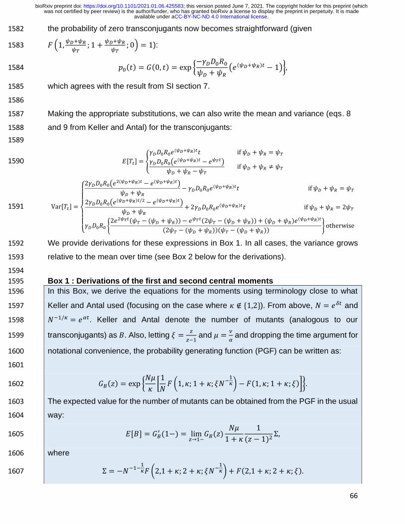
66
the probability of zero transconjugants now becomes straightforward (given 1582
𝐹 (1,𝜓𝐷+𝜓𝑅
𝜓𝑇; 1 +
𝜓𝐷+𝜓𝑅
𝜓𝑇; 0) = 1): 1583
𝑝0(𝑡) = 𝐺(0, 𝑡) = exp {−𝛾𝐷𝐷0𝑅0𝜓𝐷 + 𝜓𝑅
(𝑒(𝜓𝐷+𝜓𝑅)𝑡 − 1)}, 1584
which agrees with the result from SI section 7. 1585
1586
Making the appropriate substitutions, we can also write the mean and variance (eqs. 8 1587
and 9 from Keller and Antal) for the transconjugants: 1588
1589
𝐸[𝑇𝑡] = {
𝛾𝐷𝐷0𝑅0𝑒(𝜓𝐷+𝜓𝑅)𝑡𝑡 if 𝜓𝐷 + 𝜓𝑅 = 𝜓𝑇
𝛾𝐷𝐷0𝑅0(𝑒(𝜓𝐷+𝜓𝑅)𝑡 − 𝑒𝜓𝑇𝑡)
𝜓𝐷 + 𝜓𝑅 −𝜓𝑇 if 𝜓𝐷 + 𝜓𝑅 ≠ 𝜓𝑇
1590
Var[𝑇𝑡] =
{
2𝛾𝐷𝐷0𝑅0(𝑒
2(𝜓𝐷+𝜓𝑅)𝑡 − 𝑒(𝜓𝐷+𝜓𝑅)𝑡)
𝜓𝐷 + 𝜓𝑅− 𝛾𝐷𝐷0𝑅0𝑒
(𝜓𝐷+𝜓𝑅)𝑡𝑡 if 𝜓𝐷 +𝜓𝑅 = 𝜓𝑇
2𝛾𝐷𝐷0𝑅0(𝑒(𝜓𝐷+𝜓𝑅)𝑡/2 − 𝑒(𝜓𝐷+𝜓𝑅)𝑡)
𝜓𝐷 + 𝜓𝑅+ 2𝛾𝐷𝐷0𝑅0𝑒
(𝜓𝐷+𝜓𝑅)𝑡𝑡 if 𝜓𝐷 + 𝜓𝑅 = 2𝜓𝑇
𝛾𝐷𝐷0𝑅0 {2𝑒2𝜓𝑇𝑡(𝜓𝑇 − (𝜓𝐷 + 𝜓𝑅)) − 𝑒
𝜓𝑇𝑡(2𝜓𝑇 − (𝜓𝐷 + 𝜓𝑅)) + (𝜓𝐷 + 𝜓𝑅)𝑒(𝜓𝐷+𝜓𝑅)𝑡
(2𝜓𝑇 − (𝜓𝐷 + 𝜓𝑅))(𝜓𝑇 − (𝜓𝐷 +𝜓𝑅))} otherwise
1591
We provide derivations for these expressions in Box 1. In all cases, the variance grows 1592
relative to the mean over time (see Box 2 below for the derivations). 1593
1594
Box 1 : Derivations of the first and second central moments 1595
In this Box, we derive the equations for the moments using terminology close to what 1596
Keller and Antal used (focusing on the case where 𝜅 ∉ {1,2}). From above, 𝑁 = 𝑒𝛿𝑡 and 1597
𝑁−1/𝜅 = 𝑒𝛼𝑡. Keller and Antal denote the number of mutants (analogous to our 1598
transconjugants) as 𝐵. Also, letting 𝜉 =𝑧
𝑧−1 and 𝜇 =
𝜈
𝛼 and dropping the time argument for 1599
notational convenience, the probability generating function (PGF) can be written as: 1600
1601
𝐺𝐵(𝑧) = exp {𝑁𝜇
𝜅[1
𝑁𝐹 (1, 𝜅; 1 + 𝜅; 𝜉𝑁−
1𝜅) − 𝐹(1, 𝜅; 1 + 𝜅; 𝜉)]}. 1602
The expected value for the number of mutants can be obtained from the PGF in the usual 1603
way: 1604
𝐸[𝐵] = 𝐺𝐵′ (1−) = lim
𝑧→1−𝐺𝐵(𝑧)
𝑁𝜇
1 + 𝜅
1
(𝑧 − 1)2Σ, 1605
where 1606
Σ = −𝑁−1−1𝜅𝐹 (2,1 + 𝜅; 2 + 𝜅; 𝜉𝑁−
1𝜅) + 𝐹(2,1 + 𝜅; 2 + 𝜅; 𝜉). 1607
.CC-BY-NC-ND 4.0 International licenseavailable under awas not certified by peer review) is the author/funder, who has granted bioRxiv a license to display the preprint in perpetuity. It is made
The copyright holder for this preprint (whichthis version posted June 7, 2021. ; https://doi.org/10.1101/2021.01.06.425583doi: bioRxiv preprint

67
We use the following identity 1608
𝐹(𝑎, 𝑏; 𝑐; 𝑧) = (1 − 𝑧)𝑐−𝑎−𝑏𝐹(𝑐 − 𝑎, 𝑐 − 𝑏; 𝑐; 𝑧), 1609
to obtain 1610
𝐹(2,1 + 𝜅; 2 + 𝜅; 𝜉) = (1 − 𝜉)−1𝐹(𝜅, 1,2 + 𝜅, 𝜉) 1611
= (1 − 𝑧)𝐹 (𝜅, 1,2 + 𝜅,𝑧
𝑧 − 1) 1612
Using a related identity 1613
𝐹(𝑎, 𝑏; 𝑐; 𝑧) = (1 − 𝑧)−𝑏𝐹 (𝑐 − 𝑎, 𝑏; 𝑐;𝑧
𝑧 − 1), 1614
we get: 1615
𝐹(2,1 + 𝜅; 2 + 𝜅; 𝜉) = (1 − 𝑧)𝐹 (𝜅, 1,2 + 𝜅,𝑧
𝑧 − 1) 1616
= (1 − 𝑧)2𝐹(2,1,2 + 𝜅, 𝑧) 1617
We will use a similar procedure for the first term in Σ, obtaining: 1618
𝐹(2,1 + 𝜅; 2 + 𝜅; 𝜉𝑁−1/𝜅) = (1 − 𝜉𝑁−1/𝜅)−1𝐹(𝜅, 1,2 + 𝜅; 𝜉𝑁−1/𝜅) 1619
= (1 − 𝜉𝑁−1/𝜅)−1𝐹 (𝜅, 1,2 + 𝜅;𝑥
𝑥 − 1) 1620
= (1 − 𝜉𝑁−1/𝜅)−1(1 − 𝑥)𝐹(2,1,2 + 𝜅; 𝑥) 1621
=(𝑧 − 1)2
(𝑧𝑁−1/𝜅 − 𝑧 + 1)2𝐹(2,1; 2 + 𝜅; 𝑥) 1622
where 𝑥 =𝑧𝑁−1/𝜅
𝑧𝑁−1/𝜅−𝑧+1. 1623
In sum, we have shown that the first derivative of the PGF can be expressed in the 1624
following way: 1625
𝐺𝐵′ (𝑧) = 𝐺𝐵(𝑧)
𝑁𝜇
1 + 𝜅(−
𝑁−1−1𝜅
(𝑧𝑁−1𝜅 − 𝑧 + 1)2
𝐹(2,1;2 + 𝜅; 𝑥) + 𝐹(2,1,2 + 𝜅, 𝑧)). [B1.1] 1626
Using the fact that lim𝑧→1−
𝐺𝐵(𝑧) = 1 and the Gauss identity 𝐹(𝑎, 𝑏; 𝑐; 1) =Γ(𝑐)Γ(𝑐−𝑎−𝑏)
Γ(𝑐−𝑎)Γ(𝑐−𝑏) (which 1627
holds if 𝑐 > 𝑎 + 𝑏) we obtain 1628
𝐸[𝐵] = 𝐺𝐵′ (1−) =
𝑁𝜇
𝜅 − 1(−𝑁−1+1/𝜅 + 1). 1629
To calculate the variance for the number of mutants, we note that 1630
𝐺𝐵″(1−) = 𝐸[𝐵2] − 𝐸[𝐵], 1631
and thus 1632
Var[𝐵] = 𝐺𝐵″(1−) + 𝐸[𝐵] − (𝐸[𝐵])2 1633
= 𝐺𝐵″(1−) + 𝐺𝐵
′ (1−) − (𝐺𝐵′ (1−))2 1634
.CC-BY-NC-ND 4.0 International licenseavailable under awas not certified by peer review) is the author/funder, who has granted bioRxiv a license to display the preprint in perpetuity. It is made
The copyright holder for this preprint (whichthis version posted June 7, 2021. ; https://doi.org/10.1101/2021.01.06.425583doi: bioRxiv preprint

68
From equation [B1.1] we can express the first derivative of the PGF as: 1635
𝐺𝐵′ (𝑧) = 𝐺𝐵(𝑧)
𝑁𝜇
1 + 𝜅Σ1. 1636
It follows that 1637
Var[𝐵] = 𝐺𝐵″(1−)+ 𝐺𝐵
′ (1−) − (𝐺𝐵′ (1−))2 1638
=𝑁𝜇
1 + 𝜅lim𝑧→1−
(Σ1 + Σ1′ ) 1639
= 𝐸[𝐵] +𝑁𝜇
1 + 𝜅lim𝑧→1−
Σ1′ 1640
To calculate the derivative of Σ1, we note that 1641
Σ1 = −𝑁−1−
1𝜅
(𝑧𝑁−1𝜅 − 𝑧 + 1)2
𝐹(2,1; 2 + 𝜅; 𝑥) + 𝐹(2,1,2 + 𝜅, 𝑧). 1642
We can calculate the derivative of the second term: 1643
∂𝐹(2,1,2 + 𝜅, 𝑧)
∂𝑧=
2
2 + 𝜅𝐹(3,2; 3 + 𝜅; 𝑧), 1644
and of the first term: 1645
∂[−𝑁−1−1/𝜅
(𝑧𝑁−1/𝜅 − 𝑧 + 1)2𝐹(2,1; 2 + 𝜅; 𝑥)]
∂𝑧1646
= −𝑁−1−1/𝜅 (−2(𝑁−1/𝜅 − 1)
(𝑁−1/𝜅𝑧 − 𝑧 + 1)3𝐹(2,1; 2 + 𝜅; 𝑥)1647
+2𝑁−1/𝜅
(𝑁−1/𝜅𝑧 − 𝑧 + 1)41
2 + 𝜅𝐹(3,2;3 + 𝜅; 𝑥)) 1648
Taken together, and using Gauss' equality, 1649
lim𝑧→1−
Σ1′ = 2(𝑁−1+1/𝜅 − 𝑁−1+2/𝜅)
𝜅 + 1
𝜅 − 1+
2
2 + 𝜅
(𝜅 + 2)(𝜅 + 1)
(𝜅 − 1)(𝜅 − 2)(1 − 𝑁−1+2/𝜅) 1650
= 2𝑁−1+2/𝜅𝜅 + 1
𝜅 − 1(−1 −
1
𝜅 − 2) + 2𝑁−1+1/𝜅
𝜅 + 1
𝜅 − 1+
2(𝜅 + 1)
(𝜅 − 1)(𝜅 − 2) 1651
= 2𝑁−1+2/𝜅𝜅 + 1
2 − 𝜅+ 2𝑁−1+1/𝜅
𝜅 + 1
𝜅 − 1+
2(𝜅 + 1)
(𝜅 − 1)(𝜅 − 2) 1652
Coming back to 1653
Var[𝐵] = 𝐸[𝐵] +𝑁𝜇
1 + 𝜅lim𝑧→1−
Σ1′ , 1654
we obtain 1655
Var[𝐵] = 𝑁𝜇 [2
2 − 𝜅𝑁−1+
2𝜅 +
1
𝜅 − 1𝑁−1+
1𝜅 +
𝜅
(𝜅 − 1)(𝜅 − 2)]. 1656
.CC-BY-NC-ND 4.0 International licenseavailable under awas not certified by peer review) is the author/funder, who has granted bioRxiv a license to display the preprint in perpetuity. It is made
The copyright holder for this preprint (whichthis version posted June 7, 2021. ; https://doi.org/10.1101/2021.01.06.425583doi: bioRxiv preprint

69
Making the appropriate substitutions yields our expressions for the mean and variance 1657
for our transconjugants. 1658
1659
Box 2 : Behavior of the variance relative to the mean over time 1660
In this Box, we will show that the variance in transconjugant numbers grows relative to 1661
the mean over time. To do so, we will need to consider several cases. 1662
1663
Let’s consider the ratio of the variance to the mean, which we denote 𝜌𝑡 =Var[𝑇𝑡]
𝐸[𝑇𝑡]. We will 1664
start by focusing on the case where 𝜓𝐷 + 𝜓𝑅 ≠ 𝜓𝑇 and 𝜓𝐷 +𝜓𝑅 ≠ 2𝜓𝑇: 1665
𝜌𝑡 =𝛾𝐷𝐷0𝑅0 {
2𝑒2𝜓𝑇𝑡(𝜓𝑇 − (𝜓𝐷 + 𝜓𝑅)) − 𝑒𝜓𝑇𝑡(2𝜓𝑇 − (𝜓𝐷 + 𝜓𝑅)) + (𝜓𝐷 +𝜓𝑅)𝑒
(𝜓𝐷+𝜓𝑅)𝑡
(2𝜓𝑇 − (𝜓𝐷 + 𝜓𝑅))(𝜓𝑇 − (𝜓𝐷 + 𝜓𝑅))}
𝛾𝐷𝐷0𝑅0(𝑒(𝜓𝐷+𝜓𝑅)𝑡 − 𝑒𝜓𝑇𝑡)𝜓𝐷 +𝜓𝑅 − 𝜓𝑇
. 1666
This can be simplified as follows: 1667
𝜌𝑡 =2𝑒2𝜓𝑇𝑡(𝜓𝑇 − (𝜓𝐷 + 𝜓𝑅)) − 𝑒
𝜓𝑇𝑡(2𝜓𝑇 − (𝜓𝐷 + 𝜓𝑅)) + (𝜓𝐷 +𝜓𝑅)𝑒(𝜓𝐷+𝜓𝑅)𝑡
(𝜓𝐷 +𝜓𝑅 − 2𝜓𝑇)(𝑒(𝜓𝐷+𝜓𝑅)𝑡 − 𝑒𝜓𝑇𝑡). 1668
Letting 𝜅 =𝜓𝐷+𝜓𝑅
𝜓𝑇, 1669
𝜌𝑡 =2𝑒2𝜓𝑇𝑡(1 − 𝜅) − 𝑒𝜓𝑇𝑡(2 − 𝜅) + 𝜅𝑒(𝜓𝐷+𝜓𝑅)𝑡
(𝜅 − 2)(𝑒(𝜓𝐷+𝜓𝑅)𝑡 − 𝑒𝜓𝑇𝑡), 1670
𝜌𝑡 =𝜅𝑒(𝜓𝐷+𝜓𝑅)𝑡 − 2(𝜅 − 1)𝑒2𝜓𝑇𝑡 + (𝜅 − 2)𝑒𝜓𝑇𝑡
(𝜅 − 2)(𝑒(𝜓𝐷+𝜓𝑅)𝑡 − 𝑒𝜓𝑇𝑡). 1671
To determine the behavior of this ratio over time we take the derivative with respect to 1672
time: 1673
𝑑𝜌𝑡𝑑𝑡
1674
=
{(𝜅(𝜓𝐷 +𝜓𝑅)𝑒
(𝜓𝐷+𝜓𝑅)𝑡 − 4𝜓𝑇(𝜅 − 1)𝑒2𝜓𝑇𝑡 + (𝜅 − 2)𝜓𝑇𝑒
𝜓𝑇𝑡)(𝜅 − 2)(𝑒(𝜓𝐷+𝜓𝑅)𝑡 − 𝑒𝜓𝑇𝑡)
−(𝜅𝑒(𝜓𝐷+𝜓𝑅)𝑡 − 2(𝜅 − 1)𝑒2𝜓𝑇𝑡 + (𝜅 − 2)𝑒𝜓𝑇𝑡)(𝜅 − 2) ((𝜓𝐷 +𝜓𝑅)𝑒(𝜓𝐷+𝜓𝑅)𝑡 − 𝜓𝑇𝑒
𝜓𝑇𝑡)}
((𝜅 − 2)(𝑒(𝜓𝐷+𝜓𝑅)𝑡 − 𝑒𝜓𝑇𝑡))2 1675
𝑑𝜌𝑡𝑑𝑡
={
(𝜅(𝜓𝐷 + 𝜓𝑅)𝑒
(𝜓𝐷+𝜓𝑅)𝑡 − 4𝜓𝑇(𝜅 − 1)𝑒2𝜓𝑇𝑡 + (𝜅 − 2)𝜓𝑇𝑒
𝜓𝑇𝑡)(𝜅 − 2)(𝑒(𝜓𝐷+𝜓𝑅)𝑡)
−(𝜅(𝜓𝐷 +𝜓𝑅)𝑒(𝜓𝐷+𝜓𝑅)𝑡 − 4𝜓𝑇(𝜅 − 1)𝑒
2𝜓𝑇𝑡 + (𝜅 − 2)𝜓𝑇𝑒𝜓𝑇𝑡)(𝜅 − 2)(𝑒𝜓𝑇𝑡)
−(𝜅𝑒(𝜓𝐷+𝜓𝑅)𝑡 − 2(𝜅 − 1)𝑒2𝜓𝑇𝑡 + (𝜅 − 2)𝑒𝜓𝑇𝑡)(𝜅 − 2) ((𝜓𝐷 + 𝜓𝑅)𝑒(𝜓𝐷+𝜓𝑅)𝑡)
+(𝜅𝑒(𝜓𝐷+𝜓𝑅)𝑡 − 2(𝜅 − 1)𝑒2𝜓𝑇𝑡 + (𝜅 − 2)𝑒𝜓𝑇𝑡)(𝜅 − 2)(𝜓𝑇𝑒𝜓𝑇𝑡) }
((𝜅 − 2)(𝑒(𝜓𝐷+𝜓𝑅)𝑡 − 𝑒𝜓𝑇𝑡))2 , 1676
.CC-BY-NC-ND 4.0 International licenseavailable under awas not certified by peer review) is the author/funder, who has granted bioRxiv a license to display the preprint in perpetuity. It is made
The copyright holder for this preprint (whichthis version posted June 7, 2021. ; https://doi.org/10.1101/2021.01.06.425583doi: bioRxiv preprint

70
𝑑𝜌𝑡𝑑𝑡
={
(−4𝜓𝑇(𝜅 − 1)𝑒2𝜓𝑇𝑡 + (𝜅 − 2)𝜓𝑇𝑒
𝜓𝑇𝑡)(𝜅 − 2)(𝑒(𝜓𝐷+𝜓𝑅)𝑡)
−(𝜅(𝜓𝐷 + 𝜓𝑅)𝑒(𝜓𝐷+𝜓𝑅)𝑡 − 4𝜓𝑇(𝜅 − 1)𝑒
2𝜓𝑇𝑡)(𝜅 − 2)(𝑒𝜓𝑇𝑡)
−(−2(𝜅 − 1)𝑒2𝜓𝑇𝑡 + (𝜅 − 2)𝑒𝜓𝑇𝑡)(𝜅 − 2)((𝜓𝐷 +𝜓𝑅)𝑒(𝜓𝐷+𝜓𝑅)𝑡)
+(𝜅𝑒(𝜓𝐷+𝜓𝑅)𝑡 − 2(𝜅 − 1)𝑒2𝜓𝑇𝑡)(𝜅 − 2)(𝜓𝑇𝑒𝜓𝑇𝑡) }
((𝜅 − 2)(𝑒(𝜓𝐷+𝜓𝑅)𝑡 − 𝑒𝜓𝑇𝑡))2 , 1677
𝑑𝜌𝑡𝑑𝑡
={
(𝜓𝐷 + 𝜓𝑅 − 2𝜓𝑇)2(𝜅 − 1)(𝜅 − 2)𝑒
2𝜓𝑇𝑡(𝑒(𝜓𝐷+𝜓𝑅)𝑡)
−(𝜓𝐷 + 𝜓𝑅 −𝜓𝑇)(𝜅 − 2)2𝑒𝜓𝑇𝑡(𝑒(𝜓𝐷+𝜓𝑅)𝑡)
−(𝜓𝐷 +𝜓𝑅 −𝜓𝑇)𝜅(𝜅 − 2)𝑒𝜓𝑇𝑡(𝑒(𝜓𝐷+𝜓𝑅)𝑡)
+2𝜓𝑇(𝜅 − 1)(𝜅 − 2)𝑒3𝜓𝑇𝑡 }
((𝜅 − 2)(𝑒(𝜓𝐷+𝜓𝑅)𝑡 − 𝑒𝜓𝑇𝑡))2 , 1678
𝑑𝜌𝑡𝑑𝑡
=
{
(𝜓𝐷 + 𝜓𝑅 − 2𝜓𝑇)2(𝜅 − 1)(𝜅 − 2)𝑒2𝜓𝑇𝑡(𝑒(𝜓𝐷+𝜓𝑅)𝑡)
−(𝜓𝐷 + 𝜓𝑅 −𝜓𝑇)2(𝜅 − 1)(𝜅 − 2)𝑒𝜓𝑇𝑡(𝑒(𝜓𝐷+𝜓𝑅)𝑡)
+2𝜓𝑇(𝜅 − 1)(𝜅 − 2)𝑒3𝜓𝑇𝑡
}
((𝜅 − 2)(𝑒(𝜓𝐷+𝜓𝑅)𝑡 − 𝑒𝜓𝑇𝑡))2 , 1679
𝑑𝜌𝑡𝑑𝑡
=(𝜅 − 1)(𝜅 − 2){(𝜅 − 2)𝑒(𝜓𝐷+𝜓𝑅+2𝜓𝑇)𝑡 − (𝜅 − 1)𝑒(𝜓𝐷+𝜓𝑅+𝜓𝑇)𝑡 + 𝑒3𝜓𝑇𝑡}
(12𝜓𝑇
) ((𝜅 − 2)(𝑒(𝜓𝐷+𝜓𝑅)𝑡 − 𝑒𝜓𝑇𝑡))2
, 1680
𝑑𝜌𝑡𝑑𝑡
=(𝜅 − 1)(𝜅 − 2)𝑒𝜓𝑇𝑡{(𝜅 − 2)𝑒(𝜓𝐷+𝜓𝑅+𝜓𝑇)𝑡 − (𝜅 − 1)𝑒(𝜓𝐷+𝜓𝑅)𝑡 + 𝑒2𝜓𝑇𝑡}
(12𝜓𝑇
) ((𝜅 − 2)(𝑒(𝜓𝐷+𝜓𝑅)𝑡 − 𝑒𝜓𝑇𝑡))2
, 1681
𝑑𝜌𝑡𝑑𝑡
=(𝜅 − 1)(𝜅 − 2){(𝜅 − 2)𝑒(𝜅+1)𝜓𝑇𝑡 − (𝜅 − 1)𝑒𝜅𝜓𝑇𝑡 + 𝑒2𝜓𝑇𝑡}
(𝑒−𝜓𝑇𝑡
2𝜓𝑇) ((𝜅 − 2)(𝑒(𝜓𝐷+𝜓𝑅)𝑡 − 𝑒𝜓𝑇𝑡))
2. 1682
The denominator is always positive, so the sign of this derivative is governed by the 1683
numerator 1684
sign [𝑑𝜌𝑡𝑑𝑡] = sign[(𝜅 − 1)(𝜅 − 2){(𝜅 − 2)𝑒(𝜅+1)𝜓𝑇𝑡 − (𝜅 − 1)𝑒𝜅𝜓𝑇𝑡 + 𝑒2𝜓𝑇𝑡}]. 1685
For 𝜅 > 2, which is when the growth rate of the transconjugant is less than the average 1686
of the donor and recipient growth rates, we have 1687
sign [𝑑𝜌𝑡𝑑𝑡] = sign[(𝜅 − 2)𝑒(𝜅+1)𝜓𝑇𝑡 − (𝜅 − 1)𝑒𝜅𝜓𝑇𝑡 + 𝑒2𝜓𝑇𝑡]. 1688
For any 𝑡 > 0, for 𝜅 = 2 1689
sign [𝑑𝜌𝑡𝑑𝑡] = sign[0 − 𝑒2𝜓𝑇𝑡 + 𝑒2𝜓𝑇𝑡] = 0. 1690
Now letting 𝑔(𝜅) = (𝜅 − 2)𝑒(𝜅+1)𝜓𝑇𝑡 − (𝜅 − 1)𝑒𝜅𝜓𝑇𝑡 + 𝑒2𝜓𝑇𝑡, we have 1691
𝑔′(𝜅) = 𝑒(𝜅+1)𝜓𝑇𝑡 + (𝜅 − 2)𝜓𝑇𝑡𝑒(𝜅+1)𝜓𝑇𝑡 − 𝑒𝜅𝜓𝑇𝑡 − (𝜅 − 1)𝜓𝑇𝑡𝑒
𝜅𝜓𝑇𝑡 , 1692
.CC-BY-NC-ND 4.0 International licenseavailable under awas not certified by peer review) is the author/funder, who has granted bioRxiv a license to display the preprint in perpetuity. It is made
The copyright holder for this preprint (whichthis version posted June 7, 2021. ; https://doi.org/10.1101/2021.01.06.425583doi: bioRxiv preprint

71
𝑔′(𝜅) = {1 + (𝜅 − 2)𝜓𝑇𝑡}𝑒(𝜅+1)𝜓𝑇𝑡 − {1 + (𝜅 − 1)𝜓𝑇𝑡}𝑒
𝜅𝜓𝑇𝑡 . 1693
Letting ℎ(𝑥) = {1 + (𝜅 − 1 − 𝑥)𝜓𝑇𝑡}𝑒(𝜅+𝑥)𝜓𝑇𝑡, we see 1694
𝑔′(𝜅) = ℎ(1) − ℎ(0). 1695
But we see that 1696
ℎ′(𝑥) = −𝜓𝑇𝑡𝑒(𝜅+𝑥)𝜓𝑇𝑡 + {1 + (𝜅 − 1 − 𝑥)𝜓𝑇𝑡}𝜓𝑇𝑡𝑒
(𝜅+𝑥)𝜓𝑇𝑡 , 1697
ℎ′(𝑥) = 𝜓𝑇𝑡𝑒(𝜅+𝑥)𝜓𝑇𝑡(−1 + {1 + (𝜅 − 1 − 𝑥)𝜓𝑇𝑡}), 1698
ℎ′(𝑥) = 𝜓𝑇𝑡𝑒(𝜅+𝑥)𝜓𝑇𝑡(𝜅 − 1 − 𝑥)𝜓𝑇𝑡. 1699
If 𝜅 > 2 and 𝑡 > 0, then ℎ′(𝑥) > 0 for 0 ≤ 𝑥 ≤ 1. Since ℎ(𝑥) is a continuous function, we 1700
must have 1701
ℎ(1) > ℎ(0). 1702
This implies that for 𝜅 > 2 and 𝑡 > 0, 1703
𝑔′(𝜅) > 0. 1704
Since 𝑔(𝜅) is also continuous, and since 𝑔(2) = 0, we now know that for 𝜅 > 2 and 𝑡 >1705
0, 1706
𝑔(𝜅) > 0. 1707
Therefore sign [𝑑𝜌𝑡
𝑑𝑡] = 1, or the derivative is positive for 𝑡 > 0 and 𝜅 > 2, which means 1708
the variance grows relative to the mean over time. 1709
For 1 < 𝜅 < 2, 1710
sign [𝑑𝜌𝑡𝑑𝑡] = sign[−(𝜅 − 2)𝑒(𝜅+1)𝜓𝑇𝑡 + (𝜅 − 1)𝑒𝜅𝜓𝑇𝑡 − 𝑒2𝜓𝑇𝑡]. 1711
Letting 𝜑 = −(𝜅 − 2), we know that 0 < 𝜑 < 1, and we can rewrite the above 1712
sign [𝑑𝜌𝑡𝑑𝑡] = sign[𝜑𝑒(3−𝜑)𝜓𝑇𝑡 + (1 − 𝜑)𝑒(3−(1+𝜑))𝜓𝑇𝑡 − 𝑒2𝜓𝑇𝑡]. 1713
Because 𝑒(3−𝑥)𝜓𝑇𝑡 is convex (𝑡 > 0 ⟹𝑑2𝑒(3−𝑥)𝜓𝑇𝑡
𝑑𝑥2> 0), Jensen’s inequality ensures 1714
𝜑𝑒(3−𝜑)𝜓𝑇𝑡 + (1 − 𝜑)𝑒(3−(1+𝜑))𝜓𝑇𝑡 − 𝑒2𝜓𝑇𝑡 > 𝑒(3−(𝜑2+(1−𝜑)(1+𝜑)))𝜓𝑇𝑡 − 𝑒2𝜓𝑇𝑡 , 1715
𝜑𝑒(3−𝜑)𝜓𝑇𝑡 + (1 − 𝜑)𝑒(3−(1+𝜑))𝜓𝑇𝑡 − 𝑒2𝜓𝑇𝑡 > 𝑒(3−(𝜑2+1−𝜑2))𝜓𝑇𝑡 − 𝑒2𝜓𝑇𝑡 , 1716
𝜑𝑒(3−𝜑)𝜓𝑇𝑡 + (1 − 𝜑)𝑒(3−(1+𝜑))𝜓𝑇𝑡 − 𝑒2𝜓𝑇𝑡 > 𝑒2𝜓𝑇𝑡 − 𝑒2𝜓𝑇𝑡 , 1717
𝜑𝑒(3−𝜑)𝜓𝑇𝑡 + (1 − 𝜑)𝑒(3−(1+𝜑))𝜓𝑇𝑡 − 𝑒2𝜓𝑇𝑡 > 0. 1718
Therefore sign [𝑑𝜌𝑡
𝑑𝑡] = 1, or the derivative is positive for 𝑡 > 0 and 1 < 𝜅 < 2, which 1719
means the variance grows relative to the mean over time. 1720
1721
Next, we turn to 0 < 𝜅 < 1, where 1722
.CC-BY-NC-ND 4.0 International licenseavailable under awas not certified by peer review) is the author/funder, who has granted bioRxiv a license to display the preprint in perpetuity. It is made
The copyright holder for this preprint (whichthis version posted June 7, 2021. ; https://doi.org/10.1101/2021.01.06.425583doi: bioRxiv preprint

72
sign [𝑑𝜌𝑡𝑑𝑡] = sign[(𝜅 − 2)𝑒(𝜅+1)𝜓𝑇𝑡 − (𝜅 − 1)𝑒𝜅𝜓𝑇𝑡 + 𝑒2𝜓𝑇𝑡]. 1723
For any 𝑡 > 0, for 𝜅 = 1 1724
sign [𝑑𝜌𝑡𝑑𝑡] = sign[−𝑒2𝜓𝑇𝑡 − 0 + 𝑒2𝜓𝑇𝑡] = 0. 1725
Now letting 𝑔(𝜅) = (𝜅 − 2)𝑒(𝜅+1)𝜓𝑇𝑡 − (𝜅 − 1)𝑒𝜅𝜓𝑇𝑡 + 𝑒2𝜓𝑇𝑡, we have from above 1726
𝑔′(𝜅) = {1 + (𝜅 − 2)𝜓𝑇𝑡}𝑒(𝜅+1)𝜓𝑇𝑡 − {1 + (𝜅 − 1)𝜓𝑇𝑡}𝑒
𝜅𝜓𝑇𝑡 . 1727
Letting ℎ(𝑥) = {1 + (𝜅 − 1 − 𝑥)𝜓𝑇𝑡}𝑒(𝜅+𝑥)𝜓𝑇𝑡, we see 1728
𝑔′(𝜅) = ℎ(1) − ℎ(0). 1729
But we see from above that 1730
ℎ′(𝑥) = 𝜓𝑇𝑡𝑒(𝜅+𝑥)𝜓𝑇𝑡(𝜅 − 1 − 𝑥)𝜓𝑇𝑡. 1731
If 0 < 𝜅 < 1 and 𝑡 > 0, then ℎ′(𝑥) < 0 for 0 ≤ 𝑥 ≤ 1. Since ℎ(𝑥) is a continuous function, 1732
we must have 1733
ℎ(1) < ℎ(0). 1734
This implies that for 0 < 𝜅 < 1 and 𝑡 > 0, 1735
𝑔′(𝜅) < 0. 1736
Since 𝑔(𝜅) is continuous, and since 𝑔(1) = 0, we now know that for 0 < 𝜅 < 1 and 𝑡 >1737
0, 𝑔(𝜅) > 0. Therefore sign [𝑑𝜌𝑡
𝑑𝑡] = 1, or the derivative is positive for 𝑡 > 0 and 0 < 𝜅 < 1, 1738
which means the variance grows relative to the mean over time. 1739
1740
Now consider the special case of 𝜅 = 2 1741
𝜌𝑡 =
2𝛾𝐷𝐷0𝑅0(𝑒𝜓𝑇𝑡 − 𝑒2𝜓𝑇𝑡)2𝜓𝑇
+ 2𝛾𝐷𝐷0𝑅0𝑒2𝜓𝑇𝑡𝑡
𝛾𝐷𝐷0𝑅0(𝑒2𝜓𝑇𝑡 − 𝑒𝜓𝑇𝑡)
2𝜓𝑇 − 𝜓𝑇
, 1742
𝜌𝑡 =(𝑒𝜓𝑇𝑡 − 𝑒2𝜓𝑇𝑡) + 2𝜓𝑇𝑡𝑒
2𝜓𝑇𝑡
(𝑒2𝜓𝑇𝑡 − 𝑒𝜓𝑇𝑡), 1743
𝜌𝑡 =(2𝜓𝑇𝑡 − 1)𝑒
2𝜓𝑇𝑡 + 𝑒𝜓𝑇𝑡
(𝑒2𝜓𝑇𝑡 − 𝑒𝜓𝑇𝑡). 1744
Taking the derivative with respect to time yields 1745
𝑑𝜌𝑡𝑑𝑡
=
{(2𝜓𝑇𝑒
2𝜓𝑇𝑡 + 2𝜓𝑇(2𝜓𝑇𝑡 − 1)𝑒2𝜓𝑇𝑡 + 𝜓𝑇𝑒
𝜓𝑇𝑡)(𝑒2𝜓𝑇𝑡 − 𝑒𝜓𝑇𝑡)
− ((2𝜓𝑇𝑡 − 1)𝑒2𝜓𝑇𝑡 + 𝑒𝜓𝑇𝑡) (2𝜓𝑇𝑒
2𝜓𝑇𝑡 − 𝜓𝑇𝑒𝜓𝑇𝑡)
}
(𝑒2𝜓𝑇𝑡 − 𝑒𝜓𝑇𝑡)2, 1746
𝑑𝜌𝑡𝑑𝑡
= 𝜓𝑇(4𝜓𝑇𝑡𝑒
2𝜓𝑇𝑡 + 𝑒𝜓𝑇𝑡)(𝑒2𝜓𝑇𝑡 − 𝑒𝜓𝑇𝑡) − ((2𝜓𝑇𝑡 − 1)𝑒2𝜓𝑇𝑡 + 𝑒𝜓𝑇𝑡) (2𝑒2𝜓𝑇𝑡 − 𝑒𝜓𝑇𝑡)
(𝑒2𝜓𝑇𝑡 − 𝑒𝜓𝑇𝑡)2, 1747
.CC-BY-NC-ND 4.0 International licenseavailable under awas not certified by peer review) is the author/funder, who has granted bioRxiv a license to display the preprint in perpetuity. It is made
The copyright holder for this preprint (whichthis version posted June 7, 2021. ; https://doi.org/10.1101/2021.01.06.425583doi: bioRxiv preprint

73
𝑑𝜌𝑡𝑑𝑡
= 𝜓𝑇
{4𝜓𝑇𝑡𝑒
4𝜓𝑇𝑡 + 𝑒3𝜓𝑇𝑡 − 4𝜓𝑇𝑡𝑒3𝜓𝑇𝑡 − 𝑒2𝜓𝑇𝑡
−2(2𝜓𝑇𝑡 − 1)𝑒4𝜓𝑇𝑡 − 2𝑒3𝜓𝑇𝑡 + (2𝜓𝑇𝑡 − 1)𝑒
3𝜓𝑇𝑡 + 𝑒2𝜓𝑇𝑡}
(𝑒2𝜓𝑇𝑡 − 𝑒𝜓𝑇𝑡)2, 1748
𝑑𝜌𝑡𝑑𝑡
= 𝜓𝑇{4𝜓𝑇𝑡 − 2(2𝜓𝑇𝑡 − 1)}𝑒
4𝜓𝑇𝑡 − {4𝜓𝑇𝑡 + 1 − (2𝜓𝑇𝑡 − 1)}𝑒3𝜓𝑇𝑡
(𝑒2𝜓𝑇𝑡 − 𝑒𝜓𝑇𝑡)2, 1749
𝑑𝜌𝑡𝑑𝑡
= 𝜓𝑇2𝑒4𝜓𝑇𝑡 − {2𝜓𝑇𝑡 + 2}𝑒
3𝜓𝑇𝑡
(𝑒2𝜓𝑇𝑡 − 𝑒𝜓𝑇𝑡)2, 1750
𝑑𝜌𝑡𝑑𝑡
= 2𝜓𝑇𝑒3𝜓𝑇𝑡
𝑒𝜓𝑇𝑡 −𝜓𝑇𝑡 − 1
(𝑒2𝜓𝑇𝑡 − 𝑒𝜓𝑇𝑡)2. 1751
Using the Taylor expansion 1752
𝑑𝜌𝑡𝑑𝑡
= 2𝜓𝑇𝑒3𝜓𝑇𝑡
(1 + 𝜓𝑇𝑡 +(𝜓𝑇𝑡)
2
2! +(𝜓𝑇𝑡)
3
3! +(𝜓𝑇𝑡)
4
4! … ) − 𝜓𝑇𝑡 − 1
(𝑒2𝜓𝑇𝑡 − 𝑒𝜓𝑇𝑡)2, 1753
𝑑𝜌𝑡𝑑𝑡
= 2𝜓𝑇𝑒3𝜓𝑇𝑡
((𝜓𝑇𝑡)
2
2! +(𝜓𝑇𝑡)
3
3! +(𝜓𝑇𝑡)
4
4! … )
(𝑒2𝜓𝑇𝑡 − 𝑒𝜓𝑇𝑡)2. 1754
Therefore, 𝑑𝜌𝑡
𝑑𝑡> 0 for 𝑡 > 0 and 𝜅 = 2, which means the variance grows relative to the 1755
mean over time. 1756
1757
Finally, consider the special case of 𝜅 = 1 1758
𝜌𝑡 =
2𝛾𝐷𝐷0𝑅0(𝑒2𝜓𝑇𝑡 − 𝑒𝜓𝑇𝑡)𝜓𝑇
− 𝛾𝐷𝐷0𝑅0𝑒𝜓𝑇𝑡𝑡
𝛾𝐷𝐷0𝑅0𝑒𝜓𝑇𝑡𝑡 , 1759
𝜌𝑡 =2𝑒2𝜓𝑇𝑡 − (2 + 𝜓𝑇𝑡)𝑒
𝜓𝑇𝑡
𝜓𝑇𝑡𝑒𝜓𝑇𝑡 , 1760
𝜌𝑡 =2𝑒𝜓𝑇𝑡 − (2 + 𝜓𝑇𝑡)
𝜓𝑇𝑡 . 1761
Using the Taylor expansion 1762
𝜌𝑡 =2 (1 + 𝜓𝑇𝑡 +
(𝜓𝑇𝑡)2
2! +(𝜓𝑇𝑡)
3
3! +(𝜓𝑇𝑡)
4
4! … ) − (2 + 𝜓𝑇𝑡)
𝜓𝑇𝑡 , 1763
𝜌𝑡 =𝜓𝑇𝑡 + 2(
(𝜓𝑇𝑡)2
2! +(𝜓𝑇𝑡)
3
3! +(𝜓𝑇𝑡)
4
4! … )
𝜓𝑇𝑡 , 1764
𝜌𝑡 = 1 + 2(𝜓𝑇𝑡
2!+(𝜓𝑇𝑡)
2
3!+(𝜓𝑇𝑡)
3
4!…). 1765
Once again, the variance grows relative to the mean over time. 1766
1767
.CC-BY-NC-ND 4.0 International licenseavailable under awas not certified by peer review) is the author/funder, who has granted bioRxiv a license to display the preprint in perpetuity. It is made
The copyright holder for this preprint (whichthis version posted June 7, 2021. ; https://doi.org/10.1101/2021.01.06.425583doi: bioRxiv preprint

74
Overall, we have shown that for all 𝜅 > 0 and 𝑡 > 0, the ratio of the transconjugant 1768
variance to the mean number of transconjugants is amplified over time. 1769
1770
SI section 14 : Variance in Estimates 1771
Here we will focus on two estimates, ASM and LDM, and ask about their variance 1772
(enabling us to compare precision). We will focus exclusively on the contributions to this 1773
variance coming from the stochasticity in the transconjugant numbers (i.e., ignoring 1774
contributions coming from assessment of initial and final donor and recipient populations). 1775
1776
We start with the ASM estimate (here we express the estimate in terms of growth rate 1777
parameters): 1778
𝛾𝐷 =𝜓𝐷 +𝜓𝑅 − 𝜓𝑇
𝐷0𝑅0(𝑒(𝜓𝐷+𝜓𝑅)𝑡 − 𝑒𝜓𝑇𝑡)𝑇𝑡 . 1779
Because we are only focusing on the contribution of the transconjugant variation, all 1780
parameters (initial densities and growth rates will be taken to be fixed). Thus, we can think 1781
about the ASM estimate as a random variable ΓASM, where 1782
ΓASM = 𝑐1𝑇�̃� , 1783
where the constant 𝑐1 is 1784
𝑐1 =𝜓𝐷 +𝜓𝑅 − 𝜓𝑇
𝐷0𝑅0(𝑒(𝜓𝐷+𝜓𝑅)𝑡 − 𝑒𝜓𝑇𝑡)
. 1785
The variance of the ASM estimate is then 1786
var(ΓASM) = 𝑐12{var(𝑇�̃�)}. 1787
But we have a closed form expression for var(𝑇𝑡). If 𝜓𝑇 ∉ {𝜓𝐷 + 𝜓𝑅, (𝜓𝐷 +𝜓𝑅)/2}, we 1788
have: 1789
var(ΓASM) = (𝜓𝐷+𝜓𝑅−𝜓𝑇
𝐷0𝑅0(𝑒(𝜓𝐷+𝜓𝑅)�̃�−𝑒𝜓𝑇�̃�)
)
2
𝛾𝐷𝐷0𝑅0 {
(𝜓𝐷+𝜓𝑅)𝑒(𝜓𝐷+𝜓𝑅)�̃�
(𝜓𝐷+𝜓𝑅−𝜓𝑇)(𝜓𝐷+𝜓𝑅−2𝜓𝑇)+
𝑒𝜓𝑇�̃�
𝜓𝐷+𝜓𝑅−𝜓𝑇−
2𝑒2𝜓𝑇�̃�
𝜓𝐷+𝜓𝑅−2𝜓𝑇}, 1790
var(ΓASM) =𝛾𝐷
𝐷0𝑅0(
𝜓𝐷+𝜓𝑅−𝜓𝑇
𝑒(𝜓𝐷+𝜓𝑅)�̃�−𝑒𝜓𝑇�̃�)2{(𝜓𝐷+𝜓𝑅)𝑒
(𝜓𝐷+𝜓𝑅)�̃�+(𝜓𝐷+𝜓𝑅−2𝜓𝑇)𝑒𝜓𝑇�̃�−(𝜓𝐷+𝜓𝑅−𝜓𝑇)2𝑒
2𝜓𝑇�̃�
(𝜓𝐷+𝜓𝑅−𝜓𝑇)(𝜓𝐷+𝜓𝑅−2𝜓𝑇)}, 1791
var(ΓASM) =𝛾𝐷(𝜓𝐷+𝜓𝑅−𝜓𝑇)
𝐷0𝑅0{(𝜓𝐷+𝜓𝑅)𝑒
(𝜓𝐷+𝜓𝑅)�̃�+(𝜓𝐷+𝜓𝑅−2𝜓𝑇)𝑒𝜓𝑇�̃�−(𝜓𝐷+𝜓𝑅−𝜓𝑇)2𝑒
2𝜓𝑇�̃�
(𝜓𝐷+𝜓𝑅−2𝜓𝑇)(𝑒(𝜓𝐷+𝜓𝑅)�̃�−𝑒𝜓𝑇�̃�)
2 }. 1792
The formulas for 𝜓𝑇 = 𝜓𝐷 + 𝜓𝑅 and 2𝜓𝑇 = 𝜓𝐷 +𝜓𝑅 could also be derived via simple 1793
substitution (note, lim𝜓𝑇→𝜓𝐷+𝜓𝑅
𝑐1 = 1/(𝐷0𝑅0𝑡𝑒(𝜓𝐷+𝜓𝑅)𝑡). These formulas allow us to project 1794
variance in the ASM estimate over time due to transconjugant variation if all parameters 1795
are known. 1796
.CC-BY-NC-ND 4.0 International licenseavailable under awas not certified by peer review) is the author/funder, who has granted bioRxiv a license to display the preprint in perpetuity. It is made
The copyright holder for this preprint (whichthis version posted June 7, 2021. ; https://doi.org/10.1101/2021.01.06.425583doi: bioRxiv preprint

75
1797
We now turn to the LDM estimate: 1798
𝛾𝐷 = − ln �̂�0(�̃�) (𝜓𝐷 +𝜓𝑅
𝐷0𝑅0(𝑒(𝜓𝐷+𝜓𝑅)𝑡 − 1)
). 1799
What we actually measure is the number of populations (or wells) that have no 1800
transconjugants (call this 𝑤) out of the total number of populations (or wells) tracked (call 1801
this W). As we show in SI section 9, the maximum likelihood estimate of 𝑝0(�̃�) is 1802
�̂�0(�̃�) =𝑤
W. 1803
Of course, from experiment to experiment, there will be variance in the number of 1804
populations with no transconjugants. Let us consider a random variable 𝐹, which 1805
represents the fraction of total populations that have no transconjugants. The expectation 1806
of 𝐹 is (we drop the time argument for notational convenience): 1807
E[𝐹] = ∑ (W𝑤) (𝑝0)
𝑤(1 − 𝑝0)W−𝑤 (
𝑤
W)
W
𝑤=0
, 1808
E[𝐹] =1
W∑
W!
𝑤! (W −𝑤)!(𝑝0)
𝑤(1 − 𝑝0)W−𝑤
W
𝑤=1
𝑤, 1809
E[𝐹] =1
W∑
W!
(w − 1)! (W − 𝑤)!(𝑝0)
𝑤(1 − 𝑝0)W−𝑤 ,
W
𝑤=1
1810
E[𝐹] = 𝑝0 ∑(W− 1)!
(w − 1)! ((W− 1) − (w − 1))!(𝑝0)
𝑤−1(1 − 𝑝0)(W−1)−(𝑤−1)
W
𝑤=1
. 1811
Letting 𝑖 = 𝑤 − 1, we have 1812
E[𝐹] = 𝑝0 ∑(W− 1)!
𝑖! ((W − 1) − 𝑖)!(𝑝0)
𝑖(1 − 𝑝0)(W−1)−𝑖
W−1
𝑖=0
. 1813
However, because ∑ (W − 1𝑖
) (𝑝0)𝑖(1 − 𝑝0)
(W−1)−𝑖W−1𝑖=0 = 1, we have 1814
E[𝐹] = 𝑝0, 1815
which makes sense. The second central moment of 𝐹 is 1816
var[𝐹] = ∑ (W𝑤) (𝑝0)
𝑤(1 − 𝑝0)W−𝑤 (
𝑤
W− 𝑝0)
2W
𝑤=0
, 1817
var[𝐹] = ∑ (W𝑤) (𝑝0)
𝑤(1 − 𝑝0)W−𝑤 ((
𝑤
W)2
− 2𝑝0 (𝑤
W) + (𝑝0)
2) ,
W
𝑤=0
1818
.CC-BY-NC-ND 4.0 International licenseavailable under awas not certified by peer review) is the author/funder, who has granted bioRxiv a license to display the preprint in perpetuity. It is made
The copyright holder for this preprint (whichthis version posted June 7, 2021. ; https://doi.org/10.1101/2021.01.06.425583doi: bioRxiv preprint

76
var[𝐹] = ∑ (W𝑤) (𝑝0)
𝑤(1 − 𝑝0)W−𝑤 (
𝑤
W)2
W
𝑤=0
− 2𝑝0 ∑ (W𝑤) (𝑝0)
𝑤(1 − 𝑝0)W−𝑤 (
𝑤
W)
W
𝑤=0
1819
+ (𝑝0)2 ∑ (
W𝑤) (𝑝0)
𝑤(1 − 𝑝0)W−𝑤
W
𝑤=0
, 1820
var[𝐹] = {(1
W2)∑ (
W𝑤) (𝑝0)
𝑤(1 − 𝑝0)W−𝑤𝑤2
W
𝑤=0
} − 2𝑝0E[𝐹] + (𝑝0)2, 1821
var[𝐹] = {(1
W2)∑ (
W𝑤) (𝑝0)
𝑤(1 − 𝑝0)W−𝑤𝑤(𝑤 − 1 + 1)
W
𝑤=0
} − 2(𝑝0)2 + (𝑝0)
2, 1822
var[𝐹] = {(1
W2)∑
W!
𝑤! (W− 𝑤)!(𝑝0)
𝑤(1 − 𝑝0)W−𝑤𝑤(𝑤 − 1)
W
𝑤=2
1823
+ (1
W2)∑ (
W𝑤)(𝑝0)
𝑤(1 − 𝑝0)W−𝑤𝑤
W
𝑤=0
} − (𝑝0)2, 1824
var[𝐹] = {(1
W2)∑
W!
(𝑤 − 2)! (W −𝑤)!(𝑝0)
𝑤(1 − 𝑝0)W−𝑤
W
𝑤=2
1825
+ (1
W)∑ (
W𝑤)(𝑝0)
𝑤(1 − 𝑝0)W−𝑤 (
𝑤
W)
W
𝑤=0
} − (𝑝0)2, 1826
var[𝐹] = (W(W− 1)(𝑝0)
2
W2){∑
(W− 2)!
(𝑤 − 2)! ((W− 2) − (𝑤 − 2))!(𝑝0)
𝑤−2(1
W
𝑤=2
1827
− 𝑝0)(W−2)−(𝑤−2)} +
𝑝0W− (𝑝0)
2. 1828
Letting 𝑗 = 𝑤 − 2, we have 1829
var[𝐹] = ((W− 1)(𝑝0)
2
W){∑ (
W− 2𝑗
) (𝑝0)𝑗(1 − 𝑝0)
(W−2)−𝑗
W−2
𝑗=0
}+𝑝0W− (𝑝0)
2, 1830
var[𝐹] = ((W− 1)(𝑝0)
2
W)+
𝑝0W− (𝑝0)
2, 1831
var[𝐹] =(W − 1)(𝑝0)
2 + 𝑝0 −W(𝑝0)2
W, 1832
var[𝐹] =−(𝑝0)
2 + 𝑝0W
, 1833
var[𝐹] =𝑝0(1 − 𝑝0)
W. 1834
.CC-BY-NC-ND 4.0 International licenseavailable under awas not certified by peer review) is the author/funder, who has granted bioRxiv a license to display the preprint in perpetuity. It is made
The copyright holder for this preprint (whichthis version posted June 7, 2021. ; https://doi.org/10.1101/2021.01.06.425583doi: bioRxiv preprint

77
1835
Because we are only focusing on the contribution of the transconjugant variation, all 1836
parameters (initial densities and growth rates will be taken to be fixed). Thus, we can think 1837
about the LDM estimate as a random variable ΓLDM, 1838
ΓLDM = 𝑐2 ln 𝐹, 1839
where the constant 𝑐2 is 1840
𝑐2 = −(𝜓𝐷 +𝜓𝑅
𝐷0𝑅0(𝑒(𝜓𝐷+𝜓𝑅)𝑡 − 1)
). 1841
1842
The variance of the LDM estimate is then 1843
var(ΓLDM) = 𝑐22{var(ln𝐹)}. 1844
Here we use a first-order Taylor series approximation for ln 𝐹 centered at E[𝐹] in the 1845
following way: 1846
ln 𝐹 ≈ ln(E[𝐹]) +1
E[𝐹](𝐹 − E[𝐹]), 1847
ln 𝐹 ≈𝐹
E[𝐹]+ ln(E[𝐹]) − 1. 1848
1849
1850
So, because ln(E[𝐹]) − 1 is constant, we have 1851
var[ln 𝐹] ≈ var {𝐹
E[𝐹]}, 1852
var[ln𝐹] ≈ (1
E[𝐹])2
var[𝐹], 1853
var[ln 𝐹] ≈ (1
𝑝0)2
(𝑝0(1 − 𝑝0)
W), 1854
var[ln 𝐹] ≈1
W(1
𝑝0− 1). 1855
This approximation will be accurate when the deviation between 𝐹 and E[𝐹] is very small 1856
(i.e., |𝐹−E[𝐹]|
E[𝐹]≪ 1). As W (the number of replicate populations in the experiment) gets large, 1857
the distribution of 𝐹 will tighten around E[𝐹], making the approximation more reasonable. 1858
1859
Now, we have the following expression for 𝑝0 (reintroducing the time argument): 1860
𝑝0(�̃�) = exp {−𝛾𝐷𝐷0𝑅0𝜓𝐷 +𝜓𝑅
(𝑒(𝜓𝐷+𝜓𝑅)𝑡 − 1)} . 1861
.CC-BY-NC-ND 4.0 International licenseavailable under awas not certified by peer review) is the author/funder, who has granted bioRxiv a license to display the preprint in perpetuity. It is made
The copyright holder for this preprint (whichthis version posted June 7, 2021. ; https://doi.org/10.1101/2021.01.06.425583doi: bioRxiv preprint

78
Therefore, 1862
var[ln 𝐹𝑡] ≈1
W(exp {
𝛾𝐷𝐷0𝑅0𝜓𝐷 + 𝜓𝑅
(𝑒(𝜓𝐷+𝜓𝑅)𝑡 − 1)} − 1),1863
where we make the time dependence of 𝐹 clear. Returning to the variance for the LDM 1864
estimate, 1865
var(ΓLDM) ≈1
W(
𝜓𝐷 +𝜓𝑅
𝐷0𝑅0(𝑒(𝜓𝐷+𝜓𝑅)𝑡 − 1)
)
2
(exp {𝛾𝐷𝐷0𝑅0𝜓𝐷 +𝜓𝑅
(𝑒(𝜓𝐷+𝜓𝑅)𝑡 − 1)} − 1).1866
1867
If we define 1868
𝜉𝑡 =𝜓𝐷 +𝜓𝑅
𝐷0𝑅0(𝑒(𝜓𝐷+𝜓𝑅)𝑡 − 1)
, 1869
then we have 1870
var(ΓLDM) ≈𝜉𝑡2
W(𝑒
(𝛾𝐷𝜉�̃�)− 1).1871
1872
In SI Figure 3, we explore the variances (approximate in the case of LDM) as a function 1873
of time. The LDM estimates (for two different numbers of populations) are more precise 1874
(lower variance) for much of the time range. However, if the time gets too high (�̃� ≈ 5 for 1875
the parameter set shown in SI Figure 3), then the LDM variance blows up (while the ASM 1876
variance remains very low). In a case like this, the LDM is predicted to be more precise 1877
when the time of the assay is sufficiently low. 1878
SI Figure 3 : The variance of the ASM (green) and LDM (pink) estimates. Different numbers of populations (W) are
used for the LDM estimates, as indicated. The parameters used here are 𝛾𝐷 = 10−12, 𝐷0 = 𝑅0 = 104, 𝜓𝐷 = 1, and𝜓𝑅 = 𝜓𝑇 = 1.5.
ASMLDM
W=10
W=100
1 2 3 4 5 6time
1.×10-21
2.×10-21
3.×10-21
4.×10-21
5.×10-21
6.×10-21
variance
.CC-BY-NC-ND 4.0 International licenseavailable under awas not certified by peer review) is the author/funder, who has granted bioRxiv a license to display the preprint in perpetuity. It is made
The copyright holder for this preprint (whichthis version posted June 7, 2021. ; https://doi.org/10.1101/2021.01.06.425583doi: bioRxiv preprint

79
To show mathematically that the LDM estimate is more precise for short times, we will 1879
approximate the expressions for the variance when �̃� is very small. This enables us to 1880
use a first-order Maclaurin approximation 𝑒𝑐𝑡 ≈ 1 + 𝑐�̃�. This allows the following 1881
approximation of the variance for the ASM estimate: 1882
var(ΓASM)1883
≈𝛾𝐷(𝜓𝐷 +𝜓𝑅 − 𝜓𝑇)
𝐷0𝑅0{(𝜓𝐷 +𝜓𝑅)(1 + (𝜓𝐷 + 𝜓𝑅)𝑡̃) + (𝜓𝐷 + 𝜓𝑅 − 2𝜓𝑇)(1 + 𝜓𝑇𝑡̃) − 2(𝜓𝐷 + 𝜓𝑅 − 𝜓𝑇)(1 + 2𝜓𝑇𝑡̃)
(𝜓𝐷 + 𝜓𝑅 − 2𝜓𝑇)((𝜓𝐷 + 𝜓𝑅)𝑡̃ − 𝜓𝑇𝑡̃)2}. 1884
We can then simplify this expression: 1885
var(ΓASM) ≈𝛾𝐷(𝜓𝐷 + 𝜓𝑅 − 𝜓𝑇)
𝐷0𝑅0{(𝜓𝐷 + 𝜓𝑅)(𝜓𝐷 +𝜓𝑅)𝑡̃ + (𝜓𝐷 + 𝜓𝑅 − 2𝜓𝑇)𝜓𝑇𝑡̃ − 2(𝜓𝐷 +𝜓𝑅 − 𝜓𝑇)2𝜓𝑇𝑡̃
(𝜓𝐷 + 𝜓𝑅 − 2𝜓𝑇)(𝜓𝐷 + 𝜓𝑅 − 𝜓𝑇)2𝑡̃2}, 1886
var(ΓASM) ≈𝛾𝐷
𝐷0𝑅0𝑡̃{(𝜓𝐷 + 𝜓𝑅)(𝜓𝐷 + 𝜓𝑅) + (𝜓𝐷 + 𝜓𝑅 − 2𝜓𝑇)𝜓𝑇 − 2(𝜓𝐷 + 𝜓𝑅 −𝜓𝑇)2𝜓𝑇
(𝜓𝐷 + 𝜓𝑅 − 2𝜓𝑇)(𝜓𝐷 + 𝜓𝑅 − 𝜓𝑇)}, 1887
var(ΓASM)1888
≈𝛾𝐷
𝐷0𝑅0𝑡̃{(𝜓𝐷 +𝜓𝑅 − 2𝜓𝑇)(𝜓𝐷 + 𝜓𝑅) + 2𝜓𝑇(𝜓𝐷 +𝜓𝑅) + (𝜓𝐷 + 𝜓𝑅 − 2𝜓𝑇)𝜓𝑇 − 2(𝜓𝐷 + 𝜓𝑅 − 𝜓𝑇)2𝜓𝑇
(𝜓𝐷 + 𝜓𝑅 − 2𝜓𝑇)(𝜓𝐷 + 𝜓𝑅 −𝜓𝑇)}, 1889
var(ΓASM)1890
≈𝛾𝐷
𝐷0𝑅0𝑡̃{(𝜓𝐷 + 𝜓𝑅 − 2𝜓𝑇)(𝜓𝐷 + 𝜓𝑅) + 2𝜓𝑇𝜓𝐷 + 2𝜓𝑇𝜓𝑅 + 𝜓𝑇𝜓𝐷 +𝜓𝑇𝜓𝑅 − 2𝜓𝑇
2 − 4𝜓𝑇𝜓𝐷 − 4𝜓𝑇𝜓𝑅 + 4𝜓𝑇2
(𝜓𝐷 +𝜓𝑅 − 2𝜓𝑇)(𝜓𝐷 + 𝜓𝑅 − 𝜓𝑇)}, 1891
var(ΓASM) ≈𝛾𝐷
𝐷0𝑅0�̃�{(𝜓𝐷 + 𝜓𝑅 − 2𝜓𝑇)(𝜓𝐷 +𝜓𝑅) − 𝜓𝑇𝜓𝐷 − 𝜓𝑇𝜓𝑅 + 2𝜓𝑇
2
(𝜓𝐷 + 𝜓𝑅 − 2𝜓𝑇)(𝜓𝐷 + 𝜓𝑅 −𝜓𝑇)}, 1892
1893
var(ΓASM) ≈𝛾𝐷
𝐷0𝑅0�̃�{(𝜓𝐷 +𝜓𝑅 − 2𝜓𝑇)(𝜓𝐷 + 𝜓𝑅) − (𝜓𝐷 + 𝜓𝑅 − 2𝜓𝑇)𝜓𝑇
(𝜓𝐷 + 𝜓𝑅 − 2𝜓𝑇)(𝜓𝐷 + 𝜓𝑅 −𝜓𝑇)}, 1894
var(ΓASM) ≈𝛾𝐷
𝐷0𝑅0�̃�{(𝜓𝐷 + 𝜓𝑅 − 2𝜓𝑇)(𝜓𝐷 + 𝜓𝑅 −𝜓𝑇)
(𝜓𝐷 + 𝜓𝑅 − 2𝜓𝑇)(𝜓𝐷 + 𝜓𝑅 −𝜓𝑇)}, 1895
var(ΓASM) ≈𝛾𝐷
𝐷0𝑅0�̃� . 1896
We now turn to the variance for the LDM (which we note is already an approximation). 1897
For very small �̃�, 1898
𝜉𝑡 ≈𝜓𝐷 +𝜓𝑅
𝐷0𝑅0(1 + (𝜓𝐷 + 𝜓𝑅)�̃� − 1), 1899
𝜉𝑡 ≈1
𝐷0𝑅0�̃� . 1900
Thus, we have 1901
var(ΓLDM) ≈(
1𝐷0𝑅0�̃�
)2
W(𝑒(𝛾𝐷𝐷0𝑅0𝑡) − 1). 1902
Using the Maclaurin approximation again yields 1903
.CC-BY-NC-ND 4.0 International licenseavailable under awas not certified by peer review) is the author/funder, who has granted bioRxiv a license to display the preprint in perpetuity. It is made
The copyright holder for this preprint (whichthis version posted June 7, 2021. ; https://doi.org/10.1101/2021.01.06.425583doi: bioRxiv preprint

80
var(ΓLDM) ≈(
1𝐷0𝑅0�̃�
)2
W(1 + 𝛾𝐷𝐷0𝑅0�̃� − 1), 1904
var(ΓLDM) ≈𝛾𝐷
W𝐷0𝑅0�̃� . 1905
Our LDM assay requires W > 1. Therefore when �̃� is very small 1906
var(ΓLDM) < var(ΓASM). 1907
Again, we note the caveat that our estimate for the variance of the LDM estimate was 1908
already an approximation. 1909
References
1. Redondo-Salvo, S. et al. Pathways for horizontal gene transfer in bacteria revealed 1910
by a global map of their plasmids. Nat. Commun. 11, 3602 (2020). 1911
2. Loftie-Eaton, W. et al. Compensatory mutations improve general permissiveness to 1912
antibiotic resistance plasmids. Nat. Ecol. Evol. 1, 1354–1363 (2017). 1913
3. Norman, A., Hansen, L. H. & Sørensen, S. J. Conjugative plasmids: vessels of the 1914
communal gene pool. Philos. Trans. R. Soc. B Biol. Sci. 364, 2275–2289 (2009). 1915
4. Jordt, H. et al. Coevolution of host–plasmid pairs facilitates the emergence of novel 1916
multidrug resistance. Nat. Ecol. Evol. 1–7 (2020) doi:10.1038/s41559-020-1170-1. 1917
5. Dahlberg, C. & Chao, L. Amelioration of the Cost of Conjugative Plasmid Carriage in 1918
Eschericha coli K12. Genetics 165, 1641–1649 (2003). 1919
6. Stewart, F. M. & Levin, B. R. The Population Biology of Bacterial Plasmids: A Priori 1920
Conditions for the Existence of Conjugationally Transmitted Factors. Genetics 87, 1921
209–228 (1977). 1922
7. Lopatkin, A. J. et al. Persistence and reversal of plasmid-mediated antibiotic 1923
resistance. Nat. Commun. 8, 1–10 (2017). 1924
8. Fox, R. E., Zhong, X., Krone, S. M. & Top, E. M. Spatial structure and nutrients 1925
promote invasion of IncP-1 plasmids in bacterial populations. ISME J. 2, 1024–1039 1926
(2008). 1927
.CC-BY-NC-ND 4.0 International licenseavailable under awas not certified by peer review) is the author/funder, who has granted bioRxiv a license to display the preprint in perpetuity. It is made
The copyright holder for this preprint (whichthis version posted June 7, 2021. ; https://doi.org/10.1101/2021.01.06.425583doi: bioRxiv preprint

81
9. Alderliesten, J. B. et al. Effect of donor-recipient relatedness on the plasmid 1928
conjugation frequency: a meta-analysis. BMC Microbiol. 20, 135 (2020). 1929
10. Zhong, X., Droesch, J., Fox, R., Top, E. M. & Krone, S. M. On the meaning and 1930
estimation of plasmid transfer rates for surface-associated and well-mixed bacterial 1931
populations. J. Theor. Biol. 294, 144–152 (2012). 1932
11. Huisman, J. S. et al. Estimating the rate of plasmid transfer in liquid mating cultures. 1933
bioRxiv 2020.03.09.980862 (2020) doi:10.1101/2020.03.09.980862. 1934
12. Simonsen, L. The Existence Conditions for Bacterial Plasmids: Theory and Reality. 1935
Microb. Ecol. 22, 187–205 (1991). 1936
13. Levin, B. R., Stewart, F. M. & Rice, V. A. The kinetics of conjugative plasmid 1937
transmission: Fit of a simple mass action model. Plasmid 2, 247–260 (1979). 1938
14. Zhong, X., Droesch, J., Fox, R., Top, E. M. & Krone, S. M. On the meaning and 1939
estimation of plasmid transfer rates for surface-associated and well-mixed bacterial 1940
populations. J. Theor. Biol. 294, 144–152 (2012). 1941
15. Bethke, J. H. et al. Environmental and genetic determinants of plasmid mobility in 1942
pathogenic Escherichia coli. Sci. Adv. 6, eaax3173 (2020). 1943
16. Simonsen, L., Gordon, D. M., Stewart, F. M. & Levin, B. R. Estimating the rate of 1944
plasmid transfer: an end-point method. Microbiology, 136, 2319–2325 (1990). 1945
17. Lopatkin, A. J. et al. Antibiotics as a selective driver for conjugation dynamics. Nat. 1946
Microbiol. 1, 1–8 (2016). 1947
18. San Millan, A. Evolution of Plasmid-Mediated Antibiotic Resistance in the Clinical 1948
Context. Trends Microbiol. 26, 978–985 (2018). 1949
19. Li, L. et al. Plasmids persist in a microbial community by providing fitness benefit to 1950
multiple phylotypes. ISME J. 1–12 (2020) doi:10.1038/s41396-020-0596-4. 1951
20. Luria, S. E. & Delbrück, M. Mutations of Bacteria from Virus Sensitivity to Virus 1952
Resistance. Genetics 28, 491–511 (1943). 1953
.CC-BY-NC-ND 4.0 International licenseavailable under awas not certified by peer review) is the author/funder, who has granted bioRxiv a license to display the preprint in perpetuity. It is made
The copyright holder for this preprint (whichthis version posted June 7, 2021. ; https://doi.org/10.1101/2021.01.06.425583doi: bioRxiv preprint

82
21. Johnsen, A. R. & Kroer, N. Effects of stress and other environmental factors on 1954
horizontal plasmid transfer assessed by direct quantification of discrete transfer 1955
events. FEMS Microbiol. Ecol. 59, 718–728 (2007). 1956
22. Loftie-Eaton, W. et al. Evolutionary Paths That Expand Plasmid Host-Range: 1957
Implications for Spread of Antibiotic Resistance. Mol. Biol. Evol. 33, 885–897 (2016). 1958
23. Yano, H. et al. Evolved plasmid-host interactions reduce plasmid interference cost. 1959
Mol. Microbiol. 101, 743–756 (2016). 1960
24. Valle, A. A. et al. The distribution of plasmid fitness effects explains plasmid 1961
persistence in bacterial communities. bioRxiv 2020.08.01.230672 (2020) 1962
doi:10.1101/2020.08.01.230672. 1963
25. Abboud, R. et al. Low-Temperature Growth of Shewanella oneidensis MR-1. Appl. 1964
Environ. Microbiol. 71, 811–816 (2005). 1965
26. Gibson, B., Wilson, D. J., Feil, E. & Eyre-Walker, A. The distribution of bacterial 1966
doubling times in the wild. Proc. R. Soc. B Biol. Sci. 285, (2018). 1967
27. Dimitriu, T., Marchant, L., Buckling, A. & Raymond, B. Bacteria from natural 1968
populations transfer plasmids mostly towards their kin. Proc. R. Soc. B Biol. Sci. 1969
286, 20191110 (2019). 1970
28. Lundquist, P. D. & Levin, B. R. Transitory Derepression and the Maintenance of 1971
Conjugative Plasmids. Genetics 113, 483–497 (1986). 1972
29. Sysoeva, T. A., Kim, Y., Rodriguez, J., Lopatkin, A. J. & You, L. Growth-stage-1973
dependent regulation of conjugation. AIChE J. 66, e16848 (2020). 1974
30. Turner, P. E. et al. Antibiotic resistance correlates with transmission in plasmid 1975
evolution. Evolution 68, 3368–3380 (2014). 1976
31. Turner, P. E., Cooper, V. S. & Lenski, R. E. Tradeoff Between Horizontal and 1977
Vertical Modes of Transmission in Bacterial Plasmids. Evolution 52, 315–329 1978
(1998). 1979
.CC-BY-NC-ND 4.0 International licenseavailable under awas not certified by peer review) is the author/funder, who has granted bioRxiv a license to display the preprint in perpetuity. It is made
The copyright holder for this preprint (whichthis version posted June 7, 2021. ; https://doi.org/10.1101/2021.01.06.425583doi: bioRxiv preprint

83
32. Kottara, A., Hall, J. P. J., Harrison, E. & Brockhurst, M. A. Multi-host environments 1980
select for host-generalist conjugative plasmids. BMC Evol. Biol. 16, 70 (2016). 1981
33. Gordon, D. M. Rate of plasmid transfer among Escherichia coli strains isolated from 1982
natural populations. Microbiology, 138, 17–21 (1992). 1983
34. Philipsen, K. R., Christiansen, L. E., Hasman, H. & Madsen, H. Modelling 1984
conjugation with stochastic differential equations. J. Theor. Biol. 263, 134–142 1985
(2010). 1986
35. Dimitriu, T., Matthews, A. & Buckling, A. Increased copy number couples the 1987
evolution of plasmid horizontal transmission and antibiotic resistance. 1988
http://biorxiv.org/lookup/doi/10.1101/2020.08.12.248336 (2020) 1989
doi:10.1101/2020.08.12.248336. 1990
36. Szpirer, C., Top, E., Couturier, M. & Mergeay, M. Retrotransfer or gene capture: a 1991
feature of conjugative plasmids, with ecological and evolutionary significance. 1992
Microbiology, 145, 3321–3329 (1999). 1993
37. Kneis, D., Hiltunen, T. & Heß, S. A high-throughput approach to the culture-based 1994
estimation of plasmid transfer rates. Plasmid 101, 28–34 (2019). 1995
38. Keller, P. & Antal, T. Mutant number distribution in an exponentially growing 1996
population. J. Stat. Mech. Theory Exp. 2015, P01011 (2015). 1997
.CC-BY-NC-ND 4.0 International licenseavailable under awas not certified by peer review) is the author/funder, who has granted bioRxiv a license to display the preprint in perpetuity. It is made
The copyright holder for this preprint (whichthis version posted June 7, 2021. ; https://doi.org/10.1101/2021.01.06.425583doi: bioRxiv preprint