Estimating the Gravity Model - unescap.org - 3. Estimating the... · 29 3 Estimating the Gravity...

25

3 Estimating the Gravity Model

3Estimating the Gravity

Model

27



This section addresses some of the basic econometric issues that arise when estimating

gravity models in practice. It first uses the intuitive gravity model presented in Section 1, and

discusses estimation via ordinary least squares and interpretation of results. The next part

addresses estimation issues that arise in the context of the “theoretical” gravity model, focusing

on the Anderson and Van Wincoop (2003) model discussed in the previous section. The crucial

difference between the two approaches is the way in which econometric techniques can be used

to account for multilateral resistance, even though the price indices included in the theoretical

model are not observable. We discuss two sets of techniques that have been applied in the

literature: fixed effects estimation, and the use of a Taylor-series approximation of the multilateral

resistance terms. Finally, we address an important issue in the use of gravity models for applied

trade policy research, namely possible endogeneity of some explanatory variables.

3.1 Estimating the Intuitive Gravity Model

3.1.1 Ordinary Least Squares: Estimation and Testing

At its most basic, the intuitive gravity model takes the following log-linearized form:

where has been added as a random disturbance term (error). As an econometric problem, the

objective is to obtain estimates of the unknown b parameters. The logical place to start is with

ordinary least squares (OLS), which is the econometric equivalent of the lines of best fit used to

show the connection between trade and GDP or trade and distance in Section 2. As the name

suggests, OLS minimizes the sum of squared errors e. Under certain assumptions as to the error

term , OLS gives parameter estimates that are not only intuitively appealing but have useful

statistical properties that enable us to conduct hypothesis tests and draw inferences.

Under what conditions will OLS estimates of the gravity model be statistically useful? Basic

econometric theory lays down three necessary and sufficient conditions:

28

The Gravity Model of International Trade: A User Guide

1. The errors must have mean zero and be uncorrelated with each of the explanatory

variables (the orthogonality assumption).

2. The errors must be independently drawn from a normal distribution with a given

(fixed) variance (the homoskedasticity assumption).

3. None of the explanatory variables is a linear combination of other explanatory variables

(the full rank assumption).

If all three properties hold, then OLS estimates are consistent, unbiased, and efficient within the

class of linear models. By consistent, we mean that the OLS coefficient estimates converge to

the population values as the sample size increases. By unbiased, we mean that the OLS

coefficient estimates are not systematically different from the population values even though they

are based on a sample rather than the full population. By efficient, we mean that there is no other

linear, unbiased estimator that produces smaller standard errors for the estimated coefficients.

Once we have OLS coefficient estimates that satisfy assumptions one through three, we can use

them to test hypotheses using the data and model. To test a hypothesis that involves a single

parameter only – for example that the distance elasticity is -1 – we use the t-statistic. To test a

compound hypothesis that involves more than one variable – for example that both GDP

coefficients are equal to unity – we use the F-statistic. The details of such tests and their statistical

properties are fully set out in standard econometric texts. We focus in the next section on their

implementation in Stata, and interpretation.

3.1.2 Estimating the Intuitive Gravity Model in Stata

OLS is implemented in Stata in the regress command. It takes the following format:

regress dependent_variable independent_variable1 independent_variable2 ... [if ...], [options]

The if statement can be used to limit the estimation sample to a particular set of observations. If

no if command is specified, then the entire sample is used for estimation. Stata automatically

handles issues such as missing observations of either the dependent or independent variables –

they are dropped from the sample – so there is no need to drop those observations from the

dataset prior to estimation.

Among the various options that can be specified with the regress command, two are of particular

interest in the gravity context. Indeed, they are so widely used in applied work that researchers

should not usually present results that do not include these two estimation options. The first is

robust, which produces standard errors that are robust to arbitrary patterns of heteroskedasticity

in the data. The robust option is therefore a simple and effective way of fixing violations of the

second OLS assumption. The second option that is commonly used by gravity modelers is

29


cluster(variable), which allows for correlation of the error terms within groups defined by variable.

Failure to account for clustering in data with multiple levels of aggregation can result in greatly

understated standard errors (e.g., Moulton, 1990). For example, errors are likely to be correlated

by country pair in the gravity model context, so it is important to allow for clustering by country

pair. To do this, it is necessary to specify a clustering variable that separately identifies each

country pair independently of the direction of trade. An example is distance, which is unique to

each country pair but is identical for both directions of trade. A common option specification is

therefore cluster(distance).

Table 2 presents results for OLS estimation of an intuitive gravity model using the services data.

The if command is used to limit the estimation sample to total services trade (aggregating across

all sectors). In addition to distance, we include a number of other trade cost observables as

control variables. Specifically, we include a dummy variable equal to unity for countries that share

a common land border (contig), another dummy equal to unity for those countries that share

a common official language (comlang_off), a dummy equal to unity for those country pairs that

were ever in a colonial relationship, and finally a dummy equal to unity for those countries that

were colonized by the same power. There is evidence from the gravity model literature that each

of these factors can sometimes exert a significant impact on trade flows, presumably because

they increase or decrease the costs of moving goods internationally.

Table 2: OLS estimates of the intuitive gravity model using Stata

A number of interesting features are apparent from these first estimates. The first is that the model

fits the data relatively well: its R2 is 0.54, which means that the explanatory variables account for

over 50 per cent of the observed variation in trade in the data. This figure will increase as we add

30


more variables to the model, and in particular once we apply panel data techniques in the next

section. A second indication that the model is performing relatively well is that the model F-test is

highly statistically significant: it rejects the hypothesis that all coefficients are jointly zero at the

1 per cent level.

To interpret the model results further, we need to look more closely at the estimated coefficients

and their corresponding t-tests. Taking the GDP terms first, we see that importer and exporter

GDP are both positively associated with trade, as we would expect: a 1 per cent increase in

exporter or importer GDP tends to increase services trade by about 0.6 per cent, and this effect

is statistically significant at the 1 per cent level (indicated by a p-value in the fifth column of less

than 0.01). The coefficient on distance, on the other hand, is negative and 1 per cent statistically

significant: a 1 per cent increase in distance tends to reduce trade by about 0.7 per cent. This

effect is weaker than in goods trade, where the estimated elasticity tends to be around -0.1. This

finding is perhaps in line with the fact that cross-border services trade does not directly engage

transport costs, which tends to reduce the impact of geographical distance as a source of trade

costs. However, the fact that distance significantly affects trade in services suggests that the world

is still far from “flat” in the sense that services do not move costlessly across borders.

Of the remaining geographical and historical variables, all except the common colonizer dummy

have the expected positively signed coefficient and are statistically significant at the 5 per cent

level or better. Quantifying the effect of each of these types of link on trade is straightforward. For

geographical contiguity, for example, we find that countries that share a common border trade

49 per cent more than those that do not (exp[0.4] – 1 = 1.49). Dummy variables can therefore be

given a quantitative interpretation in much the same way as continuous variables, although the

calculation is different in each case.

By interpreting the coefficient t-statistics, we have already used the model to test a number of

simple hypotheses. We can also use it to conduct tests of compound hypotheses. For example,

GDP coefficients in the goods trade literature are frequently found to be close to unity – and some

theories suggest they should be exactly unity – so we can test whether that is in fact the case in

our services data. Table 3 contains results. It shows that the null hypothesis of equality is strongly

rejected by the data: the p-value of the F-statistic is less than 0.01, which means that we can

reject the hypothesis at the 1 per cent level.

Table 3: A test of the hypothesis that both GDP coefficients are equal to unity

31


Using the same approach, we can test the compound hypothesis that historical and cultural links

do not matter for trade in services, i.e. that the coefficients on all such variables are jointly equal

to zero. Table 4 presents results. Again, the null hypothesis is strongly rejected: the p-value

associated with the F-test is less than 0.01, which means we can reject the null hypothesis at the

1 per cent level. Based on these results, we conclude that historical and cultural links are

important determinants of trade in services.

Table 4: A test of the hypothesis that all historical and cultural coefficients are equal to zero

As a final example of how to estimate the intuitive gravity model, we can augment the basic

formulation to include policy variables. The OECD’s ETCR indicators are commonly used as

measures of the restrictiveness of services sector policies, which cannot be easily quantified in

the way that tariffs can be for goods. The OECD dataset only covers 30 countries in our dataset,

which greatly reduces the estimation sample. Nonetheless, including measures of exporter and

importer policies allows us to get a first idea of the extent to which policy restrictiveness matters

as a determinant of the pattern of services trade.

Results for the augmented gravity model are in Table 5. The two variables of primary interest –

the exporter and importer ETCR scores – both have negative and 1 per cent statistically

significant coefficients of very similar magnitude. In both cases, a one point increase in

a country’s ETCR score – which equates to a more restrictive regulatory environment, as

measured on a scale of zero to six – is associated with a 36 per cent or 37 per cent decrease in

trade. Based on these results, we would conclude that policy in exporting and importing countries

has the potential to greatly affect the observed pattern of services trade around the world.

In terms of the control variables, results are qualitatively similar to those for the baseline model,

although there are some differences in the magnitudes of some coefficients. The only notable

differences are for the contiguity dummy, which has an unexpected negative and 5 per cent

significant coefficient, and the colony dummy, which has a positive sign, as expected, but is

statistically insignificant. It is important to note that the common colonizer dummy has been

dropped automatically by Stata because of a lack of within-sample variation for this reduced

estimation sample: for the countries for which all data are available, the common colonizer dummy

is always equal to zero, which means that it cannot be identified separately from the constant

term and must be dropped from the regression.

32


Table 5: OLS estimates of an augmented gravity model

3.2 Estimating the Theoretical Gravity Model

Recall from above that the theory-consistent gravity model due to Anderson and Van Wincoop

(2003) can be written as follows, omitting the sectoral superscripts k to focus on the case of

aggregate trade:

33


As noted above, this model has significant implications for the estimation technique adopted

because it includes variables – the multilateral resistance terms – that are omitted from the

intuitive model. Moreover, these variables are unobservable, because they do not correspond to

any price indices collected by national statistical agencies. We therefore need an estimation

approach that allows us to account for the effects of inward and outward multilateral resistance,

even though these factors cannot be directly included in the model as data points. This section

examines two strategies for doing so: fixed effects estimation; and an approximation technique

due to Baier and Bergstrand (2009).

3.2.1 Fixed Effects Estimation

One approach to consistently estimating the theoretical gravity model is to use the panel data

technique of fixed effects estimation. Grouping terms together for exporters and importers allows

us to rewrite the gravity model from equation 31 as follows:2

2 In fact, the exporter and importer fixed effects model provides consistent estimates for any gravity model in

which terms can be grouped together in this way. This class of models covers much of the field in applied

international trade, including the Ricardian model of Eaton and Kortum (2002) and the heterogeneous firms model

of Chaney (2008).

The first term, C, is simply a regression constant. In terms of the theory, it is equal to world GDP,

but for estimation purposes it can simply be captured as a coefficient multiplied by a constant

term, since it is constant across all exporters and importers. The next term, , is shorthand for

a full set of exporter fixed effects. By fixed effects, we mean dummy variables equal to unity each

time a particular exporter appears in the dataset. There is therefore one dummy variable for

Australia as an exporter, another for Austria, another for Belgium, etc. We take the same approach

on the importer side, specifying a full set of importer fixed effects . In terms of the panel data

literature, this approach can be seen as accounting for all sources of unobserved heterogeneity

that are constant for a given exporter across all importers, and constant for a given importer

34


across all exporters. Theory provides a sound motivation for such an approach, as the GDP and

multilateral resistance terms satisfy these criteria.

Estimation of fixed effects models is straightforward. Since the fixed effects are simply dummy

variables for each importer and exporter, all that is necessary is it to create the dummies and

then add them as explanatory variables to the model. Assuming its three key assumptions are

satisfied, OLS remains a consistent, unbiased, and efficient estimator in this case. However, the

introduction of fixed effects does introduce a major restriction on the model due to the third

assumption: variables that vary only in the same dimension as the fixed effects cannot be included

in the model, because they would be perfectly collinear with the fixed effects. For example, if we

use fixed effects by importer, it is impossible to separately identify the impact of a variable like

the importer’s ETCR score, which is constant across all exporters for a given importer; it is

subsumed into the fixed effects. It is only possible, therefore, to identify the effect of variables

that vary bilaterally in fixed effects gravity models.

Two approaches are available in Stata for the estimation of gravity models with fixed effects by

importer and by exporter. In both cases, it is first necessary to create variables that list exporters

and importers according to numerical codes, rather than by letters as is common in gravity

datasets. To do this, we use the egen command with the group option. The second stage of the

process can be achieved either by applying the i.variable operator to automatically create

dummies during the estimation process, or by using the tabulate command with the generate

option to directly create dummies which must then be included manually in the estimation

command.

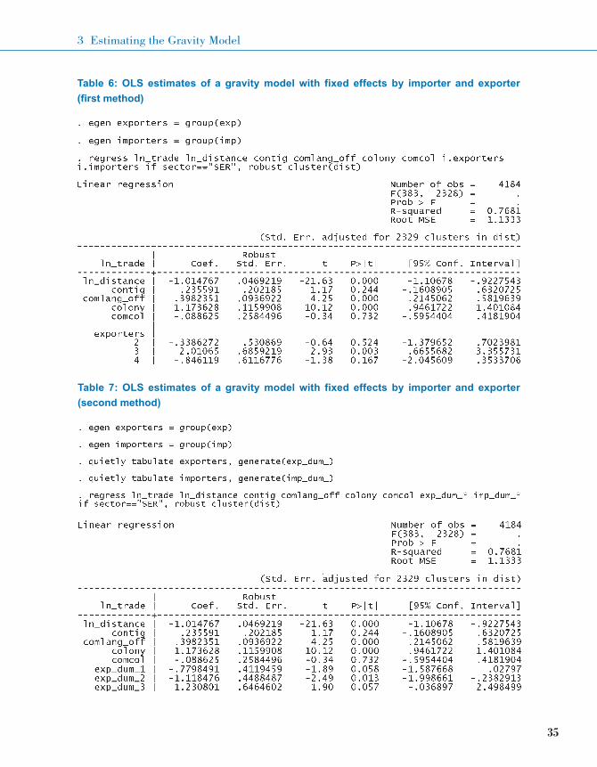
Tables 6 and 7 present results from OLS estimation of a gravity model with exporter and importer

fixed effects using these two approaches. For brevity, Stata’s output is cut off after the first few

exporter fixed effects. As can be seen from the table, the two approaches give exactly identical

results in practice for the variables of interest. The only differences in the two sets of regression

outputs come from the requirement that at least one dummy variable must be dropped in order to

avoid perfect collinearity between the fixed effects and the constant: the first method automatically

chooses a different dummy variable from the second method. There is thus a difference in the

estimated fixed effects between the two methods, but this is of no consequence and simply

represents scaling with respect to an omitted category. The key result is that regardless of which

method is chosen, the estimated coefficients for the variables of interest – which all vary bilaterally

– are identical.

35


Table 6: OLS estimates of a gravity model with fixed effects by importer and exporter

(first method)

Table 7: OLS estimates of a gravity model with fixed effects by importer and exporter

(second method)

36


It is useful to compare results from the fixed effects gravity model with those from the intuitive

model without fixed effects. The first notable feature is that, as expected, the model’s explanatory

power is much greater once the fixed effects are included: it increases from 54 per cent to 77 per

cent. This change is unsurprising given that we have added a large number of additional variables

to the model, but it underlines the important role played by factors such as multilateral resistance

in explaining observed trade outcomes.

The second point to note is that a number of the coefficients are quite different under the two

specifications. The distance elasticity, for example, is very close to -1 under fixed effects, which

is the value typically observed in goods markets. The difference between the estimated elasticity

from the intuitive model and the one from the theoretical model makes clear that the choice of

estimation strategy, and the rationale for it, can make an economically significant difference to

final results.

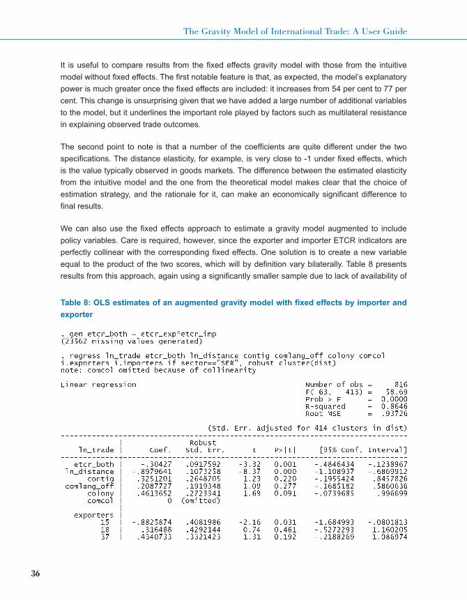
We can also use the fixed effects approach to estimate a gravity model augmented to include

policy variables. Care is required, however, since the exporter and importer ETCR indicators are

perfectly collinear with the corresponding fixed effects. One solution is to create a new variable

equal to the product of the two scores, which will by definition vary bilaterally. Table 8 presents

results from this approach, again using a significantly smaller sample due to lack of availability of

Table 8: OLS estimates of an augmented gravity model with fixed effects by importer and

exporter

37


the ETCR data for non-OECD countries. Again, we find that policy is a significant determinant of

trade flows in services: increasing the product of two countries’ ETCR scores by one point

decreases trade by about 30 per cent, which is a very similar magnitude to the one found using

the intuitive model. The effect is statistically significant at the 1 per cent level.

We have focused thus far on the simple case of aggregate trade, in which multilateral resistance

can be accounted for by including exporter and importer fixed effects in the model. If we add

sectors or time periods to the model, however, the situation becomes more complicated for the

specification of fixed effects, as noted by Baldwin and Taglioni (2007). Consider a sectoral model,

for example:

Collecting terms in this case produces a different arrangement of fixed effects from the aggregate

trade model. Because trade costs potentially vary by sector, the multilateral resistance terms also

vary in that dimension. They can therefore not be adequately captured by importer and exporter

fixed effects. Instead, we need sector, exporter-sector, and importer-sector fixed effects, as

follows:

A second difficulty arises from the fact that the elasticity of substitution also varies across

sectors. Since the reduced form parameters of the trade cost function are joint estimates of the

elasticity of substitution and the elasticity of trade costs with respect to particular factors, it is

important to take account of this variation in a model including multiple sectors. One option would

be to interact the trade cost observables with estimates of the elasticity of substitution from Broda

38


and Weinstein (2006). A simpler alternative would be to interact the trade cost observables with

sector dummies. Although necessary to conform to theory, neither approach is regularly used in

the applied literature.

Fixed effects estimation is a simple and feasible approach in aggregate gravity models. However,

models including a large number of sectors quickly become unmanageable due to the number of

parameters involved. There is no econometric limitation involved – the number of observations is

always far greater than the number of parameters – but gravity models with large numbers of

fixed effects and interaction terms can be slow to estimate, and may even prove impossible to

estimate with some numerical methods such as Poisson and Heckman (see the next section).

A more feasible alternative in such cases is to estimate the model separately for each sector in

the dataset: a separate model for trade in business services versus trade in transport services,

etc. With this approach, all that is needed for each model is a full set of exporter and importer

fixed effects, as in the aggregate trade version of the model. The fact that each sector represents

a separate estimation sample allows for multilateral resistance and the elasticity of substitution to

vary accordingly. Indeed, it can often be useful from a research point of view to estimate separate

sectoral models: knowledge of differences in the sensitivity of trade with respect to policy in

particular sectors can be important in designing reform programmes, for example. This approach

is therefore frequently used in the literature.

3.2.2 Estimation Without Fixed Effects

The fixed effects model provides a convenient way to consistently estimate the theoretical gravity

model: unobservable multilateral resistance is accounted for by dummy variables. The method is

simple to implement and is just an application of standard OLS. It has one important drawback,

however: we need to drop from the model any variables that are collinear with the fixed effects.

This restriction means that it is not possible to estimate a fixed effects model that also includes

data that only vary by exporter (constant across all importers) or by importer (constant across all

exporters). Unfortunately, many policy data – in fact, all policies that are applied on a most-favored

nation basis – fall into this category, which means that the restriction poses a particular challenge

for applied policy researchers.

One way of dealing with this problem is to take variables that vary by exporter or importer and

transform them artificially into a variable that varies bilaterally. This was what we did with the

ETCR scores above: by multiplying them together, the result is a variable that is unique to each

country pair and therefore varies across importers for each exporter and across exporters for each

importer. Such variables can be included in a fixed effects model without difficulty. However, the

price of transforming variables in this way is that the model results become harder to interpret. In

the last table, for example, we cannot distinguish the impact of changes in importer policies from

that of exporter policies, which is potentially an important question. Although the overall policy

message from the last regression was clear, such is not always the case with transformed

39


variables: results can often carry perverse signs or unlikely magnitudes, which mean that

transformation should be used cautiously in policy work.

The panel data econometrics literature provides an alternative to fixed effects estimation that still

accounts for unobserved heterogeneity, but allows the inclusion of variables that would be

collinear with the fixed effects. This alternative is the random effects model. Although it has been

applied in gravity contexts – examples include Egger (2002) and Carrère (2006) – we will not

discuss random effects estimation extensively here. There are two main reasons for not doing

so. First, fixed effects estimation remains largely dominant in the literature because the random

effects model is only consistent under restrictive assumptions as to the pattern of unobserved

heterogeneity in the data. In the context of the theoretical gravity model, the random effects model

requires us to assume that multilateral resistance is normally distributed, yet theory has nothing

to say on that question. The fixed effects specification, by contrast, allows for unconstrained

variation in multilateral resistance. Second, accounting for both inward and outward multilateral

resistance requires specification of a two-dimensional random effects model – random effects by

exporter and by importer – which is rarely treated in the literature. Although such models can be

implemented straightforwardly in Stata using the xtmixed command, they have received scant

consideration either in the econometrics literature or in the applied policy literature. The probable

reason is that fixed effects modeling is generally preferred for gravity work because theoretical

models do not say anything about the statistical distribution of trade costs or multilateral

resistance.

A third, and determinant, consideration is that Baier and Bergstrand (2009) provide an alternative

approach that fully accounts for arbitrary distributions of inward and outward multilateral

resistance but without the inclusion of fixed effects. The Baier and Bergstrand (2009) methodology

therefore makes it possible to consistently estimate a theoretical gravity model that also includes

variables such as policy measures that vary by exporter or by importer, but not bilaterally. Their

approach relies on a first order Taylor series approximation of the two nonlinear multilateral

resistance terms. Concretely, Baier and Bergstrand (2009) show that the following model provides

estimates almost indistinguishable from those obtained using fixed effects, but without the

inclusion of dummy variables:

40


To deal with endogeneity concerns – see below – Baier and Bergstrand (2009) recommend

estimating the model using simple averages rather than GDP-weights. For simplicity, we consider

a Stata application of this approach using distance as the only trade cost variable. The

calculations included here can easily be replicated for other variables, but they are omitted for

brevity in this case. Table 9 presents results from a fixed effects model, and Table 10 presents

results using the Baier and Bergstrand (2009) methodology with simple averages. Clearly, the

two sets of results are very similar: the distance coefficient is only marginally different at the

second decimal place, partly due to differences in the effective samples of the two regressions

because of the absence of GDP data for a small number of countries. This finding shows that the

Baier and Bergstrand (2009) approximation indeed performs well when it comes to capturing the

effects of multilateral resistance in the data without including fixed effects.

Table 9: OLS estimates of a simple gravity model with fixed effects by importer and exporter

Table 10: OLS estimates of a simple gravity model estimated using the Baier and

Bergstrand (2009) methodology

41


3.3 Dealing with Endogeneity

Regardless of whether we are estimating the intuitive gravity model or its theoretical counterpart,

we need to pay particular attention to the problem of endogeneity, particularly when policy

variables are included in the model. The reason is that policies are often determined to some

extent by the level of a country’s integration in international markets: more open economies have

an incentive to implement more liberal policies, for example, which creates a circular causal chain

between policies and trade. From an econometric point of view, endogeneity of an explanatory

variable violates the first OLS assumption by creating a correlation between that variable and the

error term. To see this, we can write down two equations that summarize the problem. The first is

our gravity model:

Table 10: (continued)

The second equation says that trade costs (particularly those driven by policy) are endogenous

to trade flows:

By substitution:

The first OLS assumption will only hold if and are uncorrelated, which is often unlikely in

a practical context. As a result, researchers need to be extremely cautious when interpreting the

results of gravity models with policy variables: the estimated parameters could be severely biased

due to endogeneity, if they are left uncorrected.

Thankfully, basic econometrics provides us with a simple technique to deal with such endogeneity

problems. If we can find an instrumental variable – a piece of data that is correlated with the

42


potentially endogenous variable but not with trade through any other mechanism – then we can

use it to purge the problematic variable of its endogenous variation. Various techniques are

available for instrumental variables estimation, the simplest of which is two stage least squares

(TSLS). As the name suggests, it consists in running OLS twice. The first regression uses the

potentially endogenous variable as the dependent variable, and includes all the exogenous

variables from the model as independent variables, along with at least one additional instrument.

The second regression uses the estimated values of the dependent variable from the first stage

regression in place of the problematic variable in the gravity model itself. We can think of the

estimated values from the first stage as the part of the problematic variable that varies due to

exogenous influences (the instrument and exogenous variables), which solves the endogeneity

problem.3

For the TSLS estimator to work properly and provide results superior to OLS, three conditions

must be satisfied. The first is that there must be at least as many instruments as potentially

endogenous variables, and preferably one extra. Having the same number of instruments as

potentially endogenous variables is a necessary condition for model identification, but including

at least one additional instrument makes it possible to perform an additional diagnostic test that

is an important indicator of instrument validity. The second condition is that the instrumental

variable or variables must be strongly correlated with the potentially endogenous explanatory

variable. To test whether this is in fact the case, we perform an F-test of the null hypothesis that

the coefficients on the instruments are jointly equal to zero in each of the first stage regressions.

First stage F-tests should be systematically reported whenever TSLS is used. The third condition

is that the instruments must be validly excludable from the second stage regression, in the sense

that they do not influence the dependent variable other than through the potentially endogenous

variable. In an over-identified model, we can test whether this condition holds using the Hansen

J-statistic. The null hypothesis for the test is that the residuals from both stages of the regression

are uncorrelated, which is equivalent to assuming that the exclusion condition holds. A high value

of the test statistic (low prob. value) indicates that the instruments may not be validly excludable,

and the TSLS strategy needs to be rethought. Like the first stage F-tests, Hansen’s J should be

routinely reported when it is available.

Although it is possible to run the TSLS estimator manually in Stata, researchers should generally

avoid doing so. One reason is that the standard errors from the second stage regression need

to be corrected in order to avoid downward bias. It is also preferable on a practical level to use

a built in TSLS estimator as it automatically includes the right set of variables in the first stage

regression, i.e. all exogenous variables from the main model plus the instrument.

3 Although correct parameter estimates can be obtained by running OLS twice manually, the estimated standard

errors from the second stage will be biased downwards as they do not correct for the first stage estimation

procedure. Researchers should always use Stata’s built in instrumental variables estimation commands rather

than estimating the models manually.

43


Stata’s built in TSLS estimator is the ivregress command with the tsls option. However, it is

generally preferable to use the user-written ivreg2 command, which contains a host of additional

test statistics and diagnostic information that is important in assessing the performance of the

TSLS estimator. To install ivreg2, simply type findit ivreg2 and follow the prompts. The format for

ivreg2 is similar to regress, but with the addition of some specific information on the endogenous

variables and instruments in parentheses:

ivreg2 dependent_variable exogenous_variables (endogenous_variables = instruments), options

If no additional options are specified, ivreg2 uses TSLS as the estimator. In addition to the

standard robust and cluster options, it is also important to include the first option. This option

presents the first stage regression results, which always need to be reported when TSLS is used.

Another useful option is endog(endogenous variable), which provides a test of the null hypothesis

that the listed variables are in fact exogenous to the model. If the null hypothesis is not rejected

and all other tests for the validity of the TSLS estimator are satisfied, that is an indication that

endogeneity may not be a serious problem in the data. Ivreg2 automatically presents other test

statistics, such as Hansen’s J, if appropriate.

As an example of how the TSLS estimator can be applied to gravity models, we will revert to the

intuitive model augmented to include policy variables, namely the exporter and importer ETCR

scores. We are using the intuitive model for expositional clarity only. In applied work, it would be

important to include fixed effects in addition to the variables discussed here, and TSLS works as

normal in the presence of fixed effects. However, the large number of additional parameters and

the need to transform both the policy variables and instruments to be bilaterally varying makes it

problematic to present such an approach as an example. We therefore use the simpler model for

this purpose.

The first step in applying the TSLS estimator is to identify at least two instruments for the policy

variables (exporter and importer ETCR scores), which are potentially endogenous. Identification

of appropriate instruments is often extremely difficult due to the twin requirements of strength and

excludability discussed above. As an example, we use the absolute value of a country’s latitude

as an instrument for its ETCR score. The rationale is that countries that are further away from

the equator tend to be more developed than those close to the equator, and this is reflected in

a more liberal policy stance. Latitude could also be a proxy for the level of institutional and

governance development, which is also correlated with more liberal policies.

Is latitude likely to be a valid choice of instrument? We will need to examine the first stage

F-tests before deciding whether the correlation with the potentially endogenous variables is strong

enough. We can say with certainty, however, that latitude is genuinely exogenous to the model.

Indeed, researchers often use geographical or historical features as instruments precisely

because they must be exogenous to current variables such as trade flows. The final criterion is

44


excludability. Because the model is just identified, we will be unable to test that condition directly

using Hansen’s J. We therefore need to rely on economic logic to make the argument that latitude

does not affect trade except through the policy measures captured in the ETCR scores. Clearly,

this part of the instrument validity argument is potentially problematic, for at least two reasons.

One is that institutional quality as proxied by latitude might be directly correlated with trade as

a source of trade costs in its own right. A second problem is that distance from the equator is

likely to be correlated with distance from major trading partners, which provides a third possible

way of influencing trade. It is important to stress, therefore, that the instrumental variables strategy

used here is presented as an example only. In published work, it would be necessary to go further

down the path of identifying a more strongly excludable instrument. It would also be highly

preferable to over-identify the model by including at least one extra instrument. Nonetheless, the

basic approach outlined here demonstrates the basic logic of TSLS estimation, and is sufficient

for present purposes.

Table 11 presents estimation results using TSLS. The first part of the Stata output (Table 11a)

shows the first stage regression results for the first potentially endogenous variable, i.e. the

exporter’s ETCR score. We see that the appropriate instrument, namely the exporter’s latitude, is

indeed strongly correlated with the policy variable: the t-test rejects the null hypothesis that the

coefficient is zero at the 1 per cent level, as does the first stage F-test reported at the bottom of

the table. The difference between the two tests is of course that the F-test uses both instruments,

whereas the t-test focuses on one only. Based on these results, we conclude that our instruments

are indeed strongly correlated with the potentially endogenous variables, as required. Moreover,

the direction of the correlation is as expected: countries that are further away from the equator

tend to be more developed, have more liberal trade-related policies, and thus lower ETCR scores

(negative correlation).

Table 11b presents the same output for the second potentially endogenous variable, i.e. the

importer’s ETCR score. Results are nearly identical in every respect. We therefore draw similar

conclusions: latitude is a strong and appropriate instrument for the importing country’s ETCR

score.

Second stage results appear in Table 11c. We find that even after correcting for the potential

endogeneity of the policy variables, they are still negatively and statistically significantly

associated with trade flows. The magnitudes of the coefficients are different from those in the

OLS model, though not by very much. This is a preliminary indication that any bias induced by

endogeneity may not be severe in these data. This impression is reinforced by the endogeneity

test (at the bottom of the table), which does not reject the null hypothesis that the two policy

variables are in fact exogenous to the model. Subject to the validity of the instruments – see

above – we therefore conclude that endogeneity is not a major problem with the policy variables

in this dataset, and that once it is corrected for, the original insight still stands.

45


Table 11a: TSLS estimates of an augmented gravity model

46


Table 11b: TSLS estimates of an augmented gravity model

47


Table 11c: TSLS estimates of an augmented gravity model

Estimating the Gravity Model - unescap.org - 3. Estimating the... · 29 3 Estimating the Gravity...

Documents

Transcript of Estimating the Gravity Model - unescap.org - 3. Estimating the... · 29 3 Estimating the Gravity...