ESTIMATING THE EFFECT OF FUTURE OIL PRICES ON PETROLEUM

ENGINEERING PROJECT INVESTMENT YARDSTICKS

A Thesis

by

ASHISH MENDJOGE

Submitted to the Office of Graduate Studies of

Texas A&M University in partial fulfillment of the requirements for the degree of

MASTER OF SCIENCE

December 2003

Major Subject: Petroleum Engineering

ESTIMATING THE EFFECT OF FUTURE OIL PRICES ON PETROLEUM

ENGINEERING PROJECT INVESTMENT YARDSTICKS

A Thesis

by

ASHISH MENDJOGE

Submitted to Texas A&M University in partial fulfillment of the requirements

for the degree of

MASTER OF SCIENCE Approved as to style and content by: _______________________________

W. J. Lee (Chair of Committee)

_______________________________

Duane A. McVay (Member)

_______________________________ Julian Gaspar

(Member)

_______________________________ Akhil Datta-Gupta

(Member) _______________________________

Hans C. Juvkam-Wold (Head of Department)

December 2003

Major Subject: Petroleum Engineering

iii

ABSTRACT

Estimating the Effect of Future Oil Prices on Petroleum Engineering Project Investment

Yardsticks. (December 2003)

Ashish Mendjoge, B.E., University of Pune

Chair of Advisory Committee: Dr. W. John Lee

This study proposes two methods, (1) a probabilistic method based on historical oil prices

and (2) a method based on Gaussian simulation, to model future prices of oil. With these

methods to model future oil prices, we can calculate the ranges of uncertainty in

traditional probability indicators based on cash flow analysis, such as net present values,

net present value to investment ratio and internal rate of return.

We found that conventional methods used to quantify uncertainty which use high,

low and base prices produce uncertainty ranges far narrower than those observed

historically. These methods fail because they do not capture the “shocks” in oil prices

that arise from geopolitical events or supply-demand imbalances.

Quantifying uncertainty is becoming increasingly important in the petroleum

industry as many current investment opportunities in reservoir development require large

investments, many in harsh exploration environments, with intensive technology

requirements.

Insight into the range of uncertainty, particularly for downside, may influence our

investment decision in these difficult areas.

iv

DEDICATION

To my beloved parents and sister Smita who have always been at my side in any

endeavor, supportive and at times critical.

v

ACKNOWLEDGMENTS

I would like to take this opportunity to express my sincerest appreciation to Dr. John Lee,

my advisor, for his help in constructing and completing this thesis. It was a really

wonderful opportunity to work with him. His guidance through the discussions and

suggestions activated my thought processes and generated a great deal of interest in the

thesis work, giving me self-belief and a feeling of responsibility.

I wish to take the opportunity to thank and acknowledge Dr. Duane McVay, for

his helpful comments, guidance and friendliness during the meetings.

I thank Dr. Julian Gaspar and Dr. Akhil Datta-Gupta, for agreeing to be on my

supervisory committee and reviewing the entire thesis work. At this opportune moment, I

would like to convey my appreciation to Dr. Tom Blasingame for giving me the chance

to join the Texas A&M Petroleum Engineering Department family and for selecting me

to receive the Texaco Fellowship.

I would also like to thank Mukesh Masand for our memorable friendship and his

support and suggestions in brainstorming sessions. The facilities and resources provided

by the Harold Vance Department of Petroleum Engineering, Texas A&M University, are

gratefully acknowledged.

I thank Texas A&M University for educating me in various ways, and for

providing me with the very best education. I would like to take the opportunity to thank

the faculty and staff for helping me prepare for a life after graduation.

I am going to remember these years of hard work with great pleasure. To all of

you, I appreciate what you have done to help me in my scholastic and professional

growth.

vi

TABLE OF CONTENTS

Page

ABSTRACT ……………………………………………………………................... iii

DEDICATION……………………………………………………………............... iv

ACKNOWLEDGMENTS…………………………………………………………. v

TABLE OF CONTENTS…………………………………………………………... vi

LIST OF FIGURES………………………………………………………………… vii

LIST OF TABLES…………………………………………………………………. x

CHAPTER

I INTRODUCTION……………………………………………………... 1

II REVIEW OF LITERATURE ON UNCERTAINTY………………….

Introduction……………………………………………….. Sources of uncertainty…………………………………….. Types of uncertainties……………………………………..

4

4 5 5

III METHODOLOGY ...…………………………………………………..

Economic indicators ……………………………………… Conventional analysis ……………………………………. Application of historical method to typical cash flow stream Application of Gaussian simulation model to typical cash

flow streams ………………………………………………... Application to field case …………………………………….

9

12 15 16

19 21

IV RESULTS………………………………………………………………

Results for typical cash flow streams………………………..

25

V CONCLUSIONS AND FUTURE WORK ………….………………... 39

REFERENCES……………………………………………………………………... 41

APPENDIX A………………………………………………………………………. 44

APPENDIX B………………………………………………………………………. 54

VITA………………………………………………………………………………... 55

vii

LIST OF FIGURES

FIGURE Page

3.1 Historical West Texas Intermediate (WTI) crude price profile……...... 10

3.2 Historical trend of consumer price index……………………………… 11

3.3 WTI crude price production cost correlation ………….……………… 11

3.4 WTI crude price drilling cost correlation ……………………….......... 12

3.5 Representative petroleum project annual cash flow profile…………… 14

3.6 Price scenarios for high most-likely, low and base cases used in

conventional analysis………………………………………………...... 16

3.7 Historical price path and derived inflation indices for 1975 and 1983 . 17

3.8 Comparison of historical and uninflated price path for 1975 and 1983 . 18

3.9 Comparison of actual and average price scenarios for 1975 and 1983 . 18

3.10 Comparison of historical and average price scenarios for 1975 and

1983 …………………………………………………………………… 19

3.11 Comparison of actual and uninflated crude prices .…………………… 20

3.12 Uninflated and inflated scenarios built from G.S. method ……………. 21

3.13 Normalized oil price scenarios from G. S. method ...………………..... 21

3.14 Oil production scenarios with and without injection …………………. 24

4.1 Cash flow ranges obtained for decreasing cash flow case by

conventional methods………………………………………………….. 27

4.2 Cash flow ranges obtained for decreasing cash flow case by historical

methods………………………………………………………………... 27

4.3 Cash flow ranges obtained for decreasing cash flow case by Gaussian

Simulation methods ………………………………………………….... 28

4.4 Cash flow ranges obtained for increasing cash flow case by

conventional methods………………………………………………….. 28

4.5 Cash flow ranges obtained for increasing cash flow case by historical

methods………………………………………………………………... 29

viii

FIGURE Page

4.6 Cash flow ranges obtained for increasing cash flow case by Gaussian

simulation methods ……………………................................................ 29

4.7 Cash flow ranges obtained for constant cash flow case by

conventional methods………………………………………………….. 30

4.8 Cash flow ranges obtained for constant cash flow case by historical

method…………………………………………………………………. 30

4.9 Cash flow ranges obtained for constant cash flow case by Gaussian

simulation method …………………………………………………….. 31

4.10 Uncertainty ranges for decreasing cash flow case with NPV/I -10%

yardstick……………………………………………………………….. 33

4.11 Uncertainty ranges for decreasing cash flow case with NPV -10%

yardstick……………………………………………………………….. 33

4.12 Uncertainty ranges for decreasing cash flow case with internal rate of

return yardstick………………………………………………………… 34

4.13 Uncertainty ranges for increasing cash flow case with NPV/I -10%

yardstick……………………………………………………………….. 34

4.14 Uncertainty ranges for increasing cash flow case with NPV -10%

yardstick……………………………………………………………….. 35

4.15 Uncertainty ranges for increasing cash flow case with internal rate of

return yardstick………………………………………………………… 35

4.16 Uncertainty ranges for constant cash flow case with NPV/I -10%

yardstick……………………………………………………………….. 36

4.17 Uncertainty ranges for constant cash flow case with NPV -10%

yardstick……………………………………………………………….. 36

4.18 Uncertainty ranges for constant cash flow case with internal rate of

return yardstick ………...……………………………………………… 37

4.19 C.D.F. of incremental recovery case showing range of net present

value………………………………………………………………….. 38

4.20 Uncertainty range comparison for incremental recovery case……….. 38

ix

LIST OF TABLES

TABLE Page

3.1 Representative projects with the economic indicators………………… 15

3.2 Capital costs summary for incremental recovery project……………… 22

3.3 Well operating costs summary for incremental recovery project…….. 23

3.4 Gas injection operating summary for incremental recovery project….. 23

3.5 Drilling cost and price of crude for incremental recovery project…….. 23

4.1 Ranges in values of investment evaluation indicators, decreasing cash

flow case ………………………………………………………………. 25

4.2 Ranges in values of investment evaluation indicators, increasing cash

flow case ………………………………………………………………. 25

4.3 Ranges in values of investment evaluation indicators, constant cash

flow case ………………………………………………………………. 26

4.4 Ranges of Gaussian simulation as percentage of historical method…... 31

4.5 Uncertainty range for incremental recovery project ………………….. 38

1

CHAPTER I

INTRODUCTION

Exploration and development of oil and gas resources is a fast paced, continually

evolving industry that experiences drastic changes due to changes in market conditions.

Predicting growth and maintaining competitive advantage by managing cash flows,

operating income and resource requirement in a volatile market is a challenge for

operating companies. This is due to the inherent risk and uncertainty involved.

Now as we are progressing toward exploration of oil in deeper and harsh

environments with harder to find traps involving much greater levels of uncertainty,

estimation and quantification of uncertainty is gaining importance.

Begg and Bratvold1 report that, over the past ten years, oil and gas companies

have significantly under performed in the stock market compared to the Dow Jones

Industrial Average Index. This is true for both majors and independents. An

understanding of the causes of the industry’s poor performance is a prerequisite to

improving it.

Brashear and Becker2 have given a similar review; projects undertaken in last two

decades had an average return of 7%. This is in spite of improvement of 90% in

exploration success rate and of as much as 30% in development success rate due to 3-D

seismic technology. These projects were selected on the basis that they surpassed the

criteria of internal minimum rate of return of 15% or more.

There are myriad of factors, but dominant among them are the impacts on the

value that derive from the existence of uncertainty. If there were no uncertainty then,

apart from deliberate misrepresentation, returns would always have been as predicted.

The failure of many investments to deliver predicted returns implies over or under

estimation of risk or loss.

McMichael3 stated that oil and gas prices are essential elements in economic and

reserves calculation and that the prices have at least as large an impact on project

economic performance as the uncertainties in the reservoir and technical data. Forecasts

of oil and gas prices are pivotal points in development decisions due to their impact on

______________________________

This thesis follows the style and format of SPE Reservoir Evaluation.

2

project economic viability and reserves.

Kokolis and Litvak4 et al. pointed out that the uncertainty is greatest in petroleum

exploration and production (E&P) projects at the early or inception stages of the venture.

Generally it is during that time frame when bidding decisions have to be made in spite of

the available minimum information. To analyze a project effectively, we should come up

with a range in investment yardsticks that will have rational upside and down side values

scenarios to constrain bid levels to assure at least marginal success in low-end outcomes.

Conventional methods of characterizing uncertainty include methods where

forecasts are represented by monotonic increase of inflation indices and corresponding

changes on dependent parameters such as crude price and expenses

Underlying correlations existing in the parameters are often overlooked in

conventional analysis. Brashear and Becker5et al. state that people generally estimate the

below ground uncertainties in reservoir and geologic parameters but they fell to recognize

above ground uncertainties that include future price and costs; changes in demand and

transportation storage system, changes in technology for exploration, production and

transportation. The formulation and incorporation of these parameters in the analysis

gives better estimation of uncertainty associated with it. Correlations have been

developed based on historical oil price, production cost and drilling expenditures will

make projections more realistic.

Discounted cash flow (DCF) methods described by Downs and Goodman6 as

techniques that calculate value of future expected cash receipts and expenditures using

net present value as a factor at a common or starting date are commonly used as part of

conventional investment analysis. Surveys made by Dougherty and Sarkar7 among oil

and gas companies, investment advisors and bank engineers have demonstrated that

almost 97 percent of respondents use DCF as their primary investment evaluation

method.

The focus of this research is on better quantifying the economic uncertainty in

petroleum projects caused by uncertainty in future oil prices.

3

The two broad objectives of this study are:

• To quantify the uncertainty in investment evaluation indicators caused by

uncertainty in the future price of oil.

• To develop a model to predict future prices of oil including uncertainty ranges,

based on past prices of oil.

These objectives lead to five deliverables listed below:

1. A model for predicting the inflation adjusted future price of oil based on methods

used in geostatistics.

2. Comparison of common investment evaluation yardsticks (NPV, NPV/I, IRR) for

a typical oil field project determined using

o Conventional analysis (including most likely, high and low price cases)

o Actual price trends and operating expenses

3. Comparison of common investment evaluation yardsticks for the same typical oil

field project determined using

o Conventional analysis

o Oil Price forecasting model

We will generate sufficient number of cases with the statistically valid sample.

4. Comparison of common investment yardsticks for a representative variety of

cash flow profiles reported in literature using

o Conventional analysis

o Actual price trends and operating expenses

5. Comparison of common investment evaluation yardsticks for a representative

variety of cash flow profiles reported in the literature using

o Conventional analysis

o Oil price forecasting model

4

CHAPTER II

REVIEW OF LITERATURE ON UNCERTAINTY

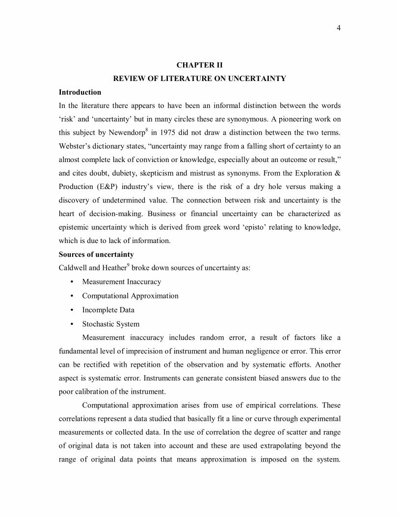
Introduction

In the literature there appears to have been an informal distinction between the words

‘risk’ and ‘uncertainty’ but in many circles these are synonymous. A pioneering work on

this subject by Newendorp8 in 1975 did not draw a distinction between the two terms.

Webster’s dictionary states, “uncertainty may range from a falling short of certainty to an

almost complete lack of conviction or knowledge, especially about an outcome or result,”

and cites doubt, dubiety, skepticism and mistrust as synonyms. From the Exploration &

Production (E&P) industry’s view, there is the risk of a dry hole versus making a

discovery of undetermined value. The connection between risk and uncertainty is the

heart of decision-making. Business or financial uncertainty can be characterized as

epistemic uncertainty which is derived from greek word ‘episto’ relating to knowledge,

which is due to lack of information.

Sources of uncertainty

Caldwell and Heather9 broke down sources of uncertainty as:

• Measurement Inaccuracy

• Computational Approximation

• Incomplete Data

• Stochastic System

Measurement inaccuracy includes random error, a result of factors like a

fundamental level of imprecision of instrument and human negligence or error. This error

can be rectified with repetition of the observation and by systematic efforts. Another

aspect is systematic error. Instruments can generate consistent biased answers due to the

poor calibration of the instrument.

Computational approximation arises from use of empirical correlations. These

correlations represent a data studied that basically fit a line or curve through experimental

measurements or collected data. In the use of correlation the degree of scatter and range

of original data is not taken into account and these are used extrapolating beyond the

range of original data points that means approximation is imposed on the system.

5

Caldwell and Heather9 quote the example of net pay determination in reserves calculation

for the source of computer approximation.

The cost factor of data collection gives rise to the third source of uncertainty

which is incomplete data. The problem is generally tackled by making suitable

assumptions. These assumptions vary according to the experience of the person, and his

competence to acknowledge the uncertainty, which gives rise to the bias. Purvis10 lists

ten different types of bias commonly observed in making decisions. The most important

one is the overconfidence or pride bias. People get anchored to their first assumption of

an uncertain quantity and do not move away from it11. Capen12 exposed this pride bias

with a ten item quiz that was based on general knowledge and empirical experiments of

bean counting that asked engineers to put down ranges bracketing the answers. He

demonstrated engineers are not accustomed to predict the ranges of uncertainty; what

they believe to be ninety percent confidence interval frequently turns out to be forty or

fifty percent of the actual interval. However with repeated calibration people can be

trained to improve their skills in estimating uncertainty. Capen also noted that when, the

knowledge of the subject is little, smaller ranges are assigned to uncertainty.

Stochastic parameters are factors which are outside the realm of engineering

estimates but are continually at play and affect final answers significantly. Caldwell13

recognized the stochastic nature of the crude oil prices. His observation was that 94

percent of the time crude prices behave as if they were normally distributed. These

stochastic parameters have more significant impact on projects than the ultimate

recovery. The cyclical nature of oil prices makes investment patterns in exploration and

production industry (E&P) equally cyclical14. Oil price volatility correlates with all

facets of the business, starting with exploration drilling activity, research and

development, employment and labor trends leading to mergers and mega mergers in the

industry.

Types of uncertainties

Garb15 identified three kinds of the uncertainty in E&P projects: (1) technical, (2) political and (3) economical.

Technical uncertainty relates to whether or not the hydrocarbon volume estimated

by geologists and engineers exists in the ground and whether or not the reserves and

6

recovery rates will be as projected by the engineers. Demirmen16 further described

technical uncertainty as a function of how long the property has produced and the

maturity and quality of the database from which the reserves determinations were

developed and showed technical uncertainty as various forms of reservoir uncertainty.

Reservoir uncertainty is the function of three parameters: (1) hydrocarbon in place

volume (e.g. structure), (2) recovery factor or productivity (e.g. aquifer strength and

reservoir oil saturation) and (3) fluid properties of reservoir fluids, to gas composition

and crude viscosity. There is also technical uncertainty in operations such as drilling,

number of platforms and their construction time and cost and facility development that

relates to gathering and export lines size and cost.

Political uncertainty could materially influence the expected value of a producer’s

property. It includes not only local and national taxes but environmental regulations,

operational restrictions and global concerns including international instability.

Economical uncertainty deals with capital investment, operating expenses, prices,

inflation and exchange rates. The investments in E&P projects are frequently medium to

long term with high degree of irreversibility. Oil price uncertainty is the chief variable

here. The cost of incorrectly anticipating long-term oil price behavior has proved

staggering17. Sadorsky18 noted that, “Changes in oil price have an impact on economic

activity but changes in economic activity have very little impact on oil prices.” He stated

that oil price volatility shocks have asymmetric effects on the economy and provided

evidence of the importance of oil price movements when explaining movements in stock

returns. The real challenge is not try to make forecasts more accurate through technical

advances; rather, it is to shift focus to developing better ways to use forecast and to

develop planning mechanisms that help to anticipate and prepare for contingent

developments.

To manage this price risk effectively and to increase their profitability, E&P

companies make use of derivative instruments such as forwards, futures and options.

Companies can lock in profits by hedging a portion of their production and through paper

trading in adverse price movements. The hedging strategies do not create value but their

wise use reduces the variance of earnings or the variance of project profitability19.

7

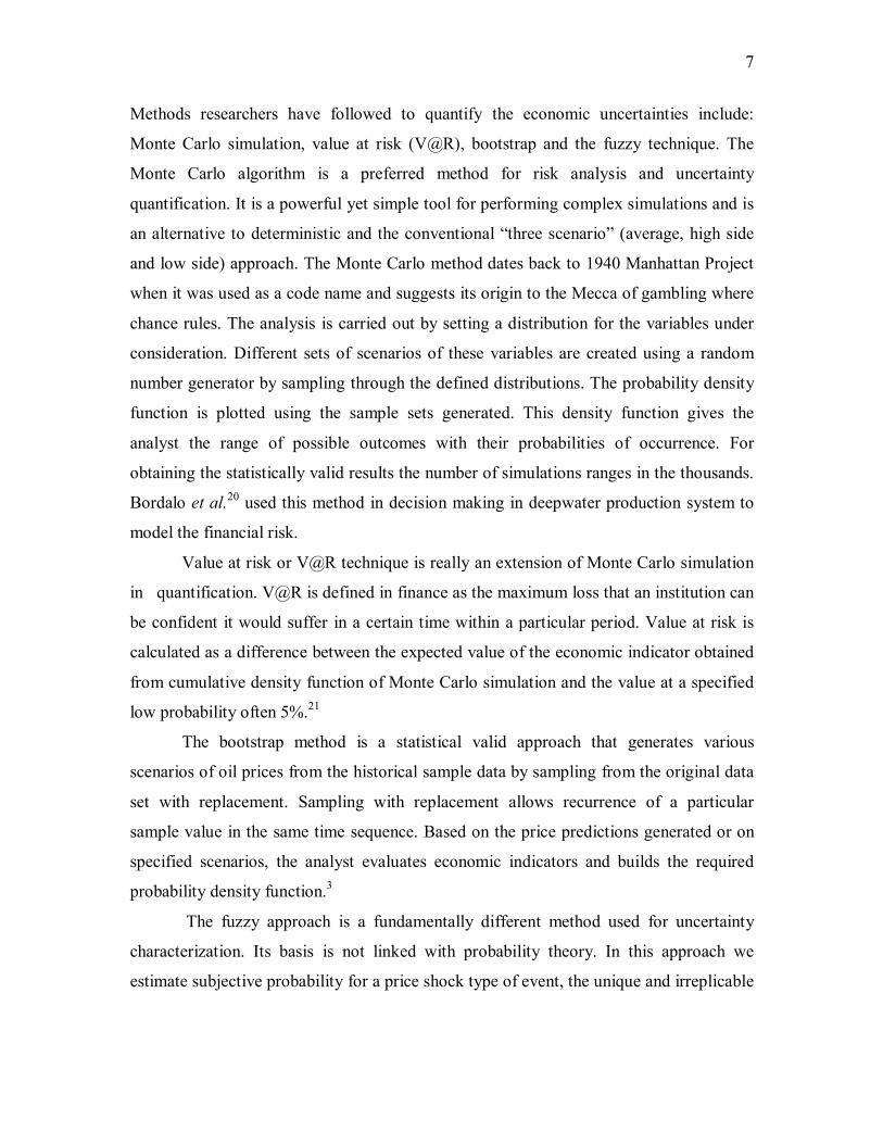
Methods researchers have followed to quantify the economic uncertainties include:

Monte Carlo simulation, value at risk (V@R), bootstrap and the fuzzy technique. The

Monte Carlo algorithm is a preferred method for risk analysis and uncertainty

quantification. It is a powerful yet simple tool for performing complex simulations and is

an alternative to deterministic and the conventional “three scenario” (average, high side

and low side) approach. The Monte Carlo method dates back to 1940 Manhattan Project

when it was used as a code name and suggests its origin to the Mecca of gambling where

chance rules. The analysis is carried out by setting a distribution for the variables under

consideration. Different sets of scenarios of these variables are created using a random

number generator by sampling through the defined distributions. The probability density

function is plotted using the sample sets generated. This density function gives the

analyst the range of possible outcomes with their probabilities of occurrence. For

obtaining the statistically valid results the number of simulations ranges in the thousands.

Bordalo et al.20 used this method in decision making in deepwater production system to

model the financial risk.

Value at risk or V@R technique is really an extension of Monte Carlo simulation

in quantification. V@R is defined in finance as the maximum loss that an institution can

be confident it would suffer in a certain time within a particular period. Value at risk is

calculated as a difference between the expected value of the economic indicator obtained

from cumulative density function of Monte Carlo simulation and the value at a specified

low probability often 5%.21

The bootstrap method is a statistical valid approach that generates various

scenarios of oil prices from the historical sample data by sampling from the original data

set with replacement. Sampling with replacement allows recurrence of a particular

sample value in the same time sequence. Based on the price predictions generated or on

specified scenarios, the analyst evaluates economic indicators and builds the required

probability density function.3

The fuzzy approach is a fundamentally different method used for uncertainty

characterization. Its basis is not linked with probability theory. In this approach we

estimate subjective probability for a price shock type of event, the unique and irreplicable

8

nature of which makes determining the probability difficult. Researchers of this discipline

include the theory of possibility as an extension of fuzzy sets.22

9

CHAPTER III

METHODOLOGY

We developed two methods in our research to predict the ranges of uncertainty in oil

prices. Both methods are based on historical price data.

The price of oil is affected by three major factors demand-supply, inflation and

geo-political events. The historical method removes inflation from oil prices and thus

makes it a function of the two remaining factors. Major geo-political events are a strong

driving factor in the volatility of inflation adjusted crude prices. When we include this

event-generated volatility structure in a model that predicts for the future, we assume that

the volatility will be repeated in the future.

Scenario generation depends on the year a project is implemented and on project

duration. The scenarios are then built as discussed at length in the following pages. The

range of values the method predicts for oil prices reflect the actual uncertainty observed

in the historical price pattern and the range is directly correlated with the volatility

observed in the past.

The second method is based on geostatistical simulation technique of Sequential

Gaussian Modeling (SGM). The SGM generates the simulation of future oil prices using

a variogram. The algorithm draws a random path through unconditioned cells and, for

each cell along the random path; it locates a prespecified number of surrounding

conditioned data. This local neighborhood is selected conforming to the range of

variogram so the same correlation exists in the predicted price as observed in history.

Then, performing ordinary krigging it obtains the mean of Gaussian distribution and the

variance which are sufficient to determine the Gaussian function. The procedure is

repeated to obtain the desired number of simulations. The use of a price histogram and

variogram generates the range of simulated values with same frequency and correlation

and so these eqi-probable scenarios represent the historical price pattern and provide a

good measure of uncertainty.23-24

The first step in this project was of data gathering. We selected West Texas

Intermediate (WTI) spot oil price data starting in January 1974 as our price basis. Though

abundant data is available for crude oil prices at earlier dates we chose to use data from

1974 onward because prior to 1974 posted prices were common in the oil industry.

10

Posted oil prices remained stable over long periods while daily prices fluctuated; thus

posted price did not reflect the true volatility in crude oil prices. The name posted oil

price was derived from a sheet that was posted in a producing field.

The WTI price data were collected from Energy Information Administration

(EIA) website25. EIA provides daily price data; it was converted to monthly price for use

in this study.

Fig.3.1 shows oil price data from 1974 to 2002 (348 months). Fig. 3.2 shows the

historical trend of the consumer price index normalized with respect to 1983. The source

for consumer price index (C.P.I) data is U.S. Department of Labor Bureau of Labor

Statistics26. The data is non-seasonally adjusted data for all urban consumers. The data

frequency is monthly.

To account for production and drilling expenses in future projects; we correlated

historical expenses data with oil price. Figs. 3.3 and 3.4 are graphs of the production and

drilling costs correlations with oil price. The historical oilfield drilling and production

data was taken from EIA website and the Energy Statistics Sourcebook27-28. This data is

available on yearly basis for 15-year period from 1986 to 2001. A linear trend line with a

regression coefficient of 0.30 was fitted for the production data. The drilling expense has

a regression coefficient of 0.73 with a power-type trend line.

Fig. 3.1- Historical West Texas Intermediate (WTI) crude price profile.

1.00

10.00

100.00

Jan-73 Nov-76 Sep-80 Jul-84 May-88 Mar-92 Jan-96 Nov-99 Sep-03

Time (month)

Oil

Pric

e ($

/Bbl

11

10.0

100.0

1000.0

Apr-72 May-76 Jun-80 Aug-84 Sep-88 Oct-92 Dec-96 Jan-01

Time (month)

CPI

CPI

Fig 3.2- Historical trend of consumer price index.

Fig. 3.3- WTI crude price production cost correlation.

14,000

19,000

24,000

29,000

34,000

39,000

44,000

49,000

54,000

10.00 20.00 30.00 40.00 50.00 60.00 70.00 80.00 90.00oil price($/bbl)

Prod

cos

t ($/

# W

ell

cost-prod

Linear (cost-prod)

y = 427.81x + 11830R2 = 0.3096

12

Fig. 3.4- WTI crude price drilling cost correlation.

Economic indicators

For the economic evaluation of exploration and production projects two types of

investment yardsticks are used. These two types of economic indicators or yardsticks are

differentiated on the basis of time value of money concept. The basic principle of time

value of money is that a dollar received today is worth more than a dollar to be received

sometime in the future.29

Our economic indicator account for the time value of money by ‘discounting’

future net revenues by a prescribed interest or hurdle rate. Discounted future revenue is

the present value, Vp, which for a single cash flow is written as

Vp = Fp (1+i)-n …………………………………………………….(1)

and for a cash flow stream is written as

( ) ( ) j

j

n

jPp iFV −

=

+=∑ 11

………………………………………………….(2)

where Fp is the period cash flow “future” value, i is the interest rate and n (or j) is the

number of periods in the future.

50000

200000

350000

500000

650000

800000

950000

1100000

0.00 10.00 20.00 30.00 40.00 50.00 60.00 70.00 80.00 90.00Oil Price ($/Bbl)

Dril

ling

Cos

t ($/

#w

ell

drilling correlation

Pow er (drilling correlation)

y = 54507.91((X) (̂0.6519))R2 = 0.7332256

13

Discounted net revenue or net present value (NPV) is calculated by replacing the

future value in Eqs. 1 and 2 with the net future value. Present value and net present value

calculations for investment streams contain both cash inflow and outflow; thus both can

be positive or negative. A positive NPV at or above company’s hurdle rate is the chief

criteria in project selection because it is simply the capital created above the cost of

capital to a company.

NPV/I is the ratio of a project’s NPV to the present value of the total investment

required for the project. It can be written as

pi

npDi V

VR = …………………………………………………..(3)

This indicator may also be viewed as the amount of after tax NPV generated for

dollar of discounted investment. NPV/I is derived from NPV and thus bears its all

advantages. It is a preferred tool in the ranking of projects when capital requirements

exceed the total available capital. Another useful feature of NPV/I is that it is

independent of the choice of data to which present values are referred (sometimes called

“time zero”). This feature is useful when we compare projects with different starting

dates.

Internal Rate of Return (IRR) is the rate that makes the NPV of a project equal

zero. This investment criterion is popular because it is independent of discount and hurdle

rate. However it is not reliable for ranking projects.

We first examined the uncertainty in typical oilfield project cash flow stream

using historical price data and developed our correlations. Capen30 et al. presented the

“base case” array of project cash flow streams we examined. We modified the annual

cash flow streams as described below and calculated net present value (NPV), net present

value to investment ratio (NPV/I) and internal rate of return (IRR) for the base case and

for each of the modified cases.

Table 3.1 presents the streams of annual cash flow for the base case (constant oil

prices) of our three representative projects, along with economic indicators. Fig. 3.5

illustrates the cash flows over the 10-year project lives.

14

Fig. 3.5- Representative petroleum project annual cash flow profile.

To study the economic uncertainty we then modified the cash flow streams to

reflect variable oil prices. First we converted annual cash flows to monthly cash flows

and generated monthly oil production schedules. To preserve the original economic

indicators (NPV, NPV/I etc.) we generated oil production schedules using an oil price of

20.5 $/STB (any scenario e.g. January 1975 price profile) and set revenues from this

production stream equal to 110% of the cash flows proposed by Capen30, et al. Said

another way operating expenses were 10% of the total revenues. In these cash flow

streams; all investments such as drilling and facilities occurred in year zero.

-12000

-10000

-8000

-6000

-4000

-2000

0

2000

4000

6000

8000

0 1 2 3 4 5 6 7 8 9 10 11

Year

Cash

Flo

w ($

)

decreasing increasing constant

15

TABLE 3.1 - Representative Projects with the Economic Indicators

Annual Cash Flow Year Project-

Decreasing Project-

Increasing Project- Constant

0 -10,000 -5,000 -10,000 1 6,000 0 2,100 2 4,000 0 2,100 3 3,000 250 2,100 4 2,000 250 2,100 5 500 500 2,100

6 200 1,500 2,100 7 100 2,500 2,100 8 100 3,500 2,100 9 50 3,500 2,100 10 50 2,500 2,100

Economic indicators value for most likely case

IRR (%) 24.8 14.6 16.4 NPV @ 5% ($) 4,322 4,869 6,215 NPV @ 10% ($) 2,942 1,879 2,903 NPV @ 15% ($) 1,789 (98) 539

NPV/I @ 5% 0.43 0.97 0.62 NPV/I @ 10% 0.29 0.38 0.29 NPV/I @ 15% 0.18 (0.02) 0.05

Conventional analysis

Following simple methodology similar to that used in practice by some analysts; we then

analyzed each of these projects with high, low and most-likely oil price forecast.

For the most likely case, we assumed that the price of oil would escalate at an

annual inflation rate of 5.2% (compounded monthly). This was the average rate of

inflation in CPI over the 348-month period we investigated. The high price case assumed

oil price escalated at an annual rate of 10.6% (compounded monthly). To calculate the

escalation in price and in turn to generate the cash flow stream. For the low price case we

16

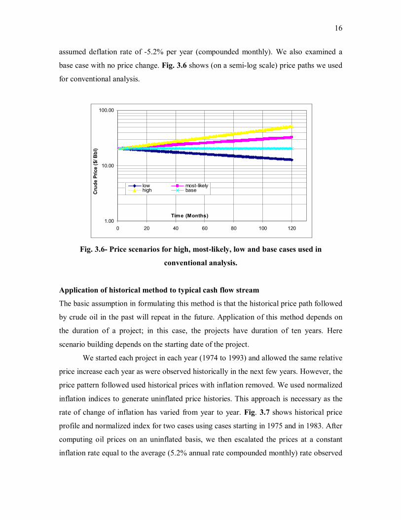
assumed deflation rate of -5.2% per year (compounded monthly). We also examined a

base case with no price change. Fig. 3.6 shows (on a semi-log scale) price paths we used

for conventional analysis.

Fig. 3.6- Price scenarios for high, most-likely, low and base cases used in

conventional analysis.

Application of historical method to typical cash flow stream

The basic assumption in formulating this method is that the historical price path followed

by crude oil in the past will repeat in the future. Application of this method depends on

the duration of a project; in this case, the projects have duration of ten years. Here

scenario building depends on the starting date of the project.

We started each project in each year (1974 to 1993) and allowed the same relative

price increase each year as were observed historically in the next few years. However, the

price pattern followed used historical prices with inflation removed. We used normalized

inflation indices to generate uninflated price histories. This approach is necessary as the

rate of change of inflation has varied from year to year. Fig. 3.7 shows historical price

profile and normalized index for two cases using cases starting in 1975 and in 1983. After

computing oil prices on an uninflated basis, we then escalated the prices at a constant

inflation rate equal to the average (5.2% annual rate compounded monthly) rate observed

1.00

10.00

100.00

0 20 40 60 80 100 120

Time (Months)

Cru

de P

rice

($/ B

bl)

low most-likelyhigh base

17

over the 348-month historical period we examined. We then calculated normalized oil

price indices for each month during the historical period.

To compare the various scenarios on same basis, the oil price in the first month

was fixed at 20.5 $/STB for all starting dates. We then multiplied the starting price by the

indexed values appropriate for the starting year we examined and generated monthly oil

prices. Fig. 3.8 shows the uninflated price scenarios generated using this procedure and

compares then with the actual prices for scenarios with starting dates of 1975 and 1983.

Depending on project conditions we included drilling and production correlations with oil

price in our project cash flow streams. The investments for all projects took place in year

zero. The production schedule for project (flat, decrease, increase) was fixed and when

oil price forecasts and operating costs were applied, we generated cash flow streams for

each project starting in year 1974 to 1993. For each of the generated scenario economic

yardsticks are calculated and are evaluated against the base case.

From the economic indicators that we calculated, we generated probability

density functions (P.D.F.) and cumulative density functions (C.D.F.) for each project and

evaluated the variation in indicator.

Fig. 3.7- Historical price path and derived inflation indices for 1975 and 1983.

1.0

10.0

100.0

0 20 40 60 80 100 120 140

Time (month)

Oil

Pric

e ($

/Bbl

)

0.950

1.150

1.350

1.550

1.750

1.950

2.150

Infla

tion

Inde

x

1975act 1983act1975indx 1983indx

18

Fig. 3.8- Comparison of historical and uninflated price path for 1975 and 1983.

Fig. 3.9- Comparison of actual and average price scenarios for 1975 and 1983.

1.0

10.0

100.0

0 20 40 60 80 100 120

Time (month)

Oil

Pric

e ($

/Bbl

)

1975act 1983act75avg 83avg

1.0

10.0

100.0

0 20 40 60 80 100 120 140Time (months)

Oil

Pric

e ($

/Bbl

)

1975unf l 1983unfl1975act 1983act

19

Fig. 3.10- Comparison of historical and average price scenarios for 1975 and 1983.

Application of Gaussian simulation model to typical cash flow streams

We also developed a model to predict future prices of WTI crude oil using Gaussian

simulation and used those predictions of oil prices to quantify the uncertainty in the

representative oilfield projects (Capen’s flat, increasing and decreasing cash flow

streams).

The basic requirement was to generate equi-probabable scenarios of future oil

prices. To generate these predictions we used the Sequential Gaussian Modeling (SGM)

technique. Two available geostatistical software packages; GEOEAS and GSLIB, were

used to carry out SGM technique.

SGM requires normally distributed input data. The input data in this case were

historical oil prices and its semi variogram from which we obtained correlation matrix.

We actually used the inflation adjusted historical oil price data illustrated in Fig. 3.11 and

tabulated in appendix. The adjusted and uninflated oil prices were generated relative to a

inflation index of 1.0 in 1974. The figure shows that the distribution of the prices is multi

modal or with more than one peak as the SGM demands input data to be normal a

transformation technique had to be used. Using the normal score transform technique

from the GEOEAS package, we converted the multi-modal historical oil price data to uni-

modal or normally distributed data. The normal score technique accomplishes this by

ranking the data and assigning a normal score using the identical quantile of a standard

1.0

10.0

100.0

0 20 40 60 80 100 120Month

His

toric

al M

etho

d ($

/ Bb

1975 198375avg 83avg

20

normal distribution. The semi variogram for this normally distributed data was modeled

using a spherical model and setting the seal value equal to one. The range obtained by

modeling the semi variogram was fed to the simulator with the histogram of the

uninflated oil price data to generate the prediction scenarios. A total of fifty uninflated oil

price prediction scenarios were generated to analyze the uncertainty range of the typical

oil field project. The average inflation index was modeled as function of time in months

with a starting value of month set to 348 (the end of historical data). Fig. 3.12 shows

three representative prediction scenarios of the uninflated crude oil price and the same

scenarios with inflation added at an annual rate of 5.2 per cent (compounded monthly).

We then adjusted these inflated price predictions to a starting value of 20.5$/STB. We

then used these results of price forecasts to generate cash-flows for typical petroleum

projects and thereby calculated the range of uncertainty based on the reference starting

price 20.5$/STB.

Fig. 3.13 shows the price ranges obtained by this method.

Fig. 3.11- Comparison of actual and uninflated crude prices.

1

10

100

May-73 Aug-76 Dec-79 Mar-83 Jul-86 Oct-89 Jan-93 May-96 Aug-99 Dec-02

month

Oil

pric

e ($

/ bb

l)

actual price

uninflated price

21

Fig 3.12- Uninflated and inflated scenarios built from G.S. method.

Fig 3.13- Normalized oil price scenarios from G.S. method.

Application to field case

The third part of this research was to apply the historical method developed earlier to a

real field case of incremental oil recovery in a six year duration project. The objective

was to determine the feasibility of undertaking incremental recovery by gas and water

injection. To do this we selected net present value as the optimization variable. We

10

100

0 20 40 60 80 100 120Time (month)

Oil

Pric

e ($

/Bbl

)

Sim-1 Sim-2Sim-3

1

10

100

0 20 40 60 80 100 120Time (month)

Infla

ted

Oil

Pric

e ($

/Bb

1-unfl 2-unfl 3-unfl1-infl 2-infl 3-infl

22

developed an economics model that would allow us to estimate the net present value

using the input and output data from obtained history match run. Major costs, prices and

assumptions of this model are presented in Table 3.2 to 3.5. Production forecasts with

and without gas injection in the field were available. Monthly oil, gas and water

production data were available for each well. A gas injection well was proposed to be

drilled in the 6th month from start date. The produced gas had to be compressed and the

compression cost per MMSCF was available.

For the injection case, installation of the gas compressor and water injection

facility costs were added. The produced gas was reinjected along with makeup gas and

the compression cost for this operation was calculated on monthly basis. The operating

costs for production and gas, water injection with the cost of operation for gas

compression for wells were available on monthly basis. A scaling factor of one in Table

3.2 means that we used a linear relationship between capital facilities costs and actual

throughput volumes. The actual cost of capital facilities was calculated according to the

following formula.

( )

=Throughput Base

Throughput Base- Throughput Actual*Cost BaseCost Actual

The operating cost of compression facility was volume constrained. We used the

incremental oil produced in the injection case to calculate the revenue stream.

TABLE 3.2-- Capital Costs Summary for Incremental Recovery Project.

Facility Base Throughput

Base Cost ($M)

Compression Facilities 0.220 m3x106/day 7.77 MMCF/day 350 Water Injection Facilities 2.000 m3x106/day 12.58 MSTB/day 5,000

Additional Gas Handling Facilities1 1.000 m3x106/day 35.31 MMCF/day 1,000 1in excess of 70.6 MMCF/D (2 MM m3/day) for all the fields

23

TABLE 3.3-- Well Operating Costs Summary for Incremental Recovery Project.

Well Type Cost per Well

Production Wells 10,000 $/well/month

Gas Injection Wells 10,000 $/well/month

Water Injection Wells 10,000 $/well/month

TABLE 3.4 – Gas Injection Operating Summary for Incremental Recovery Project. Type of injection Volume Cost

($/month)

Gas re-injection 0.220 m3x106/day 7.77 MMCF/day 32,000 Make-up gas injection 0.382 m3x106/day 13.49 MMCF/day 32,000

TABLE 3.5 – Drilling Cost and Price of Crude for Incremental Recovery Project.

Parameter Value Net Oil Price Cost of Drilling and Completion of a New Well

20.5 $/STB 2.0 $MM/well

The developed drilling and production correlation with the historical price

patterns the operation was analyzed for both the cases. We carried out conventional

approach using correlation and also without it to see the effects of correlation.

The economic yardstick used here for analysis was NPV only as PV/I and NPV/I

are not useful because the investment differs with the injection case and can’t be

compared on same basis. For IRR in case of incremental recovery projects gives multiple

rates. Fig. 3.14 shows the oil production profile under injection and no injection case.

24

Fig. 3.14- Oil production scenarios with and without injection.

0

50

100

150

200

250

300

0 20 40 60 80 100 120Time (months)

Oil

Pro

duct

ion

Rat

e(M

STB

/D

no-injinjincremental oil

25

CHAPTER IV

RESULTS

Results for typical cash flow streams

Tables 4.1- 4.3 show the ranges of uncertainty for the three projects with dissimilar cash-

flow profiles. The most notable conclusion is that the range of uncertainty for economic

indicators determined using conventional analysis is far narrower than that obtained from

either historical method or the Gaussian simulation method.

TABLE 4.1 Ranges in Values of Investment Evaluation Indicators, Decreasing Cash

Flow Case.

Decreasing Cash Flow Case

Conventional Method

Historical Method Gaussian Simulation Method

High Low High Low High Low IRR (%) 33.2 20.2 71.0 8.83 75.0 5.68 NPV@ 5% ($) 6,713 3,126 19,539 873 16,284 145 NPV@ 10% ($) 4,992 1,917 16,230 (239) 13,644 (829) NPV@ 15% ($) 3,570 899 13,499 (1,162) 11,437 (1640) NPV/I @ 5% 0.67 0.31 1.95 0.09 1.63 0.01 NPV/I @ 10% 0.50 0.19 1.62 (0.02) 1.36 (0.08) NPV/I @ 15% 0.36 0.09 1.35 (0.12) 1.14 (0.16)

TABLE 4.2 Ranges in Values of Investment Evaluation Indicators, Increasing Cash

Flow Case.

Increasing Cash Flow Case

Conventional Method

Historical Method Gaussian simulation method

High Low High Low High Low IRR (%) 22.9 8.2 32.1 7.9 26.1 10.4 NPV@ 5% ($) 12,009 1,299 25,156 1,222 17,216 2,410 NPV@ 10% ($) 6,769 (565) 15,774 (679) 10,110 161 NPV@ 15% ($) 3,321 (1,808) 9,609 (1,931) 5,504 (1,325) NPV/I @ 5% 2.40 0.26 5.03 0.24 3.44 0.48 NPV/I @ 10% 1.35 (0.11) 3.15 (0.14) 2.02 0.03 NPV/I @ 15% 0.66 (0.36) 1.92 (0.39) 1.10 (0.26)

26

TABLE 4.3 Ranges in Values of Investment Evaluation Indicators, Constant Cash

Flow Case.

Fig. 4.1 to 4.9 show the cash flow profiles obtained for these projects with

dissimilar cash flow streams. For the conventional method, Fig. 4.1 shows the low, most

likely, high and base (no inflation) scenarios. The graphs of cash flow profiles for the

results using historical and Gaussian simulation method include bounding scenarios that

show limits of the ranges in variation of annual cash flow. Note that the ranges for high to

low case are much wider than those found using the conventional method. The data series

in historical method graph is the scenario modeled according to price profile of that year

similarly the number data series in G.S. method charts indicates the particular price

scenario generated using the simulator.

Constant Cash Flow Case Conventional

Method Historical Method Gaussian simulation

method High Low High Low High Low

IRR (%) 24.7 10.5 43.9 9.1 36.2 9.310 NPV@ 5% ($) 13,560 2,543 26,501 1,868.5 18,720 2,344 NPV@ 10% ($) 8,629 220 18,513 (343) 12,095 (311) NPV@ 15% ($) 4,563 (1,472) 12,792 (1,939) 7,535 (2,178) NPV/I @ 5% 1.36 0.25 2.65 0.19 1.87 0.23 NPV/I @ 10% 0.83 0.02 1.85 0.03 1.21 (0.03) NPV/I @ 15% 0.46 0.15 1.28 0.19 0.75 (0.21)

27

Fig. 4.1- Cash flow ranges obtained for decreasing cash flow case by conventional

methods.

Fig. 4.2- Cash flow ranges obtained for decreasing cash flow case by historical

methods.

-12000

-8000

-4000

0

4000

8000

12000

0 1 2 3 4 5 6 7 8 9 10 11year

Cas

h Fl

ow ($

)

base 19831979 1975

-12000

-10000

-8000

-6000

-4000

-2000

0

2000

4000

6000

8000

0 1 2 3 4 5 6 7 8 9 10 11year

Cas

h Fl

ow ($

)

base lowmost-likely high

28

Fig. 4.3- Cash flow ranges obtained for decreasing cash flow case by Gaussian

simulation methods.

Fig. 4.4- Cash flow ranges obtained for increasing cash flow case by conventional

methods.

-6000

-4000

-2000

0

2000

4000

6000

8000

0 1 2 3 4 5 6 7 8 9 10 11

year

Cas

h Fl

ow ($

)

base lowhigh most-likely

-15000

-10000

-5000

0

5000

10000

15000

0 1 2 3 4 5 6 7 8 9 10 11year

Cas

h Fl

ow ($

)

base 2114 2534 50

29

Fig. 4.5- Cash flow ranges obtained for increasing cash flow case by historical

methods.

Fig 4.6- Cash flow ranges obtained for increasing cash flow case by Gaussian

simulation methods.

-6000

-4000

-2000

0

2000

4000

6000

8000

10000

12000

14000

0 1 2 3 4 5 6 7 8 9 10 11

year

Cas

h Fl

ow ($

)

base 10 9

21 20 34

-6000

-4000

-2000

0

2000

4000

6000

8000

10000

12000

14000

0 1 2 3 4 5 6 7 8 9 10 11

year

Cas

h Fl

ow ($

)

base 19741981 1975

30

Fig. 4.7- Cash flow ranges obtained for constant cash flow case by conventional

methods.

Fig. 4.8- Cash flow ranges obtained for constant cash flow case by historical

methods.

-12000

-10000

-8000

-6000

-4000

-2000

0

2000

4000

6000

8000

10000

0 1 2 3 4 5 6 7 8 9 10 11year

Cas

h Fl

ow ($

)

base 19741983 1977

-12000

-10000

-8000

-6000

-4000

-2000

0

2000

4000

6000

0 1 2 3 4 5 6 7 8 9 10 11

year

Cas

h Fl

ow ($

)

base lowhigh most-likely

31

Fig. 4.9- Cash flow ranges obtained for constant cash flow case by Gaussian

simulation method.

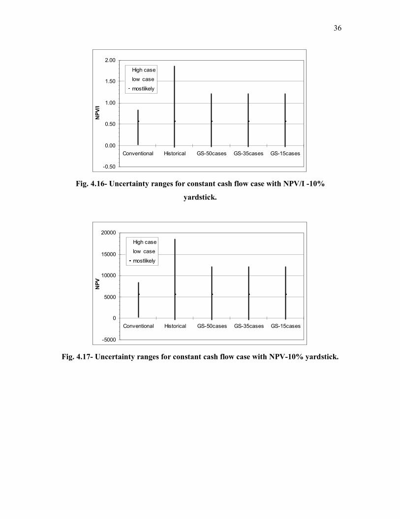
Fig. 4.10 to 4.18 show the ranges in investment evaluation yardsticks as

determined by conventional, historical and Gaussian simulation method. The ranges high

to low are much smaller for the conventional method than for the two methods based on

actual price histories. The cause of these discrepancies is that the conventional method

does not capture the short term volatility in prices that have actually occurred in the past.

TABLE 4.4 -- Ranges of Gaussian Simulation as Percentage of Historical Method.

Decreasing cash flow

case

Increasing cash flow

case

Constant cash flow

case Average IRR (%) 112% 65% 77% 85% NPV @5% ($) 86% 62% 66% 72% NPV @10% ($) 88% 60% 66% 71% NPV @15% ($) 89% 59% 66% 71% NPV/I @5% 87% 62% 67% 72% NPV/I @10% 88% 60% 68% 72% NPV/I @15% 89% 59% 89% 79%

Table 4.4 shows the ranges obtained from Gaussian simulation method calculated

as percentage of the ranges calculated for the historical method. The rate averages about

-12000

-10000

-8000

-6000

-4000

-2000

0

2000

4000

6000

8000

10000

0 1 2 3 4 5 6 7 8 9 10 11year

Cas

h Fl

ow ($

)

base 1 21

20 29 38

32

75%. The inability of G.S. method to capture the remaining 30% uncertainty can be

attributed to the underlying oil price histogram. In historical method as the scenarios are

built with respect to each year, every scenario has its own histogram which gives the

variability and effectively captures the uncertainty where as in G.S. method there is only

one histogram or price profile used to generate the 50 scenarios.

Fig. 4.10 to 4.18 show the ranges of investment evaluation yardsticks calculated

using conventional, historical and G.S. method. For the sensitivity analysis within G.S.

method three types of ranges are calculated that are based on underlying scenarios used.

To see the effectiveness of the method 15, 35 and 50 scenarios used to calculate the

maximum change in values of economic indicator or the range and then these ranges are

plotted on the stock market chart. The figures show that there is little difference in the

calculated ranges of certainty when we consider 15, 35 and 50 prediction scenarios. The

result indicates that 50 scenarios should be more that sufficient.

From the table we can make one more evident conclusion about the relation ship

between the ranges of uncertainty by G.S. method and that of historical method. Here in

the analysis we selected three projects having entirely different annual cash flow stream.

The table shows that G.S. method has obtained ranges greater than 85% of the historical

method for the decreasing project where as it predicts the 60% of the range for increasing

project. The constant project cash flow gives almost 68% of the range of historical

method. The variation in result of ranges with respect to cash flow stream suggests that

the method is dependant on the cash flow pattern and there exists high degree of

correlation for declining type of project among the both method.

33

Fig. 4.10- Uncertainty ranges for decreasing cash flow case with NPV/I -10%

yardstick.

Fig. 4.11- Uncertainty ranges for decreasing cash flow case with NPV-10%

yardstick.

-2000

0

2000

4000

6000

8000

10000

12000

14000

16000

18000

Conventional Historical GS-50cases GS-35cases GS-15cases

NPV

High case

low case

mostlikely

-0.20

0.00

0.20

0.40

0.60

0.80

1.00

1.20

1.40

1.60

1.80

Conventional Historical GS-50cases GS-35cases GS-15cases

NPV

/I

High case

low case

most-likely

34

Fig. 4.12- Uncertainty ranges for decreasing cash flow case with internal rate of

return yardstick.

Fig. 4.13- Uncertainty ranges for increasing cash flow case with NPV/I -10%

yardstick.

-0.50

0.00

0.50

1.00

1.50

2.00

2.50

3.00

3.50

Conventional Historical GS-50cases GS-35cases GS-15cases

NPV

/I

High case

low case

mostlikely

0%

10%

20%

30%

40%

50%

60%

70%

80%

Conventional Historical GS-50cases GS-35cases GS-15cases

IRR

High case

low case

mostlikely

35

Fig. 4.14- Uncertainty ranges for increasing cash flow case with NPV-10%

yardstick.

Fig. 4.15- Uncertainty ranges for increasing cash flow case with internal rate of

return yardstick.

0%

5%

10%

15%

20%

25%

30%

35%

Conventional Historical GS-50cases GS-35cases GS-15cases

IRR

High case

low case

mostlikely

-2000

0

2000

4000

6000

8000

10000

12000

14000

16000

18000

Conventional Historical GS-50cases GS-35cases GS-15cases

NPV

High case

low case

mostlikely

36

Fig. 4.16- Uncertainty ranges for constant cash flow case with NPV/I -10%

yardstick.

Fig. 4.17- Uncertainty ranges for constant cash flow case with NPV-10% yardstick.

-5000

0

5000

10000

15000

20000

Conventional Historical GS-50cases GS-35cases GS-15cases

NPV

High case

low case

mostlikely

-0.50

0.00

0.50

1.00

1.50

2.00

Conventional Historical GS-50cases GS-35cases GS-15cases

NPV

/I

High case

low case

mostlikely

37

Fig. 4.18- Uncertainty ranges for constant cash flow case with internal rate of return

yardstick.

Table 4.5 gives the ranges of uncertainty we obtained for the incremental

recovery case with conventional method and historical method. We note that the

uncertainty range obtained from the historical method is four times larger than that for the

conventional method. We also note that the use of our correlations of operating and

drilling costs with oil price .Therefore we can conclude from the results that the

conventional method of monotonic increase in price used to obtain future price range is

not sufficient to model the uncertainty as the analysis with the historical method that has

modeled the scenarios based on historical price profile starting from 1974 suggests there

is large uncertainty hiding which is outside of the scope of conventional method and use

of these methods will improve the uncertainty estimates and project selection capabilities

of the decision makers.

In Fig. 4.19, cumulative distribution function (CDF) is generated from the

historical method scenarios for the field case of incremental recovery using which P-10,

P-50, P-90 values can be calculated. Fig. 4.20 shows the uncertainty range on the stock

market chart obtained from table 4.5.

0%

5%

10%

15%

20%

25%

30%

35%

40%

45%

50%

Conventional Historical GS-50cases GS-35cases GS-15cases

IRR

High case

low case

mostlikely

38

TABLE 4.5 -- Uncertainty Range for Incremental Recovery Project.

NPV @12% Conventional Method Historical Method Conventional Method

No Correlation used

High Case $76,996,535 $193,459,369 $76,277,964 Low Case $49,769,343 $46,229,020 $50,124,589 Most Likely Case

$67,918,074 $67,918,074 $67,560,128

Range $27,227,192 $147,230,349 $26,153,374

Fig. 4.19- C.D.F. of incremental recovery case showing range of net present value.

Fig. 4.20- Uncertainty range comparison for incremental recovery case.

0.0

0.2

0.4

0.6

0.8

1.0

1.2

40 65 90 115 140 165 190

Bin (NPV-12%, MM$)

Prob

abili

ty

$0

$50

$100

$150

$200

$250

conventional w hencorrelation

historical conventional nocorrelationCases

NPV

12%

, MM

$

39

CHAPTER V

CONCLUSIONS AND FUTURE WORK

This research applied probabilistic and geostatistical technique to discounted cash flow

streams from representative petroleum projects to quantify the economic uncertainty. The

results for the model projects allow us to draw the following conclusions.

1. The ranges of uncertainty obtained from conventional analysis are very narrow

and are in consistent with that we observed for historical uncertainty ranges

captured by historical and Gaussian simulation (G.S.) method using the past three

decades oil price data.

2. The reason for the narrow ranges observed in conventional method is caused by

the methods exclusion of short period “shocks” or volatility in prices.

3. The historical method represents the observed economic uncertainty in past three

decades because it includes the price volatility that occurred for 1974 to 2002.

4. The G.S. method that we proposed has 70 per cent of the range of uncertainty

observed in historical method for the economic indicators we used in the study

reason being the histogram used for price modeling. The historical method uses

histograms generated with varying ranges from the past prices as compared to the

G.S. method that has only one underlying histogram.

5. The range of uncertainty produced by the G.S. method is dependant on cash flow

pattern as the percentage of range in terms of historical method varies from 59 to

almost 90%. For the project having declining cash flow pattern there is high

degree of correlation among the both methods compared to other two cash flow

patterns.

6. The sensitivity analysis for the G.S. method showed that the range of uncertainty

produced by 15 scenarios differs slightly for that produced by 35 scenarios and

that there was no further change when 50 prediction scenarios were considered.

7. The field case of incremental recovery using water and gas injection validates the

earlier conclusion that conventional method is not sufficient to model the

uncertainty as the ranges of uncertainty produced by conventional method and

historical method for NPV/I at 12% economic yardstick differ by almost 400%.

40

Future work could be directed at modifying the conventional method so that it accounts

for the price volatility. This might be achieved by using a statistical technique like

bootstrap3. The sensitivity of the system can be increased by daily spot price for historical

method than monthly average price. This change would generate thousands of scenarios

similar to the Monte Carlo simulation technique.

41

REFERENCES

1. Begg, S. and Bratvold, R.: “The Value of Flexibility in Managing Uncertainty in Oil

and Gas Investments,” paper SPE 77586 presented at the SPE Annual Technical

Conference and Exhibition, San Antonio, Texas, 29 September –2 October 2002.

2. Brashear, J.P., Becker, A.B. and Faulder, D.D.: “Where Have All the Profits Gone?

or Evaluating Risk and Returns of E&P projects,” paper SPE 63056 presented at the

SPE Annual Technical Conference and Exhibition, Dallas, Texas, 1- 4 October 2002.

3. McMichael, C.: “The Fallacy of Hockey Stick Projection,” paper SPE 56454

presented at the SPE Annual Technical Conference and Exhibition, Houston, Texas,

3-6 October 1999.

4. Kokolis, G.P., Litvak, B.L. and Rapp, W.J.: “Scenario Selection for Valuation of

Multiple Prospect Opportunities: A Monte Carlo Play Simulation Approach,” paper

SPE 52977 presented at SPE Hydrocarbon Economics and Evaluation Symposium,

Dallas, Texas, 20-23 March 1999.

5. Brashear, J.P., Becker, A.B. and Gabriel, S.A.: “Interdependencies Among E&P

Projects and Portfolio Risk Management,” paper SPE 56574 presented at the SPE

Annual Technical Conference and Exhibition, Houston, Texas, 3-6 October 1999.

6. Downes, J. and Goodman, J.E.: Dictionary of Finance and Investments Terms,

Hauppauge, Barron’s Educational Series, Inc., New York City (1995).

7. Dougherty, E.L. and Sarkar, J.: “Current Investment Practices and Procedures:

Results of a Survey of U.S. Oil and Gas Producers and Petroleum Consultants,” paper

SPE 25824 presented at SPE Hydrocarbon Economics and Evaluation Symposium,

Dallas, Texas, 29-30 March 1993.

8. Newendorp, P.: Decision Analysis for Petroleum Exploration, Pennwell Publishing

Co., Tulsa, Oklahoma (1975)

9. Caldwell, R. and Heather, D.: “Characterizing Uncertainty in Oil and Gas

Evaluations,” paper SPE 68592 presented at the SPE Hydrocarbon Economics and

Evaluation Symposium, Dallas, Texas, 2-3 April 2001.

42

10. Purvis, D.C.: “Judgment in Probabilistic Analysis,” paper SPE 81996 presented at

SPE Hydrocarbon Economics and Evaluation Symposium, Dallas, Texas, 5-8 April

2003.

11. Davidson, L.B.: “Practical Issues in Using Risk Based Decision Analysis,” paper SPE

71417 presented at the SPE Annual Technical Conference and Exhibition, New

Orleans, Louisiana, 30 September –3 October 2001.

12. Capen, E.C.: “The Difficulty of Assessing Uncertainty,” paper SPE 5579, JPT,

August 1976, XXVIII, 843-850.

13. Caldwell, R.H. and Heather, D.I.: “Why Our Reserves Definitions Don’t Work

Anymore,” paper SPE 30041 presented at SPE Hydrocarbon Economics and

Evaluation Symposium, Dallas, Texas, 26-28 March 1995.

14. Solomon, O.I., Kunju, M and Omowunmi, O.I.: “The Responsiveness of Global E&P

Industry to Changes in Petroleum Prices: Evidence From 1960-2000,” paper 68587

presented at SPE Hydrocarbon Economics and Evaluation Symposium, Dallas,

Texas, 2-3 April 2001.

15. Garb, F.A.: “Assessing Risk and Uncertainty in Evaluating Hydrocarbon Producing

Properties,” paper SPE 15921 presented at SPE Eastern Regional Meeting,

Columbus, Ohio, November 12-14, 1986.

16. Demirmen, F.: “Subsurface Appraisal: The Road from Reservoir Uncertainty to

Better Economics,” paper SPE 68603 presented at the SPE Hydrocarbon Economics

and Evaluation Symposium, Dallas, Texas, 2-3 April 2001.

17. Jain, P. and Raju, A.V.: “Evaluation of Economics and Technical Uncertainties for

Identification of Economic Volatility in Field Development and Asset Evaluation,”

paper SPE 39574 presented at 1998 SPE India Oil and Gas Conference and

Exhibition, New Delhi, 17-19 February.

18. Sadorsky, P., “Oil Price Shocks and Stock Market Activity”, Energy Economics.

21,449-469, (1999).

19. Edwards, R.A. and Hewett, T.A.: “Quantification of Production Uncertainty and Its

Impact on the Management of Oil and Gas Price Risk,” paper SPE 28330 presented at

69th SPE Annual Technical Conference and Exhibition, New Orleans, Louisiana, 25-

28 September 1994.

43

20. Castro, G.T., Bordalo, S.N. and Morooka C.K.: “Decision-Making Process for a

Deepwater Production System Considering Environmental, Technological and

Financial Risks,” paper SPE 77423 presented at the SPE Annual Technical

Conference and Exhibition, San Antonio, Texas, 29 September –2 October 2002.

21. Cabedo, J.D. and Moya I.: “Estimating Oil Price ‘Value at Risk’ using the Historical

Simulation Approach,” Energy Economics, 25, 239-253 (2003).

22. Behrens, A.M. and Choobineh, F.F.: “An Alternative Approach to Modeling

Uncertainty in Hydrocarbon Economic Analysis,” paper SPE 25838 presented at SPE

Hydrocarbon Economics and Evaluation Symposium, Dallas, Texas, 29-30 March

1993.

23. Jensen, J.L., Corbett, W.M., Lake, L.W. and Goggin, D.J.: “Statistics for Petroleum

Engineers and Geoscientists”, Elsevier Science B.V., Amsterdam, Netherlands

(2000).

24. Deutsch, C.V. and Journel, A.G.: “GSLIB Geostatistical Software Library and User’s

Guide”, Oxford University Press, New York (1992).

25. “U.S. Crude Oil Daily Spot Prices,” Energy Information Administration, Department

of Energy, http://www.eia.doe.gov/neic/historic/hpetroleum2.htm#CrudeOil (Feb’03).

26. “Consumer Price Index for All Urban Consumers: All Items,” U.S. Department of

Labor: Bureau of Labor Statistics, http://stats.bls.gov:80/opub/hom/homch17_itc.htm

(Feb’03)

27. “Joint Association on Drilling Cost for Year 1970 to 1984, Drilling Expenditure for

Oil, Gas and Dry Wells” Energy Statistics Handbook Edition 13, PennWell

Publications, Tulsa (1999).

28. “Historical Production Prices,” Energy Information Administration, Department of

Energy,http://www.eia.doe.gov/oil_gas/natural_gas/data_publications/cost_indices/c_

i.html (Feb’03)

29. Seba, R.D.: Economics of Worldwide Petroleum Production, OGCI Publications,

Tulsa, Oklahoma (1998).

30. Capen, E.C., Clapp, R.V. and Phelps, W.W.: “Growth Rate: A Rate-of-Return

Measure of Investment Efficiency,” SPE 4613, JPT, (March 1976), XXVIII, 531-

543.

44

APPENDIX A

Table A-1 gives WTI crude price with the CPI index data used in this research. The

following columns describe the values derived from this data to use in methods used in

research. The inflation index column for year 1974 is derived from CPI data by

normalizing it with January 1974. To give a comparison between deflated price and

actual price the next column of deflated oil price is generated using the 1974 inflation

index column. The average inflation index is derived analyzing the CPI data the

procedure is explained in Appendix B. The historical method uses the average inflated

price indices these price profile is generated using the deflated oil price and average

inflation index over here we show the average inflation price profile for year 1974.

TABLE A.1- Historical Oil Price and Inflation Indices.

Month

Actual Oil Price ($/STB)

C.P.I. Index

Inflation Index for 1974=1.0

Deflated Oil Price 1974 =6.95

Average Inflation Index

Average Inflated Price ($/STB)

0 Jan-74 6.95 46.6 1.0000 6.95 1.0000 6.95 1 Feb-74 6.87 47.2 1.0129 6.78 1.0039 6.81 2 Mar-74 6.77 47.8 1.0258 6.60 1.0078 6.65 3 Apr-74 6.77 48.0 1.0300 6.57 1.0118 6.65 4 May-74 6.87 48.6 1.0429 6.59 1.0158 6.69 5 Jun-74 6.85 49.0 1.0515 6.51 1.0197 6.64 6 Jul-74 6.80 49.4 1.0601 6.41 1.0237 6.57 7 Aug-74 6.71 50.0 1.0730 6.25 1.0277 6.43 8 Sep-74 6.70 50.6 1.0858 6.17 1.0318 6.37 9 Oct-74 6.97 51.1 1.0966 6.36 1.0358 6.58

10 Nov-74 6.97 51.5 1.1052 6.31 1.0399 6.56 11 Dec-74 7.09 51.9 1.1137 6.37 1.0439 6.65 12 Jan-75 7.61 52.1 1.1180 6.81 1.0480 7.13 13 Feb-75 7.47 52.5 1.1266 6.63 1.0521 6.98 14 Mar-75 7.57 52.7 1.1309 6.69 1.0562 7.07 15 Apr-75 7.55 52.9 1.1352 6.65 1.0604 7.05 16 May-75 7.52 53.2 1.1416 6.59 1.0645 7.01 17 Jun-75 7.49 53.6 1.1502 6.51 1.0687 6.96 18 Jul-75 7.75 54.2 1.1631 6.66 1.0729 7.15 19 Aug-75 7.73 54.3 1.1652 6.63 1.0771 7.15

45

20 Sep-75 7.75 54.6 1.1717 6.61 1.0813 7.15

Month

Actual Oil Price ($/STB)

C.P.I. Index

Inflation Index for 1974=1.0

Deflated Oil Price 1974

=6.95

Average Inflation

Index

Average Inflated

Price ($/STB)

21 Oct-75 7.83 54.9 1.1781 6.65 1.0855 7.21 22 Nov-75 7.80 55.3 1.1867 6.57 1.0898 7.16 23 Dec-75 7.93 55.5 1.1910 6.66 1.0941 7.28 24 Jan-76 8.63 55.6 1.1931 7.23 1.0984 7.94 25 Feb-76 7.87 55.8 1.1974 6.57 1.1027 7.25 26 Mar-76 7.79 55.9 1.1996 6.49 1.1070 7.19 27 Apr-76 7.86 56.1 1.2039 6.53 1.1113 7.26 28 May-76 7.89 56.5 1.2124 6.51 1.1157 7.26 29 Jun-76 7.99 56.8 1.2189 6.56 1.1200 7.34 30 Jul-76 8.04 57.1 1.2253 6.56 1.1244 7.38 31 Aug-76 8.03 57.4 1.2318 6.52 1.1288 7.36 32 Sep-76 8.39 57.6 1.2361 6.79 1.1332 7.69 33 Oct-76 8.46 57.9 1.2425 6.81 1.1377 7.75 34 Nov-76 8.62 58.0 1.2446 6.93 1.1421 7.91 35 Dec-76 8.62 58.2 1.2489 6.90 1.1466 7.91 36 Jan-77 8.50 58.5 1.2554 6.77 1.1511 7.79 37 Feb-77 8.57 59.1 1.2682 6.76 1.1556 7.81 38 Mar-77 8.45 59.5 1.2768 6.62 1.1601 7.68 39 Apr-77 8.40 60.0 1.2876 6.52 1.1647 7.60 40 May-77 8.49 60.3 1.2940 6.56 1.1692 7.67 41 Jun-77 8.44 60.7 1.3026 6.48 1.1738 7.61 42 Jul-77 8.48 61.0 1.3090 6.48 1.1784 7.63 43 Aug-77 8.62 61.2 1.3133 6.56 1.1830 7.76 44 Sep-77 8.63 61.4 1.3176 6.55 1.1877 7.78 45 Oct-77 8.72 61.6 1.3219 6.60 1.1923 7.87 46 Nov-77 8.72 61.9 1.3283 6.56 1.1970 7.86 47 Dec-77 8.77 62.1 1.3326 6.58 1.2017 7.91 48 Jan-78 8.68 62.5 1.3412 6.47 1.2064 7.81 49 Feb-78 8.84 62.9 1.3498 6.55 1.2111 7.93 50 Mar-78 8.80 63.4 1.3605 6.47 1.2158 7.86 51 Apr-78 8.82 63.9 1.3712 6.43 1.2206 7.85 52 May-78 8.81 64.5 1.3841 6.37 1.2254 7.80 53 Jun-78 9.05 65.2 1.3991 6.47 1.2302 7.96 54 Jul-78 8.96 65.7 1.4099 6.36 1.2350 7.85 55 Aug-78 9.05 66.0 1.4163 6.39 1.2398 7.92 56 Sep-78 9.15 66.5 1.4270 6.41 1.2447 7.98 57 Oct-78 9.17 67.1 1.4399 6.37 1.2496 7.96 58 Nov-78 9.20 67.4 1.4464 6.36 1.2545 7.98

46

59 Dec-78 9.47 67.7 1.4528 6.52 1.2594 8.21

Month

Actual Oil Price ($/STB)

C.P.I. Index

Inflation Index for 1974=1.0

Deflated Oil Price 1974

=6.95

Average Inflation

Index

Average Inflated

Price ($/STB)

60 Jan-79 9.46 68.3 1.4657 6.45 1.2643 8.16 61 Feb-79 9.69 69.1 1.4828 6.53 1.2693 8.29 62 Mar-79 9.83 69.8 1.4979 6.56 1.2742 8.36 63 Apr-79 10.33 70.6 1.5150 6.82 1.2792 8.72 64 May-79 10.71 71.5 1.5343 6.98 1.2842 8.96 65 Jun-79 11.70 72.3 1.5515 7.54 1.2893 9.72 66 Jul-79 13.39 73.1 1.5687 8.54 1.2943 11.05 67 Aug-79 14.00 73.8 1.5837 8.84 1.2994 11.49 68 Sep-79 14.57 74.6 1.6009 9.10 1.3045 11.87 69 Oct-79 15.11 75.2 1.6137 9.36 1.3096 12.26 70 Nov-79 15.52 75.9 1.6288 9.53 1.3147 12.53 71 Dec-79 17.03 76.7 1.6459 10.35 1.3199 13.66 72 Jan-80 17.86 77.8 1.6695 10.70 1.3250 14.17 73 Feb-80 18.81 78.9 1.6931 11.11 1.3302 14.78 74 Mar-80 19.34 80.1 1.7189 11.25 1.3354 15.03 75 Apr-80 20.29 81.0 1.7382 11.67 1.3407 15.65 76 May-80 21.01 81.8 1.7554 11.97 1.3459 16.11 77 Jun-80 21.53 82.7 1.7747 12.13 1.3512 16.39 78 Jul-80 22.26 82.7 1.7747 12.54 1.3565 17.01 79 Aug-80 22.63 83.3 1.7876 12.66 1.3618 17.24 80 Sep-80 22.59 84.0 1.8026 12.53 1.3671 17.13 81 Oct-80 23.23 84.8 1.8197 12.77 1.3725 17.52 82 Nov-80 23.92 85.5 1.8348 13.04 1.3778 17.96 83 Dec-80 25.80 86.3 1.8519 13.93 1.3832 19.27 84 Jan-81 28.85 87.0 1.8670 15.45 1.3887 21.46 85 Feb-81 34.14 87.9 1.8863 18.10 1.3941 25.23 86 Mar-81 34.70 88.5 1.8991 18.27 1.3996 25.57 87 Apr-81 34.05 89.1 1.9120 17.81 1.4050 25.02 88 May-81 32.71 89.8 1.9270 16.97 1.4105 23.94 89 Jun-81 31.71 90.6 1.9442 16.31 1.4161 23.10 90 Jul-81 31.13 91.6 1.9657 15.84 1.4216 22.51 91 Aug-81 31.13 92.3 1.9807 15.72 1.4272 22.43 92 Sep-81 31.13 93.2 2.0000 15.57 1.4328 22.30 93 Oct-81 31.00 93.4 2.0043 15.47 1.4384 22.25 94 Nov-81 30.98 93.7 2.0107 15.41 1.4440 22.25 95 Dec-81 30.72 94.0 2.0172 15.23 1.4497 22.08 96 Jan-82 33.85 94.3 2.0236 16.73 1.4553 24.34 97 Feb-82 31.56 94.6 2.0300 15.55 1.4610 22.71

47

98 Mar-82 28.48 94.5 2.0279 14.04 1.4668 20.60

Month

Actual Oil Price ($/STB)

C.P.I. Index

Inflation Index for 1974=1.0

Deflated Oil Price 1974

=6.95

Average Inflation

Index

Average Inflated

Price ($/STB)

99 Apr-82 33.45 94.9 2.0365 16.43 1.4725 24.19 100 May-82 35.93 95.8 2.0558 17.48 1.4783 25.84 101 Jun-82 35.07 97.0 2.0815 16.85 1.4841 25.00 102 Jul-82 34.16 97.5 2.0923 16.33 1.4899 24.32 103 Aug-82 33.95 97.7 2.0966 16.19 1.4957 24.22 104 Sep-82 35.63 97.9 2.1009 16.96 1.5016 25.47 105 Oct-82 35.68 98.2 2.1073 16.93 1.5075 25.52 106 Nov-82 34.15 98.0 2.1030 16.24 1.5134 24.57 107 Dec-82 31.70 97.6 2.0944 15.14 1.5193 23.00 108 Jan-83 31.19 97.8 2.0987 14.86 1.5252 22.67 109 Feb-83 28.95 97.9 2.1009 13.78 1.5312 21.10 110 Mar-83 28.62 97.9 2.1009 13.62 1.5372 20.94 111 Apr-83 30.61 98.6 2.1159 14.47 1.5432 22.33 112 May-83 30.00 99.2 2.1288 14.09 1.5493 21.83 113 Jun-83 31.00 99.5 2.1352 14.52 1.5553 22.58 114 Jul-83 31.66 99.9 2.1438 14.77 1.5614 23.06 115 Aug-83 31.91 100.2 2.1502 14.84 1.5675 23.26 116 Sep-83 31.11 100.7 2.1609 14.40 1.5737 22.66 117 Oct-83 30.41 101.0 2.1674 14.03 1.5798 22.17 118 Nov-83 29.84 101.2 2.1717 13.74 1.5860 21.79 119 Dec-83 29.24 101.3 2.1738 13.45 1.5922 21.42 120 Jan-84 29.74 101.9 2.1867 13.60 1.5985 21.74 121 Feb-84 30.20 102.4 2.1974 13.74 1.6047 22.05 122 Mar-84 30.76 102.6 2.2017 13.97 1.6110 22.51 123 Apr-84 30.60 103.1 2.2124 13.83 1.6173 22.37 124 May-84 30.67 103.4 2.2189 13.82 1.6237 22.44 125 Jun-84 29.86 103.7 2.2253 13.42 1.6300 21.87 126 Jul-84 28.71 104.1 2.2339 12.85 1.6364 21.03 127 Aug-84 29.22 104.5 2.2425 13.03 1.6428 21.41 128 Sep-84 29.38 105.0 2.2532 13.04 1.6493 21.50 129 Oct-84 28.58 105.3 2.2597 12.65 1.6557 20.94 130 Nov-84 27.99 105.3 2.2597 12.39 1.6622 20.59 131 Dec-84 26.65 105.3 2.2597 11.79 1.6687 19.68 132 Jan-85 25.85 105.5 2.2639 11.42 1.6752 19.13 133 Feb-85 27.33 106.0 2.2747 12.01 1.6818 20.21 134 Mar-85 28.53 106.4 2.2833 12.50 1.6884 21.10 135 Apr-85 28.60 106.9 2.2940 12.47 1.6950 21.13 136 May-85 27.61 107.3 2.3026 11.99 1.7016 20.40

48

137 Jun-85 27.14 107.6 2.3090 11.75 1.7083 20.08

Month

Actual Oil Price ($/STB)

C.P.I. Index

Inflation Index for 1974=1.0

Deflated Oil Price 1974

=6.95

Average Inflation

Index

Average Inflated

Price ($/STB)

138 Jul-85 27.23 107.8 2.3133 11.77 1.7150 20.19 139 Aug-85 27.58 108.0 2.3176 11.90 1.7217 20.49 140 Sep-85 28.53 108.3 2.3240 12.28 1.7285 21.22 141 Oct-85 29.54 108.7 2.3326 12.66 1.7352 21.97 142 Nov-85 30.90 109.0 2.3391 13.21 1.7420 23.01 143 Dec-85 27.46 109.3 2.3455 11.71 1.7488 20.47 144 Jan-86 22.93 109.6 2.3519 9.75 1.7557 17.12 145 Feb-86 15.45 109.3 2.3455 6.59 1.7626 11.61 146 Mar-86 12.61 108.8 2.3348 5.40 1.7695 9.56 147 Apr-86 12.84 108.6 2.3305 5.51 1.7764 9.79 148 May-86 15.38 108.9 2.3369 6.58 1.7834 11.74 149 Jun-86 13.43 109.5 2.3498 5.71 1.7903 10.23 150 Jul-86 11.58 109.5 2.3498 4.93 1.7974 8.86 151 Aug-86 15.10 109.7 2.3541 6.41 1.8044 11.57 152 Sep-86 14.87 110.2 2.3648 6.29 1.8115 11.39 153 Oct-86 14.90 110.3 2.3670 6.29 1.8186 11.45 154 Nov-86 15.22 110.4 2.3691 6.43 1.8257 11.73 155 Dec-86 16.11 110.5 2.3712 6.79 1.8328 12.45 156 Jan-87 18.65 111.2 2.3863 7.82 1.8400 14.38 157 Feb-87 17.75 111.6 2.3948 7.41 1.8472 13.69 158 Mar-87 18.30 112.1 2.4056 7.61 1.8544 14.11 159 Apr-87 18.68 112.7 2.4185 7.72 1.8617 14.38 160 May-87 19.44 113.1 2.4270 8.01 1.8690 14.97 161 Jun-87 20.07 113.5 2.4356 8.24 1.8763 15.46 162 Jul-87 21.34 113.8 2.4421 8.74 1.8837 16.46 163 Aug-87 20.31 114.4 2.4549 8.27 1.8910 15.65 164 Sep-87 19.53 115.0 2.4678 7.91 1.8985 15.02 165 Oct-87 19.86 115.3 2.4742 8.03 1.9059 15.30 166 Nov-87 18.85 115.4 2.4764 7.61 1.9134 14.57 167 Dec-87 17.27 115.4 2.4764 6.98 1.9208 13.40 168 Jan-88 17.13 115.7 2.4828 6.90 1.9284 13.30 169 Feb-88 16.80 116.0 2.4893 6.75 1.9359 13.06 170 Mar-88 16.20 116.5 2.5000 6.48 1.9435 12.59 171 Apr-88 17.86 117.1 2.5129 7.11 1.9511 13.87 172 May-88 17.42 117.5 2.5215 6.91 1.9588 13.54 173 Jun-88 16.53 118.0 2.5322 6.53 1.9664 12.83 174 Jul-88 15.50 118.5 2.5429 6.09 1.9741 12.03 175 Aug-88 15.52 119.0 2.5536 6.08 1.9819 12.05

49

176 Sep-88 14.54 119.8 2.5708 5.65 1.9896 11.25

Month

Actual Oil Price ($/STB)

C.P.I. Index

Inflation Index for 1974=1.0

Deflated Oil Price 1974

=6.95

Average Inflation

Index

Average Inflated

Price ($/STB)

177 Oct-88 13.77 120.2 2.5794 5.34 1.9974 10.66 178 Nov-88 14.14 120.3 2.5815 5.48 2.0052 10.98 179 Dec-88 16.38 120.5 2.5858 6.34 2.0131 12.75 180 Jan-89 18.02 121.1 2.5987 6.94 2.0210 14.02 181 Feb-89 17.94 121.6 2.6094 6.87 2.0289 13.95 182 Mar-89 19.48 122.3 2.6245 7.42 2.0368 15.12 183 Apr-89 21.07 123.1 2.6416 7.98 2.0448 16.31 184 May-89 20.12 123.8 2.6567 7.57 2.0528 15.55 185 Jun-89 20.05 124.1 2.6631 7.53 2.0609 15.52 186 Jul-89 19.78 124.4 2.6695 7.41 2.0689 15.33 187 Aug-89 18.58 124.6 2.6738 6.95 2.0770 14.43 188 Sep-89 19.59 125.0 2.6824 7.30 2.0852 15.23 189 Oct-89 20.10 125.6 2.6953 7.46 2.0933 15.61 190 Nov-89 19.86 125.9 2.7017 7.35 2.1015 15.44 191 Dec-89 21.10 126.1 2.7060 7.80 2.1098 16.45 192 Jan-90 22.86 127.4 2.7339 8.36 2.1180 17.71 193 Feb-90 22.11 128.0 2.7468 8.05 2.1263 17.12 194 Mar-90 20.39 128.7 2.7618 7.38 2.1346 15.76 195 Apr-90 18.43 128.9 2.7661 6.66 2.1430 14.27 196 May-90 18.20 129.2 2.7725 6.56 2.1514 14.12 197 Jun-90 16.70 129.9 2.7876 5.99 2.1598 12.94 198 Jul-90 18.45 130.4 2.7983 6.59 2.1683 14.30 199 Aug-90 27.31 131.6 2.8240 9.67 2.1768 21.05 200 Sep-90 33.51 132.7 2.8476 11.77 2.1853 25.71 201 Oct-90 36.04 133.5 2.8648 12.58 2.1939 27.60 202 Nov-90 32.33 133.8 2.8712 11.26 2.2025 24.80 203 Dec-90 27.28 133.8 2.8712 9.50 2.2111 21.01 204 Jan-91 25.23 134.6 2.8884 8.73 2.2197 19.39 205 Feb-91 20.48 134.8 2.8927 7.08 2.2284 15.78 206 Mar-91 19.90 135.0 2.8970 6.87 2.2372 15.37 207 Apr-91 20.83 135.2 2.9013 7.18 2.2459 16.12 208 May-91 21.23 135.6 2.9099 7.30 2.2547 16.45 209 Jun-91 20.19 136.0 2.9185 6.92 2.2635 15.66 210 Jul-91 21.40 136.2 2.9227 7.32 2.2724 16.64 211 Aug-91 21.69 136.6 2.9313 7.40 2.2813 16.88 212 Sep-91 21.89 137.2 2.9442 7.43 2.2902 17.03 213 Oct-91 23.23 137.4 2.9485 7.88 2.2992 18.11 214 Nov-91 22.46 137.8 2.9571 7.60 2.3082 17.53

50

215 Dec-91 19.50 137.9 2.9592 6.59 2.3173 15.27

Month

Actual Oil Price ($/STB)

C.P.I. Index

Inflation Index for 1974=1.0

Deflated Oil Price 1974

=6.95

Average Inflation

Index

Average Inflated

Price ($/STB)

216 Jan-92 18.79 138.1 2.9635 6.34 2.3263 14.75 217 Feb-92 19.01 138.6 2.9742 6.39 2.3354 14.93 218 Mar-92 18.92 139.3 2.9893 6.33 2.3446 14.84 219 Apr-92 20.23 139.5 2.9936 6.76 2.3538 15.91 220 May-92 20.98 139.7 2.9979 7.00 2.3630 16.54 221 Jun-92 22.38 140.2 3.0086 7.44 2.3722 17.65 222 Jul-92 21.77 140.5 3.0150 7.22 2.3815 17.20 223 Aug-92 21.34 140.9 3.0236 7.06 2.3909 16.87 224 Sep-92 21.88 141.3 3.0322 7.22 2.4002 17.32 225 Oct-92 21.69 141.8 3.0429 7.13 2.4096 17.18 226 Nov-92 20.34 142.0 3.0472 6.67 2.4191 16.15 227 Dec-92 19.41 141.9 3.0451 6.37 2.4285 15.48 228 Jan-93 19.03 142.6 3.0601 6.22 2.4381 15.16 229 Feb-93 20.09 143.1 3.0708 6.54 2.4476 16.01 230 Mar-93 20.32 143.6 3.0815 6.59 2.4572 16.20 231 Apr-93 20.25 144.0 3.0901 6.55 2.4668 16.17 232 May-93 19.95 144.2 3.0944 6.45 2.4765 15.97 233 Jun-93 19.09 144.4 3.0987 6.16 2.4862 15.32 234 Jul-93 17.89 144.4 3.0987 5.77 2.4959 14.41 235 Aug-93 18.01 144.8 3.1073 5.80 2.5057 14.52 236 Sep-93 18.09 145.1 3.1137 5.81 2.5155 14.61 237 Oct-93 18.15 145.7 3.1266 5.81 2.5253 14.66 238 Nov-93 16.61 145.8 3.1288 5.31 2.5352 13.46 239 Dec-93 14.51 145.8 3.1288 4.64 2.5452 11.80 240 Jan-94 15.03 146.2 3.1373 4.79 2.5551 12.24 241 Feb-94 14.78 146.7 3.1481 4.69 2.5651 12.04 242 Mar-94 14.68 147.2 3.1588 4.65 2.5752 11.97 243 Apr-94 16.42 147.4 3.1631 5.19 2.5853 13.42 244 May-94 17.89 147.5 3.1652 5.65 2.5954 14.67 245 Jun-94 19.06 148.0 3.1760 6.00 2.6056 15.64 246 Jul-94 19.65 148.4 3.1845 6.17 2.6158 16.14 247 Aug-94 18.38 149.0 3.1974 5.75 2.6260 15.10 248 Sep-94 17.45 149.4 3.2060 5.44 2.6363 14.35 249 Oct-94 17.72 149.5 3.2082 5.52 2.6466 14.62 250 Nov-94 18.07 149.7 3.2124 5.62 2.6570 14.95 251 Dec-94 17.16 149.7 3.2124 5.34 2.6674 14.25 252 Jan-95 18.04 150.3 3.2253 5.59 2.6778 14.98 253 Feb-95 18.57 150.9 3.2382 5.73 2.6883 15.42

51

254 Mar-95 18.54 151.4 3.2489 5.71 2.6989 15.40

Month

Actual Oil Price ($/STB)

C.P.I. Index

Inflation Index for 1974=1.0

Deflated Oil Price 1974

=6.95

Average Inflation

Index

Average Inflated

Price ($/STB)

255 Apr-95 19.90 151.9 3.2597 6.10 2.7094 16.54 256 May-95 19.74 152.2 3.2661 6.04 2.7200 16.44 257 Jun-95 18.45 152.5 3.2725 5.64 2.7307 15.40 258 Jul-95 17.33 152.5 3.2725 5.30 2.7414 14.52 259 Aug-95 18.02 152.9 3.2811 5.49 2.7521 15.11 260 Sep-95 18.23 153.2 3.2876 5.55 2.7629 15.32 261 Oct-95 17.43 153.7 3.2983 5.28 2.7737 14.66 262 Nov-95 17.99 153.6 3.2961 5.46 2.7846 15.20 263 Dec-95 19.03 153.5 3.2940 5.78 2.7955 16.15 264 Jan-96 18.85 154.4 3.3133 5.69 2.8064 15.97 265 Feb-96 19.09 154.9 3.3240 5.74 2.8174 16.18 266 Mar-96 21.33 155.7 3.3412 6.38 2.8285 18.06 267 Apr-96 23.50 156.3 3.3541 7.01 2.8395 19.89 268 May-96 21.17 156.6 3.3605 6.30 2.8507 17.96 269 Jun-96 20.42 156.7 3.3627 6.07 2.8618 17.38 270 Jul-96 21.30 157.0 3.3691 6.32 2.8730 18.16 271 Aug-96 21.90 157.3 3.3755 6.49 2.8843 18.71 272 Sep-96 23.97 157.8 3.3863 7.08 2.8956 20.50 273 Oct-96 24.88 158.3 3.3970 7.32 2.9069 21.29 274 Nov-96 23.71 158.6 3.4034 6.97 2.9183 20.33 275 Dec-96 25.22 158.6 3.4034 7.41 2.9297 21.71 276 Jan-97 25.13 159.1 3.4142 7.36 2.9412 21.65 277 Feb-97 22.18 159.6 3.4249 6.48 2.9527 19.12 278 Mar-97 20.97 160.0 3.4335 6.11 2.9643 18.10 279 Apr-97 19.70 160.2 3.4378 5.73 2.9759 17.05 280 May-97 20.82 160.1 3.4356 6.06 2.9876 18.10 281 Jun-97 19.26 160.3 3.4399 5.60 2.9993 16.79 282 Jul-97 19.66 160.5 3.4442 5.71 3.0110 17.19 283 Aug-97 19.95 160.8 3.4506 5.78 3.0228 17.48 284 Sep-97 19.80 161.2 3.4592 5.72 3.0346 17.37 285 Oct-97 21.33 161.6 3.4678 6.15 3.0465 18.74 286 Nov-97 20.19 161.5 3.4657 5.83 3.0585 17.82 287 Dec-97 18.33 161.3 3.4614 5.30 3.0704 16.26 288 Jan-98 16.72 161.6 3.4678 4.82 3.0825 14.86 289 Feb-98 16.06 161.9 3.4742 4.62 3.0945 14.30 290 Mar-98 15.12 162.2 3.4807 4.34 3.1066 13.50 291 Apr-98 15.35 162.5 3.4871 4.40 3.1188 13.73 292 May-98 14.91 162.8 3.4936 4.27 3.1310 13.36

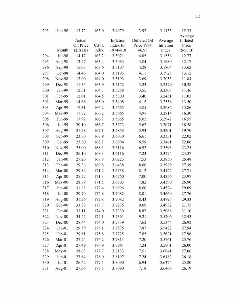
52

293 Jun-98 13.72 163.0 3.4979 3.92 3.1433 12.33

Month

Actual Oil Price ($/STB)

C.P.I. Index

Inflation Index for 1974=1.0

Deflated Oil Price 1974

=6.95

Average Inflation

Index

Average Inflated

Price ($/STB)

294 Jul-98 14.17 163.2 3.5021 4.05 3.1556 12.77 295 Aug-98 13.47 163.4 3.5064 3.84 3.1680 12.17 296 Sep-98 15.03 163.6 3.5107 4.28 3.1804 13.62 297 Oct-98 14.46 164.0 3.5193 4.11 3.1928 13.12 298 Nov-98 13.00 164.0 3.5193 3.69 3.2053 11.84 299 Dec-98 11.35 163.9 3.5172 3.23 3.2179 10.38 300 Jan-99 12.51 164.3 3.5258 3.55 3.2305 11.46 301 Feb-99 12.01 164.5 3.5300 3.40 3.2431 11.03 302 Mar-99 14.68 165.0 3.5408 4.15 3.2558 13.50 303 Apr-99 17.31 166.2 3.5665 4.85 3.2686 15.86 304 May-99 17.72 166.2 3.5665 4.97 3.2814 16.30 305 Jun-99 17.92 166.2 3.5665 5.02 3.2942 16.55 306 Jul-99 20.10 166.7 3.5773 5.62 3.3071 18.58 307 Aug-99 21.28 167.1 3.5858 5.93 3.3201 19.70 308 Sep-99 23.80 167.9 3.6030 6.61 3.3331 22.02 309 Oct-99 23.80 168.2 3.6094 6.59 3.3461 22.06 310 Nov-99 25.00 168.3 3.6116 6.92 3.3593 23.25 311 Dec-99 26.10 168.3 3.6116 7.23 3.3724 24.37 312 Jan-00 27.26 168.8 3.6223 7.53 3.3856 25.48 313 Feb-00 29.36 169.8 3.6438 8.06 3.3989 27.39 314 Mar-00 29.84 171.2 3.6738 8.12 3.4122 27.71 315 Apr-00 25.72 171.3 3.6760 7.00 3.4256 23.97 316 May-00 28.79 171.5 3.6803 7.82 3.4390 26.90 317 Jun-00 31.82 172.4 3.6996 8.60 3.4524 29.69 318 Jul-00 29.70 172.8 3.7082 8.01 3.4660 27.76 319 Aug-00 31.26 172.8 3.7082 8.43 3.4795 29.33 320 Sep-00 33.88 173.7 3.7275 9.09 3.4932 31.75 321 Oct-00 33.11 174.0 3.7339 8.87 3.5068 31.10 322 Nov-00 34.42 174.1 3.7361 9.21 3.5206 32.43 323 Dec-00 28.44 174.0 3.7339 7.62 3.5344 26.92 324 Jan-01 29.59 175.1 3.7575 7.87 3.5482 27.94 325 Feb-01 29.61 175.8 3.7725 7.85 3.5621 27.96 326 Mar-01 27.24 176.2 3.7811 7.20 3.5761 25.76 327 Apr-01 27.49 176.9 3.7961 7.24 3.5901 26.00 328 May-01 28.63 177.7 3.8133 7.51 3.6041 27.06 329 Jun-01 27.64 178.0 3.8197 7.24 3.6182 26.18 330 Jul-01 26.42 177.5 3.8090 6.94 3.6324 25.20 331 Aug-01 27.36 177.5 3.8090 7.18 3.6466 26.19

53

332 Sep-01 26.21 178.3 3.8262 6.85 3.6609 25.08

Month

Actual Oil Price ($/STB)

C.P.I. Index

Inflation Index for 1974=1.0

Deflated Oil Price 1974

=6.95

Average Inflation

Index

Average Inflated

Price ($/STB)

333 Oct-01 22.18 177.7 3.8133 5.82 3.6752 21.38 334 Nov-01 19.80 177.4 3.8069 5.20 3.6896 19.19 335 Dec-01 19.39 176.7 3.7918 5.11 3.7041 18.94 336 Jan-02 19.71 177.1 3.8004 5.19 3.7186 19.29 337 Feb-02 20.72 177.8 3.8155 5.43 3.7332 20.27 338 Mar-02 24.53 178.8 3.8369 6.39 3.7478 23.96 339 Apr-02 26.18 179.8 3.8584 6.79 3.7625 25.53 340 May-02 27.04 179.8 3.8584 7.01 3.7772 26.47 341 Jun-02 25.52 179.9 3.8605 6.61 3.7920 25.07 342 Jul-02 26.97 180.1 3.8648 6.98 3.8068 26.57 343 Aug-02 28.39 180.7 3.8777 7.32 3.8217 27.98 344 Sep-02 29.66 181.0 3.8841 7.64 3.8367 29.30 345 Oct-02 28.84 181.3 3.8906 7.41 3.8517 28.55 346 Nov-02 26.35 181.3 3.8906 6.77 3.8668 26.19 347 Dec-02 29.46 180.9 3.8820 7.59 3.8820 29.46

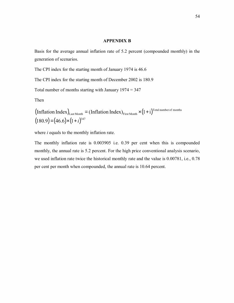
54

APPENDIX B

Basis for the average annual inflation rate of 5.2 percent (compounded monthly) in the

generation of scenarios.

The CPI index for the starting month of January 1974 is 46.6

The CPI index for the starting month of December 2002 is 180.9

Total number of months starting with January 1974 = 347

Then

( ) ( )( ) ( ) ( )347

months ofnumber TotalMonthFirst MonthLast

16.469.180

i1Index)Inflation (IndexInflation

i+×=

+×=

where i equals to the monthly inflation rate.

The monthly inflation rate is 0.003905 i.e. 0.39 per cent when this is compounded

monthly, the annual rate is 5.2 percent. For the high price conventional analysis scenario,

we used inflation rate twice the historical monthly rate and the value is 0.00781, i.e., 0.78

per cent per month when compounded, the annual rate is 10.64 percent.

55

VITA

Ashish Mendjoge received his B.E. degree in petroleum engineering from Maharashtra

Institute of Technology, University of Pune, in July 2000. Prior to joining TAMU he

worked with the Maharashtra Institute of Technology as a research engineer on the “Oil

spill contingency management using geographic information system” project. His

experience at TAMU includes working as a research assistant in the Reservoir

Uncertainty group with Dr. W.J. Lee and Dr. D.A. McVay.

Address: Texas A&M University

Attn: Dr. W.J. Lee

Harold Vance Department of Petroleum Engineering

3116 TAMU

College Station, TX 77843-3116