Estimating the Economic Impacts of Multimodal ...€¦ · state highway administration research...
59
STATE HIGHWAY ADMINISTRATION RESEARCH REPORT ESTIMATING THE ECONOMIC IMPACTS OF MULTIMODAL TRANSPORTATION IMPROVEMENTS PRINCIPAL INVESTIGATORS Lei Zhang Paul Schonfeld GRADUATE RESEARCH ASSISTANTS Eirini Kastrouni Elham Shayanfar Xiang He UNIVERSITY OF MARYLAND SP409B4M FINAL REPORT February 2016 MD-16-SHA-UM-3-17
Transcript of Estimating the Economic Impacts of Multimodal ...€¦ · state highway administration research...

STATE HIGHWAY ADMINISTRATION
RESEARCH REPORT
ESTIMATING THE ECONOMIC IMPACTS OF MULTIMODAL TRANSPORTATION IMPROVEMENTS
PRINCIPAL INVESTIGATORS
Lei Zhang Paul Schonfeld
GRADUATE RESEARCH ASSISTANTS
Eirini Kastrouni Elham Shayanfar
Xiang He
UNIVERSITY OF MARYLAND
SP409B4M FINAL REPORT
February 2016
MD-16-SHA-UM-3-17

The contents of this report reflect the views of the author, who is responsible for the facts and the accuracy of the data presented herein. The contents do not necessarily reflect the official views or policies of the Maryland State Highway Administration. This report does not constitute a standard, specification or regulation.

Technical Report Documentation PageReport No. MD-16-SHA-UM-3-17
2. Government Accession No. 3. Recipient's Catalog No.
4. Title and Subtitle ESTIMATING THE ECONOMIC IMPACTS OF MULTIMODAL TRANSPORTATION IMPROVEMENTS
5. Report Date February 2016
6. Performing Organization Code
7. Author/s Lei Zhang, Principal Investigator Paul Schonfeld, Principal Investigator Eirini Kastrouni, Graduate Research Assistant Elham Shayanfar, Graduate Research Assistant Xiang He, Graduate Research Assistant
8. Performing Organization Report No.
9. Performing Organization Name and Address
University of Maryland College Park, MD 20742
10. Work Unit No. (TRAIS)
11. Contract or Grant No. SP409B4M
12. Sponsoring Organization Name and Address
Maryland State Highway Administration Office of Policy & Research 707 North Calvert Street Baltimore MD 21202
13. Type of Report and Period Covered
Final Report
14. Sponsoring Agency Code
(7120) STMD - MDOT/SHA
15. Supplementary Notes 16. Abstract Project selection and prioritization is of the utmost importance to federal, state and local agencies, and should be performed cautiously based on the estimated project costs and benefits. Informed resource allocation decisions among project candidates maximize public investment benefits and create economic opportunities that ultimately improve the quality of life.
The objective of this research is to quantify the broader economic impacts of different types of transportation infrastructure investment. The research team integrated the Maryland Statewide Transportation Model with the SHRP2 C11 tools and showcased this integration through four (4) case studies. Using the SHRP2 C11 suite of tools (“Development of Improved Economic Analysis Tools), the authors estimate the improvement of travel time reliability and the changes in market access in the study area following the new investment, in performance and monetary terms.
17. Key Words Broader Economic Impact, Travel Demand Model, Market Accessibility, Travel Time Reliability
18. Distribution Statement: No restrictions This document is available from the Research Division upon request.
19. Security Classification (of this report) None
20. Security Classification (of this page) None
21. No. Of Pages 52
22. Price
Form DOT F 1700.7 (8-72) Reproduction of form and completed page is authorized.

i
CONTENTS
CONTENTS ..................................................................................................................................... i
LIST OF FIGURES ....................................................................................................................... iii
LIST OF TABLES ......................................................................................................................... iv
EXECUTIVE SUMMARY ............................................................................................................ 1
1. INTRODUCTION ............................................................................................................... 2
2. LITERATURE REVIEW .................................................................................................... 3
2.1. Survey............................................................................................................................... 4
2.2. Software Review .............................................................................................................. 6
3. METHODOLOGY AND TOOLS OVERVIEW............................................................... 11
3.1. Maryland Statewide Transportation Model (MSTM) .................................................... 11
3.2. SHRP2 Capacity Project C11: Development of Tools for Assessing Broader Economic Benefits of Transportation .............................................................................12
3.3. Travel Demand Model & Economic Analysis Tool Integration Framework ................. 13
4. DATA INTEGRATION .................................................................................................... 15
5. PARAMETER CUSTOMIZATION FOR MARYLAND ................................................ 15
6. CASE STUDIES ................................................................................................................ 17
6.1. INTERCOUNTY CONNECTOR (ICC) ........................................................................ 17
I. Project Description ............................................................................................................ 17
II. Direct Benefits Estimation ............................................................................................... 19
III. Broader Benefits Estimation ........................................................................................... 20
IV. Project Summary ............................................................................................................ 23
6.2. EXPRESS TOLL LANES .............................................................................................. 24
I. Project Description ......................................................................................................... 24
II. Direct Benefits Estimation.......................................................................................... 25
III. Broader Benefits Estimation ....................................................................................... 26
IV. Project Summary ............................................................................................................ 29
6.3. LOCAL CONNECTOR ................................................................................................. 29
I. Project Description ......................................................................................................... 29
II. Direct Benefits Estimation.......................................................................................... 30
III. Broader Benefits Estimation ....................................................................................... 32
IV. Project Summary ............................................................................................................ 33
6.4. PORT OF BALTIMORE ............................................................................................... 33

ii
I. Project Description ......................................................................................................... 33
II. Direct Benefits Estimation.......................................................................................... 35
III. Broader Benefits Estimation ....................................................................................... 36
IV. Project Summary ........................................................................................................ 38
7. SENSITIVITY ANALYSIS .............................................................................................. 38
8. CONCLUSIONS AND DISCUSSION ............................................................................. 40
9. REFERENCES .................................................................................................................. 44
10. APPENDIX A .................................................................................................................... 49
11. APPENDIX B .................................................................................................................... 52

iii
LIST OF FIGURES
Figure 1 MSTM Model Components (Maryland State Highway Administration, 2013). ............ 11 Figure 2 MSTM and SHRP2 C11 Seven-Level Integration Framework. ..................................... 14 Figure 3 Integrated Framework Implementation at the State DOT level ..................................... 15 Figure 4 Comprehensive Map of the 5 Conducted Case Studies.................................................. 17 Figure 5 Inter-County Connector Case Study and Study Area ..................................................... 18 Figure 6 Express Toll Lanes Case Study and Study Area ............................................................ 24 Figure 7 Local Connector Case Study and Study Area ................................................................ 30 Figure 8 Port of Baltimore Case Study and Study Area ............................................................... 35 Figure 9 Sensitivity Analysis for Net Annual Benefits with Respect to (a) Interest rate, (b)
Economic Project life and (c) M&O costs. .................................................................... 39 Figure 10 Sensitivity analysis for market accessibility Benefits with respect to a. ...................... 40 Figure 11 Streamlined Ratio Approach ....................................................................................... 42 Figure 12 Comprehensive Framework.......................................................................................... 43

iv
LIST OF TABLES
Table 1 Review of Popular Economic Evaluation Tools ................................................................ 6 Table 2 ICC Case Study Characteristics ....................................................................................... 18 Table 3 Annual Direct Benefits for ICC Case Study .................................................................... 19 Table 4 Buyer-Supplier Market Access Tool Results ................................................................... 20 Table 5 Travel Time Reliability Improvement due to ICC ........................................................... 22 Table 6 Value of Total Annual Benefits from ICC Construction (2015 $) .................................. 23 Table 7 ICC Project Summary (2015 $) ....................................................................................... 23 Table 8 ETL Case Study Characteristics ...................................................................................... 25 Table 9 Annual Direct Benefits for ETL Case Study (2015 $) ..................................................... 25 Table 10 Percentage Change (%) in Generalized Travel Cost Due to ETL (Year 2030) ............. 25 Table 11 Buyer-Supplier Market Access Tool Results ................................................................. 26 Table 12 Travel-Time Reliability Improvement due to ETL ........................................................ 28 Table 13 Value of Total Annual Benefits (2015 $) ...................................................................... 29 Table 14 Express Toll Lanes Project Summary (2015 $) ............................................................. 29 Table 15 Local Connector Case Study Characteristics ................................................................. 29 Table 16 Annual Direct Benefits for the Local Connector Case Study (2015 $) ......................... 32 Table 17 Buyer-Supplier Market Access Tool Results ................................................................. 32 Table 18 Value of Total Annual Benefits (2015 $) ...................................................................... 33 Table 19 Local Connector Project Summary (2015 $) ................................................................. 33 Table 20 Port of Baltimore Case Study Characteristics ................................................................ 35 Table 21 Annual Direct Benefits for Port of Baltimore Case Study (2015 $) .............................. 36 Table 22 Percentage Change (%) in Generalized Travel Cost Due I-695 compared to I-95 ........ 36 Table 23 Difference in Weighted Connectivity for Highway Improvements I and II in the
Port of Baltimore Area ....................................................................................................38 Table 24 Value of Total Annual Benefits (2015 $) ...................................................................... 38 Table 25 Port of Baltimore Project Summary (I-695 vs. I-95) (2015 $) ...................................... 38

1
EXECUTIVE SUMMARY
Among possible transportation improvements, some may be far more effective than others in helping Maryland’s economy, preserving existing jobs, attracting employers with desirable jobs to the state, improving productivity and stimulating long-term economic development. The Maryland State Highway Administration (SHA) planners and engineers are increasingly expected to consider such benefits but lack sufficient tools. Existing methods for evaluating the benefits of transportation projects focus largely on travel time savings and crash reductions but are not designed for estimating other important benefits, such as the consumer surplus resulting from transportation improvements and the impacts of projects on employment, regional economic activity and development.
The objective of this research was to develop a tool for SHA to quantify the broader economic benefits of different types of transportation infrastructure investment projects. The methods and tool developed are suitable for integration with the evaluation methods, processes, and software currently used by SHA, and applicable to evaluating projects at different scales, including spot, segment, corridor and statewide system levels. The tool consistently evaluates projects across various modes, for passenger and freight transportation, as well as in urban, suburban and rural areas.
The University of Maryland research team first integrated the Maryland Statewide Transportation Model with the SHRP2 C11 tools. Selected parameters in the original SHRP C11 tool, such as value of time, value of reliability, and productivity elasticity were then calibrated with Maryland-specific data. The integrated tool was demonstrated through four case studies.
The estimated broader economic impacts in each case study included considerations for improvements in travel reliability, market accessibility and freight connectivity, which were also compared with direct project benefits resulting from travel time savings. The main results are summarized below:
The Inter-County Connector (ICC) yields annual broader economic benefits of approximately $13.8 million, which is 25 percent of the estimated annual direct benefits.
Express Toll Lanes (ETL) on I-95 north of Baltimore yields annual broader economic benefits of approximately $7.6 million, which is 8.5 percent of the estimated annual direct benefits.
Local connector construction (LOCAL) yields annual broader economic benefits of approximately $1.5 million, which is 18 percent of the annual direct benefits.
An additional lane along I-695 West of Baltimore improves the Port of Baltimore’s intermodal connectivity slightly more than an additional lane along I-95 near downtown Baltimore.
The integrated tool for estimating the broader economic benefits can be applied in existing SHA processes and procedures. Better decisions in selecting and prioritizing improvements that appropriately account for short-term and long-term economic impacts of those improvements will help SHA in allocating its resources more effectively and attracting desirable economic activities to the state.

2
1. INTRODUCTION
Project selection and prioritization is of the utmost importance to federal, state and local agencies, and it should be performed cautiously based on estimated project costs and benefits. Informed resource allocation decisions among project candidates maximize public investment benefits and create economic opportunities that ultimately improve the quality of life.
Transportation improvements can be initially evaluated based on their direct benefits, which pertain to travel time savings, vehicle operating cost reductions, safety benefits and emission reductions. They also lead to a series of broader economic benefits indirectly related to travel time and operating cost savings that positively affect the intensity of economic activities, which are due to the effects of agglomeration (Targa et al., 2005), the creation of economic opportunities, and the influence on productivity (Weisbord and Weisbord, 1997). Some of these broader impacts include production cost reduction, increased gross domestic product, and the growth of business sectors and income in the affected region (Agbeli, 2014).
Most of these impacts are a result of improved labor and delivery market accessibility, transportation system connectivity, mobility and travel time reliability, and their evaluation seems indispensable (Weisbord et al., 2009; Cohen, 2010). However, there is considerable concern among transportation engineers and planners regarding how these impacts should be assessed and incorporated in policy-making. Several input-output tools have been developed, such as the IMpact analysis for PLANning (IMPLAN) (IMPLAN Professional, 2004) or the integrated input-output econometric model designed by Regional Economic Models Inc. (REMI) (Lynch, 2000).
Selecting appropriate software depends on the tool’s desired structure and methodology transparency, the level of required user expertise, the input data availability, the default parameters quality and the output presentation and visualization capabilities. Another key criterion is where the tool will be applied in the decision-making process. While most commercial tools can be used at Later Stage Planning (such as refinement of planning priorities, alternatives analysis, or environmental analysis for large projects), the SHRP2 Capacity Project C11 tools aim to fill the gap in the Middle Stage Planning (such as in the development of project lists in programming processes and initial elements of corridor planning), where highly detailed Economic Impact Analysis (EIA) or Benefit-Cost Analysis (BCA) models are not essential (National Academy of Science, 2013). The SHRP2 C11 tools are available online for free. Their interface is user friendly, required inputs are reasonable and the supporting technical documentation makes the methodology easy to understand. The biggest advantage of the SHRP2 C11 tools is their compatibility with travel demand models. This is of particular interest to state agencies, as most have already developed a statewide travel demand model that can be easily integrated with SHRP2 C11 tools. Other important benefits include the capability to estimate broader economic impacts related to market accessibility, travel time reliability and intermodal connectivity that stem from transportation investment, open-source availability that encourages adoption by state agencies and Metropolitan Planning Organizations (MPOs), and the potential to incorporate estimated impacts into more detailed analyses, such as Multi-Criteria Analysis (MCA), EIA and/or BCA.
The objective of this research was to quantify the broader economic benefits of different types of transportation infrastructure investment. To achieve this, the authors integrate a travel demand model with the SHRP2 C11 tools and showcase this integration through four case

3
studies. The improvement of travel time reliability and the changes in market access in the study area following the new investment were estimated in performance and monetary terms.
2. LITERATURE REVIEW
This section reviews relevant studies on broader economic impact assessment in the existing literature: Aschauer (1989a, b, c) initiated the line of research on a causal relationship between transportation investment and economic performance. Most of the literature employed a production function to estimate the elasticity of output with respect to public capital. In Aschauer’s pioneering paper (Aschauer, 1989a), a production function was estimated with time series data from 1949 to 1985. The elasticity of private output with respect to public capital was 0.39. With a similar data set and modeling method, Munnell (1990a) confirmed Aschauer’s findings, estimating an elasticity of 0.33. In a slightly different direction, Finn (1993), who focused on the highway stock of capital, estimated an elasticity of 0.16. Munnell (1990b) further developed the production function approach by making use of panel data, reporting output elasticities of 0.15 to public capital and 0.06 to highway capital.
The production function is designed purely to quantify the relation between input and output. The actual behavior of the private sector in response to changes in public infrastructure supply could not be captured in production functions because private capital is assumed to be exogenous. More recent studies resorted to the cost function approach, in which firms’ behavior in minimizing production cost based on inputs and outputs is modeled. From the econometric point of view, the cost function approach can avoid the collinearity problem in the production function approach, where public capital is assumed to be independent from private inputs. Most studies adopted a transcendental logarithmic (translog) cost function form (Shah, 1992; Moreno et al., 2003; Vijverberg et al., 1997), while Cohen and Paul (2004) and Morrison, Schwarz (1996a,b) and Seitz (1993, 1995) used the Generalized Leontief cost function.
VAR (Vector Auto Regression) models have been popular in recent studies (Agenor et al., 2005; Ligthart, 2002; Pereira, 2001; Pereira and Andraz, 2005, Pereira and Roca, 2003; Pereira and Andraz, 2007). This method accounts for the relation between public capital and private inputs, as well as the relations among all the inputs. It can be seen as a reduced form of combining production function, input demand function and policy functions that demonstrate the relation between public capital formation and private sector variables. In addition to VAR models, there have been attempts to develop the Simultaneous Equation Model (SEM), which could consider the endogeneity of some of the independent variables in the production function (Cadot et al., 1999; Demetriades and Mamuneas, 2000; Duffy-Deno and Eberts, 1991; Kemmerling and Stephan, 2002).
In addition to the impact of public investment on output, the employment impact of public investment has also been investigated. The Federal Highway Administration (FHWA) created an input-output economic model called JobMod with the Boston University Center for Transportation studies in 1997 to estimate the employment impact of highway infrastructure investment. The 2007 estimates show that a total of 34,779 long-term jobs would be supported for every $1.25 billion spent in highway capital investment. Of those 34,779 jobs, around 35 percent come from construction-oriented sectors and 15 percent come from supporting industries. The remaining 50 percent is induced employment. Some researchers found that public investment had a positive effect on employment (Flores et al., 1998; Pereira and Andraz, 2005); others argued that the impact of public investment on employment was insignificant. More

4
particularly, Kamps (2005) explored the relation between public capital, output and employment in OECD countries, finding that there was little statistical evidence that public capital can yield job growth. In the same direction, Jiwattanakulpaisam et al. (2009) employed dynamic panel data models to study the relation between highway infrastructure and county-level employment for the state of North Carolina. Their findings were similar to Kamps’ (2005), suggesting that, as the model specification gets more accurate, the magnitude of the impact of highway investment on employment becomes negligible.
In 2005, the Department of Transport of the United Kingdom released a report to present the appraisal guidance for estimating the broader economic benefits of transportation projects. According to this study, the broader economic benefits of transportation projects were classified into four major categories: (1) agglomeration economies; (2) increased competition as a result of better transport; (3) increased output in imperfectly competitive markets and (4) economic welfare benefits arising from an improved labor supply. To estimate the agglomeration economies effect, researchers used the aggregate relation between effective density and productivity proposed by Dan Graham (Graham, 2005). As the UK is a densely populated country with an extensive transport infrastructure, researchers concluded there would not be significant benefits due to increased competition in the UK. The benefit from the third category is assumed to be a certain percentage of that which is estimated using the traditional method of estimating business time-savings and reliability. In order to estimate the welfare benefits arising from improved labor supply, the elasticity of labor supply with respect to returns to work would be needed. In addition to this study, Kernodan and Rognlien (2011) proposed a similar approach to estimate the broader economic impacts of transportation investments in New Zealand.
2.1. Survey
In an effort to identify the current state-of-the-practice, the research team designed and conducted a nationwide survey that inquired if and how state Departments of Transportation (DOTs) incorporate Benefit-Cost Analysis (BCA) or an Economic Impact Analysis (EIA) Component in their decision-making processes. The full survey, entitled “Economic Impacts of Transportation Improvement Survey”, is included in Section 10. The survey was conducted between October 28, 2013, and January 29, 2014.
Typically, the offices within DOTs contacted were the Asset Management, Planning, Project Management and Economic Development offices. Twenty DOTs responded to the survey: Illinois, Kansas, Arizona, Connecticut, New Hampshire, Mississippi, California, Ohio, Wisconsin, Oregon, Washington, Maine, Tennessee, West Virginia, Nevada, Alaska, Vermont, Minnesota, Maryland and Rhode Island. Six of these DOTs were available for a follow-up conference call, during which they provided us with greater insight on how their agency incorporates BCA and/or EIA in their project prioritization process.
Sixteen of the 20 DOTs have incorporated BCA or EIA in their decision-making process. Fourteen DOTs responded that they are using a software tool for BCA or EIA. The tools (and the number of DOTs that reported using them) are listed here from most popular to the least:
TREDIS (5) Spreadsheets developed in-house (5) Cal-B/C (3) BCA.Net (2) REMI (2)

5
Cambridge Systematic Custom Tool (1) HERS-ST (1) AASHTO User and Non-User Benefit Analysis for Highways (1) MPPP (MP3) (1) Multi-Criteria Decision Analysis (1) Transportation Asset Management (1) Least Cost Analysis (1) Project Evaluation Criteria (1) Deighton Asset Management (1) IMPLAN (1) Decision Lens (1)
Some DOTs (Arizona, California, Washington, Maine, Alaska, Vermont and Maryland) have incorporated BCA or EIA in their decision-making process for more than 10 years, whereas others (Kansas, Connecticut, New Hampshire, Mississippi, Wisconsin, West Virginia and Nevada) incorporated the technology more recently. The most common issues reported were concerns with default or required input data (AASHTO User & Non-User Benefit Analysis for Highways, Cal-B/C, BCA.Net, TREDIS, HERS-ST), methodology (BCA.Net, REMI, TREDIS, MP3) and user interface (TREDIS, BCA.Net, AASHTO User & Non-User Benefit Analysis). Most users concerned with the methodology reported that the tools operate as black-boxes and do not allow users to fully comprehend how the generated results are acquired. Users also reported issues with data input needs, emphasizing that the tools are data-intensive and require extensive input data that are difficult to assemble. A few users reported that the tool they were currently using does not generate their preferred economic indicators. Most DOTs incorporate the results from a BCA/EIA analysis into their decision-making process. Some DOTs actually use the raw output of the tool, while most use the results to allow for scoring, ranking and prioritizing projects and/or alternatives. A few DOTs incorporate their findings in their Long-Range Transportation Plans.
6
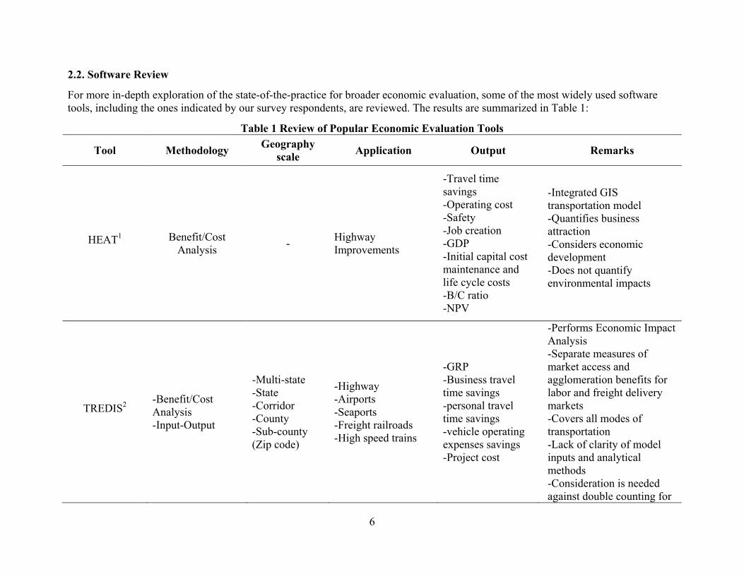
2.2. Software Review
For more in-depth exploration of the state-of-the-practice for broader economic evaluation, some of the most widely used software tools, including the ones indicated by our survey respondents, are reviewed. The results are summarized in Table 1:
Table 1 Review of Popular Economic Evaluation Tools
Tool Methodology Geography
scale Application Output Remarks
HEAT1 Benefit/Cost Analysis
- Highway Improvements
-Travel time savings -Operating cost -Safety -Job creation -GDP -Initial capital cost maintenance and life cycle costs -B/C ratio -NPV
-Integrated GIS transportation model -Quantifies business attraction -Considers economic development -Does not quantify environmental impacts
TREDIS2 -Benefit/Cost Analysis -Input-Output
-Multi-state -State -Corridor -County -Sub-county (Zip code)
-Highway -Airports -Seaports -Freight railroads -High speed trains
-GRP -Business travel time savings -personal travel time savings -vehicle operating expenses savings -Project cost
-Performs Economic Impact Analysis -Separate measures of market access and agglomeration benefits for labor and freight delivery markets -Covers all modes of transportation -Lack of clarity of model inputs and analytical methods -Consideration is needed against double counting for
7
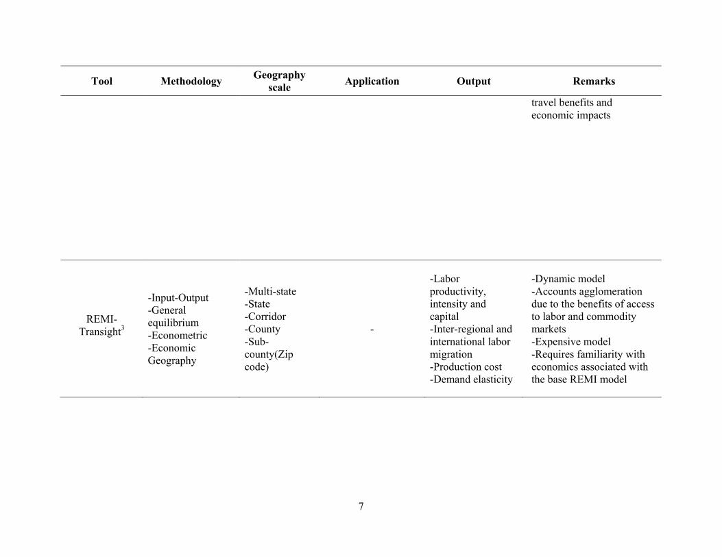
Tool Methodology Geography
scale Application Output Remarks
travel benefits and economic impacts
REMI-Transight3
-Input-Output -General equilibrium -Econometric -Economic Geography
-Multi-state -State -Corridor -County -Sub-county(Zip code)
-
-Labor productivity, intensity and capital -Inter-regional and international labor migration -Production cost -Demand elasticity
-Dynamic model -Accounts agglomeration due to the benefits of access to labor and commodity markets -Expensive model -Requires familiarity with economics associated with the base REMI model

8
Tool Methodology Geography
scale Application Output Remarks
IMPLAN4 Input-Output
-Multi-state -State -Corridor -County -Sub-county (Zip code)
Impact of: -New businesses -Tourism -Agriculture -Resource management -Higher Education
-Economic value of project -Job creation -Value added: total payroll costs, income, payments for rents, property taxes, fees
-software interface easy to use -Application of economic geography -Can be supplemented by other tools like TREDIS or REMI-Transight -Does not have any of the transportation demand parameters -It is not dynamic
MicroBENCOST5 Benefit/Cost
Analysis Corridor
Highway Improvements
-NPV -Gross B/C ratio -Net B/C ratio -Internal rate of return
-Some default data cannot be changed -Some data could be out of date -Does not quantify environmental impacts
STEAM6 Benefit/Cost Analysis
Corridor or regional level
-Multi-modal urban infrastructure investments
-NPV -B/C ratio
-Performs Risk Analysis -Not a dynamic model -Some default inputs cannot be changed
StratBENCOST7 Benefit/Cost
Analysis -
Highway Improvements
-B/C ratio -Internal rate of return -NPV -Total benefit -Total cost
Performs Risk Analysis

9
Tool Methodology Geography
scale Application Output Remarks
MPPP8 Benefit/Cost Analysis
- Highway Improvements
-B/C ratio -Travel time savings & distribution -NPV -Daily user benefit -Present value of user benefits
-Methodology is clear to users -Does not include economic productivity and economic impact in broader level -Some data may be out of date -Does not account for truck freight benefits separately for highway projects
BCA.Net9 Benefit/Cost Analysis
- Highway projects
-Net Present Value -Benefit-Cost ratio -Internal rate of return
-Default inputs can be modified -User friendly -Performs Risk Analysis
Cal-B/C10 Benefit/Cost Analysis
-
-Highway Improvements -Transit projects -Intelligent Transportation System(ITS) -Transportation Management System(TMS) -Operational Improvements
-Life-Cycle costs -Life-Cycle benefits -NPV -Benefit-Cost Ratio -Rate of return on investment -Project payback period
-Revised several times to cover TMS, ITS and operational improvements -Provides Technical Supplement to User’s Guide explaining the methodology in detail
HERS-ST11 Benefit/Cost Analysis
- Highway Improvements
-System conditions: total vehicle miles of travel, total cost of improvements, simulated pavement conditions, total
-Case of new highway segment or improving non-highway modes are not considered within the tool -Performs sensitivity analysis
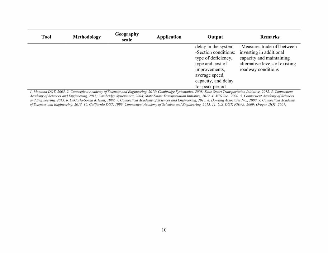
10
Tool Methodology Geography
scale Application Output Remarks
delay in the system -Section conditions: type of deficiency, type and cost of improvements, average speed, capacity, and delay for peak period
-Measures trade-off between investing in additional capacity and maintaining alternative levels of existing roadway conditions
1. Montana DOT, 2005. 2. Connecticut Academy of Sciences and Engineering, 2013; Cambridge Systematics, 2008; State Smart Transportation Initiative, 2012. 3. Connecticut Academy of Sciences and Engineering, 2013; Cambridge Systematics, 2008; State Smart Transportation Initiative, 2012. 4. MIG Inc., 2000. 5. Connecticut Academy of Sciences and Engineering, 2013. 6. DeCorla-Souza & Hunt, 1999, 7. Connecticut Academy of Sciences and Engineering, 2013. 8. Dowling Associates Inc., 2000. 9. Connecticut Academy of Sciences and Engineering, 2013. 10. California DOT, 1999; Connecticut Academy of Sciences and Engineering, 2013. 11. U.S. DOT, FHWA, 2009; Oregon DOT, 2007.

11
3. METHODOLOGY AND TOOLS OVERVIEW
This research’s most important contribution is to show how states can benefit from incorporating SHRP2 C11 tools into their current practices. The authors demonstrated the integration of SHRP2 C11 tools with the Maryland Statewide Transportation Model (MSTM) with case studies. In the following sections, the functionality and the main attributes of each tool are discussed and the seven-level integration framework is provided and reviewed.
3.1.Maryland Statewide Transportation Model (MSTM)
The MSTM is the statewide four-step travel demand model currently used by the Maryland State Highway Administration (SHA) that allows consistent estimates of future development impacts on transportation performance measures. MSTM is a multi-layer model applicable at the regional, statewide or urban level, providing analytical support in SHA’s current decision-making process regarding the implementation of transportation policies and the prioritization of projects throughout the State of Maryland (Maryland State Highway Administration, 2013). The MSTM results were obtained using the default study area, which consists of Maryland, Delaware, Washington, D.C., and parts of New Jersey, Pennsylvania, Virginia and West Virginia; therefore, it is reasonable to perform the SHRP2 C11 analysis assuming an impact area consisting of Maryland, Virginia and Washington, D.C. An overall view of the MSTM model components is provided in Figure 1.
Figure 1 MSTM Model Components (Maryland State Highway Administration, 2013).

12
3.2.SHRP2 Capacity Project C11: Development of Tools for Assessing Broader Economic Benefits of Transportation
This section provides a brief introduction of the main attributes of the four SHRP2 C11 tools that are applicable to the case studies: (i) the Buyer-Supplier Market Access tool, (ii) the Intermodal Connectivity tool, (iii) the Reliability tool and (iv) the Accounting Framework tool. These tools can be used at the policy and funding stage, the planning/strategy stage, the capital programming stage, the project prioritization stage, and the project development stage, to facilitate or support decision-making. For more detailed information on the tools, readers may refer to the SHRP2 C11 Users’ Guide (National Academy of Science, 2013).
The Buyer-Supplier Market Access Tool uses information on zonal activity, such as population and employment, generalized cost and Gross Regional Product (GRP) before and after the investment, to estimate truck accessibility from firms to buyers and suppliers. The estimated metrics include effective density (as a measure of accessibility to employment), potential access, regional labor pool, and total productivity. The tool can be used to estimate the changes in market access that can be attributed to a new transportation project.
The Reliability Tool uses information on the facility, traffic, capacity, value of travel time, incidents and reliability. The output includes metrics such as incident delay, total delay, cost of recurring delay, and cost of unreliability. Like the Market Access tool, the Reliability tool can be run for a no-build and build scenario, estimating the travel time reliability improvement in the study area that can be attributed to a new transportation project.
The Intermodal Connectivity Tool assesses changes in connectivity for an intermodal facility following a highway improvement in the facility’s vicinity. Information regarding the highway improvement, such as volume, access time and the fraction of freight vehicles affected by the highway improvement, is required as input. Information on existing intermodal facilities in the U.S. is readily available within the Intermodal Connectivity Tool spreadsheet. The output of this tool is the weighted connectivity index of the facility with respect to the particular highway improvement. The tool’s main functionality is to compare different highway improvements with respect to how much each improvement enhances the facility’s connectivity.
The Accounting Framework Tool assigns a dollar value to the broader benefits estimated by the previous SHRP2 C11 tools and it also estimates the traditional direct project benefits related to vehicle operating cost, travel time and safety. Both direct and broader benefits are based upon assumed values for vehicle occupancy, vehicle operating cost per mile, value of time, value of reliability, average cost per crash and productivity elasticity.
Typically, the SHRP2 C11 tools are used for corridor-level analysis and do not account for the network effects in the broader region surrounding the investment location. A recent report (NCHRP, 2014) showcases how the SHRP2 C11 tools were used for three different case studies. In all three cases, the analysis was performed at a restricted, corridor-level scale, without capturing the benefits of a full-scale travel demand model, as the proposed seven-level integrated framework does. Therefore, the research conducted as part of this project adds to the state-of-the art in multiple levels. First, the research team analyzed the economic benefits of new transportation infrastructure investment by integrating an economic analysis tool with a statewide travel demand model. This integration is useful to policymakers at the state level, as this paper describes how to easily and effectively incorporate the open-source SHRP2 tools with

13
the travel demand model that most states already have in place. Second, the authors enhanced the SHRP2 tools by showing how proper customization of the default parameters can yield sound results for Maryland. This customization will encourage policymakers and other stakeholders to customize the tools for their own state and use them to guide and support project selection and prioritization.
3.3.Travel Demand Model & Economic Analysis Tool Integration Framework
Following the description of the main characteristics of MSTM and the selected SHRP2 C11 tools applicable to the case studies, this section describes the process of integrating these tools into MSTM. The description of the process, further illustrated in Figure 2, shows the convenience of using the SHRP2 C11 tools as an economic analysis tool along with MSTM, especially considering the compatibility and the interoperability of the two tools in terms of data inputs and outputs.
Level 1: The first level in this integrated process runs MSTM for all scenarios selected for evaluation. These scenarios include years 2007 and 2030, under the no-build and build assumption for the project. For each different scenario, input data include the highway and transit network, as well as socioeconomic, household, employment and land-use information.
Level 2: This level includes all corridor-specific data obtained from MSTM for each scenario to be used as inputs in the SHRP2 tools. This information includes: (i) infrastructure-specific information such as functional class, length, and number of lanes, (ii) traffic data, such as Annual Average Daily Traffic (AADT), truck percentage and free flow speed, (iii) capacity data, and (iv) impedance data, in terms of generalized cost for all origin-destination (OD) pairs in the study area.
Level 3: In the third level of the integration process, activity-related data regarding employment and population, as well as economic data in terms of GRP per capita are collected from external sources for each scenario.
Level 4: The fourth level is the most critical step in the integration process. Selected MSTM and other data are used as inputs in the SHRP2 C11 tools following proper data processing to achieve compatibility between the two tools. Infrastructure data, traffic data and capacity data obtained from MSTM are used as inputs in the SHRP2 Reliability tool; the Market Access Tool uses data on impedance data, activity data and GRP data; the Intermodal Connectivity Tool uses traffic data (such as truck volume and access time). The related metrics are generated in the next level.
Level 5: Among other metrics, the Reliability tool assesses the impact of new investment on incident-related delays and the cost of unreliability, the Market Access tool captures changes in market accessibility as a result of the new project, and the Intermodal Connectivity tool estimates the weighted connectivity index for each facility that is evaluated.
Level 6: The metrics generated in Level 5 serve as inputs in the Accounting Framework Tool, which assigns a monetary value to the estimated benefits. The value reflects savings from reduced non-recurring delay, GRP gains due to increased effective market size, and monetary benefits due to increased intermodal connectivity. In this level, assumptions are made about the GRP elasticity with respect to effective density, value of time and reliability ratio.
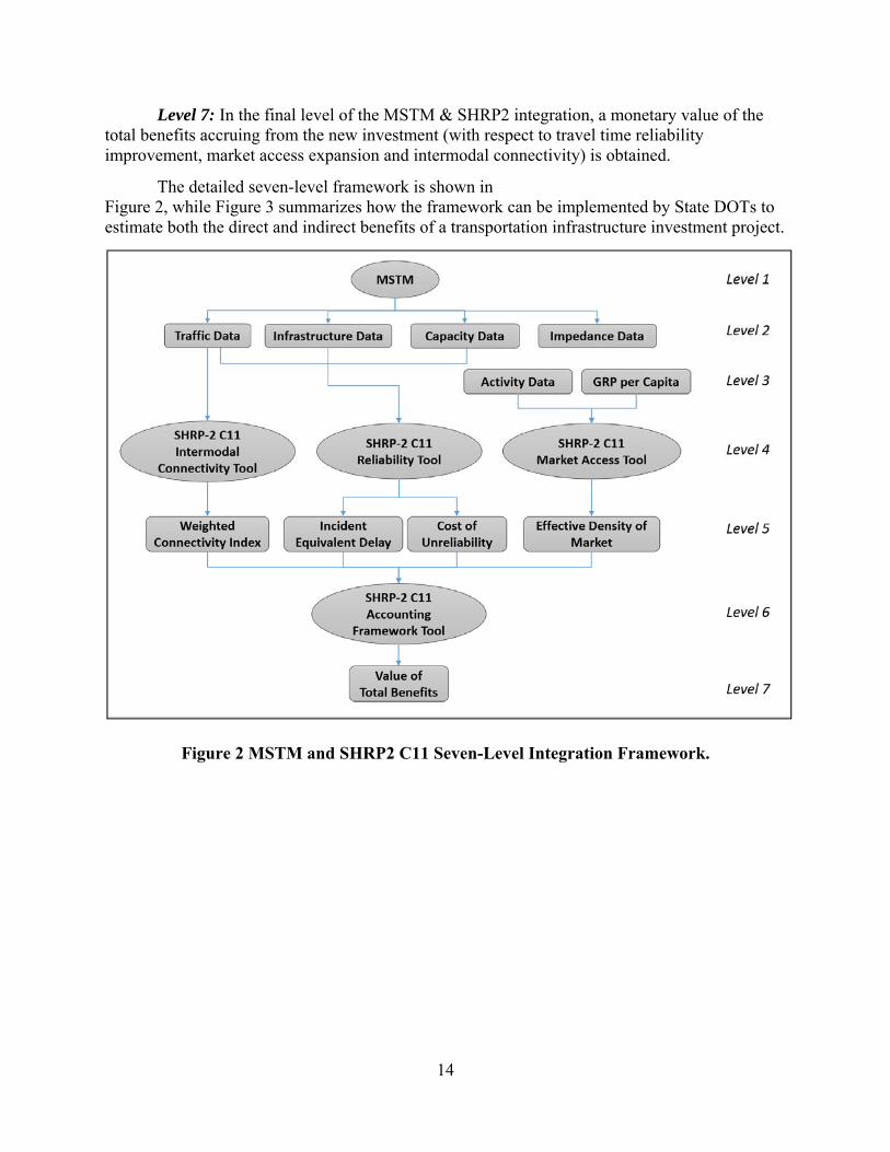
14
Level 7: In the final level of the MSTM & SHRP2 integration, a monetary value of the total benefits accruing from the new investment (with respect to travel time reliability improvement, market access expansion and intermodal connectivity) is obtained.
The detailed seven-level framework is shown in Figure 2, while Figure 3 summarizes how the framework can be implemented by State DOTs to estimate both the direct and indirect benefits of a transportation infrastructure investment project.
Figure 2 MSTM and SHRP2 C11 Seven-Level Integration Framework.

15
Figure 3 Integrated Framework Implementation at the State DOT level
4. DATA INTEGRATION
The main advantage of integrating the SHRP2 C11 products with an existing travel demand model is the interoperability of the two tools with regard to input and output data. This section describes the process of obtaining, post-processing and re-using the data.
Market access benefits are estimated for the year 2030, between the no-build scenario where the new investment is not included in the transportation network and the build scenario. The MSTM results were processed and aggregated at the county level, providing demand tables and skim matrices for the two scenarios. Using a value of time of 23.3 cents per minute based on MSTM, the skim matrix presents the generalized cost in dollars per trip, for trips between all OD pairs in the study area, based on Equation (1):
Generalized cost = Toll + Value of time + travel time (1)
In addition to the MSTM data, some activity and economic data are also required for the integration to be successful. For this case study, population, employment and GRP per capita data from 1980 to 2008 at the county level for the entire United States were collected from a commercial database called the Complete Economic and Demographic Data Source (CEDDS), provided by Woods and Poole Economics.
5. PARAMETER CUSTOMIZATION FOR MARYLAND
Changes in transportation systems can reduce search costs and facilitate the sourcing decisions for business sectors, improving the buyer-supplier and labor accessibility. System changes can also affect the location choices of firms and households and overall land use activities that may influence accessibility to markets and labor pools (Zondag et al., 2014).

16
Consequently, improved market accessibility reduces the cost of obtaining raw materials, accessing the labor pool and supplying finished products to consumers (Chandra and Vadali, 2014). Additionally, Targa et al. (2005) found a positive relationship between roadway accessibility and business density in the zip code area. Improved travel time reliability increases consumer benefits, allows manufacturers to minimize their inventory costs and helps them schedule assembly and distribution logistics, thus enhancing the business environment and boosting the region’s economy (Kato et al., 2014).
Using the information presented earlier, this section presents the parameter customization process for the State of Maryland. In addition to integrating MSTM with SHRP2, customizing the SHRP2 C11 default parameters is an important contribution of this research project, leading to sound estimation results that planners, engineers and policymakers at the state DOT can trust and use in their decision-making process. It also helps states tailor the SHRP2 C11 tools to the economic, demographic and travel conditions in their region.
The SHRP2 parameters available for tuning are:
Impedance Decay Parameter α (Buyer-Supplier Market Access Tool): the impedance decay parameter is a behavioral parameter and it can go as high as 5 or 6. Based on the Model of Sustainability and Integrated Corridors (MOSAIC) for comprehensive highway corridor planning developed previously by Zhang et al. (2013), the value of α was set as 1. A decay factor of 1 captures the observed spatial distribution of trips in Maryland and the effect of the Inter-County Connector (ICC) on counties located further away from the investment location. Also, as suggested in the SHRP2 C11 User’s Guide, a sensitivity analysis was performed for alpha, with values ranging from 1 to 4, to understand how alpha affects the estimation results. Indeed, for alpha = 1, there is confidence that the market access benefits are not overestimated, since the access benefits increase as α increases.
Value of Time (VOT) (Reliability Tool): Default values of $19.86 and $36.05 per hour are assumed for personal and commercial trips, respectively in SHRP2 C11. To customize the tool for Maryland and to further integrate SHRP2 C11 with MSTM, the authors use the MSTM-specific VOT: 14 and 63.8 $ per hour (23.3 and 106.4 cents per minute) for personal and commercial travel, respectively.
Reliability Ratio RR (Reliability Tool): Default values of 0.8 and 1.16 are assumed for personal and commercial trips, respectively, and the User’s Guide provides a review of the reliability ratio values used in various studies. Currently, SHA uses a reliability ratio of 0.75 for congestion-relief projects without differentiating between personal and commercial trips.
Productivity elasticity with respect to market access μ (Buyer-Supplier Market Access Tool): there is a range of recommended values provided in the User’s Guide for different types of investment and activity data, from less than 0.03 for improvement projects, to 0.06 for new capacity, when population activity data is used. Using Maryland-specific econometric models developed to estimate the productivity elasticity with respect to employment, the authors select μ = 0.01 (He et al., 2014) for all types of activities in this study. The econometric models developed in He et al. (He et al., 2014) include all industry sectors in Maryland, as there is no strong evidence that some industrial sectors in Maryland have larger shares of the economy than others (He et al., 2015).

17
6. CASE STUDIES
Four case studies were selected to demonstrate how the integrated framework works for different types of projects. The locations of the four case studies are shown in Figure 4, while the next subsections discuss the details of each project and present the estimation results.
Figure 4 Comprehensive Map of the 5 Conducted Case Studies
6.1.INTERCOUNTY CONNECTOR (ICC)
I. Project Description
The ICC, MD 200, is a new tolled freeway in Maryland that connects Gaithersburg in Montgomery County and Laurel in Prince George's County. It covers approximately 18.8 miles and includes highway interchanges and bridges that provide multiple benefits to the Washington and Baltimore metropolitan areas, such as increasing the mobility and reliability of trips,

18
accommodating passenger and goods movements, and increasing community safety (Heyer and McClure, 2011; Bodin et al., 2004). Table 2 presents the main case study characteristics, while Figure 5 depicts the case study and the corresponding study area.
Table 2 ICC Case Study Characteristics Case Study Improvement
Type # of Lanes/ Direction
Length (mi) Study Region
Cost ($)
ICC New
Construction 3 18.8 2 counties* 2,560M**
* Montgomery, Prince George’s ** Adapted from FHWA website: http://www.fhwa.dot.gov/ipd/project_profiles/md_icc.aspx
Figure 5 Inter-County Connector Case Study and Study Area
Three parallel routes (Randolph Road, Bel Pre Road and MD 28/MD 198) that initially served the east-west traffic flow in the study area were selected to evaluate the effect of ICC on their mobility attributes. In particular, it is assumed that, upon construction of ICC, traffic diverts from these three corridors towards ICC, leading to lower congestion levels, improved accessibility and higher travel time reliability along these parallel routes (Pu et al., 2013). The selection of the three routes is consistent with past research from Maryland State Highway Administration (SHA) (Pu et al., 2013). It is assumed that ICC does not significantly affect the I-495 traffic patterns, since I-495 primarily serves traffic between Maryland and Virginia, whereas the ICC, MD 28/MD 198, Bel Pre Road and Randolph Road mainly serve intrastate east-west traffic.

19
II. Direct Benefits Estimation
To compare the order of magnitude between direct and broader benefits, the authors also estimated the standard direct benefits for 2030, including travel time cost savings and vehicle operation cost savings based on travel time, distance, speed and vehicle-miles-traveled. The economic value of travel time savings is estimated by multiplying the change in travel time by the value of time (14 $/hour for automobiles and 63.8 $/hour for trucks). The fuel cost savings is estimated using fuel consumption as a function of average operation speed and with the assumption that the gas price is $1.314 per gallon (Bodin et al., 2004). It should be noted that the gas price is derived from MSTM default parameters, which is lower than the real gas price (approximately $2.00 per gallon). More accurate results can be achieved by using a higher value for gas price, but this study uses the aforementioned value to be consistent with MSTM settings. Furthermore, values of $0.04 and $0.05 per mile for auto and truck, respectively, are used to estimate maintenance and tire costs (Bodin et al., 2004). Both the direct and broader benefits are estimated based on MSTM default parametersin year 2000 dollar and then adjusted to year 2015 dollar, using the latest Consumer Price Index (CPI) provided by the Bureau of Labor Statistics (2015) to account for inflation. It should be noted that the same methodology is used for the other case studies to assess the direct benefits. Table 3 presents the value of direct benefits for the ICC case study.
Table 3 Annual Direct Benefits for ICC Case Study Source of Benefit Value of Total Benefit ($) Travel Time $49.75 million Fuel Cost $2.66 million Maintenance Cost $0.89 million Total Direct Benefits $53.3 million

20
III. Broader Benefits Estimation
Market Accessibility Benefits
Based on the integration framework illustrated in Figure 2 and the Maryland-specific customized values of the SHRP2 C11 parameters, the market access and travel-time reliability benefits are estimated. Table 4 presents the changes in effective density1 that can be attributed to the ICC construction for each of the 13 counties in the study area in the year 2030. The effective density of each county is calculated for the 2030 no-build and 2030 build scenarios, using population and GRP data for each county, as well as using impedance data for all county pairs.
The estimation results from the Buyer-Supplier tool show that by the year 2030, the effective density and the corresponding productivity of both counties in the study area will increase, while the overall market accessibility improves by an average of 0.6 percent after ICC is incorporated in the network.
Table 4 Buyer-Supplier Market Access Tool Results County % Δ(Effective Density)
Montgomery, MD 0.8%
Prince George’s, MD 0.5%
Total 1.3%
1 The effective density of employment or population accessible to any firm in industry o located in zone i is:
where : the employment or population in zone i , : the total employment or population in zone j, :
the impedance between i and j, and : the impedance decay parameter. The scale factor is defined as follows:
where : the employment or population of the zone for which the effective density is calculated, : the
area of the zone for which effective density is calculated, and : the impedance decay parameter.

21
Travel Time Reliability Benefits
Evaluation of the improved travel time reliability is performed for the year 2030, for the three routes where congestion will be significantly alleviated by ICC. The summary results for the three parallel routes are presented in Table 5. It should be noted that the analysis presented here refers to the reliability improvements along the three parallel routes only, and does not capture the overall changes in reliability for the entire network. For reliability improvements occurring in the entire network, the authors would have to account for the vehicles diverted to the newly constructed facility, which will most probably experience some travel delay.
The results show that all three corridors will experience a travel time reliability improvement attributable to ICC. Specifically, Randolph Road will experience a reduction of 34 percent and 50 percent in recurring and incident-related delays, respectively; MD 28/MD 198 will also experience similar levels of improvement. This large improvement along Bel Pre Road is due to the fact that in the 2030 no-build scenario Bel Pre Road does not experience any congestion. Once included in the network, ICC further improves the already good travel conditions along Bel Pre Rd. These results suggests that the Travel Time Reliability tool is better suited to model roadway segments that experience some level of congestion in the no-build scenario.
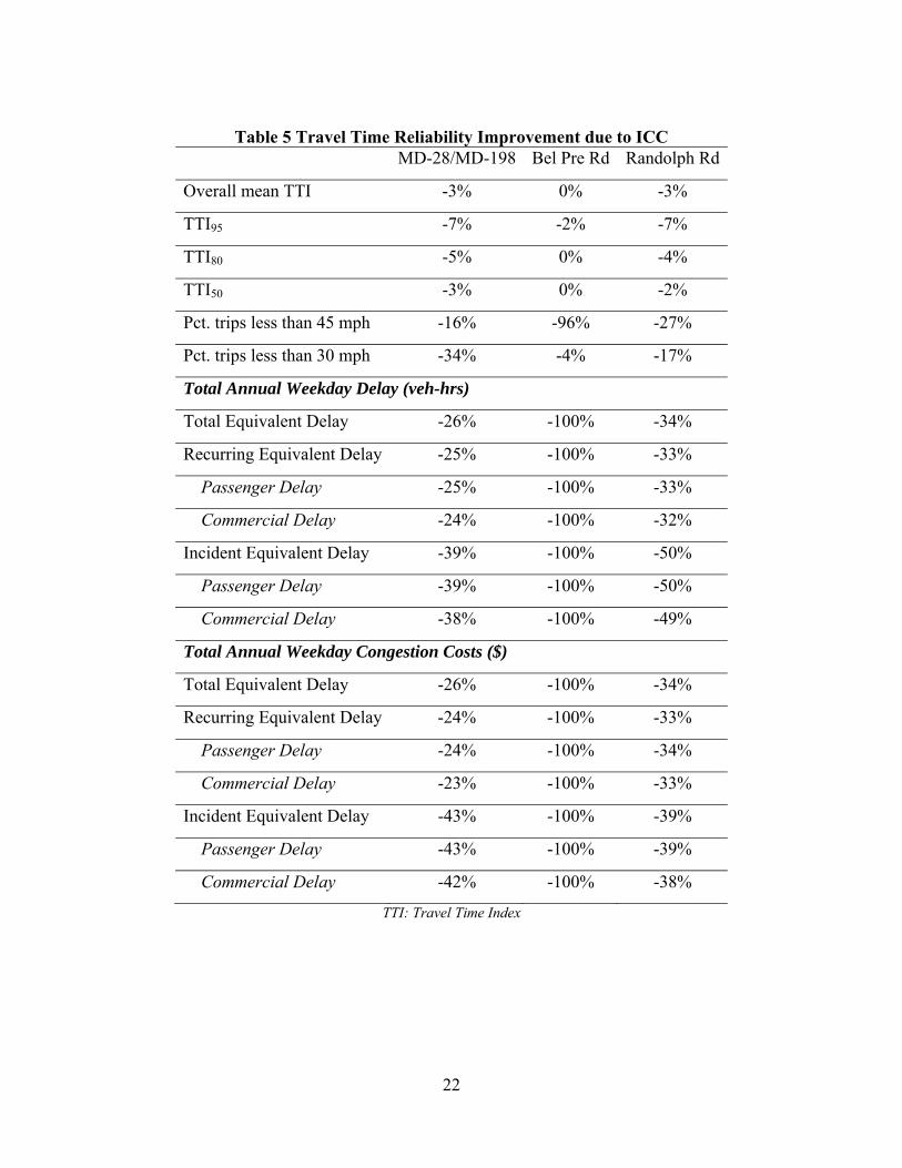
22
Table 5 Travel Time Reliability Improvement due to ICC MD-28/MD-198 Bel Pre Rd Randolph Rd
Overall mean TTI -3% 0% -3%
TTI95 -7% -2% -7%
TTI80 -5% 0% -4%
TTI50 -3% 0% -2%
Pct. trips less than 45 mph -16% -96% -27%
Pct. trips less than 30 mph -34% -4% -17%
Total Annual Weekday Delay (veh-hrs)
Total Equivalent Delay -26% -100% -34%
Recurring Equivalent Delay -25% -100% -33%
Passenger Delay -25% -100% -33%
Commercial Delay -24% -100% -32%
Incident Equivalent Delay -39% -100% -50%
Passenger Delay -39% -100% -50%
Commercial Delay -38% -100% -49%
Total Annual Weekday Congestion Costs ($)
Total Equivalent Delay -26% -100% -34%
Recurring Equivalent Delay -24% -100% -33%
Passenger Delay -24% -100% -34%
Commercial Delay -23% -100% -33%
Incident Equivalent Delay -43% -100% -39%
Passenger Delay -43% -100% -39%
Commercial Delay -42% -100% -38%
TTI: Travel Time Index
23
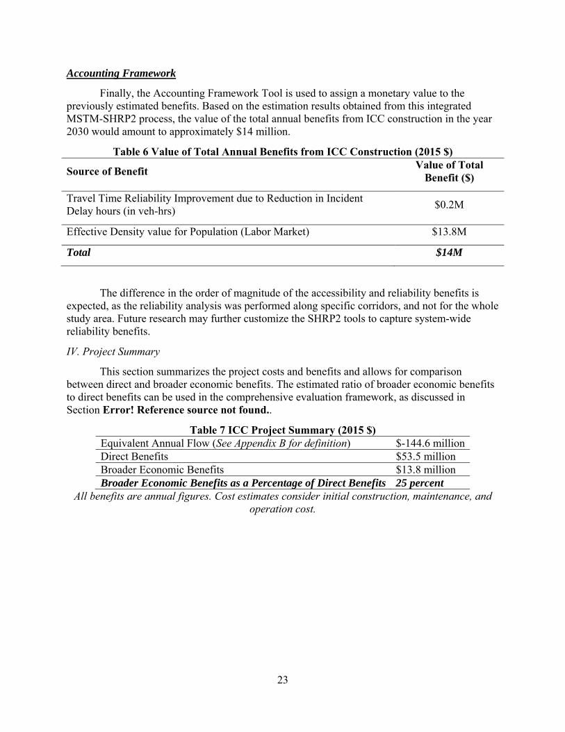
Accounting Framework
Finally, the Accounting Framework Tool is used to assign a monetary value to the previously estimated benefits. Based on the estimation results obtained from this integrated MSTM-SHRP2 process, the value of the total annual benefits from ICC construction in the year 2030 would amount to approximately $14 million.
Table 6 Value of Total Annual Benefits from ICC Construction (2015 $)
Source of Benefit Value of Total
Benefit ($)
Travel Time Reliability Improvement due to Reduction in Incident Delay hours (in veh-hrs)
$0.2M
Effective Density value for Population (Labor Market) $13.8M
Total $14M
The difference in the order of magnitude of the accessibility and reliability benefits is expected, as the reliability analysis was performed along specific corridors, and not for the whole study area. Future research may further customize the SHRP2 tools to capture system-wide reliability benefits.
IV. Project Summary
This section summarizes the project costs and benefits and allows for comparison between direct and broader economic benefits. The estimated ratio of broader economic benefits to direct benefits can be used in the comprehensive evaluation framework, as discussed in Section Error! Reference source not found..
Table 7 ICC Project Summary (2015 $) Equivalent Annual Flow (See Appendix B for definition) $-144.6 millionDirect Benefits $53.5 million Broader Economic Benefits $13.8 million Broader Economic Benefits as a Percentage of Direct Benefits 25 percent
All benefits are annual figures. Cost estimates consider initial construction, maintenance, and operation cost.

24
6.2.EXPRESS TOLL LANES
I. Project Description
Express toll lanes (ETL) are new tolled travel lanes separated by a concrete barrier from general-purpose lanes. Toll rates vary by time of day based on traffic conditions.
The Baltimore ETL project is part of the $1.08 billion I-95 Improvement Project, which includes $756 million in highway and safety improvements along the 8 miles of I-95 from the I-895 interchange to north of White Marsh Boulevard (MD 43) in northeast Baltimore(Figure 6). Table 8 presents the ETL case study characteristics
Figure 6 Express Toll Lanes Case Study and Study Area
25
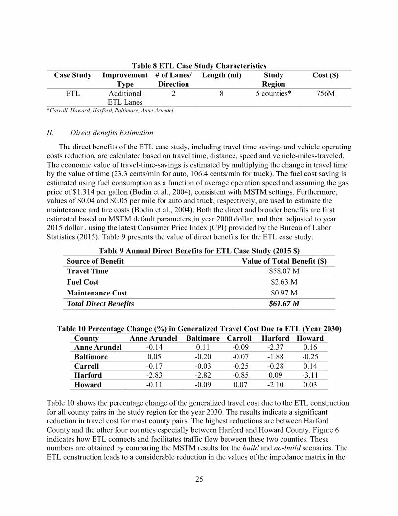
Table 8 ETL Case Study Characteristics Case Study Improvement
Type # of Lanes/ Direction
Length (mi) Study Region
Cost ($)
ETL Additional ETL Lanes
2 8 5 counties* 756M
*Carroll, Howard, Harford, Baltimore, Anne Arundel
II. Direct Benefits Estimation
The direct benefits of the ETL case study, including travel time savings and vehicle operating costs reduction, are calculated based on travel time, distance, speed and vehicle-miles-traveled. The economic value of travel-time-savings is estimated by multiplying the change in travel time by the value of time (23.3 cents/min for auto, 106.4 cents/min for truck). The fuel cost saving is estimated using fuel consumption as a function of average operation speed and assuming the gas price of $1.314 per gallon (Bodin et al., 2004), consistent with MSTM settings. Furthermore, values of $0.04 and $0.05 per mile for auto and truck, respectively, are used to estimate the maintenance and tire costs (Bodin et al., 2004). Both the direct and broader benefits are first estimated based on MSTM default parameters,in year 2000 dollar, and then adjusted to year 2015 dollar , using the latest Consumer Price Index (CPI) provided by the Bureau of Labor Statistics (2015). Table 9 presents the value of direct benefits for the ETL case study.
Table 9 Annual Direct Benefits for ETL Case Study (2015 $) Source of Benefit Value of Total Benefit ($) Travel Time $58.07 M
Fuel Cost $2.63 M
Maintenance Cost $0.97 M
Total Direct Benefits $61.67 M
Table 10 Percentage Change (%) in Generalized Travel Cost Due to ETL (Year 2030) County Anne Arundel Baltimore Carroll Harford Howard Anne Arundel -0.14 0.11 -0.09 -2.37 0.16 Baltimore 0.05 -0.20 -0.07 -1.88 -0.25 Carroll -0.17 -0.03 -0.25 -0.28 0.14 Harford -2.83 -2.82 -0.85 0.09 -3.11 Howard -0.11 -0.09 0.07 -2.10 0.03
Table 10 shows the percentage change of the generalized travel cost due to the ETL construction for all county pairs in the study region for the year 2030. The results indicate a significant reduction in travel cost for most county pairs. The highest reductions are between Harford County and the other four counties especially between Harford and Howard County. Figure 6 indicates how ETL connects and facilitates traffic flow between these two counties. These numbers are obtained by comparing the MSTM results for the build and no-build scenarios. The ETL construction leads to a considerable reduction in the values of the impedance matrix in the

26
study area, as it provides additional capacity in the system by mitigating congestion on general purpose lanes, reducing travel time and ultimately reducing the generalized travel cost along the links.
III. Broader Benefits Estimation
Market Accessibility Benefits
Based on the integration framework illustrated in Figure 2 and the Maryland-specific customized values of the SHRP2 parameters, the market access and travel-time reliability benefits are estimated. Table 11 presents the changes in effective density that can be attributed to the ETL construction for each one of the five counties of the study area in the year 2030. The effective density of each county is calculated for the 2030 no-build and 2030 build scenarios, using population and GRP data for each county, as well as impedance data for all county pairs.
The estimation results from the Buyer-Supplier tool show that, by the year 2030, the effective density and the corresponding productivity of all five counties in the study area will increase, while Harford County will experience the largest increase in effective density, compared to the no-build scenario. The overall market accessibility improves after the ETL are incorporated in the network by an average of 0.4 percent.
Table 11 Buyer-Supplier Market Access Tool Results County % Δ(Effective Density)Anne Arundel 0.1% Baltimore 0.3% Carroll 0.1% Harford 1.6% Howard 0.1% Total 0.4%
Travel-Time Reliability Benefits
Evaluation of the improved travel time reliability is performed for the year 2030. The summary results for the no-build and build scenarios are presented in

27
Table 12. It should be noted that the analysis presented here refers to the reliability improvements along the general-purpose lanes only and does not capture overall changes in reliability for the entire network.
The results show that the general-purpose lanes will experience a travel time reliability improvement that can be attributed to the ETL construction.
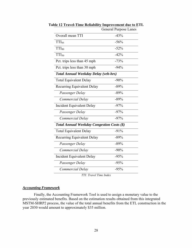
28
Table 12 Travel-Time Reliability Improvement due to ETL General Purpose Lanes
Overall mean TTI -43%
TTI95 -56%
TTI80 -52%
TTI50 -42%
Pct. trips less than 45 mph -73%
Pct. trips less than 30 mph -94%
Total Annual Weekday Delay (veh-hrs)
Total Equivalent Delay -90%
Recurring Equivalent Delay -89%
Passenger Delay -89%
Commercial Delay -89%
Incident Equivalent Delay -97%
Passenger Delay -97%
Commercial Delay -97%
Total Annual Weekday Congestion Costs ($)
Total Equivalent Delay -91%
Recurring Equivalent Delay -89%
Passenger Delay -89%
Commercial Delay -90%
Incident Equivalent Delay -95%
Passenger Delay -95%
Commercial Delay -95%
TTI: Travel Time Index
Accounting Framework
Finally, the Accounting Framework Tool is used to assign a monetary value to the previously estimated benefits. Based on the estimation results obtained from this integrated MSTM-SHRP2 process, the value of the total annual benefits from the ETL construction in the year 2030 would amount to approximately $35 million.

29
Table 13 Value of Total Annual Benefits (2015 $)
Source of Benefit Value of Total
Benefit ($)
Travel-Time-Reliability Improvement due to Reduction in Incident Delay hours (in veh-hrs) $27.4M
Effective Density value for Population (Labor Market) $7.6M
Total $35M
IV. Project Summary
This section summarizes the project costs and benefits and allows for comparison between the level of magnitude between direct and broader economic benefits. The estimated ratio of broader economic benefits to direct benefits can be used as part of the proposed streamlined ratio approach of the comprehensive evaluation framework, as discussed in Section Error! Reference source not found..
Table 14 Express Toll Lanes Project Summary (2015 $) Equivalent Annual Flow (See Appendix B for definition) $26.4M Direct Benefits $89.07M Broader Economic Benefits $7.6M Broader Economic Benefits as a Percentage of Direct Benefits 8.5%
All benefits are annual figures. Cost estimates consider initial construction, maintenance and operation cost.
6.3.LOCAL CONNECTOR
I. Project Description
The new road link between Viers Mill Road and Randolph Road in Montgomery County is expected to provide better connectivity and relieve congestion over the connecting roads. The project includes adding two lanes in each direction and extending the centerline for 1.25 miles. Figure 7 and Table 15 present the main case study characteristics.
Table 15 Local Connector Case Study Characteristics Case Study Improvement
Type # of Lanes/ Direction
Length (mi) Study Region
Cost ($)
Local Connector
New Construction
2 1.25 7 TAZs in Montgomery
County
75M

30
Figure 7 Local Connector Case Study and Study Area
II. Direct Benefits Estimation
The direct benefits for the local connector case study, including travel-time savings and vehicle operating costs, are calculated based on travel time, distance, speed and vehicle-miles-traveled. The economic value of travel-time savings is estimated by multiplying the change in travel time by the value of time (23.3 cents/min for auto, 106.4 cents/min for truck). The fuel cost saving is estimated using fuel consumption as a function of average operation speed and assuming $1.314 per gallon is the gas price (Bodin et al., 2004), consistent with MSTM settings. Furthermore, values of $0.04 and $0.05 per mile for auto and truck, respectively, are used as the maintenance and tire costs (Bodin et al., 2004). Both the direct and broader benefits are estimated based on MSTM default parametersin year 2000 dollar and then adjusted to year 2015 dollar, using the latest Consumer Price Index (CPI) provided by the Bureau of Labor Statistics (2015).

31
Table 16 presents the value of direct benefits for the local connector case study.

32
Table 16 Annual Direct Benefits for the Local Connector Case Study (2015 $) Source of Benefit Value of Total Benefit ($)Travel Time $8.73 million
Fuel Cost insignificant
Maintenance Cost insignificant
Total Direct Benefits $8.73 million
III. Broader Benefits Estimation
Market Accessibility Benefits
Based on the integration framework illustrated in Figure 2 and the Maryland-specific SHRP2 C11 parameters, the market access and travel-time reliability benefits are estimated. Table 17 presents the changes in effective density that can be attributed to the new local connector for each one of the three Traffic Analysis Zones (TAZs) of the study area in the year 2030. The effective density of each county is calculated for the 2030 no-build and 2030 build scenarios, using population and GRP data for each county, as well as impedance data for all county pairs.
The estimation results from the Buyer-Supplier tool show that by the year 2030, the effective density and the corresponding productivity of all three zones in the study area will increase, compared to the no-build scenario. The overall market accessibility improves after the new local connector is introduced in the network by an average of 9 percent.
Table 17 Buyer-Supplier Market Access Tool Results Zone % Δ(Effective Density)
654 10%
659 9%
698 9%
Total 9%
Travel-Time Reliability Benefits
The Travel-Time Reliability Tool was used to quantify the travel-time reliability benefits accrued from the addition of the local connector. However, the results are not statistically significant and thus are not presented here.
Accounting Framework
Finally, the Accounting Framework Tool is used to assign a monetary value to the estimated benefits. The value of the total annual benefits from the new local connector in the year 2030 would amount to approximately $1.5 million.

33
Table 18 Value of Total Annual Benefits (2015 $)
Source of Benefit Value of Total
Benefit ($)
Travel Time Reliability Improvement due to Reduction in Incident Delay hours (in veh-hrs)
insignificant
Effective Density value for Population (Labor Market) $1.5M
Total $1.5M
IV. Project Summary
This section summarizes the project costs and benefits and allows for comparison between the level of magnitude between direct and broader economic benefits. The estimated ratio of broader economic benefits to direct benefits can be used as part of the proposed streamlined ratio approach of the comprehensive evaluation framework, as discussed in Section Error! Reference source not found..
Table 19 Local Connector Project Summary (2015 $) Equivalent Annual Flow (See Appendix B for definition) $4M Direct Benefits $8.73M Broader Economic Benefits $1.5M Broader Economic Benefits as a Percentage of Direct Benefits 18%
All benefits are annual figures. Cost estimates consider initial construction, maintenance and operation cost.
6.4.PORT OF BALTIMORE
The purpose of this case study is to showcase the functionality of the Intermodal Connectivity Tool. The case study results are presented in the following subsections.
I. Project Description
The Port of Baltimore is a shipping port along the shores of the Patapsco River in Baltimore, Maryland. The Maryland Port Administration (MPA), a business unit of the Maryland Department of Transportation, operates the port, which includes facilities for both freight and passengers. The value of improved connecting highway facilities to an intermodal terminal such as the Port of Baltimore is that it provides passengers and freight an easier access to port services. Two hypothetical highway improvements are considered:
1. Adding one additional lane per direction along I-95 between I-695 and I-895. 2. Adding one additional lane per direction along I-695 between I-95 and I-795.
The selected highway case studies are presented in Figure 8, while

34
Table 20 provides the main improvement characteristics.

35
Table 20 Port of Baltimore Case Study Characteristics Case Study Improvement Type # of
Lanes/ Direction
Length (miles) Study Region Cost (Million $)
I-95 Additional Lane 1 8.8 6 counties* $264M
I-695 Additional Lane 1 10 6 counties* $300M
*Carroll, Howard, Harford, Baltimore, Anne Arundel, Baltimore City
Figure 8 Port of Baltimore Case Study and Study Area
II. Direct Benefits Estimation
The direct benefits for the Port of Baltimore case study, including travel time savings and vehicle operating costs, are calculated based on travel time, distance, speed and vehicle-miles-traveled. The economic value of travel-time savings is estimated by multiplying the change in

36
travel time by the value of time (23.3 cents/min for auto, 106.4 cents/min for truck). The fuel cost saving is estimated using fuel consumption as a function of average operation speed and assuming $1.314 per gallon as the gas price (Bodin et al., 2004), consistent with MSTM settings. Furthermore, values of $0.04 and $0.05 per mile for auto and truck are used as the maintenance and tire costs (Bodin et al., 2004). Both the direct and broader benefits are estimated based on MSTM default parametersin year 2000 dollar and then adjusted to year 2015 dollar, using the latest Consumer Price Index (CPI) provided by the Bureau of Labor Statistics (2015). Table 21 indicates the comparison of direct benefits for the I-95 and I-695 improvements.
Table 21 Annual Direct Benefits for Port of Baltimore Case Study (2015 $) POB (I-695 vs. I-95)
Source of Benefit Value of Total Benefit ($) Travel Time I-695 generates $6.9M more than I-95
Fuel Cost I-695 generates $0.4M more than I-95
Maintenance Cost I-695 generates $0.1M more than I-95
Total Direct Benefits I-695 generates $7.4M more than I-95
Table 22 Percentage Change (%) in Generalized Travel Cost Due I-695 compared to I-95 County Anne Arundel Baltimore Carroll Harford Howard Anne Arundel -0.03 -3.3 -0.01 -0.43 0.03 Baltimore -3.18 -0.03 -0.01 -0.34 2.55 Carroll -0.03 -0.01 -0.04 -0.05 0.03 Harford 0.49 -0.58 -0.15 0.02 -0.56 Howard -0.02 2.88 0.02 -0.38 0.01
Table 22 shows the percentage change of the generalized travel cost due to the highway improvements on I-695 compared to I-95 i.e. how greater is the % change in cost due to I-695 compared to I-95 , for all county pairs in the study region for the year 2030. These numbers are obtained by comparing the MSTM results for the two built and no-built scenarios. The highway improvement on I-695 leads to considerable bigger reduction in the values of the impedance matrix between Anne Arundel and Baltimore Counties (-3.18 percent), compared to improvements on I-95.
III. Broader Benefits Estimation
Intermodal Connectivity
The SHRP-2 C11 Intermodal Connectivity tool is used to estimate the changes in the intermodal connectivity brought by these two highway improvements. The main tool results are presented in

37
Table 23. Since the weighted connectivity indices do not have physical meaning, it is recommended that the intermodal connectivity results be used for comparison purposes.

38
Table 23 Difference in Weighted Connectivity for Highway Improvements I and II in the Port of Baltimore Area
Weighted Connectivity I-695 Improvement 363,842,492.5 I-95 Improvement 294,559,965.6
Conclusion I-695 improves the Port of Baltimore
connectivity more than I-95.
Accounting Framework
Finally, the Accounting Framework Tool is used to assign a monetary value to the estimated benefits. The value of the additional annual benefits that I-695 generates for the Port of Baltimore, compared to the I-95 improvements, in the year 2030 would amount to approximately $120.8M.
Table 24 Value of Total Annual Benefits (2015 $) Source of Benefit Value of Total Benefit (I-695 vs. I-95) ($)
Intermodal Connectivity $120.8M
Total $120.8M
IV. Project Summary
This section summarizes the project costs and benefits and allows for comparison between the level of magnitude between direct and broader economic benefits. The estimated ratio of broader economic benefits to direct benefits can be used as part of the proposed streamlined ratio approach of the comprehensive evaluation framework, as discussed in Section Error! Reference source not found..
Table 25 Port of Baltimore Project Summary (I-695 vs. I-95) (2015 $) Equivalent Annual Flow I-695 generates $125.3M more than I-95 Direct Benefits I-695 generates $7.4M more than I-95 Broader Economic Benefits I-695 generates $120.8M more than I-95
All benefits are annual figures. Cost estimates consider initial construction, maintenance and operation cost.
7. SENSITIVITY ANALYSIS
The estimated Net Annual Benefits also depend heavily on the direct and broader benefits figures, which are in turn sensitive to the a (i.e. decay factor), μMA i.e. productivity elasticity with respect to effective density), and μIC (i.e. productivity elasticity with respect to connectivity) parameters. The selection of μMA and μIC values is very important in capturing the real effect of these changes on productivity. For this project, the research group selected 0.01 and 0.001

39
respectively, thus leaning towards the most conservative side of the recommended range of values in the Users’ Guide, in trying not overestimate the predicted productivity gains.
Figure 9 Sensitivity Analysis for Net Annual Benefits with Respect to (a) Interest rate, (b)
Economic Project life and (c) M&O costs.
illustrates the sensitivity of the Net Annual Benefit estimation results to the selected interest rate, economic life and Maintenance & Operations (M&O) costs values. As expected, higher interest rates and M&O costs reduce the annual benefits, while a longer economic life increases benefits. The results indicate that, around our baseline values, the interest rate and M&O costs affect the net annual benefits more than the economic life.
Figure 9 Sensitivity Analysis for Net Annual Benefits with Respect to (a) Interest rate, (b) Economic Project life and (c) M&O costs.
-300-250-200-150-100
-500
50100150
0.02 0.03 0.04 0.05 0.06 0.07
Net
Ann
ual B
enef
it ($
M)
M&O/Initial Cost
‐250
‐200
‐150
‐100
‐50
0
50
100
150
20 30 40 50 60Net
Ann
ual B
enef
its (
$M)
Economic Project Life (Years)
-300-250-200-150-100
-500
50100150
0.02 0.04 0.06 0.08 0.1Net
Ann
ual B
enef
its (
$M)
Interest Rate
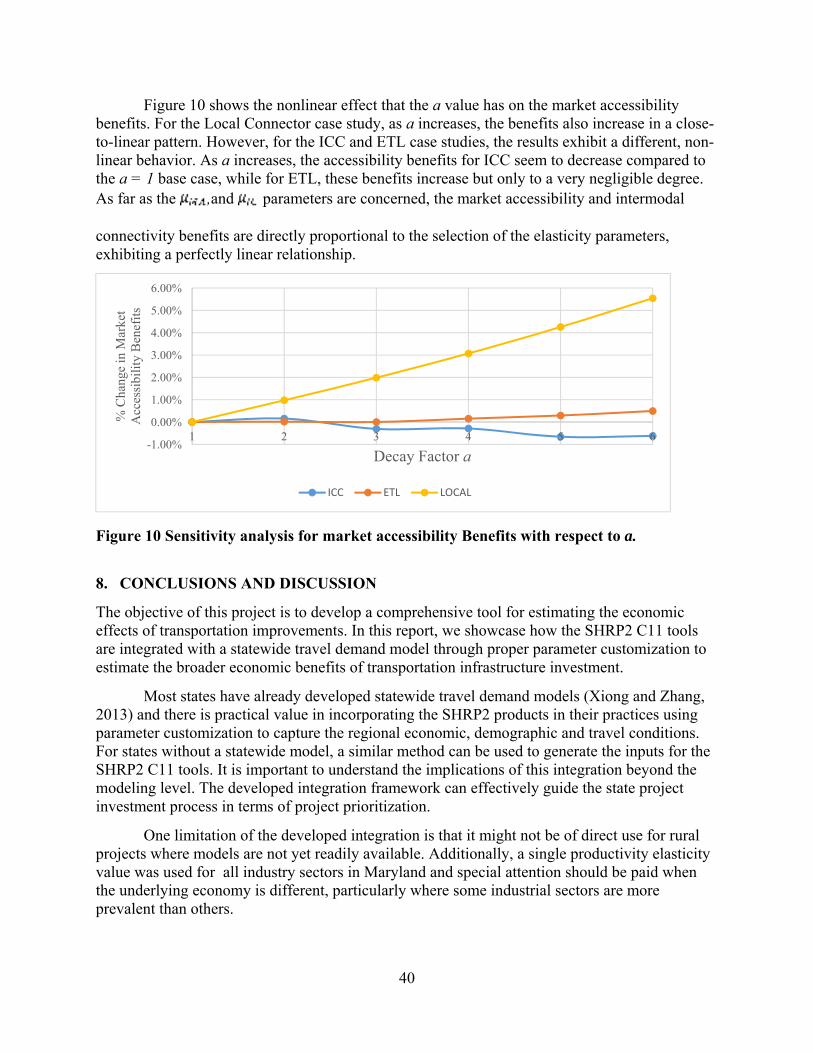
40
Figure 10 shows the nonlinear effect that the a value has on the market accessibility benefits. For the Local Connector case study, as a increases, the benefits also increase in a close-to-linear pattern. However, for the ICC and ETL case studies, the results exhibit a different, non-linear behavior. As a increases, the accessibility benefits for ICC seem to decrease compared to the a = 1 base case, while for ETL, these benefits increase but only to a very negligible degree. As far as the ,and parameters are concerned, the market accessibility and intermodal
connectivity benefits are directly proportional to the selection of the elasticity parameters, exhibiting a perfectly linear relationship.
Figure 10 Sensitivity analysis for market accessibility Benefits with respect to a.
8. CONCLUSIONS AND DISCUSSION
The objective of this project is to develop a comprehensive tool for estimating the economic effects of transportation improvements. In this report, we showcase how the SHRP2 C11 tools are integrated with a statewide travel demand model through proper parameter customization to estimate the broader economic benefits of transportation infrastructure investment.
Most states have already developed statewide travel demand models (Xiong and Zhang, 2013) and there is practical value in incorporating the SHRP2 products in their practices using parameter customization to capture the regional economic, demographic and travel conditions. For states without a statewide model, a similar method can be used to generate the inputs for the SHRP2 C11 tools. It is important to understand the implications of this integration beyond the modeling level. The developed integration framework can effectively guide the state project investment process in terms of project prioritization.
One limitation of the developed integration is that it might not be of direct use for rural projects where models are not yet readily available. Additionally, a single productivity elasticity value was used for all industry sectors in Maryland and special attention should be paid when the underlying economy is different, particularly where some industrial sectors are more prevalent than others.
-1.00%
0.00%
1.00%
2.00%
3.00%
4.00%
5.00%
6.00%
1 2 3 4 5 6
% C
hang
e in
Mar
ket
Acc
essi
bilit
y B
enef
its
Decay Factor a
ICC ETL LOCAL

41
The SHRP2 parameter customization is important in obtaining valid results and obtaining state-specific values is strongly encouraged. It is recommended that states develop their own econometric models to estimate the effect of market accessibility on productivity. The market accessibility benefits are highly sensitive to the α and μ coefficients and their values should be carefully calibrated based on local data. Considering the heterogeneity of a state’s economy, this customization process can be further refined by obtaining region-specific values for the SHRP2 parameters for regions within the state.

42
Figure 11 Streamlined Ratio Approach

43
Figure 12 Comprehensive Framework

44
9. REFERENCES
Agbeli, B.R.D.K. An Empirical Analysis of Three Econometric Frameworks for Evaluating Economic Impacts of Transportation Infrastructure Expenditures Across Countries, Transport Policy, Vol. 35, 2014, pp. 304-310. Agenor, P., Nabli, M. K. and Yousef, T. M., Public Infrastructure and Private Investment in the Middle East and North Africa, Policy Research Working Paper No.3661, World Bank, New York, July 2005. Aschauer, D. A., Is Public Expenditure Productive? Journal of Monetary Economics, 23, 177-200 1989a. Aschauer, D. A., Does Public Capital Crowd Out Private Capital? Journal of Monetary Economics, 24, 1989b, pp.171-188. Assessing Productivity Impacts of Transportation Investments: Final Report and Guidebook, Project NCHRP 02-24, 2014. Bodin, L., E. Miller-Hooks, H. S. Mahmassani, and M. Kim. Economic Impact Study of the Intercounty Connector: Freight and Logistics Impact Assessment. Technical Documentation, Research Report, MTI-SHA-ICC-TD2, Maryland Transportation Initiative, University of Maryland, 2004. Bureau of Labor Statistics, US Department of Labor. Consumer Price Index. June 2015. Cadot, O., Roller, L. and Stephan, A., A Political Economy Model of Infrastructure Allocation: An Empirical Assessment, CEPR Discussion Paper No. 2336, Wissenschaftszentrum, Berlin, December 1999. California Department of Transportation, “California life-cycle, Benefit/Cost Analysis Model” Technical supplement to user’s guide, 1999. Cambridge Systematics, Best Practice Methodology for Calculating Return on Investment for Transportation Programs and Projects NCHRP Report 8-36, Task 62, 2008. Chandra, S., and S. Vadali, S. Evaluating Accessibility Impacts of The Proposed America 2050 High-speed Rail Corridor for The Appalachian Region. Journal of Transport Geography, Vol. 37, 2014, pp. 28-46. Cohen, P.J. The Broader Effects of Transportation Infrastructure: Spatial Econometrics and Productivity Approaches, Transportation Research Part E: Logistics and Transportation Review, Vol. 46, 2010, pp. 317-326. Cohen, J. and Paul, C., Public Infrastructure Investment, Interstate Spatial Spillovers and Manufacturing Costs, The Review of Economics and Statistics, Vol. 86, No. 2, 2004, pp. 551-560.

45
Connecticut Academy of Science and Engineering for the Connecticut Department of Transportation, Analyzing the Economic Impacts of Transportation Projects, 2013. DeCorla-Souza, P., J.T. Hunt, Use of STEAM in evaluating transportation alternatives, 1999. Demetriades, P. and Mamuneas, T., Intertemporal Output and Employment Effects of Public Infrastructure Capital: Evidence from 12 OECD Economies, Economic Journal, Vol. 110, 2000, pp. 687-712. Development of Tools for Assessing Wider Economic Benefits of Transportation Final Report, Strategic Highway Research Program, National Academy of Science, 2013. Dowling Associates, Inc., WSDOT Mobility Project Prioritization Process User’s Guide, 2000. Duffy_Deno, K. T. and R. W. Eberts, Public Infrastructure and Regional Economic Development: A Simultaneous Equations Approach, Journal of Urban Economics, 1991, Vol. 30, pp. 329-343. Finn, M., Is All Government Capital Productive? Federal Reserve Bank of Richmond, Economic Quarterly, Vol. 79, No. 4, Fall 1993, pp. 53-80. Flores de Fretos, R., Garcia-Diez, M. and Prez-Amaral, T., Public Capital Stock and Economic Growth: An Analysis of the Spanish Economy, Applied Economics, Vol. 30, No. 8,1998, pp. 985-994. Graham D., Wider Economic Benefits of Transport Improvements: Link between Agglomeration and Productivity: Stage 1 Report, UK Department for Transport, 2005. He, X., Kastrouni, E., Shayanfar, E., Schonfeld, P. and Zhang, L. Prioritizing Highway Investments: Understanding the Broader Economic Impact of Capacity Expansion and Routine Maintenance. Working Paper. Department of Civil and Environmental Engineering, University of Maryland, College Park, 2014. He, X., Kastrouni, E., and Zhang, L. Impact of Highway Investment on the Economy and Employment across U.S. Industrial Sectors. In Transportation Research Record: Journal of the Transportation Research Board, No. 2452, Transportation Research Board of the National Academies, Washington, D.C., 2015, pp. 1-10. Heyer, C.J., R. McClure. Run-off Reduction BMPs, Real Time Continuous Monitoring Captures Episodic Events, Storm Water Solutions, 2011. IMPLAN Professional, Minnesota IMPLAN Group, INC, Version 2, February 2004.

46
Jiwattanakulpaisarn, P., Noland, R., Graham, D. and Polak, J., Highway Infrastructure Investment and County Employment Growth: A Dynamic Panel Regression Analysis, Journal of Regional Science, Vol. 49, No. 2, 2009, pp. 263-286. Kamps, C., The Dynamic Effects of Public Capital: VAR Evidence for 22 OECD Countries, International Tax and Public Finance, Vol. 12, Issue. 4, 2005, pp. 533-558. Kato, H., Y. Kaneko, and Y. Soyama. Economic Benefits of Urban Rail Projects that Improve Travel-Time Reliability: Evidence from Tokyo, Japan. Transportation Policy, Vol. 35, 2014, pp. 202-210. Kemmerling, A. and Stephan, A., The Contribution of Local Public Infrastructure to Private Productivity and Its Political Economy: Evidence from a Panel of Large German Cities, Public Choice 113, 2002, pp. 403-422. Kernohan, D. and Rognlien, L., Wider Economic Impacts of Transport Investment in New Zealand, NZ Transport Agency Research Report 448,2011. Ligthart, J., Public Capital and Output Growth in Portugal: An Empirical Analysis, European Review of Economics and Finance, Vol. 1, No. 2, 2002, pp. 3-30. Lynch, T., Analyzing the Economic Impact of Transportation Projects Using RIMS ||, IMPLAN and REMI, Office of Research and Special Programs, U.S. Department of Transportation, October 2000. Maryland State Highway Administration. The Maryland Statewide Transportation. Model Documentation. Version 1.0. October 2013. MIG Inc., IMPLAN Pro User’s Guide, 2000. Montana Department of Transportation, Final report “Montana Highway Reconfiguration Study”, 2005. Moreno, R., Lopez-Bazo, E. and Artis, M. , On the Effectiveness of Private and PublicCapital, Applied Economics, Vol. 35, 2003, pp. 727-740. Morrison C. and Schwartz, A., State Infrastructure and Productive Performance, American Economic Review, Vol. 86, No. 5, 1996a, pp. 1095-1111. Morrison C. and Schwartz, A., Public Infrastructure, Private Input Demand and Economic Performance in New England Manufacturing, Journal of Business and Economic Statistics, Vol. 14, No. 1, 1996b, pp. 91-101. Munnell, A. H., Why has Productivity Declined? Productivity and Public Investment, New Egnland Economic Review, Jan./Feb, 1990a., pp. 3-22.

47
Munnell, A. H., How does Public Infrastructure Affect Regional Economic Performance, New England Economic Review, Sep./Oct., 1990b, pp. 11-32. Oregon Department of Transportation, Using HERS-ST for CMS Analysis, 2007. Pereira, A., Public Capital Formation and Private Investment: What Crowds What? Public Finance Review, Vol. 29, No. 1, 2001, pp. 3-25. Pereira, A. and Andraz, J., Public Investment in Transportation Infrastructures and Economic Performance in Portugal, Review of Development Economics, Vol. 9, 2005, pp. 177-196. Pereira, A. and Andraz, J., Public Investment in Transportation Infrastructures and Industry Performance in Portugal, Journal of Economic Development, Vol. 32,2007, pp. 1-20. Pereira, A. and Roca-Sagales, O., Spillover Effects of Public Capital Formation: Evidence from the Spanish Regions, Journal of Urban Economics, Vol. 53,2003, pp. 238-256. Pu, W., S. Mahapatra, M. Tadayon, and D. N. Simpson. Identifying Net Effect of Highway Project in Before-and-After Evaluation. 93rd Annual Meeting of the Transportation Research Board Compendium of Papers, Washington, D.C., 2013. Seitz, H., The Productivity and Supply of Urban Infrastructures, The Annals of Regional Science 29, 1995, pp. 121-141. Shah, A., Dynamics of Public Infrastructure, Industrial Productivity and Profitability, The Review of Economics and Statistics, Vol. 74, No. 1,1992, pp. 28-36. State Highway Administration/Maryland Transportation Authority and Federal Highway Administration. Purpose and Need Statement. http://www.iccproject.com/PDFs/PurposeNeedStatement.pdf. Accessed June 17, 2014. State Smart Transportation Initiative, Economic Effects of Public Investment in Transportation and Directions for the future, 2012. Targa, F., K. J. Clifton, and H. S. Mahmassani. Economic Activity and Transportation Access: An Econometric Analysis of Business Spatial Patterns. In Transportation Research Record: Journal of the Transportation Research Board, No. 1932, Transportation Research Board of the National Academies, Washington, D.C., 2005, pp. 61-71. U.S. Department of Transportation, Federal Highway Administration, “HERS-ST Highway Economic Requirements System- State Version” User’s Guide, 2009. Vijverberg, W., Vijverberg, C. and Gamble, J., Public Capital and Private Productivity, The Review of Economics and Statistics, Vol. 79, No. 2, 1997, pp. 267-278. Weisbord, G., and B. Weisbord. Assessing the Economic Impact of Transportation Projects. Transportation Research Circular, Number 477, 1997.

48
Weisbord, G., T. Lynch, and M. Meyer. Expanding Monetary Values to Broader Performance and Impact Measures: Transportation Applications and Lessons for Other Fields. Evaluation and Program Planning, Vol. 32, 2009, pp. 332-341. Xiong, C., Zhang, L., Deciding Whether and How to Improve Statewide Travel Demand Models Based on Transportation Planning Application Needs. Transportation Planning and Technology, Vol. 36 (3), 2013, pp. 244-266. Zhang, L., Ji, M., Ferrari, N., Comprehensive Highway Corridor Planning with Sustainability Indicators (Final Report), Maryland State Highway Administration, March 2013. Zondag, B., M. De Bok, K. T. Geurs, and E. Molenwijk. Accessibility Modeling and Evaluation: The TIGRIS XL land-use and Transport Interaction Model for The Netherlands. Computers, Environment and Urban Systems, 2014.

49
10. APPENDIX A
Economic Impacts of Transportation Improvements Thank you for participating in our survey.
Here at the National Center for Strategic Transportation Policies, Investment and Decisions in University of Maryland, College Park, we are working closely with the federal and state governments in an effort to quantify the broader economic impacts of transportation infrastructure investment. More particularly, our research group is interested in quantifying direct economic benefits stemming from transportation projects (such as travel time savings, vehicle operating cost savings, reliability performance) but also indirect benefits such as job growth or land-use changes, in the context of a typical Benefit-Cost Analysis.
The ultimate goal of our team is to design a user-friendly tool that federal, state and local agencies will use while performing Benefit-Cost Analysis of project alternatives.
We truly value your participation in our survey as we wish to learn from past experience and build an enhanced, implementation-ready tool. At the end of the survey, please provide us with your contact information, as we wish to share our research findings with you. We would like to thank you in advance for your time.
Research Group: Lei Zhang (Associate Professor), Paul Schonfeld (Professor), Eirini Kastrouni (Graduate Research Assistant), Xiang He (Graduate Research Assistant), Elham Shayanfar (Graduate Research Assistant), Xiushan Jiang (Visiting Scholar)
1. Please provide your affiliation.
2. Does your agency incorporate Benefit-Cost Analysis or an Economic Impact Analysis Component in its decision-making process?
Yes
No 3. Does your agency use any particular software tool for Benefit-Cost or Economic Impact Analysis?
Yes
No
4. If so, which tool have you been using [select all that apply]?
BCA.Net
Cal-B/C
HERS-ST
MicroBENCOST
STEAM
SHRP-2
StratBENCOST
HEAT
Other [Please provide tool name]

50
Specify other tools
5. How long have you been using the tool(s)?
6.What is your experience?
Satisfied
Somewhat Satisfied
Neutral
Somewhat Dissatisfied
Dissatisfied
7.Please identify any particular issues with the tool you are using [select all that apply]:
Issues with default data
Concerns with methodology
Issues with User Interface
Issues with User Guide
Issues with the list of performance measures generated by the software
No issues/concerns; I am satisfied with the tool.
Other issues Please explain (optional):
8.Does your agency incorporate the tool’s output in the decision-making process?
Yes
No

51
If so, can you briefly explain how?
Please provide any additional coments
9.Please provide your contact information in the event we need to follow-up with you:
Name
E-mail address (*)
Phone number (*)
SUBMIT

52
11. APPENDIX B
Life-Cycle Project Evaluation
In project evaluation, one common approach for comparing projects with unequal economic lives is to estimate the equivalent uniform annual cash flow generated by each project over its lifespan. This calculation represents the net present value of an investment as a series of equal cash flows distributed uniformly over the investment’s life. For this purpose, the Net Annual Benefits ( ), also known as Equivalent Annual Flow ( ), are computed as:
1 ∗1 1
(1)
where denotes initial benefits (in this study, = 0); is the capital recovery factor; i represents the yearly interest rate; n is the economic life of facilities in years, and , , indicate annual benefits, initial costs (including mainly land and construction) and annual costs, respectively. This estimation is especially important in this study since it provides the adjusted annual benefits with regards to both initial and operational costs, and allows for better comparisons among projects. For this calculation, the authors assumed baseline values of 60 years for the economic life of projects, 5 percent for the interest rate, and 3 percent for the operation and maintenance costs as a fraction of each project’s initial cost. The effects of these parameters are explored through sensitivity analyses around those baseline values. The above formulation can be easily modified if there are some final benefits (e.g. salvage value), final costs (e.g. demolition, clean-up), or some intermediate costs and benefits (e.g. expansion or rehabilitation).